Preprint: Final version has appeared in: Science 338:60-65 (2012)

Theory and Simulation in Neuroscience Wulfram Gerstner

1,*, Henning Sprekeler

2,3,4, and Gustavo Deco

5,6 1

School of Computer and Communication Sciences and Brain Mind Institute, School of Life

Sciences, Ecole Polytechnique Fédérale de Lausanne, 1015 Lausanne EPFL, Switzerland 2

Technische Universität Berlin, Germany 3

Humboldt-Universität zu Berlin, Germany 4

Bernstein Center for Computational Neuroscience Berlin, Germany 5

Center for Brain and Cognition, Dept. of Information and Communications Technologies, Universitat Pompeu Fabra, Barcelona, Spain 6

ICREA (Institució Catalana de Recerca i Estudis Avançats), Roc Boronat 138, Barcelona, Spain *

corresponding author, wulfram.gerstner@epfl.ch Abstract: Modeling work in neuroscience can be classified using two different criteria. The first one is the complexity of the model ranging from simplified conceptual models that are amenable to mathematical analysis to detailed models that require simulations in order to understand their properties. The second criterion is that of direction of workflow, which can be from microscopic to macroscopic scales (bottom-up) or from behavioral target functions to properties of components (top- down). We review the interaction of theory and simulation using examples of top-down and bottom-up studies and point to some current developments in the fields of computational and theoretical neuroscience.

Mathematical and computational approaches in neuroscience have a long tradition that can be followed back to early mathematical theories of perception [1, 2] and of current integration by a neuronal cell membrane [3]. Hodgkin and Huxley combined their experiments with a mathematical description, which they used for simulations on one of the early computers [4]. Hebb’s ideas on assembly formation [5] have, already in 1956, inspired simulations on the largest computers available at that time [6]. Since the 1980ies the field of theoretical and computational neuroscience has grown enormously [7]. Modern neuroscience methods requiring extensive training have led to a specialization of researchers so that neuroscience today is fragmented into labs working on genes and molecules; on single-cell electrophysiology; on multi-neuron recordings; on cognitive neuroscience and psychophysics, to name just a few. One of the central tasks of computational neuroscience is to bridge these different levels of description by simulation and mathematical theory. The bridge can be built in two different directions. Bottom-up models integrate what is known on a lower level (e.g., properties of ion channels) to explain phenomena observed on a higher level (e.g., generation of action potentials [4, 8–10]). Top-down models, on the other hand, start with known cognitive functions of the brain (e.g., working memory), and deduce from these how components (e.g., neurons or groups of neurons) should behave to achieve these functions. Influential examples of the top-down approach are theories of associative memories [11, 12], reinforcement learning [13, 14], and sparse coding [15, 16]. Bottom-up and top-down models can either be studied by mathematical theory (theoretical neuroscience) or by computer simulations (computational neuroscience). Theory has the advantage of providing a complete picture of the model behavior for all possible parameter settings, but analytical solutions are restricted to relatively simple models. The aim of theory is therefore to purify biological ideas to the bare minimum, so as to arrive at a ’toy model’, which crystallizes a concept in a set of mathematical equations that can be fully understood. Simulations, in contrast, can be applied to all models, simplified as well as complex ones, but they can only sample the model behavior for a limited set of parameters. If the relevant parameters were known, the whole or a major fraction of the brain could be simulated using known biophysical components, a prospect that has inspired recent large-scale simulation projects [17–21]. How can theory and simulation interact to contribute to our understanding of brain function? In this article, we illustrate the interaction with four case studies and outline future avenues for synergies between theory and simulation. Even though it forms an important subfield of computational neuroscience, the analysis of neuronal data [22–24] is not included in this review.

From detailed to abstract models of neural activity: Bottom-up theory

The brain contains billions of neurons, which communicate by short electrical pulses, called action potentials or spikes. Hodgkin and Huxley’s description of neuronal action potentials [4] provides today a basis for standard simulator software [25, 26] and, more generally a widely used framework for biophysical neuron models. In these models, each patch of cell membrane is described by its composition of ion channels, with specific time constants and gating dynamics that control the momentary state (open or closed) of a channel (Fig. 1C).

By a series of mathematical steps and approximations, theory has sketched a systematic bottom-up path from such biophysical models of single neurons to macroscopic models of neural activity. In a first step, biophysical models of spike generation are reduced to integrate-and-fire models [27–32] where spikes occur whenever the membrane potential reaches the threshold (Fig. 1B). In the next abstraction step, the population activity A(t) – defined as the total number of spikes emitted by a population of interconnected neurons in a short time window – is predicted from the properties of individual neurons [33–35] using mean-field methods known from physics: because each neuron receives input from many others, it is sensitive only to their average activity (’mean field’) but not to the activity patterns of individual neurons. Instead of the spike-based interaction between thousands of neurons, network activity can therefore be described macroscopically as an interaction between different populations [36, 33, 35]. Such macroscopic descriptions are called population models, neural mass models or, in the continuum limit, neural field models (Fig. 1A) and help researchers to gain an intuitive and more analytical understanding of the principal activity patterns in large networks. While the transition from microscopic to macroscopic scales relies on purely mathematical arguments, simulations are important to add biological realism such as heterogeneity of neurons and connectivity, adaptation on slower time scales, variability of input and receptive fields, which are difficult to treat

mathematically; but the theoretical concepts and the essence of the phenomena are often robust with respect to these aspects.

Decision Making: Theory combines top-down and bottom-up

Many times a day we are confronted with a decision between two alternatives (A or B), like ‘Should I turn left or right?’. Psychometric measures of performance and reaction times for two-alternative forced-choice decision-making paradigms can be fitted by a phenomenological drift-diffusion model [37]. This model consists of a diffusion equation describing a random variable that accumulates noisy sensory evidence until it reaches one of two boundaries, corresponding to a specific choice (Fig. 2A). Despite its success in explaining reaction time distributions, the drift-diffusion model suffers from a crucial disadvantage, namely the difficulty in assigning a biological meaning to the model parameters. Recently, neurophysiological experiments have begun to reveal neuronal correlates of decision making, in tasks involving visual patterns of moving random dots [41,42], vibrotactile [43] or auditory frequency comparison [44]. Computational neuroscience offers a framework to bridge the conceptual gap between the cellular and the behavioral level. Explicit simulations of microscopic models based on local networks with large numbers of spiking neurons can reproduce and explain both the neurophysiological and behavioral data [45, 39]. These models describe the interactions between two groups of neurons coupled through mutually inhibitory connections (Fig. 2C). Suitable parameters are inferred by studying the dynamical regimes of the system and choosing parameters consistent with the experimental observations of decision behavior. Thus, the pure bottom-up path is complemented by the top-down insights of target functions that the network needs to achieve.

Interestingly, theory has provided a way to identify the connection between the simulation-based biophysical level and the phenomenological drift-diffusion models that were used to quantify behavioral data in the past. This analysis first involves reducing the system of millions of differential equations to only two equations, by the mean-field techniques [33] discussed in the previous paragraph (cf. Fig. 1A). In this reduced system, different dynamical regimes can be studied by means of a bifurcation diagram (Fig. 2B), leading to a picture in which the dynamics of decision making can be visualized as a ball rolling down into one of the minima of a multi-well energy landscape. Close to the bifurcation point (DD), finally, the dynamics can be further reduced to a non-linear one-dimensional drift-diffusion model [46] (Fig. 2A).

Hebbian assemblies and associative memories: Top-down concepts

The name of Hebb is attached to two different ideas that are intimately linked [5]: the Hebbian cell assembly and the Hebbian learning rule. The former states that mental concepts are represented by the joint activation of groups of cells (assemblies). The latter postulates that these assemblies are formed by strengthening the connections between neurons that are ’repeatedly and persistently active together’. These strong connections enable the network to perform an associative retrieval of memories (Fig. 3A): if a neuron that is part of the assembly does not receive an external stimulus sufficient to trigger its firing, it can nevertheless be activated by lateral excitatory input from active partners in the assembly, such that eventually the stored activity pattern is completed and the full assembly – and thus the memory – is retrieved. While Hebb wrote down his ideas in words, it soon inspired mathematical models of learning rules and large-scale simulation studies [6]. Whereas the simulations pointed to limitations of Hebb’s original ideas in practical applications, mathematical studies [11, 48, 49] cleared first paths through the jungle of possible model configurations toward a working model of memory retrieval. In analogy to models of magnetic systems and spin glasses in statistical physics, the picture of memory retrieval as movement toward a minimum in an energy landscape emerged (Fig. 3B), first in networks of binary units [50, 12], later also for rate models [51, 52]. In these frameworks, important questions could be answered, such as that of memory capacity. Because each neuron can participate in many different assemblies, memory capacity is difficult to estimate by pure verbal reasoning. Theory shows that the number of different random patterns that can be stored scales linearly with the number of neurons [53]: a network with 10,000 neurons can store about 1000 patterns, but if we double the number of neurons, we can store twice as many. It took many steps from these abstract concepts to arrive at biologically plausible models of memory. Whereas the energy landscape analogy is restricted to a limited class of abstract models, the concept of memory retrieval as movement towards an attractor state (Fig. 3C) turned out to be robust with respect to model details. The top-down path (Fig. 3C-E) of model development includes the transition from high-activity states to low-activity states [54]; from networks with complete and reciprocal connectivity to ones with sparse and asymmetric connections [55]; tuning of inhibition in sparsely active networks [56]; transition from rate neurons to spiking neurons [57, 34, 58]; addition of a spontaneous state at low firing rates [59, 60]; homeostatic control of threshold or plasticity [61, 47]; and further steps still to be taken, so as to solve the issue of online-learning in associative memory networks [62]. The above historical sketch shows the flow of

ideas from top to bottom, by adding biological realism and details to well-understood abstract concepts. As research moves along this path, numerical simulations gain in importance, but theory remains the guiding principle. Given the technical challenges of detecting distributed but jointly active neuronal assemblies in the brain, it is not surprising that experimental evidence for associative memories as attractor states remains scarce and indirect: neither invariant sensory representations as observed in individual high-level neurons [63] nor persistent activity during working memory tasks [64, 65] are sufficient to prove attractor dynamics, and the interpretation of multi-unit recordings during remapping in hippocampus as signature of attractors [66] has been questioned [67], so that novel experimental approaches that enable large-scale recordings of complete neural ensembles [68–70] will be necessary.

Reward-based learning: From behavior to synapse

Hebbian assemblies play a role in models of decision making (e.g., two populations representing choices A or B), but the assemblies are fixed and do not change. As such, these models describe static stimulus-response mappings that do not take into account that we can alter our decision strategies that we can learn from experience. Theories of behavioral learning are an example for a top-down approach that has led from psychology to models of synaptic plasticity, which go beyond a simple Hebbian learning rule. Models of behavioral learning date back to early experimental psychology. Thorndike’s ”law of effect” [71] already stated that animals use behavioral alternatives more often when they were rewarded in the past. The mathematical theory of Rescorla and Wagner [13] extended this idea and suggested that it is not reward per se that drives learning, but the discrepancy between actual and expected outcome, an insight that is also essential in models of temporal difference learning [72]. In the 1980s, this line of research on trial-and-error learning in animal psychology and artificial intelligence joined the parallel, mainly engineering-driven line of control theory [73] to form the large research field of reinforcement learning [74]. Although reinforcement learning often makes use of neural architectures [75, 76], its main focus is algorithmic. The renewed interest of computational and theoretical neuroscience in reward-based learning was triggered in the 1990’s by two physiological findings. First, Schultz and colleagues discovered that dopamine neurons in the midbrain respond to unexpected rewards [77] with activity patterns that resemble the reward prediction error of temporal difference learning [14]. Moreover, it was shown that synaptic plasticity, long hypothesized to form the neural basis of learning [78], is under dopaminergic control [79–81] and thus modulated by reward prediction errors. These findings have led to the idea that the traditional Hebbian view of synaptic plasticity driven by pre- and postsynaptic activity has to be augmented by reward prediction error as a third factor [80]. The current tasks of computational neuroscience are to compare the learning rules suggested by the top-down approach with experimental data, and generalize existing concepts in order to evaluate if and under which conditions 3-factor learning rules [82–84] of reward-modulated Hebbian synaptic plasticity can be useful at the macroscopic level of networks [85, 86] and behavior [87, 88]. Reinforcement learning is a textbook example for a synergistic interaction of theory and simulation. Most algorithms are based on mathematical theory, but without an actual implementation and simulation, it is difficult to predict how they perform under realistic conditions. The undesired increase in learning time with problem complexity observed in simulations of most algorithms poses challenges for the future. The solution could lie in efficient representations of actions [89] as well as environmental and bodily states [90], possibly adapted through Hebbian learning; place cells could serve here as an example [91, 92]. Large-scale simulations will be key to evaluating whether neuronal representations across different brain areas are apt to turn complex reward-based learning tasks into simple ones - or whether we need a paradigm shift in reward-based learning.

Large-Scale Simulation needs Theory

With the growth of computer power, the notion of large-scale simulation continues to change. While in the 1950s, networks of 512 binary neurons were explored on the supercomputers of that time [6], network size and biological realism increased in the 1980s to 9900 detailed model neurons [93]. Current simulations of

networks go up to 109[94] or 10

11 [95] integrate-and-fire neurons or 10

6 multi-compartment integrate-and-fire

models with synaptic plasticity [96]. The structure of neural networks, which is intrinsically distributed and parallel, lends itself to implementations on highly parallel computing devices (e.g., [97, 98]), and has triggered specialized ’neuromorphic’ design of silicon circuits [99, 100]. Future implementations of large networks of integrate-and-fire neurons with synaptic plasticity on specialized parallel hardware [101–104] should run much faster than biological real time, opening the path toward rapid exploration of learning paradigms. Current large-scale implementations on general-purpose or specialized computing devices are feasibility studies suggesting that the simulation of

neural networks of the size of real brains is possible. But before such simulations become a tool of brain science, major challenges need to be addressed - and this is where theory comes back into play. First, theory supports simulations across multiple spatial scales. Even on the biggest computers it is impossible to simulate the whole brain at a molecular resolution, but, for, e.g., a study of the interaction of a drug with a synapse, the synapse could be simulated at the molecular level; the neuron on which the synapse sits at the level of biophysical model neurons; the brain area in which the circuit is embedded at the level of integrate-and-fire models; and the remaining brain areas are summarized in population equations that describe their mean activity. Theory provides the methods to systematically bridge the scales while ensuring the self-consistency of the model. Second, theories guide simulations of learning. Because learning (at the behavioral level) and long-term plasticity of synapses (at the cellular level) evolve on the time scale of hours, experimental progress is slow and data to constrain synaptic plasticity rules are scarce. Even before a candidate plasticity rule is implemented in a simulation, theories allow to predict, in some cases, that a given rule cannot work for the task at hand, while another one should work, but might be slow, and yet another one should work perfectly, if combined with some finely tuned homeostatic process, etc. Third, regularization theories provide a framework for optimization of parameters. Already at the level of a single neuron the number of parameters is huge considering the fact that there are about 200 different types of ion channels [105] and that the density of ion channels varies along the dendrite. Moreover, in a network of billions of neurons, each with thousands of connections, the number of parameters to specify the connectivity is daunting. How then, can experimental findings ever sufficiently constrain such detailed models? A solution to this problem could be provided by regularization theory, which penalizes parameter settings that deviate from what is considered plausible. The challenge in the application of regularization to biologically detailed neural networks consists in designing appropriate regularization terms that summarize plausible prior assumptions in a transparent fashion. For example, ion channel distributions along a dendrite can be regularized by imposing plausible density profiles [10, 106], and penalizing the use of more than a few channels for any neuron [107]. Connectivity can be regularized by penalizing deviations from simple ‘connectivity rules’ [108, 109]. Fourth, theory drives understanding. It is extremely difficult to control a complex simulation if we do not have an intuition of the basic mechanisms at work. Mathematical abstraction forces us to express intuitions rigorously, to turn ideas into toy models. These not only make qualitative predictions of how a complex simulation should behave under changes of parameters, but also provide the understanding necessary to communicate ideas to others.

Theory Needs Simulations

While theoretical concepts exist for some aspects of brain function, theoretical neuroscience is not finished and big challenges lie ahead of it regarding, e.g., neurally plausible models of verbal and mathematical reasoning or representations of language and music. Will existing and future concepts developed in mathematical toy models be transferable to systems of the size of a brain with realistic input and output? The authors believe so, but currently extensions to large systems cannot be tested. In our opinion, mathematical toy models will continue to play a major role in guiding the way we think about neuroscience. However, in order to avoid that the biggest problems addressed in computational neuroscience are limited to the size of one PhD project, initiatives for shared modular and reusable code and standardized simulator interfaces [110–113] are important. More generally, the community of theoretical and computational neuroscience would profit from a simulation environment where the ideas developed in the toy models could be tested on a larger scale, in a biologically plausible setting, and where the ideas arising in different communities and labs are finally connected to the bigger whole.

Acknowledgements

Research was supported by the European Research Council (no. 268 689, W.G. and 295129, G.D.), the European Community’s Seventh Framework Program (grant agreements no. 243914, Brain-I-Nets, W.G. and H.S.; and no. 269921, BrainScaleS, W.G. and G.D.), the Swiss National Science Foundation (grants no. 200020 132871) and the Spanish Ministerio de Economia y Competitividad (grants no. CDS-2007-00012 and SAF2010-16085). We thank T. Vogels for helpful discussions.

References and Notes [1] H. Helmholtz. Die Lehre von den Tonempfindungen als physiologische Grundlage für die Theorie der Musik, 6th Edition. Vieweg, 1913. 1st published in 1862.

[2] Ernst Mach. Die Analyse der Empfindungen (chapter X). Gustav Fischer, Jena, 5th edition, 1906. http://www.uni-leipzig.de/psycho/wundt/opera/mach/empfndng/AlysEmIn.htm. [3] L. Lapicque. Recherches quantitatives sur l’excitation electrique des nerfs traitée comme une polarization. J. Physiol. Pathol. Gen., 9:620–635, 1907. [4] A.L. Hodgkin and A.F. Huxley. A quantitative description of membrane current and its application to conduction and excitation in nerve. J Physiol, 117(4):500–544, 1952. [5] D. O. Hebb. The Organization of Behavior. Wiley, New York, 1949. [6] N. Rochester, J. Holland, L. Haibt, and W. Duda. Tests on a cell assembly theory of the action of the brain, using a large digital computer. IRE Trans. Inf. Theory, 2:80–93, 1956. [7] L.F. Abbott. Theoretical neuroscience rising. Neuron, 60:489–494, 2008. [8] W. Rall. Cable theory for dendritic neurons. In C. Koch and I. Segev, editors, Methods in Neuronal Modeling, pages 9–62, Cambridge, 1989. MIT Press. [9] Z. F. Mainen, J. Joerges, J. R. Huguenard, and T. J. Sejnowski. A model of spike initiation in neocortical pyramidal neurons. Neuron, 15(6):1427–1439, 1995.

rmann, H. Markram, and I. Segev. Models of neocortical layer 5b pyramidal cells capturing a

wide range of dendritic and perisomatic active properties. PLoS Comput. Biol., 7:e1002107, 2011. [11] D. J. Willshaw, O. P. Buneman, and H. C. Longuet-Higgins. Non-holographic associative memory. Nature, 222:960–962, 1969. [12] J. J. Hopfield. Neural networks and physical systems with emergent collective computational abilities. Proc. Natl. Acad. Sci. USA, 79:2554–2558, 1982. [13] R. A. Rescorla and A. R. Wagner. A theory of Pavlovian conditioning: variations in the effectiveness of reinforcement and nonreinforcement. In A. H. Black and W.F. Prokasy, editors, Classical Conditioning II: current research and theory, pages 64–99. Appleton Century Crofts, New York, 1972. [14] W. Schultz, P. Dayan, and R. R. Montague. A neural substrate for prediction and reward. Science, 275:1593–1599, 1997. [15] H. B. Barlow. Possible principles underlying the transformation of sensory messages. In W. A. Rosenbluth, editor, Sensory Communication, pages 217–234. MIT Press, 1961. [16] B. A. Olshausen and D. J. Field. Sparse coding of sensory inputs. Current Opinion in Neurobiology, 14(4):481–487, 2004. [17] DARPA SyNAPSE Program. http://www.artificialbrains.com/darpa-synapse-program. [18] BrainCorporation. http://braincorporation.com. [19] S. Lang, V. J. Dercksen, B. Sakmann, and M. Oberländer. Simulation of signal flow in 3D reconstructions of an anatomically realistic neural network in rat vibrissal cortex. Neural Networks, 24:998–1011, 2011. [20] BrainScales. https://brainscales.kip.uni-heidelberg.de/. [21] H. Markram. The Blue Brain Project. Nat Rev Neurosci, 7(2):153–160, 2006. [22] F. Rieke, D. Warland, R. de Ruyter van Steveninck, and W. Bialek. Spikes - Exploring the neural code. MIT Press, Cambridge, MA, 1996.

[23] J.W. Pillow, J. Shlens, L. Paninski, A. Sher, A. M. Litke, E. J. Chichilnisky, and E.P. Simoncelli. Spatio-temporal correlations and visual signalling in a complete neuronal population. Nature, 454:995–999, 2008. [24] R. Q. Quiroga and S. Panzeri. Extracting information from neuronal populations: information theory and decoding approaches. Nature Reviews Neuroscience, 10:173–185, 2009. [25] M. L. Hines and T. Carnevale. The NEURON simulation environment. Neural Computation, 9:1179–1209, 1997. [26] J. M. Bower and D. Beeman. The book of Genesis. Springer, New York, 1995. [27] A. V. M. Herz, T. Gollisch, C. K. Machens, and Dieter Jaeger. Modeling single-neuron dynamics and computations: a balance of detail and abstraction. Science, 314(5796):80–85, 2006. [28] W. M. Kistler, W. Gerstner, and J. Leo van Hemmen. Reduction of Hodgkin-Huxley equations to a single-variable threshold model. Neural Comput., 9:1015–1045, 1997.

[29] G. B. Ermentrout. Type I membranes, phase resetting curves, and synchrony. Neural Computation, 8(5):979–1001, 1996. [30] N. Fourcaud-Trocme, D. Hansel, C. van Vreeswijk, and N. Brunel. How spike generation mechanisms determine the neuronal response to fluctuating input. J. Neuroscience, 23:11628–11640, 2003. [31] R. Jolivet, T. J. Lewis, and W. Gerstner. Generalized integrate-and-fire models of neuronal activity approximate spike trains of a detailed model to a high degree of accuracy. J. Neurophysiol., 92:959–976, 2004. [32] R. Brette and W. Gerstner. Adaptive exponential integrate-and-fire model as an effective description of neuronal activity. J. Neurophysiol., 94:3637 – 3642, 2005. [33] N. Brunel. Dynamics of sparsely connected networks of excitatory and inhibitory neurons. Computational Neuroscience, 8:183–208, 2000. [34] S. Fusi and M. Mattia. Collective behavior of networks with linear (VLSI) integrate and fire neurons. Neural Computation, 11:633–652, 1999. [35] W. Gerstner. Population dynamics of spiking neurons: fast transients, asynchronous states and locking. Neural Computation, 12:43–89, 2000. [36] H. R. Wilson and J. D. Cowan. Excitatory and inhibitory interactions in localized populations of model neurons. Biophys. J., 12:1–24, 1972. [37] R. Ratcliff and J. N. Rouder. Modeling response times for two-choice decisions. Psychol. Sci., 9:347–356, 1998. [38] X. J. Wang. Decision making in recurrent neuronal circuits. Neuron, 60:215–234, 2008. [39] G. Deco, E. T. Rolls, and R. Romo. Stochastic dynamics as a principle of brain function. Progr. Neurobiol., 88:1–16, 2009. [40] K. F. Wong and X. J. Wang. A recurrent network mechanism of time integration in perceptual decisions. J. Neurosci., 26:1314–1328, 2006. [41] J. I. Gold and M. N. Shadlen. Neural computations that underlie decisions about sensory stimuli. Trends Cog. Sci., 5:10–16, 2001. [42] J. I. Gold and M. N. Shadlen. The neural basis of decision making. Ann. Rev. Neurosci., 30:535–574, 2007. [43] R. Romo and E. Salinas. Flutter discrimination: neural codes, perception, memory and decision making. Nature Rev. Neurosci., 4:203–218, 2003. [44] L. Lemus, A. Hernandez, and R. Romo. Neural encoding of auditory discrimination in ventral premotor cortex. Proc. Natl. Acad. Sci (USA), 106:14640–14645, 2009. [45] X.-J. Wang. Probabilistic decision making by slow reverberation in cortical circuits. Neuron, 36:955–968, 2002. [46] A. Roxin and A. Ledberg. Neurobiological models of two-choice decision making can be reduced to a one-dimensional nonlinear diffusion equation. PLOS Comput. Biol., 4:e1000046, 2008.

[47] T. P. Vogels, H. Sprekeler, F. Zenke, C. Clopath, and W. Gerstner. Inhibitory plasticity balances excitation and inhibition in sensory pathways and memory networks. Science, 334:1569–1731, 2011. [48] J. A. Anderson. A simple neural network generating an interactive memory. Math. Biosc., 14:197–220, 1972. [49] T. Kohonen. Correlation matrix memories. IEEE Trans. on computers, 100:353–359, 1972. [50] W. A. Little. The existence of persistent states in the brain. Math. Biosc., 19:101–120, 1974. [51] M. A. Cohen and S. Grossberg. Absolute stability of global pattern formation and parallel memory storage by competitive neural networks. IEEE Trans. on systems, man, and cybernetics, 13:815–823, 1983. [52] J. J. Hopfield. Neurons with graded response have computational properties like those of two–state neurons. Proc. Natl. Acad. Sci. USA, 81:3088–3092, 1984. [53] D. J. Amit, H. Gutfreund, and H. Sompolinsky. Storing infinite number of patterns in a spin-glass model of neural networks. Phys. Rev. Lett., 55:1530–1533, 1985. [54] D. J. Amit, H. Gutfreund, and H. Sompolinsky. Information storage in neural networks with low levels of activity. Phys. Rev. A, 35:2293–2303, 1987. [55] B. Derrida, E. Gardner, and A. Zippelius. An exactly solvable asymmetric neural network model. Europhysics Letters, 4:167–173, 1987. [56] D. Golomb, N. Rubin, and H. Sompolinsky. Willshaw model: associative memory with sparse coding and low firing rates. Phys. Rev. A, 41:1843–1854, 1990.

[57] W. Gerstner and J. L. van Hemmen. Associative memory in a network of ‘spiking’ neurons. Network, 3:139–164, 1992. [58] D. J. Amit and M. V. Tsodyks. Quantitative study of attractor neural networks retrieving at low spike rates. I: Substrate — spikes, rates, and neuronal gain. Network, 2:259–273, 1991. [59] D. J. Amit and N. Brunel. Dynamics of a recurrent network of spiking neurons before and following learning. Network, 8:373–404, 1997. [60] N. Brunel and V. Hakim. Fast global oscillations in networks of integrate-and-fire neurons with low firing rates. Neural Computation, 11:1621–1671, 1999. [61] J. Triesch. Synergies between intrinsic and synaptic plasticity mechanisms. Neural Computation, 19:885 –909, 2007. [62] S. Fusi. Hebbian spike-driven synaptic plasticity for learning patterns of mean firing rates. Biol. Cybern., 87:459– 470, 2002. [63] R. Q. Quiroga, L. Reddy, G. Kreiman, C. Koch, and I. Fried. Invariant visual representation by single neurons in the human brain. Nature, 435:1102–1107, 2005. [64] J.M. Fuster and G.E. Alexander. Neuron activity related to short-term memory. Science, 173:652–654, 1971. [65] E. K. Miller and J. D. Cohen. An integrative theory of prefrontal cortex function. Ann. Rev. Neurosci., 24:167–202, 2001. [66] T. J. Wills, C. Lever, F. Cacucci, N. Burgess, and J. O’Keefe. Attractor dynamics in the hippocampal representation of the local environment. Science, 308:873–876, 2005. [67] K. J. Jeffery. Place cells, grid cells, attractors, and remapping. Neural Plasticity, 2011:182602, 2011. [68] D. S. Greenberg, A. R. Houweling, and J. N. D. Kerr. Population imaging of ongoing neuronal activity in the visual cortex of awake rats. Nature Neuroscience, 11:749–751, 2008. [69] B. F. Grewe and F. Helmchen. Optical probing of neuronal ensemble activity. Current Opinion in Neurobiology, 19:520–529, 2009. [70] C. Koch and R.C. Reid. Neuroscience: Observatories of the mind. Nature, 483:397–398, 2012.

[71] E. L. Thorndike. Animal Intelligence. Hafner, Darien, CT, 1911. [72] R. Sutton. Learning to predict by the method of temporal differences. Machine learning, 3:9–44, 1998. [73] D. P. Bertsekas. Dynamic programming and stochastic control, volume 125. Academic Pr, 1976. [74] R. Sutton and A. Barto. Reinforcement learning. MIT Press, Cambridge, 1998. [75] A. G. Barto, R. S. Sutton, and C. W. Anderson. Neuronlike adaptive elements that can solve difficult learning and control problems. IEEE transactions on systems, man, and cybernetics, 13:835–846, 1983. [76] R. Sutton and A. Barto. Time-derivative models of Pavlovian reinforcement. In M. Gabriel and J. Moore, editors, Learning and Computational Neuroscience: Foundations of Adaptive Networks, pages 497–537. MIT Press, Cambridge, 1990. [77] P. Apicella, T. Ljungberg, E. Scarnati, and W. Schultz. Responses to reward in monkey dorsal and ventral striatum. Exp. Brain Research, 85:491–500, 1991. [78] S. J. Martin, P. D. Grimwood, and R. G. M. Morris. Synaptic plasticity and memory: an evaluation of the hypothesis. Ann. Rev. Neurosci., 23:649–711, 2000. [79] P. Calabresi, R. Maj, N. B. Mercuri, and G. Bernandi. Coactivation of D1 and D2 dopamine receptors is required for long-term synaptic depression in the striatum. Neurosci. Lett., 142:95–99, 1992. [80] J. N. J. Reynolds and J. R. Wickens. Dopamine-dependent plasticity of corticostriatal synapses. Neural Networks, 15:507–521, 2002. [81] V. Pawlak, J. R. Wickens, A. Kirkwood, and J. N. D. Kerr. Timing is not everything: neuromodulation opens the STDP gate. Front. Synaptic Neurosci., 2:146, 2010. [82] X. Xie and S. Seung. Learning in neural networks by reinforcement of irregular spiking. Phys. Rev. E, 69:41909, 2004. [83] E. M. Izhikevich. Solving the distal reward problem through linkage of STDP and dopamine signaling. Cerebral Cortex, 17:2443–2452, 2007. [84] R. V. Florian. Reinforcement learning through modulation of spike-timing-dependent synaptic plasticity. Neural Computation, 19:1468–1502, 2007. [85] N. Frémaux, H. Sprekeler, and W. Gerstner. Functional requirements for reward-modulated spike-timing-dependent plasticity. J. Neurosci., 40:13326–13337, 2010. [86] R. Legenstein, S. M. Chase, A. B. Schwartz, and W. Maass. A reward-modulated Hebbian learning rule can explain experimentally observed network reorganization in a brain control task. J. Neurosci., 30:8400–8410, 2010. [87] Y. Loewenstein and H.S. Seung. Operant matching is a generic outcome of synaptic plasticity based on the covariance between reward and neural activity. Proc. Natl. Acad. Sci. USA, 103:15224–15229, 2006. [88] M.H. Herzog, K.C. Aberg, N. Frémaux, W. Gerstner, and H. Sprekeler. Perceptual learning, roving, and the unsupervised bias. Vision Research, 61:95–99, 2012. [89] A.G. Barto and S. Mahadevan. Recent advances in hierarchical reinforcement learning. Discrete Event Dynamic Systems, 13(4):341–379, 2003. [90] S. Mahadevan and M. Maggioni. Proto-value functions: A Laplacian framework for learning representation and control in Markov decision processes. Journal of Machine Learning Research, 8(2169-2231):16, 2007. [91] D. Foster, R. Morris, and P. Dayan. Models of hippocampally dependent navigation using the temporal difference learning rule. Hippocampus, 10:1–16, 2000. [92] D. Sheynikhovich, R. Chavarriaga, T. Strosslin, A. Arleo, and W. Gerstner. Is there a geometric module for spatial orientation? Insights from a rodent navigation model. Psychological Review, 116:540–566, 2009. [93] R. D. Traub, R. Miles, and R. K. S. Wong. Large scale simulations of the hippocampus. IEEE engineering in medicine and biology, 7(31-38), 1988.

[94] R. Ananthanarayanan, S.K. Esser, H.D Simon, and D. S. Modha. The cat is out of the bag: cortical simulations with

109

neurons, 1013

synapses. Proc. Conf. high performance computing networking, storage and analysis, 2009. [95] E.Izhikevich.Simulation of large scale brain models. http://www.izhikevich.org/human−brain−simulation/, 2005 [96] E. M. Izhikevich and G. M. Edelman. Large-scale model of mammalian thalamocortical systems. Proc. Nat. Acad. Sci. (USA), 105(9):3593–3598, 2008. [97] K. Obermayer, H. Ritter, and K. Schulten. Large-scale simulations of self-organizing neural networks on parallel computers: application to biological modeling. Parallel computing, 14:381–404, 1990. [98] E. Niebur and D. Brettle. Efficient simulation of biological neural networks on massively parallel supercomputers with hypercube architecture. In J. Cowan, G. Tesauro, and J. Alspector, editors, Advances Neur. Inf. Proc. Systems, volume 6, pages 904–910. Morgan Kaufmann, San Mateo, 1994. [99] C. Mead. Analog VLSI and neural systems. Addison-Wesley, 1989. [100] G. Indiveri, B. Linares-Barranceo, T.J. Hamilton et. al. Neuromorphic silicon neuron circuits. Front.Neurosci., 5:73, 2011.

derle, K. Meier, and B. Ostendorf. Modeling synaptic plasticity within networks of highly

acceleerated I&F neurons. In IEEE international symposium on circuits and systems, ISCAS 2007, pages 3367– 3370. 2007. [102] S. Furber and A. Brown. Biologically-inspired massively-parallel architectures - computing beyond a million processors. In Application of Concurrency to System Design, 2009. ACSD ’09., pages 3–12. 2009. [103] Xin, M. Lujan, L.A. Plana, S. Davies, S. Temple, and S.B. Furber. Modeling spiking neural networks on SpiN- Naker. Computing in Science and Engineering, 12:91–97, 2010.

bl, K. Meier, J. Schemmel, and M.-O. Schwartz. A VLSI implementation of the adaptive

exponential integrate-and-fire neuron model. In J. Lavverty, C.K.I. Williams, J. Schawe-Taylor, R.S. Zemel, and A. Culotta, editors, Advances in Neur. Inf. Proc. Sys. 23, volume 23, pages 1642–1650. 2010. [105] R. Ranjan, G. Khazen, L. Gambazzi, S. Ramaswamy, S.L. Hill, F. Schürmann, and H. Markram. Channelpedia: an integrative and interactive database for ion channels. Frontiers in Neuroinformatics, 5:36, 2011. [106] Q. J. M. Huys and L. Pansinski. Smoothing of, and parameter estimation from, noisy biophysical recordings. PLOS Comput. Biol., 5:e1000379, 2009. [107] M. Toledo-Rodriguez, B. Blumenfeld, C. Wu, J. Luo, B. Attali, P. Goodman, and H. Markram. Correlation maps allow neuronal electrical properties to be predicted from single-cell gene expression profiles in rat neocortex. Cereb Cortex, 14(12):1310–1327, 2004. [108] T. Binzegger, R.J. Douglas, and K.A.C. Martin. A quantitative map of the circuit of cat primary visual cortex. J. Neuroscience, 24:8441–8453, 2004. [109] S. Ramaswamy, S. L. Hill, J. G. King, F. Schürmann, Y. Wang, and H. Markram. Intrinsic morphological diversity of thick-tufted layer 5 pyramidal neurons ensures robust and invariant properties of in silico synaptic connections. J. Physiol., 590:737–752, 2012. [110] A. P. Davison, D. Brüderle, J. Eppler, J. Kremkow, E. Muller, D. Pecevski, L. Perrinet, and P. Yger. PyNN: a common interface for neuronal network simulators. Frontiers in Neuroinformatics, 2:11, 2008. [111] R. Brette, M. Rudolph, and T. Carnevale et al. Simulation of networks of spiking neurons: a review of tools and strategies. J Comput Neurosci, 23:349–398, 2007. [112] P. Gleeson, V. Steuber, and R. A. Silver. neuroConstruct: a tool for modeling networks of neurons in 3D space. Neuron, 54(2):219–235, 2007. [113] P. Gleeson, S. Crook, R. C. Cannon, M. L. Hines, G. O. Billings, M. Farinella, T. M. Morse, A. P. Davison, S. Ray, U. S. Bhalla, et al. NeuroML: a language for describing data driven models of neurons and networks with a high degree of biological detail. PLoS Computational Biology, 6(6):e1000815, 2010.

Figures

Fig. 1: Bottom-up abstraction scheme for neuronal modeling. A. Neural mass model at the macroscopic scale. B. Integrate-and-fire point neuron model C. Biophysical neuron model. The ion currents flowing through channels in the cell membrane (left) are characterized by an equivalent electrical circuit comprising a capacity C and a set of time-dependent conductances g, one for each channel type (right). These currents can generate action potentials (green). At the next level

of abstraction (B), action potentials are treated as formal events (’spikes’) generated whenever

the membrane potential u (solid red line) crosses a threshold ϑ (dashed blue line). After each spike

the voltage is reset (dashed red line). Arrivals of spikes from other neurons (red arrows) generate postsynaptic potentials. At the highest level of abstraction (A), groups of neurons interact by their population activity An(t) derived mathematically from neuronal parameters. In a continuum description (neural field model), different neuronal populations are characterized by their input characteristics such as the preferred orientation θ of a visual stimulus.

Fig. 2: Binary decision making. A. Behavioral level: Drift-Diffusion Model for reaction time experiments [37]. A decision is taken (arrow) when the decision variable hits a threshold (first trial, green, choice A; second trial, red, choice B). B. Mesoscopic level: Mathematical model of interacting populations. A decision can be visualized (left) as a ball moving down the energy landscape into one of the minima corresponding to A or B. While the black lines in the energy landscape correspond to an unbalanced (50-50) free choice (i.e., no evidence in favor of any decision), the dotted red lines represent the cases with evidence for decision A. The three different landscapes correspond to different parameter regimes, indicated in the bifurcation diagram (right). In the multi-stable region (M), the spontaneous state is stable, but noise can cause a transition to a decision. In the bistable region (BI) a binary choice is enforced. At the bifurcation point (DD), the landscape around the spontaneous state is flat and the decision dynamics can be further reduced to the drift-diffusion process in A. The vertical dashed line in the energy landscape indicates the ’point of no return’ and correspond to the decision thresholds in A. C. Multi-neuron spiking model [38, 39]. Two pools of neurons (left) receive input representing evidence for choice option A or B, respectively, while shared inhibition leads to a competition between the pools. In the absence of stimuli the system is spontaneously active, but if a stimulus is presented, the spontaneous state destabilizes and the dynamics evolve towards one of the two decision states (attractor states, bottom right). During a decision for option A, the firing rate of neurons in pool A increases (top right, green line). The mathematical model in B can be derived from the spiking model in C by mean-field methods [40]. The parameter of the bifurcation diagram in part B is the strength of excitatory self-interaction of neurons in C.

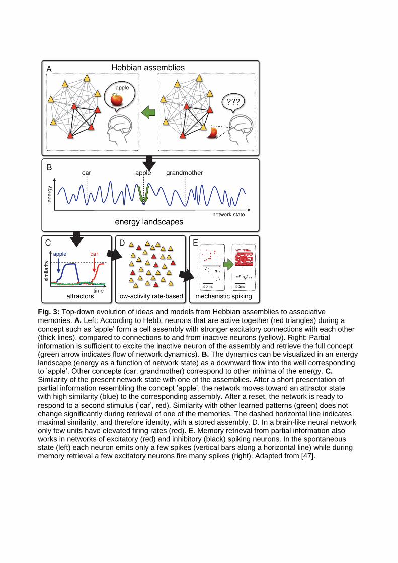
Fig. 3: Top-down evolution of ideas and models from Hebbian assemblies to associative memories. A. Left: According to Hebb, neurons that are active together (red triangles) during a concept such as ’apple’ form a cell assembly with stronger excitatory connections with each other (thick lines), compared to connections to and from inactive neurons (yellow). Right: Partial information is sufficient to excite the inactive neuron of the assembly and retrieve the full concept (green arrow indicates flow of network dynamics). B. The dynamics can be visualized in an energy landscape (energy as a function of network state) as a downward flow into the well corresponding to ’apple’. Other concepts (car, grandmother) correspond to other minima of the energy. C. Similarity of the present network state with one of the assemblies. After a short presentation of partial information resembling the concept ’apple’, the network moves toward an attractor state with high similarity (blue) to the corresponding assembly. After a reset, the network is ready to respond to a second stimulus (’car’, red). Similarity with other learned patterns (green) does not change significantly during retrieval of one of the memories. The dashed horizontal line indicates maximal similarity, and therefore identity, with a stored assembly. D. In a brain-like neural network only few units have elevated firing rates (red). E. Memory retrieval from partial information also works in networks of excitatory (red) and inhibitory (black) spiking neurons. In the spontaneous state (left) each neuron emits only a few spikes (vertical bars along a horizontal line) while during memory retrieval a few excitatory neurons fire many spikes (right). Adapted from [47].