prepared in cooperation with the maine geological survey · marcia k. mcnutt, director u.s....
TRANSCRIPT

U.S. Department of the InteriorU.S. Geological Survey
Scientific Investigations Report 2011–5227
Prepared in cooperation with the Maine Geological Survey
Simulation of Groundwater Conditions and Streamflow Depletion to Evaluate Water Availability in a Freeport, Maine, Watershed

Cover. Map of modeled area for Freeport aquifer groundwater-flow model, showing stream network, deep aquifer area (darker color), and shallow aquifer area (light color) in Freeport, Maine.

Simulation of Groundwater Conditions and Streamflow Depletion to Evaluate Water Availability in a Freeport, Maine, Watershed
By Martha G. Nielsen and Daniel B. Locke
Prepared in cooperation with the Maine Geological Survey
Scientific Investigations Report 2011–5227
U.S. Department of the InteriorU.S. Geological Survey

U.S. Department of the InteriorKEN SALAZAR, Secretary
U.S. Geological SurveyMarcia K. McNutt, Director
U.S. Geological Survey, Reston, Virginia: 2012
For more information on the USGS—the Federal source for science about the Earth, its natural and living resources, natural hazards, and the environment, visit http://www.usgs.gov or call 1–888–ASK–USGS.
For an overview of USGS information products, including maps, imagery, and publications, visit http://www.usgs.gov/pubprod
To order this and other USGS information products, visit http://store.usgs.gov
Any use of trade, product, or firm names is for descriptive purposes only and does not imply endorsement by the U.S. Government.
Although this report is in the public domain, permission must be secured from the individual copyright owners to reproduce any copyrighted materials contained within this report.
Suggested citation:Nielsen, M.G., and Locke, D.B., 2012, Simulation of groundwater conditions and streamflow depletion to evaluate water availability in a Freeport, Maine, watershed: U.S. Geological Survey Scientific Investigations Report 2011–5227, 72 p., at http://pubs.usgs.gov/sir/2011/5227/.

iii
Acknowledgments
Richard Knowlton of AquaAmerica and AquaMaine was generous in sharing information on water use and hydrogeologic data. Robert Gerber, of Ransom Environmental Consultants, kindly shared many unpublished reports and drilling records on the geology and hydrology of the Freeport aquifer.

THIS PAGE INTENTIONALLY LEFT BLANK

v
Contents
Abstract ...........................................................................................................................................................1Introduction.....................................................................................................................................................2
Purpose and Scope ..............................................................................................................................4Description of Study Area ...................................................................................................................4
Hydrogeologic Framework ...........................................................................................................................4Geology ...................................................................................................................................................4
Surficial Geology and Mapped Soils ........................................................................................5Glacial Geology at Depth ............................................................................................................5Bedrock .........................................................................................................................................5
Groundwater Resources .....................................................................................................................7Hydraulic Properties .................................................................................................................10Groundwater Flow .....................................................................................................................11
Recharge ............................................................................................................................11Groundwater Levels .........................................................................................................11
Surface-Water Resources ................................................................................................................13Streamflow Measurements in Harvey and Merrill Brooks .................................................14
Conceptual Model of the Groundwater Flow System ...................................................................14Water Use and Withdrawals ......................................................................................................................16
Reported Withdrawals from the Freeport Aquifer ........................................................................16Estimated Withdrawals from Groundwater ....................................................................................16
Simulation of Groundwater Flow and Discharge to Streams ...............................................................17Steady-State Numerical Groundwater-Flow Model .....................................................................17
Spatial Discretization of the Model ........................................................................................18Boundary Conditions .................................................................................................................18Stresses .......................................................................................................................................18Hydraulic Properties .................................................................................................................21
Model Calibration Using Parameter Estimation and Observations ............................................21Observations ...............................................................................................................................24Parameters..................................................................................................................................26Changes to the Conceptual Model .........................................................................................26Model Fit to Observations ........................................................................................................30Simulated Groundwater Levels and Flow Under Steady-State Conditions .....................32Model Sensitivity Analysis and Parameter Uncertainty .....................................................32Limitations of the Model ...........................................................................................................40
Model-Calculated Water Budget for Harvey and Merrill Brooks and the Buried Freeport Aquifer ....................................................................................................................40
Evaluation of Streamflow Depletion in Harvey Brook ...........................................................................42Calculation of Instream Flow Requirements for Harvey Brook ...................................................45Streamflow Depletion Estimates Based on STRMDEPL08 ..........................................................45Simulation of Streamflow Depletion Based on the Steady-State Groundwater-
Flow Model .............................................................................................................................48Comparison of Methods Used to Evaluate Streamflow Depletion ....................................50Comparison of Streamflow Depletion Estimates to Instream Flow Requirements .........50

vi
Figures 1. Map showing location of watersheds in the Freeport aquifer study area, Maine ............3 2. Map showing buried valley extent, showing altitude of bedrock in wells and
interpolated bedrock surface altitude, Freeport, Maine ........................................................6 3. Map showing interpreted surficial geology of the Freeport aquifer study area ................8 4. Geologic cross sections A–A’, B–B’, and C–C’ in the Freeport aquifer study area ...........9 5. Map showing groundwater level and streamflow measurement sites in the
Freeport aquifer study area ......................................................................................................12 6. Graphs showing A, streamflow measurements in Harvey and Merrill Brooks, and
B, precipitation in Portland, Maine, May–September 2009 .................................................15 7. Graph showing estimates of monthly mean streamflow at the Harvey and Merrill
Brook sites based on data from long-term index sites in southern Maine and New Hampshire ..........................................................................................................................15
8. Model grid and boundary conditions for the Freeport aquifer groundwater-flow model ............................................................................................................................................19
9. Vertical cross section of the Freeport aquifer groundwater-flow model, row 65 ............20 10. Map showing recharge rates applied to the numerical model of the Freeport aquifer
study area ....................................................................................................................................22 11. Maps showing calibrated horizontal hydraulic conductivities (Kh) used in the
Freeport aquifer groundwater-flow model .............................................................................23 12. Maps showing calibrated vertical hydraulic conductivities (Kv) used in the
Freeport aquifer groundwater-flow model .............................................................................27 13. Map showing drain hydraulic conductivity values (Kdr) used in calibrated model..........28 14. Map showing groundwater level and streamflow measurement observations in the
Freeport aquifer study area, Maine .........................................................................................29 15. Graphs showing relation between observed and model-calculated values for
A, heads, and B, early summer streamflow, for the Freeport aquifer groundwater- flow model ....................................................................................................................................31
16. Scatterplot showing weighted residuals and unweighted simulated values for heads in the Freeport aquifer groundwater-flow model ......................................................32
17. Map showing spatial distribution of weighted residuals across the domain of the Freeport aquifer groundwater-flow model .............................................................................33
18. Boxplot showing ninety-five percent confidence intervals on steady-state streamflow simulation for the five streamflow sites in the Freeport aquifer study area ....................................................................................................................................35
19. Map showing steady-state simulated groundwater levels in layer 1, Freeport aquifer model area .....................................................................................................................36
20. Map showing steady-state simulated groundwater levels in layer 3, Freeport aquifer model area .....................................................................................................................37
21. Map showing steady-state simulated streamflow (groundwater discharge) from drain cells and drain observation zones in the Freeport aquifer model area ...................38
Suggestions for Improving Methods of Study for Water Availability ..................................................52Summary and Conclusions .........................................................................................................................53References Cited..........................................................................................................................................55Appendix 1. List of Wells and Observations Used in the Freeport Aquifer Study ..........................59Appendix 2. Details of Groundwater Model Calibration ....................................................................67

vii
22. Boxplots showing parameter estimates, 95-percent confidence intervals, and reasonable ranges for A, hydraulic conductivity and B, recharge parameters for the Freeport aquifer groundwater-flow model .............................................................................39
23. Graph showing steady-state simulated inflows and outflows for three subareas within the Freeport aquifer groundwater-flow system.........................................................42
24. Graph showing simulated water budget components under various hydrologic scenarios, including no pumping, decreased recharge, and increases in pumping for the Freeport aquifer groundwater-flow model ................................................................43
25. Graphs showing monthly median flow estimates, pumping, and instream flow requirements for A, Merrill Brook, and B, Harvey Brook, Freeport, Maine .....................46
26. Graph showing Harvey Brook median flow estimates and 90-percent prediction intervals ........................................................................................................................................47
27. Map showing steady-state calculated streamflow depletion in each drain cell in the Freeport aquifer groundwater-flow model ......................................................................49
28. Boxplot showing ninety-five-percent confidence intervals for simulated streamflow depletion caused by pumping for the Harvey and Merrill Brook sites ..............................50
29. Boxplot showing steady-state streamflow projections from the groundwater model for Harvey and Merrill Brooks for pumping and recharge scenarios, showing the 95-percent confidence intervals ..............................................................................................51
30. Graph showing summer streamflows, pumping, instream flow requirements and projections of streamflow depletion in Harvey Brook at site #1, Freeport, Maine ..........52
Tables 1. Hydraulic properties of hydrogeologic units in the Freeport Aquifer study area ............10 2. Streamflow site information, Harvey and Merrill Brook, 2009 ............................................13 3. Water users in Harvey and Merrill Brook watersheds, as reported by
HarrisInfosource, and personal reconnaissance .................................................................17 4. Estimated total withdrawals from groundwater by water use category in the
Harvey and Merrill Brook watersheds, 2009 ..........................................................................17 5. Hydrogeologic units and associated calibrated hydraulic conductivities .......................24 6. Observations used in calibration of the Freeport aquifer groundwater flow model,
with variance and weights for optimization used for each observation. ..........................25 7. Drawdown observed in layer 3 wells during pumping tests, and model-calculated
steady-state drawdown from pumping in the AquaMaine production wells ...................34 8. Steady-state model calculated and observed early summer streamflows in the
Freeport aquifer groundwater model ......................................................................................34 9. Steady-state model calculated annual water budget for the Freeport aquifer
groundwater-flow model and three subareas .......................................................................41 10. Simulated water budgets for the Freeport aquifer groundwater-flow model and
subareas under alternative hydrologic conditions ...............................................................44 11. Sensitivity analysis of STRMDEPL08 streamflow depletion evaluations for the
Freeport aquifer, based on reasonable ranges for unknown variables ............................48 12. Model-calculated streamflow depletion at each streamflow measurement site ...........48 13. Model-calculated streamflow and streamflow depletion in Harvey Brook and
Merrill Brook under various pumping and recharge scenarios .........................................51

viii
Conversion Factors, Datum, and Acronyms
Inch/Pound to SI
Multiply By To obtain
Length
inch (in) 2.54 centimeter (cm)foot (ft) 0.3048 meter (m)mile (mi) 1.609 kilometer (km)
Area
square mile (mi2) 2.590 square kilometer (km2)Volume
gallon (gal) 3.785 liter (L)million gallons (Mgal) 3,785 cubic meter (m3)
Flow rate
cubic foot per second (ft3/s) 0.02832 cubic meter per second (m3/s)cubic foot per day (ft3/d) 0.02832 cubic meter per day (m3/d)gallon per minute (gal/min) 0.06309 liter per second (L/s)gallons per day (gal/d) 0.003785 cubic meter per day (m3/d)million gallons per day (Mgal/d) 0.04381 cubic meter per second (m3/s)million gallons per year (Mgal/yr) 3,785 cubic meter per year (m3/yr)inch per year (in/yr) 25.4 millimeter per year (mm/yr)
Hydraulic conductivity
foot per day (ft/d) 0.3048 meter per day (m/d)Transmissivity*
foot squared per day (ft2/d) 0.09290 meter squared per day (m2/d)
Temperature in degrees Fahrenheit (°F) may be converted to degrees Celsius (°C) as follows: °C=(°F–32)/1.8
Vertical coordinate information is referenced to the North American Vertical Datum of 1988 (NAVD 88).
Horizontal coordinate information is referenced to the North American Datum of 1983 (NAD 83).
Altitude, as used in this report, refers to distance above the vertical datum.
*Transmissivity: The standard unit for transmissivity is cubic foot per day per square foot times foot of aquifer thickness [(ft3/d)/ft2]ft. In this report, the mathematically reduced form, foot squared per day (ft2/d), is used for convenience.
AcronymsMGS Maine Geological Survey
USGS U.S. Geological Survey
WRPC (Maine) Water Resources Planning Committee
AbstractIn order to evaluate water availability in the State of
Maine, the U.S. Geological Survey (USGS) and the Maine Geological Survey began a cooperative investigation to provide the first rigorous evaluation of watersheds deemed “at risk” because of the combination of instream flow require-ments and proportionally large water withdrawals. The study area for this investigation includes the Harvey and Merrill Brook watersheds and the Freeport aquifer in the towns of Freeport, Pownal, and Yarmouth, Maine. A numerical ground-water-flow model was used to evaluate groundwater withdraw-als, groundwater-surface-water interactions, and the effect of water-management practices on streamflow. The water budget illustrates the effect that groundwater withdrawals have on streamflow and the movement of water within the system.
Streamflow measurements were made following stan-dard USGS techniques, from May through September 2009 at one site in the Merrill Brook watershed and four sites in the Harvey Brook watershed. A record-extension technique was applied to estimate long-term monthly streamflows at each of the five sites.
The conceptual model of the groundwater system consists of a deep, confined aquifer (the Freeport aquifer) in a buried valley that trends through the middle of the study area, cov-ered by a discontinuous confining unit, and topped by a thin upper saturated zone that is a mixture of sandy units, till, and weathered clay. Harvey and Merrill Brooks flow southward through the study area, and receive groundwater discharge from the upper saturated zone and from the deep aquifer through previously unknown discontinuities in the confining unit. The Freeport aquifer gets most of its recharge from local seepage around the edges of the confining unit, the remainder is received as inflow from the north within the buried valley.
Groundwater withdrawals from the Freeport aquifer in the study area were obtained from the local water utility and estimated for other categories. Overall, the public-supply withdrawals (105.5 million gallons per year (Mgal/yr)) were much greater than those for any other category, being almost 7 times greater than all domestic well withdrawals (15.3 Mgal/yr). Industrial withdrawals in the study area (2.0 Mgal/yr) are mostly by a company that withdraws from an aquifer at the edge of the Merrill Brook watershed. Commercial withdrawals are very small (1.0 Mgal/yr), and no irrigation or other agricultural withdrawals were identified in this study area.
A three-dimensional, steady-state groundwater-flow model was developed to evaluate stream-aquifer interactions and streamflow depletion from pumping, to help refine the conceptual model, and to predict changes in streamflow result-ing from changes in pumping and recharge. Groundwater lev-els and flow in the Freeport aquifer study area were simulated with the three-dimensional, finite-difference groundwater-flow modeling code, MODFLOW-2005. Study area hydrology was simulated with a 3-layer model, under steady-state conditions.
The groundwater model was used to evaluate changes that could occur in the water budgets of three parts of the local hydrologic system (the Harvey Brook watershed, the Merrill Brook watershed, and the buried aquifer from which pumping occurs) under several different climatic and pumping scenarios. The scenarios were (1) no pumping well with-drawals; (2) current (2009) pumping, but simulated drought conditions (20-percent reduction in recharge); (3) current (2009) recharge, but a 50-percent increase in pumping well withdrawals for public supply; and (4) drought conditions and increased pumping combined. In simulated drought situations, the overall recharge to the buried valley is about 15 percent less and the total amount of streamflow in the model area is reduced by about 19 percent. Without pumping, infiltration to the buried valley aquifer around the confining unit decreased by a small amount (0.05 million gallons per day (Mgal/d)), and discharge to the streams increased by about 8 percent (0.3 Mgal/d). A 50-percent increase in pumping resulted in a simulated decrease in streamflow discharge of about 4 percent (0.14 Mgal/d).
Simulation of Groundwater Conditions and Streamflow Depletion to Evaluate Water Availability in a Freeport, Maine, Watershed
By Martha G. Nielsen1 and Daniel B. Locke2
1U.S. Geological Survey.2Maine Geological Survey.

2 Groundwater Conditions and Streamflow Depletion to Evaluate Water Availability in a Freeport, Maine, Watershed
Streamflow depletion in Harvey Brook was evaluated by use of the numerical groundwater-flow model and an analyti-cal model. The analytical model estimated negligible depletion from Harvey Brook under current (2009) pumping conditions, whereas the numerical model estimated that flow to Harvey Brook decreased 0.38 cubic feet per second (ft3/s) because of the pumping well withdrawals. A sensitivity analysis of the analytical model method showed that conducting a cursory evaluation using an analytical model of streamflow depletion using available information may result in a very wide range in results, depending on how well the hydraulic conductivity variables and aquifer geometry of the system are known, and how well the aquifer fits the assumptions of the model. Using the analytical model to evaluate the streamflow depletion with an incomplete understanding of the hydrologic system gave results that seem unlikely to reflect actual streamflow deple-tion in the Freeport aquifer study area.
In contrast, the groundwater-flow model was a more robust method of evaluating the amount of streamflow deple-tion that results from withdrawals in the Freeport aquifer, and could be used to evaluate streamflow depletion in both streams. Simulations of streamflow without pumping for each measurement site were compared to the calibrated-model streamflow (with pumping), the difference in the total being streamflow depletion. Simulations without pumping resulted in a simulated increase in the steady-state flow rate of 0.38 ft3/s in Harvey Brook and 0.01 ft3/s in Merrill Brook. This translates into a streamflow-depletion amount equal to about 8.5 percent of the steady-state base flow in Harvey Brook, and an unmeasurable amount of depletion in Merrill Brook. If pumping was increased by 50 percent and recharge reduced by 20 percent, the amount of streamflow depletion in Harvey Brook could reach 1.41 ft3/s.
IntroductionIn 2007, the State of Maine established the Maine Water
Resources Planning Committee (WRPC), whose mandate is to plan for the sustainable use of water resources in the State. The WRPC gathers water-resources data, analyzes watershed withdrawals relative to instream flow requirements, and provides guidance and tools for State and local governments with respect to water availability and managing water resources. The State uses estimates of natural monthly flows, sometimes combined with site-specific geomorphic analysis, to evaluate streamflow requirements in support of aquatic habitat when a proportionally large withdrawal is identified in a watershed. The instream flow requirements are specific to six time periods—winter (January 1 to March 15), spring (March 16 to May 15), early summer (May 16 to June 30), summer (July 1 to September 15), fall (September 16 to November 15), and early winter (November 16 to December 31)—each of which is based on estimates of median monthly streamflows.
Although information on large water withdrawals is well coordinated among State agencies, there is no consistently
applied method for tracking the sum of water withdrawals in a watershed, and assessing the potential effects of those withdrawals on streamflows. In addition, to better implement the instream flow requirements, further insight into the effects of groundwater withdrawals on the overall water budget and natural streamflows in watersheds with high withdrawals is needed in the state.
The WRPC, through the lead of the Maine Geological Survey (MGS), desires to conduct additional investigations into watersheds deemed “at risk” because of the combination of instream flow requirements and proportionally large water withdrawals. These additional investigations are intended to provide in-depth analyses of the hydrologic systems and water budgets to determine first, whether certain watersheds are indeed approaching their withdrawal limit and second, to better understand the potential effect of withdrawals on aquatic base flows and the overall hydrologic system. The MGS identified two adjacent watersheds in the Freeport, Maine, area (fig. 1) as having a permitted withdrawal from pumping wells for public water supply in combination with flows required to meet instream flow requirements that are quite large in comparison to the total annual runoff. These watersheds (Harvey and Merrill Brook) and the Freeport aquifer, from which water is withdrawn, serve as the study area to illustrate the issues just identified. This study area provides an example of the hydrologic processes and effects that pumping well withdrawals can have on a small (less than 10 square miles (mi2)) watershed.
In 2009, the U.S. Geological Survey (USGS) and the MGS cooperatively began the first rigorous evaluation (or pilot study) of the hydrologic effects of withdrawals in “water-sheds at risk.” The study has three goals related to evaluating water availability in watersheds with large withdrawals:
• Provide a blueprint for estimating total withdrawals in a watershed, both reported and unreported;
• Evaluate the current and future potential water-management scenarios in a watershed to assist water-resource managers in making decisions about water-supply issues; and
• Evaluate the effect of withdrawals on streamflows and streamflow depletion in light of the State requirements to maintain instream flows for aquatic habitat protec-tion.
The use of a numerical groundwater-flow model to evalu-ate groundwater withdrawals allows water to be accounted for as it flows through the groundwater system to the surface-water system, and provides a method to evaluate the effect of water-management practices on streamflow. The Freeport aquifer groundwater-flow model (hereafter referred to as “the groundwater-flow model” or “the model”) was also used to help refine the conceptual model of groundwater flow in the study area, because the possible source(s) of groundwater to the withdrawal wells was poorly understood at the outset.

Introduction 3
!
!
!
295
MAINE
Study area
Bangor
Augusta
Portland
Merrill Brook
Harvey BrookHarvey Brook
Freeport
Pownal
Yarmouth
North Yarmouth Merrill
Brook
Harvey Brook
Cous
ins R
iver
Harra
seek
et Ri
ver
FreeportFreeportn
70°06'70°08'70°10'
43°52'
43°50'
Base from U.S. Geological Survey digital data, 1:24,000Universal Transverse Mercator projection, Zone 19NCentral meridian -69°Shaded relief from U.S. Geological Survey National ElevationDataset 10-meter digital elevation modelNorth American Datum of 1983 (NAD 83)
0 21 MILES
0 21 KILOMETERS
EXPLANATION
Study area watershed boundary
Figure 1. Location of watersheds in the Freeport aquifer study area, Maine.

4 Groundwater Conditions and Streamflow Depletion to Evaluate Water Availability in a Freeport, Maine, Watershed
Purpose and Scope
This report documents the simulation of streamflow conditions and groundwater depletion for two adjacent small watersheds (Harvey Brook and Merrill Brook) in southeastern Maine. Specifically, the report describes the determination of total water use and withdrawals, the use and calibration of a steady-state groundwater-flow model of the Freeport aquifer, and its use in evaluating the effect of groundwater withdrawals on streamflow. The data collected to construct and calibrate the groundwater-flow model are presented. Simulation results for varying water withdrawal and climatic scenarios on the water budgets for the Freeport aquifer, Harvey Brook, and Merrill Brook are described. The parameter estimation used for model calibration, model sensitivities and limitations, and prediction uncertainties also are reported for the model. In addition to the groundwater-flow model, the report describes the use of a program, STRMDEPL08, which uses analytical solutions to evaluate streamflow depletion in Harvey Brook. The report presents a summary of the effect of withdrawals on streamflows in the study area, and on the overall movement of water through the hydrologic system. Finally, suggestions for conducting future studies are presented.
Description of Study Area
The study area includes the Harvey Brook and Merrill Brook watersheds and the Freeport aquifer, which lies within the Harvey and Merrill Brook watersheds beneath the towns of Freeport, Pownal, and Yarmouth, Maine (fig. 1). The aquifer was mapped initially as a significant sand and gravel aquifer by the Maine Geological Survey (Neil and Locke, 1999a, b). Studies commissioned by the AquaMaine–Freeport Division water utility, which is the primary user of water in the Freeport aquifer, refined the mapped extent of the aquifer, showing that it lies in a buried river valley (fig. 2) that does not specifically coincide with the surficial aquifer mapping, which was based largely on the extent of sandy soils in the area. The northern and southern limits of the aquifer have not been identified, but well data suggest that the buried valley extends southward under the Atlantic Ocean. The northern extent of the buried valley could extend outside the study area toward the Durham southwest bend of the Androscoggin River (Gerber, 1979). The Freeport aquifer, as referred to herein, constitutes the buried valley aquifer, often called the Harvey Brook aquifer in consulting reports, and is the subject of the modeling effort in this report along with the surficial sediments overlying the aquifer (fig. 2).
The study area has rolling topography, dissected by streams in valleys having slopes that range from shallow and gradual to steep. The relief is largely controlled by bedrock ridges, and valleys created by glacial action. Land surface altitude in the study area ranges from 0 to 220 feet (ft).
Harvey Brook and Merrill Brook join and become the Cousins River, which flows into the ocean approximately 2.5 miles (mi) southwest of their confluence. The Cousins
River is tidal along its entire length. Above the confluence at the Cousins River, the Harvey Brook watershed is 4.0 mi2 and the Merrill Brook watershed is 4.6 mi2, although the watershed areas for which data are compiled upstream from the streamflow measurement sites are slightly smaller (3.18 and 3.81 mi2, respectively).
The mean annual precipitation in the Freeport area for the 1961–1990 period is 45.9 inches (in.) (Oregon State University, 2010; Natural Resources Conservation Service, 1998). The closest long-term temperature station is in Portland, Maine, which is 15.5 mi southwest of Freeport along the coast. The average annual temperature for the Portland station is 45.7°F (National Weather Service, 2010), which is expected to be the same in the Freeport area, given their similar altitude, distance from the Atlantic Ocean, and proximity to each other. The land use in and around the study area is primarily rural residential, with the exception of the town centers of Freeport and Yarmouth, and the U.S. 1/Interstate-295 corridor, which is dominated by commercial development. The rural residential areas are largely forested, with interspersed hayfields along roadways and small areas of unbroken forest between adjacent roadways and residential corridors. The largest area of unbroken forest in the study area is in the center of the Harvey Brook watershed. The populations of Freeport and Yarmouth in 2000 were 7,800 and 8,360, respectively (U.S. Census Bureau, 2000), with population densities of 225 to 626 persons/mi2.
Hydrogeologic FrameworkThe highly productive portion of the Freeport aquifer
lies within the buried bedrock valley (fig. 2), which trends roughly north-south in the Freeport area (Gerber, 1979, 1985). The aquifer consists of layered sand, fine sand, silt, and gravel. Above these productive sediments, a silt and clay layer (known as the Presumpscot Formation (Bloom, 1960, 1963)) forms a discontinuous confining unit between the deep aquifer and sandy deposits at the surface. The Presumpscot Formation is thickest in the middle of the buried valley, but thins consid-erably at the valley edges, and is absent in parts. The bedrock hillsides adjacent to the buried valley are covered with a heterogeneous distribution of till, sand, and clay.
Geology
The geologic units in the study area include fractured crystalline bedrock and stratified, unconsolidated glacial deposits that are draped over the bedrock. The glacial depos-its include till (in moraines and as a blanket deposit), strati-fied marine sand and gravel, marine silt and clay, beach and nearshore sand and gravel deposits, and eolian sand deposits (Marvinney, 1999b; Retelle, 1999a, b; Weddle, 1999; Weddle and Retelle, 1995). More recent sediments include Holocene stream alluvium and Holocene wetlands.

Hydrogeologic Framework 5
Surficial Geology and Mapped SoilsAfter the last glacial maximum, the melting glacier
retreated northward past coastal Maine, leaving a number of deposits as the retreat occurred. The retreat was accompanied by a marine transgression onto the depressed land surface, so that sediments carried by the melting glacier were depos-ited in a shallow marine environment (Weddle and Retelle, 1995). Unsorted sediment from the bottom of the glacier was deposited as till over the bedrock surface. Submarine meltwa-ter conduits transported coarse sediment out toward the sea, where it was deposited in submarine fans and deltas. In calm-water areas, finer grained sediments (silt and clay) fell out of suspension onto the submarine surface, forming a widespread silt and clay layer known as the Presumpscot Formation (Bloom, 1960, 1963). As the glacier retreated farther inland, the land surface rebounded, exposing the marine sediments first to wave action, and then to subaerial erosion and deposi-tion. During this phase, the top layer of marine sediments was reworked by wave action, leaving widespread nearshore sandy deposits over the silt and clay (Weddle and Retelle, 1995). Wind and water further reworked these sediments, exposing till uplands, creating eolian sand deposits, and filling in stream valleys with alluvial deposits.
The surficial materials and surficial geology maps show areas of thin drift, where the depth to bedrock is very shallow, and locations of bedrock outcrop. The surficial geology map for the Freeport quadrangle does not differentiate sandy areas from silt and clay areas within one of the surficial geologic units, which required the use of additional sources and some field investigation for this study. The interpreted surficial geology in the study area is shown in figure 3; this map represents a combination of surficial geology mapped by the Maine Geological Survey (Marvinney, 1999a, b; Retelle, 1999a, b), soils (Natural Resources Conservation Service, 2006), and field observations. The stratigraphically uppermost units are the eolian sands and nearshore marine deposits, which generally overlie the silt and clay of the Presumpscot Formation. (Sandy deposits overlying the silt and clay of the Presumpscot Formation have often been identified as an upper nearshore sand facies of the formation, but have sometimes been found to unconformably overlie the silt and clay (Weddle and Retelle, 1995); figure 3 shows the sandy deposits as a separate unit.) The largest area of eolian sand lies in the middle of the Harvey Brook watershed. To the north and south along Harvey Brook, and to the east of these eolian sands, sandy soils (interpreted as being the same as mapped nearshore marine sands in the north part of the study area) are widespread. An area of soils described as consisting of sand, gravel, and boulders is exposed at the surface on the western side of Harvey Brook. This bouldery, sandy unit can be found exposed in gullies leading into the valley of Harvey Brook, and has been observed to be a zone in which runoff from rainfall events is absorbed into the subsurface.
The Presumpscot Formation silt and clay lies stratigraphi-cally beneath the eolian sands and sandy nearshore sediments.
Gerber and Hebson (1996) describe the Presumpscot Forma-tion as follows:
“The Presumpscot Formation clay-silt is typically composed of about 10 ft of desiccated brown and olive clay-silt overlying a softer “blue” or gray silt-clay. The desiccated zone is fissured into a suban-gular block pattern, more dense and closely spaced at the ground surface and diminishing at depth. The softer gray clay lies below the position of the perma-nent water table.”Till is the stratigraphically lowest glacial unit in the study
area, and directly overlies the bedrock. The till is sandy, dense, and is often shown as being about 5 ft in thickness in drillers logs in the area. In addition, There are many areas in which the glacial deposits are very thin, and these have been mapped as thin till or undifferentiated thin glacial deposits (fig. 3). Holocene alluvium and wetlands can be found in many of the stream valleys in the study area.
Glacial Geology at DepthThe available surficial geology maps do not show the
overall thickness and stratigraphy of the entire suite of glacial deposits in the study area. The Freeport aquifer lies beneath an area that is mapped as Presumpscot Formation and sandy eolian and nearshore deposits at the surface. Well logs from (1) the Maine Geological Survey’s well driller’s database, (2) seismic refraction lines, (3) well and boring logs from numerous studies commissioned by the AquaMaine–Freeport Division water utility (Weston Geophysical (1973), Maine Water Company (1978), Hydro Group (1984, 1988, 1991, 1992, 1995, 1997), Caswell, Eichler, and Hill (1993, 1994), Gerber (1979, 1980, 1985, 1995), Gerber-Jacques Whitford (1996), Stratex (1999, 2001a, b, 2002, 2003), Drumlin Environmental (2000), Sevee & Maher (2002), Reynolds (2000), Earth Tech (2004), URS Corporation (2002), and R.E. Chapman Company (2003), and (4) logs of two wells drilled for this study collectively indicate that a buried valley lies beneath the Harvey Brook watershed and extends for an indeterminate distance to the north and south of the study area (fig. 2). The sediments at depth consist of layered coarse sand, fine gravel, fine sand, and silt, which indicates that this buried valley probably once served as a conduit for sediment-laden glacial meltwater flowing under a retreating glacier. All the wells and borings with data used for this study are listed in appendix 1.
BedrockBedrock in the study area consists of the Hutchins Corner
Formation, a biotite-quartz-plagioclase granofels metamorphic rock (Berry and Hussey, 1998). The bedrock surface was interpolated for the study from several sources of data. Drilling records for domestic (primarily bedrock) wells were obtained for the study area from the Maine Geological Survey,

6 Groundwater Conditions and Streamflow Depletion to Evaluate Water Availability in a Freeport, Maine, Watershed
Harra
seek
et Ri
ver
EE
E
E
E
E
E
E
E
E
E
E
EEEEEEE
EEEE
EEEE
EE
E
E
E
EE
E
EE
EE
E
E
E
E
E E
EE
E
EE
E
E
E
EE
E
E
E
E
EE
EEEEEE
E
EEEEEE
EE
E E
EE
EEE EE
EE
EE
E
EE
E
EEEE E
EE
E
E
EEEEE
EE EE
Freeport
Pownal
Yarmouth
North Yarmouth Merr
ill Broo
k
Harvey
Brook
-15
-58
-37-36
-30 -79-16
0
5
9
9
1
7613
5559
31
95
77
80
54
8251
31 -8
-6
44
-5
153830
3643
45
-3-9
23
15 67
-95-99
-57
-29
-24
-40
-25
-25
-36-31
-32
-12-56
-17
-16
-24-48-57
-79
-31
-48
-41
-77
-76
-118
-113
70°8'70°10'
43°52'
43°50'
43°48' ?
??
Base from U.S. Geological Survey digital data, 1:24,000Universal Transverse Mercator projection, Zone 19NCentral meridian -69°Shaded relief from U.S. Geological Survey National ElevationDataset 10-meter digital elevation modelNorth American Datum of 1983 (NAD 83)
Geology modified from Maine Geological SurveySurficial Geology maps 1:24,000
0 10.5 MILE
0 10.5 KILOMETER
Area of inset
EXPLANATION
Buried valley extent
Well or boring in buried valley showing altitude of bedrock—In feet
E Bedrock outcrop
Area of uncertain extent?
Active model area
295
Cous
ins R
iver
38
Figure 2. Buried valley extent, showing altitude of bedrock in wells and interpolated bedrock surface altitude, Freeport, Maine.

Hydrogeologic Framework 7
and typically include depth to bedrock, total well depth, and well yield. Seismic profiles from Weston Geophysical (1973) and Caswell, Eichler, and Hill (1994), and the Maine Geological Survey (Neil and Locke, 1999a, b, 2002) indicate depth to bedrock in many areas. Additional well logs from consulting reports (listed previously) were also consulted to determine the bedrock surface at depth.
Groundwater Resources
Groundwater available to wells occurs in four hydro-geologic units in the Freeport area. Although water within the fractured crystalline bedrock underlying all the surficial units is utilized as a water source for domestic wells, the low yields typically obtained from these wells limit this source to small, domestic uses. Where it overlies the bedrock in upland areas, water-containing till is used as a water supply for dug wells. The deep sand and gravel deposits in the buried valley under Harvey Brook (fig. 2) compose the Freeport aquifer. This
aquifer consists of layered fine and silty fine sand containing lenses of coarse clean sand, with the most transmissive layers being about 20–30 ft thick. Finally, sandy deposits at the sur-face can hold significant amounts of water and provide water to dug wells and springs that are used for domestic water supplies. Stratigraphically separating the surficial sands from the deep sand and gravel deposits, the Presumpscot Forma-tion acts as a discontinuous confining layer above the Freeport aquifer.
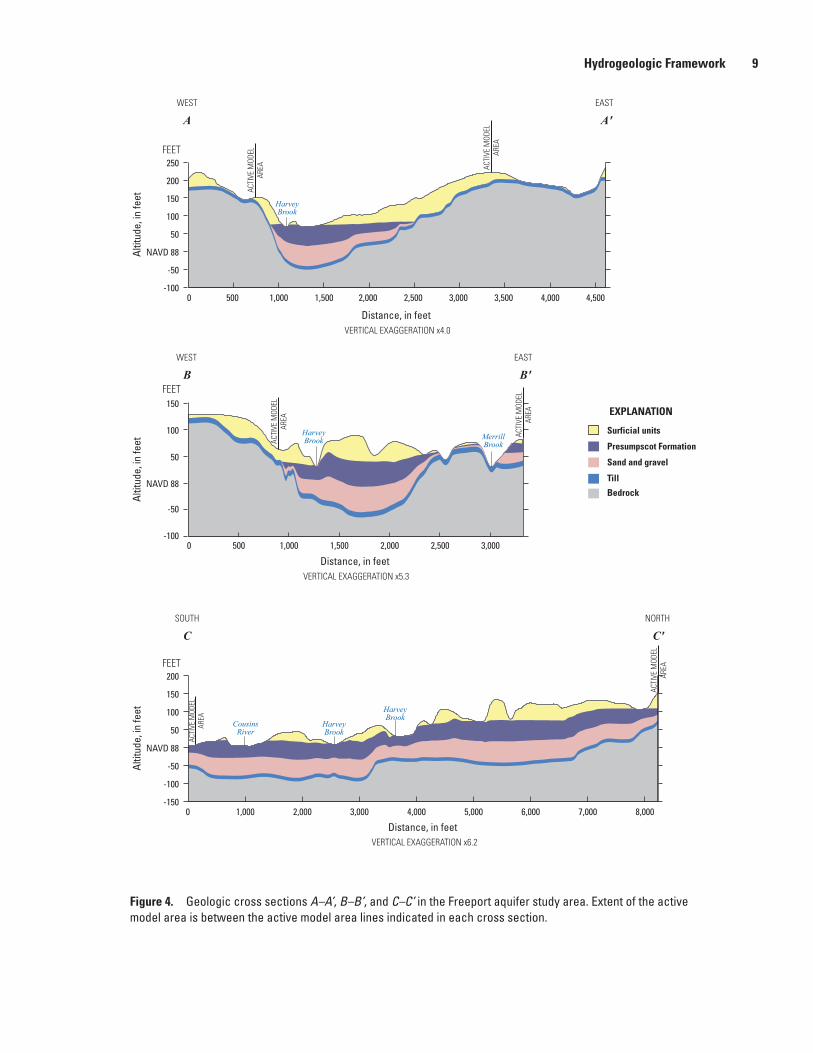
Hilltops with thin till cover and undifferentiated thin glacial deposits present opportunities for recharge to the bedrock aquifer, and to the buried sand and gravel deposit underneath the confining layer. Figure 4 shows three cross sections across the study area, two from west to east (A–A’ and B–B’), and one from south to north along the buried valley (C–C’). Each cross section shows the following, from top to bottom: (1) land surface; (2) the top of the confining Presumpscot Formation, interpolated across the study area from well logs and surface exposures; (3) the bottom of the Presumpscot Formation (the line indicating the base of
Altitude of bedrock—In feet
High: 220
Low: -95
EXPLANATION
Figure 2. Buried valley extent, showing altitude of bedrock in wells and interpolated bedrock surface altitude, Freeport, Maine.—Continued

8 Groundwater Conditions and Streamflow Depletion to Evaluate Water Availability in a Freeport, Maine, Watershed
E
E
E
E
E
E
E
E
E
E E
EEE
E
EE
E
E
E
E
EE
EEEEE
EEEEEE
EE
C'
C
A
A'
B'
B
Freeport
Pownal
Yarmouth
North Yarmouth
Harvey Brook
Merrill
Broo
k
70°08'70°10'
43°52'
43°50'
0 10.5 MILE
0 1 20.5 KILOMETERS
Geology modified from Maine Geological SurveySurficial Geology maps 1:24,000
Geology mapped by C.L. Marvinney (1999), T. Weddle (1999),and M. Retelle (1999), and modified by M. Nielsen in 2009
Base from U.S. Geological Survey digital data, 1:24,000Universal Transverse Mercator projection, Zone 19NCentral meridian -69°North American Datum of 1983 (NAD 83)
EXPLANATION
Till
Thin till—Less than 10 feet to bedrock
Gravel pit
Mapped marine nearshore
Sand at surface—Nearshore marine
Mapped marine shoreline
Eolian sand—Mostly above clay
Upland area
Valley bottom
Sand, gravel, boulders
Silty alluvium (Holocene)
Thin drift—Undifferentiated
Wetland
Active model area
Cross-section trace
Bedrock outcrop
Presumpscot Formation
E
A A'
295
Figure 3. Interpreted surficial geology of the Freeport aquifer study area.
Hydrogeologic Framework 9
ACTI
VE M
ODEL
AREA
ACTI
VE M
ODEL
AREA
ACTI
VE M
ODEL
AREA
HarveyBrook
HarveyBrook Merrill
Brook
HarveyBrook
HarveyBrook
CousinsRiver
ACTI
VE M
ODEL
AREA
ACTI
VE M
ODEL
AREA
ACTI
VE M
ODEL
AREA
CSOUTH NORTH
AWEST EAST
B
C'
A'
B'WEST EAST
-100
-50
NAVD 88
50
100
150
200
250FEET
FEET
FEET
Altit
ude,
in fe
et
Distance, in feet
Distance, in feet
Distance, in feet
Altit
ude,
in fe
etAl
titud
e, in
feet
0 500 1,000 1,500 2,000 2,500 3,000 3,500 4,000 4,500
-100
-50
NAVD 88
50
100
150
0 500 1,000 1,500 2,000 2,500 3,000
-150
-100
-50
NAVD 88
50
100
150
200
0 1,000 2,000 3,000 4,000 5,000 6,000 7,000 8,000
VERTICAL EXAGGERATION x4.0
VERTICAL EXAGGERATION x5.3
VERTICAL EXAGGERATION x6.2
Surficial units
Presumpscot Formation
Sand and gravel
Till
Bedrock
EXPLANATION
Figure 4. Geologic cross sections A–A’, B–B’, and C–C’ in the Freeport aquifer study area. Extent of the active model area is between the active model area lines indicated in each cross section.
10 Groundwater Conditions and Streamflow Depletion to Evaluate Water Availability in a Freeport, Maine, Watershed
the confining layer shown in figure 4 represents an average thickness of the Presumpscot Formation from available well logs); (4) a layer representing a uniform 10-ft thick layer of till above the bedrock, which is present at the bottom of most well logs in the study area; and (5) the bedrock. The surface representing the top of the bedrock is interpolated from well data.
Harvey and Merrill Brooks flow in valleys incised into the surficial materials. Merrill Brook flows in a basin that is dominated by fine-grained soils (till, silt, and clay). The Harvey Brook valley is more deeply incised into the surficial units. The steep valley sides of Harvey Brook are sandy at the top and transition into the silt/clay of the Presumpscot Formation near the bottom. Holocene alluvium, consisting of fine sand and silt, fills the bottom of the stream valleys (not shown in fig. 4). Outcrops of layered silt/clay are often exposed on the outside meander curve of the streambed, and in places within the bottom of the streambed.
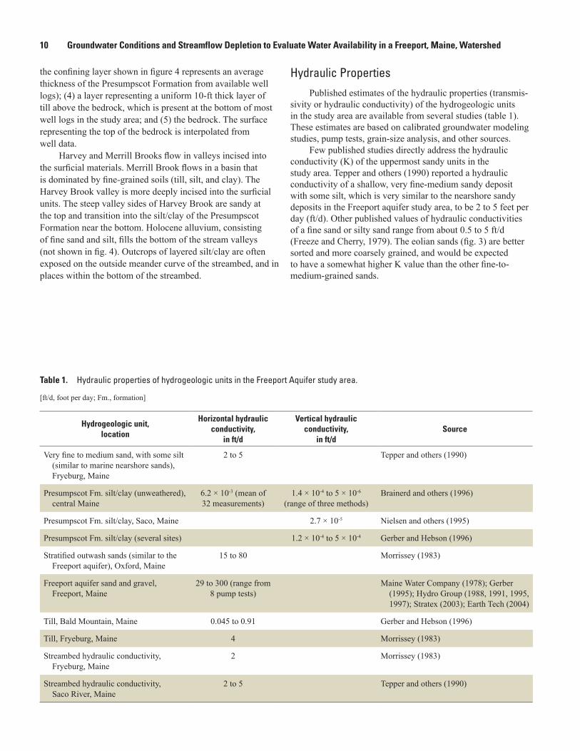
Hydraulic PropertiesPublished estimates of the hydraulic properties (transmis-
sivity or hydraulic conductivity) of the hydrogeologic units in the study area are available from several studies (table 1). These estimates are based on calibrated groundwater modeling studies, pump tests, grain-size analysis, and other sources.
Few published studies directly address the hydraulic conductivity (K) of the uppermost sandy units in the study area. Tepper and others (1990) reported a hydraulic conductivity of a shallow, very fine-medium sandy deposit with some silt, which is very similar to the nearshore sandy deposits in the Freeport aquifer study area, to be 2 to 5 feet per day (ft/d). Other published values of hydraulic conductivities of a fine sand or silty sand range from about 0.5 to 5 ft/d (Freeze and Cherry, 1979). The eolian sands (fig. 3) are better sorted and more coarsely grained, and would be expected to have a somewhat higher K value than the other fine-to-medium-grained sands.
Table 1. Hydraulic properties of hydrogeologic units in the Freeport Aquifer study area.
[ft/d, foot per day; Fm., formation]
Hydrogeologic unit, location
Horizontal hydraulic conductivity,
in ft/d
Vertical hydraulic conductivity,
in ft/dSource
Very fine to medium sand, with some silt (similar to marine nearshore sands), Fryeburg, Maine
2 to 5 Tepper and others (1990)
Presumpscot Fm. silt/clay (unweathered), central Maine
6.2 × 10⁻³ (mean of 32 measurements)
1.4 × 10⁻⁴ to 5 × 10⁻⁶ (range of three methods)
Brainerd and others (1996)
Presumpscot Fm. silt/clay, Saco, Maine 2.7 × 10⁻⁵ Nielsen and others (1995)
Presumpscot Fm. silt/clay (several sites) 1.2 × 10⁻⁴ to 5 × 10⁻⁴ Gerber and Hebson (1996)
Stratified outwash sands (similar to the Freeport aquifer), Oxford, Maine
15 to 80 Morrissey (1983)
Freeport aquifer sand and gravel, Freeport, Maine
29 to 300 (range from 8 pump tests)
Maine Water Company (1978); Gerber (1995); Hydro Group (1988, 1991, 1995, 1997); Stratex (2003); Earth Tech (2004)
Till, Bald Mountain, Maine 0.045 to 0.91 Gerber and Hebson (1996)
Till, Fryeburg, Maine 4 Morrissey (1983)
Streambed hydraulic conductivity, Fryeburg, Maine
2 Morrissey (1983)
Streambed hydraulic conductivity, Saco River, Maine
2 to 5 Tepper and others (1990)
Hydrogeologic Framework 11
Because of its regional importance as a confining unit, the Presumpscot Formation has been studied thoroughly. In addition to the sandy zone at its top, the Presumpscot Formation often has a weathered, desiccated zone about 10 ft in thickness above the softer, massive blue-gray clay and silt (Gerber and Hebson, 1996). This zone, which occurs in the unsaturated zone above the level of the local water table, is characterized by extensive fissuring and an olive-brown color. According to Gerber and Hebson (1996), this layer can have a hydraulic conductivity 50 times greater than the underlying saturated, unweathered silt/clay. Brainerd and others (1996) measured the horizontal and vertical hydraulic conductivity of the unweathered Presumpscot silt/clay at a site in central Maine using isotopic analysis and groundwater age dating. The reported horizontal K of the Presumpscot Formation was 6.2 × 10⁻³ ft/day and the vertical hydraulic conductivity of unweathered Presumpscot Formation was 1.4 × 10⁻⁴ to 5 × 10⁻⁶ ft/day. Nielsen and others (1995) reported a vertical K of the Presumpscot Formation of 2.7 × 10⁻⁵ ft/d, measured in an area south of Portland, Maine.
There have been numerous evaluations of the Freeport aquifer, particularly in the area within ½ mi of the pumping wells. Pump tests indicate a heterogeneous, stratified aquifer, with transmissivities that ranged from 650 to 13,000 square feet per day (ft2/d), corresponding to hydraulic conductivities ranging from 29 to 300 ft/d (Maine Water Company, 1978; Gerber, 1995; Hydro Group, 1984, 1988, 1991, 1995, 1997; Stratex, 2003; Earth Tech, 2004).
The till in the study area has not been studied directly, but evidence from a small number of studies in Maine and other sources (Morrissey, 1983; Gerber and Hebson, 1996; Freeze and Cherry, 1979) indicates that the K of the till could be 0.5 to 10 ft/d.
Groundwater FlowThis section describes the flow of groundwater in
the study area and, together with the description of the hydrogeologic units, forms the basis for the conceptual model described later.
Recharge
Recharge to the Freeport aquifer has not been measured directly, nor have the numerous consulting reports addressed specific recharge rates for the study area. The theoretical maximum amount of shallow recharge to sandy soils is about 25 inches per year (in/yr), based on the Lyford and Cohen (1988) method, or about 54 percent of precipitation. The sandy nearshore marine units and the eolian sands could, therefore, have recharge rates in the 22–25 in/yr range. Morrissey (1983) found that in a valley-fill sand and gravel aquifer, recharge from runoff from adjacent uplands was an important part of the water budget, and could be as much as 60 percent of the precipitation in upland areas. Recharge to till in other areas of Maine has been calculated or estimated to be 7.5 in/yr in
Oxford County (Morrissey, 1983); 5 to 5.5 in/yr in Washington County (Gerber and Hebson, 1996); 3.5 to 8 in/yr in Woodland, Maine (Gerber and Hebson, 1996); and 7 in/yr in the Bald Mountain area of Aroostook County (Fontaine, 1989). Published values of recharge into the Presumpscot Formation also have been summarized by Gerber and Hebson (1996). Recharge into the unweathered, saturated silt/clay ranges from less than 0.5 to 1.9 in/yr, whereas recharge into the weathered, fissured zone of the silt/clay could be as much as 12 in/yr (Gerber and Hebson, 1996). The presence of unsewered suburban housing developments could add to the total amount of recharge entering the unsaturated zone in some locations. Most houses in the study area use deep bedrock wells for their water supply, which is largely returned to the subsurface by way of individual septic systems. Although this process does not change the overall recharge rate, it does move water from the bedrock aquifer into the unsaturated zone, effectively increasing the local recharge rate to the uppermost hydrogeologic units.
Groundwater Levels
Water levels have been measured in the Freeport aquifer and in the overlying surficial units since the 1970s. Most water levels were measured at observation wells in the vicinity of the pumping center (fig. 5); these measurements date from the early 1990s through about 2008. Other water-level data were compiled from sand-and-gravel aquifer maps (Neil and Locke, 1999a, b, 2002), and included many one-time measurements without a specific collection date. Some water levels from exploratory borings also were available (Gerber, 1979; Hydro Group, 1992; Reynolds, 2000; Stratex, 2002, 2003; Earth Tech, 2004), but only represent single measurements taken shortly after drilling (usually after 24 hours, to let the water level stabilize). Longer term monitoring well water-level data from AquaMaine were available for as many as 15 wells, from 1992 through 2008 (Richard Knowlton, AquaMaine, written commun., 2009). The Maine Geological Survey conducted a new series of shallow seismic profiles in the study area to help determine the depth to both the bedrock and water table surface during 2008–09, and two new wells were drilled into the Freeport aquifer in 2009. In summary, water-level data are unevenly distributed in time and space, and many of these data are not very precise.
Figure 5 shows the geographic distribution of the water level measurement points. The aquifer (surficial or confined) in which the measurements were made is also indicated. There are not enough data points to construct a representative water table map or potentiometric surface map of the confined aquifer.
Water levels in the shallow, unconfined units generally follow the topography of the study area, and are highest in the upper sandy units and on the hill underlain by thin drift on the eastern side of the study area. In the unconfined units, mea-sured water levels ranged from 1 to 29 ft below land surface.

12 Groundwater Conditions and Streamflow Depletion to Evaluate Water Availability in a Freeport, Maine, Watershed
!(
!(!(
!(
!(
!(!(!(!( !(!(
!(!(!(!(
!(
!(!(
!(
!(
!(
!(
!(
!(
!(
!(
!(
!(
!(
!(
!(
!(
!(
!(
!(
!(
!(
!(
!(!(
!(
!(
!(
!(
!(
!(
!(
!(
!(
!(
!(
##
#
#
# Freeport
Pownal
Yarmouth
North Yarmouth
Merrill Brook
Harvey Brook #4
Harvey Brook #3
Harvey Brook #2
Harvey Brook #1
Harvey Brook
Merrill
Brook
PumpingArea
PumpingArea
70°8'70°10'
43°52'
43°50'
0 10.5 MILE
0 10.5 KILOMETER
Base from U.S. Geological Survey digital data, 1:24,000Universal Transverse Mercator projection, Zone 19NCentral meridian -69°Shaded relief from U.S. Geological Survey National ElevationDataset 10-meter digital elevation modelNorth American Datum of 1983 (NAD 83)
EXPLANATION
Active model area
Streamflow site watershed
# Streamflow site and identifier
Groundwater level points!( Confined, wells and borings!( Unconfined, wells and borings!( Unconfined, seismic
Buried valley extent
295
Figure 5. Groundwater level and streamflow measurement sites in the Freeport aquifer study area.

Hydrogeologic Framework 13
The Freeport aquifer is under confined conditions, whereas above the confining layer the saturated materials are unconfined. The saturated thickness of the unconfined water table aquifer is quite thin in some places, and the surficial sediments are not saturated everywhere above the bedrock surface, particularly where these surficial sediments are very thin. Before pumping began in 1989, monitoring wells located near Harvey Brook and screened in the confined Freeport aquifer had water levels that were often above land surface. After the pumping wells were developed, a cone of depression formed within a half mile of the pumping wells. Consequently, water levels are no longer consistently above land surface in observation wells within this zone. In the confined Freeport aquifer wells, measured water-level depths range from 0 to over 50 ft below land surface (the latter from an isolated well drilled in 1985) for measurements made since 2001. Ground-water levels in the confined aquifer are higher to the north and lower toward the south.
Several springs are located around the edge of the eolian sand deposit, at the top of the silt/clay confining layer. These springs flow where topographic valleys intersect the water table in the eolian sand, providing a conduit for shallow groundwater above the Presumpscot Formation to exit the unconfined sandy aquifer. Smaller springs and numerous seeps were observed at the upper boundary of the exposed Presump-scot Formation in the Harvey Brook stream valley as well.
Water levels measured in several bedrock wells in the study area were 40–80 ft below land surface, and generally are much lower than water levels in surficial unit wells. This
suggests a downward hydraulic gradient between the Freeport aquifer and the bedrock.
In the areas outside the immediate vicinity of the pump-ing wells and away from the Harvey Brook valley, the hydrau-lic gradients appear to be from the upper unconfined aquifer downwards toward the confined aquifer and (or) the fractured bedrock, and from upslope areas toward downslope areas. In the Harvey Brook valley, wells drilled into the confined aquifer near the stream had heads above land surface before pumping, indicating an upward gradient toward the stream. Head measurements in one well near the stream (MW 01-01) is still above land surface on occasion. Close to the pumping wells, heads in the confined aquifer are below land surface.
Surface-Water Resources
The primary surface-water bodies in the study area are Harvey Brook and Merrill Brook, which have watersheds of 4.0 and 4.6 mi2, respectively (figs. 1 and 5). As no data for streamflow had previously been collected, streamflow mea-surements were made from May to September 2009 at 5 locations in the watersheds: 1 in the Merrill Brook water-shed, and 4 in the Harvey Brook watershed (fig. 5, table 2). The four measurement locations in the Harvey Brook water-shed were established to determine the seasonal streamflow patterns, as well as the distribution of groundwater inflow or outflow along several reaches of the stream within a mile of the pumping wells.
Table 2. Streamflow site information, Harvey and Merrill Brook, 2009.
[mi2, square mile; ft3/s, cubic foot per second; bl, below; nr, near, Cem, cemetery]
Site Station name Station numberDrainage area,
in mi2
Number of measurements
Lowest flow, in ft3/s, date
Highest flow, in ft3/s, date
Harvey Brook #1 Harvey Brook bl RR crossing near Freeport, Maine
01060026 3.992 16 2.22, 9/17/2009 11.47, 7/10/2009
Harvey Brook #2 Harvey Brook nr Webster Cem near Freeport, Maine
01060024 3.91 14 2.06, 8/20/2009 9.17, 7/10/2009
Harvey Brook #3 Harvey Brook near Webster Road near Freeport, Maine
01060022 3.488 13 1.79, 9/17/2009 9.41, 7/1/2010
Harvey Brook #4 Harvey Brook near Pownal, Maine
01060020 2.582 14 0.79, 8/20/2009 3.42, 7/1/2009
Merrill Brook Merrill Brook bl RR crossing near Freeport, Maine
01060030 3.92 15 0.68, 9/16/2009 20.43, 6/30/2009

14 Groundwater Conditions and Streamflow Depletion to Evaluate Water Availability in a Freeport, Maine, Watershed
Streamflow Measurements in Harvey and Merrill Brooks
Streamflow measurements representing a range of flows were obtained at each station so that long-term mean monthly flow estimates could be computed for each site by use of the MOVE.1 regression method (Hirsch, 1982). The beginning of the 2009 summer season was unusually rainy, which provided an occasion to measure high flows that would not normally occur during the summer months. Later in the summer, flows returned to more typical base-flow conditions. This wide range in flows allowed for a robust correlation between the measured flows and index stations used to estimate monthly flows. All of the measurements were made following standard USGS techniques, using a pygmy meter. Figure 6 shows the stream-flow measurements made at the 5 sites (from 13 to 16 mea-surements per site), from May to September 2009, along with the daily precipitation record for the National Weather Service station in Portland, Maine, 15.5 mi away. The measurements at the Merrill Brook station exhibit a much wider range in flow than those at the Harvey Brook station. During the late August to September period, the lowest measured flow at the Harvey Brook #1 site was 2.22 ft3/s, whereas flow during the same time period at the Merrill Brook site was 0.68 ft3/s. The Merrill Brook watershed is underlain primarily by till and clay, which converts precipitation into runoff more quickly than the Harvey Brook watershed. The latter has abundant sandy soil, and therefore, the opportunity for groundwater recharge and more consistent groundwater discharge during dry periods.
Seventeen index stations in western Maine and southern New Hampshire were tested for correlations with streamflows collected at the Harvey and Merrill Brook sites. The best cor-relations for the MOVE.1 regression were obtained for index stations in western Maine (Swift River, station no. 01055000) and southeastern New Hampshire (Bearcamp River, station no. 01064801). Correlation coefficients (r2) for the logs of flow at the five Freeport stations and index stations ranged from 0.74 to 0.80.
As indicated in figure 7, the seasonal patterns of esti-mated monthly flow differ markedly in Harvey Brook and Merrill Brook. Merrill Brook has a higher spring peak and lower summer base flow than all of the Harvey Brook stations except the most upstream site (Harvey Brook #4), indicative of the differences in geology between the two watersheds. The amount of groundwater discharge between the Harvey Brook stations is indicated by the change in flow from one station to the other, which can be seen in both the individual measure-ments (fig. 6) and the monthly mean flow estimates (fig. 7). The difference between the farthest upstream station (Harvey Brook #4) and the next one downstream (Harvey Brook #3) is quite large, as flow increases by 100 to 300 percent over a short distance (figs. 6 and 7). There is much less inflow from groundwater between the Harvey Brook #3 and Harvey Brook #2 stations, and the difference in streamflow between the two stations is minimal. The groundwater inflow increases again (slightly) between Harvey Brook #2 and Harvey Brook
#1 (fig. 7). Mean monthly flow during the summer low-flow period (July–September) at the Harvey Brook #4 station is estimated to be about 1 ft3/s, and is about 1.5 ft3/s in Merrill Brook. The mean monthly flow during the summer months for the downstream Harvey Brook stations ranges from about 2.6 to 3.5 ft3/s.
Conceptual Model of the Groundwater Flow System
Within the Freeport aquifer study area, the groundwater system can be divided into two individual, but connected aquifers. The first is a shallow unconfined aquifer, which includes all the surficial saturated sediments above the Presumpscot Formation, or, where the Presumpscot Formation is absent, above the bedrock surface. The second is the deep, confined Freeport aquifer that fills the bottom of the buried valley in the Harvey Brook watershed (and extends beyond to the north and south). The Presumpscot Formation acts as a confining unit for the deep aquifer, but does not completely separate it from the shallow aquifer, because it appears to be absent in many areas along the eastern and western edges of the Harvey Brook valley; the formation extends across most of the Merrill Brook watershed. Groundwater levels in the confined aquifer are higher to the north and lower toward the south, indicating an overall north-south flow direction within the aquifer.
The upper unconfined aquifer is quite thin in places, and these upper sediments are unsaturated in some areas. In the Harvey Brook watershed, the upper unconfined aquifer is pri-marily composed of sandy soils and sediments (eolian sands and nearshore marine sands), whereas in the Merrill Brook watershed, the soils and sediments above the bedrock surface are composed of till and (or) the Presumpscot Formation. The upper unconfined aquifer discharges to streams in both water-sheds, and to springs in the Harvey Brook watershed. Infiltrat-ing precipitation provides recharge to the unconfined system. Because sediments in the Merrill Brook watershed are less permeable than those in the Harvey Brook watershed, more precipitation is converted to runoff (resulting in more flashy streamflow), and less is converted to recharge.
The hydraulic gradient on the edges of the Harvey Brook watershed is downward, so where the Presumpscot Formation is absent, groundwater can flow around its edges and recharge the Freeport aquifer below. Because the buried valley extends an unknown distance to the north, and the gradient within the buried valley aquifer is toward the south, it is expected that some water enters the Freeport aquifer from the north. The gradient across the Presumpscot Formation is upward in the center of the Harvey Brook valley beneath the stream, except where the potentiometric surface has been lowered near the pumping wells. This gradient allows groundwater from the Freeport aquifer to take advantage of any discontinuities or fractures in the Presumpscot Formation and flow upward

Hydrogeologic Framework 15
0.5
5
50
Stre
amflo
w, i
n cu
bic
feet
per
sec
ond
0
1
2
3
4
May June July August September
Daily
pre
cipi
tatio
n, in
inch
es
2009
A
B
Merrill Brook
Harvey Brook #1
Harvey Brook #2
Harvey Brook #3
Harvey Brook #4
EXPLANATION
EXPLANATIONDaily precipitation
Figure 6. A, Streamflow measurements in Harvey and Merrill Brooks, and B, precipitation in Portland, Maine, May–September 2009.
Month
Harvey Brook #1Harvey Brook #2Harvey Brook #3Harvey Brook #4Merrill Brook
EXPLANATION
Jan. Feb. Mar. Apr. May June July Aug. Sept. Oct. Nov. Dec.0.5
5
50
Stre
amflo
w, i
n cu
bic
feet
per
sec
ond
Figure 7. Estimates of monthly mean streamflow at the Harvey and Merrill Brook sites based on data from long-term index sites in southern Maine and New Hampshire.

16 Groundwater Conditions and Streamflow Depletion to Evaluate Water Availability in a Freeport, Maine, Watershed
toward Harvey Brook. Boiling springs observed in the bottom of Harvey Brook near Harvey Brook #1 support this scenario.
Runoff from the western uplands can also recharge both the upper and lower aquifers. As Morrissey (1983) has shown, valley-fill aquifers receive runoff from adjacent uplands, which is converted into recharge as it reaches the valley bot-tom. Morrissey indicated that as much as 60 percent of the upland runoff may recharge the valley aquifer. In the case of the Freeport aquifer study area, the incised gullies on the western edge of the Harvey Brook valley are most likely to provide this sort of recharge, which would be divided between the upper and deep aquifers, depending on how much flowed under the edge of the Presumpscot Formation.
Heads in the bedrock wells are generally much lower than heads in the surficial units. Although there may be some water exchange between the unconsolidated aquifers and frac-tured bedrock, the hydraulic conductivity of fractured crystal-line bedrock is very low in comparison to the buried valley aquifer and the sandy surficial sediments, and it is not thought to contribute substantially to the flow system in the study area. Correspondence from consultants conducting a long-term (20-day) pumping test to homeowners with bedrock wells in the area confirms that most bedrock has little hydraulic con-nection with the buried valley aquifer.
Water Use and WithdrawalsThe accounting of all known water withdrawals from
the study area can be useful for evaluating current and future water needs, and as a comparison against water availability. Although the State does require water withdrawal reporting for many types of large water users, there is no single agency that tracks individual water withdrawals for all types of users. Also, nonconsumptive users and users above certain thresholds (which vary according to the size of the affected water body) are exempt from reporting. Therefore, data do not currently exist that can be used as a complete inventory of withdrawals in a watershed. This accounting of water withdrawals in the Freeport aquifer study area will provide an example of how this could be accomplished in other watersheds in the State.
Water withdrawals for human use include industrial, commercial, agricultural (irrigation and other agricultural uses), public supply withdrawals, and domestic withdrawals from private wells. Large water withdrawals in Maine are governed by several State laws and implemented by multiple agencies. Maine’s Instream Flows and Lake and Pond Water Level Rules (Chapter 587) apply to most water withdrawals, and are intended to protect natural aquatic life and other designated uses in Maine waters. Community water systems are subject to additional rules, and all must report their withdrawals to the State. All non-agricultural withdrawals above certain thresholds, beginning at 50,000 gallons per day (gal/d), are regulated according to one statute or another.
Under Chapter 587 rules, withdrawals are not regulated if they do not affect river or stream flows by a certain percentage, which varies by the U.S. Environmental Protection Agency water-quality classification, or if they do not affect water levels in a lake or pond by a certain amount. The law is aimed at protecting the natural resource by requiring that flows be maintained, but does not require reporting of water withdrawals for most water users. Therefore, water-withdrawal data are not always available for a given watershed, and estimates based on water-use coefficients must be applied to account for all potential water withdrawals.
The only water user in this study area required to report water withdrawals is the AquaMaine–Freeport Division water utility. Estimates of withdrawals for rural domestic use, agricultural use, and commercial/industrial users that are not connected to the public water supply were made using water-use coefficients.
Reported Withdrawals from the Freeport Aquifer
Monthly water withdrawal data from the Freeport aquifer by AquaMaine were obtained for 2005–08. The average monthly withdrawals follow a seasonal pattern, with the minimum occurring in February (6.8 million gallons (Mgal)) and the maximum occurring in August (11.5 Mgal). The yearly total withdrawals ranged from 99.6 Mgal in 2005 to 110 Mgal in 2007. The yearly average withdrawal for these 4 years was 105.5 Mgal.
Estimated Withdrawals from Groundwater
A commercially available business database (Harris Infosource) was used to locate any industrial water users, or commercial establishments with 20 or more employees in the Harvey and Merrill Brook watersheds. Aerial photos collected in 2008 were used to search for any potential irrigation (agri-culture or golf courses) in the watersheds. The aerial photos also were used to verify the locations of the establishments identified in the HarrisInfosource database. Residences in the watersheds also were mapped using the 2008 aerial photos, and a map showing the extent of the public water supply was used to determine which of the houses used public supply and which had private wells. Water-use estimates were derived using coefficients from the IWR-MAIN water-use model, pri-marily from 1995, and published in Horn (2000). The coeffi-cients are based on the Standard Industrial Classification (SIC) codes for each facility and the number of employees.
Three commercial and two industrial water users were identified in the watershed outside the service area of the public water utility (table 3). One commercial establishment operates a seasonal tourist destination for which employ-ment data are not available, so their total water-use estimates are based on an estimated number of employees. Together, these commercial and industrial water users withdrew a total of 3.03 million gallons per year (Mgal/yr) from the two

Simulation of Groundwater Flow and Discharge to Streams 17
Table 3. Water users in Harvey and Merrill Brook watersheds, as reported by HarrisInfosource, and personal reconnaissance.
[SIC, Standard Industrial Classification; gal/d, gallon per day; Mgal/yr, million gallons per year; Mfg, Manufacturer]
Water user Line of business SIC codeWater use rate per employee
(from Horn, 2000), in gal/d
Estimated water use, in Mgal/yr
1 Mfg of malt beverages 2082 2,691 1.962 Office furniture, except wood 2522 30 .0223 Retail hardware 5251 58 .0644 School 8211 116 .855 Tour operator 7990 106 .13
watersheds. Three of these, including the largest (withdraw-ing an estimated 1.96 Mgal/yr) are located in the northeastern corner of the Merrill Brook watershed, and withdraw from a separate, small aquifer northeast of the Freeport aquifer (out-side the model area).
There were 291 houses identified in the watershed served by individual domestic wells (dug wells or bedrock wells). Domestic water users in Maine used, on average, 60 gal/d per person (U.S. Geological Survey water use compilation for Maine, unpub. data, 2005). Census data for Cumberland County, Maine, indicates an average household size of 2.4 per-sons for Freeport, Pownal, and Yarmouth. In total, domestic withdrawals from the bedrock or till aquifers was estimated to be 15.3 Mgal/yr. Of this amount, estimates of the percent that percolates back into the subsurface through individual septic systems range from 84 to 96 percent (Ralf Topper, Colorado Geological Survey, written commun., 2007).
Overall, public-supply withdrawals were much greater than any other category, being almost 7 times greater than all domestic well withdrawals, most of which eventually returned to the subsurface locally (table 4). The next largest withdrawal category, industrial, consists mostly of withdrawals made by one company from an aquifer at the edge of the Merrill Brook watershed that is not connected to the Freeport aquifer. Commercial withdrawals are very small (less than 1 Mgal/yr), and there were no irrigation or other agricultural withdrawals identified in this study area.
Simulation of Groundwater Flow and Discharge to Streams
The groundwater modeling component of the study was used to further develop the conceptual model of groundwater flow and the interaction of groundwater with streamflow in the Freeport aquifer study area. A steady-state groundwater model of the Freeport aquifer was constructed using the three-dimen-sional, finite-difference groundwater-flow modeling code, MODFLOW-2005 (Harbaugh, 2005). This model was used to simulate flow in the unconsolidated glacial deposits above the bedrock surface in the Freeport aquifer study area.
Steady-State Numerical Groundwater-Flow Model
The aquifer system is represented by a 3-layer model. The bottom layer represents the Freeport aquifer in the buried valley, above the bedrock surface. The middle layer contains the Presumpscot Formation confining layer, and coarser mate-rials where the Presumpscot Formation is absent. The upper layer represents the shallow unconfined aquifer.
The steady-state model was constructed using available water-level data at the wells indicated in figure 5, using the estimated average June–August streamflows in the Harvey and Merrill Brook watersheds. The model was constructed using
Table 4. Estimated total withdrawals from groundwater by water use category in the Harvey and Merrill Brook watersheds, 2009.
[Mgal/yr, million gallons per year]
Water use categoryEstimated 2009
water withdrawal, in Mgal/yr
Percent of total
Public water supply 105.5 85Domestic (homeowner)
water supply15.3 12
Commercial 1.0 1Industrial 2.0 2Irrigation 0 0Other agricultural 0 0Total: 123.8 100

18 Groundwater Conditions and Streamflow Depletion to Evaluate Water Availability in a Freeport, Maine, Watershed
all the available water-level data from the unconsolidated units, which were taken at all times of the year. Therefore, the streamflow targets were selected to represent an average base-flow condition for most of the year, rather than just the lowest streamflow period. The June–August period was selected to fulfill this need, as it represents a mixture of the lowest annual water flows and a somewhat higher base-flow period (June), and represents a period when groundwater discharge domi-nates the streamflow.
The part of the study area selected for inclusion in the groundwater model was based on the conceptual model of the groundwater system, the topography of the bedrock surface, the land-surface topography, and previous groundwater models of the study area (Stratex, 1999, 2003). The western boundary of the model area (fig. 2) is parallel to the edge of the buried valley, and does not include the western uplands because the soils there are extremely thin. The southern boundary was chosen as an arbitrary boundary across the buried valley, downstream from the primary area of interest (Harvey Brook and the AquaMaine pumping wells). The northern and north-eastern boundaries coincide with the surface-water divide. The southeastern boundary is generally parallel to the edge of the buried valley and spans the Merrill Brook watershed (along lines intended to parallel the groundwater flow paths) to the surface-water divide of the Harvey Brook watershed. Stream-flow in Merrill Brook was apportioned on a per-square-mile basis, because the soils and geology were similar in the areas within and outside the model area.
Parameter estimation (also referred to as optimization) was used in the calibration phase. Model variables such as recharge, streambed conductance, and horizontal and vertical hydraulic conductivity were used as parameters in the model. Head and streamflow measurements were designated as the calibration targets, or observations. Insensitive or highly cor-related parameters were set and adjusted using a trial and error process.
Spatial Discretization of the Model
The model area was discretized into a grid of 148 rows and 96 columns of cells, with uniform 164-ft (50-m) spacing. The grid was rotated to the northwest at an angle of 30 degrees to coincide with the primary orientation of the buried valley along the Harvey Brook valley (fig. 8). The top of the upper layer (layer 1) corresponds to the land surface. The top of the second layer was assigned to the top of the Presumpscot Formation (interpolated from well logs and surface exposures) where it was present, and an altitude 10 ft below land surface where it was absent. The upper two layers extend throughout the entire model. The bottom layer (layer 3), representing the buried valley aquifer, extends as far as the buried valley (figs. 8 and 9). The top of layer 3 corresponds to the bottom of the silt/clay layer, and the bottom of layer 3 represents the bedrock surface. The bedrock surface is the bottom of layer 2 where layer 3 is not present.
Boundary ConditionsThe horizontal boundaries of the active model were
mostly defined as no-flow boundaries, with the exception of areas near the north and south ends of layer 3, which were modeled as head-dependent flux boundaries (fig. 8). The bot-tom of the model, representing the bedrock surface, also was treated as a no-flow boundary. The no-flow boundaries on the northern and western edges of the model corresponded to the surface-water divide and areas where the surface geologic units were mostly very thin and relatively impermeable (clay-rich soils near the surface), except at the western edge of the model, where the model boundary is parallel to the edge of the buried valley. Head measurements in layer 3 within and outside of the model area were used to define the head-depen-dent flux boundary to the north. To the south, a head of zero (representing sea level, the ultimate discharge point of water in the aquifer) was used to define the head-dependent boundary.
All layers in the model were simulated as being confined. This use of a fixed-transmissivity approach in the upper two layers was necessary because of numerical instabilities during model convergence when the upper layers were very thin (<10 ft) in relation to the overall slope and scale of the model cells (164 ft).
Discharge to streams was simulated using the Drain Package (Harbaugh, 2005) in MODFLOW. In this package, stream discharge is modeled as head-dependent flow across the stream bottom, which is one-directional—flow can only go from groundwater to the drains. Figure 8 shows the loca-tion of drain cells in the model, which generally emulate the surface-water network. The streambed altitudes were based on land-surface altitudes, and adjusted so that the stream bottom altitude was realistic, as the land-surface altitudes are averaged over a larger area than the actual stream itself, and the streams are incised into the land surface by 3–5 ft in most cases. The thickness of each streambed was arbitrarily set at 1.6 ft (0.5 m). The widths of the streambed in the drain cells ranged from 9.8 ft (3 m) in the Cousins River Estuary to 0.8 ft in the smallest tributaries. The drain hydraulic conductivity values were set as parameters in the model, and six drain conductance zones were established that were very similar in extent to the layer 1 K zones. During calibration, additional drain cells were added in valley-bottom areas in the contact zone between the Presumpscot Formation and surficial sandy sediments, where groundwater seeps were common.
StressesThe stresses applied to the groundwater system in the
Freeport aquifer groundwater model include recharge and pumping; evapotranspiration was not modeled. Recharge was applied as a constant flux to the top active cell in the model. Recharge rates were based on (1) calculations for the study area using the method of Lyford and Cohen (1988), and (2) literature rates for the hydrogeologic units in the study area using values published for Maine when possible, as described

Simulation of Groundwater Flow and Discharge to Streams 19
""
EXPLANATION
Model zones
Inactive
Layers 1 and 2—Active
Layers 1, 2, and 3—Active
Drain cells—Layer 1
Head-dependent flux boundary—Layer 3
" Pumping well—Layer 3
96
30
9040
20
10
60
50
80
70
130
140
100
110
120
148
0
10
30
90
20
6080
40
50 701
Model row
Model column
Model row 65 (fig
. 9)
Figure 8. Model grid and boundary conditions for the Freeport aquifer groundwater-flow model.
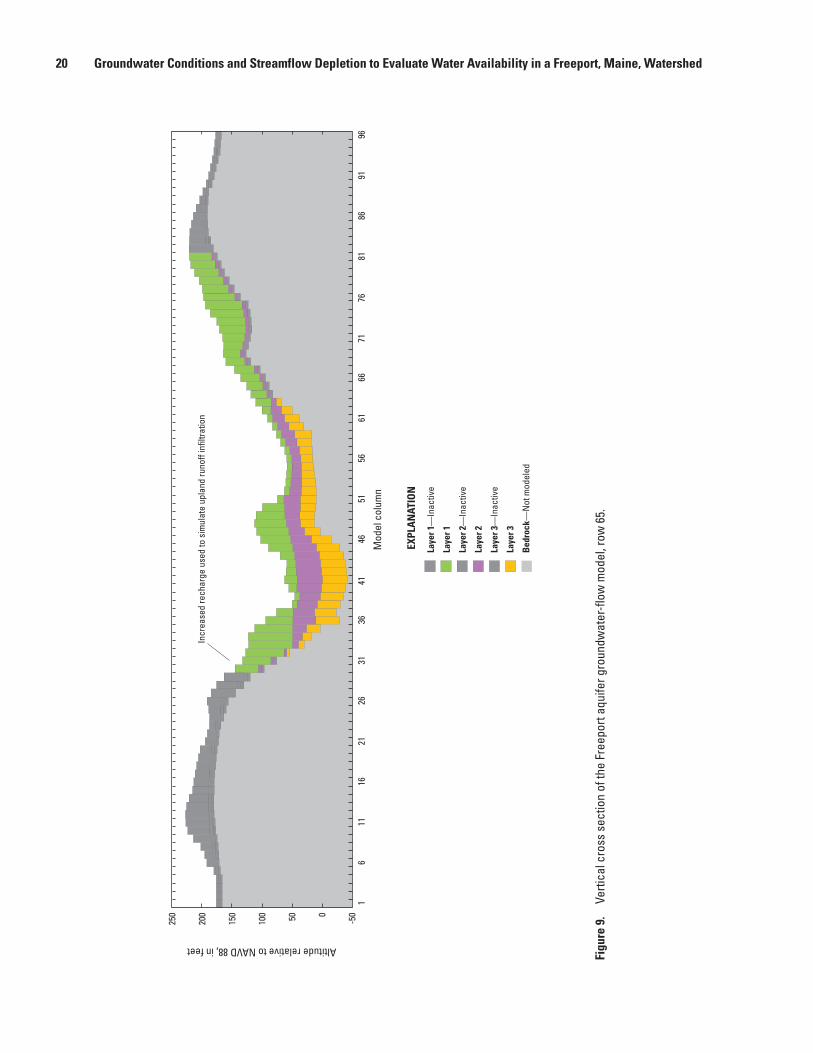
20 Groundwater Conditions and Streamflow Depletion to Evaluate Water Availability in a Freeport, Maine, Watershed
Figu
re 9
. Ve
rtica
l cro
ss s
ectio
n of
the
Free
port
aqui
fer g
roun
dwat
er-fl
ow m
odel
, row
65.
-50050100
150
200
250
Altitude relative to NAVD 88, in feet
16
1116
2126
3136
4146
5156
6166
7176
8186
9196
Mod
el c
olum
n
Incr
ease
d re
char
ge u
sed
to s
imul
ate
upla
nd ru
noff
infil
tratio
n
Laye
r 1—
Inac
tive
Laye
r 1
Laye
r 2—
Inac
tive
Laye
r 2
Laye
r 3—
Inac
tive
Laye
r 3
Bed
rock
—N
ot m
odel
ed
EXPL
AN
ATIO
N

Simulation of Groundwater Flow and Discharge to Streams 21
earlier. Zones of equal recharge were laid out based on the surficial geology and soil characteristics. Recharge rates were treated as model parameters during the optimization phase of model calibration and were adjusted within a range of reason-able values. The recharge rates used in the calibrated model are shown in figure 10. They range from 0.75 in/yr in the unweathered clay of the Presumpscot Formation to 25 in/yr in several areas of sandy soils, which is near the maxi-mum reasonable value calculated using Lyford and Cohen (1988). Recharge to the model was increased in the upper layer at the model edge to account for runoff entering from uplands to the west (fig. 9). To account for inflow to the model from upland runoff on the western edge of the model, an increased recharge rate of 50 in/yr was used in one thin zone running along a portion of the western edge of the model.
As discussed previously, the presence of the unsew-ered houses in the study area has the potential to effectively increase the recharge rate to the uppermost hydrogeologic layers by moving water from the bedrock aquifer to septic systems. If all 291 of the unsewered houses in the Freeport watersheds withdrew water from bedrock rather than the surficial units, the spatially-averaged recharge rate could be increased by 0.11 in/yr. This increase was considered generally negligible, and was grouped with the overall recharge rates.
Pumping was simulated for the AquaMaine water utility wells in layer 3 on the basis of long-term pumping records supplied by the water utility. The pumping wells are 250 ft apart (fig. 8). Average simulated withdrawals were 191 and 18 gallons per minute (gal/min). The well with the larger pumping rate is about 275 ft from Harvey Brook.
Hydraulic PropertiesHydraulic properties used in the model included stream-
bed hydraulic conductivity, horizontal hydraulic conductivity in the hydrogeologic units, anisotropy, and vertical hydrau-lic conductivity, which were distributed on the basis of the surficial geology and soils (Natural Resources Conservation Service, 2006) and refined during the calibration process. Horizontal hydraulic conductivity in the uppermost layer ranged from 0.56 to 13.6 ft/d (fig. 11A, table 5). Layer 2 was divided into two zones to coincide with the presence or absence of the Presumpscot Formation (fig. 11B, table 5). Horizontal hydraulic conductivity was 3.3 × 10⁻⁵ ft/d in zone 1, which corresponds to areas where the Presumpscot Formation was present and saturated, and 9.0 ft/d in zone 2, which repre-sents a mixture of till and the upper fractured and weathered zone of the Presumpscot Formation. Hydraulic conductivity of the lowest model layer ranged from 18.1 to 167 ft/d on the basis of the calibration process. All the hydraulic properties associated with the zones in layers 1 through 3 were treated as parameters during the optimization phase of the calibra-tion process (appendix 2 and table 6). Reasonable ranges were based on literature values and the results of past pumping test within the study area (table 1). The hydraulic conductivity of
the head-dependent flux boundaries on the north and south (fig. 5) was set to a relatively high value (246 ft/d) to facilitate the movement of water in and out of these boundaries. This value does fall within the reasonable range for the buried aqui-fer, as determined by pumping tests (table 1).
The calibrated vertical hydraulic conductivities (Kv) ranged from 3 × 10⁻⁶ ft/d in the Presumpscot Formation confin-ing unit to 16.4 ft/d in the buried valley sediments (fig. 12).
Simulated hydraulic conductivity values for the drains (Kdr) ranged from 0.017 to 5 ft/d (fig. 13), with the lowest val-ues being in the Merrill Brook watershed, which is underlain by shallow till and clayey soils. The streams with very low (0.017 and 0.02 ft/d) hydraulic conductivities are very small, and the 1.6 ft uniform streambed thickness used in the model is unreasonably large for these drain cells. Because the overall streambed leakance is inversely proportional to streambed thickness, the actual hydraulic conductivity of the streambed in these areas is probably substantially greater than what was used in the model. The upper range of Kdr values obtained is comparable to the Kdr values used in other Maine groundwater studies (table 1), and most values are within reasonable ranges for the hydraulic conductivities of the geologic materials in which they are situated. The model was somewhat sensitive to the drain conductance representing Harvey Brook and highly sensitive to the drain conductance representing Merrill Brook.
Model Calibration Using Parameter Estimation and Observations
Methods outlined in Hill and Tiedeman (2007) were followed during calibration using the UCODE_2005 software package (Poeter and others, 2008). These methods allow for the explicit accounting for uncertainty in both the water levels and streamflows used as calibration targets, documenting the model sensitivity to model variables, and sensitivity to data used in the model. During the prediction phase, these methods assist in documenting the uncertainty in the model predictions.
Statistics used to quantify the fit of the model to the observed values (the ability of the model to reproduce the observations) are used as the dependent variables in the parameter estimation, whereas the model parameters are treated as independent variables through a series of linear and nonlinear regression calculations. The optimization of the parameter values is conducted through an iterative process, during which the user uses the output of each iteration to determine which parameters can be estimated and whether trial-and-error changes to other parameters, or changes to the conceptual model, are needed. During the optimization process, the sensitivity of the model to each parameter value is determined for each optimization iteration, and only parameters that exceed a threshold sensitivity (and are not highly correlated with each other) are estimated. Hill and Tiedeman (2007) provide further details on the process of parameter estimation.

22 Groundwater Conditions and Streamflow Depletion to Evaluate Water Availability in a Freeport, Maine, Watershed
EXPLANATION
Recharge—In inches per year
0.750
5.04
7.1
10.75
24
25
50
96
30
90
40
20
10
60
50
80
70
130
140
100
110
120
148
0
10
30
90
20
60
80
40
50 701
Model row
Model column
Figure 10. Recharge rates applied to the numerical model of the Freeport aquifer study area.

Simulation of Groundwater Flow and Discharge to Streams 23A
. La
yer 1
B.
Laye
r 2C.
Lay
er 3
Act
ive
mod
el a
rea
0.56
0.69
1.6
10.7
13.6
0.00
0033
9.0
EXPL
AN
ATIO
NCa
libra
ted
hori
zont
al h
ydra
ulic
con
duct
ivity
(Kh)—
In fe
et p
er d
ay
Act
ive
mod
el a
rea
18.1
150
167
Act
ive
mod
el a
rea
Figu
re 1
1.
Calib
rate
d ho
rizon
tal h
ydra
ulic
con
duct
iviti
es (K
h) use
d in
the
Free
port
aqui
fer g
roun
dwat
er-fl
ow m
odel
.
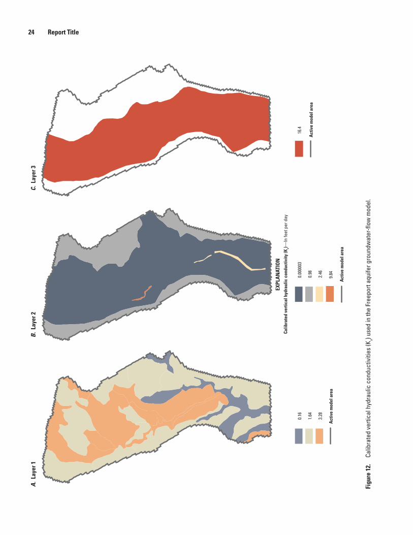
24 Report TitleA
. La
yer 1
B.
Laye
r 2C.
Lay
er 3
Act
ive
mod
el a
rea
0.16
1.64
3.28
16.4
Act
ive
mod
el a
rea
EXPL
AN
ATIO
NCa
libra
ted
vert
ical
hyd
raul
ic c
ondu
ctiv
ity (K
v)—In
feet
per
day
Act
ive
mod
el a
rea
0.00
0003
0.98
2.46
9.84
Figu
re 1
2.
Calib
rate
d ve
rtica
l hyd
raul
ic c
ondu
ctiv
ities
(Kv) u
sed
in th
e Fr
eepo
rt aq
uife
r gro
undw
ater
-flow
mod
el.

Simulation of Groundwater Flow and Discharge to Streams 25
EXPLANATION
Drain cell streambed hydraulic conductivity (Kdr) values—In feet per day
0.017
0.02
1.5
4.5
5
Active model area
96
30
90
40
20
10
60
50
80
70
130
140
100
110
120
148
0
10
30
90
20
60
80
40
50 701
Model row
Model column
Figure 13. Drain hydraulic conductivity values (Kdr) used in calibrated model.

26 Groundwater Conditions and Streamflow Depletion to Evaluate Water Availability in a Freeport, Maine, Watershed
ObservationsFor the Freeport aquifer numerical model, 54 head
observations and 5 flow observations were used (table 6). The head observations included water-level measurements from the wells, borings, and seismic line locations shown in figure 14. As stated earlier, the water-level measurements came from data collected over a long time span (1978–2009). For the wells with a long period of measurements, the value used for the observation is the mean of all the measurements. The distribution of head measurements in the model area was best in the central and northern parts of the model, but there were areas in the southern part of the model where there was no information at all on water levels. To stabilize the model, 11 estimated water-level observations were added in the uplands, primarily in the southern part of the model (fig. 14, table 6). These observations, measured in feet below land surface, were based on the average depth to water in all of the “till” wells in the statewide Maine USGS groundwater-level monitoring network. Overall, 30 of the head observations were in layer 1, 2 were in layer 2, and 22 were in layer 3.
The variance used to weight the observations for water levels in wells (table 6) included a combination of measurement, estimation, and altitude errors. Because of the long time period during which measurements were made (and several wells were measured once during that time span), the variance represented climatic differences among years of data collection and uncertainty about the water level itself. The uncertainty in the water levels with repeated measurements over time was based on the standard deviation about the mean of the total number of measurements. The uncertainty in the water-level measurements for wells or borings with
few, or only one, measurement, was set to ±3.28 ft (1 m). The uncertainty in water-level measurements for the seismic lines was also set at ±3.28 ft. The uncertainty in water-level measurements for the estimated water levels in till areas was ±6.5 ft (2 m). The errors from uncertainty in the altitude of the measuring point varied, depending on the source of the altitude data. Wells with precisely measured altitudes were assigned an uncertainty of ±0.5 to 1 ft. Wells, borings, and seismic lines with altitudes read from a topographic map were given an altitude error of ±6.4 ft, as were the water levels estimated in till (table 6).
The flow observations consisted of the sum of the drain cells in the subbasins of each of the five streamflow measurement sites (fig. 14). The streamflow observations were the 3-month average (May–July) of the statistical estimate of monthly flows based on the individual streamflow measurements, as described earlier. A rigorous analysis of the errors associated with these estimates was not performed, and a standard deviation of ±5 percent was used to calculate the variance. The streamflow observations also are presented in table 6. Additional details on the use of observations and weighting can be found in Hill and Tiedeman (2007).
Thirteen of the wells used for the observations had data for time periods when the pumping was not active but within the longer timeframe during which pumping has been in progress (since the early 1990s). Although these data were not used during the optimization phase, in the final stages of calibration, the drawdown in those wells (the difference between pumping and non-pumping heads) was compared to the drawdown predicted by the model and used to further refine the model.
Table 5. Hydrogeologic units and associated calibrated hydraulic conductivities.
[Kh, horizontal hydraulic conductivity; Kv, vertical hydraulic conductivity; ft/d, foot per day; Fm., formation; NA, not applicable]
Unit description LayerCalibrated Kh,
in ft/dCalibrated Kv,
in ft/d
Surficial sandy deposits above Presumpscot Fm. 1 13.6 3.28Surficial sandy deposits, eolian 1 13.6 3.28Till and weathered Presumpscot Fm., undivided 1 .69 1.64Weathered Presumpscot Fm. silt/clay 1 10.7 1.64Unweathered Presumpscot Fm. silt/clay 1 .56 .16Holocene alluvium and fine sand 1 1.6 3.28Till and weathered Presumpscot Fm., undivided 2 9.0 0.98Unweathered Presumpscot Fm. silt/clay 2 .00003 .000003Vertical flow zones in Presumpscot Fm. silt/clay
(2 separate zones)2 NA 9.84, 2.46
Fine sand, buried aquifer 3 18.1 16.4Coarse sand unit A 3 150 16.4Coarse sand unit B 3 167 16.4
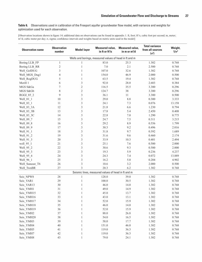
Simulation of Groundwater Flow and Discharge to Streams 27
Table 6. Observations used in calibration of the Freeport aquifer groundwater flow model, with variance and weights for optimization used for each observation.
[Observation locations shown in figure 14; additional data on observations can be found in appendix 1. ft, foot; ft3/s, cubic foot per second; m, meter; m3/d, cubic meter per day; σ, sigma; confidence intervals and weights based on metric units used in the model]
Observation nameObservation
numberModel layer
Measured value, in ft or ft3/s
Measured value, in m or m3/d
Total variance from all sources
(σ2)
Weight, 1/σ2
Wells and borings, measured values of head in ft and mBoring LLB_FP 1 1 83.0 25.3 1.302 0.768Boring LLB_RR 2 1 7.0 2.1 2.500 0.768Well_GolDUG 3 1 107.0 32.6 1.302 0.768Well_MGS_Dug1 4 1 154.0 46.9 2.000 0.500Well_RogDUG 5 1 63.5 19.4 1.302 0.768Merill 1 6 3 92.0 28.0 2.603 0.384MGS S&Ga 7 2 116.5 35.5 3.380 0.296MGS S&Gb 8 2 124.7 38 3.380 0.296RGGI_85_2 9 3 36.1 11 3.380 0.500Well_01_1 10 3 29.0 8.8 0.300 3.333Well_83_1 11 3 24.1 7.3 0.076 13.158Well_83_3A 12 3 21.8 6.6 1.230 0.794Well_83_3B 13 3 17.8 5.4 2.450 0.408Well_83_3C 14 3 22.8 7.0 1.290 0.775Well_89_7 15 3 24.7 7.5 0.311 3.215Well_89_8 16 3 29.2 8.9 0.556 1.799Well_89_9 17 3 30.3 9.2 0.496 2.016Well_91_1 18 3 31.8 9.7 0.592 1.689Well_91_2 19 3 31.6 9.6 0.460 2.174Well_91_3 20 3 33.9 10.3 0.401 2.494well_95_1 21 3 25.1 7.6 0.500 2.000Well_95_2 22 3 30.6 9.3 0.500 2.000Well_95_3 23 3 19.3 5.9 0.236 4.237Well_95_4 24 3 24.3 7.4 0.072 13.889Well_96_1 25 3 16.2 5.0 0.204 4.902Well_Suneast_T6 26 3 10.6 3.2 2.000 0.500Well_TwnBR 27 3 20.3 6.2 1.302 0.768
Seismic lines, measured values of head in ft and mSeis_NPW8 28 1 128.0 39.0 1.302 0.768Seis_YAR1 29 1 100.0 30.5 1.302 0.768Seis_YAR13 30 1 46.0 14.0 1.302 0.768Seis_YMH1 31 1 49.0 14.9 1.302 0.768Seis_YMH15 32 1 45.0 13.7 1.302 0.768Seis_YMH16 33 1 43.0 13.1 1.302 0.768Seis_YMH17 34 1 52.0 15.9 1.302 0.768Seis_YMH18 35 1 46.0 14.0 1.302 0.768Seis_YMH19 36 1 52.0 15.9 1.302 0.768Seis_YMH2 37 1 88.0 26.8 1.302 0.768Seis_YMH20 38 1 54.0 16.5 1.302 0.768Seis_YMH3 39 1 58.0 17.7 1.302 0.768Seis_YMH4 40 1 151.0 46.0 1.302 0.768Seis_YMH5 41 1 119.0 36.3 1.302 0.768Seis_YMH7 42 1 119.0 36.3 1.302 0.768Seis_YMH8 43 1 79.0 24.1 1.302 0.768
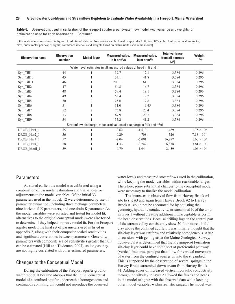
28 Groundwater Conditions and Streamflow Depletion to Evaluate Water Availability in a Freeport, Maine, Watershed
ParametersAs stated earlier, the model was calibrated using a
combination of parameter estimation and trial-and-error adjustments to the model variables. Of the initial 33 parameters used in the model, 12 were determined by use of parameter estimation, including three recharge parameters, nine horizontal K parameters, and one drain K parameter. As the model variables were adjusted and tested for model fit, alternatives to the original conceptual model were also tested to determine if they helped improve model fit. For the Freeport aquifer model, the final set of parameters used is listed in appendix 2, along with their composite scaled sensitivities and significant correlations between parameters. Generally, parameters with composite scaled sensitivities greater than 0.5 can be estimated (Hill and Tiedeman, 2007), as long as they are not highly correlated with other estimated parameters.
Changes to the Conceptual ModelDuring the calibration of the Freeport aquifer ground-
water model, it became obvious that the initial conceptual model of a confined aquifer underneath a homogeneous and continuous confining unit could not reproduce the observed
water levels and measured streamflows used in the calibration, while keeping the model variables within reasonable ranges. Therefore, some substantial changes to the conceptual model were necessary to finalize the model calibration.
The increases in observed flow from Harvey Brook #4 site to site #3 and again from Harvey Brook #2 to Harvey Brook #1 could not be accounted for by adjusting the geometry, hydraulic conductivity, or streambed K of the units in layer 1 without creating additional, unacceptable errors in the head observations. Because drilling logs in the central part of the stream valley consistently show 50 ft or more of silt/clay above the confined aquifer, it was initially thought that the silt/clay layer was uniform and relatively homogeneous. After discussions with geologists at the Maine Geological Survey, however, it was determined that the Presumpscot Formation silt/clay layer could have some sort of preferential pathway (vertical fractures, perhaps) that allow for vertical movement of water from the confined aquifer up into the streambed. This is supported by the observation of several springs in the Harvey Brook streambed downstream from Harvey Brook #1. Adding zones of increased vertical hydraulic conductivity through the silt/clay in layer 2 allowed the fluxes and heads in the model to agree with the observed data while keeping other model variables within realistic ranges. The model was
Table 6. Observations used in calibration of the Freeport aquifer groundwater flow model, with variance and weights for optimization used for each observation.—Continued
[Observation locations shown in figure 14; additional data on observations can be found in appendix 1. ft, foot; ft3/s, cubic foot per second; m, meter; m3/d, cubic meter per day; σ, sigma; confidence intervals and weights based on metric units used in the model]
Observation nameObservation
numberModel layer
Measured value, in ft or ft3/s
Measured value, in m or m3/d
Total variance from all sources
(σ2)
Weight, 1/σ2
Water level estimates in till, measured values of head in ft and mSyn_Till1 44 1 39.7 12.1 3.384 0.296Syn_Till10 45 1 137.1 41.8 3.384 0.296Syn_Till11 46 1 200.1 61 3.384 0.296Syn_Till2 47 1 54.8 16.7 3.384 0.296Syn_Till3 48 1 59.4 18.1 3.384 0.296Syn_Till4 49 1 56.4 17.2 3.384 0.296Syn_Till5 50 2 25.6 7.8 3.384 0.296Syn_Till6 51 1 31.0 9.45 3.384 0.296Syn_Till7 52 2 76.8 23.4 3.384 0.296Syn_Till8 53 1 67.9 20.7 3.384 0.296Syn_Till9 54 1 135.2 41.2 3.384 0.296
Streamflow discharge, measured values of discharge in ft3/s and m3/dDROB_Har1_1 55 1 -0.62 -1,513 1,489 1.75 × 10⁻⁴
DROB_Har2_1 56 1 -0.29 -708 326 7.98 × 10⁻⁴
DROB_Har3_1 57 1 -2.04 -5,001 16,277 1.60 × 10⁻⁵
DROB_Har4_1 58 1 -1.33 -3,242 6,838 3.81 × 10⁻⁵
DROB_Meril_1 59 1 -0.79 -1,944 2,459 1.06 × 10⁻⁴

Simulation of Groundwater Flow and Discharge to Streams 29
!!
!.
!.!.
!.
!.
!.!.!.!.!.!.
!.!.!.!.
!.
!.!.
!.
!.
!.
!.
!.
!.!.
!.
!.
!.
!.
!.
!.!.
!.
!.
!.
!.
!.
!.!.
!.!.
!.
!.
!.
!.
!.
!.
!.
!.
!.
!.
!.
!.
!.
!.
!.
!.
!.
!.
!.
!.
!.
!.
##
#
#
#
6
3
1
2
4
8
7
9
5
53
46
45
54
52
51
50
49
48
47
44
A1
A3
A3A2
A5
A8
A9
A4
A6
36
3233
3534
38
40
42
43
39
3137
41
26
28
30
29
17
10
20
Freeport
Pownal
Yarmouth
North Yarmouth
58
56
5955
Harve
y Broo
k
Merrill
Broo
k
Cou
sins
Riv
er
70°8'070°10'
43°52'
43°50'
!
!!.!.
!.
!.!.
!. !.!.
!.
!.
!.!.
!.
!.
# 21
22
1624
27
11
2325
1412
13
15
18
19
57
A10
A11
Areaof inset
0 500 FEET250
0 200 METERS100
0 1 20.5 KILOMETERS
0 10.5 MILEBase from U.S. Geological Survey digital data, 1:24,000Universal Transverse Mercator projection, Zone 19NCentral meridian -69°Shaded relief from U.S. Geological Survey National ElevationDataset 10-meter digital elevation modelNorth American Datum of 1983 (NAD 83)
295
EXPLANATION
Active model area boundary
Buried valley extent
# Streamflow site and identifier
Groundwater level points
!. Confined, wells and borings
!. Unconfined, wells and borings
!. Unconfined, spring
!. Unconfined, seismic
!. Unconfined, synthetic
! Pumping well
Figure 14. Groundwater level and streamflow measurement observations in the Freeport aquifer study area, Maine. Points labeled with an “A” were not included in the model. Additional information on labeled points is provided in table 6 and appendix 1.

30 Groundwater Conditions and Streamflow Depletion to Evaluate Water Availability in a Freeport, Maine, Watershed
not sensitive enough to the specific Kv values in these zones to estimate them, although the model was very sensitive to their existence. More detailed geologic mapping, streamflow data collection, or drilling could provide data that would lead to further modifications and improvements to the conceptual model of the flow system.
Model Fit to Observations
The overall model fit is assessed by evaluating observations and their simulated equivalents. The simulated water levels for the head observations at 27 wells and borings, 16 seismic lines, and 11 points of estimated water levels are graphed against the observed values in figure 15A. The match between the observed and simulated heads appears to be fairly good, especially in layer 3. The mean absolute difference between the observed and simulated heads is 6.7 ft in layer 1 and 3.7 ft in layer 3. These differences represent 4 percent of the total head change across the whole model. Weighted residuals represent the difference between observed and simulated, adjusted for the weight applied to each observation during calibration. Ideally, the weighted residuals would be randomly distributed, both in magnitude and location. A plot of the weighted residuals and unweighted simulated values (fig. 16) shows that there is a slightly greater range in negative residuals than positive residuals, but little in the way of pattern from low to high heads. Spatially (fig. 17), the weighted residuals in layer 3 do not have any particular pattern. Although the weighted residuals in layer 1 in the north-central part of the model are relatively large in magnitude, they are both positive and negative. The large weighted residuals correspond to an area that has a thin saturated zone above the confining layer, and small-scale heterogeneities not modeled in this layer can have large effects on the heads. Some of the difficulty in fitting the heads in layer 1 was not unexpected due to the limited dataset of shallow water levels. Furthermore, some points were collected in very steep terrain, where water levels can vary greatly over short distances. Small-scale adjustments to these areas in the absence of data to support them were not warranted during the model calibration process, although they could have improved the model fit.
Although the absolute differences between the simulated and observed water levels in the estimated till water-level points is quite high in many cases, the low weights of those points translate into relatively low weighted residuals. This should not be interpreted as indicating the model is “correct” in these areas, only that the model error in those areas is con-sidered less important to the goals of the model purpose than errors in other areas.
The head data in layer 3 were somewhat less difficult to fit for two reasons: (1) the target water level for many of these wells represents the average over a long-term record, and (2) most of the wells were clustered in one area around the pumping well. Differences between the observed and
model-calculated heads in layer 3 also may partially be a result of vertical gradients within the aquifer not being represented by the model, which only uses 1 layer to represent this aquifer. None of the observations in layer 3 are screened across the entire aquifer, which is quite heterogeneous vertically. The observation in layer 3 that was hardest to fit was boring 85-2. The uncertainty in this observation is quite high, because the water level was taken 25 years ago when the boring was drilled and no observation well was left in place. The aquifer is known to be heterogeneous in this area and the water level was measured during a time of drought.
Drawdown data from a 20-day pump test also were used to calibrate the model parameters in layer 3. Observed rebound in 13 wells when the pumping well was turned off for 2 days was compared to model-simulated steady-state differences in water levels at these wells with the pumping well active and turned off. Measured drawdown from pumping (the inverse of rebound) ranged from -1.1 to -32.5 ft (table 7). The simu-lated equivalent drawdowns ranged from -2.2 to -25.6 ft for the calibrated model. Most of the simulated drawdowns were somewhat greater than observed, which results from (1) the vertical averaging of the hydraulic conductivity field in the model, as compared to the lenses of higher-K sediments that some of these wells intersect, and (2) the simulation of steady-state conditions as compared to the relatively short-term drawdowns in the observations.
The observed and simulated streamflows in the reaches above the streamflow measurement sites shown in table 8 and figure 15B indicate that the fit of the streamflow data is very good, even though the weights assigned to the streamflow measurements were low. Because the streamflow observations represent discharge from hundreds of individual model cells, the exact spatial distribution of drain flows on a cell-by-cell basis is averaged out. The pattern generally fits well with observations in the field.
The calibration of the model using the UCODE_2005 software creates data that can be used to estimate the individual 95-percent confidence intervals on the streamflow simulated at the five streamflow measurement locations, shown in figure 18 (Hill and Tiedeman, 2007; Poeter and others, 2008). These calculated confidence intervals take into account all of the uncertainty in the estimated parameters and the uncertainty in the model variables set by trial and error, and the uncertainty in the observations, but they do not account for uncertainty in the possible variations in conceptual models that could have been used. The simulated streamflow for Harvey Brook #3 was the most uncertain, which reflects its influence by many factors, including recharge in several areas of the model, drain cell conductances, Kh in both layer 1 and layer 3, and Kv in layer 2. Because it is less influenced by discharge up through layer 2, the simulated streamflow for Harvey Brook #2 has the lowest amount of uncertainty calculated for this model.
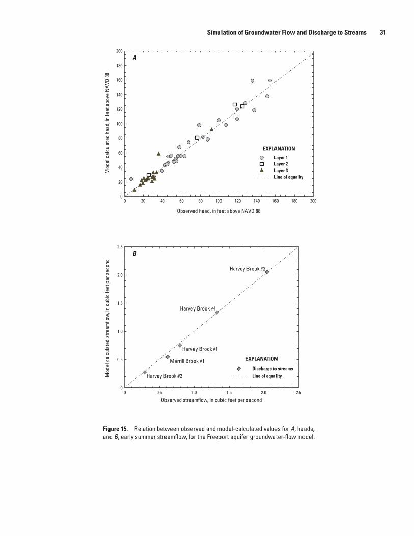
Simulation of Groundwater Flow and Discharge to Streams 31
Harvey Brook #1
Harvey Brook #2
Harvey Brook #3
Harvey Brook #4
Merrill Brook #1
B
A
Layer 1Layer 2Layer 3Line of equality
EXPLANATION
Discharge to streams
Line of equality
EXPLANATION
Mod
el c
alcu
late
d he
ad, i
n fe
et a
bove
NAV
D 88
Mod
el c
alcu
late
d st
ream
flow
, in
cubi
c fe
et p
er s
econ
d
Observed head, in feet above NAVD 88
Observed streamflow, in cubic feet per second
2.5
2.0
1.5
1.0
0.5
0
0
20
40
60
80
100
120
140
160
180
200
0 20 40 60 80 100 120 140 160 180 200
2.52.01.51.00.50
Figure 15. Relation between observed and model-calculated values for A, heads, and B, early summer streamflow, for the Freeport aquifer groundwater-flow model.

32 Groundwater Conditions and Streamflow Depletion to Evaluate Water Availability in a Freeport, Maine, Watershed
Simulated Groundwater Levels and Flow Under Steady-State Conditions
The simulated steady-state heads in model layers 1 and 3 are represented in figures 19 and 20, respectively. The layer 1 heads follow the terrain, with higher heads on the hills and valley edges, and lower heads in the stream valleys. Heads are highest in the upland hills along the northeast edge of the model, and decline to the west toward Harvey Brook. The representation of head in the Merrill Brook watershed follows the land surface contours quite well. Simulated groundwater flow is from areas of higher head to lower head, which in this case is from upland areas downhill toward the stream network. Simulated flow from the upper saturated zones in layer 1 through layer 2 and into layer 3 occurs where heads in layer 1 are higher than those in layer 3. This process occurs primarily along the western edge of the model and about halfway down the slope on the eastern edge of the model, where simulated recharge flows around the edge of the confining layer and into layer 3.
The modeled heads in layer 3 (fig. 20) are highest at the northern edge of the model and on the eastern and west-ern edges of the aquifer, where recharge enters from upland areas. The simulated pumping wells create a cone of depres-sion in the center of the model, and heads decline gradually from there toward the southern edge of the model. Simulated discharge upwards to the streams through the vertical conduc-tance zones in layer 2 creates a fairly flat hydraulic gradient in the southern half of the model in layer 3. Recharge to layer 3 is greatest where the heads are highest at the western edge of the model within a half mile of the pumping wells.
The distribution of simulated steady-state discharge of groundwater from drain cells in layer 1 is shown in figure 21. The spatial pattern of simulated discharge shows that the areas of greatest discharge in the Harvey Brook #4 watershed occur along the eastern tributary of Harvey Brook. Springs are known to occur in this area, which is adjacent to the eolian sand deposits overlying Presumpscot Formation silt and clay. The highest simulated stream discharge in the Harvey Brook #3 watershed area occurs along the main stem of Harvey Brook, which is consistent with field observations. The eastern tributary of the stream in that watershed has somewhat higher simulated streamflows than expected, however, which prob-ably is reflective of uncertainties in the distribution and thick-ness of the Presumpscot Formation in that area. Simulated stream discharge in the Harvey Brook #2 watershed areas is fairly constant along Harvey Brook. The cone of depression caused by the modeled pumping wells in layer 3 (fig. 20) creates an area of lower simulated discharge, but it is possible that streamflow may actually move from the stream down into the lower aquifer. Because the model used the drain package (which only allows for one-way water movement, from the aquifer to the drain cell), this possibility could not be evalu-ated with the model. Stream discharge along the segment of Harvey Brook in the Harvey Brook #4 watershed area is quite high, which is consistent with the field observations of springs in that area. The simulated discharge for most of the Merrill Brook watershed area is quite low, except in the westernmost tributary where it is slightly higher. No field data were avail-able to compare against this finding.
The construction and calibration of the numerical groundwater model of the Freeport aquifer area provided important insights into the flow of water within the groundwa-ter system and the interaction of the groundwater system with the streams. Prior to the current modeling exercise, the source of groundwater discharge to Harvey Brook was unknown, and the pathway of recharge to the confined aquifer was also unknown.
Model Sensitivity Analysis and Parameter Uncertainty
All the heads in layer 1 were sensitive to Merrill Brook streambed K, to recharge in the sandy units, and to the K of the sandy units. The areas north of the pumping wells were also sensitive to the K of poorly-drained clayey deposits (till and weathered Presumpscot Formation sediments/rock). The layer 1 heads south of the pumping well also were sensitive to recharge in the areas having thin deposits over bedrock. Layer 3 heads were most sensitive to the hydraulic conductivity zones in layer 3, and to recharge in the enhanced recharge area to the west and on the highest-altitude areas in the east-central part of the model, but not to the general head boundaries. This finding indicates that locally-derived recharge is much more important than surface water inflow from the north in feeding the Freeport aquifer. None of the
Wei
ghte
d re
sidu
als
on s
imul
ated
hea
d
-6
-4
-2
0
2
4
6
0 50 100 150 200 250
Unweighted simulated head, in feet
Figure 16. Weighted residuals and unweighted simulated values for heads in the Freeport aquifer groundwater-flow model.

Simulation of Groundwater Flow and Discharge to Streams 33
!
!!!!
!
!
!
# #
#
####
#
#
##
#
!
!
!
!
!
!
!
!
!
!
!
!
!
!
!
!
!
!
!
#
#
#
#
#
#
#
#
#
#
#
#
#
#
#
EXPLANATION
Active model area
Layer 3
Layers 1 and 2—Weighted residuals
# Less than -3.0
# -3.0 to -2.1
# -2.0 to -1.1
# -1.0 to 0
! 0.01 to 1.0
! 1.1 to 2.0
! 2.1 to 3.0
! Greater than 3.0
Layer 3—Weighted residuals
# Less than -3.0
# -3.0 to -2.1
# -2.0 to -1.1
# -1.0 to 0
! 0.01 to 1.0
! 1.1 to 2.0
! 2.1 to 3.0
! Greater than 3.0
96
30
90
40
20
10
60
50
80
70
130
140
100
110
120
148
0
10
30
90
20
60
80
40
50 701
Model row
Model column
Figure 17. Spatial distribution of weighted residuals across the domain of the Freeport aquifer groundwater-flow model.
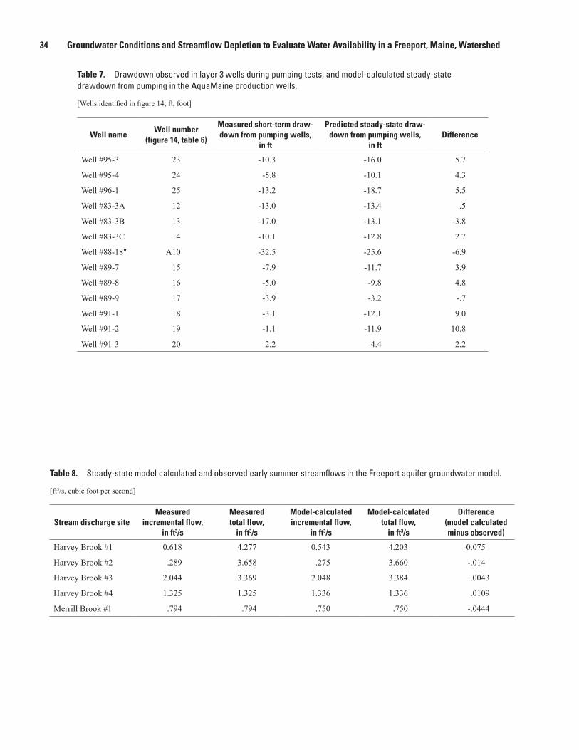
34 Groundwater Conditions and Streamflow Depletion to Evaluate Water Availability in a Freeport, Maine, Watershed
Table 7. Drawdown observed in layer 3 wells during pumping tests, and model-calculated steady-state drawdown from pumping in the AquaMaine production wells.
[Wells identified in figure 14; ft, foot]
Well nameWell number
(figure 14, table 6)
Measured short-term draw-down from pumping wells,
in ft
Predicted steady-state draw-down from pumping wells,
in ftDifference
Well #95-3 23 -10.3 -16.0 5.7
Well #95-4 24 -5.8 -10.1 4.3
Well #96-1 25 -13.2 -18.7 5.5
Well #83-3A 12 -13.0 -13.4 .5
Well #83-3B 13 -17.0 -13.1 -3.8
Well #83-3C 14 -10.1 -12.8 2.7
Well #88-18" A10 -32.5 -25.6 -6.9
Well #89-7 15 -7.9 -11.7 3.9
Well #89-8 16 -5.0 -9.8 4.8
Well #89-9 17 -3.9 -3.2 -.7
Well #91-1 18 -3.1 -12.1 9.0
Well #91-2 19 -1.1 -11.9 10.8
Well #91-3 20 -2.2 -4.4 2.2
Table 8. Steady-state model calculated and observed early summer streamflows in the Freeport aquifer groundwater model.
[ft3/s, cubic foot per second]
Stream discharge siteMeasured
incremental flow, in ft3/s
Measured total flow,
in ft3/s
Model-calculated incremental flow,
in ft3/s
Model-calculated total flow,
in ft3/s
Difference (model calculated minus observed)
Harvey Brook #1 0.618 4.277 0.543 4.203 -0.075
Harvey Brook #2 .289 3.658 .275 3.660 -.014
Harvey Brook #3 2.044 3.369 2.048 3.384 .0043
Harvey Brook #4 1.325 1.325 1.336 1.336 .0109
Merrill Brook #1 .794 .794 .750 .750 -.0444
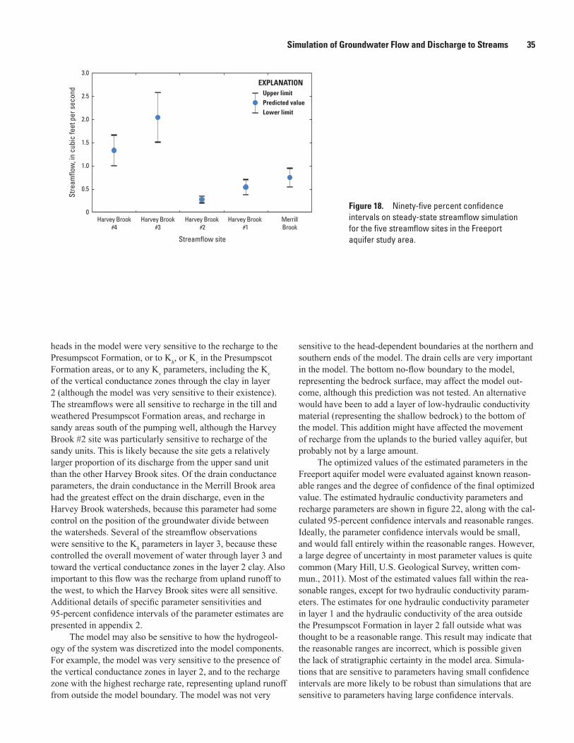
Simulation of Groundwater Flow and Discharge to Streams 35
heads in the model were very sensitive to the recharge to the Presumpscot Formation, or to Kh, or Kv in the Presumpscot Formation areas, or to any Kv parameters, including the Kv of the vertical conductance zones through the clay in layer 2 (although the model was very sensitive to their existence). The streamflows were all sensitive to recharge in the till and weathered Presumpscot Formation areas, and recharge in sandy areas south of the pumping well, although the Harvey Brook #2 site was particularly sensitive to recharge of the sandy units. This is likely because the site gets a relatively larger proportion of its discharge from the upper sand unit than the other Harvey Brook sites. Of the drain conductance parameters, the drain conductance in the Merrill Brook area had the greatest effect on the drain discharge, even in the Harvey Brook watersheds, because this parameter had some control on the position of the groundwater divide between the watersheds. Several of the streamflow observations were sensitive to the Kh parameters in layer 3, because these controlled the overall movement of water through layer 3 and toward the vertical conductance zones in the layer 2 clay. Also important to this flow was the recharge from upland runoff to the west, to which the Harvey Brook sites were all sensitive. Additional details of specific parameter sensitivities and 95-percent confidence intervals of the parameter estimates are presented in appendix 2.
The model may also be sensitive to how the hydrogeol-ogy of the system was discretized into the model components. For example, the model was very sensitive to the presence of the vertical conductance zones in layer 2, and to the recharge zone with the highest recharge rate, representing upland runoff from outside the model boundary. The model was not very
sensitive to the head-dependent boundaries at the northern and southern ends of the model. The drain cells are very important in the model. The bottom no-flow boundary to the model, representing the bedrock surface, may affect the model out-come, although this prediction was not tested. An alternative would have been to add a layer of low-hydraulic conductivity material (representing the shallow bedrock) to the bottom of the model. This addition might have affected the movement of recharge from the uplands to the buried valley aquifer, but probably not by a large amount.
The optimized values of the estimated parameters in the Freeport aquifer model were evaluated against known reason-able ranges and the degree of confidence of the final optimized value. The estimated hydraulic conductivity parameters and recharge parameters are shown in figure 22, along with the cal-culated 95-percent confidence intervals and reasonable ranges. Ideally, the parameter confidence intervals would be small, and would fall entirely within the reasonable ranges. However, a large degree of uncertainty in most parameter values is quite common (Mary Hill, U.S. Geological Survey, written com-mun., 2011). Most of the estimated values fall within the rea-sonable ranges, except for two hydraulic conductivity param-eters. The estimates for one hydraulic conductivity parameter in layer 1 and the hydraulic conductivity of the area outside the Presumpscot Formation in layer 2 fall outside what was thought to be a reasonable range. This result may indicate that the reasonable ranges are incorrect, which is possible given the lack of stratigraphic certainty in the model area. Simula-tions that are sensitive to parameters having small confidence intervals are more likely to be robust than simulations that are sensitive to parameters having large confidence intervals.
Upper limitPredicted valueLower limit
EXPLANATION
0
0.5
1.0
1.5
2.0
2.5
3.0St
ream
flow
, in
cubi
c fe
et p
er s
econ
d
Harvey Brook#4
Harvey Brook#3
Harvey Brook #2
Harvey Brook #1
MerrillBrook
Streamflow site
Figure 18. Ninety-five percent confidence intervals on steady-state streamflow simulation for the five streamflow sites in the Freeport aquifer study area.

36 Groundwater Conditions and Streamflow Depletion to Evaluate Water Availability in a Freeport, Maine, Watershed
!
!
!
!
!
!
!
!
!
!
!
!
!
!
!
!
!
!
!
!
!
!
!
!
!
!
!
!
!
!
!
##
#
#
#
Merrill BrookMerrill Brook
Harvey Brook #4Harvey Brook #4
Harvey Brook #3Harvey Brook #3
Harvey Brook #2Harvey Brook #2
Harvey Brook #1Harvey Brook #1
9080
70110
100
70
120100
90
80
110
40
50
60
20
30
30
60
50
40
8070
10
10130
140150
160170
180
190
60 50
30
30
3040
30
30
10
30
40
10
10
140
30
160
110120
100
40
170
10
8090
20
30
40
10
30
50
150
20
60
130120
20
10
5050
9090
9080
20
20
20
20
70
70
80
5060
6030
20
9080
70110
100
70
120100
90
80
110
40
50
60
20
30
30
60
50
40
8070
10
10130
140150
160170
180
190
60 50
30
30
3040
30
30
10
30
40
10
10
140
30
160
110120
100
40
170
10
8090
20
30
40
10
30
50
150
20
60
130120
20
10
5050
9090
9080
20
20
20
20
70
70
80
5060
6030
20
EXPLANATION
Active model areaLayer 1 head contour—Contour
interval 10 feet. Datum is NAVD 88
Layer 1 steady-state heads—Value
#0 Streamflow site and identifier! Layer 1 observation#
High: 193
Low: 0.4
96
30
90
40
20
10
60
50
80
70
130
140
100
110
120
148
0
10
30
90
20
60
80
40
50 701
Model row
Model column
Figure 19. Steady-state simulated groundwater levels in layer 1, Freeport aquifer model area. Contour interval is 10 feet.

Simulation of Groundwater Flow and Discharge to Streams 37
!
!!
!
!!!
! !!
!!
!!
!
!!
!
!
!
!.!.
5
75
70
65
60
10
80 85
55
100
95
5045
20
4035
90
85
15
3025
100105
20
15
80
5545
90
5
75
70
65
60
10
80 85
55
100
95
5045
20
4035
90
85
15
3025
105110115
100
20
60
15
80
5545
9590
!.
EXPLANATION
Active model area
Layer 3 head contour—Contour interval 5 feet. Datum isNAVD 88
Layer 3 steady-state heads—Value
Production well! Layer 3 observation
Layer 3 boundary
High: 117.2
Low: 3.2
96
30
90
40
20
10
60
50
80
70
130
140
100
110
120
148
0
10
30
90
20
60
80
40
50 701
Model row
Model column
Figure 20. Steady-state simulated groundwater levels in layer 3, Freeport aquifer model area. Contour interval is 10 feet.

38 Groundwater Conditions and Streamflow Depletion to Evaluate Water Availability in a Freeport, Maine, Watershed
Figure 21. Steady-state simulated streamflow (groundwater discharge) from drain cells and drain observation zones in the Freeport aquifer model area.
%%
Harvey Brook #4
Merrill Brook
Harvey Brook #3
Harvey Brook #2
Harvey Brook #1
Harvey Brook #4
Merrill Brook
Harvey Brook #3
Harvey Brook #2
Harvey Brook #1
Steady-state discharge from draincells—In cubic feet per day
Active model area
Drain observation zones
Pumping well%
EXPLANATION
< 50.00
50.01 to 150
150.1 to 300
300.1 to 475
475.1 to 675
675.1 to 900
900.1 to 1,300
1,301 to 1,670
1,671 to 2,250
2,251 to 3,500
3,501 to 10,000
10,010 to 18,500
96
30
90
40
20
10
60
50
80
70
130
140
100
110
120
148
0
10
30
90
20
60
80
40
50 701
Model row
Model column

Simulation of Groundwater Flow and Discharge to Streams 39
Figure 22. Parameter estimates, 95-percent confidence intervals, and reasonable ranges for A, hydraulic conductivity and B, recharge parameters for the Freeport aquifer groundwater-flow model.
A
B
0.01
0.10
1.00
10.00
100.00
1,000.00
0
5
10
15
20
25
30
35
40
Estimated hydraulic conductivity parameter
Hydr
aulic
con
duct
ivity
, in
feet
per
day
Rech
arge
, in
inch
es p
er y
ear
MaximumReasonable range
MinimumUpper limit
Optimal value
Lower limit
EXPLANATION
Estimated recharge parameter
KDR_
Mer
ill
HK_La
y1_A
HK_La
y1_B
HK_La
y1_C
HK_La
y1_C
D
HK_La
y1_D
HK_La
y2_T
L
HK_La
y3_S
a
HK_La
y3_K
2
HK_La
y3_K
3
RCH_T
ill
RCH_S
andy
N
RCH_S
andy
S

40 Groundwater Conditions and Streamflow Depletion to Evaluate Water Availability in a Freeport, Maine, Watershed
Limitations of the ModelThe Freeport aquifer groundwater-flow model pro-
vides a generalized simulation of the processes involved in groundwater recharge, flow, and discharge in the study area. The model is developed using observations of head and flow. Generally, models can simulate processes represented by observations used in the calibration, but are not well suited for the simulation of other processes. Therefore, this model is most appropriate for the simulation of flow and groundwater levels, but may not adequately simulate chemical transport. As with any numerical simulation of a natural system, the model incorporates simplifications and assumptions about the natural system that impose limitations in the use and interpretation of the model results. Some of the simplifications inherent in the model include a simplification of the surface-water system, a lack of incorporating the unsaturated zone, and the role of evapotranspiration in the water budget.
The stream network is simplified from reality, and the modeled streambed (drain) conductances incorporate very simplified representations of the width of each stream seg-ment. The discretization of the stream network also assumes a straight-line segment in each model cell, which may differ substantially from reality. The water-level altitudes in each model cell are interpolated from the topography in a way that may not represent each individual stream segment accu-rately. Finally, the conceptualization of the streamflow did not incorporate any potential losing reaches in Harvey Brook. Future modeling efforts that involve streamflow depletion and significant groundwater-surface water interactions may be improved using other packages in MODFLOW that allow for two-way movement of water between the aquifer and streams. Doing so would allow for losing reaches of streams as well as gaining reaches.
The boundaries were chosen for the model assuming that the surface-water divide coincides with the groundwater divide between watersheds. Limitations in the amount of field data—both in terms of the spatial and temporal distribution of measurements of groundwater levels and in terms of the data on the stratigraphy of the system—also translate into limitations in the model itself. More groundwater level data, particularly at the edges of the model, would help to constrain the boundary conditions and recharge. Additional stratigraphic data would have helped to make the movement of water more certain, particularly in the southern part of the model. There is some evidence of a certain amount of model error because although the model is sensitive to the recharge parameters, one of the recharge parameter estimates had to be constrained within the reasonable limits. This would not occur if the model construction perfectly matched physical reality. Similarly, some of the K parameters were estimated outside their reason-able ranges.
Finally, bedrock was considered to be a minor part of the overall water budget and was not modeled. However, adding a layer of shallow bedrock to the model may have reduced some of the model error.
Model-Calculated Water Budget for Harvey and Merrill Brooks and the Buried Freeport Aquifer
The simulated average annual water budget for three subareas of the Freeport aquifer study area (the Harvey Brook watershed in layer 1—Subarea 1; the modeled portion of the Merrill Brook watershed—Subarea 2; and the buried valley aquifer—Subarea 3) were calculated using the MODFLOW supplemental software ZONEBUDGET (Harbaugh, 1990). This software is used to calculate internal flows between dif-ferent zones of the model, which are summarized in table 9 along with the water budget of the entire model domain. Within this domain, recharge to surficial materials in layer 1 accounted for 91 percent of the total inflows (4.12 Mgal/d), with inflow from head dependent boundary cells account-ing for the remainder. Outflows from the model domain went to drain cells representing streams (90 percent), flux cells representing pumping wells (7 percent) and head-dependent boundary cells (2 percent). The model-calculated discrepancy between inflows and outflows was less than 0.001 percent. Of the total amount of recharge and other inflows entering the entire model domain, about 37 percent reaches the confined aquifer (Subarea 3). Simulated inflows and outflows beyond the boundaries of the Harvey and Merrill Brook watersheds (in the area around the Cousins River) are not included within Subareas 1 and 2.
The Harvey Brook watershed (Subarea 1), with its diverse geology and stream hydrology, has a more complex simulated water budget (table 9 and fig. 23) than the Merrill Brook watershed (Subarea 2). Subarea 1 receives more simulated recharge per unit land area than Subarea 2 because of its more permeable soils, and it also receives input in the form of upward groundwater seepage from layer 3, which is immediately discharged to the streams (fig. 23). This flow constitutes 27 percent of the total simulated inflows to the watershed, with the remainder consisting of recharge from precipitation (68 percent), horizontal subsurface flow from the Merrill Brook watershed (4 percent) and from other upland areas (1 percent). Simulated outflows from the Harvey Brook watershed are to streams (78 percent of the total) and downward infiltration to layers 2 and 3 (22 percent). The total simulated streamflow generated within the Harvey Brook watershed (2.7 Mgal/d) consists of shallow-generated streamflow from above the clay (1.8 Mgal/d) and the upward seepage from below the clay (0.9 Mgal/d) (table 9).
Of the two watersheds, Merrill Brook has the simpler simulated water budget, because of the shallow depth to bed-rock and widespread distribution of fine-grained materials. All simulated inflows to the Merrill Brook watershed (Subarea 2) come from recharge (table 9 and fig. 23); simulated outflows consist of discharge to streams (64 percent), infiltration to layer 3 (16 percent), horizontal subsurface flow to the Harvey Brook watershed (18 percent), and horizontal subsurface flow to other adjacent uplands (2 percent).
Subarea 3, the buried valley aquifer represented by layer 3, receives most of its input from downward seepage
Simulation of Groundwater Flow and Discharge to Streams 41
Table 9. Steady-state model calculated annual water budget for the Freeport aquifer groundwater-flow model and three subareas.
[Mgal/d, million gallons per day; Subarea 1 is Harvey Brook watershed; Subarea 2 is modeled portion of the Merrill Brook watershed; Subarea 3 is layer 3, buried valley deposits]
Hydrologic budget componentRate of flow, in Mgal/d
Entire model domain Subarea 1 Subarea 2 Subarea 3
Inflow
Recharge to surficial units 3.77 2.34 0.77Shallow subsurface flow from adjacent uplands .05Shallow subsurface flow from Merrill Brook watershed .13Flow up from layer 3 .93Infiltration down through layer 2 (till) 1.17From head-dependent boundaries 0.36 .36
Total inflow 4.12 3.45 .77 1.52Outflow
Groundwater discharge to streams 3.72 2.69 .49To head-dependent boundaries .10 .10Infiltration to layer 3 .77 .13Discharge upwards below streams 1.12Shallow subsurface flow to adjacent uplands .02Shallow subsurface flow to Harvey Brook watershed .13Water-supply withdrawals .30 .30
Total outflow 4.12 3.45 .76 1.52Budget error (inflow minus outflow) 0.000 0.001 0.000 0.000
through layer 2, and 98 percent of that flow occurs within what is simulated as the till zone of layer 2 (primarily within the Harvey Brook watershed). The remaining inflow to layer 3 is from the head-dependent boundary on the north end of the study area. Outflows from layer 3 are divided between the water-supply well withdrawals (20 percent), upward flow to streams in layer 1 (74 percent), and outflow from the head-dependent boundary on the south end of the model (7 percent).
The groundwater model was used to evaluate changes that could occur to the water budgets of the 3 subareas under four simulated climatic and pumping scenarios: (1) no pumping well withdrawals; (2) current (2009) pumping, but simulated drought conditions (equaling a 20-percent reduction in recharge); (3) current (2009) recharge, with a 50 percent increase in pumping well withdrawals for public supply; and (4) drought conditions and increased pumping combined. The water budgets for the model under these scenarios are pre-sented in figure 24 and table 10.
The effect of removing the pumping wells (0.3 Mgal/d) is primarily seen in the movement of water between layers 1 and 3 (tables 9 and 10). Hydraulic head in layer 3 is increased, the hydraulic gradient at the edges of the aquifer is reduced, and
infiltration from layer 1 to layer 3 is reduced by about 4 per-cent (from 1.17 to 1.12 Mgal/d). Beneath the Harvey Brook stream, however, the head in layer 3 is increased relative to the head in layer 1, and upward flow to the stream increases by about 23 percent (from 0.93 to 1.15 Mgal/d).
Simulated changes to the system from the drought sce-nario (a 20-percent decrease in total recharge, 0.76 Mgal/d, applied to each of the recharge zones) also affect the move-ment of water across the confining layer. Simulated head decreases in layer 3 as the infiltration downward from layer 1 to layer 3 in Harvey and Merrill Brook watersheds (Subareas 1 and 2) is reduced by 0.13 Mgal/d (13 and 17 per-cent, respectively), which is a nearly 15-percent reduction in downward recharge to Subarea 3 (table 10; fig. 24). This decrease however, is somewhat balanced by an increase in flow (0.03 Mgal/d) from the northern head-dependent boundary and a nearly 11-percent decrease in upward flow from layer 3 to the streams (0.13 Mgal/d). Simulated stream discharge from the whole model is reduced by 0.71 Mgal/d (19 percent), most of which comes from a reduction in the streamflow coming from recharge to layer 1.

42 Groundwater Conditions and Streamflow Depletion to Evaluate Water Availability in a Freeport, Maine, Watershed
A simulated 50-percent (0.15 Mgal/d) increase in pumping using the original recharge values resulted in slight changes to the hydrologic system and water budget. Modeled streamflow is reduced by 4 percent (0.14 Mgal/d), due primar-ily to decreased upward flow to Harvey Brook from layer 3 (about 0.11 Mgal/d, or 12 percent) as heads are reduced by the pumping increase.
Reducing the recharge combined with increasing pump-ing in the model resulted in the largest changes to the water budgets. The reduction in recharge (by 0.76 Mgal/d) and sub-sequent downward flow to layer 3 was balanced somewhat by an increase in flow of 0.04 Mgal/d from the north end of the model as head in layer 3 was lowered. Streamflow throughout the model was reduced by 0.85 Mgal/d (23 percent), and by 0.66 Mgal/d (24 percent) in the Harvey Brook watershed.
The simulation of the movement of water between different parts of the modeled hydrologic system illustrates the complexity of hydrologic systems in Maine. Although the base-case total water withdrawals from the system are only 7.2 percent of the entire water budget, those withdrawals do affect the hydrology of the system as a whole, and affect the
rates of flow in many areas of the model. Adding potential drought conditions to the simulations significantly altered the overall water budget, but it also altered the movement of water within the system, between layers and across the confining unit.
Evaluation of Streamflow Depletion in Harvey Brook
Direct instream withdrawals of water are simple to measure, and the effect on streamflows downstream of the withdrawal is readily understood. Groundwater withdrawals, on the other hand, can affect streamflows by varying amounts along a stream, and these affects can be difficult to measure. Surface-water or groundwater withdrawals may remove the same amount of water from the hydrologic system, but the effect of groundwater withdrawals on streamflow are distrib-uted over space and time. A reduction in streamflow result-ing from a groundwater withdrawal is known as streamflow
Inflows
Outflows
Flow
rate
, in
mill
ion
gallo
ns p
er d
ay
-4
-3
-2
-1
0
1
2
3
4
Suba
rea
1
Suba
rea
2
Suba
rea
3
EXPLANATION
Æ
Æ
Æ
Æ
Æ
Æ
Æ
Æ
Æ
Æ
Æ
Æ
Æ
To Harvey Brook watershed
To adjacent uplands
To wells
To head dependent boundary
Discharge up below streams
Infiltration to layer 3
To streams/drains
From Merrill Brook watershed
From uplands outside southwest divide
Up from layer 3
From head dependent boundary
From infiltration through till
From recharge
Inflow
Outflow
Figure 23. Steady-state simulated inflows and outflows for three subareas within the Freeport aquifer groundwater-flow system.

Evaluation of Streamflow Depletion in Harvey Brook 43
Flow rate, in million gallons per day
Subarea 1
Subarea 2
Subarea 3
Subarea 1
Subarea 2
Subarea 3
Subarea 1
Subarea 2
Subarea 3
Subarea 1
Subarea 2
Subarea 3
Subarea 1
Subarea 2
Subarea 3
Base
cas
eN
o pu
mpi
ngDe
crea
sed
rech
arge
Incr
ease
dpu
mpi
ngDe
crea
sed
rech
arge
and
incr
ease
d pu
mpi
ng
Inflo
ws
Outfl
ows
-4-3-2-101234
EXPL
AN
ATI
ON
ÆÆ ÆÆÆÆÆÆ Æ Æ Æ ÆÆ
To H
arve
y Br
ook
wat
ersh
ed
To a
djac
ent u
plan
ds
To w
ells
To h
ead
depe
nden
t bou
ndar
y
Disc
harg
e up
bel
ow s
tream
s
Infil
tratio
n to
laye
r 3
To s
tream
s/dr
ains
From
Mer
rill B
rook
wat
ersh
ed
From
upl
ands
out
side
sou
thw
est d
ivid
e
Up fr
om la
yer 3
From
hea
d de
pend
ent b
ound
ary
From
infil
tratio
n th
roug
h til
l
From
rech
arge
Inflo
w
Out
flow
Figu
re 2
4.
Sim
ulat
ed w
ater
bud
get c
ompo
nent
s un
der v
ario
us h
ydro
logi
c sc
enar
ios,
incl
udin
g no
pum
ping
, dec
reas
ed re
char
ge, a
nd in
crea
ses
in
pum
ping
for t
he F
reep
ort a
quife
r gro
undw
ater
-flow
mod
el.
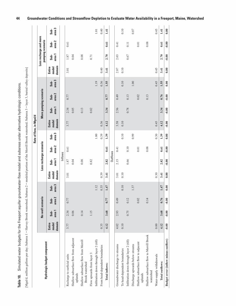
44 Groundwater Conditions and Streamflow Depletion to Evaluate Water Availability in a Freeport, Maine, WatershedTa
ble
10.
Sim
ulat
ed w
ater
bud
gets
for t
he F
reep
ort a
quife
r gro
undw
ater
-flow
mod
el a
nd s
ubar
eas
unde
r alte
rnat
ive
hydr
olog
ic c
ondi
tions
.
[Mga
l/d, m
illio
n ga
llons
per
day
; Sub
area
1 =
Har
vey
Bro
ok w
ater
shed
; Sub
area
2 =
mod
eled
por
tion
of th
e M
erril
l Bro
ok w
ater
shed
; Sub
area
3 =
laye
r 3, b
urie
d va
lley
depo
sits
]
Hyd
rolo
gic
budg
et c
ompo
nent
Rate
of f
low
, in
Mga
l/d
No
wel
l sce
nari
oLe
ss re
char
ge s
cena
rio
Mor
e pu
mpi
ng s
cena
rio
Less
rech
arge
and
mor
e
pum
ping
sce
nari
o
Entir
e m
odel
do
mai
n
Sub-
area
1Su
b-ar
ea 2
Sub-
area
3
Entir
e m
odel
do
mai
n
Sub-
area
1Su
b-ar
ea 2
Sub-
area
3
Entir
e m
odel
do
mai
n
Sub-
area
1Su
b-ar
ea 2
Sub-
area
3
Entir
e m
odel
do
mai
n
Sub-
area
1Su
b-ar
ea 2
Sub-
area
3
Inflo
ws
Rec
harg
e to
surfi
cial
uni
ts3.
772.
340.
773.
011.
870.
613.
772.
340.
773.
011.
870.
61
Shal
low
subs
urfa
ce fl
ow fr
om a
djac
ent
upla
nds
0.06
0.04
0.05
0.04
Shal
low
subs
urfa
ce fl
ow fr
om M
erril
l B
rook
wat
ersh
ed0.
140.
080.
130.
08
Flow
upw
ards
from
laye
r 31.
150.
820.
820.
71
Infil
tratio
n do
wn
thro
ugh
laye
r 2 (t
ill)
1.12
1.00
1.19
1.01
From
hea
d-de
pend
ent b
ound
arie
s0.
350.
350.
390.
390.
360.
360.
400.
40
Tota
l infl
ows:
4.12
3.68
0.77
1.47
3.41
2.82
0.61
1.39
4.12
3.34
0.77
1.55
3.41
2.70
0.61
1.41
Outfl
ows
Gro
undw
ater
dis
char
ge to
stre
ams
4.02
2.93
0.49
3.01
2.15
0.41
3.58
2.56
0.49
2.87
2.03
0.41
To h
ead-
depe
nden
t bou
ndar
ies
0.10
0.10
0.10
0.10
0.10
0.10
0.10
0.10
Infil
tratio
n do
wn
thro
ugh
laye
r 2 (t
ill)
0.75
0.12
0.66
0.10
0.78
0.13
0.67
0.11
Dis
char
ge u
pwar
ds b
elow
stre
ams
1.37
0.99
1.00
0.87
Shal
low
subs
urfa
ce fl
ow to
adj
acen
t up
land
s0.
020.
010.
020.
01
Shal
low
subs
urfa
ce fl
ow to
Mer
rill B
rook
w
ater
shed
0.14
0.08
0.13
0.08
Wat
er-s
uppl
y w
ithdr
awal
s0.
000.
300.
300.
450.
450.
450.
45
Tota
l out
flow
s:4.
123.
680.
761.
473.
412.
820.
611.
394.
123.
340.
761.
553.
412.
700.
611.
41
Bud
get e
rror
(infl
ow m
inus
out
flow
)-0
.00
-0.0
0-0
.00
0.00
0.00
-0.0
0-0
.00
0.00
-0.0
0-0
.00
-0.0
00.
000.
00-0
.00
-0.0
00.
00

Evaluation of Streamflow Depletion in Harvey Brook 45
depletion. Estimating this depletion at a particular location requires knowing how that withdrawal propagates through time and space across the river or stream. If one were to pick a stream location far enough downstream from the withdrawal, the total amount of overall depletion would equal the amount of withdrawal. If the withdrawal remained constant over the whole year, the effect of the withdrawal would be constant through the seasons. If the withdrawal varied with time, however, it would likely have variable effects on streamflow depletion that are difficult to determine.
Several methods exist for evaluating potential streamflow depletion, and two of them were applied in this study: the groundwater model and an analytical solution. The analytical solution was provided by use of the program STRMDEPL08. The following sections illustrate the effect of streamflow depletion on natural flows in the Freeport aquifer study area and the use and limitations of the two methods on evaluating streamflow depletion.
Calculation of Instream Flow Requirements for Harvey Brook
The instream flow requirements (seasonal aquatic base flows) for the State of Maine are designed to protect the aquatic health of riverine ecosystems, and vary with the seasons. The State regulations (Chapter 587 rules: Instream Flows and Lake and Pond Water Levels, part of the Maine Sustainable Water Use Program) define six different time periods during the year for which instream flows are calculated based on various median monthly flows. The most stringent of these requirements occurs during the summer (July 1 through September 15), when the instream flow requirement level is the August median flow.
Chapter 587 states that without site-specific flow data, the median monthly flows can be determined by using statewide flow equations developed by Dudley (2004), which best apply to watersheds larger than 10 mi2. Although these equations are not recommended for watersheds as small as those in the Freeport study area (Dudley, 2004), the State requirements indicate that these calculations can provide an interim estimate that may be refined with the collection of additional data. The seasonal instream flow requirements for the State, as defined in Chapter 587, are shown in figure 25 for Harvey and Merrill Brooks, along with the calculated median monthly flows from which these instream flows are based. The total amount of pumping from the water-supply wells in the Harvey Brook watershed is also shown.
Site-specific streamflow data for Harvey and Merrill Brooks were used to perform a record extension using the MOVE.1 method (described earlier), which is an acceptable alternative method of determining median monthly flows to use for the instream flow requirements (Ch. 587 rules). The median monthly flows estimated using the record extension are shown in figure 25 with the flows calculated using the statewide equations. The equation-based calculations and the
site-specific data agree closely for Merrill Brook, except in the winter (January–March), when the site-specific data indicate a lower natural median monthly flow than the statewide equa-tions predict (fig. 25A). The statewide equations did not per-form as well for Harvey Brook (fig. 25B), because of the large aquifer and more complex hydrologic system. The equations over-predict the natural flows for December through April, and predict a natural flow that is almost double what site-specific data would indicate for the April high-flow period. The state-wide equations predict the summer low-flow period fairly well for both streams, although the equations indicate a somewhat greater natural median flow in August and September than what was measured.
Because the statewide equations (Dudley, 2004) are predictions based on a statistical analysis of many other watersheds, the PRESS statistic can be used to calculate prediction intervals for each month as well as the individual monthly predicted value (Riggs, 1968). The prediction intervals indicate the level of certainty surrounding the individual monthly predicted value. For the Harvey Brook watershed, the 90-percent prediction intervals were calculated for each median monthly flow (fig. 26). The flows bounded by the prediction interval would be expected to contain the actual (measured) flow for a given stream 90 percent of the time. The measured flows for Harvey Brook fall well within the 90-percent prediction intervals for the months of May through November. The flows from December to February are at the lower edge of the 90-percent interval, and the measured flows for March and April are well below what was predicted, as well as what would be allowed for the maintenance of instream flows if site-specific data were not collected.
There is a clear benefit to using site-specific data against which to evaluate withdrawals and streamflow requirements, as it avoids potentially under- or over-estimating the natural instream flows. Because the goal of the State requirement is to protect natural flows but allow pumping if possible, under-standing the site-specific hydrologic regime would be very helpful in evaluating whether any particular flow was above or below the threshold.
Streamflow Depletion Estimates Based on STRMDEPL08
The analytical model STRMDEPL08 (Reeves, 2008) also was used to analyze streamflow depletion in Harvey Brook. STRMDEPL08’s analytical solutions assume that aquifers are homogeneous, isotropic, and infinite; because these conditions were not met for the Freeport aquifer, results are generalizations only. However, the results can be informative in determining what additional steps may be necessary to proceed with studying a particular situation. The usefulness of the analysis is limited by the degree to which the hydrology of the situation under analysis is understood and how well it fits the assumptions. The Freeport aquifer was modeled as a leaky aquifer underlying an aquitard, where the stream partially

46 Groundwater Conditions and Streamflow Depletion to Evaluate Water Availability in a Freeport, Maine, Watershed
BCubi
c fe
et p
er s
econ
d
0
5
10
15
20
25
Jan. Feb. Mar. Apr. May June July Aug. Sept. Oct. Nov. Dec.
Instream flow requirementsPumpingDudley method median flowsMOVE.1 median flows
EXPLANATION
Month
A
0
5
10
15
20
25
Instream flow requirements
Dudley method median flows
MOVE.1 median flows
EXPLANATION
Figure 25. Monthly median flow estimates, pumping, and instream flow requirements for A, Merrill Brook, and B, Harvey Brook, Freeport, Maine.
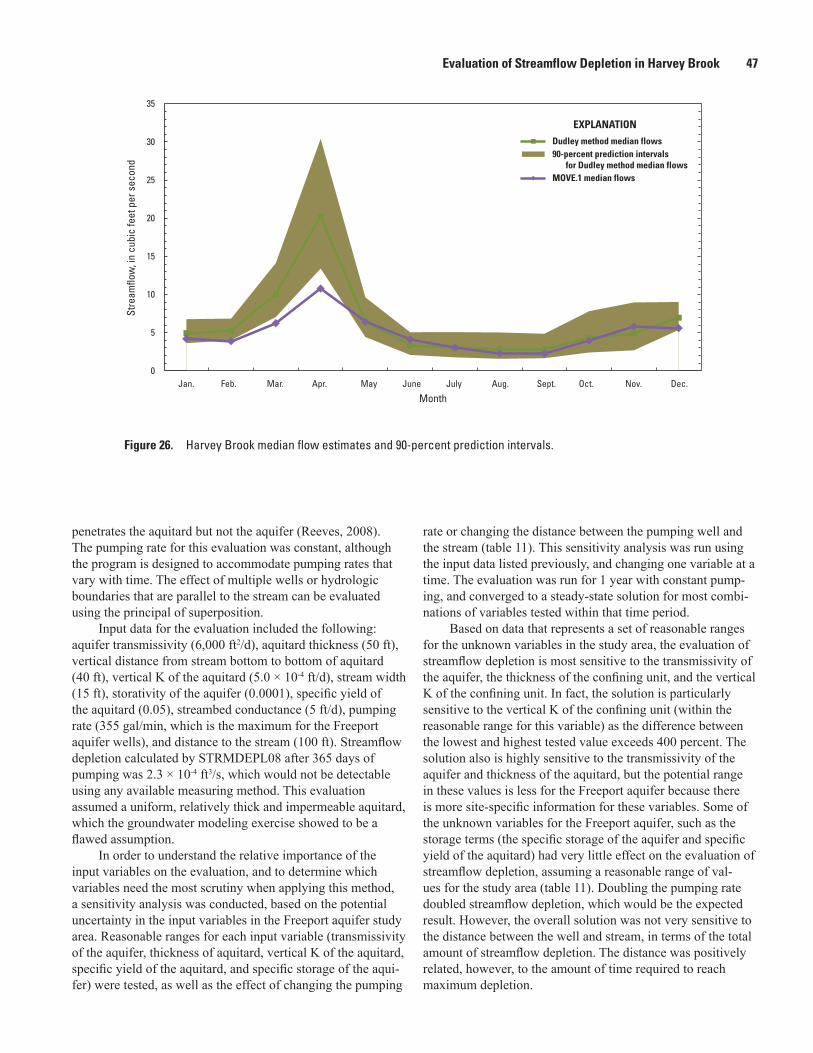
Evaluation of Streamflow Depletion in Harvey Brook 47
penetrates the aquitard but not the aquifer (Reeves, 2008). The pumping rate for this evaluation was constant, although the program is designed to accommodate pumping rates that vary with time. The effect of multiple wells or hydrologic boundaries that are parallel to the stream can be evaluated using the principal of superposition.
Input data for the evaluation included the following: aquifer transmissivity (6,000 ft2/d), aquitard thickness (50 ft), vertical distance from stream bottom to bottom of aquitard (40 ft), vertical K of the aquitard (5.0 × 10⁻⁴ ft/d), stream width (15 ft), storativity of the aquifer (0.0001), specific yield of the aquitard (0.05), streambed conductance (5 ft/d), pumping rate (355 gal/min, which is the maximum for the Freeport aquifer wells), and distance to the stream (100 ft). Streamflow depletion calculated by STRMDEPL08 after 365 days of pumping was 2.3 × 10⁻⁴ ft3/s, which would not be detectable using any available measuring method. This evaluation assumed a uniform, relatively thick and impermeable aquitard, which the groundwater modeling exercise showed to be a flawed assumption.
In order to understand the relative importance of the input variables on the evaluation, and to determine which variables need the most scrutiny when applying this method, a sensitivity analysis was conducted, based on the potential uncertainty in the input variables in the Freeport aquifer study area. Reasonable ranges for each input variable (transmissivity of the aquifer, thickness of aquitard, vertical K of the aquitard, specific yield of the aquitard, and specific storage of the aqui-fer) were tested, as well as the effect of changing the pumping
rate or changing the distance between the pumping well and the stream (table 11). This sensitivity analysis was run using the input data listed previously, and changing one variable at a time. The evaluation was run for 1 year with constant pump-ing, and converged to a steady-state solution for most combi-nations of variables tested within that time period.
Based on data that represents a set of reasonable ranges for the unknown variables in the study area, the evaluation of streamflow depletion is most sensitive to the transmissivity of the aquifer, the thickness of the confining unit, and the vertical K of the confining unit. In fact, the solution is particularly sensitive to the vertical K of the confining unit (within the reasonable range for this variable) as the difference between the lowest and highest tested value exceeds 400 percent. The solution also is highly sensitive to the transmissivity of the aquifer and thickness of the aquitard, but the potential range in these values is less for the Freeport aquifer because there is more site-specific information for these variables. Some of the unknown variables for the Freeport aquifer, such as the storage terms (the specific storage of the aquifer and specific yield of the aquitard) had very little effect on the evaluation of streamflow depletion, assuming a reasonable range of val-ues for the study area (table 11). Doubling the pumping rate doubled streamflow depletion, which would be the expected result. However, the overall solution was not very sensitive to the distance between the well and stream, in terms of the total amount of streamflow depletion. The distance was positively related, however, to the amount of time required to reach maximum depletion.
Jan. Feb. Mar. Apr. May June July Aug. Sept. Oct. Nov. Dec.
Month
0
5
10
15
20
25
30
35
Stre
amflo
w, i
n cu
bic
feet
per
sec
ond
90-percent prediction intervalsfor Dudley method median flows
Dudley method median flows
MOVE.1 median flows
EXPLANATION
Figure 26. Harvey Brook median flow estimates and 90-percent prediction intervals.

48 Groundwater Conditions and Streamflow Depletion to Evaluate Water Availability in a Freeport, Maine, Watershed
These results illustrate that conducting a cursory evalua-tion of streamflow depletion using available information may result in a very wide range in results, depending on how well the hydraulic conductivity variables and aquifer geometry are known. Without using a range in the possible variables, it would be impossible to use an analytical solution to give an estimate of streamflow depletion at a given location that can be known with any degree of certainty. However, the tool can be used to help understand which variables are most important to refine in order to increase the certainty in the estimate. In this case, the analysis shows that the vertical conductivity of the confining unit is crucial. This also was confirmed during the calibration of the groundwater-flow model.
Simulation of Streamflow Depletion Based on the Steady-State Groundwater-Flow Model
The groundwater-flow model was used as an alternate, more robust method to evaluate streamflow depletion. Current
streamflow depletion was calculated as the difference between streamflow (discharge to drain cells) with no pumping (no simulated withdrawals from the calibrated model) and stream-flow with pumping (the base-case calibrated model) (table 12). Streamflow depletion was 0.38 ft3/s, or about 8.5 percent of the base flow in Harvey Brook, and 0.01 ft3/s in Merrill Brook.
Streamflow depletion in the uppermost subbasin of the Harvey Brook watershed (Harvey Brook site #4) is negligible; most of the depletion occurs within the lower three stream segments, increasing from 0.23 ft3/s at Harvey Brook site #3 to 0.38 ft3/s at Harvey Brook site #1. Most of the change in streamflow occurs above Harvey Brook site #3, and about half that amount occurs between Harvey Brook sites #1 and #2. Only a small amount of the total depletion occurs in the upper reaches (recharge areas) of the subbasins (fig. 27). Some of the effect on pumping occurs outside the measured subbasins, and downstream of the measured sites.
The 95-percent confidence intervals on streamflow depletion estimates were calculated using UCODE_2005 (Poeter and others, 2008), and are shown in figure 28.
Table 11. Sensitivity analysis of STRMDEPL08 streamflow depletion evaluations for the Freeport aquifer, based on reasonable ranges for unknown variables.
[ft3/d, cubic foot per day; max, maximum; min, minimum; ft2, square foot per day; d, day; K, hydraulic conductivity; gal/min, gallon per minute]
VariableReasonable range tested
Streamflow depletion after 1 year of pumping,
in ft3/dPercent difference
(max-min/min)Low High Low result High result
Transmissivity of the aquifer, in ft2/d 4,000 13,000 2.83 × 10⁻⁴ 1.57 × 10⁻⁴ 45Specific storage of the aquifer .00001 .001 2.28 × 10⁻⁴ 2.19 × 10⁻⁴ 4Thickness of the aquitard, in ft 30 80 3.63 × 10⁻⁴ 1.66 × 10⁻⁴ 54Vertical K of the aquitard, in ft/d .00028 .005 2.31 × 10⁻⁴ 1.22 × 10⁻³ 428Specific yield of the aquitard .01 .1 2.48 × 10⁻⁴ 2.29 × 10⁻⁴ 8Distance from well to stream, in ft 25 1,000 2.32 × 10⁻⁴ 2.25 × 10⁻⁴ 3Pumping rate, in gal/min 178 355 1.18 × 10⁻⁴ 2.32 × 10⁻⁴ 97
Table 12. Model-calculated streamflow depletion at each streamflow measurement site.
[ft3/s, cubic foot per second]
Streamflow siteModel-calculated total steady-state streamflow with pumping,
in ft3/s
Predicted total steady-state streamflow without pumping,
in ft3/s
Incremental streamflow depletion (difference),
in ft3/s
Cumulative streamflow depletion,
in ft3/s
Harvey Brook #4 1.34 1.34 0.00 0.00Harvey Brook #3 3.39 3.62 .23 .23Harvey Brook #2 3.67 3.92 .02 .25Harvey Brook #1 4.21 4.59 .13 .38Merrill Brook .75 .76 .01 .01
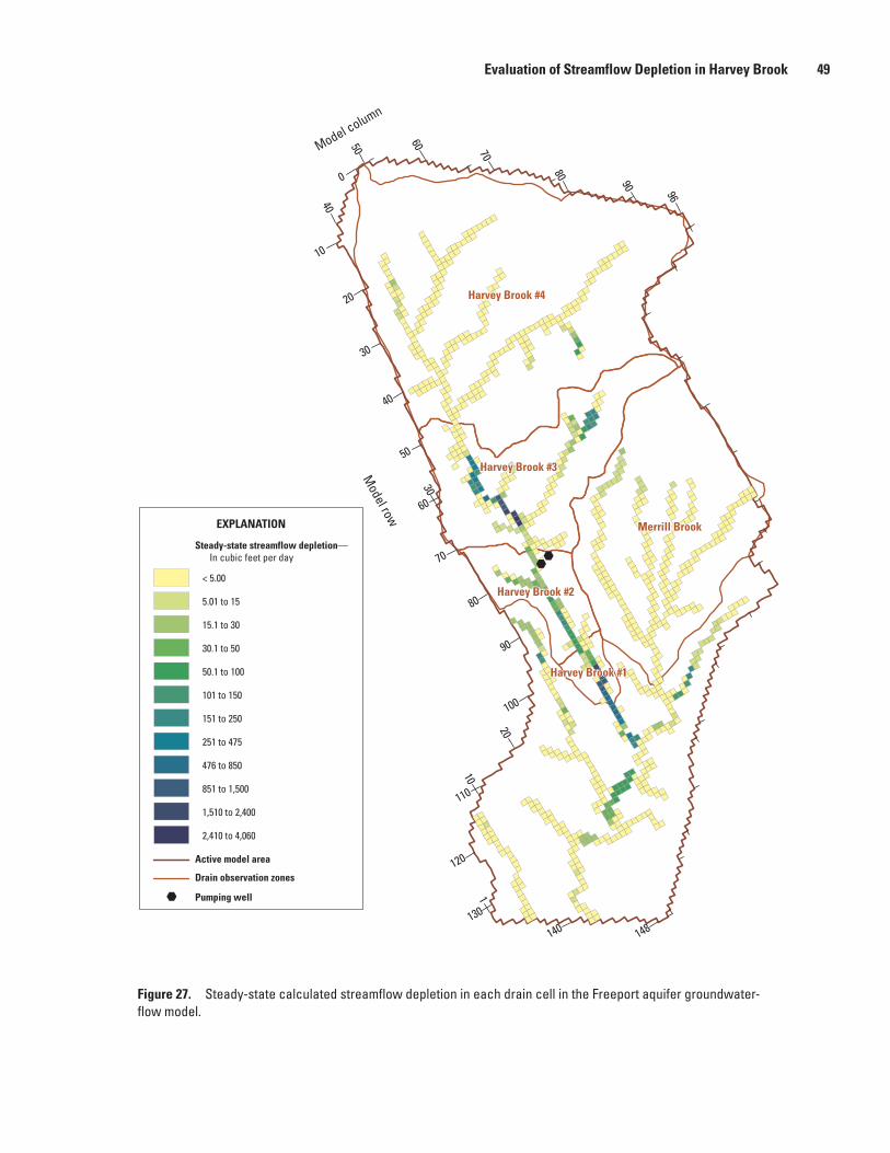
Evaluation of Streamflow Depletion in Harvey Brook 49
Figure 27. Steady-state calculated streamflow depletion in each drain cell in the Freeport aquifer groundwater- flow model.
%%
Harvey Brook #4
Merrill Brook
Harvey Brook #3
Harvey Brook #2
Harvey Brook #1
Harvey Brook #4
Merrill Brook
Harvey Brook #3
Harvey Brook #2
Harvey Brook #1
EXPLANATION
Drain observation zones
Steady-state streamflow depletion—In cubic feet per day
< 5.00
5.01 to 15
15.1 to 30
30.1 to 50
50.1 to 100
101 to 150
151 to 250
251 to 475
476 to 850
851 to 1,500
1,510 to 2,400
2,410 to 4,060
Active model area
% Pumping well
96
30
90
40
20
10
60
50
80
70
130
140
100
110
120
148
0
10
30
90
20
60
80
40
50 701
Model row
Model column

50 Groundwater Conditions and Streamflow Depletion to Evaluate Water Availability in a Freeport, Maine, Watershed
These confidence intervals take all the expressly identified uncertainty in parameter values and observations into account (as previously discussed). For the depletion simulations in the two stream segments with the most depletion (Harvey Brook #3 and Harvey Brook #1), most of the range in the confidence intervals fall above the line of zero streamflow depletion. The widest confidence band, for the segment above Harvey Brook site #3, reflects the combined inflows to that segment from layers 1 and 3, and the combined uncertainty from many different parameters that relate to groundwater flow in that area. The narrowest confidence band is for the segment above Harvey Brook site #2, which reflects the dominance of layer 1 (and fewer parameters) in the streamflow generation in that segment.
The 95-percent confidence intervals for streamflows and streamflow depletion also can be used to help illustrate the projected streamflows in Harvey and Merrill Brooks under the different pumping and recharge scenarios discussed earlier. The steady-state simulated drain discharge (streamflow) projected for Harvey and Merrill Brooks is compared to the prediction of streamflow with no pumping, with increased pumping (by 50 percent), with a 20 percent reduction in recharge, and increased pumping combined with decreased recharge (fig. 29, table 13). The streamflow in Harvey Brook is projected to decrease from 4.21 to 3.18 ft3/s (about a 25 percent drop) if pumping were increased and recharge was somewhat lower than it is currently. Of that reduction, some is from increased streamflow depletion, but most of the change is caused by the reduction in recharge. The change in streamflow for Merrill Brook would be less pronounced under that scenario, because it is not affected by pumping (although it is affected by recharge as much as Harvey Brook). Overall, Harvey Brook streamflow at site #1 could decrease to 3.37 ft3/s under a drought, without any change in pumping.
Comparison of Methods Used to Evaluate Streamflow Depletion
The estimates of streamflow depletion from the ground-water-flow model and from the STRMDEPL08 runs are substantially different. The STRMDEPL08 runs, which were done using the best available data from the pump tests, drilling records, and consultant reports from the water utility, indicated that negligible amounts of streamflow depletion are caused by the pumping of the water-supply wells in the buried aquifer, although the result is very sensitive to the chosen values for the hydraulic conductivity variables in the analysis. Con-versely, the calibrated groundwater-flow model indicated that streamflow depletion in Harvey Brook is about 8.5 percent of the natural, unaltered flow. Even when the 95-percent con-fidence intervals are taken into consideration, it is clear that at least some measurable amount of streamflow depletion likely occurs, and it may be larger than indicated here. Using the STRMDEPL08 tool to evaluate the streamflow depletion with an incomplete understanding of the hydrologic system gave results that seem unlikely to reflect the actual streamflow depletion situation in the Freeport aquifer study area.
Comparison of Streamflow Depletion Estimates to Instream Flow Requirements
To conduct a comparison of the instream flow requirements to the site-specific data (including the modeled streamflow depletion) in Harvey Brook, the summer time period (June 1 to August 31) was chosen. As described earlier, measurements were made to estimate the median monthly flows using the MOVE.1 regression technique. However, with the withdrawals being active at the time, the measurements do not represent the natural flow, but rather, the flows altered by streamflow depletion. Therefore, in order to use site-specific
Figure 28. Ninety-five-percent confidence intervals for simulated streamflow depletion caused by pumping for the Harvey and Merrill Brook sites.
Stre
amflo
w d
eple
tion,
in c
ubic
feet
per
sec
ond
-0.30
-0.20
-0.10
0.00
0.10
0.20
0.30
0.40
0.50
0.60
0.70
Upper limitPredicted valueLower limit
EXPLANATION
Harvey Brook #4
Harvey Brook #3
Harvey Brook #2
Harvey Brook #1
Merrill Brook
Streamflow site

Evaluation of Streamflow Depletion in Harvey Brook 51
Figure 29. Steady-state streamflow projections from the groundwater model for Harvey and Merrill Brooks for pumping and recharge scenarios, showing the 95-percent confidence intervals.
Stre
amflo
w, i
n cu
bic
feet
per
sec
ond
0
1
2
3
4
5
6
Model calibrated
No pumping
Increased pumping
Decreased recharge
Decreased recharge and
increased pumping
Harvey Brook upper 95-percent confidence limit
Harvey Brook #1
Harvey Brook lower 95-percent confidence limit
Merrill Brook upper 95-percent confidence limit
Merrill Brook
Merrill Brook lower 95-percent confidence limit
EXPLANATION
Streamflow site
Table 13. Model-calculated streamflow and streamflow depletion in Harvey Brook and Merrill Brook under various pumping and recharge scenarios.
[ft3/s, cubic foot per second]
Scenario Merrill Brook Harvey Brook #1
Total amount of model-calculated streamflow (in ft3/s)
Model-calculated steady-state with existing pumping 0.75 4.21Predicted steady-state without pumping .76 4.59Predicted with pumping increased by 50 percent .75 4.01Predicted with 20 percent less recharge .63 3.37Predicted with increased pumping and 20 percent less recharge .63 3.18
Incremental streamflow depletion1
Model-calculated steady-state with existing pumping .01 .38Predicted with pumping increased by 50 percent .01 .58Predicted with 20 percent less recharge .13 1.22Predicted with increased pumping and 20 percent less recharge .13 1.41
1Difference between no pumping and the other scenarios (in ft3/s).

52 Groundwater Conditions and Streamflow Depletion to Evaluate Water Availability in a Freeport, Maine, Watershed
measurements to accurately determine monthly flow amounts, there must be an independent evaluation of streamflow depletion that can be used to adjust the measured flows. (At minimum, the total amount of the withdrawal could be added to the measured flows for a conservative evaluation of flow.) The groundwater-flow model of the Freeport aquifer has shown that for the watersheds in the Freeport study area, the streamflow depletion is about 0.38 ft3/s for Harvey Brook, but essentially zero for Merrill Brook. Figure 30 illustrates the instream flow requirements for Harvey Brook at site #1 and the median monthly flows for June, July, and August as determined by Dudley’s (2004) statewide equations. The graph also shows the median monthly flows as determined by the site-specific measurements (the MOVE.1 median flows), and what would be the “natural” flows if pumping were not occurring in the aquifer. The “natural” median monthly flow for August agrees closely with what is predicted by the statewide equations, although the June and July flows are underestimated using those equations (fig. 30). As the instream flow requirement is set by the August flows, it appears that the measured flows in Harvey Brook are less than what would be allowed, and would be even lower if pumping were increased (fig. 30). From table 13, the difference between the steady-state “natural” flows (without pumping, 4.59 ft3/s) and the flows with pumping for Harvey Brook at site #1 if a drought occurred (a 20-percent reduction in recharge, 3.37 ft3/s) is 1.22 ft3/s, and the predicted amount of depletion with increased pumping and a drought together is 1.41 ft3/s.
Applying this amount of modeled depletion to the measured median monthly flows indicates that the resulting streamflow could fall well below what the 90-percent confidence limits for the statewide equation would predict (fig. 30).
Suggestions for Improving Methods of Study for Water Availability
Using the Freeport aquifer study as a pilot for future studies of water availability in “watersheds at risk” in Maine provides an opportunity to evaluate the procedures used herein to study water availability. Improvements to numerical groundwater modeling to reduce the uncertainty in the results could include (1) conducting a synoptic groundwater-level survey in which groundwater levels are measured in as many wells as possible during a short time frame (one week or less); (2) use a different package in MODFLOW, such as the streamflow-routing package (SRF) that allows flow into and out of cells, instead of the drain (DRN) package which only allows for gaining stream reaches; (3) include a layer of shallow bedrock underneath the unconsolidated aquifer materials, to decrease numeric instability and allow for a small amount of groundwater exchange between the bedrock and unconsolidated materials; and (4) divide the principal aquifer into additional vertical layers, particularly if there is evidence of vertical layering within the sediments.
Figure 30. Summer streamflows, pumping, instream flow requirements and projections of streamflow depletion in Harvey Brook at site #1, Freeport, Maine.
0
1
2
3
4
5
6
Stre
amflo
w, i
n cu
bic
feet
per
sec
ond
June July August
EXPLANATION
Instream flow requirements
Pumping
90-percent upper bound
Dudley method median flows
90-percent lower bound
MOVE.1 median flows
Natural flows
Increased pumping
Increased pumping, decreased recharge
Month

Summary and Conclusions 53
Summary and ConclusionsIn 2009, the U.S. Geological Survey and the Maine
Geological Survey began a cooperative investigation of the Freeport aquifer and two small watersheds (Harvey Brook and Merrill Brook), in the towns of Freeport, Pownal, and Yarmouth, Maine, to provide the first rigorous evaluation of the hydrologic effect of withdrawals in watersheds at risk of overdevelopment in the state.
The Freeport aquifer (sometimes referred to as the Harvey Brook aquifer) is a productive, deep, confined sand and gravel deposit in a buried valley that trends north-south under the Harvey and Merrill Brook watersheds. The aquifer is used as a water supply for the AquaMaine Freeport Division water utility. Above the Freeport aquifer, a silt and clay layer (known as the Presumpscot Formation) forms a discontinuous confining unit below an upper saturated zone consisting of a mixture of sandy units, till, and weathered clay. Harvey Brook and Merrill Brook flow in valleys incised into the upper surficial materials. Merrill Brook flows in a watershed dominated by fine-grained soils (till, silt, and clay). The Harvey Brook watershed contains a mixture of sandy units and fine-grained soils.
Water-level measurements from shallow, unconfined units and water-level measurements from the Freeport aquifer were collected sporadically from the 1970s to 2009. Water levels in the shallow units generally follow the topography of the study area, and are highest in the upper sandy units and on the hill underlain by thin drift on the eastern side of the study area. Shallow groundwater in the sandy surficial units has been observed to flow towards the streams, especially Harvey Brook. The Presumpscot Formation, which is composed of silt and clay, separates the shallow units from the underlying Freeport aquifer. Wells screened in the confined aquifer had water levels that were often above land surface before devel-opment. Pumping by the water utility created a cone of depres-sion within about a half-mile radius of the pumping wells.
Streamflow was measured at five locations on Harvey and Merrill Brooks from May to September 2009. Estimates of long-term monthly flows in both brooks by record extension were based on 13 to 16 streamflow measurements.
Water-utility withdrawals from the study area amount to about 106 Mgal/yr; domestic well withdrawals, about 15 Mgal/yr; and industrial withdrawals, about 2.5 Mgal/yr. Commercial withdrawals are less than 1 Mgal/yr, and no irrigation or other agricultural withdrawals were identi-fied in the study area.
A steady-state groundwater-flow model of the Freeport aquifer system was constructed to help understand groundwa-ter and surface-water interactions. Calibration targets included water-level data and the estimated average June to August streamflows in Harvey and Merrill Brooks.
The model was discretized into 3 layers, all above the bedrock surface, 148 rows, and 96 columns. The layers included an upper saturated zone consisting of a mix of sandy units, till, and weathered clay; a second layer that includes
the confining silt and clay of the Presumpscot Formation; and a bottom layer representing the confined Freeport aquifer. Lateral model boundaries were based on the topography of the bedrock surface, the land-surface topography, and previ-ous groundwater models of the study area. No-flow boundar-ies were established as the base of the model and along most edges, with the exception of areas on the north and south end in layer 3 (the bottom layer), which were modeled as head-dependent flux boundaries. All layers in the model were simulated as being confined. Streams were simulated by use of drain cells. The stresses applied to the model include recharge and pumping. Recharge was applied as a constant flux to the top active cell in the model. Distributed recharge rates ranged from 0.75 in/yr in the unweathered clay of the Presumpscot Formation, to 25 in/yr in several areas of sandy soils. One zone, an area of focused recharge from runoff from upland areas, was assigned a recharge rate of 50 in/yr.
Pumping was simulated for two wells in layer 3. Average pumping rates assigned were 191 and 18 gal/min. Evapotrans-piration was not modeled.
Hydraulic properties in the model were based on surficial geology, soil properties, drilling records, and pumping tests. The model was calibrated using a combination of param-eter estimation and trial-and-error adjustments to the model variables. The assigned horizontal hydraulic conductivity values ranged from 3.3 × 10⁻⁵ ft/d in the layer 2 confining unit to 167 ft/d in layer 3. The vertical hydraulic conductivities ranged from 3 × 10⁻⁶ to 16.4 ft/d.
The mean absolute difference between the observed and simulated heads was 6.7 ft in layer 1 and 3.7 ft in layer 3. The fit of simulated streamflow to corresponding data was very good.
The construction and calibration of the numerical ground-water model of the Freeport aquifer area provided significant insights into the flow of water within the groundwater sys-tem and the interaction of the groundwater system with the streams. In particular, the process resulted in the conclusion that previously unidentified discontinuities or vertical fractures in the confining unit allow groundwater from the confined aquifer to discharge upward into Harvey Brook.
Simulated average annual water budgets for various components of the Freeport aquifer study area were calculated using the MODFLOW supplemental software ZONEBUD-GET. The program was used to calculate inflows and outflows to 3 subareas of the model: the Harvey Brook watershed area (Subarea 1), the area of the Merrill Brook watershed within the model domain (Subarea 2), and the buried valley aquifer (layer 3; Subarea 3).
Inflows to the Harvey Brook watershed (Subarea 1) include distributed recharge from precipitation (68 percent of the total), upward seepage of groundwater from layer 3, which is directly discharged to the streams (27 percent), horizontal subsurface flow from the Merrill Brook watershed (4 percent) and other upland areas (1 percent). Outflows from the Harvey Brook watershed are to streams (78 percent) and infiltra-tion downward to layers 2 and 3 (22 percent). Streamflow

54 Groundwater Conditions and Streamflow Depletion to Evaluate Water Availability in a Freeport, Maine, Watershed
generated within the Harvey Brook watershed (2.7 Mgal/d) consists of shallow-generated streamflow above the clay (1.8 Mgal/d) and the upward seepage beneath the clay (0.9 Mgal/d).
All inflows to the Merrill Brook watershed (Subarea 2) come from distributed recharge; outflows include discharge to streams (64 percent), downward infiltration to layer 3 (16 per-cent), horizontal subsurface flow to the Harvey Brook water-shed (18 percent), and horizontal subsurface flow to other adjacent uplands (2 percent).
The buried valley aquifer (Subarea 3) gets most of its recharge from seepage downward through layer 2, and 98 percent of that flow occurs within the till zone of layer 2 (primarily within the Harvey Brook watershed). The remaining inflow to layer 3 is head-dependent boundary flux. Outflows from layer 3 include withdrawals (20 percent), discharge to streams in layer 1 (74 percent), and head-dependent boundary flux (7 percent).
The groundwater model was further used to evaluate changes that could occur in the water budgets of these three subareas under several climatic and pumping scenarios. The scenarios were: (1) no pumping from the water-supply wells; (2) current pumping, but simulated drought conditions (20 percent reduction in recharge); (3) current recharge, but a 50-percent increase in pumping from the water-supply wells; and (4) drought conditions and increased pumping combined.
The changes to the water budget that result from remov-ing the pumping well (0.3 Mgal/d) primarily effect the move-ment of water downwards and upwards between the water-sheds in layer 1 and the confined aquifer in layer 3. Under the Harvey Brook stream, the head in layer 3 is increased relative to the head in layer 1, and additional flow upwards to the stream occurs (0.22 Mgal/d, a 23 percent increase).
Simulated changes to the system from the drought scenario also affect the movement of water across the confining layer by reducing vertical recharge to layer 3 by about 15 percent. The total streamflow discharge is reduced by 0.71 Mgal/d (19 percent), most of which comes from a reduction in the streamflow (discharge to drain cells) originating from layer 1 (not from flow upward from layer 3).
When the recharge was left alone and pumping increased by 50 percent (by 0.15 Mgal/d), the simulated changes are primarily in the amount of streamflow in Harvey Brook that is generated by upward flow from layer 3 (a decrease of about 0.11 Mgal/d, or 12 percent).
A simulated decrease in recharge combined with increased pumping resulted in a reduction in recharge to layer 3 (0.76 Mgal/d), a reduction in streamflow of about 23 percent, and an increase in flow of 0.04 Mgal/d from the northern specified head boundary.
The simulation of the movement of water between different parts of the modeled hydrologic system illustrates the complexity of hydrologic systems in Maine. Although the base-case total water withdrawals from the system are only 7.2 percent of the entire water budget of the model, those withdrawals do affect the hydrology of the system as a whole,
as well the rates of flow in many areas. Adding potential drought conditions to the simulations substantially altered both the overall water budget and the movement of water within the system, between layers and across the confining unit.
This study is intended to provide insight into the effect of withdrawals on streamflows under a certain set of conditions (that is, the aquifer geometry presented by the Freeport aquifer study area), and to help understand streamflow depletion in light of the State requirements to maintain instream flows for habitat protection. The analysis illustrates the effect of stream-flow depletion on natural flows in the Freeport study area, in the context of the State instream flow requirements, and also illustrates the use and limitations of two different methods of evaluating streamflow depletion.
The instream flow requirements (seasonal aquatic base flows) for the State of Maine are designed to protect the aquatic health of riverine ecosystems, and vary by season. The most stringent of these requirements applies to the summer period from July 1 through September 15, when the instream-flow-requirement level equals the August median flow. Site-specific streamflow data from five stations were used to estimate median monthly flows in Merrill and Harvey Brooks by use of the MOVE.1 algorithm. These measured median monthly flows agree fairly well with estimates from statewide equations during the summer months, but the statewide equations significantly overpredict streamflows in the spring (thereby overpredicting the amount of streamflow necessary to protect habitat). The PRESS statistic was used to calculate 90-percent prediction intervals for the Harvey Brook median flows estimated with the statewide equations. The measured monthly flows fall well within the 90-percent prediction intervals for the summer months, are just at the lower edge of the prediction interval for the winter months, and fall well below the 90-percent prediction interval for March and April. These results indicate the benefit of using measured data for predicting flow thresholds, as it avoids potentially under- or over-estimating the natural instream flows.
Several methods exist for the evaluation of potential streamflow depletion, and two of them were applied in this study: an analytical solution and the groundwater-flow model. The analytical solution, STRMDEPL08, was used to evalu-ate streamflow depletion caused by withdrawal from a leaky aquifer underlying an aquitard, where the stream partially penetrates the aquitard but not the aquifer below. Projected streamflow depletion after 365 days of pumping was estimated to be 2.3 × 10⁻⁴ ft3/s, which would not be detectable using any available measuring method.
A sensitivity analysis indicated that the transmissivity of the aquifer, the thickness of the aquitard, and the vertical conductivity of the aquitard have the greatest effect on stream depletion by this method. The results of the sensitivity analysis illustrate that conducting a cursory evaluation of streamflow depletion using available information may result in a very wide range in results, depending on how well the hydraulic conductivity variables and aquifer geometry are known. Using the STRMDEPL08 tool to evaluate the streamflow depletion

References Cited 55
with an incomplete understanding of the hydrologic system yielded results that seem unlikely to reflect the actual stream-flow depletion situation in the Freeport aquifer study area.
The groundwater-flow model was used as another, more robust method to evaluate the amount of streamflow deple-tion that results from withdrawals in the buried aquifer. The pumping well was turned off in the base-case model, and the resulting streamflow (without pumping) for each measurement site was compared to the base-case streamflow (with pump-ing), the difference being streamflow depletion. Depletion was 0.38 ft3/s in Harvey Brook (8.5 percent) and 0.01 ft3/s in Merrill Brook (unmeasureable).
Although results from the two simulations are widely different, it is clear that at least some measurable amount of streamflow depletion occurs. Because of the sensitivity of streamflow depletion amounts on model parameters that were estimated and had wide ranges, depletion may be larger than calculated by these two methods. If pumping were increased and a drought occurred (simulated by a 20-percent reduction in recharge), the total amount of streamflow in Harvey Brook could decrease by 1.41 ft3/s.
The process of evaluating water use, instream flow requirements, and streamflow depletion in the Freeport aquifer study area as a pilot study area has shown some areas in which future studies could be improved. These areas include (1) measuring water levels in wells during a synoptic water-level survey to avoid seasonal differences in water-level measurements used as model calibration targets, (2) using the streamflow routing (SRF) package in MODFLOW, instead of the drain (DRN) package, which would allow for losing stream reaches, (3) including one or more layers of shallow bedrock underneath the unconsolidated aquifer materials to decrease numeric instability and allow for a small amount of groundwater exchange between the bedrock and unconsolidated materials; and (4) divide the principal aquifer into additional vertical layers, particularly if there is evidence of vertical layering within the sediments.
References Cited
Berry, H.N., and Hussey, A.M. II, eds., 1998, Bedrock geology of the Portland 1:100,000 quadrangle, Maine and New Hampshire: Maine Geological Survey Open-File Report no. 98–1, 1:100,00 scale.
Bloom, A.L., 1960, Late Pleistocene changes of sea level in southwestern Maine: Maine Department of Economic Development, Maine Geological Survey, Augusta, Maine, 143 p.
Bloom, A.L., 1963, Late Pleistocene fluctuations of sea level and postglacial crustal rebound in coastal Maine: American Journal of Science, v. 261, p. 862–879.
Brainerd, E.C., Hebson, C.S., and Gerber, R.G., 1996, Hydrogeology of Presumpscot clay-silt using isotopes, in Loiselle, M., Weddle, T.K., and White, C., eds., 1996, Selected papers on the hydrogeology of Maine: Geological Society of Maine, Bulletin 4, Augusta, Maine, p. 81–94.
Caswell, Eichler, and Hill, 1993, Task 1 Report—Identification of test well sites, Freeport area of Maine: Augusta, Maine and West Topsham, Vermont, Caswell, Eichler and Hill, Inc., variously paged.
Caswell, Eichler, and Hill, 1994, Task 2 Report—Seismic refraction profiling, Freeport area of Maine: Augusta, Maine and West Topsham, Vermont, Caswell, Eichler and Hill, Inc., variously paged.
Drumlin Environmental, 2000, Peer review of Consumers Maine Webster Road well proposal: Portland, Maine, Drumlin Environmental, LLC, variously paged.
Dudley, R.W., 2004, Estimating monthly, annual, and low 7-day, 10-year streamflows for ungaged rivers in Maine: U.S. Geological Survey Scientific Investigations Report 2004–5026, Augusta, Maine, 22 p.
Earth Tech, 2004, Pumping well no. 03-01 well construction and 24-hour pumping test—Consumers Maine Water Company, Freeport, Maine: Portland, Maine, Earth Tech, Inc., variously paged.
Fontaine, R.A., 1989, Application of a precipitation-runoff modeling system in the Bald Mountain Area, Aroostook County, Maine: U.S. Geological Survey Water-Resources Investigations Report 87–4221, Lakewood, Colo., 49 p.
Freeze, R.A., and Cherry, J.A., 1979, Groundwater: Englewood Cliffs, N.J., Prentice-Hall, Inc., 604 p.
Gerber-Jaques Whitford, 1996, Consumers Maine Water Company, Freeport analysis of boring 96-1: Freeport, Maine, Gerber-Jacques Whitford, Inc., variously paged.
Gerber, R.G., 1979, Confined aquifers in glacial deposits in Freeport, Maine, in Hussey, A.M., and Westerman, D.S., eds., Maine Geology Bulletin No. 1 Shorter Contributions to the Geology of Maine, The Geological Society of Maine, Inc., p. 18–28.
Gerber, R.G., 1980, Past and future ground water prospects in Freeport, Maine: South Harpswell, Maine, Robert G. Gerber, Inc., variously paged.
Gerber, R.G., 1985, September 1985 ground water exploration program findings: Freeport, Maine, Robert G. Gerber, Inc., variously paged.
Gerber, R.G., 1995, Harvey Brook aquifer investigation: Freeport, Maine, Robert G. Gerber, Inc., variously paged.
56 Groundwater Conditions and Streamflow Depletion to Evaluate Water Availability in a Freeport, Maine, Watershed
Gerber, R.G., and Hebson, C.S., 1996, Ground water recharge rates for Maine soils and bedrock, in Loiselle, M., Weddle, T.K., and White, C., eds., 1996, Selected papers on the hydrogeology of Maine: Geological Society of Maine Bulletin 4, Augusta, Maine, p. 23–52.
Harbaugh, A.W., 1990, A computer program for calculating subregional water budgets using results from the U.S. Geological Survey modular three-dimensional ground-water flow model: U.S. Geological Survey Open-File Report 90–392, 46 p.
Harbaugh, A.W., 2005, MODFLOW-2005, The U.S. Geological Survey modular ground-water model—The ground-water flow process: U.S. Geological Survey Techniques and Methods 6–A16, variously paged.
Hill, M.C., and Tiedeman, C.R., 2007, Effective groundwater model calibration with analysis of data, sensitivities, predictions and uncertainty: Hoboken, N.J., John Wiley & Sons, 455 p.
Hirsch, R.M., 1982, A comparison of four streamflow record extension techniques: Water Resources Research, v. 18, no. 4, p. 1081–1088.
Horn, M.A., 2000, Method for estimating water use and interbasin transfers of freshwater and wastewater in an urbanized basin: U.S. Geological Survey Water-Resources Investigations Report 99–4287, 34 p.
Hydro Group, 1984, Report of pumping test analysis, Hawke’s property, Freeport, Maine: Hydro Group Layne Well and Pump Division, New York, variously paged.
Hydro Group, 1988, Evaluation of Webster Road pumping well, Freeport Maine: Dracut, Mass., Hydro Group, Inc., variously paged.
Hydro Group, 1991, Test drilling survey of the Freeport Water District property: Dracut, Mass., Hydro Group, Inc., variously paged.
Hydro Group, 1992, Hydrologic evaluation of Webster Road well pumping data, Freeport, Maine: Dracut, Mass., Hydro Group, Inc., variously paged.
Hydro Group, 1995, Results of test drilling and 4-hour pumping tests conducted at Harvey Brook Aquifer, Freeport, Maine: Dracut, Mass., Hydro Group, Inc., variously paged.
Hydro Group, 1997, Eight inch test well (97-1) Pumping Test: Dracut, Mass., Hydro Group, Inc., variously paged.
Lyford, F.P., and Cohen, A.J., 1988, Estimation of water available for recharge to sand and gravel aquifers in the glaciated northeastern United States, in Randall, A.D., and Johnson, A.I., eds., 1988, Regional aquifer systems of the United States—The northeast glacial aquifers: American Water Resources Association Monograph Series no. 11, 156 p.
Maine Water Company, 1978, Data for pumping test at the Suneast development: Portland, Maine, Maine Water Company, variously paged.
Marvinney, C.L., 1999a, Surficial materials, North Pownal Quadrangle, Maine: Geological Survey Open-File no. 99–62, Augusta, Maine, scale 1:24,000.
Marvinney, C.L., 1999b, Surficial geology, North Pownal Quadrangle, Maine: Geological Survey Open-File no. 99–93, Augusta, Maine, scale 1:24,000.
Morrissey, D.J., 1983, Hydrology of the Little Androscoggin River Valley aquifer, Oxford County, Maine: U.S. Geological Survey Water-Resources Investigations Report 83–4018, 79 p., 8 pls.
National Weather Service, 2010, National Weather Service Forecast office Gray/Portland, local data/records, Portland Seasonal Summary: Accessed June 1, 2010, at http://www.weather.gov/climate/index.php?wfo=gyx.
Natural Resources Conservation Service, 1998, PRISM spatial climate layers: Climate mapping with PRISM: An overview of the USDA–NRCS Spatial Climate Mapping Project, including an introduction to the PRISM (Parameter-elevation Regressions on Independent Slopes Model) system developed by Oregon State University and used to produce spatial climate products, 49 p.
Natural Resources Conservation Service, 2006, Soil survey geographic (SSURGO) database for Cumberland County, and part of Oxford County Maine: U.S. Department of Agriculture, Natural Resources Conservation Service, Fort Worth, Texas, accessed February 2, 2009, at http://SoilDataMart.nrcs.usda.gov/.
Neil, C.D., and Locke, D.B., 1999a, Significant sand and gravel aquifers, North Pownal Quadrangle, Maine: Maine Geological Survey Open-File no. 99–25, Augusta, Maine, scale 1:24,000.
Neil, C.D., and Locke, D.B., 1999b, Significant sand and gravel aquifers, Yarmouth Quadrangle, Maine: Maine Geological Survey Open-File no. 99–28, Augusta, Maine, scale 1:24,000.
Neil, C.D., and Locke, D.B., 2002, Significant sand and gravel aquifers, Freeport Quadrangle, Maine: Maine Geological Survey Open-File no. 02–155, Augusta, Maine, scale 1:24,000.
References Cited 57
Nielsen, M.G., Stone, J.R., Hansen, B.P., and Nielsen, J.P., 1995, Geohydrology, water quality, and conceptual model of the hydrologic system, Saco Landfill, area, Saco, Maine: U.S. Geological Survey Water-Resources Investigations Report 95–4027, 94 p.
Oregon State University, 2010, PRISM Products Matrix web site, Precipitation gridded data: Accessed May 1, 2011, at http://www.prism.oregonstate.edu/products/matrix.phtml?vartype=ppt&view=data.
Poeter, E.P., Hill, M.C., Banta, E.R., Mehl, Stephen, and Christensen, Steen, 2008, UCODE_2005 and six other computer codes for universal sensitivity analysis, calibration, and uncertainty evaluation: U.S. Geological Survey Techniques and Methods 6–A11, revised February 2008, 283 p.
R.E. Chapman Company, 2003, Re: Freeport gravel packed well: West Boylston, Mass., R.E. Chapman Company, variously paged.
Reeves, H.W., 2008, STRMDEPL08—An extended version of STRMDEPL with additional analytical solutions to calculate streamflow depletion by nearby pumping wells: U.S. Geological Survey Open-File Report 2008–1166, 22 p.
Retelle, M.J., 1999a, Surficial materials, North Pownal Quadrangle, Maine: Geological Survey Open-File no. 99–65, Augusta, Maine, scale 1:24,000.
Retelle, M.J., 1999b, Surficial geology, North Pownal Quadrangle, Maine: Geological Survey Open-File no. 99–105, Augusta, Maine, scale 1:24,000.
Reynolds, R.T., 2000, Ground settlement due to drawdown at Webster Road wellfield in Freeport: Freeport, Maine, Richard T. Reynolds, P.E., variously paged.
Riggs, H.C., 1968, Some statistical tools in hydrology: U.S. Geological Survey Techniques of Water-Resources Investigations, book 4, chap. A1, 39 p.
Sevee & Maher, 2002, Various letters to well owners in Freeport with logging data on their domestic wells: Cumberland Center, Maine, Sevee & Maher Engineers, Inc., variously paged.
Stratex, 1999, Travel time delineation for proposed and existing well, Webster Road, Freeport, Maine: Portland, Maine, Stratex LLC, variously paged.
Stratex, 2001a, Clarification on information relating to 1978 water tests near Old County Road: Portland, Maine, Stratex, LLC, variously paged.
Stratex, 2001b, Additional information on historical water levels and projected impacts relating to Webster Road well: Portland, Maine, Stratex, LLC, variously paged.
Stratex, 2002, Re: Freeport Webster Road well: Portland, Maine, Stratex, LLC, variously paged.
Stratex, 2003, Analysis of December 2001 pumping test at Webster Road well, Freeport, Maine, and relationship to predicted drawdowns from increase in withdrawals from Harvey Brook aquifer: Portland, Maine, Stratex, LLC, variously paged.
Tepper, D.H., Morrissey, D.J., Johnson, C.D., and Maloney, T.J., 1990, Hydrogeology, water quality, and effects of increased municipal pumpage of the Saco River Valley glacial aquifer: Bartlett, New Hampshire to Fryeburg, Maine: U.S. Geological Survey Water-Resources Investigations Report 88–4179, 113 p., 6 pls.
URS Corporation, 2002, Preliminary geotechnical design report—Dyer Bridge, Elmwood Rd., Pownal, Maine: Hallowell, Maine, URS Corporation, MDOT Soils Report No. 2002–29c, variously paged.
U.S. Census Bureau, 2000, Demographic profiles: 100-percent and sample data, Table DP-1. Profile of general demographic characteristics: 2000. Data from Maine State Planning Office, accessed March 1, 2010, at http://maine.gov/spo/economics/docs/census/prof1_4datame.xls.
Weddle, T.K., 1999, Surficial Geology, Freeport Quadrangle, Maine: Geological Survey Open-File no. 99–83, Augusta, Maine, scale 1:24,000.
Weddle, T.K., and Retelle, M.J., 1995, Glaciomarine deposits of the late Wisconsinan Casco Bay Sublobe of the Laurentide Ice Sheet, in Hussey, A.M. II, and Johnston, R.A., eds., Guidebook to field trips in southern Maine and adjacent New Hampshire: New England Intercollegiate Geological Conference, 87th annual meeting, Brunswick, Maine, p. 173–194.
Weston Geophysical, 1973, Seismic survey Freeport Maine for Freeport Water Company: Weston, Mass., Weston Geophysical Engineers, Inc., variously paged.

THIS PAGE INTENTIONALLY LEFT BLANK

Appendix 1 59
Appendix 1. List of Wells and Observations Used in the Freeport Aquifer Study
Tables 1–1. Wells used in Freeport aquifer study, for water levels, bedrock surface altitude, or
other stratigraphic data .............................................................................................................60 1–2. Steady-state model calculated and observed average annual water levels and
measured water levels in wells, borings, seismic profiles, and estimated water-level points in the Freeport aquifer groundwater model ...............................................................64
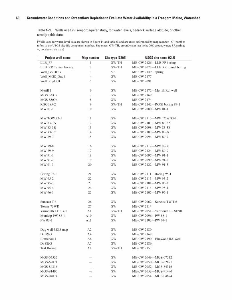
60 Groundwater Conditions and Streamflow Depletion to Evaluate Water Availability in a Freeport, Maine, Watershed
Table 1–1. Wells used in Freeport aquifer study, for water levels, bedrock surface altitude, or other stratigraphic data.—Continued
[Wells used for water-level data are shown in figure 14 and table 6, and are cross referenced by map number. “C”-number refers to the USGS site-file component number. Site types: GW-TH, groundwater test hole; GW, groundwater; SP, spring; --, not shown on map]
Project well name Map number Site type (C802) USGS site name (C12)LLB_FP 1 GW-TH ME-CW 2126—LLB FP boringLLB_RR Tunnel boring 2 GW-TH ME-CW 2072—LLB RR tunnel boringWell_GolDUG 3 SP ME-CW 2149—springWell_MGS_Dug1 4 GW ME-CW 2177Well_RogDUG 5 GW ME-CW 2091
Merill 1 6 GW ME-CW 2172—Merrill Rd. wellMGS S&Ga 7 GW ME-CW 2169MGS S&Gb 8 GW ME-CW 2174RGGI 85-2 9 GW-TH ME-CW 2142—RGGI boring 83-1MW 01-1 10 GW ME-CW 2080—MW 01-1
MW TOW 83-1 11 GW ME-CW 2110—MW TOW 83-1MW 83-3A 12 GW ME-CW 2103—MW 83-3AMW 83-3B 13 GW ME-CW 2098—MW 83-3BMW 83-3C 14 GW ME-CW 2107—MW 83-3CMW 89-7 15 GW ME-CW 2094—MW 89-7
MW 89-8 16 GW ME-CW 2117—MW 89-8MW 89-9 17 GW ME-CW 2124—MW 89-9MW 91-1 18 GW ME-CW 2097—MW 91-1MW 91-2 19 GW ME-CW 2099—MW 91-2MW 91-3 20 GW ME-CW 2122—MW 91-3
Boring 95-1 21 GW ME-CW 2111—Boring 95-1MW 95-2 22 GW ME-CW 2115—MW 95-2MW 95-3 23 GW ME-CW 2101—MW 95-3MW 95-4 24 GW ME-CW 2116—MW 95-4MW 96-1 25 GW ME-CW 2105—MW 96-1
Suneast T-6 26 GW ME-CW 2062—Suneast TW T-6Towns 73WR 27 GW ME-CW 2114Yarmouth LF SB90 A1 GW-TH ME-CW 2051—Yarmouth LF SB90Municip PW 88-1 A10 GW ME-CW 2096—PW 88-1PW 03-1 A11 GW ME-CW 2102—PW 03-1
Dug well MGS map A2 GW ME-CW 2180Dr S&G A4 GW ME-CW 2168Elmwood 1 A6 GW ME-CW 2190—Elmwood Rd. wellDr S&G A7 GW ME-CW 2189Test Boring A8 GW-TH ME-CW 2157
MGS-07532 -- GW ME-CW 2049—MGS-07532MGS-62871 -- GW ME-CW 2050—MGS-62871MGS-84316 -- GW ME-CW 2052—MGS-84316MGS-91490 -- GW ME-CW 2053—MGS-91490MGS-04874 -- GW ME-CW 2054—MGS-04874

Appendix 1 61
Table 1–1. Wells used in Freeport aquifer study, for water levels, bedrock surface altitude, or other stratigraphic data.—Continued
[Wells used for water-level data are shown in figure 14 and table 6, and are cross referenced by map number. “C”-number refers to the USGS site-file component number. Site types: GW-TH, groundwater test hole; GW, groundwater; SP, spring; --, not shown on map]
Project well name Map number Site type (C802) USGS site name (C12)MGS-64767 -- GW ME-CW 2055—MGS-64767MGS-09224 -- GW ME-CW 2056—MGS-09224MGS-60059 -- GW ME-CW 2057—MGS-60059MGS-04871 -- GW ME-CW 2058—MGS-04871MGS-06624 -- GW ME-CW 2059—MGS-06624
MGS-08087 -- GW ME-CW 2060—MGS-08087MGS-55577 -- GW ME-CW 2061—MGS-55577MGS-51612 -- GW ME-CW 2063—MGS-51612MGS-06623 -- GW ME-CW 2064—MGS-06623MGS-73687 -- GW ME-CW 2065—MGS-73687
MGS-10240 -- GW ME-CW 2066—MGS-10240MGS-55513 -- GW ME-CW 2067—MGS-55513MGS-07565 -- GW ME-CW 2068—MGS-07565MGS-55440 -- GW ME-CW 2069—MGS-55440MGS-62149 -- GW ME-CW 2070—MGS-62149
MGS-65380 -- GW ME-CW 2071—MGS-65380BR -- GW ME-CW 2073MGS-62146 -- GW ME-CW 2074—MGS-62146MGS-66301 -- GW ME-CW 2075—MGS-66301MGS-71795 -- GW ME-CW 2076—MGS-71795
MGS-62145 -- GW ME-CW 2077—MGS-62145MGS-60538 -- GW ME-CW 2078—MGS-60538MGS-06044 -- GW ME-CW 2079—MGS-06044MGS-76243 -- GW ME-CW 2081—MGS-76243MGS-56491 -- GW ME-CW 2082—MGS-56491
MGS-08630 -- GW ME-CW 2083—MGS-08630MGS-122361 -- GW ME-CW 2084—MGS-122361BR -- GW ME-CW 2085MGS-71719 -- GW ME-CW 2086—MGS-71719MGS-55621 -- GW ME-CW 2087—MGS-55621
MGS-07497 -- GW ME-CW 2088—MGS-07497MGS-07400 -- GW ME-CW 2089—MGS-07400MGS-64771 -- GW ME-CW 2090—MGS-64771LLBean B115 -- GW-TH ME-CW 2092—LLB B115MGS-51536 -- GW ME-CW 2093—MGS-51536
LLBean B110 -- GW-TH ME-CW 2095—LLB B110MGS-07399 -- GW ME-CW 2100—MGS-07399Sutton BR -- GW ME-CW 2104TW 8-in (97-1) -- GW ME-CW 2106—TW 97-1MGS-55630 -- GW ME-CW 2108—MGS-55630

62 Groundwater Conditions and Streamflow Depletion to Evaluate Water Availability in a Freeport, Maine, Watershed
Table 1–1. Wells used in Freeport aquifer study, for water levels, bedrock surface altitude, or other stratigraphic data.—Continued
[Wells used for water-level data are shown in figure 14 and table 6, and are cross referenced by map number. “C”-number refers to the USGS site-file component number. Site types: GW-TH, groundwater test hole; GW, groundwater; SP, spring; --, not shown on map]
Project well name Map number Site type (C802) USGS site name (C12)LLBean B104 -- GW-TH ME-CW 2109—LLB B104LLBean B101 -- GW-TH ME-CW 2112—LLB B101MW 83-2 -- GW ME-CW 2113—MW 83-2MGS-07292 -- GW ME-CW 2118—MGS-07292MGS-08466 -- GW ME-CW 2119—MGS-08466
MGS-07724 -- GW ME-CW 2120—MGS-07724Batch 90WR -- GW ME-CW 2121MGS-78537 -- GW ME-CW 2123—MGS-78537MGS-84441 -- GW ME-CW 2125—MGS-84441Weeks 89WR -- GW ME-CW 2127
MGS-08976 -- GW ME-CW 2128—MGS-08976BR -- GW ME-CW 2129Washburn -- GW ME-CW 2130MGS-52271 -- GW ME-CW 2131—MGS-52271MGS-08743 -- GW ME-CW 2132—MGS-08743
MGS-53568 -- GW ME-CW 2133—MGS-53568MGS-100343 -- GW ME-CW 2134—MGS-100343BR -- GW ME-CW 2135BR -- GW ME-CW 2136MGS-100342 -- GW ME-CW 2137—MGS-100342
MGS-07398 -- GW ME-CW 2138—MGS-07398MGS-128657 -- GW ME-CW 2139—MGS-128657MGS-101075 -- GW ME-CW 2140—MGS-101075MGS-07513 -- GW ME-CW 2141—MGS-07513MGS-60016 -- GW ME-CW 2143—MGS-60016
MGS-05053 -- GW ME-CW 2144—MGS-05053MGS-61559 -- GW ME-CW 2145—MGS-61559MGS-09932 -- GW ME-CW 2146—MGS-09932MGS-67014 -- GW ME-CW 2147—MGS-67014MGS-61812 -- GW ME-CW 2148—MGS-61812
MGS-06635 -- GW ME-CW 2150—MGS-06635MGS-10001 -- GW ME-CW 2151—MGS-10001BR -- GW ME-CW 2152MGS-60046 -- GW ME-CW 2153—MGS-60046BR -- GW ME-CW 2154
MGS-80936 -- GW ME-CW 2155—MGS-80936BR -- GW ME-CW 2156MGS-58053 -- GW ME-CW 2158—MGS-58053MGS-81983 -- GW ME-CW 2159—MGS-81983MGS-99680 -- GW ME-CW 2160—MGS-99680

Appendix 1 63
Table 1–1. Wells used in Freeport aquifer study, for water levels, bedrock surface altitude, or other stratigraphic data.—Continued
[Wells used for water-level data are shown in figure 14 and table 6, and are cross referenced by map number. “C”-number refers to the USGS site-file component number. Site types: GW-TH, groundwater test hole; GW, groundwater; SP, spring; --, not shown on map]
Project well name Map number Site type (C802) USGS site name (C12)MGS-103038 -- GW ME-CW 2161—MGS-103038MGS-67043 -- GW ME-CW 2162—MGS-67043MGS-08261 -- GW ME-CW 2163—MGS-08261MGS-78105 -- GW ME-CW 2164—MGS-78105MGS-08624 -- GW ME-CW 2165—MGS-08624
MGS-08114 -- GW ME-CW 2166—MGS-08114MGS-58368 -- GW ME-CW 2167—MGS-58368MGS-61081 -- GW ME-CW 2170—MGS-61081MGS-67572 -- GW ME-CW 2171—MGS-67572MGS-78104 -- GW ME-CW 2173—MGS-78104
MGS-08763 -- GW ME-CW 2175—MGS-08763MGS-80412 -- GW ME-CW 2176—MGS-80412Dug -- GW ME-CW 2178MGS-82000 -- GW ME-CW 2179—MGS-82000MGS-84486 -- GW ME-CW 2181—MGS-84486
BR -- GW ME-CW 2182MGS-08858 -- GW ME-CW 2183—MGS-08858MGS-08213 -- GW ME-CW 2184—MGS-08213BR -- GW ME-CW 2185MGS-08076 -- GW ME-CW 2186—MGS-08076
MGS-87240 -- GW ME-CW 2187—MGS-87240BR -- GW ME-CW 2188MGS-09209 -- GW ME-CW 2191—MGS-09209MGS-09928 -- GW ME-CW 2192—MGS-09928MGS-66959 -- GW ME-CW 2193—MGS-66959
MGS-08357 -- GW ME-CW 2194—MGS-08357MGS-07563 -- GW ME-CW 2195—MGS-07563Dr S&G -- GW ME-CW 2196MGS-07514 -- GW ME-CW 2197—MGS-07514Dug -- GW ME-CW 2198
MGS-08358 -- GW ME-CW 2199—MGS-08358MGS-110758 -- GW ME-CW 2200—MGS-110758MGS-98995 -- GW ME-CW 2201—MGS-98995MGS-58390 -- GW ME-CW 2202—MGS-58390MGS-81960 -- GW ME-CW 2203—MGS-81960
MGS-05933 -- GW ME-CW 2204—MGS-05933MGS-05945 -- GW ME-CW 2205—MGS-05945BR -- GW ME-CW 2206
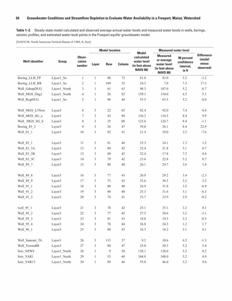
64 Groundwater Conditions and Streamflow Depletion to Evaluate Water Availability in a Freeport, Maine, Watershed
Table 1–2. Steady-state model calculated and observed average annual water levels and measured water levels in wells, borings, seismic profiles, and estimated water-level points in the Freeport aquifer groundwater model.—Continued
[NAVD 88, North American Vertical Datum of 1988; ft, foot]
Well identifier GroupObser-vation
number
Model locationModel
calculated water level
(in feet above NAVD 88)
Measured water levelDifference
(model minus
observed)Layer Row Column
Measured or average water level
(in feet above NAVD 88)
90 percent confidence
interval, in ft
Boring_LLB_FP Layer1_So 1 1 88 72 81.8 83.0 5.2 -1.2Boring_LLB_RR Layer1_So 2 1 109 52 24.3 7.0 7.3 17.3Well_GdrupDUG Layer1_North 3 1 61 63 98.3 107.0 5.2 -8.7Well_MGS_Dug1 Layer1_North 4 1 26 82 159.1 154.0 6.5 5.1Well_RogDUG Layer1_So 5 1 88 44 55.5 63.5 5.2 -8.0
Well_MGS_L3New Layer3 6 3 22 65 92.4 92.0 7.4 0.4Well_MGS_SG_a Layer3 7 2 42 94 126.3 116.5 8.4 9.9Well_ MGS_SG_b Layer3 8 2 35 88 123.6 124.7 8.4 -1.1Boring_85_2 Layer3 9 3 56 47 59.0 36.1 8.4 22.9Well_01_1 Layer3 10 3 92 41 21.4 29.0 2.5 -7.6
Well_83_1 Layer3 11 3 81 46 25.3 24.1 1.3 1.2Well_83_3A Layer3 12 3 80 42 22.4 21.8 5.1 0.7Well_83_3B Layer3 13 3 80 42 22.4 17.8 7.2 4.6Well_83_3C Layer3 14 3 79 42 23.6 22.8 5.2 0.7Well_89_7 Layer3 15 3 80 40 26.1 24.7 2.6 1.4
Well_89_8 Layer3 16 3 77 43 26.9 29.2 3.4 -2.3Well_89_9 Layer3 17 3 73 43 33.6 30.3 3.2 3.3Well_91_1 Layer3 18 3 80 40 24.9 31.8 3.5 -6.9Well_91_2 Layer3 19 3 80 40 25.3 31.6 3.1 -6.3Well_91_3 Layer3 20 3 74 41 33.7 33.9 2.9 -0.2
well_95_1 Layer3 21 3 78 42 25.1 25.1 3.2 0.1Well_95_2 Layer3 22 3 77 42 27.5 30.6 3.2 -3.1Well_95_3 Layer3 23 3 81 43 18.8 19.3 2.2 -0.5Well_95_4 Layer3 24 3 78 44 26.0 24.3 1.2 1.7Well_96_1 Layer3 25 3 80 43 16.3 16.2 2.1 0.1
Well_Suneast_T6 Layer3 26 3 115 37 9.2 10.6 6.5 -1.3Well_TownsBR Layer3 27 3 80 47 25.8 20.3 5.2 5.4Seis_NPW8 Layer1_North 28 1 9 58 128.1 128.0 5.2 0.2Seis_YAR1 Layer1_North 29 1 53 60 104.9 100.0 5.2 4.9Seis_YAR13 Layer1_North 30 1 89 46 55.0 46.0 5.2 9.0

Appendix 1 65
Table 1–2. Steady-state model calculated and observed average annual water levels and measured water levels in wells, borings, seismic profiles, and estimated water-level points in the Freeport aquifer groundwater model.—Continued
[NAVD 88, North American Vertical Datum of 1988; ft, foot]
Well identifier GroupObser-vation
number
Model locationModel
calculated water level
(in feet above NAVD 88)
Measured water levelDifference
(model minus
observed)Layer Row Column
Measured or average water level
(in feet above NAVD 88)
90 percent confidence
interval, in ft
Seis_YMH1 Layer1_North 31 1 70 48 56.0 49.0 5.2 7.0Seis_YMH15 Layer1_So 32 1 101 44 44.0 45.0 5.2 -1.0Seis_YMH16 Layer1_So 33 1 103 46 43.2 43.0 5.2 0.1Seis_YMH17 Layer1_So 34 1 97 47 48.0 52.0 5.2 -4.1Seis_YMH18 Layer1_So 35 1 100 46 45.9 46.0 5.2 -0.1
Seis_YMH19 Layer1_So 36 1 98 45 47.2 52.0 5.2 -4.8Seis_YMH2 Layer1_North 37 1 67 48 78.5 88.0 5.2 -9.5Seis_YMH20 Layer1_So 38 1 92 47 51.9 54.0 5.2 -2.1Seis_YMH3 Layer1_North 39 1 65 57 68.0 58.0 5.2 10.0Seis_YMH4 Layer1_North 40 1 49 78 137.7 151.0 5.2 -13.3
Seis_YMH5 Layer1_North 41 1 55 62 107.0 119.0 5.2 -12.0Seis_YMH7 Layer1_North 42 1 32 71 120.3 119.0 5.2 1.3Seis_YMH8 Layer1_North 43 1 55 50 98.1 87.0 5.2 11.1Syn_Till1 Estimated 44 1 114 20 35.3 39.7 8.4 -4.4Syn_Till10 Estimated 45 1 9 42 118.3 137.1 8.4 -18.9
Syn_Till11 Estimated 46 1 63 81 190.9 200.1 8.4 -9.2Syn_Till2 Estimated 47 1 136 35 48.2 54.8 8.4 -6.5Syn_Till3 Estimated 48 1 141 26 55.8 59.4 8.4 -3.6Syn_Till4 Estimated 49 1 122 14 55.8 56.4 8.4 -0.7Syn_Till5 Estimated 50 2 137 11 29.9 25.6 8.4 4.3
Syn_Till6 Estimated 51 1 114 36 27.8 31.0 8.4 -3.2Syn_Till7 Estimated 52 2 99 71 80.4 76.8 8.4 3.6Syn_Till8 Estimated 53 1 82 57 74.7 67.9 8.4 6.8Syn_Till9 Estimated 54 1 75 73 159.0 135.2 8.4 23.8

THIS PAGE INTENTIONALLY LEFT BLANK

Appendix 2 67
Appendix 2. Details of Groundwater Model Calibration
Parameter Estimation and Model Calibration ................................................................................68Model Sensitivity Analysis ................................................................................................................71
Tables 2–1. Hydrogeologic units and corresponding model parameters for hydraulic properties,
with their calibrated hydraulic conductivities .......................................................................68 2–2. Streambed hydraulic conductivity model parameters and calibrated hydraulic
properties .....................................................................................................................................69 2–3. Recharge model parameters and calibrated recharge values ...........................................69 2–4. Model parameters and final composite scaled sensitivities and correlations used to
determine which parameters to estimate using parameter estimation ............................70 2–5. Dimensionless scaled sensitivities for observations, by parameter, for head
observation groups as a measure of model sensitivity in the Freeport aquifer groundwater flow model, Freeport, Maine .............................................................................72
2–6. Dimensionless scaled sensitivities for observations, by parameter, for streamflow observations as a measure of model sensitivity in the Freeport aquifer groundwater flow model, Freeport, Maine .....................................................................................................72

68 Groundwater Conditions and Streamflow Depletion to Evaluate Water Availability in a Freeport, Maine, Watershed
This appendix presents additional details about the cali-bration and sensitivity analysis of the Freeport aquifer ground-water flow model. Details about the parameters and their final values and sensitivities are presented, along with a table showing the complete list of simulated compared to observed values for the observations. In addition, detailed information on the sensitivity of the model, including the streamflow simu-lations, to the various parameters is discussed.
Parameter Estimation and Model Calibration
The groundwater flow model of the Freeport aquifer was calibrated using a combination of parameter estimation and trial-and-error adjustments to the model variables. Methods outlined in Hill and Tiedeman (2007) were followed during calibration, which uses a regression method as programmed in the UCODE_2005 software package (Poeter and others, 2008). The regression method compares alternative parameter values to the model fit, defined as the best match between observations and their simulated equivalents. The match is quantified using an objective function (Hill and Tiedeman, 2007; Poeter and others, 2008), and the software tests many
variations of parameter values to minimize the overall objec-tive function. This method allows for (1) the explicit account-ing of uncertainty in both the water levels and streamflows used as calibration targets, (2) the documentation of model sensitivity to model variables and to data used in the model. During the prediction phase, this method assists the user in documenting the uncertainty in the model predictions.
Model variables including hydraulic properties (horizon-tal and vertical hydraulic conductivity, table 2–1), streambed conductance (table 2–2), and recharge (table 2–3) were used as parameters in the model. Head and streamflow measure-ments were used for the calibration targets, or observations. Statistics indicating the fit of the model to the observed values (the ability of the model to reproduce the observations) were used as the dependent variables in the parameter estimation, whereas the model parameters are treated as independent variables through a series of linear and nonlinear regression calculations. The optimization of the parameter values was conducted through an iterative process in which the output of each iteration was used to determine which parameters could be estimated and whether trial-and-error changes to other parameters, or changes to the conceptual model were needed.
Appendix 2. Details of Groundwater Model Calibration
Table 2–1. Hydrogeologic units and corresponding model parameters for hydraulic properties, with their calibrated hydraulic conductivities.
[Model parameters shown in bold were set by parameter estimation. Kv, vertical hydraulic conductivity; Kh, horizontal hydraulic conductivity; ft/d, foot per day; Fm., Formation; NA, not applicable]
Unit description LayerKh parameter
name
Calibrated Kh,
in ft/dKv parameter name
Calibrated Kv,
in ft/d
Surficial sandy deposits above Presumpscot Fm. 1 HK_Lay1_A 13.6 VK_Sandy 3.28Surficial sandy deposits, eolian 1 HK_Lay1_A 13.6 VK_Sandy 3.28Till and weathered Presumpscot Fm., undivided 1 HK_Lay1_C .69 VK_Till 1.64Weathered Presumpscot Fm. silt/clay 1 HK_Lay1_CD 10.7 VK_Till 1.64Unweathered Presumpscot Fm. silt/clay 1 HK_Lay1_D .56 VK_ClayL1 .16Holocene alluvium and fine sand 1 HK_Lay1_B1 1.6 VK_Sandy 3.28Till and weathered Presumpscot Fm., undivided 2 HK_Lay2_TL 9.0 VK_Till2 .98Unweathered Presumpscot Fm. silt/clay 2 HK_Lay2_CL .00003 VK_Clay_L2 .000003Vertical flow zones in Presumpscot Fm. silt/clay 2 NA NA VK_C_FracN, VK_C_FracS 9.84, 2.46Fine sand, buried aquifer 3 HK_Lay3_Sa 18.1 VK_Lay3 16.4Coarse sand unit A 3 HK_Lay3_K2 150 VK_Lay3 16.4Coarse sand unit B 3 HK_Lay3_K3 167 VK_Lay3 16.4General head boundary, north 3 GHB_ParN 241 NA NAGeneral head boundary, south 3 GHB_ParS 241 NA NA
1The model was sensitive to this parameter, but it was highly correlated with a recharge parameter, and was set by hand.

Appendix 2 69
During the optimization process, the sensitivity of the model to each parameter value was determined for each optimization iteration, and only parameters that exceeded a threshold sen-sitivity (and were not highly correlated with each other) were estimated. Insensitive or highly correlated parameters were set and adjusted manually using a trial and error process. Hill and Tiedeman (2007) provide further details on the process of parameter estimation.
Twelve of the 33 parameters set up for the model were determined by parameter estimation, and the others were set manually (table 2–4). The final set of parameters is listed in table 2–4, along with their composite scaled sensitivities and significant correlations between parameters. Generally, parameters with composite scaled sensitivities greater than 0.5 can be estimated (Hill and Tiedeman, 2007), provided they are
not highly correlated with other estimated parameters. This guidance was followed for all parameters except RCH_DOM, which was set by hand because the estimation routine yielded values above the reasonable maximum recharge for the area.
The Kv values were set by hand at the beginning of the calibration phase (with the exception of two enhanced vertical conductance zones in layer 2, discussed next) based on reason-able values from literature, and only those that displayed a minimal amount of sensitivity were adjusted during calibration using trial-and-error methods. This resulted in some Kv values being larger than the corresponding Kh values for the same unit, but because of the insensitivity of the model to those Kv parameters, this inconsistency was considered acceptable. The model was not very sensitive to the Kv parameters, and none were set by parameter estimation.
Table 2–2. Streambed hydraulic conductivity model parameters and calibrated hydraulic properties.
[Values in bold were determined using parameter estimation; ft/d, foot per day; Kdr, streambed hydraulic conductivity]
Streambed hydraulic conductance zonesKdr parameter
nameCalibrated Kdr,
in ft/d
Harvey Brook valley bottom areas, south part of the valley. KDR_Har1 1.5Headwaters of Harvey Brook watershed. Mixed surficial geology, primarily sandy with
some weathered clay areas.KDR_HarUp 4.5
Upland areas in Harvey Brook watershed, where streams are intermittent. KDR_HarMix .02Harvey Brook valley adjacent to eolian sands. KDR_HarSan 5Merrill Brook watershed uplands and some areas near stream. KDR_Merrill .017Cousins River valley bottom areas, and other areas with saturated Presumpscot Fm.
near surface. Cousins River valley has significant estuarine marsh sediments as well.KDR_ClyBot 1.5
Table 2–3. Recharge model parameters and calibrated recharge values.
[Values in bold were determined using parameter estimation; in/yr, inch per year]
Recharge zonesRecharge parameter
name
Calibrated recharge,
in in/yr
Uplands with till and (or) weathered Presumpscot Fm. soils. RCH_Till 5.037Cousins River valley bottom areas, and other areas with saturated Presumpscot Fm near surface. RCH_Clay .75Area of high slope at western edge of model, where runoff from upland areas can enter subsurface
through short losing stream reaches.RCH_HSL1 50
Areas of eolian sands, and Harvey Brook valley adjacent to those areas. RCH_DOM2 24Areas where surficial units above bedrock are 10 ft thick or less. RCH_Thin2 7.1Upland areas in Harvey Brook watershed, where streams are intermittent, soils primarily sandy. RCH_SandyN 10.75Upland areas on either side of Harvey Brook and to the south of the eolian sand deposits where
nearshore marine sandy units are present.RCH_SandyS 25
1The model was sensitive to this parameter, but parameter estimation yielded values outside the reasonable range, so it was set by hand.2The model was sensitive to this parameter, but it was highly correlated with a hydraulic conductivity parameter, and was set by hand.

70 Groundwater Conditions and Streamflow Depletion to Evaluate Water Availability in a Freeport, Maine, Watershed
Table 2–4. Model parameters and final composite scaled sensitivities and correlations used to determine which parameters to estimate using parameter estimation.
[--, none significant]
Parameter nameComposite scaled
sensitivityCorrelations with other parameters
Set using parameter
estimation?
RCH_SandyS 5.58 -- YesHK_Lay3_Sa 2.63 -- YesRCH_DOM 2.54 -- NoRCH_Thin 2.49 HK_Lay1_C NoKDR_Merill 2.28 -- YesRCH_Till 2.26 -- YesRCH_SandyN 2.15 HK_Lay1_B YesHK_Lay1_C 2.15 RCH_Thin YesHK_Lay1_A 1.63 -- YesHK_Lay1_B 1.51 RCH_SandyN NoHK_Lay3_K2 1.27 -- YesHK_Lay2_TL 1.15 -- YesHK_Lay1_CD 1.14 -- YesRCH_HSL .97 -- NoHK_Lay3_K3 .95 -- YesHK_Lay1_D .78 -- YesKDR_HarUp .34 -- NoVK_C_FracS .29 VK_C_FracN; VK_Lay3 NoKDR_Har1 .29 VK_Lay3; VK_C_FracN NoKDR_HarSan .27 -- NoKDR_HarMix .20 -- NoVK_C_FracN .15 VK_C_FracS; VK_Lay3; KDR_Har1 NoKDR_ClyBot .15 -- NoVK_Lay3 6.62 × 10⁻² VK_C_FracS; VK_C_FracN; KDR_Har1 NoVK_Sandy 6.23 × 10⁻² -- NoVK_ClayL1 3.73 × 10⁻² -- NoVK_TillL2 2.91 × 10⁻² -- NoRCH_Clay 2.62 × 10⁻² -- NoVK_Till 1.79 × 10⁻² -- NoVK_ClayL2 1.63 × 10⁻² -- NoHK_Lay2_Cl 1.54 × 10⁻² -- NoGHB_ParN 5.25 × 10⁻³ -- NoGHB_ParS 3.30 × 10⁻⁴ -- No

Appendix 2 71
Model Sensitivity Analysis
The sensitivity of the model results to the numerous model variables and parameters was tested in UCODE_2005. The UCODE_2005 output can report the sensitivity of the observations to the optimized parameters and the parameters set by hand. Dimensionless scaled sensitivities calculated by UCODE_2005 indicate how much an observation would change given a 1-percent change in the parameter value, scaled by the error in the observation (Hill and Tiedeman, 2007, p. 49). The sensitivity values for every parameter/vari-able are reported for each observation; these observations can be grouped according to their use and position in the model, as observations representing similar parts of the model geometry are sensitive to similar parameters. Although the dimension-less scaled sensitivity is a “fit-independent” statistic, the analy-sis was run using the optimal parameter values for the model. The parameters of greatest importance to the simulation have the largest absolute values (Hill and Tiedeman, 2007, p. 49).
The sensitivity of the model results to the input variables is summarized in tables 2–5 and 2–6. This summary presents the average of the absolute values of the dimensionless scaled sensitivities for parameters in three groups of head observa-tions and the individual streamflow observations. The observa-tion groups in table 2–5 are Layer 1&2 north (observations in wells, borings, and seismic lines in the surficial units above the confining unit and north of the pumping wells), Layer 1&2 south (observations in wells, borings, and seismic lines in the surficial units south of the pumping wells), and Layer 3 (all head observations in layer 3). Table 2–6 contains the sensitivities for the streamflow observations. In both tables, parameters that had minimal sensitivities to the observations were not listed. The heads in both zones of the surficial units (Layer 1&2 north and Layer 1&2 south) were sensitive to the KDR_Merrill, RCH_SandyS, HK_Lay1_A, and HK_Lay1_B parameters. The northern surficial heads were also quite
sensitive to the recharge parameters RCH_DOM and RCH_SandyN, as well as the HK_Lay1_CD hydraulic conductivity parameter. The southern surficial heads were sensitive to the RCH_Thin, RCH_Till, and HK_Lay1_C parameters. Layer 3 heads were most sensitive to the hydraulic conductivity zones in layer 3 (HK_Lay3_Sa, HK_Lay3_K2, and HK_Lay3_K3), and the recharge parameters RCH_HSL and RCH_SandyS, and to a lesser extent the recharge parameters RCH_Till and RCH_DOM. None of the heads were very sensitive to recharge, Kh, or Kv in the clay units, to the Kh of the general head boundaries, to the Kv parameters in the till area, or to any other Kv parameters, including the Kv of the vertical con-ductance zones through the clay in layer 2. The streamflows were all sensitive to the recharge parameters RCH_Till and RCH_SandyS, although the Harvey Brook #2 site was particu-larly sensitive to the RCH_SandyS parameter. This outcome is likely because the site gets a larger proportion of its discharge from the upper sand unit than from the other Harvey Brook sites. Of the drain conductance parameters, KDR_Merrill had the greatest effect on the streamflows, even in the Harvey Brook watersheds, because this parameter had some control on the position of the groundwater divide between the water-sheds. Several of the streamflow observations were sensitive to the Kh parameters in layer 3, as these controlled the overall movement of water through layer 3 and toward the vertical conductance zones in the layer 2 clay. Also important in this movement of water was the recharge parameter RCH_HSL, to which the Harvey Brook sites were all sensitive. Parameters that the streamflow observations were insensitive to included the following: recharge; Kh, or Kv in the clay units (with the exception of the vertical conductance zone VK_C_FracS through the clay in layer 2); the Kh of the general head bound-aries; and the Kv parameters in the till area, or any other Kv parameters. Streamflows were also relatively insensitive to the KDR_HarUp, KDR_ClyBot, and KDR_HarSan streamflow conductance parameters.

72 Groundwater Conditions and Streamflow Depletion to Evaluate Water Availability in a Freeport, Maine, WatershedTa
ble
2–5.
Di
men
sion
less
sca
led
sens
itivi
ties
for o
bser
vatio
ns, b
y pa
ram
eter
, for
hea
d ob
serv
atio
n gr
oups
as
a m
easu
re o
f mod
el s
ensi
tivity
in th
e Fr
eepo
rt aq
uife
r gr
ound
wat
er fl
ow m
odel
, Fre
epor
t, M
aine
.
[Par
amet
ers n
ot li
sted
hav
e ne
glig
ible
sens
itivi
ty. B
old
valu
es a
re th
e hi
ghes
t 8 fo
r eac
h ob
serv
atio
n gr
oup]
Hea
d ob
serv
atio
n gr
oup
Num
ber o
f ob
serv
atio
ns
in g
roup
Aver
age
dim
ensi
onle
ss s
cale
d se
nsiti
vitie
s (a
bsol
ute
valu
es) p
er o
bser
vatio
n in
eac
h gr
oup
HK_Lay3_Sa
HK_Lay2_TL
KDR_Merill
KDR_HarSan
RCH_Till
RCH_HSL
RCH_DOM
RCH_Thin
RCH_SandyN
RCH_SandyS
HK_Lay3_K2
HK_Lay1_A
HK_Lay1_B
HK_Lay1_C
HK_Lay1_CD
HK_Lay1_D
HK_Lay3_K3
Laye
r 1&
2 no
rth12
0.78
0.33
0.46
0.12
0.43
0.03
2.68
0.38
1.75
1.37
0.05
1.79
0.86
0.22
1.64
0.04
0.02
Laye
r 1&
2 so
uth
90.
090.
073.
610.
010.
570.
020.
062.
000.
007.
230.
011.
322.
151.
530.
010.
560.
00
Laye
r 322
2.76
0.10
0.23
0.31
0.42
1.15
0.30
0.09
0.09
1.57
1.01
0.19
0.24
0.01
0.25
0.01
1.27
Synt
hetic
till
111.
001.
361.
130.
034.
150.
040.
860.
580.
402.
920.
021.
090.
192.
460.
181.
130.
02
Tabl
e 2–
6.
Dim
ensi
onle
ss s
cale
d se
nsiti
vitie
s fo
r obs
erva
tions
, by
para
met
er, f
or s
tream
flow
obs
erva
tions
as
a m
easu
re o
f mod
el s
ensi
tivity
in th
e Fr
eepo
rt aq
uife
r gr
ound
wat
er fl
ow m
odel
, Fre
epor
t, M
aine
.
[Par
amet
ers n
ot li
sted
hav
e ne
glig
ible
sens
itivi
ty. B
old
valu
es a
re th
e hi
ghes
t 8 fo
r eac
h ob
serv
atio
n]
Stre
amflo
w
obse
rvat
ion
Stat
ion
Indi
vidu
al d
imen
sion
less
sca
led
sens
itivi
ties
(abs
olut
e va
lues
)
HK_Lay3_Sa
KDR_Merill
KDR_HarMix
KDR_Har1
RCH_Till
RCH_HSL
RCH_DOM
RCH_Thin
VK_C_FracS
RCH_SandyN
RCH_SandyS
HK_Lay3_K2
HK_Lay1_A
HK_Lay1_B
HK_Lay1_C
HK_Lay3_K3
Har
vey
Bro
ok 1
12.
911.
460.
021.
851.
121.
840.
310.
141.
740.
029.
510.
700.
930.
770.
031.
79
Har
vey
Bro
ok 2
21.
715.
780.
720.
310.
772.
080.
190.
040.
340.
0120
.41
0.25
0.44
5.58
0.18
0.84
Har
vey
Bro
ok 3
30.
691.
130.
010.
170.
723.
427.
750.
120.
180.
755.
326.
150.
420.
110.
141.
45
Har
vey
Bro
ok 4
42.
950.
180.
000.
012.
440.
428.
751.
830.
019.
251.
200.
750.
380.
260.
150.
04
Mer
rill B
rook
50.
816.
550.
210.
052.
470.
040.
423.
040.
050.
008.
920.
010.
861.
761.
040.
05

Prepared by the Pembroke, Raleigh, and Rolla Publishing Service Centers.
For more information concerning this report, contact:
DirectorU.S. Geological SurveyMaine Water Science Center196 Whitten RoadAugusta, ME [email protected]
or visit our Web site at:http://me.water.usgs.gov

Nielsen and Locke—
Groundw
ater Conditions and Streamflow
Depletion to Evaluate W
ater Availability in a Freeport, Maine, W
atershed—SIR 2011–5227