J Econ Growth (2016) 21:1–33DOI 10.1007/s10887-015-9122-3

Premature deindustrialization

Dani Rodrik1

Published online: 27 November 2015© Springer Science+Business Media New York 2015

Abstract I document a significant deindustrialization trend in recent decades that goes con-siderably beyond the advanced, post-industrial economies. The hump-shaped relationshipbetween industrialization (measured by employment or output shares) and incomes hasshifted downwards and moved closer to the origin. This means countries are running outof industrialization opportunities sooner and at much lower levels of income compared to theexperience of early industrializers. Asian countries and manufactures exporters have beenlargely insulated from those trends, while Latin American countries have been especiallyhard hit. Advanced economies have lost considerable employment (especially of the low-skill type), but they have done surprisingly well in terms of manufacturing output sharesat constant prices. While these trends are not very recent, the evidence suggests both glob-alization and labor-saving technological progress in manufacturing have been behind thesedevelopments. The paper briefly considers some of the economic and political implicationsof these trends.

Keywords Deindustrialization · Industrialization · Economic growth

JEL classification 014

1 Introduction

Our modern world is in many ways the product of industrialization. It was the industrialrevolution that enabled sustained productivity growth in Europe and the United States for thefirst time, resulting in the division of the world economy into rich and poor nations. It wasindustrialization again that permitted catch-up and convergence with the West by a relativelysmaller number of non-Western nations—Japan starting in the late Nineteenth century, SouthKorea, Taiwan and a few others after the 1960s. In countries that still remainmired in poverty,

B Dani Rodrikdani_rodrik@harvard.edu

1 John F. Kennedy School of Government, Harvard University, Cambridge, MA 02138, USA

123

2 J Econ Growth (2016) 21:1–33

such as those in sub-SaharanAfrica and southAsia,many observers and policymakers believefuture economic hopes rest in important part on fostering new manufacturing industries.

Most of the advanced economies of the world have long moved into a new, post-industrialphase of development. These economies have been deindustrializing for decades, a trendthat is particularly noticeable when one looks at the employment share of manufacturing.Employment deindustrialization has long been a concern in rich nations, where it is associatedin public discussions with the loss of good jobs, rising inequality, and a potential decline ininnovation capacity.1 In terms of output, deindustrialization has been in fact less strikingand uniform, a pattern that is obscured by the frequent reliance on value added measures atcurrent rather than constant prices.

In the United States manufacturing industries’ share of total employment has steadilyfallen since the 1950s, coming down from around a quarter of the workforce to less than atenth today. Meanwhile, manufacturing value-added (MVA) has remained a constant shareof GDP at constant prices—a testament to differentially rapid labor productivity growth inthis sector. In Great Britain, at the other end of the spectrum, deindustrialization has beenboth more rapid and thorough. Manufacturing’s share of employment has fallen from a thirdin the 1970s to slightly above 10 % today, while real MVA (at 2005 prices) has declined fromaround a quarter of GDP to less than 15 %.2 Across the developed world as a whole, realmanufacturing output has held its own rather well once we control for changes in incomeand population, as I will show later in the paper.

The term deindustrialization is used today to refer to the experience mainly of theseadvanced economies. In this paper, I focus on a less noticed trend over the last three decades,which is an even more striking, and puzzling, pattern of deindustrialization in low- andmiddle-income countries. With some exceptions, confined largely to Asia, developing coun-tries have experienced fallingmanufacturing shares in both employment and real value added,especially since the 1980s. For the most part, these countries had built up modest manufac-turing industries during the 1950s and 1960s, behind protective walls and under policies ofimport substitution. These industries have been shrinking significantly since then. The low-income economies of Sub-Saharan Africa have been affected nearly as much by these trendsas the middle-income economies of Latin America—though there was less manufacturing tobegin with in the former group of countries.

Manufacturing typically follows an inverted U-shaped path over the course of develop-ment. Even though such a pattern can be observed in developing countries as well, the turningpoint arrives sooner and at much lower levels of income today. In most of these countries,manufacturing has begun to shrink (or is on course for shrinking) at levels of income thatare a fraction of those at which the advanced economies started to deindustrialize.3 Devel-oping countries are turning into service economies without having gone through a properexperience of industrialization. I call this “premature deindustrialization.”4

There are two senses in which the shrinking of manufacturing in low and medium incomeeconomies can be viewed as premature. The first, purely descriptive, sense is that these

1 The bulk of R&D and patents originates from manufacturing. In Europe, for example, close to two-thirdsof business R&D spending is done in manufacturing even though the sector is responsible for only 14–15 %of employment and value added in aggregate (Veugelers 2013, p. 8).2 These numbers come from Timmer et al. (2014), which is the principal data source I will use in the paper.3 See also Amirapu and Subramanian (2015), who document premature deindustrialization within Indianstates.4 The term seems to have been first used by Dasgupta and Singh (2006), although Kaldor (1966) made muchearlier reference to early deindustrialization in the British context. I am grateful to Andre Nassif for the Kaldorreference.

123

J Econ Growth (2016) 21:1–33 3

economies are undergoing deindustrialization much earlier than the historical norms. As Iwill show in Sect. 6, late industrializers are unable to build as large manufacturing sectorsand are starting to deindustrialize at considerably lower levels of income, compared to earlyindustrializers.

The second sense in which this is premature is that early deindustrialization may havedetrimental effects on economic growth. Manufacturing activities have some features thatmake them instrumental in the process of growth. First, manufacturing tends to be techno-logically a dynamic sector. In fact, as demonstrated in Rodrik (2013), formal manufacturingsectors exhibit unconditional labor productivity convergence, unlike the rest of the economy.Second, manufacturing has traditionally absorbed significant quantities of unskilled labor,something that sets it apart from other high-productivity sectors such as mining or finance.Third, manufacturing is a tradable sector, which implies that it does not face the demandconstraints of a home market populated by low-income consumers. It can expand and absorbworkers even is the rest of the economy remains technologically stagnant. Taken together,these features make manufacturing the quintessential escalator for developing economies(Rodrik 2014). Hence early deindustrialization could well remove the main channel throughwhich rapid growth has taken place in the past. My focus in the present paper is on doc-umenting deindustrialization trends against the background of these considerations, ratherthan on examining their normative consequences.

I do spend some time to consider the underlying causes of these trends. I present a simpletheoretical framework in Sect. 7 to help interpret the key empirical findings of the paper. Twoimportant differences across country groups in particular need explanation. First, advancedcountries as a group have managed to avoid output deindustrialization, unlike the bulk ofdeveloping countries. Second, amongdeveloping countries,Asian countries have experiencedno output or employment deindustrialization. (Note that these patterns refer to outcomes afterincome and demographic trends are controlled for.) I do not attempt here a full-fledged causalexplanation for the patterns. But the model is suggestive of the combinations of technol-ogy and trade shocks that can account for the observed heterogeneity. In brief, productivityimprovements appear to have played the major role in the advanced economies, while glob-alization features more prominently in accounting for industrialization-deindustrializationpatterns within the developing world.

The conventional explanation for employment deindustrialization relies on differentialrates of technological progress (Lawrence and Edwards 2013). Typically, manufacturingexperiences more rapid productivity growth than the rest of the economy. This results in areduction in the share of the economy’s labor employed by manufacturing as long as theelasticity of substitution between manufacturing and other sectors is less than unity (σ < 1).As I show in Sect. 7, however, under the same assumptions the output share of manufacturingmoves in the opposite direction. To get both employment and output deindustrialization, weneed to make additional assumptions: that the trade balance in manufactures becomes morenegative or that there is a secular demand shift away frommanufactures. (The math is workedout in Sect. 7.)

Since the more pronounced story in the advanced countries is employment rather thanoutput deindustrialization, a technology-based story does reasonably well to account for thepatterns there. Further, the evidence suggests that a particular type of technological progress,of the unskilled-labor saving type, is responsible for the bulk of the labor displacement frommanufacturing (Sect. 5).

For developing countries, however, it is less evident that the technology argument appliesin quite the same way. Crucially, the mechanism referred to above relies on adjustments indomestic relative prices. Differential technological progress in manufacturing depresses the

123

4 J Econ Growth (2016) 21:1–33

relative price of manufacturing. In the case where σ < 1, this decline is sufficiently largethat it ensures demand for labor in manufacturing is lower in the new equilibrium. The bigdifference in developing countries is that they are small in world markets for manufactures,where they are essentially price takers. In the limit, when relative prices are fully determinedby global (rather than domestic) supply-demand conditions, more rapid productivity growthin manufacturing at home actually produces industrialization, not deindustrialization – interms of both employment and output (as the model of Sect. 7 shows). So the culprit fordeindustrialization in developing countries must be found elsewhere.

The obvious alternative is trade and globalization. A plausible story would be the follow-ing. As developing countries opened up to trade, their manufacturing sectors were hit by adouble shock. Those without a strong comparative advantage in manufacturing became netimporters of manufacturing, reversing a long process of import-substitution.5 In addition,developing countries “imported” deindustrialization from the advanced countries, becausethey became exposed to the relative price trends originating from advanced economies. Thedecline in the relative price of manufacturing in the advanced countries put a squeeze onmanufacturing everywhere, including the countries that may not have experienced muchtechnological progress. This account is consistent with the strong reduction in both employ-ment and output shares in developing countries (especially those that do not specialize inmanufactures). It also helps account for the fact that Asian countries, with a comparativeadvantage in manufactures, have been spared the same trends.

In sum, while technological progress is no doubt a large part of the story behind employ-ment deindustrialization in the advanced countries, in the developing countries trade andglobalization likely played a comparatively bigger role.

The outline of the paper is as follows. In Sect. 2, I discuss the data, various measuresof deindustrialization, and the inverse-U shaped relationship between industrialization andincomes. In Sects. 3 and 4, I document the patterns of deindustrialization over time and acrossdifferent country groups. In Sect. 5, I look at employment deindustrialization, differentiatingacross different labor types. In Sect. 6, I make the concept of premature deindustrializationmore precise. In Sect. 7, I develop an analytical framework within which the empirical resultscan be interpreted. In Sect. 8, I conclude.

2 The inverse U-shaped curve in manufacturing: data, measures andtrends

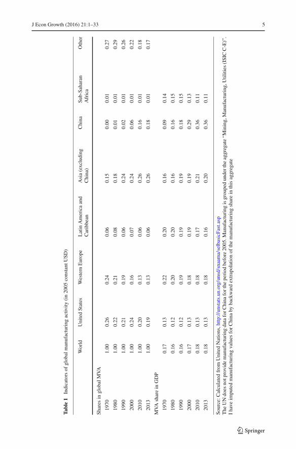
I begin by providing some indicators of changes in global manufacturing activity in recentdecades (Table 1). The data come from the United Nations and have globally comprehensivecoverage but they goback only to 1970. The top panel of the table shows the global distributionof manufacturing output, while the lower panel shows shares of manufacturing in GDP formajor regions. Two key conclusions stand out. First, there has been a significant relocationof manufacturing from the richer parts of the world (United States and Europe) to Asia,particularly China. Second, the share of manufacturing in GDP has moved differently invarious regions, and not always in a manner that would have been expected a priori. Somelow-income regions (sub-Saharan Africa and Latin America) have deindustrialized, whilesome high-income regions (namely the U.S.) have avoided that fate.

5 This echoes the concern in the voluminous literature on the Dutch disease, that developing countries withcomparative advantage in primary products would experience a squeeze on manufacturing as they open up totrade. See Corden (1984), van Wijnbergen (1984), and Sachs and Warner (1999).

123

J Econ Growth (2016) 21:1–33 5

Table1

Indicatorsof

glob

almanufacturing

activ

ity(in20

05constant

USD

)

World

UnitedStates

Western

Europe

Latin

Americaand

Caribbean

Asia(excluding

China)

China

Sub-Sa

haran

Africa

Other

Shares

inglobalMVA

1970

1.00

0.26

0.24

0.06

0.15

0.00

0.01

0.27

1980

1.00

0.22

0.21

0.08

0.18

0.01

0.01

0.29

1990

1.00

0.21

0.19

0.06

0.24

0.02

0.01

0.26

2000

1.00

0.24

0.16

0.07

0.24

0.06

0.01

0.22

2010

1.00

0.20

0.13

0.06

0.26

0.16

0.01

0.18

2013

1.00

0.19

0.13

0.06

0.26

0.18

0.01

0.17

MVAsharein

GDP

1970

0.17

0.13

0.22

0.20

0.16

0.09

0.14

1980

0.16

0.12

0.20

0.20

0.16

0.16

0.15

1990

0.16

0.12

0.19

0.19

0.19

0.18

0.15

2000

0.17

0.13

0.18

0.19

0.19

0.29

0.13

2010

0.18

0.13

0.18

0.17

0.21

0.36

0.11

2013

0.18

0.13

0.18

0.16

0.20

0.36

0.11

Source:C

alculatedfrom

UnitedNations,h

ttp://unstats.un.org/unsd/snaama/selbasicFast.asp

The

UNdo

esno

tprovide

manufacturing

dataforC

hina

forthe

period

before20

05.M

anufacturing

isgrou

pedun

derthe

aggregate“M

ining,Manufacturing

,Utilities

(ISICC-E)”.

Ihave

impu

tedmanufacturing

values

forChina

bybackwardextrapolationof

themanufacturing

sharein

thisaggregate

123

6 J Econ Growth (2016) 21:1–33

There are a variety of industrialization/deindustrializationmeasures in the literature. Somestudies focus on manufacturing employment (as a share of total employment), while othersuse manufacturing output (MVA as a share of GDP). MVA shares in turn can be calculated atconstant or current prices. Differentmeasures yield different trends and results. For complete-ness I will use all three measures in this paper, denoting them as manemp (manufacturingemployment share), nommva (MVA share at current prices), and realmva (MVA share atconstant prices). I will focus in later sections on the real magnitudes manemp and realmva,as nommva conflates movements in quantities and prices which are best kept distinct whentrying to understand patterns of structural change and their determinants.

Mybaseline results are based on data from theGroningenGrowth andDevelopmentCenter(GGDC, Timmer et al. 2014). These data span the period between the late 1940s/early 1950sthrough the early 2010s and cover 42 countries, both developed and developing. The majoreconomies in Latin America, Asia, and sub-Saharan Africa are included alongside advancedeconomies. (For more details on the data set, see the Appendix.) Constant-price series areat 2005 prices.6 For robustness checks and further analysis, I will supplement this datawith two other sources. The Socio-economic Accounts of the World Input-Output Database(Timmer 2012) provide a disaggregation of sectoral employment by three skill categoriesfor 40, mainly advanced economies. And researchers at the Asian Development Bank haverecently put together manufacturing employment and output series for a much larger groupof countries using a variety of sources, including the ILO, U.N., and World Bank, thoughthese data start from 1970 at the earliest (Felipe and Rhee 2014).7 I will combine thesevarious sources on manufacturing with income and population data from Maddison (2009),updated using the World Bank’s World Development Indicators. The income figures are at1990 international dollars.

Figure 1 shows the simulated relationship between the three measures of industrializationand income per capita. The figure is based on a quadratic estimation using country fixedeffects and controlling for population size and period dummies. (See Sect. 3 for the exactspecification.)The curves are drawn for a “representative” countrywith themedianpopulationin the sample (27 million). Period and country effects are all averaged to obtain a typicalrelationship for the sample and full time span covered. The estimation results underlyingthe figure are shown in Table 2, cols. (1)–(3). The quadratic terms are statistically highlysignificant for all three manufacturing indicators. The share of manufacturing tends to firstrise and then fall over the course of development.

However, the turning points differ significantly. In particular,manemp peaks much earlierthan realmva. The employment share of manufacturing starts to fall past an income levelof around $6,000 (in 1990 US)$, after having reached an estimated maximum close to 20%. Manufacturing output at constant prices peaks very late in the development process. Theestimated income level at which it begins to fall is in fact higher than any of the incomesobserved in the data set (above $70,000 in 1990 US)$.8 As we shall see in Sect. 6, post-1990

6 The only exception is West Germany, for which there are no data after 1991 and constant-price series areat 1991 prices. Since all my regressions include country fixed effects, this difference in base year will beabsorbed into the fixed effect for the country.7 I am grateful to Jesus Felipe for making these data available to me.8 These differences are statistically significant. The 95% confidence intervals for log incomes at which manu-facturing shares peak, computed using the delta method, are as follows: manemp [8.45, 8.97]; nommva [8.79,9.58], and realmva [10.16, 12.27]. The confidence interval for manemp (and nommva) does not overlap thatfor realmva. The series formanemp and nommva easily pass the Lind andMehlum (2010) test for the presenceof an inverse U-relationship in log GDP per capita, while realmva fails it because the extremum occurs outsidethe observed income range.

123

J Econ Growth (2016) 21:1–33 7

0

0.05

0.1

0.15

0.2

0.25

0.3

6 6.2

6.4

6.6

6.8 7 7.2

7.4

7.6

7.8 8 8.2

8.4

8.6

8.8 9 9.2

9.4

9.6

9.8 10 10.2

10.4

10.6

10.8 11 11.2

11.4

11.6

11.8 12

manemp

nommva

realmva

Fig. 1 Simulated manufacturing shares as a function of income (In GDP per capital in 1990 internationaldollars)

data indicate a much earlier decline, at less than half the pre-1990 income level. (Note thatthe peak shares themselves are less meaningful in the case of output, as they depend on thebase year selected for converting current prices to constant prices.)

The literature focuses on two possible explanations for whymanufacturing’s share eventu-ally falls (Ngai and Pissarides 2004; Buera and Joseph 2009; Foellmi and Zweimuller 2008;Lawrence and Edwards 2013; Nickell et al. 2008). One is demand-based, and relies on a shiftin consumption preferences away from goods and towards services. This on its own wouldnot produce the timing difference in peaks, as a pure demand shift would have similar effectson manufacturing quantities (output and employment). The second explanation is techno-logical, and relies on more rapid productivity growth in manufacturing than in the rest of theeconomy. As long as the elasticity of substitution is less than one, this produces a declinein the share of manufacturing employment, but not in the share of manufacturing output.We need a combination of supply- and demand-side reasons to explain both the decline inmanufacturing’s share and the later turnaround in output compared to employment.

An added complication is that the effects of technology and demand shocks depend cru-cially on whether the economy is open to trade or not (Matsuyama 2009). For the moment, Ileave these questions aside. I will develop the analytical results linking technology, demand,and trade to deindustrialization in Sect. 7.

As Fig. 1 shows, nommva also peaks much earlier than realmva, though not so early asmanemp. The explanation for this difference has to do with relative price changes over thecourse of development. The relative price of manufacturing tends to decline as countries getricher, tending to depress the share of MVA at current prices. Figure 2 displays the pattern forfour of the countries in our sample. The relative price of manufacturing has more than halvedin the United States since the early 1960s. Great Britain has experienced a somewhat smallerdecline. In South Korea, which has grown extremely rapidly, manufacturing’s relative price

123

8 J Econ Growth (2016) 21:1–33

Table2

Baselineregressions

Com

mon

sample

Largestsample

manem

pnommva

realmva

manem

pnommva

realmva

lnpo

pulatio

n0.11

5∗(0.021

)0.14

2∗(0.029

)−0

.113

∗ (0.02

8)0.12

2∗(0.021

)0.19

2∗(0.027

)−0

.039

(0.025

)

lnpo

pulatio

nsquared

−0.000

(0.001

)−0

.002

∗ (0.00

1)0.00

5∗(0.001

)−0

.001

(0.001

)−0

.004

∗ (0.00

1)0.00

3∗(0.001

)

lnGDPpercapita

0.32

1∗(0.027

)0.23

0∗(0.031

)0.20

4∗(0.025

)0.31

6∗(0.026

)0.26

6∗(0.031

)0.26

2∗(0.027

)

lnGDPpercapitasquared

−0.018

∗ (0.00

2)−0

.013

∗ (0.00

2)−0

.009

∗ (0.00

1)−0

.018

∗ (0.00

2)−0

.014

∗ (0.00

2)−0

.012

∗ (0.00

2)

1960

s−0

.029

∗ (0.00

5)−0

.011

∗∗∗ (

0.00

6)−0

.008

(0.005

)−0

.018

∗ (0.00

4)−0

.010

∗∗∗ (

0.00

6)−0

.028

∗ (0.00

7)

1970

s−0

.044

∗ (0.00

6)−0

.021

∗ (0.00

7)−0

.004

(0.006

)−0

.033

∗ (0.00

5)−0

.014

∗∗(0.007

)−0

.026

∗ (0.00

8)

1980

s−0

.066

∗ (0.00

7)−0

.033

∗ (0.00

8)−0

.011

∗∗∗ (

0.00

7)−0

.054

∗ (0.00

6)−0

.028

∗ (0.00

8)−0

.034

∗ (0.00

9)

1990

s−0

.086

∗ (0.00

9)−0

.052

∗ (0.00

9)−0

.017

∗∗(0.008

)−0

.074

∗ (0.00

8)−0

.049

∗ (0.00

9)−0

.040

∗ (0.01

0)

2000

s+−0

.117

∗ (0.01

0)−0

.085

∗ (0.01

0)−0

.035

∗ (0.00

9)−0

.105

∗ (0.00

9)−0

.085

∗ (0.01

0)−0

.059

∗ (0.01

1)

Country

fixed

effects

Yes

Yes

Yes

Yes

Yes

Yes

Num

berof

coun

tries

4242

4242

4242

Num

berof

observations

1995

1995

1995

2209

2128

2302

Robuststandarderrorsarereported

inparentheses

Levelsof

statistiticalsignficance:∗

99%;∗

∗ 95%;∗

∗∗90

%

123

J Econ Growth (2016) 21:1–33 9

12

34

rela

tive

pric

e de

flato

r of m

anuf

actu

ring

1960 1970 1980 1990 2000 2010Year

USA GBRKOR MEX

Fig. 2 Relative price trends

has come down by a whopping 250 %. In Mexico, meanwhile, relative prices have remainedmore or less flat.

These trends are also consistent broadly with a technology-based explanation for themanufacturing hump. More rapid productivity growth in manufacturing reduces the relativeprice of manufactured goods through standard supply-demand channels. This in turn causesnommva to reach an earlier peak than realmva as shown in Fig. 1.

3 Deindustrialization over time

As Fig. 1 makes clear, deindustrialization is the common fate of countries that are growing.My interest here is to checkwhether deindustrialization has beenmore rapid in recent periods.For this purpose, I use a basic specification that controls for the effect of demographic andincome trends (with quadratic terms for log population, pop, and GDP per capita, y) as wellas country fixed effects (Di ). The baseline regression looks as follows:

manshareit = β0 + β1 ln popit + β2 (ln popit )2 + β3 ln yit + β4 (ln yit )

2

+∑

iγi Di +

∑T

ϕT PERT + εi t ,

where manshare denotes one of our three indicators of industrialization. Country fixed-effects allow me to take into account any country-specific features (geography, endowments,history) that create a difference in the baseline conditions for manufacturing industry acrossdifferent nations. My main focus is on trends over time, which are captured using perioddummies (PERT ) for the 1960s, 1970s, 1980s, 1990s, and post-2000 years. (The post-2000dummy covers the period 2000 through the final year in the sample, 2012.) The estimatedcoefficients on these dummies (ϕT ) allow us to gauge the effects of common shocks felt bymanufacturing in each of the time periods, relative to the excluded, pre-1960 years.

Table 2 shows two versions of the baseline results for each of our three measures ofmanufacturing industry, manemp, nommva, and reamva. Columns (1)–(3) are restricted to acommon sample so that the results are directly comparable across the measures. Columns

123

10 J Econ Growth (2016) 21:1–33

(4)–(6) employ the largest sample possible. The common samples have 1995 observations,while the others range from 2128 to 2302.

The results for manemp and nonmva are very similar across the two specifications. Inboth cases, we find a sizable and significant negative trend over time, larger for manempthan for nonmva. Using the estimates from the common sample, the average country in oursample had a level of manemp that stood 11.7 percentage points lower after 2000 than in the1950s, and 8.8 percentage points (0.117–0.029) lower than in the 1960s. The correspondingreductions for nommva are 8.5 and 7.4 % points, respectively.

The declines in realmva are smaller, and in the common sample show up significantlyonly for the post-1990 period. Depending on whether we use the common or largest sample,the post-2000 negative shock is 3.5–5.9 % points relative to the pre-1960 period.

Figure 3a–c provide a visual sense of the results. They plot the estimated coefficientsfor the period dummies, along with a 95% confidence interval around them. The figuresshow a steady decrease over time in manufacturing shares after controlling for income anddemographic trends. The decline is most dramatic for employment; it is less pronounced,but still evident after 1990 for real MVA. Manufacturing employment and activity have gonemissing in a big way.

The samples in Table 2 provide good coverage across developed and developing regions,but the number of countries is limited to 42. To make sure that the results are representativeof trends in other countries as well, I turn to the ADB dataset which includes a much largergroup of countries (up to 87 for manemp and 124 for nommva and realmva). The limitationin this case is that coverage begins in 1970 (Felipe and Rhee 2014). So I include dummiesfor the 1980s, 1990s, and post-2000 years only, with the 1970s as the excluded period. Notethat the ADB data set provides two alternative series for MVA, one using U.N. sources andthe other using World Bank data. The results are presented in Table 3, and are quite similarto the previous ones.

Once again, the strongest downward trend over time is for manemp, a reduction of 6.5 %points compared to the 1970s. (This matches up well with the corresponding number of 7.3% points (0.117–0.044) from Table 2.) The decline in nommva is 3.0 or 5.2 points over the1970s, depending on which series is used. Finally, the decline for realmva is 0.9–2.4 points.

4 Deindustrialization in differenty country groups

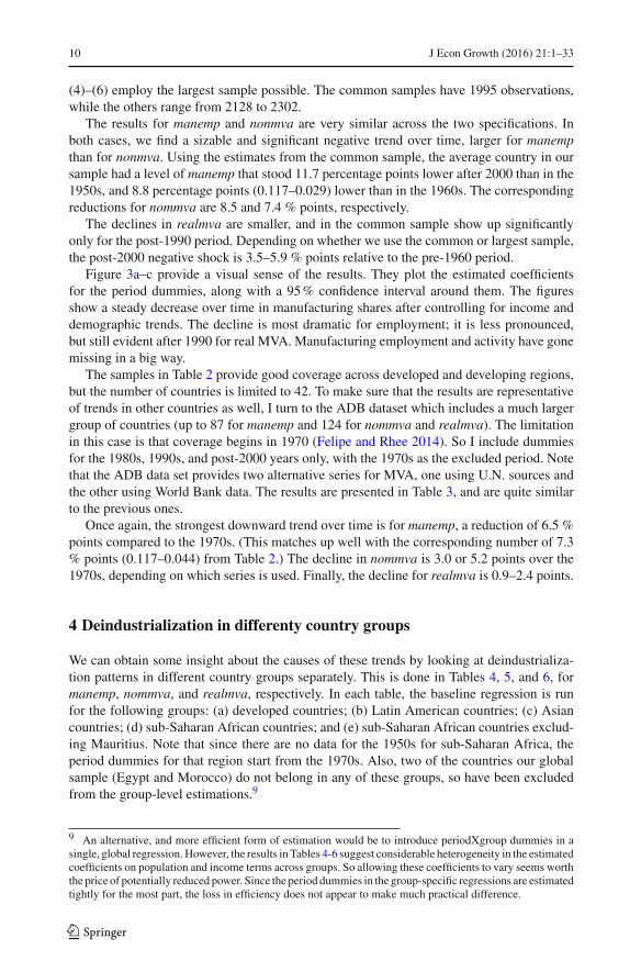
We can obtain some insight about the causes of these trends by looking at deindustrializa-tion patterns in different country groups separately. This is done in Tables 4, 5, and 6, formanemp, nommva, and realmva, respectively. In each table, the baseline regression is runfor the following groups: (a) developed countries; (b) Latin American countries; (c) Asiancountries; (d) sub-Saharan African countries; and (e) sub-Saharan African countries exclud-ing Mauritius. Note that since there are no data for the 1950s for sub-Saharan Africa, theperiod dummies for that region start from the 1970s. Also, two of the countries our globalsample (Egypt and Morocco) do not belong in any of these groups, so have been excludedfrom the group-level estimations.9

9 An alternative, and more efficient form of estimation would be to introduce periodXgroup dummies in asingle, global regression.However, the results in Tables 4-6 suggest considerable heterogeneity in the estimatedcoefficients on population and income terms across groups. So allowing these coefficients to vary seems worththe price of potentially reduced power. Since the period dummies in the group-specific regressions are estimatedtightly for the most part, the loss in efficiency does not appear to make much practical difference.

123

J Econ Growth (2016) 21:1–33 11

-0.14

-0.12

-0.1

-0.08

-0.06

-0.04

-0.02

01960s 1970s 1980s 1990s 2000+

-0.14

-0.12

-0.1

-0.08

-0.06

-0.04

-0.02

01960s 1970s 1980s 1990s 2000+

(a)

(b)

(c)

-0.14

-0.12

-0.1

-0.08

-0.06

-0.04

-0.02

01960s 1970s 1980s 1990s 2000+

Fig. 3 Estimated period coefficients (with 95% confidence intervals): a manemp b nommva c realmva

123

12 J Econ Growth (2016) 21:1–33

Table3

Alternativedatasets

manem

pnommva

realmva

ADB/ILO

ADB/UN

ADB/W

BADB/UN

ADB/W

B

lnpo

pulatio

n0.19

6∗(0.043

)0.19

4∗(0.026

)0.26

0∗(0.031

)0.00

8(0.019

)−0

.044

(0.029

)

lnpo

pulatio

nsquared

−0.004

∗ (0.00

1)−0

.004

∗ (0.00

1)−0

.007

∗ (0.00

1)0.00

1(0.001

)0.00

2∗∗ (

0.00

1)

lnGDPpercapita

0.69

3∗(0.052

)0.23

8∗(0.016

)0.14

6∗(0.019

)0.06

0∗(0.015

)0.05

7∗(0.017

)

lnGDPpercapitasquared

−0.039

∗ (0.00

3)−0

.013

∗ (0.00

1)−0

.008

∗ (0.00

1)−0

.002

∗∗(0.001

)−0

.002

∗∗∗ (

0.00

1)

1980

s−0

.023

∗ (0.00

2)−0

.011

∗ (0.00

2)−0

.002

(0.002

)−0

.006

∗ (0.00

1)0.00

0(0.002

)

1990

s−0

.043

∗ (0.00

4)−0

.029

∗ (0.00

2)−0

.010

∗ (0.00

3)−0

.016

∗ (0.00

2)−0

.003

(0.003

)

2000

s+−0

.065

∗ (0.00

5)−0

.052

∗ (0.00

3)−0

.030

∗ (0.00

4)−0

.024

∗ (0.00

3)−0

.009

∗∗(0.003

)

Country

fixed

effects

Yes

Yes

Yes

Yes

Yes

Num

berof

coun

tries

8712

411

912

411

2

Num

berof

observations

1947

4378

3691

5070

3312

Robuststandarderrorsarereported

inparentheses

Levelsof

statistiticalsignficance:∗

99%;∗

∗ 95%;∗

∗∗90

%

123

J Econ Growth (2016) 21:1–33 13

Table4

Cou

ntry

grou

ps,m

anem

p Allcountries

Developed

countries

Latin

America

Asia

Sub-SaharanAfrica

Sub-SaharanAfrica

(excl.Mauritiu

s)

lnpo

pulatio

n0.12

2∗(0.021

)−0

.652

∗ (0.12

2)0.19

1∗(0.032

)0.78

9∗(0.102

)0.19

9∗(0.019

)0.17

8∗(0.014

)

lnpo

pulatio

nsquared

−0.001

(0.001

)0.01

7∗(0.003

)−0

.003

∗ (0.00

1)−0

.025

∗ (0.00

3)−0

.005

∗ (0.00

1)−0

.004

∗ (0.00

0)

lnGDPpercapita

0.31

6∗(0.026

)1.07

0∗(0.088

)0.90

2∗(0.071

)0.91

2∗(0.071

)0.19

0∗(0.024

)0.14

8∗(0.018

)

lnGDPpercapitasquared

−0.018

∗ (0.00

2)−0

.057

∗ (0.00

5)−0

.052

∗ (0.00

4)−0

.051

∗ (0.00

4)−0

.014

∗ (0.00

2)−0

.011

∗ (0.00

1)

1960

s−0

.018

∗ (0.00

4)−0

.004

(0.004

)−0

.027

∗ (0.00

4)−0

.003

(0.013

)n.a.

n.a.

1970

s−0

.033

∗ (0.00

5)−0

.021

∗ (0.00

6)−0

.050

∗ (0.00

6)0.01

6(0.016

)0.00

2(0.004

)−0

.003

(0.003

)

1980

s−0

.054

∗ (0.00

6)−0

.052

∗ (0.00

7)−0

.079

∗ (0.00

8)0.02

2(0.019

)0.00

4(0.007

)−0

.021

∗ (0.00

5)

1990

s−0

.074

∗ (0.00

8)−0

.072

∗ (0.00

9)−0

.096

∗ (0.01

0)0.01

3(0.022

)0.00

7(0.012

)−0

.033

∗ (0.00

7)

2000

s+−0

.105

∗ (0.00

9)−0

.096

∗ (0.01

0)−0

.131

∗ (0.01

2)0.00

4(0.026

)0.00

7(0.014

)−0

.035

∗ (0.00

8)

Country

fixed

effects

Yes

Yes

Yes

Yes

Yes

Yes

Num

berof

coun

tries

4210

911

1110

Num

berof

observations

2209

575

545

519

524

481

Robuststandarderrorsarereported

inparentheses

Levelsof

statistiticalsignficance:∗

99%;∗

∗ 95%;∗

∗∗90

%

123

14 J Econ Growth (2016) 21:1–33

Table5

Cou

ntry

grou

ps,n

ommva Allcountries

Developed

countries

Latin

America

Asia

Sub-SaharanAfrica

Sub-SaharanAfrica

(excl.Mauritiu

s)

lnpo

pulatio

n0.19

2∗(0.027

)0.75

2∗∗ (

0.30

9)0.22

3∗(0.046

)1.00

9∗(0.081

)0.55

2∗(0.049

)0.51

9∗(0.045

)

lnpo

pulatio

nsquared

−0.004

∗ (0.00

1)−0

.016

∗∗(0.008

)−0

.007

∗ (0.00

1)−0

.029

∗ (0.00

2)−0

.017

∗ (0.00

1)−0

.014

∗ (0.00

1)

lnGDPpercapita

0.26

6∗(0.031

)1.02

4∗(0.139

)0.30

8∗∗∗

(0.157

)0.87

7∗(0.054

)0.04

7(0.061

)0.02

7(0.056

)

lnGDPpercapitasquared

−0.014

∗ (0.00

2)−0

.059

∗ (0.00

8)−0

.016

∗∗∗ (

0.00

9)−0

.050

∗ (0.00

3)−0

.007

(0.005

)−0

.006

(0.004

)

1960

s−0

.010

∗∗∗ (

0.00

6)−0

.003

(0.007

)−0

.001

(0.008

)0.00

8(0.007

)n.a.

n.a.

1970

s−0

.014

∗∗(0.007

)−0

.035

∗ (0.01

0)−0

.006

(0.010

)0.03

2∗(0.010

)0.03

0∗(0.005

)0.01

7∗(0.005

)

1980

s−0

.028

∗ (0.00

8)−0

.054

∗ (0.01

1)−0

.002

(0.014

)0.03

6∗(0.014

)0.02

9∗(0.008

)−0

.008

(0.009

)

1990

s−0

.049

∗ (0.00

9)−0

.062

∗ (0.01

3)−0

.010

(0.018

)0.03

3∗∗∗

(0.018

)0.01

0(0.010

)−0

.050

∗ (0.01

3)

2000

s+−0

.085

∗ (0.01

0)−0

.079

∗ (0.01

5)−0

.039

∗∗(0.020

)0.03

2(0.022

)−0

.004

(0.012

)−0

.079

∗ (0.01

6)

Country

fixed

effects

Yes

Yes

Yes

Yes

Yes

Yes

Num

berof

coun

tries

4210

911

1110

Num

berof

observations

2128

451

498

576

565

512

Robuststandarderrorsarereported

inparentheses

Levelsof

statistiticalsignficance:∗

99%;∗

∗ 95%;∗

∗∗90

%

123

J Econ Growth (2016) 21:1–33 15

Table6

Cou

ntry

grou

ps,realmva Allcountries

Developed

countries

Latin

America

Asia

Sub-SaharanAfirca

Sub-SaharanAfirca

(excl.Mauritiu

s)

lnpo

pulatio

n−0

.039

(0.025

)−4

.564

∗ (0.77

6)0.26

3∗(0.027

)0.25

1∗(0.084

)0.06

2∗∗ (

0.02

9)0.05

3∗∗∗

(0.031

)

lnpo

pulatio

nsquared

0.00

3∗(0.001

)0.11

3∗(0.019

)−0

.004

∗ (0.00

1)−0

.011

∗ (0.00

3)−0

.001

(0.001

)−0

.000

(0.001

)

lnGDPpercapita

0.26

2∗(0.027

)0.77

8∗(0.129

)−0

.135

∗∗(0.059

)0.73

7∗(0.040

)0.12

3∗(0.025

)0.10

6∗(0.024

)

lnGDPpercapitasquared

−0.012

∗ (0.00

2)−0

.036

∗ (0.00

8)0.00

6∗∗∗

(0.003

)−0

.038

∗ (0.00

3)−0

.009

∗ (0.00

2)−0

.008

∗ (0.00

2)

1960

s−0

.028

∗ (0.00

7)−0

.021

∗∗∗ (

0.01

1)−0

.011

∗ (0.00

4)0.01

1∗∗∗

(0.006

)n.a.

n.a.

1970

s−0

.026

∗ (0.00

8)0.00

7(0.015

)−0

.017

∗ (0.00

6)0.02

7∗(0.010

)0.01

7∗(0.005

)0.01

2∗(0.004

)

1980

s−0

.034

∗ (0.00

9)0.00

6(0.018

)−0

.052

∗ (0.00

7)0.03

4∗∗ (

0.01

3)0.01

5∗∗ (

0.00

6)−0

.004

(0.006

)

1990

s−0

.040

∗ (0.01

0)0.01

3(0.023

)−0

.078

∗ (0.00

8)0.04

1∗∗ (

0.01

7)0.01

1(0.009

)−0

.022

∗ (0.00

8)

2000

s+−0

.059

∗ (0.01

1)0.02

1(0.027

)−0

.101

∗ (0.01

0)0.04

4∗∗ (

0.02

0)−0

.003

(0.011

)−0

.042

∗ (0.01

0)

Country

fixed

effects

Yes

Yes

Yes

Yes

Yes

Yes

Num

berof

coun

tries

4210

911

1110

Num

berof

observations

2302

592

556

577

530

487

Robuststandarderrorsarereported

inparentheses

Levelsof

statistiticalsignficance:∗

99%;∗

∗ 95%;∗

∗∗90

%

123

16 J Econ Growth (2016) 21:1–33

The results point to important regional differences. First, even though developed countrieshave experienced big losses in manemp and nommva, they have done surprisingly well inrealmva. The estimated coefficients for the period dummies for realmva are in fact positive(but statistically insignificant) for the developed countries in recent decades (Table 6). This isto be compared with significant negative estimates for Latin America and Africa (once Mau-ritius is excluded). To be clear, this does not mean that the rich nations have not experiencedreductions in real manufacturing output shares in GDP. It simply means that their experiencecan be well explained by income and demographic trends, with little unexplained (output)deindustrialization left to account for in recent decades.

The results for Asia are even more striking. Asia is the only region for which recent perioddummies are not negative for manemp (once again, if Mauritius is excluded from the sub-Saharan sample). And the estimates for realmva in recent periods are actually positive andstatistically significant. These results suggest that Asia has not only bucked the global trend inmanufacturing employment, it hasmanaged tomaintain strongermanufacturing performancethan would be expected on the basis of its income and demography.

The region that has done the worst is Latin America, which has the most negative recent-period effects for manemp and realmva. The effects for nommva are not as pronounced,suggesting that relative prices have not moved there against manufacturing nearly as muchas in other regions. Finally, the estimates for sub-Saharan Africa depend heavily on whetherMauritius – a strongmanufactures exporter – is included in the sample or not.WithoutMauri-tius in the sample, sub-Saharan African countries emerge as large losers on all three measuresof industrialization. Their output deindustrialization in recent decades looks especially dra-matic in light of the strong showing for realmva in the 1970s (captured by a positive andsignificant coefficient for dum1970s in Table 6). Since sub-Saharan countries are still verypoor and widely regarded as the next frontier of labor-intensive export-oriented manufactur-ing, these are quite striking findings.

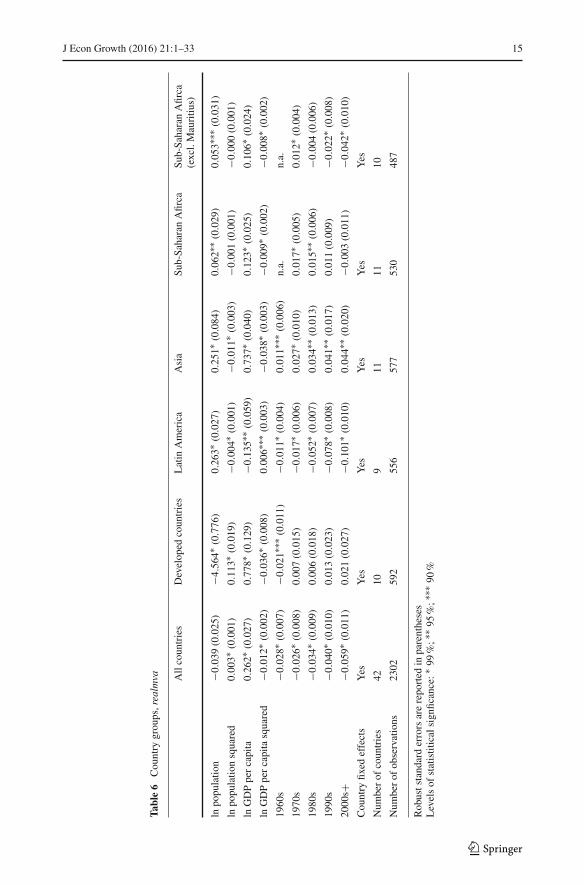
The results with respect to Asia and the difference that the inclusion of Mauritius makesto the African performance strongly suggests that these variations in outcomes are relatedto patterns of comparative advantage, and, in particular, how well or poorly countries havedone in global trade in manufactures. To test this idea, I divide our sample of countriesinto two groups: (a) manufactures exporters, and (b) non-manufactures exporters. I use twocriteria to split the sample based on the composition of trade. The first classifies countries asmanufactures exporters if the share of manufactures in exports exceeds 75 %, the second ifthe share of manufactures in exports exceeds the corresponding share in imports.

The results, shown in Table 7, support the comparative-advantage hypothesis. Regardlessof the criterion used, the employment loss in manufactures exporters is smaller. Whereasthe period effects for realmva are strongly negative and significant for manufactures non-exporters, they change sign and are occasionally significant for manufactures exporters.Regressions using ADB data, with broader country coverage, produce very similar results(Table 8). The period effects for manemp are not distinguishable between the two groupswith this sample, but the realmva results show even stronger asymmetries.

In sum, the geographical patterns of deindustrialization seem closely linked to globaliza-tion. Our results apparently reflect the sizable shift in global manufacturing activity in recentdecades towards East Asia, and China in particular, with both Latin America and sub-SaharanAfrica among the developing regions as the losers (see Table 1). Countries with a strong com-parative advantage in manufactures have managed to avoid declines in real MVA shares, andemployment losses, where they have occurred, have been less severe. Interestingly, on theoutput side it appears that the brunt of globalization and the rise of Asian exporters has beenborne by other developing countries, rather than the advanced economies. What is partic-

123

J Econ Growth (2016) 21:1–33 17

Table7

Resultsby

manufacturing

specialization

Non-m

anufacturesexporters

Manufacturesexporters

Manufactured

exports<

75%

Shareof

manufacturedexpo

rts

<shareof

manufactured

imports

Manufactured

exports>

75%

Shareof

manufacturedexpo

rts

>shareof

manufactured

impo

rts

manem

prealmva

manem

prealmva

manem

prealmva

manem

prealmva

lnpo

pulatio

n0.202∗

(0.025)

0.146∗

(0.031)

0.174∗

(0.028)

0.130∗

(0.031)

0.326∗

(0.035)

0.034(0.034)

0.444∗

(0.025)

0.184∗

(0.033)

lnpo

pulatio

nsquared

−0.003

∗(0.001)

−0.001

∗∗∗(0.001)

−0.002

∗∗(0.001)

−0.001

(0.001)

−0.009

∗(0.001)

−0.002

∗∗(0.001)

−0.014

∗(0.001)

−0.007

∗(0.001)

lnGDPpercapita

0.172∗

(0.021)

0.314∗

(0.051)

0.161∗

(0.022)

0.314∗

(0.051)

0.704∗

(0.043)

0.645∗

(0.021)

0.772∗

(0.042)

0.627∗

(0.025)

lnGDPpercapita

squared

−0.010

∗(0.001)

−0.018

∗(0.003)

−0.009

∗(0.001)

−0.017

∗(0.003)

−0.039

∗(0.003)

−0.033

∗(0.001)

−0.042

∗(0.003)

−0.032

∗(0.002)

1960s

−0.032

∗(0.004)

−0.055

∗(0.011)

−0.028

∗(0.004)

−0.057

∗(0.011)

−0.004

(0.006)

0.004(0.003)

−0.002

(0.005)

0.007∗

∗∗(0.004)

1970s

−0.057

∗(0.005)

−0.070

∗(0.013)

−0.054

∗(0.005)

−0.073

∗(0.013)

−0.004

(0.008)

0.024∗

(0.005)

−0.002

(0.008)

0.030∗

(0.005)

1980s

−0.080

∗(0.006)

−0.087

∗(0.015)

−0.078

∗(0.006)

−0.091

∗(0.015)

−0.025

∗(0.009)

0.014∗

∗(0.007)

−0.020

∗∗(0.009)

0.022∗

(0.007)

1990s

−0.093

∗(0.007)

−0.097

∗(0.016)

−0.093

∗(0.008)

−0.101

∗(0.017)

−0.057

∗(0.011)

0.013(0.008)

−0.050

∗(0.011)

0.019∗

∗(0.009)

2000

s+−0

.120

∗(0.009)

−0.123

∗(0.018)

−0.123

∗(0.009)

−0.128

∗(0.019)

−0.089

∗(0.013)

0.012(0.010)

−0.079

∗(0.013)

0.014(0.011)

Cou

ntry

fixed

effects

Yes

Yes

Yes

Yes

Yes

Yes

Yes

Yes

Num

berof

coun

tries

2626

2626

1616

1616

Num

berof

observations

1366

1426

1378

1425

843

876

831

877

Robuststandarderrorsarereported

inparentheses

Levelsof

statistiticalsignficance:∗

99%;∗

∗ 95%;∗

∗∗90

%

123

18 J Econ Growth (2016) 21:1–33

Table8

Resultsby

manufacturing

specialization(A

DB/ILO/W

Bdata)

Non-m

anufacturesexporters

Manufacturesexporters

Manufactured

exports<

75%

Shareof

manufacturedexpo

rts<

shareof

manufacturedim

ports

Manufactured

exports>

75%

Shareof

manufacturedexpo

rts>

shareof

manufacturedim

ports

manem

prealmva

manem

prealmva

manem

prealmva

manem

prealmva

lnpo

pulatio

n0.130∗

(0.049)

−0.094

∗∗(0.040)

0.130∗

(0.046)

−0.131

∗(0.050)

−0.036

(0.130)

0.132∗

∗(0.053)

0.022(0.1135)

0.116∗

(0.043)

lnpo

pulatio

nsquared

−0.002

(0.002)

0.004∗

(0.001)

−0.002

(0.002)

0.006∗

(0.002)

0.001(0.004)

−0.005

∗(0.002)

−0.001

(0.003)

−0.004

∗(0.001)

lnGDPpercapita

0.525∗

(0.056)

0.065∗

(0.017)

0.528∗

(0.061)

0.078∗

(0.018)

0.825∗

(0.008)

0.173∗

(0.032)

0.817∗

(0.069)

0.102∗

(0.031)

lnGDPpercapita

squared

−0.030

∗(0.003)

−0.003

∗(0.001)

−0.030

∗(0.003)

−0.004

∗(0.001)

−0.045

∗(0.0

05)

−0.008

∗(0.002)

−0.045

∗(0.004)

−0.003

(0.002)

1980s

−0.028

∗(0.003)

−0.008

∗(0.002)

−0.028

∗(0.003)

−0.007

∗(0.003)

−0.018

∗(0.003)

0.018∗

(0.003)

−0.019

∗(0.003)

0.010∗

(0.003)

1990s

−0.042

∗(0.004)

−0.016

∗(0.003)

−0.042

∗(0.004)

−0.013

∗(0.003)

−0.049

∗(0.005)

0.023∗

(0.005)

−0.049

∗(0.004)

0.009∗

∗(0.004)

2000

s+−0

.066

∗(0.006)

−0.028

∗(0.004)

−0.066

∗(0.006)

−0.026

∗(0.0049)

−0.069

∗(0.007)

0.034∗

(0.006)

−0.071

∗(0.006)

0.015∗

(0.006)

Cou

ntry

fixed

effects

Yes

Yes

Yes

Yes

Yes

Yes

Yes

Yes

Num

berof

coun

tries

5580

5273

3232

3539

Num

berof

observations

1058

2411

1028

2238

889

901

919

1074

Robuststandarderrorsarereported

inparentheses

Levelsof

statistiticalsignficance:∗

99%;∗

∗ 95%;∗

∗∗90

%

123

J Econ Growth (2016) 21:1–33 19

ularly striking is the magnitude of adverse employment effects in Latin America, which iseven larger than in developed economies.

5 Employment deindustrialization by skill groups

As the results abovemake clear, deindustrialization shows upmost clearly and in its strongestform in employment. The only countries that have managed to avoid a steady decline inmanufacturing employment in recent decades (as a share of total employment) are thosewith a strong comparative advantage in manufacturing. The Socio Economic Accounts ofthe World Input-Output Database (WIOD, Timmer 2012) allow us to dig a bit deeper onthe employment impacts. These data provide a breakdown of manufacturing employment bythree worker types: low-skill, medium-skill, and high-skill. The data span the years 1995–2009 and include 40 countries, with the coverage biased heavily towards Europe. (For thelist of countries included see the Appendix.)

I run essentially the same regression as before, with two differences. First, the dependentvariable is manufacturing’s share of the economy’s total employment of workers of a par-ticular skill type. Second, since the data start from 1995, I use annual dummies rather thandecade dummies. (As before, there is a full set of country fixed effects.) This gives us threeregressions, one for each skill type.

Figure 4 plots the estimated coefficients for the year dummies. The results are quitestriking, in that virtually the entire reduction over time in employment comes in the low-skillcategory. Manufacturing’s share of low-skill employment has come down by 4 percentagepoints between 1995 and 2009, a decline that is statistically highly significant. The decline inmedium-skill employment is miniscule by comparison, while manufacturing’s share of high-

-0.045

-0.04

-0.035

-0.03

-0.025

-0.02

-0.015

-0.01

-0.005

0

0.005

1996 1997 1998 1999 2000 2001 2002 2003 2004 2005 2006 2007 2008 2009

low-skill employment

intermediate-skill employment

high-skill employment

Fig. 4 Estimated year coefficients for employment of different skill types

123

20 J Econ Growth (2016) 21:1–33

ITA 1980

GBR 1961

USA 1953NLD 1964

SWE 1961

DNK 1962JPN 1969

FRA 1974

KOR 1989

ESP 1975

GHA 1978

MUS 1990

NGA 1982

ZAF 1981

ZMB 1985

ARG 1958

BRA 1986

CHL 1954

COL 1970

CRI 1992

IDN 2001IND 2002

MEX 1980

MYS 1997

PER 1971

0.1

.2.3

.4

6 7 8 9 10

peak manufacturing employment share Fitted values

Fig. 5 Income at which manufacturing employment peaks (logs)

skill employment has actually slightly increased over the same period. The chart underscoresin a dramatic fashion that it is low-skill workers who have borne the lion’s share of the impactof recent changes in trade and technology on manufacturing.

6 Premature deindustrialization

Our results so far suggest that late industrializers will reach peak levels of industrialization, asmeasured bymanemp and realmva, that are quite a bit lower than those experienced by earlyindustrializers. Let us denote these peak levels bymanemp* and realmva*. There is evidencethat suggests these peak levels are reached at lower levels of income as well. Denote that levelof income by y∗. Our baseline regressions capture the downward shift in the manufacturinghump over time, but not the possibility that the curve may be moving closer to the origin aswell.

Figure 5 suggests that manemp∗ and y∗ are in fact both lower for more recent indus-trializers. The figure displays manemp and y levels for the years of peak employmentindustrialization. (I have determined the turnaround years by looking at each country indi-vidually and identifying visually the year at which manemp begins to decline.) Compare thetwo sets of countries at the opposite ends of the chart. Industrialization peaked in WesternEuropean countries such as Britain, Sweden, and Italy at income levels of around $14,000(in 1990 dollars). India and many sub-Saharan African countries appear to have reached theirpeak manufacturing employment shares at income levels of $700.10

Figure 5 represents a heuristic exercise that does not permit statistical testing. To checkmore systematically how the industrialization inverse U-curve has shifted over time, I run

10 For a similar chart, see Felipe and Rhee 2014.

123

J Econ Growth (2016) 21:1–33 21

Table 9 Regressions with interaction terms for post-1990

manemp realmava

ln population 0.166∗ (0.019) −0.016 (0.025)

ln population squared −0.005∗ (0.001) 0.001 (0.001)

ln GDP per capita 0.326∗ (0.018) 0.273∗ (0.029)

ln GDP per capita squared −0.018∗ (0.001) −0.013∗ (0.002)

ln GDP per capita X post-1990 0.031∗ (0.002) 0.015∗ (0.002)

ln GDP per capita squared X post-1990 −0.004∗ (0.000) −0.002∗ (0.000)

Country fixed effects Yes Yes

Number of countries 42 42

number of observations 2209 2302

Robust standard errors are reported in parenthesesLevels of statistitical signficance: ∗ 99%; ∗∗ 95%; ∗∗∗ 90%

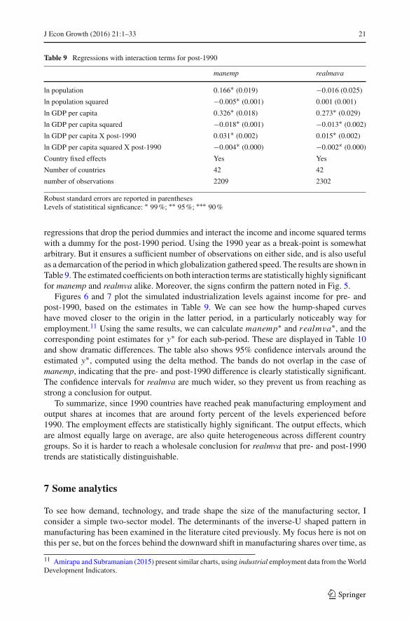
regressions that drop the period dummies and interact the income and income squared termswith a dummy for the post-1990 period. Using the 1990 year as a break-point is somewhatarbitrary. But it ensures a sufficient number of observations on either side, and is also usefulas a demarcation of the period inwhich globalization gathered speed. The results are shown inTable 9. The estimated coefficients on both interaction terms are statistically highly significantfor manemp and realmva alike. Moreover, the signs confirm the pattern noted in Fig. 5.

Figures 6 and 7 plot the simulated industrialization levels against income for pre- andpost-1990, based on the estimates in Table 9. We can see how the hump-shaped curveshave moved closer to the origin in the latter period, in a particularly noticeably way foremployment.11 Using the same results, we can calculate manemp∗ and realmva∗, and thecorresponding point estimates for y∗ for each sub-period. These are displayed in Table 10and show dramatic differences. The table also shows 95% confidence intervals around theestimated y∗, computed using the delta method. The bands do not overlap in the case ofmanemp, indicating that the pre- and post-1990 difference is clearly statistically significant.The confidence intervals for realmva are much wider, so they prevent us from reaching asstrong a conclusion for output.

To summarize, since 1990 countries have reached peak manufacturing employment andoutput shares at incomes that are around forty percent of the levels experienced before1990. The employment effects are statistically highly significant. The output effects, whichare almost equally large on average, are also quite heterogeneous across different countrygroups. So it is harder to reach a wholesale conclusion for realmva that pre- and post-1990trends are statistically distinguishable.

7 Some analytics

To see how demand, technology, and trade shape the size of the manufacturing sector, Iconsider a simple two-sector model. The determinants of the inverse-U shaped pattern inmanufacturing has been examined in the literature cited previously. My focus here is not onthis per se, but on the forces behind the downward shift in manufacturing shares over time, as

11 Amirapu and Subramanian (2015) present similar charts, using industrial employment data from theWorldDevelopment Indicators.

123

22 J Econ Growth (2016) 21:1–33

0

0.05

0.1

0.15

0.2

0.25

6 6.26.46.66.87 7.27.47.67.88 8.28.48.68.89 9.29.49.69.810 10.210.410.610.811 11.211.411.611.812

pre-1990

post-1990

ln 1990 US $

Fig. 6 Simulated manufacturing employment shares

-0.05

0

0.05

0.1

0.15

0.2

0.25

0.3

6 6.26.46.66.87 7.27.47.67.88 8.28.48.68.89 9.29.49.69.810 10.210.410.610.811 11.211.411.611.812

pre-1990

post-1990

ln 1990 US $

Fig. 7 Simulated manufacturing output shares (MVA/GDP at constant prices)

123

J Econ Growth (2016) 21:1–33 23

Table 10 Maximum industrialization levels, pre- and post-1990

manemp realmva

Pre-1990 Post-1990 Pre-1990 Post-1990

Maximum share 21.5% 18.9% 27.9% 24.1%

Reached at income level(GDP per capita, in 1990international )$

$ 11,048 $ 4273 $ 47,099 $ 20,537

95% confidence interval [8785, 14,017] [3831, 4735] [19,667, 112,081] [12,429, 34,061]

Source: Author’s calculations; see text

documented previously. The model is barebones, and I claim no novelty for it. For the mostpart, it summarizes existing results in the literature. The framework’s main advantage is thatit looks at the effects of different types of shocks on both employment- and output-basedmeasures of industrialization. For more complete formal treatments of structural change, seeMatsuyama (1992 and 2009), Ngai and Pissarides (2004), Buera and Joseph (2009), Foellmiand Zweimuller (2008), and Nickell et al. (2008).12

Let the economy be divided into manufacturing (m) and non-manufacturing (n), with aconstant labor force fixed at unity. The share of employment in the manufacturing sector(manemp) is denoted by α. Production functions in the two sectors exhibits diminishingmarginal returns to labor and are written as follows:

qsm = θmαβm (1)

qsn = θn(1 − α)βn , (2)

where qsm and qsn are the quantities supplied of manufactures and non-manufactures, respec-tively, θm and θn are parameters capturing the productivity of the two sectors, and βm andβn are technological constants between 0 and 1. The results in Sect. 5 provide strong hintsof technological bias away from unskilled labor. But my focus here is on changes in theoverall labor requirements in manufacturing rather than on substitution among different skillcategories. The former is appropriately captured by shifts in the parameter θm .

It is convenient to represent the demand side in rates of change form, with a “hat” abovea variable denoting proportional changes (y = dy/y):

qdm − qdn = −σ(pm − pn

), (3)

where σ is the elasticity of substitution in consumption between the two goods. There aretwo goods-market clearing equations:

qdm + x = qsm (4)

qdn = qsn, (5)

where x stands for the net exports of the manufactured good. (For simplicity, I assumebalanced trade in non-manufactures.) Labor is fully employed and mobile between the two

12 For models of industrialization with increasing returns and inter-industry linkages, see also Rodríguez-Clare (1996), Venables (1996), and Rodrik (1996).

123

24 J Econ Growth (2016) 21:1–33

sectors. This gives us our final equation, which is the labor-market equilibrium equation:

βm pmθmαβm−1 = βn pnθn (1 − α)βn−1 (6)

This equation equates the value marginal product of labor in the two sectors.Since we can only determine relative prices, let’s take the non-manufactured good

to be the numeraire, fixing pn at unity. We are left with seven endogenous variables:α, qdn , qsn, q

dm, qsm, pm and x . We would need an additional, global market-clearing equa-

tion to determine pm and x simultaneously. This in turn requires modeling the rest of theworld as well. Here I will take a short-cut and make one of two extreme assumptions. Inone case, prices are determined endogenously by developments in the home economy andnet trade flows are exogenous. In the second case, the economy is sufficiently small that itremains a price taker in world markets (so that x is endogenous and pm is a parameter).13

These two characterizations are meant to capture the situations in the large developed andthe developing countries, respectively.

Consider first the advanced economy case. Doing the comparative statics for the employ-ment share of manufacturing, we get

dα = ψ

[(σ − λ

σ

)θm −

(σ − 1

σ

)θn + 1

σ

dx

qdm

], (7)

where

ψ =[1

α(1 − βm) + 1

1 − α(1 − βn) + 1

σ

(λ

αβm + 1

1 − αβn

)]−1

> 0

and

λ = qsmqdm

.

A lower trade surplus, or bigger trade deficit, in manufacturing (dx < 0) results in a smalleremployment share in manufacturing, which is not surprising. Note that a reduction in x isformally analogous to an adverse demand shock for manufactures, such as a secular shiftin demand towards services and other non-manufactures. In both cases, the manufacturingsector shrinks.

The relationship between technological progress (θm, θn) andα, on the other hand, dependscritically on the size of the elasticity of substitution in demand between manufactures andnon-manufactures. Suppose for the moment that net trade in manufactures is small so thatλ ≈ 1. Then if demand is inelastic (σ < 1), α is decreasing in technological progressin manufactures (θm) and increasing in technological progress in non-manufactures (θn).More rapid TFP growth in manufacturing, which is the usual case, results in employmentdeindustrialization. Intuitively, the technological progress-induced reduction in the relativeprice of manufacturing does not spur demand for manufactures sufficiently, so that the netresult is a squeeze in manufactures employment. These results are reversed when demand iselastic (σ > 1). This is the same as the finding in Ngai and Pissarides (2004).14

13 I assume that manufactures are the only goods that are traded. In reality, many services are also traded,and the share that crosses national borders has increased over time. Still, even though services dominate thedomestic economy, they amount to less than a quarter of global trade. For measurement and other issues posedby trade in services, see World Trade Organization (WTO 2010).14 Baumol and Bowen (1965) and Baumol (1967) are the classic works that looked at the consequences oflower productivity growth in services relative to manufactures.

123

J Econ Growth (2016) 21:1–33 25

The effect of technological progress in manufacturing, however, is also mediated throughλ, the ratio of supply to demand in manufacturing. This is something that has not beenemphasized in the earlier literature, which typically assumes a closed economy. Consider thecase where a country is a large net importer of manufactures (λ � 1). As can be seen from(7), as long as σ − λ > 0 the coefficient that multiplies θm is positive. This is possible evenwhen σ < 1 and demand for manufactures is inelastic. So we have a reversal of the result thatinelastic demand and rapid technological progress in manufacturing produce (employment)deindustrialization.

The intuition behind this is as follows. The lower the share of domestic supply in totalconsumption, the smaller the effect of TFP in domestic manufactures on relative prices.When manufacturing experiences rapid productivity growth, it experiences less decline inrelative prices (compared to a country where domestic supply is a large share of domesticconsumption). Consequently, domestic output and employment are larger in equilibrium. Inthe limit, when technological progress has no effect on domestic relative prices, manufactur-ing employment is always boosted by TFP growth in manufactures. This is indeed the casein our other benchmark example, a small open economy which takes its relative prices fromworld markets.

Before we turn to that case, however, let us also look at the output share of manufac-turing and how it is affected by trade and technology. Denote the real value added share ofmanufacturing (realmva) by αq :

αq = qsmqsm + qsn

.

We can now relate output-deindustrialization (dαq) to employment deindustrialization (dα)

as follows:

dαq = αq(1 − αq

) [θm − θn +

(1

αβm + 1

1 − αβn

)dα

]. (8)

This shows that when the main shock comes from trade or demand (with θm = θn = 0), thetwomeasures of industrialization always move in the sameway. However, when employmentdeindustrialization is due to differential TFP growth in manufacturing (θm − θn > 0), it ispossible for the output share of manufacturing to move very little, or even to increase.

To see this in greater detail, consider the case where the economy does not trade atall so that λ = 1. In this case, the output share of manufacturing must in fact rise. Wecan read this off readily from the demand-side relationship (3). Differential productivitygrowth in manufacturing depresses the relative price of manufacturing, and this impliesqdm = qsm > qdn = qsn , and therefore dαq > 0. Or, substituting (7) into (8) and solving, weget:

dαq = αq(1 − αq

)⎧⎨

⎩

(σ

σ−1

)

(σ

σ−1

)− [(1 − α) βm + αβn]

⎫⎬

⎭

(θm − θn

).

Since the term in curly brackets is positivewhen σ < 1,αq mustmove in the same direction asdifferential productivity growth in manufacturing. This establishes that in an economy wheretrade plays a small role, rapid technological progress in manufacturing produces employmentdeindustrialization, but not output deindustrialization.

123

26 J Econ Growth (2016) 21:1–33

Let us look now at the small-open economy case. For this case, we treat price changesparametrically and take x to be endogenous. The comparative statics yields:

dα =[1

α(1 − βm) + 1

1 − α(1 − βn)

]−1 [pm + θm − θn

]. (9)

Technological progress in manufacturing now has an unambiguously positive effect on α.

Technological progress in non-manufacturing has an unambiguously negative effect. Andan increase in the relative price of manufacturing works just like technological progressin manufacturing. Moreover, the result does not depend on σ or its magnitude, as tradehas the effect of de-linking the supply side of the economy from the demand side. For thesame reason, adverse domestic demand shocks would not produce deindustrialization inthe small open economy; domestic producers can sell the surplus output on world markets.As Matsuyama (2009) has previously emphasized, the relationship between productivitygrowth and industrialization depends crucially on whether we treat prices to be determineddomestically or in the global economy.15

This last set of results is important in interpreting the experience of developing countriesthat have experienced rapid deindustrialization. These countries tend to be small in globalmarkets formanufacturing, sowe can take treat them as price takers.What equation (9) showsis that employment deindustrialization in those countries cannot have been the consequence ofdifferentially rapidTFPgrowth inmanufacturing at home.That kind of technological progresswould have fostered industrialization, rather than the reverse. In this respect, developingcountries are quite different from the advanced countrieswhere there is considerable evidencethat domestic technological progress was the culprit.

As price takers, however, these developing countries may have “imported” deindustri-alization from the abroad. Most countries in Latin America undertook significant tradeliberalizations in the second half of the 1980s and early 1990s, transforming themselvesinto open economies. Many countries in Sub-Saharan Africa experienced trade opening aswell around the same time. As (9) shows, a decline in the relative price of manufactures( pm < 0) – the result of technological progress elsewhere, the rise of China, domestictrade liberalization, or all three – would have had the same effect as technological regress athome in manufacturing. Even with more rapid TFP growth in manufacturing (compared tonon-manufacturing), these countries would find themselves deindustrializing in employmentterms.

Putting it differently, employment industrialization in the developing world requires morethan differentially rapid TFP growth inmanufacturing. It requires that the productivity growthdifferential between manufacturing and non-manufacturing also exceed the decline in man-ufactures’ relative prices on world markets. Our empirical results suggest that only very fewdeveloping countries managed this feat consistently.

The configuration of analytical results under different assumptions about economic closureand the nature of the shocks is summarized in the table below.

15 Matsuyama (2009) shows that cross-country results have to be interpreted with caution when economiesare globally integrated. In particular, faster productivity gains need not be correlated with more rapid declinein manufacturing across countries, even if productivity change is globally responsible for manufacturing’sdecline. See also Uy et al. (2013) which develops a model with productivity and trade cost shocks undervarious assumptions about demand, and uses it to explain South Korea’s pattern of structural change. Theauthors find that non-homothetic demand, more rapid productivity growth in manufacturing, and the declinein manufacturing trade costs do a good job of explaining structural change, with the exception of the declinein manufacturing after 1990.

123

J Econ Growth (2016) 21:1–33 27

Effects of trade, technology, and demand on different measures of industrialization

A. “Closed” economy (with σ < 1)

Effect on: Technology shock:θm − θn > 0

Trade shock: dx < 0 Adverse domesticdemand shock onmanufacturing

manemp (dα) − − −realmva (dαq ) + − −B. Small open economy

Effect on: Technology shock:θm − θn > 0

External price shock:pm < 0

Adverse domesticdemand shock onmanufacturing

manemp (dα) + − 0realmva (dαq ) + − 0

These are all ceteris paribus results, for the case where each country can be treated indi-vidually. We need to exercise care in interpreting them when technology (or demand) shocksoccur in many countries simultaneously (requiring us to explicitly endogenize trade vol-umes and relative prices on world markets). Consider the consequences of technologicalprogress in manufacturing that takes place in both developed and developing countries. Aslong as the (global) supply ofmanufactures exceeds supply of non-manufactures at unchangedprices, the consequence is that pm < 0 for all countries. Those countries which have expe-rienced less technological progress in manufacturing will see their manufacturing industriessuffer declines in output, even though productivity has increased. When TFP growth inmanufacturing is global, only those countries with the more rapid TFP growth will avoiddeindustrialization. So for Latin America or Africa to experience industrialization as openeconomies, they must have had TFP growth in manufacturing that was faster than in the restof the world, which evidently did not happen.

Finally, we can use this framework also to interpret the consequences of resource rents andrelated Dutch-disease issues in open economies.Many Latin American andAfrican countrieshave experienced booming primary sectors as a consequence of resource discoveries and a risein commodity price. In the presentmodel a resource boomwouldmanifest itself as an increasein productivity growth and/or prices in non-manufacturing (relative to manufacturing, in bothcases). The effects for small open economies can be read off the first two columns in partB of the table above: the economy suffers both employment and output deindustrialization.Effectively, resource booms magnify the deindustrializing consequences that trade has oncountries with comparative advantage in primary products.16

8 Concluding remarks: implications and consequences

One way to understand the transformation in global manufacturing documented here is toconsider the analogy of a closed economy with three regions: a high-income region that isalready industrialized, and two low-income regions, onewith a strong comparative advantage

16 Aid inflows operate similarly to resource booms in so far as they drive up the price of non-traded goods,and reduce the relative price of manufactures. For an examination of these issues in the Sub-Saharan Africanand Latin American contexts, respectively, see Rajan and Subramanian (2011) and Palma (2014).

123

28 J Econ Growth (2016) 21:1–33

(or head start) in manufacturing and the other without.17 The economy experiences twoshocks: (low-skill) labor-saving technological progress and decline in transport/transactioncosts among regions. We would then observe the following patterns: (i) a sharp decline inmanufacturing employment in the high-income region, with the impact on manufacturingoutput (at constant prices) depending on the balance between technology (positive) and trade(negative) shocks; (ii) an increase in output and (possibly) employment in the low-incomeregion with the comparative advantage (or head start) in manufactures; and (iii) a decline inboth output and employment in the other low-income region. These consequences broadlycapture the trends we have seen in the advanced economies, Asian manufactures exporters,and other developing economies, respectively.

How concerned should low- and middle-income countries be about their “premature” de-industrialization? The previous section treated productivity growth as exogenous, to examineits consequences for industrialization under different economic structures. But there is areverse channel of causation as well, especially in developing countries, which goes fromindustrialization to economy-wide productivity. In low-income settings, the movement ofworkers from the countryside to urban factories where their productivity tends to be muchhigher is an important source of productivity growth. Industrialization contributes to growthboth because of this reallocation effect and because manufacturing tends to experience rel-atively stronger productivity growth over the medium to longer term. In fact, organized,formal manufacturing appears to exhibit unconditional convergence, which makes it a potentengine of growth (Rodrik 2013, 2014).18 From this perspective, premature deindustrializa-tion is not good news for developing nations. It blocks off the main avenue of rapid economicconvergence in low-income settings.19

The consequences are already visible in the developing world. In Latin America, as man-ufacturing has shrunk informality has grown and economy-wide productivity has suffered.In Africa, urban migrants are crowding into petty services instead of manufacturing, anddespite growing Chinese investment there are as yet few signs of a significant resurgence inindustry. McMillan and Rodrik (2011) analyze employment patterns in a broad cross-section

17 I am grateful to an anonymous referee who suggested the closed-economy analogy.18 Young (November 2013 and forthcoming) raises some important questions about gaps in inter-sectoralproductivity and in manufacturing versus nonmanufacturing productivity growth, arguing that these gaps maybe due to selection based on unobserved worker skills. To the extent that manufacturing is more productivebecause it employs the more capable workers, it loses its “specialness.” In particular, more labor absorptionin manufacturing would not raise economy-wide productivity, as marginal workers drawn into manufacturingwould be of the lower-productivity type. Even if selection effects are present, however, it is not clear theycan explain why manufacturing industries that are further away from the frontier experience more rapidlabor productivity growth (as in Rodrik 2013). A recent paper by Franck and Galor (2015) suggests earlyindustrialization may have adverse long-run effects, within a country: these authors find that regions in Francethat adopted industrial technology earlier eventually ended up with lower incomes and human capital levels.It is not clear what the implications of such results to growth patterns across countries are, however. France isa post-industrial country, and the cross-region findings are conditional on industrialization and within-countryconvergence having taken place.19 A full welfare evaluation of the trends discussed in this paper must take into account other effects inaddition to the foregone productivity gains due to premature deindustrialization. For developing countriesthat are net importers of manufactures, the global reduction in the relative price of manufactures due totechnological progress in advanced countries represents a terms-of-trade benefit and a (static) welfare gain.(For developing countries that are net exporters of manufactures, there is a corresponding terms-of-trade loss.)The fall in manufacturing prices may also reduce the cost of capital-goods in developing countries, and therebyspur investment. Where private investment is sub-optimal due to credit-market or other failures, this wouldrepresent an additional source of welfare gain. It is in principle possible to attach some quantitative magnitudesfor representative countries to each one of these effects, using the results here and in Rodrik (2013). However,such an effort would take this paper too far afield, and I leave it to future work.

123

J Econ Growth (2016) 21:1–33 29

of developing economies and find that labor has been moving in the wrong direction in LatinAmerica and Africa – to low productivity services and away from high productivity activitiessuch as manufacturing. So structural change has ended up being growth-reducing in thesecountries in recent decades, unlike the 1950-75 period during which it made a strong positivecontribution to growth (see also de Vries et al. 2013, and McMillan et al. 2014).20

There has been no lack of growth in the developing world since the mid-1990s. Butoutside of Asia and the small group of manufactures exporters, the evidence (cited in theprevious paragraph) shows that this growth has not been driven by the traditional mechanismof industrialization.Many of the growth booms appear to have been driven by capital inflows,external transfers, or commodity booms, raising questions about their sustainability.21

In the absence of sizable manufacturing industries, these economies will need to dis-cover new growth models. One possibility is services-led growth. Many services, such as ITand finance, are high productivity and tradable, and could play the escalator role that man-ufacturing has traditionally played. However, these service industries are typically highlyskill-intensive, and do not have the capacity to absorb—as manufacturing did—-the type oflabor that low- and middle-income economies have in abundance. The bulk of other servicessuffer from two shortcomings. Either they are technologically not very dynamic. Or they arenon-tradable, which means that their ability to expand rapidly is constrained by incomes (andhence productivity) in the rest of the economy.

None of this implies that developing countries have to stagnate. As I discuss in Rodrik(2014), moderate growth is possible through improved fundamentals–better institutions andgrowing stocks of human capital, skills, and knowledge. The advanced countries themselveshave been able to grow at rates between 1.5 and 2% per annum despite decliningmanufactur-ing. But catching upwith the frontier requires growth rates higher than these. Sustained, rapidconvergence on the part of developing economies has historically required industrialization,except for a very few resource-rich economies.22

The political consequences of premature deindustrialization are more subtle, but could beeven more significant. Historically, industrialization played a foundational role in WesternEurope and North America in creating modern states and democratic politics. The labormovement, a product of industrialization, led demands for the expansion of the franchise, andeventually the creation of the welfare state. It was the bargain between elites and organizedlabor that enabled the development of democracy (Acemoglu and Robinson 2009). Theweakness of organized labor in today’s developing societies is likely to foster different pathsof political development, not necessarily friendly to liberal democracy. In particular, the

20 It is possible that these trends will be reversed, asmanufacturingmigrates fromAsia to low-wage countries.Anecdotal evidence (e.g. the rise of Chinese manufacturing investment in countries such as Ethiopia andRwanda) as well as some of themore systematic evidence inMcMillan et al. (2014) suggest that manufacturingmay have a renewal of sorts in Sub-Saharan Africa. But the fact that we rarely see double humps in themanufacturing curve should make us skeptical of this eventuality.21 On Africa, for example, see African Center for Economic Transformation (2014), which emphasizes theneed for productive diversification and structural transformation if recent growth rates are to be sustained.22 I show in Rodrik (2014) that the vast majority of the countries that experienced growth rates of 4.5percent or more for at least three decades are those that underwent rapid industrialization. The list is composedessentially of two categories of countries: some in the European periphery during the 1950s and 1960s (e.g.,Spain, Portugal, Israel), and some in East Asia since the 1960s (e.g., South Korea, Taiwan, Malaysia). Theexceptions are some small, but resource-rich countries (e.g., Botswana, Oman, Equatorial Guinea), many ofwhich experienced reversals eventually. In that paper, I propose a framework that distinguishes between twochannels of growth, with overlapping but distinct requirements: a “fundamentals” channel that relies on theaccumulation of economy-wide skills and institutional capabilities, and a “structural transformation” channelthat relies on industrialization. I argue that slow-to-moderate growth is possible with the former, but that rapidconvergence requires the latter.

123

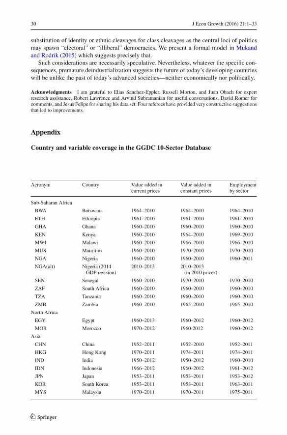
30 J Econ Growth (2016) 21:1–33

substitution of identity or ethnic cleavages for class cleavages as the central loci of politicsmay spawn “electoral” or “illiberal” democracies. We present a formal model in Mukandand Rodrik (2015) which suggests precisely that.

Such considerations are necessarily speculative. Nevertheless, whatever the specific con-sequences, premature deindustrialization suggests the future of today’s developing countrieswill be unlike the past of today’s advanced societies—neither economically nor politically.

Acknowledgments I am grateful to Elias Sanchez-Eppler, Russell Morton, and Juan Obach for expertresearch assistance, Robert Lawrence and Arvind Subramanian for useful conversations, David Romer forcomments, and Jesus Felipe for sharing his data set. Four referees have provided very constructive suggestionsthat led to improvements.

Appendix

Country and variable coverage in the GGDC 10-Sector Database

Acronym Country Value added incurrent prices

Value added inconstant prices

Employmentby sector

Sub-Saharan Africa

BWA Botswana 1964–2010 1964–2010 1964–2010

ETH Ethiopia 1961–2010 1961–2010 1961–2010

GHA Ghana 1960–2010 1960–2010 1960–2010

KEN Kenya 1960–2010 1964–2010 1969–2010

MWI Malawi 1960–2010 1966–2010 1966–2010

MUS Mauritius 1960–2010 1970–2010 1970–2010

NGA Nigeria 1960–2010 1960–2010 1960–2011

NGA(alt) Nigeria (2014GDP revision)

2010–2013 2010–2013(in 2010 prices)

SEN Senegal 1960–2010 1970–2010 1970–2010

ZAF South Africa 1960–2010 1960–2010 1960–2010

TZA Tanzania 1960–2010 1960–2010 1960–2010

ZMB Zambia 1960–2010 1965–2010 1965–2010

North Africa

EGY Egypt 1960–2013 1960–2012 1960–2012

MOR Morocco 1970–2012 1960-2012 1960–2012

Asia

CHN China 1952–2011 1952–2010 1952–2011

HKG Hong Kong 1970–2011 1974–2011 1974–2011

IND India 1950–2012 1950–2012 1960–2010

IDN Indonesia 1966–2012 1960–2012 1961–2012

JPN Japan 1953–2011 1953–2011 1953–2012

KOR South Korea 1953–2011 1953–2011 1963–2011

MYS Malaysia 1970–2011 1970–2011 1975–2011

123

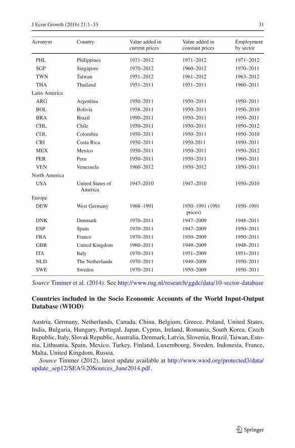
J Econ Growth (2016) 21:1–33 31

Acronym Country Value added incurrent prices

Value added inconstant prices

Employmentby sector

PHL Philippines 1971–2012 1971–2012 1971–2012

SGP Singapore 1970–2012 1960–2012 1970–2011

TWN Taiwan 1951–2012 1961–2012 1963–2012

THA Thailand 1951–2011 1951–2011 1960–2011

Latin America

ARG Argentina 1950–2011 1950–2011 1950–2011

BOL Bolivia 1958–2011 1950–2011 1950–2010

BRA Brazil 1990–2011 1950–2011 1950–2011

CHL Chile 1950–2011 1950–2011 1950–2012

COL Colombia 1950–2011 1950–2011 1950–2010

CRI Costa Rica 1950–2011 1950-2011 1950–2011

MEX Mexico 1950–2011 1950–2011 1950–2012

PER Peru 1950–2011 1950–2011 1960–2011

VEN Venezuela 1960–2012 1950–2012 1950–2011

North America

USA United States ofAmerica

1947–2010 1947–2010 1950–2010

Europe

DEW West Germany 1968–1991 1950–1991 (1991prices)

1950–1991

DNK Denmark 1970–2011 1947–2009 1948–2011

ESP Spain 1970–2011 1947–2009 1950–2011

FRA France 1970–2011 1950–2009 1950–2011

GBR United Kingdom 1960–2011 1949–2009 1948–2011

ITA Italy 1970–2011 1951–2009 1951–2011

NLD The Netherlands 1970–2011 1949–2009 1950–2011

SWE Sweden 1970–2011 1950–2009 1950–2011

Source Timmer et al. (2014). See http://www.rug.nl/research/ggdc/data/10-sector-database

Countries included in the Socio Economic Accounts of the World Input-OutputDatabase (WIOD)

Austria, Germany, Netherlands, Canada, China, Belgium, Greece, Poland, United States,India, Bulgaria, Hungary, Portugal, Japan, Cyprus, Ireland, Romania, South Korea, CzechRepublic, Italy, SlovakRepublic, Australia, Denmark, Latvia, Slovenia, Brazil, Taiwan, Esto-nia, Lithuania, Spain, Mexico, Turkey, Finland, Luxembourg, Sweden, Indonesia, France,Malta, United Kingdom, Russia.

Source Timmer (2012), latest update available at http://www.wiod.org/protected3/data/update_sep12/SEA%20Sources_June2014.pdf.

123

32 J Econ Growth (2016) 21:1–33

References

Acemoglu, D., & Robinson, J. (2009). Economic origins of dictatorship and democracy. Cambridge: Cam-bridge University Press.

African Center for Economic Transformation. (2014). Africa Transformation Report, 2014. Accra, Ghana.Amirapu, A., & Subramanian, A. (2015).Manufacturing or services? An indian illustration of a development

dilemma. Washington, DC: Center for Global Development and Peterson Institute.Baumol, W. J. (1967). Macroeconomics of unbalanced growth: The anatomy of urban crisis. The American

Economic Review, 57(3), 415–426.Baumol, W. J., & Bowen, W. G. (1965). On the performing arts: The anatomy of their economic problems.

The American Economic Review, 55(1/2), 495–502.Buera, F. J., & Kaboski, J. P. (2009). Can traditional theories of structural change fit the data? Journal of the

European Economic Association, 7(2—-3), 469–477.Corden, W. M. (1984). Booming sector and Dutch disease economics: Survey and consolidation. Oxford

Economic Papers, New Series, 36(3), 359–380.Dasgupta, S., & Singh, A. (2006). Manufacturing, services and premature deindustrialization in developing

countries: AKaldorian analysis. UNU-WIDER, United Nations University Research Paper, No. 2006/49.de Vries, K., Timmer,M. P., & deVries, G. J. (2013). Structural transformation in Africa: Static gains, dynamic

losses, GGDC research memorandum GD-136. Groningen Growth and Development Centre, Universityof Groningen.

Felipe, J., Mehta, A., & Rhee, C. (2014). Manufacturing matters... but it’s the jobs that count. Asian Develop-ment Bank Economics Working Paper Series, No. 420.

Foellmi, R., & Zweimuller, J. (2008). Structural change. Engel’s consumption cycles and Kaldor’s facts ofeconomic growth. Journal of Monetary Economics, 55, 1317–1328.

Franck, R., & Galor, O. (2015). Is industrialization conducive to long-run prosperity? Brown University,unpublished paper.

Kaldor, N. (1966). Causes of the slow rate of economic growth of the United Kingdom: An inaugural lecture.Cambridge (England): Cambridge University Press.

Lawrence, R. Z., & Edwards, L. (2013). US Employment deindustrialization: Insights from history and theinternational experience. Peterson Institute for International Economics, Policy Brief No. PB13-27.

Lind, J. T., &Mehlum, H. (2010). With or without u? Theappropriate test for a U-shaped relationship.Oxford-Bulletin of Economics and Statistics, 72(1), 109–118.

Maddison, A. (2009). Statistics on World Population, GDP and Per Capita GDP, 1-2008 AD. Available athttp://www.ggdc.net/maddison/oriindex.htm.

Matsuyama, K. (1992). Agricultural productivity, comparative advantage, and economic growth. Journal ofEconomic Theory, 58(2), 317–334.

Matsuyama, K. (2009). Structural change in an interdependent world: A global view of manufacturing decline.Journal of the European Economic Association, 7(2—-3), 478–486.

McMillan, M., & Rodrik, D. (2011). Globalization, structural change, and economic growth. InM. Bachetta &M. Jansen (Eds.), Making globalization socially sustainable. Geneva: International Labor Organizationand World Trade Organization.

McMillan, M., Rodrik, D., & Verduzco-Gallo, Í. (2014). Globalization, structural change, and productivitygrowth, with an update on Africa. World Development, 63, 11–32.

Mukand, S., & Rodrik D. (2015). The political economy of liberal democracy. Unpublished paper.Ngai, L. R., & Pissarides, C.A. (2004). Structural change in a multi-sector model of growth. Center for

Economic Performance, London School of Economics.Nickell, S., Redding, S., & Swaffield, J. (2008). The uneven pace of deindustrialization in the OECD. Center

for Economic Performance, London School of Economics.Palma, J. G. (2014). Industrialization, ‘premature’ deindustrialization and the Dutch disease. Revista NECAT,

3(5), 7–23.Rodríguez-Clare, A. (1996). The division of labor and economic development. Journal of Development Eco-

nomics, 49(1), 3–32.Rodrik, D. (1996). Coordination failures and government policy: A model with applications to East Asia and

Eastern Europe. Journal of International Economics, 40(1–2), 1–22.Rodrik, D. (2013). Unconditional convergence in manufacturing. Quarterly Journal of Economics, 128(1),

165–204.Rodrik, D. (2014). The past, present, and future of economic growth. In F. Allen, et al., Towards a better global

economy: Policy Implications for Citizens Worldwide in the 21st Century. Oxford: Oxford UniversityPress.

123

J Econ Growth (2016) 21:1–33 33

Sachs, J.D.,&Warner,A.M. (1999). Thebig push, natural resource booms andgrowth. Journal ofDevelopmentEconomics, 59(1), 43–76.

Timmer, Marcel P., de Vries, G.J., & de Vries, K. (2014). “Patterns ofStructural Change in DevelopingCountries,” Groningen Growth andDevelopment Center Research Memorandum 149.

Timmer,M. P. (Ed.). (2014). Theworld input-output database (WIOD): Contents, sources andmethods.WIODWorking Paper Number 10.

Uy, T., Yi, K.-M., & Zhang, J. (2013). Structural change in an open economy. Journal of Monetary Economics,60(6), 667–682.

van Wijnbergen, S. (1984). The ‘dutch disease’: A disease after all?’. The Economic Journal, 94(373), 41–55.Venables,A. J. (1996). Trade policy, cumulative causation, and industrial development. Journal ofDevelopment

Economics, 49(1), 179–197.Veugelers, R. (Ed.). (2013). Manufacturing Europe’s future. Brussels: Bruegel.World Trade Organization (2010).Measuring trade in services. Geneva: WTO.Young, A. Structural transformation, the mismeasurement of productivity growth, and the cost disease of

services. American Economic Review, forthcoming.Young, A. (2013). Inequality, the urban-rural gap, and migration.Quarterly Journal of Economics, 128, 1727–

1785.

123