preliminary results of the 2005 nata model-to …...preliminary results of the 2005 nata...
TRANSCRIPT

Preliminary Results of the 2005 NATA Model-to-Monitor Comparison
Regi Oommen, Stacie Enoch, and Robin Mongero Weyl
Eastern Research Group, Inc. (ERG), 1600 Perimeter Park Drive, Morrisville, NC 27560
Ted Palma, Barbara Driscoll, and Anne Pope
U.S. Environmental Protection Agency, USEPA Mailroom, Mail Code: C304-06, Research Triangle
Park, NC 27711
ABSTRACT
Acute and chronic exposure to specific hazardous air pollutants (HAPs) can lead to cancer and/or
noncancer effects. Since the passage of the 1990 Clean Air Act Amendments (CAAA), the U.S.
Environmental Protection Agency (EPA), state, local, and tribal agencies have spent considerable time
and resources establishing regulations primarily through maximum achievable control technology
(MACT) and mobile source standards, to reduce emissions for hazardous air pollutants (HAPs).
Identification of the most important individual emission sources and source categories significantly
contributing to potential health risks is challenging for many air quality managers. Large reductions in
HAP emissions may not necessarily translate into significant reductions in health risk because toxicity
varies by pollutant. For example, acetaldehyde mass emissions are more than double acrolein emissions
on a national basis, according to EPA’s 2005 National Emissions Inventory (NEI). However, according
to the Integrated Risk Information System (IRIS), acrolein is 450 times more toxic in terms of
respiratory noncancer risk than acetaldehyde. Thus, it is important to account for the toxicity as well as
the mass of the targeted emissions when designing reduction strategies to maximize health benefits.
One important tool for air quality managers is EPA’s National-Scale Air Toxics Assessment (NATA),
which uses HAP emissions from the NEI, meteorological data, background concentrations, population
densities, and pollutants specific health data to calculate census-tract level toxicity risk by HAP and
source category.
This paper analyzes the model performance of the 2005 NATA through a model-to-monitor
comparison, in which receptor-level concentrations calculated from the NATA model are compared to
2005 annual average concentrations of individual HAPs for several hundred air toxics monitoring sites
across the country. The preliminary results are summarized by HAP, and are important in understanding
the strengths and limitations of air toxics modeling.
INTRODUCTION
Acute and chronic exposure to specific hazardous air pollutants (HAPs) can lead to cancer and/or
noncancer effects. Since the passage of the 1990 Clean Air Act Amendments (CAAA),1 EPA has spent
considerable time and resources establishing federal regulations, primarily through maximum achievable
control technology (MACT) standards and Risk and Technology Review (RTR) activities, to reduce
emissions for HAPs. Atmospheric models, such as those executed for the National-Scale Air Toxics
Assessment (NATA), are often used to characterize the nation’s air toxics problem both in absolute as
well as relative senses by geographic area and pollutant.
The most robust method for assessing what people may be breathing is through ambient air
monitoring of HAPs. Ambient monitoring data can help identify pollutants and specific emission
sources impacting an area’s air quality, and track changes or identify trends in ambient concentrations.

Since 1990, the number of nationwide HAP monitors across the U.S. has increased dramatically (>50%).
As a consequence, an increase representativeness of people’s inhalation exposure to HAPs has
increased. However, the majority of HAP monitors are generally clustered in urban areas. For example,
2005 ambient air monitoring for benzene, a national priority pollutant, occurred mainly in urban areas
(Figure 1), accounting for less than 7% of all the counties in the country. This clustering of HAP
monitors highlights the geographic disparity in truly assessing nationwide exposure.
Due to the resources required for ambient monitoring of HAPs, it is not feasible to place
monitors all over the country, let alone in each county. However, EPA develops point source and
county-level source emission inventories for all geographic areas in the country. Thus, emissions
modeling can be performed to generate model ambient concentrations. NATA modeling is the “bridge”
to assess national-level exposure trends at all geographic locations across the country.
This paper demonstrates the approach for the model-to-monitor comparison, as well as
preliminarily evaluating the strengths/limitations of modeling specific HAPs. The following three
questions were used to guide the study:
1. Which pollutants are in good agreement between the ambient concentrations and the NATA
model?
2. Which pollutants are under-predicted between the ambient concentrations and the NATA
model?
3. Which pollutants are over-predicted between the ambient concentrations and the NATA
model?
DATA SOURCES
National-Scale Air Toxics Assessment (NATA)
NATA is EPA’s ongoing comprehensive evaluation of air toxics in the U.S. EPA developed the
NATA as a state-of-the-science screening tool for State/Local/Tribal Agencies to prioritize pollutants,
emission sources and locations of interest for further study in order to gain a better understanding of
risks.2 NATA assessments do not incorporate refined information about emission sources, but rather,
use general information about sources to develop estimates of risks which are more likely to
overestimate impacts than underestimate them. NATA provides estimates of the risk of cancer and other
serious health effects from breathing (inhaling) air toxics in order to inform both national and more
localized efforts to identify and prioritize air toxics, emission source types and locations which are of
greatest potential concern in terms of contributing to population risk. This in turn helps air pollution
experts focus limited analytical resources on areas and/or populations where the potential for health risks
are highest. Assessments include estimates of cancer and non-cancer health effects based on chronic
exposure from outdoor sources, including assessments of non-cancer health effects for Diesel Particulate
Matter (PM). Assessments provide a snapshot of the outdoor air quality and the risks to human health
that would result if air toxic emissions levels remained unchanged.
EPA made several methodological changes to its most recent assessment, the 2005 NATA.
Although EPA is continually refining and updating the assessment methods, it is important to remember
that NATA is a screening-level assessment. The intent is to identify HAPs resulting in high exposures
or census tracts where population exposures may be of concern. These areas would then require more
refined assessments, e.g., monitoring or site-specific risk assessments, to develop a more thorough
understanding of these “hot-spot” exposures.

NATA 2005 Improvements
The following improvements have been made in the 2005 NATA:3
1. Point Sources
a. The point source NATA inventory was based on 2005 emissions.
b. Risk and Technology Review emissions inventory updates were included.
c. Certain nonpoint categories are now modeled as point sources (i.e., forest and
wildfires, chromium electroplating).
d. Data for 19,000 airports were included.
2. Nonpoint sources
a. The 2005 NEI was generally unchanged from 2002 (few minor edits).
b. Emissions from forest fires, wildfires, and chromium electroplating were removed.
c. Formaldehyde and benzene from pesticides were removed from the 2005 NEI
inventory.
d. Chromium Electroplating sources were moved to the point source inventory.
e. Several minor adjustments to improve accuracy were made at the state/county level.
3. Mobile Sources
a. The onroad and nonroad inventories were updated for 2005.
b. The new MOVES (Motor Vehicle Emission Simulator) emissions model was used for
some HAPs.
4. Modeling
a. The secondary formation of formaldehyde, acetaldehyde, and acrolein were predicted
using Community Multi-Scale Air Quality (CMAQ) model.
b. The transformation of 1,3 butadiene to acrolein was accounted for using CMAQ.
c. The mobile source modeling approach using AERMOD was improved.
d. Emissions buoyancy for certain sources at coke oven facilities was accounted for.
5. Risk Characterization
a. Dose-response values were updated with latest science (IRIS, CalEPA, ATSDR).
b. The formaldehyde unit risk estimate was revised.
In addition to the census-tract level ambient concentrations predicted by the NATA 2005, EPA
used the model to develop specific receptor-level HAP concentrations for over 1,000 locations which
coincided with air toxics monitoring sites. These concentrations were the basis for the model-to-monitor
comparison.
National Emissions Inventory (NEI)
EPA compiles the NEI, consisting of stationary (point and nonpoint area), mobile (onroad and
nonroad), and biogenic source emissions for the entire United States.4 These emission inventories are
typically compiled for three years. Primary data sources for the point source NEI include:
1. State, local, and tribal agency emission inventories;
2. EPA’s SPPD and Risk and Technology Review (RTR) Programs;
3. Department of Energy’s (DOE) Energy Information Agency (EIA) and EPA’s Clean Air
Markets Division (CAMD) Emission Tracking System/Continuous Emissions Monitoring
(ETS/CEM) data for electric generating utilities (EGUs);
4. EPA’s Toxic Release Inventory (TRI); and
5. Data from other studies (e.g., trade associations, Bureau of Ocean Energy Management,
Regulation, and Enforcement (BOEMRE) oil and natural gas platform data).

Pollutants in the NEI consist of HAPs and criteria air pollutants (CAPs) and their precursors
(CO, NH3, NOx, PM, SO2, and VOCs). Base year inventories are typically compiled every three years;
the first NATA was for the 1996 NEI, with subsequent assessments in 1999 and 2002. EPA recently
finished preparing the 2005 HAP emissions for the 2005 NATA.5
Ambient Monitoring Data
Air toxics ambient monitoring data were extracted from EPA’s Phase VI Air Toxics Archive.
6
This archive contains over 26 million HAP concentration records, spanning from 1973 to 2007. For
2005, there were over 2.9 million HAP ambient records at varying measurement levels (1-hour, 3-hour,
4-hour, and 24-hour measurements) at over 800 monitoring sites. Nearly 92% of the HAP records for
2005 sampling dates were originally retrieved from EPA’s Air Quality Subsystem (AQS) and less than
7% were extracted from the Interagency Monitoring of Protected Visual Environments (IMPROVE).
The remaining data records (less than 2%) were taken from EPA’s Phase V historical archive.7
METHODOLOGY
Calculating Annual Averages
To properly compare ambient monitoring data to the modeled receptor concentrations, annual
average concentrations which represent the year 2005 must be calculated. Because the emissions that
were modeled were annual estimates, the model-to-monitor comparison must also reflect concentrations
for an entire year. Thus, from a temporal standpoint, it is not suitable to compare modeled
concentrations (which are modeled from annual emissions) to ambient data that do not represent an
entire year.
Annual averages are calculated using the following procedure:
1. Extract 2005 ambient HAP data from the Phase VI archive.
2. For sub-daily measurements, calculate valid daily concentrations.
3. Identify daily concentrations by site and pollutant which represent an entire year.
4. For non-detects, a zero was used as a surrogate.
5. Calculate annual average by HAP by site from the daily averages (including zeroes for non-
detects).
Calculating Daily Averages
Over 2.9 million concentration records were extracted for the 2005 year from the Phase VI
archive. Because these records were at differing temporal measurements, all records were converted to
daily records. Sub-daily measurements (over 55% of the 2005 records) must have at least 75% temporal
coverage within a day. Thus, to be considered a valid daily average:
1. At least eighteen of twenty-four 1-hour measurements must have a detected concentration.
2. At least six of eight 3-hour measurements must have a detected concentration.
3. At least five of six 4-hour measurements must have a detected concentration.
Calculating Annual Averages
Valid daily averages were then reviewed by site and HAP to assess whether there was adequate
temporal coverage. To assess temporal coverage, we used a two-step procedure.
1. Ensured that within each calendar quarter (January 1-March 31, April 1-June 30, July 1-
September 30, and October 1-December 31), six of eight prescribed sub-quarter zones by site
and HAP must have a valid daily concentration.
a. This approach allowed monitoring data which sampled once every twelve days
(which, in theory, yields a minimum of seven sampling days in a calendar quarter).
b. Sites which sampled more frequently than once every twelve days, such as 1-in-6
days or 1-in-3 days, will have more opportunity to meet this “sub-quarter zone”
temporal coverage.
2. Ensured that a valid annual average by site and HAP consisted of three valid calendar
quarters.
An annual average is simply the average of detected concentrations and non-detects which
satisfied the above procedure. For non-detects, a zero value was used as a surrogate prior to calculating
valid annual averages. This is another deviation from the 2002 NATA model-to-monitor comparison
which used one-half the pollutant method detection limit as a surrogate for non-detects in calculating the
annual average.8
PRELIMINARY RESULTS
Table 1 presents the number of monitoring sites used in the 2005 comparison, the 25th, 50
th, and
75th
ratios of the model-to-monitor average concentrations, and the model-to-monitor average
concentration by HAP. The number of sites is the number of monitors with valid annual averages for
2005. A median ratio close to 1 implies the model overestimates the ambient concentrations about as
often as it underestimates them. Not surprisingly, HAPs with a large number of monitors tended to have
median model-to-monitor ratios closer to 1.
Only HAPs with a minimum of 25 monitors were included in this table. This is another
deviation from the 2002 model-to-monitor assessment which required a minimum of 50 monitors.8 In
the 2002 assessment, model-to-monitor ratios for the metals were presented for the PM2.5 and TSP size
fractions. For the 2005 assessment, it was decided that modeled metal concentrations would be better
compared to the PM10 size fraction. This is primarily because the vast majority of the PM2.5 ratios used
in the 2002 assessment were from monitors in the IMPROVE network, which were typically situated in
Federal Class 1 and Class 2 areas (e.g., national parks, protected areas) where typical emission sources
are not found, and where people do not live. In 2005, PM10 metals measurements were only being taken
at around 70 monitoring sites, as opposed to over 400 PM2.5 metals monitoring sites; thus, the minimum
number of monitoring sites required needed to be reduced in order to characterize modeled metal
concentrations. Finally, the number of monitoring sites measuring for PM10 metals has been increasing
since 2005, especially in urban areas, and will continue to serve as a better comparison for modeled
metal concentrations in future assessments.
Carbon tetrachloride, methyl chloride, and arsenic (PM10) all had median ratios between 0.9 to
1.1. The percent of sites estimated “within a factor of 2” is the percent of sites for which the model
estimate is somewhere between half and double the monitor average. HAPs in which 80% of their
monitors were within a factor of 2 were benzene (82%), carbon tetrachloride (95%), methyl chloride
(92%), and acetaldehyde (87%).
The “percent of sites estimated within 30%” is the percent of sites for which the model-to-
monitor media ratio is between 0.7 and 1.3. Finally, the “percent of sites underestimated” is the percent
of sites for which the model-to-monitor ratio is below 1.

Figures 1 through 3 present the distribution statistics (25th
, 50th, 75
th, and average model-to-
monitor ratios) for each HAP. Figure 1 presents gaseous HAPs with greater than 100 monitors, while
Figure 2 presents gaseous HAPs with less than 100 monitors. Finally, Figure 3 presents metal HAPs.
For example, if there are 295 monitors with valid annual average concentrations of benzene, there are
295 model-to-monitor ratios to compute. EPA then computed the median of these 295 ratios as well as
the percentiles to create the plot. The bottom of the statistic is the 25th percentile, the top of the statistic
is the 75th percentile, the horizontal line in the middle is the median (i.e., 50
th percentile), and the “x” is
the average model-to-monitor ratio. The yellow area represents the “factor of two” range. If the model
consistently agrees with the monitored data for the pollutant, the 25th and 50
th percentile lines will be
narrow and centered at 1. Pollutants are organized alphabetically; this side-by-side display of pollutants
facilitates comparison to indicate which pollutants are being overestimated and underestimated, and
which are estimated consistently. As in the 1996, 1999, and 2002 comparisons, the box plots do not
show extreme percentiles (e.g., 10th
and 90th) of the ratios because the extreme percentiles were far from
the center of the distribution.
Approximately 9% of all model-to-monitor ratios were within 10 % (i.e., ratios between 0.9 and
1.1), 17% were within 20% (ratios between 0.8 and 1.2), and 25% were within 30% (ratios between 0.7
and 1.3). “Factor of 2” ratios (ratios between 0.5 and 2.0) accounted for 44% of the model-to-monitor
ratios.
These results show that the interquartile range of model-to-monitor comparisons was within a
factor of two for acetaldehyde, arsenic (PM10), benzene, carbon tetrachloride, formaldehyde, methyl
chloride, and toluene. The remaining pollutants show various degrees of agreement. These results are
similar to those found in the 2002 national-scale assessment comparisons. However, the model is still
underestimating several pollutants (i.e., 75th percentile ratio is below 0.5), most noticeably, ethylene
dichloride, n-hexane, 1,1,2-trichloroethane, acrylonitrile, carbon disulfide, chloroprene, 1,3-
dichloropropene, ethylene dibromide, ethylidene dichloride, methyl isobutyl ketone, propionaldehyde,
propylene dichloride, and vinylidene chloride.
As a whole, the PM10 metals appear to have good agreement with the NATA model, with the
exception of beryllium (PM10). Beryllium (PM10) was the only HAP to have its 25th
percentile ratio
above 2.
Data Considerations - Uncertainties
Earlier in this analysis, we identified several data and model improvements for the 2005 NATA.
These improvements are reflected in the increase of more pollutants approaching the median model-to-
monitor ratio closer to 1. However, there are areas in which the confidence of the model performance
can be improved. This confidence, or degree of agreement between model-to-monitor data, can be
attributed to the following five uncertainties (which are the same identified in the 1996, 1999, and 2002
model-to-monitor comparison):
1. Emission characterization uncertainties (e.g., specification of source location, emission rates,
and release characterization);
2. Meteorological characterization uncertainties (e.g., representativeness);
3. Model formulation and methodology uncertainties (e.g., characterization of dispersion,
plume rise, deposition,);
4. Monitoring uncertainties; and
5. Uncertainties in background concentrations.
Data Considerations – Under-estimation
Approximately 10% of all model-to-monitor ratios were between 0.9 and 1.1, while the number
of pollutants showed an increasing trend towards a median model-to-monitor ratio of 1, there were
several pollutants identified that were under-estimated. The 1996, 1999, and 2002 model-to-monitor
comparisons identified four possible reasons for pollutants to be under-estimated, which may be
applicable for the 2005 model-to-monitor assessment. They are:
1. The NEI may be missing specific emissions sources (emissions parameters are missing for
many of the sources in the NEI);
2. The emission rates may be underestimated. EPA believes the model itself contributed only in
a minor way to the underestimation. In many tests evaluating the model performance, the
modeled results compared favorably to monitoring data in cases where the emissions and
meteorology were accurately characterized and the monitors made more frequent readings;
3. There is uncertainty in the accuracy of the monitor averages, which, in turn, have their own
sources of uncertainty. Sampling and analytical uncertainty, measurement bias, and temporal
variation can all cause the ambient concentrations to be inaccurate or imprecise
representations of the true atmospheric averages; and
4. Background concentrations (pollutants transported large distances and/or formed by
photochemical processes in the atmosphere) are poorly characterized. Most of the pollutants
for which the model underestimated ambient concentrations were those for which
background concentrations were not estimated. If background concentrations are a large
fraction of ambient concentrations, the result would be large underestimations in model
predictions.
CONCLUSIONS
EPA recently completed its fourth national-scale assessment for air toxics across the United
States. In this paper, we evaluated model performance for several pollutants by comparing modeled
concentrations to monitored concentrations. Approximately 9% of all model-to-monitor ratios were
within 10 % (i.e., ratios between 0.9 and 1.1), 17% were within 20% (ratios between 0.8 and 1.2), and
25% were within 30% (ratios between 0.7 and 1.3).
The following three questions were used to guide the study:
� Which pollutants are in good agreement between the ambient concentrations and the NATA 2005 model? Good agreement (i.e., interquartile values within a factor of two) were seen for the
following pollutants: acetaldehyde, arsenic (PM10), benzene, carbon tetrachloride, formaldehyde,
methyl chloride, and toluene.
� Which pollutants are under-predicted between the ambient concentrations and the NATA 2005 model? Under-prediction (upper bound of the interquartile range less than a factor of two)
was seen for the following pollutants: ethylene dichloride, n-hexane, 1,1,2-trichloroethane,
acrylonitrile, carbon disulfide, chloroprene, 1,3-dichloropropene, ethylene dibromide, ethylene
dichloride, methyl isobutyl ketone, propionaldehyde, propylene dichloride, and vinylidene
chloride.
� Which pollutants are over-predicted between the ambient concentrations and the NATA 2005 model? Over-prediction (lower bound of the interquartile greater than a factor of two) was seen
for beryllium (PM10).

HAPs in which 80% of their monitors were within a factor of 2 were benzene (82%), carbon
tetrachloride (95%), methyl chloride (92%), and acetaldehyde (87%). “Factor of 2” ratios (ratios
between 0.5 and 2.0) accounted for 44% of the model-to-monitor ratios.
REFERENCES
1. U.S. EPA. Clean Air Act Amendments. OAQPS. Internet address:
http://www.epa.gov/air/oaq_caa.html/
2. U.S. EPA. National Air Toxics Assessment. OAQPS. Internet address: http://www.epa.gov/nata/
3. Palma, T. E-mail Communication from Ted Palma, U.S. EPA to Regi Oommen, Eastern Research
Group. September 7, 2010.
4. U.S. EPA. Emissions Inventories. OAQPS. Internet address:
http://www.epa.gov/ttn/chief/eiinformation.html
5. U.S. EPA. 2005 NATA National Emissions Inventory (NEI), Version 3. Data provided by A. Pope.
OAQPS. August 2010.
6. U.S. EPA. Air Toxics Data. OAQPS. Internet address:
http://www.epa.gov/ttn/amtic/toxdat.html#data
7. U.S. EPA. Air Toxics Data Analysis 2003-2006 (partial). OAQPS. Internet address:
http://www.epa.gov/ttn/amtic/toxdat.html#data
8. U.S. EPA. Comparison of the 2002 Model-Predicted Concentrations to Monitored Data. OAQPS.
Internet address: http://www.epa.gov/ttn/atw/nata2002/02pdfs/2002compare.pdf
KEYWORDS
Hazardous Air Pollutants (HAPs)
National Emissions Inventory (NEI)
Annual Averaging
Model Evaluation
Model-to-Monitor
National-Scale Air Toxics Assessment (NATA)

Figure 1. Benzene Emission Sources and Monitoring Sites in 2005.
(
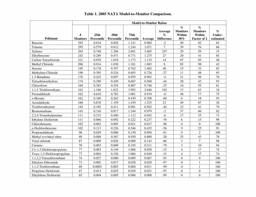
Table 1. 2005 NATA Model-to-Monitor Comparison.
Model-to-Monitor Ratios
Pollutant #
Monitors
25th
Percentile
50th
Percentile
75th
Percentile Average
Average
%
Difference
%
Monitors
Within
30%
%
Monitors
Within
Factor of 2
%
Under-
estimated
Benzene 295 0.634 0.826 1.141 0.984 -2 49 82 65
Toluene 295 0.579 0.812 1.244 1.071 7 39 76 66
Xylenes 265 0.748 1.284 2.041 3.465 247 29 59 33
Ethylbenzene 242 0.289 0.471 0.771 1.275 27 20 41 85
Carbon Tetrachloride 221 0.939 1.018 1.173 1.135 14 87 95 48
Methyl Chloride 206 0.914 1.030 1.181 1.083 8 85 98 42
Styrene 195 0.178 0.397 0.762 1.402 40 15 32 83
Methylene Chloride 190 0.395 0.524 0.693 0.726 -27 11 48 85
1,3-Butadiene 176 0.425 0.697 0.955 0.962 -4 31 56 76
Tetrachloroethylene 174 0.289 0.449 0.687 0.560 -44 20 42 93
Chloroform 169 0.383 0.554 0.807 0.746 -25 18 55 81
1,1,1-Trichloroethane 163 1.166 1.622 3.993 2.646 165 13 63 18
Formaldehyde 162 0.610 0.783 1.001 0.919 -8 48 77 75
n-Hexane 162 0.160 0.262 0.439 0.398 -60 6 18 93
Acetaldehyde 160 0.878 1.159 1.439 1.235 23 49 87 36
Trichloroethylene 145 0.185 0.411 0.901 0.562 -44 22 41 79
Bromomethane 143 0.316 0.817 1.244 0.979 -2 37 66 62
2,2,4-Trimethylpentane 111 0.215 0.490 1.112 0.942 -6 17 35 73
Ethylene Dichloride 111 0.066 0.092 0.222 0.237 -76 6 15 98
Chlorobenzene 102 0.003 0.005 0.021 0.017 -98 0 0 100
p-Dichlorobenzene 102 0.113 0.226 0.546 0.435 -56 9 25 91
Propionaldehyde 98 0.029 0.060 0.130 0.094 -91 0 2 100
Methyl tert-butyl ether 88 0.088 0.567 0.930 0.800 -20 25 43 78
Vinyl chloride 87 0.009 0.026 0.089 0.143 -86 3 7 98
Cumene 78 0.003 0.009 0.195 0.211 -79 3 10 94
Cis-1,3-Dichloropropylene 77 0.003 0.149 1.066 0.850 -15 4 17 74
Trans-1,3-Dichloropropylene 77 0.004 0.156 1.066 0.849 -15 4 17 74
1,1,2,2-Tetrachloroethane 74 0.027 0.080 0.089 0.067 -93 0 0 100
Ethylene Dibromide 73 0.005 0.017 0.028 0.029 -97 0 1 100
1,1,2-Trichloroethane 69 0.0003 0.003 0.004 0.011 -99 0 1 100
Propylene Dichloride 67 0.013 0.025 0.038 0.031 -97 0 0 100
Ethylidene Dichloride 65 0.004 0.005 0.006 0.008 -99 0 0 100

Table 1. 2005 NATA Model-to-Monitor Comparison (Cont.).
Model-to-Monitor Ratios
Pollutant #
Monitors
25th
Percentile
50th
Percentile
75th
Percentile Average
Average
%
Difference
%
Monitors
Within
30%
%
Monitors
Within
Factor of 2
%
Under-
estimated
Vinylidene Chloride 65 0.001 0.004 0.004 0.011 -99 0 0 100
Methyl Isobutyl Ketone 63 0.019 0.105 0.486 5.386 439 2 11 86
Carbon disulfide 53 0.0002 0.002 0.007 0.010 -99 0 0 100
Acrolein 51 0.062 0.103 0.271 0.265 -74 4 10 96
Acrylonitrile 49 0.008 0.015 0.037 0.023 -98 0 0 100
Chloroprene 46 0.0003 0.004 0.005 0.003 -100 0 0 100
Manganese (PM10) 38 0.276 0.459 0.700 0.801 -20 13 37 84
Arsenic (PM10) 37 0.721 1.037 1.368 1.112 11 43 78 38
Lead (PM10) 37 0.448 0.623 0.870 0.704 -30 30 65 81
Nickel (PM10) 37 0.307 0.724 1.242 0.982 -2 32 46 57
Chromium (PM10) 36 0.265 0.455 0.879 0.984 -2 14 28 81
Cadmium (PM10) 32 0.683 1.179 1.859 1.320 32 31 69 41
Beryllium (PM10) 26 9.160 19.718 43.517 29.551 2855 8 8 8
Selenium (PM10) 26 0.196 0.381 0.597 0.518 -48 8 23 92
Cobalt (PM10) 25 0.346 0.490 1.612 1.117 12 16 32 64

Figure 2. Model-to-Monitor Comparisons of Gaseous HAPs (>100 Monitors)

Figure 3. Model-to-Monitor Comparisons of Gaseous HAPs (<100 Monitors)

Figure 4. Model-to-Monitor Comparisons of Metal HAPs