Preliminary and Incomplete

Cross Country Differences in Productivity: The Role of Allocative Efficiency

By Eric Bartelsman, John Haltiwanger and Stefano Scarpetta1

Draft: December 28, 2006

Abstract

There is a growing body of evidence suggesting that healthy, market economies exhibit both static and dynamic allocative efficiency, whereby more productive businesses have a larger market share and reallocation of outputs and inputs within sectors shifts resources from less to more productive businesses (e.g. Baily, Hulten, and Campbell (1992), Bartelsman, Haltiwanger, and Scarpetta (2004), Foster, Haltiwanger, and Krizan (2006), Olley and Pakes (1996)). Because there are no welfare or productivity gains to be obtained from resource reallocation in a frictionless economy (e.g. Hulten (1978); Levinsohn and Petrin (2006)), theoretical and empirical research is needed to model and quantify the frictions that yield a connection between reallocation and productivity. In this paper, we consider models that feature taste and technology differences so that a market with free entry sustains firms operating within a wide range of productivity (e.g, Restuccia and Rogerson (2004), and Hsieh and Klenow (2006)). We then investigate to what extent distortions in signals to decision makers generate model outcomes that track patterns of resource allocation and productivity observed across countries, sectors and over time.

1. Respectively: Vrije Universiteit Amsterdam and Tinbergen Institute; University of Maryland,

IZA, and NBER; the OECD and IZA, Bonn. We thank conference participants at NBER Summer Institute, July 2006, CAED Chicago, Sept. 2006, and DIME, London, Dec. 2006 for their useful comments and suggestions and Amil Petrin for detailed written comments. We are grateful to Karin Bouwmeester, Helena Schweiger, and Victor Sulla for excellent research assistance. The views expressed in this paper are those of the authors and should not be held to represent those of the OECD, the World Bank or its countries.

Introduction

There is a growing body of evidence suggesting that healthy, market economies exhibit both static and dynamic allocative efficiency, whereby more productive businesses have a larger market share and reallocation of outputs and inputs within sectors shifts resources from the less to more productive businesses (e.g., Baily, Hulten, and Campbell (1992), Bartelsman, Haltiwanger, and Scarpetta (2004), Foster, Haltiwanger, and Krizan (2006), Olley and Pakes (1996)). In an accounting sense, the contribution of reallocation to overall productivity is sizeable. Underlying this contribution of reallocation is the observation that there are large differences in productivity performance across firms even in narrowly defined industries. Empirical evidence suggests, for example, that the difference in total factor productivity between the 90th and the 10th percentiles within narrowly defined industries is about 65 log points in the United States, and for labor productivity is about 140 log points (see, e.g., Syverson (2004a). This wide dispersion in productivity provides considerable scope for reallocation in boosting aggregate productivity and growth.

The evidence of large dispersion in firm productivity and, in turn, of a sizeable contribution of allocative efficiency in market economies raises a variety of questions. The coexistence in narrowly-defined industries of firms with very different productivity performance is consistent with the idea of substantial frictions preventing resources from being immediately allocated to the highest valued use. Such frictions might arise from many factors. They may represent adjustment costs– either in the form of entry and exit costs, or costs in reallocating factors of production such as capital and labor (see, e.g., Hopenhayn (1992) and Hammermesh and Pfann (1996)). The latter include the search and matching frictions that have been the focus of much of the recent literature on studying the dynamics of the labor market (see e.g. Davis, Haltiwanger, and Schuh (1996), Mortensen and Pissarides (1994)). There may be static frictions that imply persistent productivity differences across producers in seemingly narrowly defined sectors. Product differentiation within sectors due to local markets is one such factor. For example, Syverson (2004a) explored the role of local markets for the U.S. concrete industry and found that variation in the market density across local markets significantly accounts for variation in the dispersion of productivity and prices across these markets.

Static and dynamic frictions partly depend on market characteristics and technological factors. However, frictions can also be driven by policy and institutions that affect market competition and adjustment costs (see e.g. World Bank, Doing Business, 2006)). While these issues are hardly resolved for advanced economies, they assume an even larger role in emerging and transition economies. These countries tend to have institutional factors that create greater distortions to the allocative process. These include implicit or explicit subsidies to favored incumbents or excessive and arbitrarily enforced regulations that make the cost of doing business inefficiently high (e.g., start up costs or opacity of business regulations). The infrastructure for doing business (e.g., communications and transportation infrastructure) may also weaken the efficiency of the allocation process. Moreover, graft and corruption that yields uneven application of rules and regulations are also likely to hinder allocative efficiency. All of these factors worsen

different aspects of the investment climate and affect the performance of private firms. In this paper, we emphasize the effects of dispersion in business climate conditions across producers within each country, since we are especially interested in the role of allocative efficiency.

The basic working hypothesis is that frictions play an important role in the allocative efficiency and, through this channel, to productivity and output growth. While some of these frictions are inherent even in well-developed market economies, others are affected by policy and institutional settings and thus could be tackled by appropriate reforms. The evidence of large dispersion in allocative efficiency even across OECD countries provides support to this claim. This is not a new hypothesis, and others have explored its implications in a variety of theoretical and empirical contributions (see e.g.,Banerjee and Duflo (2004), Restuccia and Rogerson (2004), and Hsieh and Klenow (2006)). Our contribution is to quantify the magnitude of allocative efficiency in a sample of industrial, and emerging economies drawing from a harmonized, cross country database with key measures and moments from firm-level data. Using a simple decomposition of industry-level productivity (Olley and Pakes (1996)), we find evidence of considerable cross country variation in allocative efficiency across countries. For example, we find that, in the United States, shifting from the existing firm allocation of market shares to one where shares are allocated randomly would yield a 50 percent loss in labor productivity within the average industry. Moreover, we find significant changes in allocative efficiency over time in the Eastern European countries during their transition to a market economy: market oriented reforms in these countries have led to an improvement in allocative efficiency equal to about 30-50 log points increase in labor productivity.

However, these empirical decompositions are only suggestive and require a more theoretical underpinning. Accordingly, we develop a simple model that draws heavily on the work of Restuccia and Rogerson (2004) and Hsieh and Klenow (2006). We calibrate this model to match the moments from our harmonized data and in particular the moments from the Olley-Pakes (hereafter OP) labor productivity empirical decomposition. We deliberately focus on these empirical decompositions since they have been used widely in the literature. We show in the numerical analysis of our model that, consistent with our working hypothesis, an increase in the cross-firm dispersion of distortions yields a decline in allocative efficiency as measured by the OP decomposition. We push this finding further by quantifying the magnitude of distortions that are needed to account for the variation in the observed OP measures, both between and within countries.

By exploring the theoretical underpinnings of the empirical decompositions that

have appeared in the literature, we also discuss how distortions can affect different margins of the reallocation process. Consistent with the intuitive explanation of the Olley-Pakes decompositions, we find that distortions tend to reduce the OP cross term – that is to say the covariance of market share and productivity level of a given set of market participants. However, there are additional margins impacted by distortions that are, potentially, even more important. For one, distortions may impact not only the

covariance for a given set of firms but also the selection process of market participants. The impact that market distortions can have on selection is nontrivial and has a variety of related implications. In a model where potential market participants must pay an entry fee before learning their productivity, distortions will affect the number of new firms that pay entry fees. Distortions can also affect the mix of firms and the scale of activity: for example, the average firm size and the capital-labor ratio. In addition, distortions impact the average unweighted productivity of those that do survive. All of these effects can have adverse impacts on consumption (or more generally welfare). The implication of these findings is that while measured allocative efficiency in terms of the OP cross term is a useful indicator it is by far not the only one for quantifying the impact of distortions on market economies.

The paper proceeds as follows. Section 2 describes the harmonized firm level database. Section 3 presents some basic facts about productivity dispersion within the countries in our database as well as the patterns of allocative efficiency as measured by the OP decomposition. Section 4 develops the model of allocative efficiency with distortions in the allocative process. Section 5 calibrates the model numerically to explore its implications in light of the empirical patterns in section 3. Section 6 presents concluding remarks.

2. The harmonized firm-level database and indicators of dispersion To assess the degree of firm heterogeneity, the magnitude and characteristics of resource reallocation and, ultimately, their impact on sectoral and aggregate productivity, we use a harmonized firm-level database that covers 24 industrial and emerging economies.2 These data have been collected from micro data from business registers, census and enterprise surveys playing particular attention at harmonizing, to the extent possible, key concepts (e.g. entry, exit, or the definition of the unit of measurement) as well as at using common methods to compute the indicators. A detailed technical description of the dataset may be found in Bartelsman, Haltiwanger, and Scarpetta (2005).3

The database contains information on firm demographics, such as entry and exit, jobs flows, size distribution and firm survival, as well as on productivity distributions and correlates of productivity. In particular, information was collected on the distribution of labor and/or total factor productivity by industry and year and on the decomposition of productivity growth into within-firm and reallocation components. Further, information is provided on the averages of firm-level variables by productivity quartile, industry, and

2 The dataset includes 10 OECD countries: (Canada, Denmark, Germany, Finland, France, Italy,

the Netherlands, Portugal, United Kingdom and United States) and 14 transition and emerging economies (Estonia, Hungary, Latvia, Romania, Slovenia; Argentina, Brazil, Chile, Colombia, Mexico, Venezuela, Indonesia, South Korea and Taiwan.(China)). However, different parts of the analysis use a smaller sub-set of countries due to data availability.

3 The analysis of firm demographics is based on business registers, census, social security databases, or employment-based register containing information on both establishments and firms. Data for the analysis of productivity growth come more frequently from business surveys.

year. The classification into about 40 sectors (roughly the 2-digit level detail of ISIC Rev3) coincides with the OECD Structural Analysis (STAN) database.4

For the purposes of this paper, we consider two indicators of dispersion that are particularly relevant. First, we look at the distribution of firm by size across industries and countries. The observed wide -- and largely skewed towards small units -- distribution of firm size shows ample room for allocative efficiency to play a role. An open empirical question in the presence of within-industry size dispersion is whether the large (small) firms are more (less) productive. An accompanying requirement for allocative efficiency effects to be important is to have productivity dispersion across firms. The database provides information on the distribution of firm productivity by industry, country and time, as well.

• Heterogeneity in firm size among incumbents: Table 1 presents the ratio of the average size of the top to the bottom quartile of the distribution of firms by size in the total economy and the manufacturing sector. The table suggests a wide dispersion in firm size in all countries for which data are available. Moreover, in most countries the dispersion is larger in the manufacturing sector than in the total business sector and, within manufacturing, in high-tech industries compared with the manufacturing average. It should be stressed, however, that the cross-country comparison of firm size dispersion may be influenced by the overall dimension of the internal market – especially for non-tradeables – and by the different sectoral composition of each country. The data indeed suggest wider dispersion in firm size in some of the large economies – e.g. the United States – but also in some of the transition economies in Eastern Europe, where policy-induced distortions have allowed the survival of very large (formerly or still) state-owned firms together with many new smaller private units. In Annex Table 1, we present indicators of firm size dispersion after controlling for industry composition. Within 2-3 digit manufacturing industries, the inter-quartile ratio of average firm size is still considerable in all industries and countries.

• Dispersion in labor productivity and MFP: There are also wide differences in firms’ productivity performance within manufacturing industries. Table 2 presents the difference between the top and bottom quartile of the log labor productivity within industries. The differences are in the range of 120-250 log points in most countries. Part of the significant cross-country differences is due to differences in the sectoral composition (see column 2 in the Table), but even controlling for that, the gap in labor productivity between the most and the least productive firms remains wide. And, as in the case of the dispersion in firm size, the high-tech sectors tend to be characterized by an even higher dispersion in all countries, suggesting that where there is more room for innovation and market experimentation there is more heterogeneity in firm characteristics and performance. To confirm this, Table 3 and Table 4 present the standard deviations in labor and multifactor productivity levels across firms for the different manufacturing industries. They clearly point to major differences in performances

4. See www.oecd.org/data/stan.htm

across all industries and countries. The data also suggest a wider dispersion in labor than in MFP for all the countries for which we have data (Figure 1).

3. Empirical Measures of Allocative efficiency

How does the observed heterogeneity in firm characteristics and performance affect aggregate productivity? To address this question, we look at measures of allocative efficiency within industries using an indicator originally proposed by Olley and Pakes (1996). They note that in a cross section of firms at a given point in time, the level of productivity for a sector can be decomposed as follows:

(1/ ) ( )( )t t it it t it ti i

P N P P Pθ θ= + − −∑ ∑

where Pt is sectoral productivity, Pit is firm-level productivity, itθ is the share of activity of the firm, Nt is the number of businesses in the sector and a ‘bar’ over a variable represents the unweighted industry average of the firm-level measure. The simple interpretation of this decomposition is that aggregate productivity can be decomposed into two terms involving the un-weighted average of firm-level productivity plus a cross term that reflects the cross-sectional efficiency of the allocation of activity. The cross term captures allocative efficiency since it reflects the extent to which firms with higher than average productivity have a greater market share. Olley and Pakes used this decomposition to show that, following the deregulation of the telecommunications markets in the U.S. in the early 1980s, this cross term increased substantially in the industry when applying this methodology to plant-level measures of total factor productivity.

This decomposition is easy to implement as it involves measures of the un-weighted average productivity and of the weighted average productivity. Measurement problems make comparisons of the levels of either of these measures across sectors or countries potentially problematic, but taking the difference between these two measures reflects a form of a difference-in-difference approach. As such, in principle the OP cross term is comparable across countries since any measurement problem that affects productivity levels is differenced out by the indicator.

In most of the analysis in this paper, we use log labor productivity at the micro level as our measure of Pit, and the firm’s labor share in the industry as our measure of θit. 5 We focus on labor productivity because it is more readily available (and likely more 5 In implementing this decomposition we use log productivity at the micro level so that the aggregate

productivity at the industry level is a geometric mean. Use of a log based decomposition facilitates comparisons of this decomposition using weighted averages of the industry level decomposition over time and industry. That is, the OP cross term using logs is unit-free and other related differences are unit free. In a related way, the micro and aggregate measures compared at two points in time yield productivity growth measures with desirable properties (e.g., symmetric growth for positive and negative changes). The use of log productivity differs from the original Olley-Pakes (1996)

accurately measured) in our sample of countries. A number of studies (e.g., Eslava, Haltiwanger, Kugler, and Kugler (2004), and Foster, Haltiwanger, and Krizan (2001)) have shown that the patterns of the OP decomposition within a country are similar for labor productivity and total factor productivity when using the same market shares. In the numerically simulated model discussed in the next sections, we also use labor productivity to derive inferences on the impact of distortions on the patterns of allocative efficiency. The distribution of labor productivity as well as implied allocative efficiency measured in this way in the model will be endogenous and a function of distortions. In the calibration, we also consider the OP decomposition using TFP in the simulated data and other implications of the model including the impact on variables like log(consumption).

Figure 2 shows the results of applying the OP decomposition at the industry level and then taking the weighted average results by industry for the countries in the harmonized database. We focus our attention on the cross term -- or as we define it – the “allocative efficiency” term. We find that for virtually all countries the OP cross term is positive, suggesting a positive covariation between market share and productivity at the micro level within the average industry. For example, we find that allocative efficiency is slightly less than 0.50 in the U.S. within the average industry. Since productivity is measured in logs, this implies that, within the average U.S. manufacturing industry, labor productivity would be about 50 logs point smaller if labor were allocated randomly. The international comparison also suggests that the OP cross term is substantially higher in the U.S. than in most European countries. By contrast, there is evidence of high – if not higher – allocative efficiency in some East Asian economies. Latin American economies have lower cross terms than the U.S., but higher than most European economies and the transition economies have the lowest cross terms.

While the OP cross term avoids some of the standard problems of cross country comparisons of productivity, it is not immune from measurement problems that are country-specific. In particular, measurement error in the second moment of the productivity distribution within a given industry that systematically varies by country (e.g. because the firm level data are systematically noisier in one country than another) will impact the OP cross term. For example, classical measurement error can reduce the OP cross term since it will mimic a more random allocation of market shares with respect to productivity. This consideration suggests some caution in assessing the observed cross-country patterns of allocative efficiency presented in Figure 2. To tackle this issue, we also present the evolution of the OP cross term over time within a country. To the extent measurement error within a country is relatively stable over time, the within country variation over time in the OP cross term will difference out the country-specific second moment measurement error.

The transition economies offer a rich context for assessing the potential links between distortions and allocative efficiency. Over the period observed by the available

specification that used the level of productivity. Given their focus on a single industry in the U.S., concerns about units were not relevant.

.

data (the 1990s), these countries undertook systemic reforms in their transitions from central-planning to a market economy. Arguably, many distortions affected the different margins of resource allocation during central planning: from barriers to entry, to distorted allocation of resources across firms, sectors and geographical areas. These distortions were gradually reduced if not eliminated in the transition to a market economy. Figure 3 shows the within country variation over time for the transition economies of the OP cross term. Interestingly, except for Estonia which starts with a relatively high cross term, the OP cross term increases in the transition economies and, in many cases, substantially. For example, in both Hungary and Slovenia, the OP cross term increases by about 20 log points during the transition.

Another advantage of examining the OP cross term over time within countries is that the variation in the estimated allocative efficiency can be put in the context of the overall patterns of productivity growth. In other words, changes in allocative efficiency may take place in the context of increasing or decreasing labor productivity. Figure 4 shows the evolutions over time in the overall (aggregated from industry-level data) labor productivity, the un-weighted average labor productivity and the OP cross term for Hungary and Slovenia. Put in this context, the OP cross term has increased substantially but the overall and un-weighted productivity term have increased as well, and at a even faster pace in the case of Slovenia. Thus, it would be misleading to draw inferences from Figures 2 and 3 that the OP cross term accounts for most of the cross sectional or time series variation in productivity between and within countries.

The main points from Figures 2-4 are that the OP cross term is large, it varies substantially across countries (with associated concerns about measurement error) and within transition economies, at least, it has also increased substantially over time. In comparing these findings to the existing literature, as noted above, Olley and Pakes found a positive cross term using TFP as the measure of productivity in the U.S. telecommunications industry and that the cross term increased substantially following deregulation in the U.S. telecommunications industry. Eslava, Haltiwanger, Kugler, and Kugler (2004) found (also using TFP) that the OP cross term rose substantially within 3-digit Colombian industries in the 1990s – a period of substantial market reforms in Colombia. These findings in the literature along with Figures 2-4 suggest that the OP cross term is capturing allocative efficiency. However, since it is a simple empirical decomposition, this evidence is only suggestive. To help put structure on the results in Figures 2-4, we turn to a model of allocative efficiency and distortions in the next section.

4. A Simple Model of Allocative Efficiency

To guide our analysis of distortions and allocative efficiency we develop a simple model drawing heavily from Restuccia and Rogerson (2004) and Hsieh and Klenow (2006). Key features of the model are diminishing returns and heterogeneous production units (as in Hopenhayn (1992) and Hopenhayn and Rogerson (1993)) that face

idiosyncratic distortions (Restuccia and Rogerson (2004)). Since our model borrows heavily from the models in the recent literature we only sketch the model here.6 Starting with the behaviour of firms, we assume that firms produce according a production function given by: (1) ( ) , 1it i it itY A n f kγ α α γ−= − < where itY is output for firm in period t, iA is the firm specific time invariant productivity for firm i, itk is the amount of capital input of firm i at time t, itn is the employment, and f is overhead labor. Decreasing returns is assumed due to some unobserved fixed factor in a manner similar to Lucas (1978) where it is useful to think about this factor as managerial ability.7 The decreasing returns insures (as in Lucas (1978)) that the most productive firm/manager does not take over the market. The overhead labor implies that the distribution of labor productivity is not degenerate even in an economy without distortions (i.e., while the marginal product of labor will be set equal to the wage rate, the average product of labor will vary with scale given overhead labor). Firms maximize profits, within an environment with distortions to capital expenditures and nominal output, in each period given by: (2) (1 )( ) (1 )it i i it it t it i t itA n f k w n r kγ α απ τ κ−= − − − − − where iτ is the firm specific and time invariant distortion to revenue for firm i, iκ is the firm specific distortion to capital allocation, tw is the wage paid to homogenous workers, and ttt Rr δ+= , is the user cost of capital which equals the interest rate plus the rate of depreciation. In considering these distortions, iτ can be interpreted broadly to include any distortion that impacts the scale of a business, while iκ represents any distortion that impacts the factor mix of a business. In what follows, we call these distortions a "scale distortion" and a "factor mix distortion" respectively.

6 The model presented here is closer to that of Restuccia and Rogerson (2004) than Hsieh and Klenow

(2006) although we borrow from both models. One difference from Restuccia and Rogerson (2004) is that instead of a fixed operating cost each period we specify overhead labor which plays a similar role in forcing low productivity firms to exit. However, the presence of overhead labor also yields dispersion in labor productivity even in the absence of distortions. Two other differences from Restuccia and Rogerson (2004) are drawn from Hsieh and Klenow (2006). We allow two different forms of distortions and interpret them as distortions per se and not as taxes/subsidies with tax revenue.

7 In order to get dispersion, we require some curvature in profits. Here we assume decreasing returns but a reasonable alternative is to assume some degree of market power in, e.g., a differentiated product environment. Hsieh and Klenow (2006) assume the latter. In future drafts we will add a differentiated product structure to explore the role of such a structure for our results.

To make the model and analysis tractable, we assume a simple ex ante and ex post timing of information and decisions in any given period. Ex ante, before a new firm enters, we assume that firms do not know their production and distortion draws but they know the distribution of these idiosyncratic variables. There is a fixed cost of entry, given by ec , that new firms must pay to enter and to learn their draws from the joint ex ante distribution of productivity and distortions, ).,,( κτAG Once a firm learns their draws of , , and i i iA τ κ , their values remain constant. Firms discount the future at rate (1/(1 ))Rβ = + and face an exogenous probability of exiting in each period given by .λ Given free entry and the assumptions about the arrival of information, new firms enter up to the point where the expected discounted value of profits is just equal to the entry fee. Moreover, given that the draws are time invariant in the steady state, the present discounted value for an incumbent firm i ex post is given simply by: (3) ( , , ) ( , , ) /(1 )i i i i i iW A Aτ κ π τ κ ρ= − where

(1 ) /(1 )Rρ λ= − + In turn, the free entry condition is given by: (4)

, ,

max(0, ( , , )) ( , , ) 0ee

A

W W A dG A cτ κ

τ κ τ κ= − =∫

New firms with a low productivity and/or a high scale (or factor mix) distortion draw will immediately exit upon learning their draws if they cannot cover their fixed operating costs. In what follows, we find that the fraction of firms that survive upon learning their productivity and distortion draws is an important factor for assessing the consequences of distortions. This is not surprising since distortions influence the pace of churning of firms and in this model this is captured by the pace of entry (the number of firms deciding to pay the entry fee) and exit (the number of firms that exit upon learning their draws).

The optimal capital/labor allocation will depend on input prices and the idiosyncratic capital distortion. An operating firm will have capital and employment in the steady state given by:

(5)

1/(1 )

*

( )(1 ) (1 )

(1 )

i

it

rAwk

r

γγ αγ αα τ κα

κ

−−⎡ ⎤−⎛ ⎞− +⎢ ⎥⎜ ⎟⎝ ⎠⎢ ⎥=

⎢ ⎥+⎢ ⎥⎣ ⎦

(6) * * ( )(1 )it itrn f k

wγ ακ

α−= + +

Output and profits for the operating firm are given by (1) and (2). Note that in the absence of distortions and overhead labor equations (1), (5) and (6) immediately yield that there is no dispersion in labor productivity. Overhead labor yields dispersion in labor productivity, even in the absence of distortions. But with distortions we get even greater dispersion in labor productivity. To close the model we must describe labor supply and the behaviour of households and workers. In this case, this is relatively straightforward as a fixed number of households are assumed to supply labor inelastically so that aggregate labor supply is equal to sN . Aggregate labor demand is given by:

*

, ,

( , , ) ( , , )dt t

A

N n A d Aτ κ

τ κ μ τ κ= ∫

where ),,( κτμ A is the ex post joint distribution for operating firms of productivity and distortions.8 In equilibrium the number of firms and wages must satisfy both the free entry condition and that labor demand equals aggregate labor supply.

st

dt

e NNW == ,0 Aggregate consumption plus resources spent on entry and depreciation will equal aggregate output in the steady state:9

ttett YKcEC =++ δ Where Kt is the aggregate of capital of ex-post operating firms. Underlying this model is the standard assumption that households maximize utility and given the assumption of inelastic labor supply this is assumed to be given by for the representative household:

∑∞

=0)(

tt

t CUβ

Subject to the budget constraint: 8 See the discussion and analysis in Restuccia and Rogerson (2004) about why the ex post joint

distribution will be time invariant in steady state equilibrium. 9 In steady state gross investment is only equal to replacement investment.

∑∑∞

=

∞

=+ ++=−−+

001 )())1((

ttttttt

ttttt KrNwpKKCp πδ

Where tp is the time zero price of period t consumption, tw and tr are the period t rental prices of labor and capital measured relative to period t output, and tπ is the total profit from the operations of all plants. A standard result emerges from the first order conditions of this problem given by:

1)/1( −=−= βδtt rR So the real interest rate and rental cost of capital is pinned down by the discount factor for utility and the capital depreciation rate.10

5. Calibration of Model We explore calibrations of the model by choosing some “reasonable” parameters for the model and explore its numerical properties. This analysis helps us to understand the interactions in the model and the role of distortions.11 For our initial numerical explorations, we select:

• γ = 0.9, • α =0.1, • λ = .10, this is consistent with evidence of firm exit rates in the United States and

other OECD countries (Bartelsman, Scarpetta, and Schivardi (2005)) • R=.03, and δ =.12, consistent with long run real interest rates in OECD countries

and typical depreciation rates from national accounts. • f=0.01 ,log(ce)=12.43, 12 • Mean(log(A)) = 10.57 • Std Dev (log(A)) = 0.35

The latter two moments are associated with the ex ante distribution G(A,τ,κ). These parameters are roughly consistent with the micro evidence for the U.S. For purposes of calibration and estimation, we consider a base case without distortions

10 See Restuccia and Rogerson (2004) for further discussion. 11 In future drafts we plan to push harder on the calibration to match the moments from the empirical

analysis in sections 2 and 3. However, it is our sense based upon the current analysis that we will need to enrich the model on some dimensions in order to be able to push the analysis in this direction. We discuss the nature of the enrichments we think are necessary below.

12 Interestingly, even with a very modest overhead labor there is substantial selection as well as ex post dispersion in labor productivity especially in environments with distortions. In future drafts, we plan to estimate these parameters using a simulated method of moments to match moments from the actual data.

(which might be thought of as the U.S.) and then ask whether we can account for the type of variation across countries as presented in Section 3 by varying the degree of distortions. We consider four different cases of distortions:

(i) A no distortion case where ,0=τ and 0,κ = (ii) A random ex ante scale distortion case with the ex ante mean(τ)=0 and corr(A,

τ)=0 (iii) A random ex ante factor mix distortion case with the ex-ante mean(κ)=0 and

corr(A, κ)=0 (iv) A correlated ex ante scale distortion case ex ante mean(τ)=0 and corr(A, τ)>0.

Table 5 shows the results from these simulations. For the base case (top row) without distortions, the OP cross term using labor productivity (where weights are employment) and total factor productivity (where weights are the composite input) is positive reflecting positive allocative efficiency in a market economy without distortions.13 Note, however, that there is a much smaller dispersion of labor productivity relative to TFP. Even with overhead labor, there is a tendency for the average labor productivity to be equalized. In our scenario with distortions that have zero ex ante mean, or with zero mean distortions that are uncorrelated with productivity, we obtain that, through the selection process, there is a non random, non zero mean ex post distortion. This makes sense as firms with low τ draws are more likely to survive and those with high τ draws are less likely to survive. Given this pattern, the average surviving firm actually faces a negative distortion (the equivalent to a positive subsidy) and the ex post correlation between distortions and productivity is positive (this is because one needs to be high productivity to survive with a high distortion).14

The adverse consequences of these distortions can be seen on several margins.

For the uncorrelated scale distortion case, we see a lower OP cross term for both labor productivity and TFP reflecting the misallocation from the distortions. We also see slightly higher average unweighted labor productivity and TFP. This latter result might seem surprising at first but this reflects distortions on other margins. Survival is too low relative to the non-distorted economy and given distortions it requires on average higher productivity to survive. In addition, we see a higher capital-labor ratio than the non-distorted economy as the factor price ratio is distorted. The lower survival also implies too high a churning cost from entry. All of these factors contribute to lower consumption 13 Results using output weights (unreported) are quite similar. 14 One open issue both conceptually and empirically is that we permit distortions to be both

positive and negative. A business with a negative distortion effectively has a subsidy for activity on some margin. We might think about this as a form of favorable treatment for favored incumbents. A related issue is that we, as in Hsieh and Klenow (2006) view these distortions as distortions not taxes while Restuccia and Rogerson (2004) model these distortions as taxes. The latter is relevant for the welfare/consumption impact as Restuccia and Rogerson (2004) make a lump sum transfer that could be positive or negative depending on the tax revenue.

(in all distorted cases we report the difference between log per capita consumption in the case and the non-distorted case).

For the uncorrelated factor mix distortion case, we see relatively little impact on OP terms and un-weighted productivity and we see un-weighted productivity (both TFP and labor productivity) increase. The latter reflects the impact on survival from distortions and we also see that the capital labor ratio is far too high relative to a non-distorted economy. In this case, the economy is induced to hold too much capital per worker given implied equilibrium factor price ratio. In combination, the high use of capital and the low survival contribute to very low consumption. Note, as suggested above, that the factor mix distortion case should be interpreted more as a capital-labor distortion. Thus, economies with distortions to the capital-labor ratio in favor of capital will have labor productivity that is distortedly too high given high capital-labor ratio.

For the correlated scale distortion case, we see large adverse impacts on un-weighted TFP and OP cross term for TFP. We also see large adverse impacts on un-weighted labor productivity and the OP cross term. In this case, both the selection of those firms that stay in the market and the allocation of those that are participating are distorted substantially. Also, survival is substantially lower than in the non-distorted economy, but in addition, the mix of the firms that survive is highly distorted. That is, since low productivity firms are more likely to get a low distortion draw, they are more likely to survive. The large impact on the OP cross terms in this case make intuitive sense as the OP cross term captures misallocation for a given set of participants. In this case, the high distortions for those with high productivity largely drives such misallocation. In this correlated case, all of these factors (i.e., impact on survival, misallocation of who survives, and misallocation of activity amongst survivors) contribute to lower consumption.

To provide further perspective on these simulations, Figures 5-8 present scatterplots of the relationship between productivity (TFP) and employment for the alternative simulated distributions of businesses. In Figure 5, we present the no-distortion case and observe a strong positive and systematic relationship between productivity and size. Firms with higher TFP hire more workers and exhibit higher labor productivity at a decreasing rate given the decreasing returns. Figure 6 shows the pattern for the uncorrelated scale distortion case. We observe a much less systematic relationship between productivity levels and employment. Moreover, the range of productivity and size is much larger than in Figure 5, so we see more dispersion in both productivity and size (which translate in Table 5 to greater dispersion in labor productivity as well).. Figure 7 shows the pattern for the uncorrelated factor mix case. Like the other cases the relationship between productivity and size is distorted. Figure 8 shows the correlated scale distortion case. Here the misallocation for survivors is apparent as well as the greater dispersion in productivity and size relative to the non-distorted economy.

These simulations are suggestive but there are still some gaps between key features of the simulations and moments from the actual data.15 For one, while the simulations produce substantial and systematic variation in OP cross terms due to distortions, the variation in the above simulations in the OP cross terms is lower than observed in the actual data. Recall that in countries like U.S. the OP cross term using labor productivity is around 0.5 while in some transition economies it is close to zero or even negative. Our calibrations match these features qualitatively with positive OP terms without distortions and some negative OP terms with distortions but the range of variation in our OP measures is not close to what we observe in the data. A number of factors may be at work here. Under our parameterizations, ex ante dispersion in TFP is substantial (and similar to that observed in say U.S.) but ex post dispersion in TFP in the non-distorted economy is somewhat lower relative to the data given selection. In addition and in a related manner, ex post dispersion in labor productivity in the non-distorted economy is substantially lower than that observed in the data. One way of getting a model to have a larger dispersion in TFP and labor productivity ex post is to introduce a richer set of frictions. Candidate additional frictions include: (i) product differentiation as in Hsieh and Klenow (2006); (ii) learning by experience so that some of the dispersion reflects young businesses that have not yet learned they have low productivity; and (iii) adjustment costs. Note that all of these factors can help contribute to the dispersion in TFP and labor productivity. We think all of these factors should be considered in this context although we note that consideration of any one of them raises additional issues. For example, with differentiated products it is important to distinguish between measured TFP and physical TFP since typical measured TFP will include price variation (e.g., Syverson (2004b),and Foster, Haltiwanger, and Syverson (2006)).

In considering these issues and in interpreting the results in the data vs. the simulations, it is important to emphasize that dispersion in TFP and labor productivity is critical for OP cross terms, for both distorted and non-distorted economies. For non-distorted economies, dispersion is critical to obtain positive and large OP cross terms. Mechanically, the OP cross term can only be large and positive if there are large gaps in productivity between the large and small market share plants. For distorted economies, it would seem to be relatively straightforward to reduce the OP cross term with sufficient distortions. That is, one might argue that OP cross term would seemingly be driven to zero in an environment where distortions just create noise in allocation. The fallacy in this argument is that distortions impact not only allocation but also selection. Indeed, as we found in our simulations, distortions impact both the number of firms selected and the mix of selection. Thus, it may be that the OP cross term does not fall so much, but the magnitude of firms selected and their mix are rather affected by distortions. An example along these lines is given by the uncorrelated factor mix distortion in our simulations.

15 One alternative interpretation is that even in countries like the U.S. there are distortions so that the

benchmark model should not be a no distortion case but a set of distortions that mimic the U.S. results. This perspective is taken in Restuccia and Rogerson (2004)

6. Concluding Remarks

As taught in principles of economics classes, market economies provide incentives for an efficient allocation of resources. Empirically, we have learned that well-developed market economies exhibit patterns of allocation consistent with shifting resources to more productive businesses, but the ongoing allocative process is complex and dynamic. A growing body of empirical evidence suggests substantial dispersion in measures of both TFP and labor productivity even within narrowly defined sectors. There is also evidence that more productive businesses tend to be larger than less productive ones. Moreover, the latter is an ongoing process with resources continually being reallocated at a high pace away from less productive to more productive businesses.

The observed dispersion of productivity within narrowly defined sectors and the ongoing reallocation dynamics imply that even in healthy market economies there are substantial frictions in allocating resources to their highest valued use. Put simply, there is no free lunch in the efficient allocation of resources – substantial time and resources are spent in market economies in the allocation process.

In countries with stringent regulations in goods and labor markets and/or other distortions to market incentives – and in particular in the transition economies of Eastern Europe -- these allocation dynamics are arguably further complicated. In particular, the presence of scale or mix distortions prevents resources from being allocated efficiently. In this paper, we explore the associated working conjecture that differences in the level of productivity across countries and over time can be accounted for by such differences in the distribution of distortions. We follow the recent literature by emphasizing that the distortions in industrial, but especially in emerging and transition economies may have an important idiosyncratic component.

Based upon a novel cross country dataset with harmonized statistics on the productivity and size distributions of firms within industries across countries, we present evidence of significant sizeable distortions in allocative efficiency across countries and industries. Using an accounting measure of allocative efficiency, we find for example that that average labor productivity in the manufacturing sector of the United States would be approximately 50 percent lower if labor was allocated randomly as opposed its actual allocation. In contrast, we find that the accounting measure of allocative efficiency was much smaller (even negative) in the Eastern European countries in the 1990s, but has been increasing rapidly during the transition to a market economy.

With these findings as a backdrop, we build a model drawing heavily from the literature on the role of distortions in the allocative process. We introduce two possible distortions: a scale distortion that affects business size; and a factor mix distortion that affects its factor input composition. In our numerical analysis of the model, we show that both distortions can qualitatively generate the patterns of allocative efficiency observed in our accounting decompositions. Thus, one of our findings is that the accounting decompositions of productivity (and in particular the OP decomposition) can be interpreted as providing insights about allocative efficiency within and between countries. However, we also find that distortions impact more margins than one might

capture on the basis of the accounting decompositions. For example, we find that distortions impact not only the allocation amongst survivors but also who survives and how much churning there is as firms learn about their productivity. These other margins are very important in quantifying the adverse impact of distortions in the economy.

We also note that precisely because other margins do matter in shaping the effects of distortions, our simulated model cannot fully match some key aspects of the firm dispersion observed in the actual data. With our simulated distortions alone, for example, it is a challenge to match the wide dispersion in labor productivity observed in the data. One of the reasons is indeed that in the actual data we only observe the allocation among survivors, while distortions also affect their selection. Another reason is that in standard models there is inherently a tendency to equalize labor productivity across firms even in the presence of substantial dispersion in TFP. We speculate that to match the actual moments we would require models with a richer menu of frictions than the simple model we consider in this paper.

Reference List

Baily, Martin N., Hulten, Charles, Campbell, David, (1992), "Productivity Dynamics in

Manufacturing Establishments," Brookings Papers on Economic Activity, (Microeconomics),

187-249.

Banerjee, Abhijit, Duflo, Esther, (2004), "Growth Theory through the Lens of Development

Economics," Working paper.

Bartelsman, Eric J., Haltiwanger, John, and Scarpetta, Stefano, (2004), "Microeconomic evidence

of creative destruction in industrial and developing countries," IZA Working Paper, no. 1374.

Bartelsman, Eric J., Haltiwanger, John, and Scarpetta, Stefano, (2005), "Measuring and analyzing

cross-country differences in firm dynamics," CRIW Conference on Productivity Dynamics.

Bartelsman, Eric J., Scarpetta, Stefano, Schivardi, Fabiano, (2005), "Comparative Analysis of

Firm Demographics and Survival: Micro-level Evidence for the OECD countries," Industrial and

Corporate Change, 14 (3), 365-391.

Davis, Steven J., Haltiwanger, John C., Schuh, Scott, (1996), Job creation and destruction,

Cambridge: MIT Press.

Eslava, Marcela, Haltiwanger, John C., Kugler, Adriana, Kugler, Maurice, (2004), "The Effects

of Structural Reforms on Productivity and Profitability Enhancing Reallocation: Evidence from

Colombia," Journal of Development Economics, 75 (2), 333-372.

Foster, Lucia, Haltiwanger, John, Krizan, C. J., (2006), "Market Selection, Restructuring and

Reallocation in the Retail Trade Sector in the 1990s," Review of Economics and Statistics,

(November).

Foster, Lucia, Haltiwanger, John, Syverson, Chad, (2006), "Reallocation, Firm Turnover and

Efficiency: Selection on Productivity or Profitability," Working paper.

Foster, Lucia, Haltiwanger, John C., Krizan, C. J., (2001), "Aggregate Productivity Growth:

Lessons from Microeconomic Evidence," Chicago: University of Chicago Press.

Hammermesh, Daniel, Pfann, Gerard, (1996), "Adjustment costs in factor demand," Journal of

Economic Literature, 34 1264-1292.

Hopenhayn, Hugo, Rogerson, Richard, (1993), "Job Turnover and Policy Evaluation: A General

Equilibrium Analysis," Journal of Political Economy, 101 (5), 915-938.

Hopenhayn, Hugo A., (1992), "Entry, Exit, and Firm Dynamics in Long Run Equilibrium,"

Econometrica, 60 (5, pag. 1127-1150 .), 1127-1150.

Hsieh, Chang-Tai, Klenow, Peter J., (2006), "Misallocation and Manufacturing Productivity in

China and India," Working paper.

Hulten, Charles, (1978), "Growth accounting with intermediate inputs," Review of economic

studies, 45 (3), 511-518.

Levinsohn, James, Petrin, Amil, (2006), "Measuring Aggregate Productivity Growth Using

Plant-level Data," Working paper.

Lucas, Robert E., (1978), "On the Size Distribution of Business Firms," The Bell Journal of

Economics, 9 (2), 508-523.

Mortensen, Dale T., Pissarides, Christopher A., (1994), "Job Creation and Job Destruction in the

Theory of Unemployment," Review of economic studies, 61 (208), 397-415.

Olley, G. Steven, Pakes, Ariel, (1996), "The Dynamics of Productivity in the

Telecommunications Equipment Industry," Econometrica, 64 (6), 1263-1297.

Restuccia, Diego and Rogerson, Richard, (2004), "Policy Distortions and Aggregate Productivity

with Heterogeneous Plants," Society for Economic Dynamics, working paper, no. 69.

Syverson, Chad, (2004a), "Market Structure and Productivity: A Concrete Example," Journal of

Political Economy, 112 (6), 1181-1222.

Syverson, Chad, (2004b), "Substitutability and Product Dispersion," Review of Economics and

Statistics, 86 (2), 534-550.

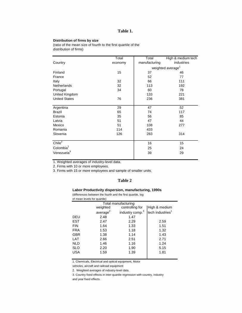
Table 1.

Distribution of firms by size(ratio of the mean size of fourth to the first quartile of thedistribution of firms)

Country Total

economy Total

manufacturing High & medium tech

industries

Finland 15 37 46France 52 77Italy 32 66 111Netherlands 32 113 192Portugal 34 60 78United Kingdom 133 221United States 76 236 381

Argentina 29 47 52Brazil 65 74 117Estonia 35 56 85Latvia 51 47 44Mexico 51 108 277Romania 114 433Slovenia 126 283 314

Chile2 16 15Colombia2 25 24Venezuela3 39 29

1. Weighted averages of industry-level data.2. Firms with 10 or more employees.3. Firms with 15 or more employees and sample of smaller units.

weighted average1

Table 2

Labor Productivity dispersion, manufacturing, 1990s(differences between the fourth and the first quartile, logof mean levels for quartile)

weighted average2

controlling for industry comp.3

High & medium tech industries1

DEU 2.48 1.47EST 2.47 2.29 2.59FIN 1.64 1.33 1.51FRA 1.53 1.18 1.32GBR 1.38 1.14 1.43LAT 2.66 2.51 2.71NLD 1.46 1.16 1.24SLO 2.20 1.90 5.15USA 1.59 1.39 1.81

1. Chemicals, Electrical and optical equipment, Motorvehicles, aircraft and railroad equipment2. Weighted averages of industry-level data.3. Country fixed effects in inter-quartile regression with country, industryand year fixed effects.

Total manufacturing

Table 3.

STANDARD DEVIATION OF LOG LABOR PRODUCTIVITY

DEU FIN FRA NLD PRT UK USATotal manufacturing (weighted avg) 0.75 0.66 0.55 0.53 0.80 0.54 0.57 Food products, beverages and tobacco 0.95 0.83 0.75 0.78 0.92 0.73 0.74 Textiles, textile products, leather and footwear 0.75 0.60 0.69 0.60 0.82 0.56 0.75 Wood and products of wood and cork 0.72 0.63 0.50 0.36 0.82 0.53 0.57 Pulp paper, paper products, printing and publishing 0.85 0.71 0.52 0.45 0.71 0.52 0.53 Coke refined petroleum products and nuclear fuel 1.10 0.54 0.96 1.02 0.95 Pharmaceuticals 0.68 0.57 0.54 0.86 0.50 0.62 Chemicals excluding pharmaceuticals 0.78 0.55 0.54 1.01 0.60 0.62 Rubber and plastics products 0.44 0.50 0.47 0.44 0.72 0.48 0.50 Other non-metallic mineral products 0.57 0.67 0.55 0.51 0.76 0.65 0.58 Basic metals 0.79 0.58 0.80 0.66 0.65 Fabricated metal products except machinery and equipment 0.47 0.43 0.68 0.45 0.50 Machinery and equipment n.e.c. 0.57 0.44 0.41 0.72 0.45 0.47 Office accounting and computing 0.90 0.48 0.87 0.61 0.72 Electrical machinery and apparatus nec 0.56 0.46 0.47 0.79 0.45 0.53 Radio, television and communication equipment 0.92 0.54 0.46 0.89 0.55 0.65 Medical precision and optical instruments 0.39 0.49 0.49 0.71 0.45 0.49 Motor vehicles, trailers and semi-trailers 0.37 0.46 0.41 0.74 0.46 0.52 Building and repairing of ships and boats 0.54 0.53 0.75 0.41 0.46 Railroad equipment and transport 0.40 0.47 0.62 0.52 0.48 Aircraft and spacecraft 0.38 0.26 0.44 0.48 Manufacturing, nec 0.50 0.62 0.49 0.44 0.86 0.50 0.50

Table 3 (continued)

STANDARD DEVIATION OF LOG LABOR PRODUCTIVITY

ARG BRA CHI COL VEN EST LAT ROM SLN KOR IND TWNTotal manufacturing (weighted avg) 0.89 1.00 0.81 0.88 0.98 0.89 1.03 1.06 0.77 0.73 1.07 0.74 Food products, beverages and tobacco 0.95 1.02 0.86 1.02 1.06 0.97 0.96 1.11 0.72 0.93 1.21 0.81 Textiles, textile products, leather and footwear 0.90 1.01 0.71 0.81 0.86 0.82 1.07 1.06 0.79 0.76 1.01 0.80 Wood and products of wood and cork 0.89 0.94 0.77 0.76 0.86 0.90 1.03 1.13 0.80 0.70 1.00 0.69 Pulp paper, paper products, printing and publishing 0.79 0.96 0.83 0.81 1.01 0.86 1.04 1.09 0.67 0.73 1.05 0.68 Coke refined petroleum products and nuclear fuel 1.11 1.01 1.55 0.96 1.23 1.03 0.41 1.02 Pharmaceuticals 0.84 0.98 0.63 0.85 0.78 1.18 1.15 0.77 0.93 1.25 0.82 Chemicals excluding pharmaceuticals 0.98 0.98 0.82 0.94 1.05 1.10 1.13 1.10 0.78 0.83 1.41 0.87 Rubber and plastics products 0.80 1.01 0.70 0.80 0.77 0.85 1.09 1.14 0.74 0.65 1.13 0.72 Other non-metallic mineral products 0.82 0.96 0.93 0.94 0.97 0.99 1.09 1.03 0.72 0.77 1.00 0.72 Basic metals 0.86 0.97 1.21 1.10 1.10 0.14 1.53 1.19 0.70 0.81 1.18 0.85 Fabricated metal products except machinery and equipment 0.86 1.07 0.76 0.77 0.89 0.87 1.01 1.07 0.77 0.66 1.05 0.68 Machinery and equipment n.e.c. 0.87 0.97 0.70 0.75 0.91 1.12 1.11 0.92 0.79 0.59 1.14 0.70 Office accounting and computing 1.04 0.46 0.59 1.09 1.14 1.20 0.72 0.79 0.75 Electrical machinery and apparatus nec 0.77 1.05 0.78 0.83 0.92 1.17 0.90 1.03 0.75 0.69 1.15 0.74 Radio, television and communication equipment 1.02 0.99 0.90 0.81 0.29 0.93 1.23 1.33 0.79 1.11 Medical precision and optical instruments 0.74 1.05 0.51 0.75 1.01 0.95 0.97 1.12 0.77 0.66 0.71 Motor vehicles, trailers and semi-trailers 0.78 0.95 0.76 0.88 0.96 0.61 1.29 0.85 0.92 0.62 1.06 0.71 Building and repairing of ships and boats 1.12 1.05 1.02 0.95 0.62 0.93 0.78 Railroad equipment and transport 1.00 1.08 0.68 0.92 0.73 1.14 0.78 Aircraft and spacecraft 0.92 1.12 1.26 Manufacturing, nec 0.74 0.99 0.75 0.76 0.86 0.77 0.86 1.12 0.75 0.68 0.75 0.72

Table 4.

STANDARD DEVIATION OF MFP

FIN FRA NLD UK USATotal manufacturing 1.77 0.20 0.15 0.19 0.34 Food products, beverages and tobacco 1.92 0.18 0.15 0.20 0.34 Textiles, textile products, leather and footwear 1.80 0.34 0.17 0.19 0.49 Wood and products of wood and cork 1.84 0.17 0.12 0.19 0.37 Pulp paper, paper products, printing and publishing 2.11 0.21 0.14 0.24 0.39 Coke refined petroleum products and nuclear fuel 2.30 0.09 0.13 0.27 Pharmaceuticals 1.87 0.24 0.17 0.25 0.37 Chemicals excluding pharmaceuticals 1.79 0.18 0.15 0.22 0.34 Rubber and plastics products 1.65 0.13 0.14 0.17 0.32 Other non-metallic mineral products 1.54 0.19 0.17 0.22 0.32 Basic metals 2.16 0.10 0.18 0.34 Fabricated metal products except machinery and equipment 1.56 0.15 0.20 0.35 Machinery and equipment n.e.c. 1.62 0.14 0.14 0.19 0.37 Office accounting and computing 1.58 0.16 0.24 0.47 Electrical machinery and apparatus nec 1.90 0.16 0.16 0.18 0.31 Radio, television and communication equipment 1.81 0.19 0.18 0.21 0.44 Medical precision and optical instruments 1.75 0.18 0.17 0.20 0.33 Motor vehicles, trailers and semi-trailers 1.68 0.30 0.11 0.18 0.30 Building and repairing of ships and boats 2.31 0.13 0.23 0.32 Railroad equipment and transport 1.81 0.12 0.21 0.25 Aircraft and spacecraft 0.16 0.19 0.29 Manufacturing, nec 1.55 0.20 0.16 0.20 0.33

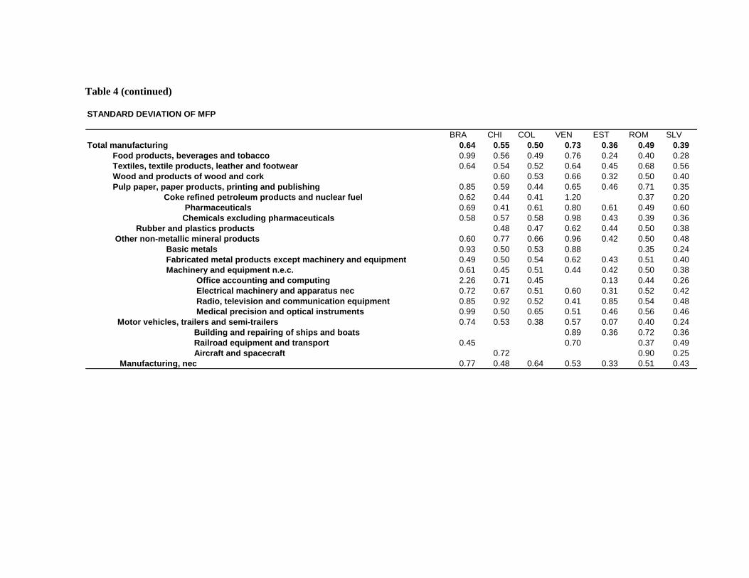
Table 4 (continued)

STANDARD DEVIATION OF MFP

BRA CHI COL VEN EST ROM SLVTotal manufacturing 0.64 0.55 0.50 0.73 0.36 0.49 0.39 Food products, beverages and tobacco 0.99 0.56 0.49 0.76 0.24 0.40 0.28 Textiles, textile products, leather and footwear 0.64 0.54 0.52 0.64 0.45 0.68 0.56 Wood and products of wood and cork 0.60 0.53 0.66 0.32 0.50 0.40 Pulp paper, paper products, printing and publishing 0.85 0.59 0.44 0.65 0.46 0.71 0.35 Coke refined petroleum products and nuclear fuel 0.62 0.44 0.41 1.20 0.37 0.20 Pharmaceuticals 0.69 0.41 0.61 0.80 0.61 0.49 0.60 Chemicals excluding pharmaceuticals 0.58 0.57 0.58 0.98 0.43 0.39 0.36 Rubber and plastics products 0.48 0.47 0.62 0.44 0.50 0.38 Other non-metallic mineral products 0.60 0.77 0.66 0.96 0.42 0.50 0.48 Basic metals 0.93 0.50 0.53 0.88 0.35 0.24 Fabricated metal products except machinery and equipment 0.49 0.50 0.54 0.62 0.43 0.51 0.40 Machinery and equipment n.e.c. 0.61 0.45 0.51 0.44 0.42 0.50 0.38 Office accounting and computing 2.26 0.71 0.45 0.13 0.44 0.26 Electrical machinery and apparatus nec 0.72 0.67 0.51 0.60 0.31 0.52 0.42 Radio, television and communication equipment 0.85 0.92 0.52 0.41 0.85 0.54 0.48 Medical precision and optical instruments 0.99 0.50 0.65 0.51 0.46 0.56 0.46 Motor vehicles, trailers and semi-trailers 0.74 0.53 0.38 0.57 0.07 0.40 0.24 Building and repairing of ships and boats 0.89 0.36 0.72 0.36 Railroad equipment and transport 0.45 0.70 0.37 0.49 Aircraft and spacecraft 0.72 0.90 0.25 Manufacturing, nec 0.77 0.48 0.64 0.53 0.33 0.51 0.43

Table 5. Calibration Statistics

Case Mean (τ)

Mean (κ)

Corr ( τ or κ ,log(A)

Mean (log(LP))

Std (log(LP))

OP cross term

(log(LP))

Mean (log(A))

Std (log(A))

OP cross term

(log(A))

Avg(K/L) Diff log(cons)

Fraction survive

No distortion 0.00 0.00 0.00 12.05 0.06 0.05 10.72 0.27 0.43 114184 0.00 0.77 Random output distortion

-0.48 0.00 0.49 12.15 0.25 -0.15 10.74 0.30 0.38 180224 -0.35 0.44

Random capital distortion

0.00 -0.05 0.10 12.14 0.06 0.05 10.74 0.26 0.42 453316 -0.63 0.72

Correlated output distortion

-0.37 0.00 0.67 11.72 0.35 -0.10 10.49 0.32 0.16 108946 -0.58 0.64

Note: All reported statistics are at steady state equilibrium reflecting selection. The reported means and standard deviations are unweighted. The OP cross term using labor productivity uses the labor input as the weight and the OP cross term using TFP (log(A)) uses the composite input as the weight.

Figure 1. Comparison of dispersion of labor and MFP productivity -- manufacturing, 1990s

(standard deviation in log productivity)

0

0.2

0.4

0.6

0.8

1

1.2

0 0.2 0.4 0.6 0.8 1 1.2

SD of labor productivity

SD o

f MFP

45'

Figure 2.

Allocative efficiency (Olley Pakes decomposition -- cross term)(weighted averages of industry level cross terms from OP decomposition)

1. Based on the three-year differences

Allocative efficiency OP cross term

-0.1

0

0.1

0.2

0.3

0.4

0.5

0.6

0.7

Argenti

naChil

e

Colombia

German

y

United

Kingdo

m

Netherl

ands

France

Finlan

d

Portug

al

United

States

Taiwan

(Chin

a)

Korea

Indon

esia(

1)

Roman

ia(1)

Sloven

iaLa

tvia

Hunga

ry

Estonia

Diff

eren

ce b

etw

een

wei

ghte

d an

d un

wei

ghte

d la

bor p

rodu

ctiv

ity

Figure 3.

Evolution of allocative efficiency during the transition -- Eastern Europe, manufacturing(weighted averages of industry level cross terms from OP decomposition)

-0.2 -0.1 0 0.1 0.2 0.3 0.4 0.5

00-01

95-96

98-99

95-96

98-99

95-96

00-01

95-96

92-93

00-01

95-96E

ston

iaLa

tvia

Rom

ania

Slo

veni

aH

unga

ry

cros

s-te

rm o

f OP

deco

mpo

sitio

n

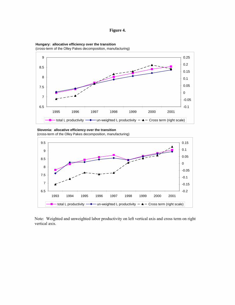
Figure 4.

Hungary: allocative efficiency over the transition(cross-term of the Olley Pakes decomposition, manufacturing)

6.5

7

7.5

8

8.5

9

1995 1996 1997 1998 1999 2000 2001-0.1

-0.05

0

0.05

0.1

0.15

0.2

0.25

total L productivity un-weighted L productivity Cross term (right scale)

Slovenia: allocative efficiency over the transition(cross-term of the Olley Pakes decomposition, manufacturing)

6.5

7

7.5

8

8.5

9

9.5

1993 1994 1995 1996 1997 1998 1999 2000 2001-0.2

-0.15

-0.1

-0.05

0

0.05

0.1

0.15

total L productivity un-weighted L productivity Cross term (right scale)

Note: Weighted and unweighted labor productivity on left vertical axis and cross term on right vertical axis.

Figure 5 The Relationship Between Productivity and Employment

No distortion Case

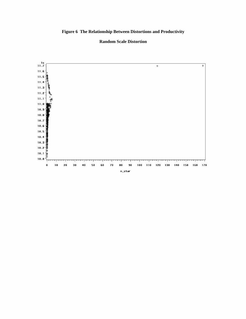
Figure 6 The Relationship Between Distortions and Productivity

Random Scale Distortion

Figure 7 The Relationship Between Distortions and Productivity

Random Factor Mix Distortion

Figure 8 The Relationship Between Distortions and Labor Productivity

Correlated Scale Distortion Case

Annex Table 1

Distribution of firms by size -- Industry level data -- manufacturing(ratio of the mean size of fourth to the first quartile of the distribution of firms)

FIN FRA GBR ITA NLD PRT USATotal manufacturing (weighted average) 37.3 52.0 133.0 66.0 113.3 60.1 236.3 Food products, beverages and tobacco 30.3 18.6 123.0 32.6 59.8 36.6 247.2 Textiles, textile products, leather and footwear 28.8 38.2 68.8 26.7 35.2 48.6 123.7 Wood and products of wood and cork 22.7 13.8 38.9 16.6 28.4 24.3 42.0 Pulp paper, paper products, printing and publishing 29.8 32.2 70.5 44.4 51.8 28.6 101.4 Coke refined petroleum products and nuclear fuel 67.0 327.6 421.7 183.6 542.9 2877.2 853.8 Pharmaceuticals 40.5 56.5 466.2 181.2 377.5 51.8 Chemicals excluding pharmaceuticals 48.6 67.9 197.6 103.9 309.0 62.7 Rubber and plastics products 27.7 30.6 99.7 40.8 79.1 29.1 112.0 Other non-metallic mineral products 30.2 33.6 127.5 47.9 75.1 37.1 79.3 Basic metals 113.8 134.1 94.7 325.3 59.5 210.2 Fabricated metal products except machinery and equipment 19.1 50.6 27.7 51.0 29.1 63.5 Machinery and equipment n.e.c. 39.9 55.1 82.1 39.0 74.8 29.1 87.6 Office accounting and computing 97.0 174.8 105.3 73.0 67.2 421.5 Electrical machinery and apparatus nec 49.9 82.2 141.0 46.0 72.7 87.2 180.4 Radio, television and communication equipment 60.7 87.3 196.2 83.6 337.9 216.0 144.8 Medical precision and optical instruments 26.4 38.1 140.8 31.8 47.2 53.7 193.4 Motor vehicles, trailers and semi-trailers 47.7 129.0 310.3 351.0 120.1 75.4 464.5 Building and repairing of ships and boats 65.8 173.7 103.2 44.6 106.5 221.4 Railroad equipment and transport 51.0 374.7 109.7 87.8 86.6 233.9 Aircraft and spacecraft 137.6 778.8 850.5 582.6 250.2 1271.8

19.7 35.3 44.2 31.4 98.6 21.6 76.7

Distribution of firms by size -- Industry level data -- manufacturing(ratio of the mean size of fourth to the first quartile of the distribution of firms)

USA ARG BRA EST IND HUN LAT MEX ROMTotal manufacturing (weighted average) 236.3 47.1 74.3 55.9 29.2 246.8 47.1 107.9 433.3 Food products, beverages and tobacco 247.2 59.6 81.1 55.3 20.2 133.6 65.5 74.7 Textiles, textile products, leather and footwear 123.7 31.9 55.2 55.3 41.1 117.0 45.7 81.9 Wood and products of wood and cork 42.0 20.8 36.1 25.6 35.7 51.3 44.6 53.1 Pulp paper, paper products, printing and publishing 101.4 42.5 53.2 31.3 21.7 58.9 46.0 58.4 213.7 Coke refined petroleum products and nuclear fuel 853.8 168.4 156.7 25.0 6.0 5272.5 5.6 38.3 228.5 Pharmaceuticals 49.3 145.0 59.5 16.9 552.4 7.9 123.0 315.6 Chemicals excluding pharmaceuticals 98.0 100.2 137.2 21.7 168.1 39.8 98.2 548.4 Rubber and plastics products 112.0 26.9 56.8 24.8 23.6 66.8 25.6 63.8 129.0 Other non-metallic mineral products 79.3 47.3 38.9 55.7 13.3 105.4 38.7 84.1 375.9 Basic metals 210.2 61.5 118.6 37.8 20.0 246.3 24.6 149.7 1213.2 Fabricated metal products except machinery and equipment 63.5 20.7 37.6 26.3 18.1 55.0 38.5 47.7 144.3 Machinery and equipment n.e.c. 87.6 27.3 73.5 45.2 18.8 74.7 47.1 854.5 Office accounting and computing 421.5 19.2 123.5 13.9 74.6 41.5 61.2 Electrical machinery and apparatus nec 180.4 34.1 97.4 83.3 20.9 183.7 21.3 672.8 Radio, television and communication equipment 144.8 74.0 136.2 139.6 29.2 187.5 46.9 378.6 Medical precision and optical instruments 193.4 25.1 73.2 39.0 55.4 64.8 58.5 337.0 Motor vehicles, trailers and semi-trailers 464.5 60.9 183.9 52.2 23.2 253.5 13.8 405.7 1053.0 Building and repairing of ships and boats 221.4 16.8 48.8 114.2 29.0 39.9 23.0 56.6 504.9 Railroad equipment and transport 233.9 27.9 96.5 58.5 23.0 127.7 14.1 176.1 1061.0 Aircraft and spacecraft 1271.8 125.7 191.7 150.7 16.0 417.6 447.9

76.7 16.6 34.4 73.2 20.9 65.8 25.6 51.5 209.1