preference construction for database querying
TRANSCRIPT

PREFERENCE CONSTRUCTION FOR DATABASE QUERYING
by
Denis Mindolin
A dissertation
submitted to the Faculty of the Graduate School
of State University of New York at Buffalo
in partial fulfillment of the requirements
for the degree of Doctor of Philosophy
Department of Computer Science and Engineering
May, 2009
Acknowledgments
It is difficult to overstate my gratitude to my PhD supervisor, Dr. Jan Chomicki. With
his enthusiasm, his inspiration, and his great efforts to explain things clearly and simply,
he helped to make my research work fun for me. Throughout my thesis-writing period,
he provided encouragement, sound advice, good teaching, and lots of good ideas. He
consistently allowed this thesis to be my own work, but steered me in the right direction
whenever he thought I needed it.
Besides my advisor, I would like to thank the rest of my thesis committee: Dr. Stuart
Shapiro and Dr. Michalis Petropoulos, for their encouragement, insightful comments, and
hard questions.
My parents, Tatyana and Sergey Mindolin, have been a constant source of support – emo-
tional, moral and of course financial – during my postgraduate years, and this thesis would
certainly not have existed without them. It is thanks to my parents that I first became
interested in science, and it is to them that this thesis is dedicated.
One of the most important persons who has been with me in every moment of my PhD
work is my wife Sveta. I would like to thank her for the many sacrifices she has made to
support me in undertaking my doctoral studies. By providing her steadfast support in hard
times, she has shown the true affection and dedication she has always had towards me.
This research has been supported by NSF Grant IIS-0307434.
ii
Contents
Acknowledgments ii
Abstract vi
1 Introduction 1
1.1 Motivation . . . . . . . . . . . . . . . . . . . . . . . . . . . . . . . . . . . 1
1.2 Binary relation preference framework . . . . . . . . . . . . . . . . . . . . 4
1.3 Our contributions . . . . . . . . . . . . . . . . . . . . . . . . . . . . . . . 6
2 Preliminaries 11
2.1 Relations and graphs . . . . . . . . . . . . . . . . . . . . . . . . . . . . . 11
2.2 Relational model . . . . . . . . . . . . . . . . . . . . . . . . . . . . . . . 13
3 p-skyline framework 15
3.1 Skyline framework . . . . . . . . . . . . . . . . . . . . . . . . . . . . . . 15
3.2 Preference constructor framework . . . . . . . . . . . . . . . . . . . . . . 16
3.3 p-skyline relations . . . . . . . . . . . . . . . . . . . . . . . . . . . . . . . 19
3.4 Attribute importance in p-skyline relations . . . . . . . . . . . . . . . . . . 25
3.5 Properties of p-skyline relations . . . . . . . . . . . . . . . . . . . . . . . 34
3.6 Minimal extensions of p-skyline relations . . . . . . . . . . . . . . . . . . 41
iii

3.7 p-skyline query evaluation . . . . . . . . . . . . . . . . . . . . . . . . . . 49
3.8 Related work . . . . . . . . . . . . . . . . . . . . . . . . . . . . . . . . . 51
4 Discovery of p-skyline relations 55
4.1 Feedback based discovery of p-skyline relations . . . . . . . . . . . . . . . 55
4.2 Constraints to discover p-skyline relations . . . . . . . . . . . . . . . . . . 59
4.3 Using superior/inferior examples for p-skyline discovery . . . . . . . . . . 61
4.4 Using only superior examples for p-skyline discovery . . . . . . . . . . . . 68
4.5 Experiments . . . . . . . . . . . . . . . . . . . . . . . . . . . . . . . . . . 87
4.6 Related work . . . . . . . . . . . . . . . . . . . . . . . . . . . . . . . . . 95
5 Hierarchical CP-nets 99
5.1 CP-network framework . . . . . . . . . . . . . . . . . . . . . . . . . . . . 99
5.2 HCP-nets . . . . . . . . . . . . . . . . . . . . . . . . . . . . . . . . . . . 104
5.3 Dominance testing for HCP-nets . . . . . . . . . . . . . . . . . . . . . . . 110
5.4 Formula representations of HCP-nets . . . . . . . . . . . . . . . . . . . . . 113
5.5 Experimental evaluation . . . . . . . . . . . . . . . . . . . . . . . . . . . 115
5.6 Related work . . . . . . . . . . . . . . . . . . . . . . . . . . . . . . . . . 121
6 Preference contraction 124
6.1 Requirements to preference contraction . . . . . . . . . . . . . . . . . . . 124
6.2 Scenario of minimal preference contraction . . . . . . . . . . . . . . . . . 127
6.3 Preference contraction in binary relation framework . . . . . . . . . . . . . 129
6.4 Properties of full contractors . . . . . . . . . . . . . . . . . . . . . . . . . 130
6.5 Construction of a minimal full contractor . . . . . . . . . . . . . . . . . . 138
6.6 Contraction by finitely stratifiable relations . . . . . . . . . . . . . . . . . 143
6.7 Preference-protecting contraction . . . . . . . . . . . . . . . . . . . . . . . 150
6.8 Meet preference contraction . . . . . . . . . . . . . . . . . . . . . . . . . 155
6.9 Querying with contracted preferences . . . . . . . . . . . . . . . . . . . . 161
6.10 Experimental evaluation . . . . . . . . . . . . . . . . . . . . . . . . . . . 163
iv

6.11 Related work . . . . . . . . . . . . . . . . . . . . . . . . . . . . . . . . . 168
7 Conclusions and future work 178
7.1 Preference specification . . . . . . . . . . . . . . . . . . . . . . . . . . . . 178
7.2 Preference discovery . . . . . . . . . . . . . . . . . . . . . . . . . . . . . 182
7.3 Preference change . . . . . . . . . . . . . . . . . . . . . . . . . . . . . . . 185
References 188
A Omitted proofs 198
v

Abstract
In this dissertation, we develop methods of constructing preferences in the binary relation
preference framework. This framework has been introduced recently to allow querying
databases using preferences. Preferences here are strict partial order binary relations over
objects. The framework allows for finite and infinite preference relations (represented as
finite formulas).
Having a high expressive power, the binary relation framework lacks simple user- ori-
ented methods of constructing preferences. Therefore, special query interfaces need to be
developed to simplify the process of building preferences. In order to make preference
construction easier, we pursue the following research directions.
First, we study the problem of attribute importance in preference relations. We propose
a class of preference relations called p-skylines which extend widely used skyline prefer-
ence relations with the notion of attribute importance. We show that attribute importance in
p-skylines can be captured as graphs. We study properties of p-skyline relations and show
methods of checking containment and dominance testing in this framework. We introduce
an algorithm of computing minimal extensions of p-skyline relations.
Second, we propose to use the sets of the most preferred and the most unpreferred
objects to discover importance of attributes in the underlying p-skyline relations. We study
the complexity of the discovery problem and show an efficient algorithm for discovery of
p-skyline relations given sets of most preferred objects.
vi
vii
Third, we propose to view a variant of the CP-net framework to construct preferences as
preference relations. CP-nets is a well established graphical model of preference specifica-
tion, widely used in AI. We introduce an original variant of CP-nets, which allows to work
with infinite domains. We develop an algorithm of constructing polynomial-size formulas
representing the relations induced by given CP-net instances.
Fourth, we develop a method of constructing preference relations by discarding subsets
of existing preference relations. Discarding preferences is a common way of changing
preferences in real life. The operation of preference contraction we develop here allows
for contracting finite and infinite preference relations represented as formulas. We propose
several variants of the preference contraction operator, study their properties, and introduce
algorithms for their evaluation.

Chapter 1Introduction
1.1 Motivation
User preference management is an essential part of any modern business. Knowing what
customers like, why they like it, and more importantly what they will like in the future al-
lows for efficient production planning, inventory stocking, and enhanced profitability. Most
modern businesses use databases to store inventory related information, and the amounts
of data stored grow rapidly. Thus, there is a need of efficient querying such databases with
preferences.
In order to incorporate preferences into existing database query languages, the binary
relation preference framework has been introduced independently by Kießling [Kie02] and
Chomicki [Cho03]. Preferences here are binary relations over objects. They are required
to be strict partial orders (SPO): transitive and irreflexive binary relations. This framework
can deal with finite as well as infinite preference relations, the latter represented using finite
first order formulas which are called preference formulas.
EXAMPLE 1.1 Suppose Mary wants to buy a car and her preference over cars is that
she prefers newer cars and among the cars made in the same year, the cheaper one is
1

CHAPTER 1. INTRODUCTION 2
preferable. This preference can be represented as the following preference formula.
o1 o2 ≡ o1.year > o2.year∨o1.year = o2.year∧o1.price < o2.price
The expression above represents the fact that the car o1 is preferred to the car o2 iff the
formula evaluates to true.
A special relational algebra operator called winnow [Cho03] (called BMO in [Kie02]) is
used to compute sets of the most preferred objects in a database relation given a preference
formula. An extension of SQL has been proposed to allow querying relational databases
with preferences represented as binary relations [KK02].
Dealing with preferences in this framework, many existing works assume that prefer-
ence relations are provided for such queries directly by users. However, such scenarios are
far from being realistic, and it is hard to expect that a user can easily represent his or her
preference as a preference relation. We see the following challenges here.
The first issue is that in many scenarios, formulating preferences directly by target users
is impossible or hard to achieve. One reason is that a process of preference construction
may take a long time which is often unacceptable. Another reason is that a user may be not
clear about his or her own preferences. In such cases, preference discovery becomes useful.
It is intended to construct an accurate model of user’s preference, find hidden preferences,
and avoid redundancy.
An important part of preference discovery is discovery of attribute importance. An
attribute A is generally considered more important than another attribute B if when ob-
jects are compared by A, their values of B do not matter or matter less. In order to be
able to discover the importance relationship of attributes, the preference framework has
to support this notion. One class of preference relations to which this notion applies is
skyline preference relations [BKS01]. Any such a preference relation induces equal impor-
tance of attributes. Another class of preference relations in which the notion of attribute

CHAPTER 1. INTRODUCTION 3
importance is present is considered in the preference constructor framework [Kie04]. How-
ever, importance here is considered on the level of (possibly complex) preference relations
composed in another relation. The problem of importance of attributes induced by such
preference relations has not been studied yet. Even though a number of methods have
been proposed for discovering preference relations of these classes based on user feedback
[HEK03, JPL+08, LwYwH+08], none of them addresses discovery of attribute importance.
The second challenge is that preference relations may be rather complex. Thus, even
if one has a full picture of his or her preferences in mind, it may be hard for him or her to
formulate the preferences as a preference relation. Similar problem has been address in the
method of constructing preferences called CP-networks [BBHP99]. Preferences here are
defined using graphs in which every node is an attribute, and an edge from one attribute to
another implies that the preference over the second attribute is conditioned on the values
of the first attribute. Such conditions are expressed in the form of conditional preference
tables (CPT) associated with every node of graph. This model exploits the ceteris paribus
principle: given a CPT, one object is preferred to another if 1) both objects satisfy the
CPT condition, 2) the first object is preferred to the second object via the CPT preference
order, and 3) everything else is equal. The preference relations induced by some classes
of CP-networks [BBD+04] are strict partial orders. The CP-network approach is generally
used outside of the scope of the binary relation model. Namely, the domains here are
considered to be finite, and ad hoc algorithms are used to work with different classes of CP-
networks. Some attempts have been performed to adapt CP-networks to the binary relation
framework. [CS05, EK06] proposed an approach of constructing preference formulas for
CP-networks. However, formulas constructed here are of exponential size in general.
The third issue is that in many cases, construction of preferences is an iterative pro-
cess of their change. However, requiring a user to reconstruct the preference relation from
scratch each time she changes her mind is unrealistic for practical reasons. In such sce-

CHAPTER 1. INTRODUCTION 4
narios, it is more natural to change preference relations step-by-step by changing only the
pieces which need to be altered. Several preference change operations have been intro-
duced in this framework: preference revision[Cho07b] and equivalence adding[BGS06].
However, these operations are limited since they allow only semantical adding new pref-
erences and equivalences to existing preferences. At the same time, it is very common to
discard some preferences one used to hold if the reasons for holding those preferences are
no longer valid. This kind of change cannot be represented by any of the operations above.
1.2 Binary relation preference framework
In this section, we formally define a variant of the binary relation preference framework
which is the scope of the current work. It is a simple and at the same time a general
framework of querying databases with preferences.
Let A = A1, ...,An be a finite set of attributes. Let every attribute Ai ∈A be associated
with an infinite domain DAi . The domains considered here are rationals Q and uninterpreted
constants (numerical or categorical) C .
Let the universe of tuples U be defined as ∏Ai∈A DAi . Given a subset S of A , we denote
∏Ai∈S DAi as US. Given a tuple o ∈US for some S ⊆ A , we denote the value of the Ai ∈ S
of o as o.Ai. For two sets of attributes S1 and S2 such that S1 ⊆ S2 ⊆A , and a tuple o∈US2 ,
the tuple obtained from o by leaving only the values of S1 in it is denoted as o.S1.
Given a set of attributes S ⊆ A , we denote the set of pairs of tuples from U which are
equal in every attribute in S as ≈S, i.e.
≈S= (o,o′) | o,o′ ∈U ∧∀A ∈ S . o.A = o′.A.
Preferences in this framework are represented as binary relations over tuples.

CHAPTER 1. INTRODUCTION 5
DEFINITION 1.1 [Cho03] Given a relation schema R(A1, . . . ,An), a relation is a
preference relation over R if it is a subset of U×U and a strict partial order (SPO).
Binary relations considered in the framework are finite or infinite. Finite binary relations
are represented as sets of pairs of tuples. The infinite binary relations we consider here are
finitely representable as formulas. Given a binary relation R, its formula representation is
denoted FR. The formula representation F of a preference relation is called a preference
formula.
We consider two kinds of atomic formulas here:
• equality constraints: o.Ai = o′.Ai, o.Ai 6= o′.Ai, o.Ai = c, or o.Ai 6= c, where o,o′ are
tuple variables, Ai is a C -attribute, and c is an uninterpreted constant;
• rational-order constraints: o.Aiθo′.Ai or o.Aiθc, where θ ∈ =, 6=,<,>,≤,≥, o,o′
are tuple variables, Ai is a Q -attribute, and c is a rational number.
A preference formula whose all atomic formulas are equality (resp. rational-order)
constraints will be called equality (resp. rational order) preference formula. If both
equality and rational order constraints are used in a formula, the formula will be called
equality/rational order formula or simply ERO-formula. Without loss of generality, we
assume that all preference formulas are quantifier-free because ERO-formulas admit quan-
tifier elimination.
An element of a preference relation is called a preference. We use the symbol with
subscripts to refer to preference relations. We write x y as a shorthand for (x y∨ x = y).
We also say that x is preferred to y and y is dominated by x according to if x y.
The two most common operations which involve preferences are
• dominance testing, i.e. checking if one tuples dominates another according to a given
preference relation, and
CHAPTER 1. INTRODUCTION 6
• computing the best objects, i.e. computing sets the most preferred tuples in a given
relation instance, according to a given preference relation.
To solve the former problem, one needs check if the corresponding preference formula
evaluates to true for the given pair of tuples. To address the latter problem, the algebraic
operator of winnow is used in this framework. The winnow operator picks from a given
relation the set of the most preferred tuples, according to a given preference formula.
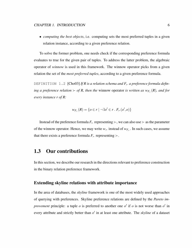
DEFINITION 1.2 [Cho03] If R is a relation schema and F a preference formula defin-
ing a preference relation of R, then the winnow operator is written as wF(R), and for
every instance r of R:
wF(R) = o ∈ r | ¬∃o′ ∈ r . F(o′,o)
Instead of the preference formula F representing, we can also use as the parameter
of the winnow operator. Hence, we may write w instead of wF . In such cases, we assume
that there exists a preference formula F representing .
1.3 Our contributions
In this section, we describe our research in the directions relevant to preference construction
in the binary relation preference framework.
Extending skyline relations with attribute importance
In the area of databases, the skyline framework is one of the most widely used approaches
of querying with preferences. Skyline preference relations are defined by the Pareto im-
provement principle: a tuple o is preferred to another one o′ if o is not worse than o′ in
every attribute and strictly better than o′ in at least one attribute. The skyline of a dataset
CHAPTER 1. INTRODUCTION 7
is the set of the most preferred tuples according to the skyline preference relation. A well
known property of skyline relations is that they induce equal importance of attributes.
In Chapter 3, we develop the p-skyline framework which generalizes the skyline frame-
work by enriching it with the notion of variable attribute importance. Similarly to a sky-
line preference relation, a p-skyline preference relation is composed of preferences over
attributes (also called atomic preferences). Every p-skyline relation is characterized by a p-
graph which captures the difference in the importance of attributes induced by the relation.
Nodes of such graphs are attributes, and edges go from more to less important attributes. A
skyline preference relation is a p-skyline relation whose p-graph has no edges.
We identify the class of full p-skyline relations, i.e., p-skyline relations which are com-
posed of all atomic preferences relations in a given set. We study properties of such rela-
tions. First, we show a necessary and sufficient condition for a graph to be a p-graph of
a p-skyline relation. Second, we study the problems of containment and equivalence of
full p-skyline relations and show that they may be reduced to simple problems of checking
containment and equivalence of their p-graphs. Third, we investigate the problem of testing
dominance in this framework and propose several efficient methods to solve that problem.
The next problem we explore is computing minimal extensions of full p-skyline rela-
tions. We show that given a p-skyline relation, there exists at most polynomial number
of full p-skyline relations minimally extending it, all computable in polynomial time. To
compute all such minimal extensions, we propose a set of simple rewriting rules which are
applied to the syntax tree of a p-skyline relation.
Last, we show that preference queries in this framework may be evaluated efficiently. In
particular, we show how the existing methods of skyline query evaluation may be adapted
in this framework.

CHAPTER 1. INTRODUCTION 8
Feedback-based discovery of attribute importance
In Chapter 4, we study the problem of discovering user preferences in the form of p-skyline
relations based on user feedback. As feedback, we propose to use sets of superior examples
G (i.e, the tuples which a user likes) and inferior examples W (i.e., the tuples which a user
dislikes) in a given data set O. A p-skyline relation according to which tuples in G are
among the best and tuples in W are not among the best in O is called favoring G/disfavoring
W in O. A maximal p-skyline relation favoring G/disfavoring W is called optimal.
First, we show that the problem of existence of a favoring/disfavoring p-skyline re-
lation is NP-complete in general. Second, we prove that the problem of computing any
favoring/disfavoring p-skyline relation (even an optimal one) is in general FNP-complete.
Next, we study restricted versions of these problems in which sets of inferior examples
W are empty. We show that the problem of existence of a favoring p-skyline relation can
be solved in polynomial time and may be reduced to evaluation of the skyline operator.
Second, we show that the problem of computing an optimal p-skyline relation can be solved
by computing a p-graph satisfying a system of constraints called negative. We develop an
efficient polynomial time algorithm for constructing such p-skyline relations. To reduce
the number of constrains used by the algorithm and hence improve its running time, we
propose a set of optimization techniques. The results of experimental evaluation of the
proposed algorithms are also provided in this chapter.
Graphical model to represent preference relations
In Chapter 5, we introduce a variant of the CP-net framework called HCP-nets. One of the
issues of CP-nets we address here is that the conditionality of preferences over attributes in
CP-nets does not always imply difference in attribute importance. At the same time, such a
relationship between atomic preferences and the corresponding attributes may by implied
by a user. It has been shown [BBD+04] that this property of CP-nets is due the strictness
CHAPTER 1. INTRODUCTION 9
of the ceteris paribus principle of comparing tuples exploited in CP-nets. In the proposed
HCP-net framework, we relax this principle by requiring that children of an attribute in a
conditional preference graph should not be considered when tuples are compared by that
attribute. As a result, all children of an attribute in a conditional preference graph are less
important.
The next deficiency of CP-nets we address in HCP-nets is the inability of CP-nets to
deal with attributes with infinite domains. Since infiniteness of domains is an important
property of the binary relation preference framework, we allow attribute domains to be
finite or infinite in HCP-nets.
We show that the HCP-net framework has a number of interesting properties. First, we
show that dominance testing in HCP-nets is in PTIME and provide several methods to solve
that problem. We note that the corresponding problem for CP-nets is in PTIME for limited
classes and NP-hard for a class of nets structurally close to HCP-nets. Second, we show
a technique of representing orders induced by HCP-nets as polynomial size preference
formulas. Last, we evaluate the proposed methods and study their scalability and running
time with respect to the corresponding algorithms for CP-nets.
Constructing preference relations by discarding their subsets
In Chapter 6, we investigate the problem of constructing preference relations by changing
them. In particular, we consider the operation of preference contraction – discarding a
subset (called a base contractor here) of a preference relation. The preference contraction
operation we propose here has two important properties: preservation of strict partial order
properties in the modified preference relation and minimality of preference relation change.
We study preference contraction in the view of the scenario in which a user iteratively
explores alternative ways of contracting a preference relation to find the most suitable one.
We assume that a user intends to contract preferences in a minimal way in every iteration,

CHAPTER 1. INTRODUCTION 10
i.e., discard a minimal set of preferences (including the base contractor) needed to preserve
the strict partial order of the preference relation. The corresponding operator is called
minimal contraction. This operation can be constrained by the requirement of protecting
some preferences from removal (preference protecting minimal contraction). An important
property of minimal contraction is that it may be performed in many different ways. In
order to explore the effect of performing minimal contraction (preference protecting min-
imal contraction) in all possible ways and help make a decision on the way closer to the
user intentions, we propose the operation of meet contraction (meet preference protecting
contraction, respectively).
We show necessary and sufficient conditions for a subset of a preference relation to
contract it minimally. We also identify a special class of base contractors – stratifiable base
contractors. For this class, we propose a method of evaluating minimal contraction. For a
subclass of stratifiable base contractors called finitely stratifiable, we show two algorithms
for computing minimal contraction: for finite and finitely representable infinite preference
relations. A method of computing meet contraction is also provided here. Additionally,
we show methods of computing these operators in the presence of preference-protection
constraints.
We also consider the proposed contraction operators in the context of belief revision.
We show a variant of the preference state framework [Han95] in which operations of pref-
erence change may be computed using preference revision [Cho07b] and the contraction
operators proposed here. We also study properties of this framework.
Finally, we perform an experimental evaluation of the proposed contraction operators
on finite preference relations and present the results.
Chapter 2Preliminaries
In this chapter, we review the standard notions of the partial order set theory [Sch03] and
relational databases [AHV95].
2.1 Relations and graphs
We use the standard definition of binary relations. Namely, a binary relation R over a (finite
or infinite) set S is a subset of S× S. Binary relations may be finite or infinite. We write
R(x,y) or xy ∈ R to denote that (x,y) ∈ R.
Here we list some typical properties of binary relations. A binary relation R is
• irreflexive iff ∀x . ¬R(x,x),
• asymmetric iff ∀x,y . R(x,y)→¬R(y,x)
• transitive iff ∀x,y,z . R(x,y)∧R(y,z)→ R(x,z)
• negatively transitive iff ∀x,y,z . ¬R(x,y)∧¬R(y,z)→¬R(x,z)
• connected iff ∀x,y,z . R(x,y)∨R(y,x)∨ x = y
11
CHAPTER 2. PRELIMINARIES 12
• a strict partial order (SPO) if it is irreflexive and transitive;
• a weak order if it is a negatively transitive strict partial order;
• a total order if it is a connected strict partial order.
A weak order R has the following property
∀x,y,z . R(x,y)→ R(x,z)∨R(z,y)
Let the range of a binary relation R be defined as
rangeR = x | ∃y . R(x,y)∨R(y,x)
Let the transitive closure of a binary relation R be denoted as TC(R) and defined as
(x,y) ∈ TC(R) iff Rm(x,y) for some m≥ 0,
where
R1(x,y)≡ R(x,y)
Rm+1(x,y)≡ ∃z . R(x,z)∧Rm(z,y)
A finite or infinite binary relation R⊆ S×S may be viewed as a directed graph, finite or
infinite, respectively. The set S is called the nodes of R and denoted as N(R). We say that
the tuple xy is an R-edge from x to y if (x,y) ∈ R. A path in R (or an R-path) from x to y for
an R-edge xy is a sequence of R-edges such that the start node of the first edge is x, the end
node of the last edge is y, and the end node of every edge (except the last one) is the start
node of the next edge in the sequence. The length of an R-path is the number of R-edges in

CHAPTER 2. PRELIMINARIES 13
the path. An R-sequence is the sequence of nodes participating in an R-path. The length of
an R-sequence is the number of nodes in it.
Given a directed graph R and its node x,
• ChR(x) = y | (x,y) ∈ R is the set of children of x in R,
• PaR(x) = y | (y,x) ∈ R is the set of parents of x in R,
• DescR(x) = y | (x,y) ∈ TC(R) is the set of descendents of x in R,
• AncR(x) = y | (y,x) ∈ TC(R) is the set of ancestors of x in R,
• SiblR(x) = N(R)− (DescR(x)∪AncR(x)∪x) is the set of siblings of x in R
We also write Desc-sel fR(x) and Anc-sel fR(x) as shorthands of (DescR(x)∪x) and
(AncR(x)∪x), respectively.
Given two nodes x and y of R and two sets of nodes X and Y of R, we write
• R |= x∼ y iff (x,y) 6∈ R and (y,x) 6∈ R;
• R |= X ∼ Y iff ∀x ∈ X ,y ∈ Y . R |= x∼ y;
• (X ,Y ) ∈ R iff ∀x ∈ X ,y ∈ Y . (x,y) ∈ R.
2.2 Relational model
A database schema is a set of names of relations of fixed arity. Relation and attribute
names are drawn from an infinite set of names. Every attribute of a relation is associated
with a domain: rationals Q or uninterpreted constants C . Two constants are considered to
be equal if the corresponding names are the same. We use the natural interpretation of the
built-in symbols >, ≥, <, ≤, and = over decimals.

CHAPTER 2. PRELIMINARIES 14
Throughout the document, we use the relational algebra language to query relational
database instances. Queries in this language have the following grammar:
E ::= R | σθ(E) | φX(E) | E1×E2 | E1∪E2 | E1−E2 | E1 ./E1.Ai1=E2.A j1 ,...,E1.Aim=E2.A jm
E2
where R is any relation name, Ai1, . . . ,Aim ,A j1, . . . ,A jm are attribute names, σ, φ,×, ∪,−, ./
are the selection, projection, Cartesian product, union, set difference, and join operators,
respectively. The selection condition θ is a quantifier-free formula over the correspond-
ing relation, and X is a list of attributes. We evaluate relation algebra expressions in the
standard way.
Chapter 3p-skyline framework
In this chapter, we propose the p-skyline framework. It is a generalization of the skyline
approach of querying databases with preferences. Before going to details of the p-skyline
framework, we describe the two frameworks it is based on: skylines and preference con-
structors.
3.1 Skyline framework
DEFINITION 3.1 Let A be an attribute from the universe of attributes A . Then an
atomic preference relation over A is a total order >A which is a subset of DA×DA.
Given a set of atomic preference relations H = >A1, . . . ,>An for every attribute in A ,
the skyline preference relation for H is denoted as skyH . The relation skyH represents the
Pareto improvement principle. Namely, a tuple o is preferred to another tuple o′ according
to skyH if and only if
1. for every attribute Ai ∈ A , we have o.Ai >Ai o′.Ai or o.Ai = o′.Ai. In other words, o
is not worse than o′ according to every attribute, and
15

CHAPTER 3. P-SKYLINE FRAMEWORK 16
2. for some attribute Ai ∈ A , we have o.Ai >Ai o′.Ai. In other words, o is strictly pre-
ferred to o′ according to at least one attribute.
Given a set of tuples r, its skyline is the set of the most preferred tuples in r according to
skyH . In other words, the skyline of r is the result of wskyH (r). The corresponding winnow
query in the skyline framework is called the skyline query.
It is known that skyline preference relations are strict partial orders. They are repre-
sentable using preference formulas if the corresponding atomic preference relations are. A
number of optimization algorithms have been developed to compute skyline queries. We
discuss some of them in the related work.
3.2 Preference constructor framework
The preference constructor framework has been proposed in [Kie02]. Preference relations
here are strict partial order relations constructed from a fixed set of base preference con-
structors using a set of operators.
DEFINITION 3.2 Let A be an attribute in A . Then a base preference constructor is a
tuple (A,>A), where >A is a strict partial order over DA.
Various base preference constructors are defined here for categorical as well as numer-
ical domains. To construct a complex preference relation from base preference construc-
tors, the following set of operators is used: Pareto accumulation, which represents equal
importance of the preference relations being combined; prioritized accumulation, which
represents a difference in the importance of the preference relations being combined; in-
tersection and disjoint union, which are used to aggregate preference relations. Preference
relations composed recursively using these operators are called accumulational.
DEFINITION 3.3 Let Var() be the set of all relevant attributes. A relation is an
accumulational relation iff

CHAPTER 3. P-SKYLINE FRAMEWORK 17
• is induced by a base preference constructor (A,>A)
= (o,o′) | o,o′ ∈U . o.A >A o′.A.
Then Var() = A.
• is a prioritized accumulation of two accumulational relations1 and2 (denoted
as 1 & 2), defined as
≡ 1 ∪ (≈Var(1) ∩ 2) (3.1)
Then Var() = Var(1)∪Var(2).
• is a Pareto accumulation of two accumulational relations 1 and 2 (denoted as
1 ⊗ 2), defined as
≡ (1 ∩ ≈Var(2)) ∪ (2 ∩ ≈Var(1)) ∪ (1 ∩ 2) (3.2)
Then Var() = Var(1)∪Var(2).
• is an intersection of two accumulational relations 1 and 2 defined as
≡ 1 ∩ 2,
such that Var(1) = Var(2). Then Var() = Var(1) = Var(2).
• is an disjoint union of two accumulational relations 1 and 2 defined as
≡ 1 ∪ 2,
such that Var(1) = Var(2) and range1∩ range2 = /0. Then Var() = Var(1)
CHAPTER 3. P-SKYLINE FRAMEWORK 18
= Var(1).
Some properties of accumulational operators are summarized below.
PROPOSITION 3.1 [Kie02] The operators ⊗ and & are associative. The operator
⊗ is commutative.
PROPOSITION 3.2 [Kie02] An accumulational preference relation is an SPO.
Accumulational preference relations is a foundation of the Preference SQL [KK02]
language of querying databases with preferences. This language extends SQL by adding the
PREFERRING keyword which is used to embed preferences into SQL queries. Preferences
here are accumulational relations. Every base constructor has a special keyword in this
language (e.g., HIGHEST, LOWEST, AROUND). Base constructors are composed into more
complex expressions using the AND keyword, representing Pareto accumulation, and the
CASCADE keyword, representing prioritized accumulation. Below we show an example of
such a query.
SELECT * FROM P
PREFERRING HIGHEST(memory) AND HIGHEST(cpu) CASCADE
LOWEST(price)
This query is equivalent to w(P) where
≡ (memory ⊗ cpu) & price,
where memory and cpu represent the preferences that higher values of memory and cpu
are preferred, and price represents the preference that lower values of price are preferred.
CHAPTER 3. P-SKYLINE FRAMEWORK 19
3.3 p-skyline relations
The skyline framework and the preference constructor framework are among the major
approaches of querying databases with preferences. The former approach is very simple:
a user needs to provide a set of relevant attributes and atomic preferences over them to
construct a preference query. A great number of optimization algorithms have been devel-
oped for skyline queries. On the other hand, a well known limitation of this framework is
that attributes in a skyline preference relation are of the same importance. Hence, prefer-
ences with different importance of attributes cannot be represented as skyline preference
relations.
The latter framework has much richer expressive power than the skyline framework. In
this framework, preference relations composed into another preference relation may be of
the same or different importance. It has been shown [KK02] that skyline preference rela-
tions are representable in this framework. Moreover, preference queries in this framework
are representable as Preference SQL statements and can be evaluated efficiently [HK05].
An important property of the preference constructor framework that it deals with the
notion of importance on a high level. For instance, if = 1 ⊗ 2 ( = 1 & 2, re-
spectively), then the preference relation1 is known to be as important as (more important
than, respectively) 2 in . However, the same relationship may not hold between 1 and
2 after composing with another preference relation.
EXAMPLE 3.1 Consider two preference relations 1 and 2 defined as
1 ≡ A1 & A2
2 ≡ 1 ⊗ A2
According to the semantics of & , the preference relation A1 is more important than
A2 in 1 . However, despite the fact that 1 is used in construction of 2 , the same
CHAPTER 3. P-SKYLINE FRAMEWORK 20
importance relationship between A1 and A2 as in 1 does not hold in 2 . Namely,
it is easy to check that A1 and A2 are of equal importance in 2 .
Moreover, the notion of attribute importance has not been addressed in this framework:
given a preference relation, determine the importance relationship between two attributes
in the preference relation.
The focus of this chapter is to develop a preference framework
1. which generalizes the skyline framework by enriching it with the notion of attribute
importance;
2. in which attribute importance implied by a preference relation is intuitively captured;
and
3. in which preference queries can still be represented as Preference SQL statements
and evaluated efficiently.
Here we propose a framework which has all these properties. It is called the p-skyline
framework. Similarly to the skyline framework, preference relations here are composed of
atomic preference relations.
DEFINITION 3.4 Let A be an attribute from the set A with the domain DA. Then
an atomic preference relation over A is a total order >A which is a subset of DA×DA
representable as a preference formula.
To construct p-skyline relations, two operators of the preference constructor framework
are used. First, Pareto accumulation is used to represent equal importance of the composed
preference relations (1 and 2 are equally important in 1 ⊗ 2). Second, prioritized
accumulation is used to represent different importance of the composed preference relations
( 1 is more importance than 2 in 1 & 2).

CHAPTER 3. P-SKYLINE FRAMEWORK 21
DEFINITION 3.5 A preference relation is a prioritized skyline relation or simply a
p-skyline relation if one of the following holds:
1. is induced by an atomic preference relation >A ∈H (denoted as A)
≡ (o,o′) | o,o′ ∈U . o.A >A o′.A.
Then Var() = A.
2. is a prioritized accumulation (see (3.1)) of two p-skyline relations 1 and 2
(denoted as 1 & 2), where Var(1)∩Var(2) = /0. Then Var() = Var(1
)∪Var(2).
3. is a Pareto accumulation (see (3.2)) of two p-skyline relations1 and2 (denoted
as 1 ⊗ 2 ), where Var(1)∩Var(2) = /0. Then Var() = Var(1)∪Var(2).
Since accumulation operators are associative, we extend them from binary to n-ary
operators.
As in the skyline framework, let the set H of atomic preference relations contain an
atomic preference relation >A for every attribute A ∈ A . We denote the set of all p-skyline
relations, each composed from all members of H , by FH . Such relations are called full
p-skyline relations. Further we consider only full p-skyline relations. It follows from the
definition above that Var() of a full p-skyline relation is A .
A nice property of p-skyline relations is that they are SPO. This follows from [Kie02].
According to the next proposition, a p-skyline relation can be represented by a polynomial
size formula.
PROPOSITION 3.3 A p-skyline relation can be represented by a preference formula
F of size |F| = O(|Var()|2 + Lmax · |Var()|), where Lmax is the length of the longest
formula representing the members of H .

CHAPTER 3. P-SKYLINE FRAMEWORK 22
PROOF
If is induced by an atomic preference >A, then obviously |F| = O(Lmax). If =
1 & 2, then F can be written using (3.1) by replacing the sets with the corresponding
formulas and the set operators with the corresponding boolean operators. If=1 ⊗ 1,
then it can represented by the following formula
F(o,o′) =(
F1(o,o′) ∨ F≈Var(1)(o,o′))∧(
F2(o,o′) ∨ F≈Var(2)(o,o′))∧
¬F≈(Var(1)∪Var(2))(o,o′).
Note that |F≈S | = Θ(|S|) for any set of attributes S. Hence, if is a Pareto or prioritized
accumulation of 1 and 2, then
|F| ≤ |F1|+ |F2|+2 · (|Var(1)|+ |Var(1)|)+T1
for a constant T1. By induction in the size of F, it can be shown that
|F| ≤ T2 · (|Var()|2 +Lmax · |Var()|)
for T2 ≥ (2 + T12 ). Moreover, it is easy to check that a p-skyline relation whose size is
Θ(|Var()|2 +Lmax · |Var()|) may be constructed by composing atomic preference rela-
tions using only Pareto accumulation.
A key property of the p-skyline framework is that a skyline relation is a full p-skyline
relation. Recall that given a set of atomic preference relations H , skyH is a skyline relation
over the set of atomic preferences H . It can be easily checked that
skyH ≡ A1 ⊗ . . . ⊗ An ,
where A1, . . . ,An are the preference relations induced by the members >A1, . . . ,>An of

CHAPTER 3. P-SKYLINE FRAMEWORK 23
H .
We note that the p-skyline framework is defined as a restriction of the preference con-
structor framework described in Section 3.2. These frameworks have the following distinc-
tions:
1. in the preference constructor framework, the orders induced by base constructors are
SPO. The corresponding atomic preference relations in the p-skyline framework are
total orders. This allows us to keep the p-skyline framework similar to the skyline
framework, where atomic preference relations are total orders;
2. in the p-skyline framework, we use only two operators for preference relation con-
struction: Pareto accumulation and prioritized accumulation. As we show further,
they are sufficient to express variable attribute importance in p-skyline relations;
3. for every attribute, an atomic preference relation over it appears once in a p-skyline
relation. As we show further, this allows for a simple graphical method of capturing
difference in the importance of attributes induced by p-skyline relations.
3.3.1 Syntax tree representation
Dealing with p-skyline relations, it is natural to represent them as p-skyline syntax trees.
DEFINITION 3.6 A p-skyline syntax tree T of a p-skyline relation is an ordered
rooted tree representing the syntactic structure of the expression (in terms of accumulation
operators and p-skyline relations induced by atomic preference relations) defining .
Every non-leaf node of a p-skyline syntax tree is labeled with an accumulation operator and
corresponds to the result of applying the operator to the p-skyline relations represented by
its children from left to right. Every leaf node of a p-skyline syntax tree is labeled with an
attribute A ∈ A and corresponds to the p-skyline relation induced by the atomic preference

CHAPTER 3. P-SKYLINE FRAMEWORK 24
relation >A ∈ H . Given a node C of a syntax tree, we denote the i-th child node of C in
the syntax tree as C[i]. The syntax tree representation of p-skyline relations is widely used
in Section 3.6 for computing minimal extensions of a p-skyline relation.
A p-skyline syntax tree is called normalized if every non-leaf node is labeled differently
from its parent. Intuitively, a normalized p-skyline syntax tree represents the expression
representing a p-skyline relation in which all parentheses nonessential due to associativity
of ⊗ and & are removed. Clearly, for every p-skyline relation, there is a normalized p-
skyline syntax tree which may be constructed in polynomial time in the size of the original
tree. To do that, one needs to find all occurrences of syntax tree nodes C1 and their children
C2 such that C1 and C2 have the same label. After that, C2 has to be removed from the child
list of C1, and the list of children of C2 has to be added to the child list of C1 in place of C2.
This procedure is summarized in Algorithm 3.1. The function normalizeTree takes
the root node of an unnormalized tree and performs the tree normalization. Algorithm
3.1 is trivial and provided here solely for the sake of completeness. We use Algorithm
3.1 in Chapter 4 in the algorithm for computing an optimal favoring/disfavoring p-skyline
relation.
Algorithm 3.1 normalizeTree(C)if C is a leaf node then
returnend iffor i from the number of children of C down to 1 do
normalizeTree(C[i])if the types of C and C[i] are the same then
m := the number of children in C[i]for j from 1 to m do
Insert the node C[i][ j] as the (i+ j)-th child to Cend forDrop the i-th child of C
end ifend for

CHAPTER 3. P-SKYLINE FRAMEWORK 25
We note that a normalized syntax tree is not unique for a p-skyline relation. That is due
to commutativity of ⊗ (Proposition 3.1).
EXAMPLE 3.2 Let a p-skyline relation be
= (A ⊗ (B & C)) ⊗ (D & (E ⊗ F))
An unnormalized p-skyline syntax tree of is shown in Figure 3-1(a). Two normalized
p-skyline syntax trees of are shown in Figures 3-1(b) and 3-1(c).
⊗
A &
B C
⊗
&
D ⊗
E F
(a) Unnormalized
⊗
A&
B C
&
D ⊗
E F
(b) Normalized
⊗
A&
B C
&
D ⊗
EF
(c) Equivalent normalized
Figure 3-1: p-skyline syntax trees of
Every node of a p-skyline syntax tree is itself a root of another p-skyline syntax tree.
Let us associate with every node C of a p-skyline syntax tree the set Var(C) of attributes
which are descendants of C in the parse tree. Essentially, Var(C) corresponds to Var(C)
introduced in Definition 3.5, whereC is the p-skyline relation represented by the tree with
the root node C.
3.4 Attribute importance in p-skyline relations
Recall that the accumulation operators used to construct a p-skyline relation capture the im-
portance relationships of the composed preference relations. In this section, we show how
to determine the relative importance of atomic preference relations in a p-skyline relation.
Intuitively, that corresponds to the relative importance of the corresponding attributes. We
use the notion of (W,H )-structures to show that.

CHAPTER 3. P-SKYLINE FRAMEWORK 26
Essentially, the (W,H )-structure representation of a preference relation is a method of
decomposing it into dimensions which are atomic preference relations. This decomposition
shows which atomic preferences (or the corresponding attributes) are less important than a
given atomic preference (or the corresponding attribute) in a preference relation.
The notion of (W,H )-structure is based on the set of atomic preference relations H and
a function W = WA : A ∈ A mapping A to subsets of A .
DEFINITION 3.7 Let W and H be as discussed above and such that for every A ∈ A ,
A 6∈WA. Then the (W,H )-structure is a tuple (W,H ), and the relation induced by (W,H )
is
(W,H ) = TC
(⋃A∈A
pA
),
where
pA ≡ (o1,o2) | o1.A >A o2.A∩ ≈A−WA∪A,
>A is the atomic preference relation for A in H .
pA here may be viewed as a “projection” of a preference relation (W,H ) to a “di-
mension” which is a preference relation over A. Such a projection defines the attributes
A − (WA ∪A) whose values are important when tuples are compared by A. The values
of the rest attributes WA are not considered, i.e. they are less important than A. Because of
that property, the function W is also referred as the attribute importance function.
Let a tuple o dominate a tuple o′ according to the relation (W,H ) induced by (W,H ).
By Definition 3.7, that is possible if and only if there exist a sequence of tuples Σo,o′ =
(o1,o2, . . . ,om,om+1) such that o1 = o,om+1 = o′, and a sequence of attributes Ψo,o′ =
(Ai1, . . . ,Aim) such that
pAi1(o1,o2), . . . , pAim
(om,om+1)
Then the pair (Σo,o′,Ψo,o′) is called a derivation sequence for o(W,H ) o′. Given a pair of
tuples, the corresponding derivation sequence is not unique in general.
CHAPTER 3. P-SKYLINE FRAMEWORK 27
A useful property of p-skyline relations is that they can be represented as structures
(W,H ). The next theorem shows a relationship between p-skyline relations and relations
induced by (W,H )-structures.
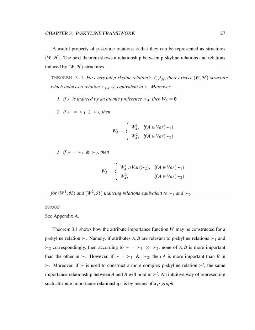
THEOREM 3.1 For every full p-skyline relation∈FH , there exists a (W,H )-structure
which induces a relation (W,H ) equivalent to . Moreover,
1. if is induced by an atomic preference >A, then WA = /0
2. if = 1 ⊗ 2, then
WA =
W 1A , if A ∈Var(1)
W 2A , if A ∈Var(2)
3. if = 1 & 2, then
WA =
W 1A ∪Var(2), if A ∈Var(1)
W 2A , if A ∈Var(2)
for (W 1,H ) and (W 2,H ) inducing relations equivalent to 1 and 2.
PROOF
See Appendix A.
Theorem 3.1 shows how the attribute importance function W may be constructed for a
p-skyline relation . Namely, if attributes A,B are relevant to p-skyline relations 1 and
2 correspondingly, then according to = 1 ⊗ 2, none of A,B is more important
than the other in . However, if = 1 & 2, then A is more important than B in
. Moreover, if is used to construct a more complex p-skyline relation ′, the same
importance relationship between A and B will hold in ′. An intuitive way of representing
such attribute importance relationships is by means of a p-graph.

CHAPTER 3. P-SKYLINE FRAMEWORK 28
DEFINITION 3.8 Let be a full p-skyline relation (i.e., a member of FH ) and (W,H )
be a structure which induces a relation equivalent to . A graph Γ whose nodes N(Γ)
are Var(), and whose edges are defined as
Γ = (X ,Y ) | X ,Y ∈Var()∧Y ∈WX
is the p-graph of .
According to Definition 3.8, the set of nodes of a p-graph is equal to the set of the
attributes relevant to the p-skyline relation. Edges in a p-graph go from more important
to less important attributes. By Theorem 3.1, a p-graph of a p-skyline relation can be
constructed recursively using the next corollary.
COROLLARY 3.1 Let be a full p-skyline relation. Then the edge set of the p-graph Γ
of is
1. empty, if is induced by an atomic preference;
2. Γ1 ∪ Γ2 , if = 1 ⊗ 2;
3. Γ1 ∪ Γ2 ∪ N(Γ1)×N(Γ2), if = 1 & 2;
We illustrate Corollary 3.1 in the next example.
EXAMPLE 3.3 Let A = A,B,C, H = >A,>B,>C, and
1 ≡ (A ⊗ B) & C
2 ≡ A ⊗ B ⊗ C
A relation equivalent to 1 is induced by the structure (W 1,H ) with W 1A = C,W 1
B =
C,W 1C = /0. The p-graph Γ1 of 1 is shown in Figure 3-2(a).

CHAPTER 3. P-SKYLINE FRAMEWORK 29
A B
C
(a) p-graph Γ1
A B C
(b) p-graph Γ2
Figure 3-2: p-graphs from Example 3.3
A relation equivalent to 2 is induced by the structure (W 2,H ) with W 2A = /0,W 2
B =
/0,W 2C = /0. The p-graph Γ2 of 2 is shown in Figure 3-2(b).
In the previous section, we showed that the skyline relation skyH is constructed as
Pareto accumulation of all the members of H . Hence, the next corollary holds.
COROLLARY 3.2 The p-graph ΓskyH of the skyline relation skyH is defined by the node
set N(ΓskyH ) = A and the edge set ΓskyH = /0.
The next theorem shows necessary and sufficient conditions for a directed graph to be
a p-graph of some p-skyline relation.
THEOREM 3.2 (SPO+Envelope)
A directed graph Γ with the node set A is a p-graph of a p-skyline relation iff
1. Γ is transitive and irreflexive, i.e. a strict partial order (SPO), and
2. Γ satisfies the Envelope property:
∀A,B,C,D ∈ A , all different
(A,B) ∈ Γ∧ (C,D) ∈ Γ∧ (C,B) ∈ Γ⇒ (C,A) ∈ Γ∨ (A,D) ∈ Γ∨ (D,B) ∈ Γ
As we showed above, a p-graph represents the relationships of importance between
attributes induced by the corresponding p-skyline relation. Hence, the SPO properties of a
p-graph are quite intuitive – they capture the rationality of the importance relationship. The

CHAPTER 3. P-SKYLINE FRAMEWORK 30
B D
A C
Figure 3-3: The Envelope property
Envelope property of a p-graph is due to the fact that each atomic preference relation can
have only one occurrence in a p-skyline preference relation. According to that property, if
a graph Γ has the three edges shown bold in Figure 3-3, then the p-graph must have at least
one of the dashed edges. It is easy to check that an equivalent formulation of Envelope
is that if Γ has the tree bold edges in Figure 3-3, then Γ must have at least one more edge
between the nodes A,B,C, and D that does not violate the SPO properties of Γ.
To prove Theorem 3.2, we introduce the notion of the typed partition of a directed
graph.
DEFINITION 3.9 Let Γ be a directed graph, and Γ1, Γ2 be two nonempty subgraphs of
Γ such that N(Γ1)∩N(Γ2) = /0 and N(Γ1)∪N(Γ2) = N(Γ). Then the pair of Γ1,Γ2 is a
∼-partition (→-partition) of Γ if Γ |= N(Γ1)∼ N(Γ2) ((N(Γ1),N(Γ2)) ∈ Γ, respectively).
The proof of Theorem 3.2 is based on lemmas 3.1 and 3.2. Lemma 3.1 establishes
relationships between nodes in an SPO+Envelope graph, while Lemma 3.2 establishes
relationships between typed partitions in such a graph.
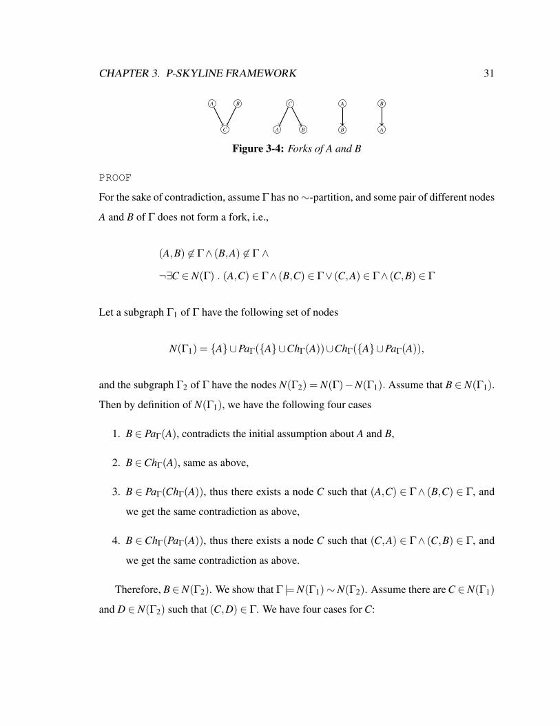
DEFINITION 3.10 Two nodes A and B of a directed graph Γ form a fork if A is differ-
ent from B, and there is a node C in Γ s.t.
(A,C) ∈ Γ∧(B,C) ∈ Γ∨ (C,A) ∈ Γ∧ (C,B) ∈ Γ, or
(A,B) ∈ Γ∨ (B,A) ∈ Γ
Figure 3-4 shows all possible forks of two nodes A and B in a graph.
LEMMA 3.1 Let a directed graph Γ satisfy SPO+Envelope. Then Γ has a ∼-partition,
or any pair of nodes of Γ form a fork.
CHAPTER 3. P-SKYLINE FRAMEWORK 31
A B
C A B
C A
B A
B
Figure 3-4: Forks of A and B
PROOF
For the sake of contradiction, assume Γ has no∼-partition, and some pair of different nodes
A and B of Γ does not form a fork, i.e.,
(A,B) 6∈ Γ∧ (B,A) 6∈ Γ ∧
¬∃C ∈ N(Γ) . (A,C) ∈ Γ∧ (B,C) ∈ Γ∨ (C,A) ∈ Γ∧ (C,B) ∈ Γ
Let a subgraph Γ1 of Γ have the following set of nodes
N(Γ1) = A∪PaΓ(A∪ChΓ(A))∪ChΓ(A∪PaΓ(A)),
and the subgraph Γ2 of Γ have the nodes N(Γ2) = N(Γ)−N(Γ1). Assume that B ∈ N(Γ1).
Then by definition of N(Γ1), we have the following four cases
1. B ∈ PaΓ(A), contradicts the initial assumption about A and B,
2. B ∈ChΓ(A), same as above,
3. B ∈ PaΓ(ChΓ(A)), thus there exists a node C such that (A,C) ∈ Γ∧ (B,C) ∈ Γ, and
we get the same contradiction as above,
4. B ∈ChΓ(PaΓ(A)), thus there exists a node C such that (C,A) ∈ Γ∧ (C,B) ∈ Γ, and
we get the same contradiction as above.
Therefore, B∈N(Γ2). We show that Γ |= N(Γ1)∼N(Γ2). Assume there are C ∈N(Γ1)
and D ∈ N(Γ2) such that (C,D) ∈ Γ. We have four cases for C:

CHAPTER 3. P-SKYLINE FRAMEWORK 32
1. C ∈ PaΓ(ChΓ(A)), i.e., there exists F such that (A,F) ∈ Γ ∧ (C,F) ∈ Γ. Given
(C,D) ∈ Γ, the Envelope property of Γ implies that
(C,A) ∈ Γ∨ (A,D) ∈ Γ∨ (D,F) ∈ Γ
Then the first disjunct implies that D ∈ ChΓ(PaΓ(A)), i.e., D ∈ N(Γ1); the second
disjunct implies that D ∈ ChΓ(A), i.e., D ∈ N(Γ1); the third disjunct implies that
D ∈ PaΓ(ChΓ(A)), i.e., D ∈ N(Γ1). This contradicts the assumption that D ∈ N(Γ2).
2. C ∈ ChΓ(PaΓ(A)), i.e., there exists F such that (F,A) ∈ Γ∧ (F,C) ∈ Γ. Then the
transitivity of Γ implies (F,D) ∈ Γ, i.e., D ∈ChΓ(PaΓ(A)) and thus D ∈ N(Γ1). Con-
tradiction.
3. C ∈ChΓ(A), and by transitivity of Γ, we get that D ∈ChΓ(A) and thus D ∈ N(Γ1).
Contradiction.
4. C ∈ PaΓ(A), thus D ∈ChΓ(PaΓ(A)) and D ∈ N(Γ1). Contradiction.
It can be shown that (D,C)∈ Γ leads to similar contradictions. Therefore, Γ |= N(Γ1)∼
N(Γ2). However, this contradicts the initial assumption.
LEMMA 3.2 A directed graph Γ satisfying SPO+Envelope with more than one node
has a→-partition or a ∼-partition into subgraphs Γ1,Γ2 satisfying SPO+Envelope.
PROOF
We assume that no ∼-partition of Γ exists and show that there exists a→-partition. Since
Γ is a finite SPO, there exists a nonempty set Top ⊆ N(Γ) of all the nodes which have no
incoming edges. If Top is a singleton, then clearly Top dominates every node in N(Γ)−
Top and we get a→-partition. Assume Top is not singleton. Pick any two nodes T1,T2 ∈
Top. Since T1 and T2 have no incoming edges, Lemma 3.1 implies that there exists a node
Z1 such that (T1,Z1) ∈ Γ∧ (T2,Z1) ∈ Γ. Pick some node Tk (Tk 6= T1,Tk 6= T2) from Top.
CHAPTER 3. P-SKYLINE FRAMEWORK 33
Since Tk has no incoming edges either, Lemma 3.1 implies that either Tk is a parent of
Z1 or they have a common child (which is also a child of T1 and T2 by transitivity of Γ).
Therefore, by picking every node of Top, we can show that there exists at least one node Z
which is a child of all nodes in Top. Let us denote as M the set of all the nodes such that
every node in Top dominates every node in M. Above we showed that M contains at least
one node.
Now let us show that if a node X is not in M then (X ,M) ∈ Γ. Clearly, if X ∈ Top,
then (X ,M) ∈ Γ. So let X 6∈ Top. By definition of Top, there is a node T1 ∈ Top such
that (T1,X) ∈ Γ. Assume there is a node Z ∈M such that (X ,Z) 6∈ Γ. By definition of M,
(T1,Z) ∈ Γ. Now pick some node T (T 6= T1) of Top. By definition of M, (T,Z) ∈ Γ. Let
us apply Envelope:
(T,Z) ∈ Γ ∧ (T1,Z) ∈ Γ ∧ (T1,X) ∈ Γ⇒ (T1,T ) ∈ Γ ∨ (T,X) ∈ Γ ∨ (X ,Z) ∈ Γ
The first and the last disjuncts in the right-hand-side of the expression contradict the as-
sumptions that T ∈ Top and (X ,Z) 6∈ Γ. Therefore, the only choice is (T,X)∈ Γ. However,
T is an arbitrary node in Top. Therefore, (Top,X) ∈ Γ and thus X ∈M by definition of M.
So if we construct a graph Γ1 with the node set N(Γ)−M, and Γ2 with the node set M,
they will be nonempty and thus a→-partition of Γ
It is easy to check that any subgraph of an SPO+Envelope graph satisfies that prop-
erty.
Now we return to the proof of Theorem 3.2.
PROOF OF THEOREM 3.2
By induction in the size of p-skyline relation, it is easy to show that p-graphs satisfy
SPO+Envelope. Now we show that any directed graph satisfying SPO+Envelope is
a p-graph of some p-skyline relation. Given such a graph, we construct the corresponding
CHAPTER 3. P-SKYLINE FRAMEWORK 34
p-skyline relation recursively. If Γ contains a single node, then the corresponding p-skyline
relation is induced by the atomic preference relation of the corresponding attribute-node. If
Γ has more than one node, then Γ has either a→-partition or a ∼-partition Γ1, Γ2 into non-
empty SPO+Envelope subgraphs (Lemma 3.2). Pick any such a partition Γ1, Γ2. If it is a
→-partition (∼-partition), then the corresponding p-skyline relation is a prioritized (Pareto,
respectively) accumulation of the p-skyline relations corresponding to Γ1 and Γ2. This
recursive construction exactly corresponds to the construction of the function W shown in
Theorem 3.1.
3.5 Properties of p-skyline relations
In this section, we show some properties of p-skyline relations. These properties are used
to efficiently perform some essential operations with p-skyline relations: checking equiv-
alence and containment of two p-skyline relations and testing dominance of a tuple over
another according to a p-skyline relation. Before going further, we note that since p-skyline
relations are representable as formulas (Proposition 3.3), one can use the corresponding
formulas to perform those operations. In this section, we show methods of performing the
operations above which do not use preference formulas.
We note that so far we have introduced two graph notations for p-skyline relations: p-
skyline syntax trees and p-graphs. Although these notations represent different concepts,
there is a correspondence between them shown in the next proposition.
PROPOSITION 3.4 (Syntax tree and p-graph correspondence) Let A and B be leaf
nodes in a syntax tree T of ∈ FH . Then (A,B) ∈ ΓΓ if and only if the least common
ancestor C of A and B in T is of type & , and A precedes B in left-to-right tree traversal.PROOF
⇐ Let C be a p-skyline relation represented by the syntax tree with the root node C.
Corollary 3.1 implies (A,B) ∈ ΓC . Corollary 3.1 also implies that ΓC ⊆ Γ.

CHAPTER 3. P-SKYLINE FRAMEWORK 35
⇒ Let (A,B) ∈ Γ. If C is of type & but B precedes A in left-to-right tree traversal, then
Corollary 3.1 implies (B,A) ∈ ΓC and hence (B,A) ∈ Γ, which is a contradiction to SPO
of Γ. If C is of type ⊗ , then by Corollary 3.1, ΓC |= A ∼ B and hence Γ |= A ∼ B,
which contradicts the initial assumption.
An important observation is that the proposition above as well as Corollary 3.1 describe
relationships between an accumulation-operator expression for a p-skyline relation and the
corresponding p-graph. However, the same p-skyline relation may be represented by two or
more different expressions of this type. An important question here is whether the p-graphs
which correspond to these expressions are equivalent. In the next theorem we show that
they really are.
THEOREM 3.3 (p-graph uniqueness) Two full p-skyline relations (i.e., members of
FH ) are equal if and only if their p-graphs are equal.
To prove the theorem, we use the next lemma.
LEMMA 3.3 Let for two full p-skyline relations 1,2∈ FH , (W 1,H ) and (W 2,H ) be
two structures inducing relations equal to 1 and 2, respectively. Let for some A ∈ A ,
W 1A −W 2
A 6= /0. Then there is a pair o,o′ ∈U such that
o1 o′,o 62 o′.
PROOF See Appendix A.
PROOF OF THEOREM 3.3.
⇒ Any two full p-skyline relations which have the same p-graph are represented by the
same structure (W,H ), by definition of p-graph. Therefore, the p-skyline relations are
equivalent.
⇐ Pick any equivalent full p-skyline relations 1 and 2. Let the structures (W 1,H ),
(W 2,H ) and the p-graphs Γ1 , Γ2 represent 1 and 2, respectively. Clearly, the node

CHAPTER 3. P-SKYLINE FRAMEWORK 36
sets of Γ1 and Γ2 are equal to A . If their edge sets are different, then the functions W 1
and W 2 are different. Pick any A ∈ A be such that W 1A 6= W 2
A . Without loss of generality,
we can assume W 1A −W 2
A 6= /0. Lemma 3.3 implies that 1 and 2 are not equivalent which
is a contradiction.
According to Theorem 3.3, to check equivalence of p-skyline relations, one only needs
to compare their p-graphs. As the next theorem shows, containment of p-skyline relations
may be also checked using their p-graph representations.
THEOREM 3.4 (p-skyline relation containment) For two full p-skyline relations
1,2 ∈ FH ,
1 ⊂ 2 ⇔ Γ1 ⊂ Γ2.
PROOF
⇐ Let (W 1,H ) and (W 2,H ) be the structures which induce relations the (W 1,H ) and
(W 2,H ) equivalent to 1 and 2 correspondingly. Γ1 ⊂ Γ2 implies that for all A ∈ A ,
W 1A ⊆W 2
A . Thus, (W 1,H ) ⊆ (W 2,H ) and 1 ⊆ 2. Theorem 3.3 implies 1 ⊂ 2.
⇒ Let Γ1 6⊂ Γ2 . If Γ1 = Γ2 , then by Theorem 3.3,1 =2 which is a contradiction.
Therefore, Γ1 6= Γ2 , and for some A we have W 2A −W 1
A 6= /0. Lemma 3.3 implies1 6⊂ 2
which is a contradiction.
Theorem 3.4 implies an important result. Recall that in Corollary 3.2 we showed that
the edge set of the p-graph ΓskyH of the skyline preference relation skyH is empty. Hence,
the following facts are implied by Theorem 3.4.
COROLLARY 3.3 The skyline relation skyH is the least full p-skyline relation in FH .
COROLLARY 3.4 For any relation instance r and any full p-skyline relations
1, 2 ∈ FH , such that 2 ⊂ 1, we have w1(r)⊆ w2(r)⊆ wskyH (r)

CHAPTER 3. P-SKYLINE FRAMEWORK 37
A1 A2 A3
(a) ΓskyH
A1 A2
A3
(b) Γ1
A2 A3
A1
(c) Γ2
A1 A2 A3t1 2 1 0t2 1 2 0t3 1 0 2t4 1 0 0
(d) r
Figure 3-5: Containment of p-skyline relations
The importance of Corollary 3.4 is that if we take any full p-skyline relation ∈ FH ,
the corresponding preference query result will always be contained in the corresponding
skyline. In real life, that means that if user preferences are modeled as p-skyline relations
instead of skyline relation, the sizes of the corresponding preference query results may be
smaller.
EXAMPLE 3.4 Let A = A1,A2,A3, and for every attribute, we prefer larger values.
Consider the relations skyH ,1,2
skyH = A1 ⊗ A2 ⊗ A3
1 = (A1 & A3) ⊗ A2
2 = (A2 & A1) ⊗ A3
whose p-graphs are shown in Figures 3-5(a), 3-5(b), and 3-5(c), correspondingly. The-
orems 3.4 and 3.3 imply that skyH ⊂ 1, skyH ⊂ 2, 1 6⊆ 2, and 2 6⊆ 1. Take
the relation r shown in Figure 3-5(d). Then wskyH (r) = t1, t2, t3, w1(r) = t1, t2, and
w2(r) = t2, t3.
In the next theorem, we show how one can test dominance of a tuple over another
according to a p-skyline relation without using the a preference formula.

CHAPTER 3. P-SKYLINE FRAMEWORK 38
THEOREM 3.5 (p-skyline dominance testing) Let be a full p-skyline relation, and
o,o′ ∈U such that o 6= o′. Let also BetterIn(o1,o2) = A | o1.A >A o2.A, Di f f (o1,o2)
be the set of attributes in which o1 and o2 are different, and Top(o1,o2) be the set of the
topmost elements of Di f f (o1,o2) in Γ. Then the following statements are equivalent:
1. o o′;
2. BetterIn(o,o′)⊇ Top(o,o′);
3. ChΓ(BetterIn(o,o′))⊇ BetterIn(o′,o).
The intuition beyond the theorem above is a follows. Method 2 of testing dominance
implies that o is preferred to o′ if and only if o is preferred to o′ according to all the most
important attributes in which these tuples are different. Method 3 of testing dominance
says that o is preferred to o′ if and only if for every attribute in which o′ is better than o,
there is a more important attribute in which o is better than o′.
PROOF
Let the structure (W,H ) induce a relation equivalent to , i.e.
= (W,H ) = TC
(⋃A∈A
pA
)
where
pA ≡ (o1,o2) | o1Ao2 ∩ ≈A−WA−A .
1⇔ 3 Let ChΓ(BetterIn(o,o′)) ⊇ BetterIn(o′,o). It is easy to check that the sequence
(Σo,o′,Ψo,o′) constructed as follows is a derivation sequence for o (W,H ) o′. Let Ψo,o′
be a sequence of all attributes in BetterIn(o,o′). For every Ai ∈ Ψo,o′ , let oi.Ai,oi+1.Ai
be equal to the values of Ai in o and o′ correspondingly. Let the values of the attributes
CHAPTER 3. P-SKYLINE FRAMEWORK 39
A1
A2
A3
A4
A5
A6
A7
(a) Γ
id A1 A2 A3 A4 A5 A6 A7t1 1 1 1 1 1 1 1t2 2 0 1 0 2 1 0t2 2 0 1 0 1 2 0
(b) Tuples to compare
Figure 3-6: Theorem 3.5 for dominance testing
BetterIn(o′,o)∩WAi be equal to those of o in oi and those of o′ in oi+1. Let the values of
the other attributes in oi,oi+1 be equal.
Now assume ChΓ(BetterIn(o,o′)) 6⊇ BetterIn(o′,o). Thus, the set BetterIn(o′,o)−
ChΓ(BetterIn(o,o′)) is nonempty. Similarly to the proof of Lemma 3.3, it can be shown
that no derivation sequence exists for o(W,H ) o′.
2⇔ 3 2 implies 3 by definition of Top(o,o′). Prove that 3 implies 2. Assume that 3 holds
but ∃A ∈ Top(o,o′)−BetterIn(o,o′). Since >A is a total order, A ∈ BetterIn(o′,o). Then
3 implies that A 6∈ Top(o,o′), which is a contradiction.
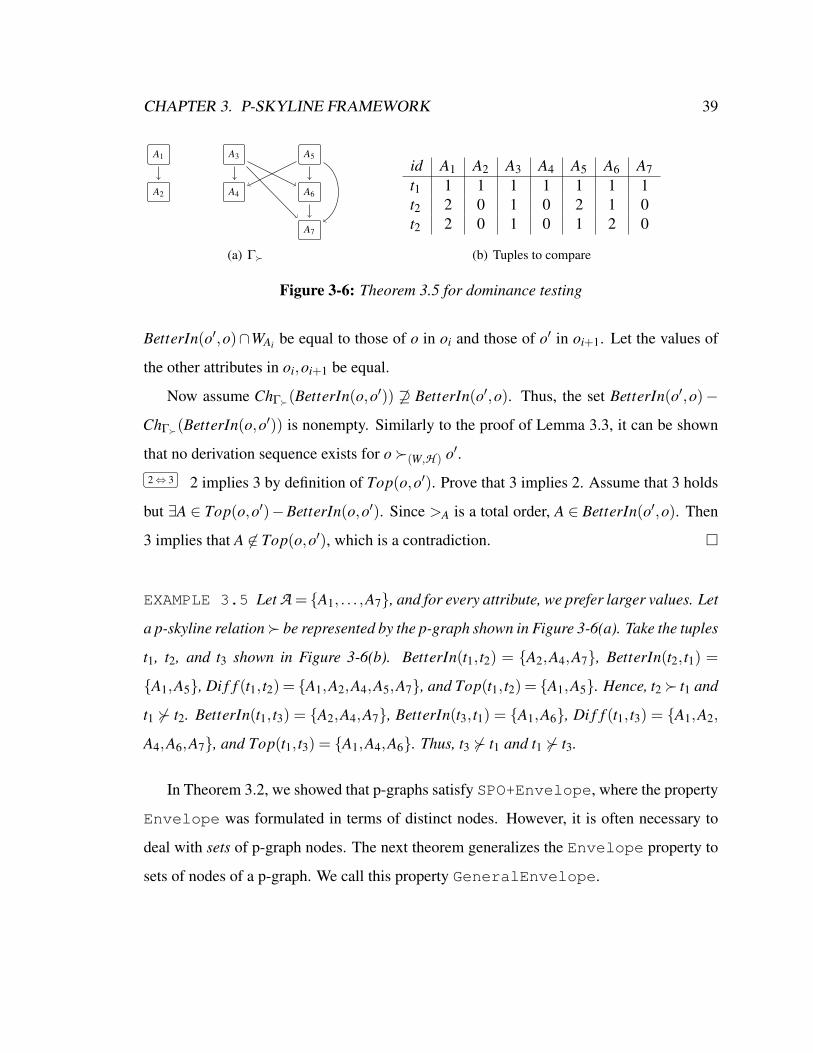
EXAMPLE 3.5 Let A = A1, . . . ,A7, and for every attribute, we prefer larger values. Let
a p-skyline relation be represented by the p-graph shown in Figure 3-6(a). Take the tuples
t1, t2, and t3 shown in Figure 3-6(b). BetterIn(t1, t2) = A2,A4,A7, BetterIn(t2, t1) =
A1,A5, Di f f (t1, t2) = A1,A2,A4,A5,A7, and Top(t1, t2) = A1,A5. Hence, t2 t1 and
t1 6 t2. BetterIn(t1, t3) = A2,A4,A7, BetterIn(t3, t1) = A1,A6, Di f f (t1, t3) = A1,A2,
A4,A6,A7, and Top(t1, t3) = A1,A4,A6. Thus, t3 6 t1 and t1 6 t3.
In Theorem 3.2, we showed that p-graphs satisfy SPO+Envelope, where the property
Envelope was formulated in terms of distinct nodes. However, it is often necessary to
deal with sets of p-graph nodes. The next theorem generalizes the Envelope property to
sets of nodes of a p-graph. We call this property GeneralEnvelope.

CHAPTER 3. P-SKYLINE FRAMEWORK 40
A1
A7
A2
A4
A3
A5 A6
Figure 3-7: The GeneralEnvelope property
THEOREM 3.6 (GeneralEnvelope) Let be a p-skyline relation with the p-graph
Γ. Let also A,B,C,D be disjoint node sets of Γ. Let the subgraphs of Γ induced by
those node sets be singletons or unions of at least two disjoint subgraphs. Then
(A,B) ∈ Γ ∧(C,D) ∈ Γ∧ (C,B) ∈ Γ⇒
(C,A) ∈ Γ∨ (A,D) ∈ Γ∨ (D,B) ∈ Γ
PROOF See Appendix A.
Unlike Envelope which holds for any combination of four different nodes, the prop-
erty of GeneralEnvelope holds for a certain class of disjoint node subsets. However,
that class is quite general. For instance, Var() induces disjoint subgraphs if is defined
as Pareto accumulation of p-skyline relations.
EXAMPLE 3.6 Let A = A1, . . . ,A7. Consider the p-graph Γ (Figure 3-7) of
= ((>A1 ⊗ >A2 ⊗ >A3) & (>A4 ⊗ >A5 ⊗ >A6)) ⊗ >A7
Take A = A1, B = A4, C = A2,A3, D = A5,A6. Then we have
(A,B) ∈ Γ∧ (C,D) ∈ Γ∧ (C,B) ∈ Γ∧ (A,D) ∈ Γ

CHAPTER 3. P-SKYLINE FRAMEWORK 41
3.6 Minimal extensions of p-skyline relations
Consider the following scenario. Let us have a full p-skyline relation (i.e., a member
of FH ) and two tuples o1 and o2 such that o1 6 o2. Assume that we have the following
problem: test if there is an extension ext ∈ FH of such that o1 6ext o2. In other words,
we need to check if is a maximal full p-skyline relation according to which o1 is not
preferred to o2. Problems of this type are considered in the next chapter where we show
an approach of discovering full p-skyline relation using user feedback. One approach to
solve this problem is to enumerate all extensions of in FH and test if o1 dominates o2
according to each of them. However, the number of such extensions may be quite large.
Instead, one could consider only minimal extensions of in FH : if according to some
minimal extension ext we have o1 6ext o2, then is not a maximal relation satisfying the
property, otherwise it is. In this section, we study the problem of computing efficiently all
full p-skyline relations which are minimal extensions of a given full p-skyline relation. The
formal definition of a minimal extension of a full p-skyline relation is given below.
DEFINITION 3.11 Given a full p-skyline relation ∈ FH , a full p-skyline relation
ext ∈ FH is a full p-skyline extension of if ⊂ ext . The extension ext is minimal if
there is no full p-skyline relation ′ ∈ FH such that ⊂ ′ ⊂ ext .
We showed in Theorem 3.4 that given any full p-skyline relation , a full p-skyline
extension ext of may be obtained by computing an extension Γext of the p-graph Γ.
Hence, the problem of computing a minimal full p-skyline extension of a p-skyline relation
can be reduced to the problem of finding a minimal set of edges that when added to Γ
form a graph satisfying SPO+Envelope. However, it is not clear how to find such a
minimal set of edges efficiently. Moreover, if one wants to compute all minimal full p-
skyline extensions of a p-skyline relation, then all minimal sets of such edges have to be
computed. Another problem of such an approach is that it may be the case that p-skyline
CHAPTER 3. P-SKYLINE FRAMEWORK 42
relations in a particular application are represented as accumulation operator expressions.
In this case, one needs to convert a p-skyline syntax tree to a p-graph, compute its minimal
SPO+Envelope extension, and then convert the p-graph back to a p-skyline syntax tree.
The method of computing all minimal extensions we propose here operates directly
with p-skyline relation expressions represented as p-skyline syntax trees. In particular,
we show a set of transformation rules of p-skyline syntax trees such that every unique
application of a rule from this set results in a unique minimal full p-skyline extension of the
original p-skyline relation. If all minimal full p-skyline extensions of a p-skyline relation
are needed, then one needs to apply to the syntax tree every rule in every possible way.
The transformation rules are shown in Figure 3-9. On the left hand side, we show a
part of the syntax tree of an original p-skyline relation. On the right hand side, we show
how the corresponding part is modified in the resulting relation. We assume that the rest of
the syntax tree is left unchanged. All the transformation rules perform some manipulations
with two children Ci and Ci+1 of a ⊗ -node of a syntax tree. For the sake of simplicity,
these nodes are shown as consecutive children. However, in the rules we assume that they
may be any pair of children nodes of the same ⊗ -node.
Let us denote the original relation as and the relation obtained as a result of applying
one of the transformation rules as ext . It can be easily checked by Corollary 3.1 that all
the rules only add edges to the p-graph of the original preference relation and hence extend
the p-skyline relation.
OBSERVATION 3.1 If T′ is obtained from T using any of Rule1, . . . ,Rule4, then Γ ⊂
Γ′ . Moreover,
• if T′ is a result of Rule1(T,Ci,Ci+1), then
Γ′−Γ = XY | X ∈Var(N1),Y ∈Var(Ci+1)

CHAPTER 3. P-SKYLINE FRAMEWORK 43
• if T′ is a result of Rule2(T,Ci,Ci+1), then
Γ′−Γ = XY | X ∈Var(Ci+1),Y ∈Var(Nm)
• if T′ is a result of Rule3(T,Ci,Ci+1), then
Γ′−Γ = (Ci,Ci+1)
• if T′ is a result of Rule4(T,Ci,Ci+1,s, t) for s ∈ [1,n−1], t ∈ [1,m−1], then
Γ′−Γ =XY | X ∈⋃
p∈1...s
Var(Np),Y ∈⋃
q∈t+1...n
Var(Mq) ∪
XY | X ∈⋃
p∈1...t
Var(Mp),Y ∈⋃
q∈s+1...m
Var(Nq)
We note that every & - and ⊗ -node in a p-skyline syntax tree has to have at least two
child nodes. This is because the operators & and ⊗ must have at least two arguments.
However, as a result of a transformation rule application, some & - and ⊗ -nodes may
have only one child node. These nodes are:
1. R′ if k = 2 for Rule1,Rule2,Rule3,Rule4;
2. R′2 if m = 2 for Rule1,Rule2;
3. R′3 or R′5 if s = 1 or s = m−1, respectively, for Rule4;
4. R′4 or R′6 if t = 1 or t = n−1, respectively, for Rule4.
In such cases, we remove the nodes with a single child and connect the child directly to
the parent, as shown in Figure 3-8.

CHAPTER 3. P-SKYLINE FRAMEWORK 44
Before singe-childnode elimination
δ
N
After singe-childnode elimination
N
Figure 3-8: Single-child node elimination (δ ∈ & , ⊗ )
THEOREM 3.7 (minimal full p-skyline extension) Let ∈ FH , and T be a nor-
malized syntax tree of . Then ext is a minimal full p-skyline extension of if and
only if the syntax tree Text of ext is obtained from T by a single application of a rule
from Rule1, . . . ,Rule4.
In order to prove Theorem 3.7 we introduce the notions of frontier nodes and top and
bottom components in syntax tree.
DEFINITION 3.12 The top (bottom) component of a p-skyline relation is
1. (, respectively), if is induced by an atomic preference relation;
2. 1 (m, respectively), if
= 1 & . . . & m
Note that the notions of top and bottom components are undefined for p-skyline rela-
tions defined as Pareto accumulation of p-skyline relations.
DEFINITION 3.13 Let T be a normalized syntax tree of a full p-skyline relation .
Let also C1 and C2 be two child nodes of a ⊗ -node C in T. Let ext be a full p-skyline
extension of , and the subgraphs of Γ and Γext induced by Var(C1) and Var(C2) be
equal. Let X ∈Var(C1), Y ∈Var(C2) be such that
(X ,Y ) ∈ Γext .
CHAPTER 3. P-SKYLINE FRAMEWORK 45
Then (C1,C2) is the frontier pair of T w.r.t. Text .
Given a frontier pair (C1,C2) of T w.r.t. Text , note that Γ |= Var(X) ∼ Var(Y ) by
Proposition 3.4. By definition, a p-skyline relation is constructed in a recursive way: a
higher level relation is defined in terms of lower level relations. Hence, the intuition beyond
the frontier pair is as follows. When and ext are constructed, the lower-level relations
C1 and C2 are present in both and ext . However, the next-level relations aggregating
C1 andC2 in andext are different since Γext has an edge from a member of Var(C1
) to a member of Var(C2) which is not present in Γ. The next lemma shows some
properties of frontier pairs.
LEMMA 3.4 Let ext be a full p-skyline extension of ∈ FH , and T be a normalized
syntax tree of . Let also (C1,C2) be a frontier pair of T w.r.t. Text . Denote the the top
and the bottom components of C1 as A1,B1, and the top and the bottom components of C2
as A2,B2. Then
(Var(A1),Var(B2)) ∈ Γext ∨ (Var(A2),Var(B1)) ∈ Γext
PROOF See Appendix A.
PROOF OF THEOREM 3.7
⇒ Let ext be a minimal extension of . We show here that there is ′∈ FH obtained
using a transformation rule Rule1, . . . ,Rule4 such that
⊂ ′ ⊆ ext . (3.3)
By the minimal extension property of ext that implies ′ = ext .
Theorem 3.4 implies that there are X ,Y such that (X ,Y ) ∈ Γext −Γ. Let (C1,C2) be a
frontier pair of T w.r.t. Text such that X ∈Var(C1) and Y ∈Var(C2). Lemma 3.4 implies
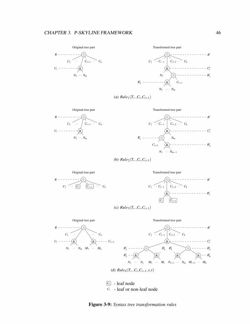
CHAPTER 3. P-SKYLINE FRAMEWORK 46
Original tree part
⊗
C1 . . .
&
Ci+1 . . . Ck
N1 . . . Nm
R
Ci
Transformed tree part
⊗
C1 . . . Ci−1 Ci+2 . . . Ck
&
N1 ⊗
Ci+1&
Nm. . .N2
R′
C′i
R′1
R′2
(a) Rule1(T,Ci,Ci+1)
Original tree part
⊗
C1 . . .
&
Ci+1 . . . Ck
N1 . . . Nm
R
Ci
Transformed tree part
⊗
C1 . . . Ci−1 Ci+2 . . . Ck
&
Nm⊗
Ci+1 &
Nm−1. . .N1
R′
C′i
R′1
R′2
(b) Rule2(T,Ci,Ci+1)
Original tree part
⊗
C1 . . . Ci Ci+1 . . . Ck
R
Transformed tree part
⊗
C1 . . . Ci−1 Ci+2 . . . Ck
&
Ci Ci+1
R′
R′1
(c) Rule3(T,Ci,Ci+1)
Original tree part
⊗
C1 . . . . . . Ck
&
N1 . . . Nm
&
M1 . . . Mn
R
Ci Ci+1
Transformed tree part
⊗
C1 Ci−1. . . Ci+2 . . . Ck
&
⊗
& &
Ns+1 . . . Nm Mt+1 . . . Mn
⊗
&&
Mt. . .M1Ns. . .N1
R′
C′i
R′2R′1
R′3
R′4 R′5
R′6
(d) Rule4(T,Ci,Ci+1,s, t)
Ci - leaf nodeCi - leaf or non-leaf node
Figure 3-9: Syntax tree transformation rules

CHAPTER 3. P-SKYLINE FRAMEWORK 47
that
(Var(A1),Var(B2)) ∈ Γext ∨ (Var(A2),Var(B1)) ∈ Γext (3.4)
for the top A1,A2 and the bottom B1,B2 components of C1 and C2 correspondingly. Con-
sider all possible types of C1 and C2. (i) Let C1,C2 be leaf nodes. Then ′ for which (3.3)
holds may be obtained by applying Rule3(T,C1,C2) (if the first disjunct of (3.4) holds) or
Rule3(T,C2,C1) (if the second disjunct of (3.4) holds). (ii) Let C1 be a & -node and C2 be
a leaf node. Then ′ may be obtained by applying Rule1(T,C1,C2) (if the first disjunct of
(3.4) holds) or Rule2(T,C1,C2) (if the second disjunct of (3.4) holds). Case (iii) when C1
is a leaf node and C2 is a & -node is similar to the previous case. Consider case (iv) when
C1 and C2 are & -nodes. Let the first disjunct of (3.4) hold. The case of the second disjunct
is analogous. We note that (Var(A1),Var(B1)) ∈ Γext and (Var(A2),Var(B2)) ∈ Γext .
This along with (3.4) is a condition for GeneralEnvelope:
(Var(A1),Var(A2)) ∈ Γext ∨ (Var(A2),Var(B1)) ∈ Γext ∨
(Var(B1),Var(B2)) ∈ Γext (3.5)
If the first disjunct of (3.5) holds, then′ can be obtained by applying Rule1(T,C1,C2). If
the last disjunct of (3.5) holds, then ′ can be obtained by applying Rule2(T,C2,C1). Let
the second disjunct of (3.5) hold, i.e. (Var(A2),Var(B1)) ∈ Γext . Let the child nodes of C1
and C2 be the sequences (A1 = N1, . . . ,Nm = B1) and (A2 = M1, . . . ,Mn = B2) correspond-
ingly. Since C1 and C2 are & -nodes, (Var(Ni),Var(N j)) ∈ Γ and (Var(Mi),Var(M j)) ∈
Γ for all i < j. Since ⊆ ext , the same edges are present in Γext . Note that (N1,Mn) ∈
Γext . Pick every child of C2 in its list of children from right to left and find the first index t
such that (Var(N1),Var(Mt)) 6∈ Γext but (Var(N1),Var(Mt+1)) ∈ Γext . If no such t exists,
then (Var(N1),Var(M1)) ∈ Γext and ′ may be obtained by applying Rule1(T,C1,C2).
So assume t ∈ [1,n]. Similarly, let s be the first index such that (Var(M1),Var(Ns)) 6∈ Γext

CHAPTER 3. P-SKYLINE FRAMEWORK 48
but (Var(M1),Var(Ns+1)) ∈ Γext . If s does not exist, then ′ may be obtained by ap-
plying Rule2(T,C2,C1). So assume s ∈ [1,m]. If both s and t are equal to 1, then ′
may be obtained using Rule4(T,C1,C2,s, t). In all other cases, it can be shown using
GeneralEnvelope that for all i ∈ [1,s], j ∈ [t +1,n] (Var(Ni),Var(M j)) ∈ Γext and for
all i ∈ [1, t], j ∈ [s+1,m] (Var(Mi),Var(N j)) ∈ Γext . Hence the Rule4(T,C1,C2,s, t) may
be used to construct ′ext .
⇐ We showed above that any minimal full p-skyline extension ext of may be com-
puted using a single application of one of the transformation rules. Showing that any valid
application of a transformation rule leads to a minimal full p-skyline extension of may
be done by using Lemma 3.4 and a case analysis similar to the one above.
Theorem 3.7 has two important corollaries describing properties of p-skyline relations.
COROLLARY 3.5 Given any full p-skyline relation with a normalized syntax tree T,
a syntax tree T′ of any its minimal full p-skyline extension ′ may be computed in time
O(|A |).
In Corollary 3.5, we assume the adjacency-list representation of syntax trees. The total
number of nodes in a tree is linear in the number of its leaf nodes [CLRS01] which are
A . Thus the number of edges in T is O(|A |). The transformation of T using any rule
requires removing O(|A |) and adding O(|A |) edges.
COROLLARY 3.6 For any full p-skyline relation , the number of its minimal full p-
skyline extensions is O(|A |4).
The justification for Corollary 3.6 is as follows. The set of minimal-extension rules is
complete due to Theorem 3.7. Every rule operates on two nodes Ci,Ci+1 of a syntax tree.
Hence, the number of such node pairs is O(|A |2). Rule4 also relies on some partitioning
of the sequence of child nodes of Ci and Ci+1. The total number of such partitionings is
O(|A |2). As a result, the total number of different rule applications is O(|A |4).
CHAPTER 3. P-SKYLINE FRAMEWORK 49
An important observation here is that the number of minimal full p-skyline extensions
is polynomial in the number of attributes. This differs from the number of all extensions of
a p-skyline relation. For instance, take the full p-skyline relation skyH . By Theorem 3.4,
any full p-skyline relation whose p-graph is a total order of A is a full p-skyline extension
of skyH . Theorem 3.3 implies that all p-skyline relations defined by different total-order
p-graphs are different. The number of such p-graphs is |A |!. Hence, the total number of
full p-skyline extensions of skyH is Ω(|A |!).
The last property of p-skyline relations which we state here and which is related to their
extensions is as follows. By Theorem 3.4, a full p-skyline extension of a p-skyline relation
is obtained by adding edges to its p-graph. However, the total number of edges in a
p-graph is at most O(|A |2). Hence, the next Corollary holds.
COROLLARY 3.7 Let S be a sequence of full p-skyline relations
1, . . . ,n ∈ FH
such that for all i ∈ [1,n− 1], we have that i+1 is a full p-skyline extension of i. Then
|S|= O(|A |2).
3.7 p-skyline query evaluation
Here we show some methods of winnow query evaluation for p-skyline relations. We
assume that we are given a full p-skyline relation , a database relation r instance, and
want to compute w(r), i.e. all the best tuples in r according to .
An important property of p-skyline relations is that they can be expressed using accu-
mulation operators. Hence, a winnow query with a p-skyline relation can be represented
as a Preference SQL query [KK02]. To do that, one needs to represent atomic preference
relations using certain base preference constructors. Moreover, by construction, the size

CHAPTER 3. P-SKYLINE FRAMEWORK 50
of a Preference SQL query based on p-skyline relation is linear in the number of attributes
involved in the preference relation. A number of optimization techniques have been devel-
oped for such queries [HK05].
Evaluating of p-skyline winnow queries as Preference SQL queries requires access to a
special query evaluation engine. If such an engine is not available, then general preference
query evaluation techniques may be used. Some query optimization techniques in this area
use preference-formula representation of a preference relation [Cho07a]. In Proposition
3.3, we showed that p-skyline relations can be represented as polynomial size preference
formulas.
A number of preference query evaluation methods developed for skyline queries can
also be applied to p-skyline winnow queries as well. One of them is BNL proposed in
[BKS01]. This algorithm relies on the efficiency of dominance testing for skyline relations.
As we showed here, dominance testing in the p-skyline framework can also be performed
efficiently: using Theorem 3.5 or preference formula evaluation.
Another skyline algorithm called SFS [CGGL03] may also be adopted to evaluate p-
skyline winnow queries. SFS uses the fact that for any SPO relation there exists a weak
order relation containing it. In that algorithm, tuples of a relation instance r are ordered
according to such a weak order, and then a version of BNL is run against the sorted r.
As we show here, a weak order relation containing a given full p-skyline relation can be
computed efficiently. By Theorem 3.4, a p-skyline relationext is a full p-skyline extension
of another p-skyline relation if the edge set of Γ is a subset of the edge set of Γext . By
Theorem 3.8, ext is a weak order if its p-graph is a total order of A . Moreover, since a
total order is a maximal SPO, for any p-graph there is a total order p-graph containing it.
Hence, the problem of computing a weak order p-skyline relationext containing can be
reduced to the problem of computing a total order graph containing Γ. That can be done
using topological sorting [CLRS01].
CHAPTER 3. P-SKYLINE FRAMEWORK 51
THEOREM 3.8 Let be a full p-skyline relation such that the p-graph Γ is a total
order of A . Then is a weak order.
PROOF
By Corollary 3.1, can be represented as
≡ (((A1 & A2) & A3) . . .) & An .
Let us denote A1 as 1, and i = i−1 & Ai . Then = n. We use induction to
show that n is a weak order. It is clear that a preference relation induced by an atomic
preference relation is a weak order since all atomic preference relations we consider here
are total orders. Hence, 1 is a weak order. Assume that i−1 is a weak order. Thus,
∀o1,o2,o3 . o1 i−1 o3⇒ o1 i−1 o2∨o2 i−1 o3. The relation i can be represented as
i = i−1 ∪ ≈Var(i−1) ∩ Ai .
We prove that ∀o1,o2,o3 . o1 i o3 ⇒ o1 i o2 ∨ o2 i o3, i.e., i is a weak order. Take
any o1,o2,o3 such that o1 i o3. If o1 i−1 o3, then o1 i−1 o2∨o2 i−1 o3 since i−1 is a
weak order. Hence, o1 i o2∨o2 i o3. Now let (o1,o3) ∈≈Var(i−1) ∩ Ai . If (o1,o2) or
(o2,o3) is in≈Var(i−1), then either (o1,o2) or (o2,o3) is in≈Var(i−1) ∩Ai becauseAi is
a total order. If neither (o1,o2) nor (o2,o3) is in ≈Var(i−1), then o1 i−1 o2 or o2 i−1 o3
by Theorem 3.5. Thus, o1 i o2∨o2 i o3, and i is a weak order.
3.8 Related work
The p-skyline framework is based on the preference constructor approach proposed by
Kießling in [Kie02]. That framework was extended in [Kie05] by relaxing definitions of

CHAPTER 3. P-SKYLINE FRAMEWORK 52
the accumulation operators and using SV-relations, instead of equality, as indifference re-
lations. [Kie05] shows that such an extension preserves the SPO properties of accumulated
relations. Moreover, the resulting accumulated relations were shown to be larger (in the
set theoretic sense) than the relations composed using the equality-based accumulational
operators. However, the problems of relative importance of attributes induced by such pref-
erence relations were not addressed in [Kie02] and [Kie05]. The problems of containment
of preference relations and minimal extensions were also not considered.
The original skyline framework was proposed by Borzsonyi et al in [BKS01], where
they proposed an extension of SQL in which the skyline operator can be intuitively repre-
sented. They also showed a number of algorithms for computing skylines: the block nested
loop algorithm (BNL) and divide-and-conquer algorithm with some optimizations. Since
then, a number of algorithms of computing skylines have been proposed. [TEO01] devel-
oped two algorithms – Bitmap and Index – to compute skyline points progressively. An-
other progressive skyline computation algorithm was proposed by Kossmann in [KRR02].
In the SFS algorithm proposed in [CGGL03], Chomicki et al showed that sorting a relation
before computing a skyline over it using BNL gives computational benefits. In [CET05],
Chan et al studied the problem of computing skylines with SPO atomic preferences. Some
algorithms for progressive computation and maintenance of skylines were proposed by Lee
in [LZLL07]. In [GSG07], Godfrey et al proposed the LESS skyline algorithm. It extends
SFS by performing early elimination of tuples which are guaranteed not to be skyline tu-
ples. To do that, [GSG07] proposed to use a window of tuples with high values of the
entropy score. It was shown there that tuples with higher values of this score tend to domi-
nate a large number of tuples. In that work, Godfrey et al performed a thorough analysis of
running time of some widely used skyline algorithms.
In [GSG05] Godfrey at al showed that the number of skyline points in a dataset may
be exponential in the number of attributes. Hence, if many attributes are relevant to user
CHAPTER 3. P-SKYLINE FRAMEWORK 53
preferences, then the set of the best tuples according to such a preference relation may be
rather large. A number of variants of the skyline operator have been proposed to solve the
large-skyline-size problem. Chan et al [CJT+06] propose to compute the set of k-dominant
skyline points instead of the entire skyline. A point p is said to k-dominate another point
q if there are k dimensions in which p is better than or equal to q, and in at least one
dimension, p is better than q. A point that is not k-dominated by other points is in the
k-dominant skyline. It was shown there that the existing skyline algorithms cannot be used
to compute k-dominant skylines. Chan et al proposed several algorithms for such compu-
tations. Another variant of the skyline operator was presented in [LYZZ07]. It computes
k most representative tuples of a skyline. k skyline points are called most representative
if the number of points which are dominated by them is maximized. It was shown there
that in the case of two attributes, the problem of computing the k most representative sky-
line tuples has an efficient polynomial solution. When the number of involved attributes is
greater than two, the problem is NP-hard in general. For such cases, [LYZZ07] proposed a
polynomial time approximation algorithm.
Another direction of research considered in the skyline framework is subspace skyline
[PJET05, YLL+05]. It is motivated by the fact that when a user provides a set of relevant
attributes and the corresponding atomic preferences, he or she may decide later that some
of them are not actually relevant and need not be considered. Hence there is a need in
computing skyline not only over a given set of atomic preferences but also over its subsets.
Such skylines are called subspace skylines. One interesting problem in this framework is
to identify the subspaces such that a given tuple belongs to the corresponding skylines. In
[PJET05], Pei et al showed an approach of computing such subspaces using the notion of
decisive subspace. Another problem here is related to the computation of subspace sky-
lines. It is clear that a subspace skyline may be computed using any skyline algorithm.
However, to compute k subspace skylines (for k different subsets of relevant atomic pref-
CHAPTER 3. P-SKYLINE FRAMEWORK 54
erences), such method may be inefficient since it does not use the information of possi-
ble similarity of the corresponding subspace skylines. To make the computation efficient,
[PJET05] proposed an algorithm for computing all subspaces skylines at once. Another
method computing all subspace skylines was proposed by Yuan et al in [YLL+05]. It is
based on the notion of skyline cube. It was shown there that if there are no two tuples in a
dataset which share a value of the same attribute (this property is called the distinct value
property), then the skyline of a smaller subspace is contained in the skyline of a larger sub-
space. Yuan et al [YLL+05] used that property to compute a skyline cube – the set of all
the subspace skylines for a given set of atomic preferences. The skyline cube approach was
used by Lee et al in [LwYwH09] to find the most interesting subspaces given the maximum
on the size of the corresponding skyline and a total order of attributes which represents the
importance of attributes for a user.
We note that the approach of subspace skyline is in a sense orthogonal to the p-skyline
framework proposed here. Both approaches extend the skyline framework. In the sub-
space skyline framework, the relative importance of attributes is fixed (i.e., all considered
attributes are of equal importance) while the sets of the corresponding attributes may vary.
In the p-skyline approach, the set of relevant attributes is fixed while the relative impor-
tance of them may vary. However, given a set of atomic preference relations, all subspace
skylines and the results of all full p-skyline relations are subsets of the (full-space) skyline
(under the distinct value property in the former case).

Chapter 4Discovery of p-skyline relations
In Chapter 3, we proposed a class of preference relations called p-skyline relations. In this
chapter, we introduce a method of constructing p-skyline relations based on user provided
feedback.
4.1 Feedback based discovery of p-skyline relations
As we showed in the previous chapter, the p-skyline framework is a generalization of the
skyline framework. The main difference between them is that in the p-skyline framework,
we can deal with variable attribute importance. However, one of the main properties of
the skyline framework is the simplicity of representing preferences. Namely, one needs to
provide only a set of atomic preferences to construct a preference relation. For p-skylines,
an additional piece of information – the relative importance of the attributes – has to be
provided by a user. However, requiring users to describe attribute importance explicitly
seems impractical for several reasons. First, the number of comparisons may be rather
large: one has to compare all attributes pairwise. The second issue is even more serious –
users themselves may be not fully aware of their own preferences.
In this chapter, we propose an alternative approach to discovering attribute importance
55
CHAPTER 4. DISCOVERY OF P-SKYLINE RELATIONS 56
relationships, based on user feedback. We use the following scenario of p-skyline relation
discovery. A fixed set of tuples describing real objects is stored in a database relation O ⊆
U. We assume that the user has preferences over these objects. Given O, she can partition
it into disjoint subsets: the set G of tuples she confidently likes (superior examples), the
set W of tuples she confidently dislikes (inferior examples), and the set of remaining tuples
about which she is not sure. We assume here that if a tuple o is inferior, then there is at least
one superior example which the user likes more than o. This assumption is justified by a
general principle that we consider something bad because we know of a better alternative.
Given that setup, we aim to compute a p-skyline relation according to which all tuples in G
are superior and all tuples in W are inferior.
Recall that any p-skyline relation is defined by the following parameters:
• the set of relevant attributes;
• atomic preferences over the relevant attributes; and
• the combination of accumulation operators which are used to combine the atomic
preferences into one relation.
Hence, the problem of discovery of a p-skyline relation based on user feedback can be
decomposed into three problems of discovering each of the parameters above. We note
that the first two problems have been studied in many frameworks of preference discov-
ery. Some methods of solving them are shown in Section 4.6. Here we focus on the last
problem: computing a p-skyline relation based on user feedback given that the set of rel-
evant attribute is the entire set of attributes A . In addition to that, we assume that atomic
preference relations H are also known.
Having subsets G and W of a set of tuples O, we want to find a possible p-skyline
relation which implies G being superior and W being inferior examples in O. Formally, we
want to compute a full p-skyline relation (i.e., a member of FH ) such that 1) G⊆w(O)
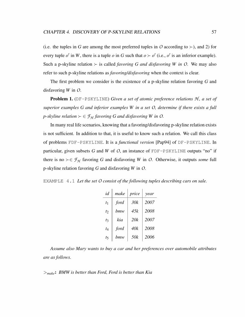
CHAPTER 4. DISCOVERY OF P-SKYLINE RELATIONS 57
(i.e. the tuples in G are among the most preferred tuples in O according to ), and 2) for
every tuple o′ in W , there is a tuple o in G such that o o′ (i.e., o′ is an inferior example).
Such a p-skyline relation is called favoring G and disfavoring W in O. We may also
refer to such p-skyline relations as favoring/disfavoring when the context is clear.
The first problem we consider is the existence of a p-skyline relation favoring G and
disfavoring W in O.
Problem 1. (DF-PSKYLINE) Given a set of atomic preference relations H , a set of
superior examples G and inferior examples W in a set O, determine if there exists a full
p-skyline relation ∈ FH favoring G and disfavoring W in O.
In many real life scenarios, knowing that a favoring/disfavoring p-skyline relation exists
is not sufficient. In addition to that, it is useful to know such a relation. We call this class
of problems FDF-PSKYLINE. It is a functional version [Pap94] of DF-PSKYLINE. In
particular, given subsets G and W of O, an instance of FDF-PSKYLINE outputs “no” if
there is no ∈ FH favoring G and disfavoring W in O. Otherwise, it outputs some full
p-skyline relation favoring G and disfavoring W in O.
EXAMPLE 4.1 Let the set O consist of the following tuples describing cars on sale.
id make price year
t1 ford 30k 2007
t2 bmw 45k 2008
t3 kia 20k 2007
t4 ford 40k 2008
t5 bmw 50k 2006
Assume also Mary wants to buy a car and her preferences over automobile attributes
are as follows.
>make: BMW is better than Ford, Ford is better than Kia

CHAPTER 4. DISCOVERY OF P-SKYLINE RELATIONS 58
>year: higher values of year (i.e., newer cars) are preferred
>price: lower values of price (i.e., cheaper cars) are preferred
Let G = t4, W = t3. We discover a full p-skyline relation favoring G and disfa-
voring W. First, >make cannot be more important than all other attribute preferences since
then t2 and t5 dominate t4 and thus t4 is not superior. Moreover, >price cannot be more im-
portant than the other attribute preferences because then t3 and t1 dominate t4. However,
if >year is more important than the other attribute preferences, then t4 dominates t3 and no
other tuple dominates t4 in >year. At the same time, both t2 and t4 are the best according
to >year, but t2 may dominate t4 in make. Therefore, >make should not be more important
than >price. Thus, the following p-skyline relation favors G and disfavors W in O
1 = year & (price ⊗ make)
The set of the best tuples in O according to 3 is t2, t4.
Generally there may be zero or more full p-skyline relations favoring G and disfavoring
W in O. When more than one such preference relation exists, we pick the largest ones
(in the set theoretic sense). Larger preference relations imply more dominated tuples and
fewer most preferred ones. Consequently, the result of w(O) gets more manageable due
to its decreasing size. Moreover, maximizing corresponds to minimizing w(O)−G,
which implies more precise correspondence of to the real user preferences. A maximal
full p-skyline relation favoring G and disfavoring W in O is called optimal.
Thus, the second problem considered here is computing an optimal p-skyline relation
favoring G and disfavoring W .
Problem 2. (OPTIMAL FDF-PSKYLINE) Given a set of atomic preference relations
H , a set of superior examples G and inferior examples W of a set O, compute an optimal
p-skyline relation ∈ FH favoring G and disfavoring W in O.
CHAPTER 4. DISCOVERY OF P-SKYLINE RELATIONS 59
EXAMPLE 4.2 Take G, W, and 1 from Example 4.1. Note that in order to make t4
dominate t2, we need to make price more important than year. As a result, the relation
2 = year & price & make
also favors G and disfavors W in O but the set of best tuples in O according to 2 is t4.
Moreover, 2 is optimal. The justification is that no other p-skyline relation favoring G
and disfavoring W contains 2 since the p-graph of 2 is a total order of the attributes
year, price,make and thus is a maximal SPO.
Even though the notion of optimal favoring/disfavoring reduces the space of alternative
p-skyline relations, there still may be more than one optimal favoring/disfavoring p-skyline
relation, given G, W , and O.
4.2 Constraints to discover p-skyline relations
In this section, we show constraints that apply to the p-graph of a p-skyline relation and
that guarantee that the corresponding p-skyline relation favors G and disfavors W in O.
Let us consider the notion of favoring G in O first. For any member o′ ∈ G to be in the
set of the most preferred tuples of O, o′ must not be dominated by any tuple in O. That is,
∀o ∈ O,o′ ∈ G . o 6 o′ (4.1)
Using Theorem 3.5, we can rewrite (4.1) as
∀o ∈ O,o′ ∈ G . ChΓ(BetterIn(o,o′)) 6⊇ BetterIn(o′,o), (4.2)
for BetterIn(o1,o2) = A | o1.A >A o2.A. Note that no tuple can be preferred to itself by

CHAPTER 4. DISCOVERY OF P-SKYLINE RELATIONS 60
irreflexivity of . Therefore, a p-skyline relation favoring G in O should satisfy (|O|−1) ·
|G| negative constraints τ in the form:
τ : ChΓ(Lτ) 6⊇ Rτ
where Lτ = BetterIn(o,o′),Rτ = BetterIn(o′,o). We denote this set of constraints as
N (G,O).
EXAMPLE 4.3 Take Example 4.1. Then any p-skyline relation∈FH favoring G = t3
in O has to satisfy each negative constraint below
t1 6 t3 ChΓ(make) 6⊇ price
t2 6 t3 ChΓ(make,year) 6⊇ price
t4 6 t3 ChΓ(make,year) 6⊇ price
t5 6 t3 ChΓ(make) 6⊇ price,year
Now consider the notion of disfavoring W in O. According to the definition, a p-skyline
relation disfavors W in O if and only if the following holds
∀o′ ∈W ∃o ∈ G . o o′. (4.3)
Following Theorem 3.5, it can be rewritten as a set of positive constraints P (W,G)
∀o′ ∈W∨
oi∈G
ChΓ(BetterIn(oi,o′))⊇ BetterIn(o′,oi). (4.4)
Therefore, in order for to disfavor W in O, its p-graph Γ has to satisfy |W | positive
constraints.
EXAMPLE 4.4 Take Example 4.1. Then any p-skyline relation ∈ FH favoring G =
CHAPTER 4. DISCOVERY OF P-SKYLINE RELATIONS 61
t1, t3 and disfavoring W = t4 in O has to satisfy the constraint
t1 t4∨ t3 t4
which is equivalent to the following positive constraint
ChΓ(price)⊇ year∨ChΓ(price)⊇ year,make
Let us summarize the constraints we have considered here. In order to construct a p-
skyline relation favoring G and disfavoring W in O, we need to construct an attribute
importance graph Γ which satisfies SPO+Envelope to guarantee that is a p-skyline
relation, N (G,O) to guarantee favoring G in O, and P (W,G) to guarantee disfavoring W
in O.
By Theorem 3.4, a p-graph of an optimal is maximal among all graphs which satisfy
SPO+Envelope, N (G,O), and P (W,G).
4.3 Using superior/inferior examples for p-skyline discov-
ery
In this section, we study the problems of existence of a favoring/disfavoring p-skyline re-
lation and computing a favoring/disfavoring p-skyline relation. We start with the problem
existence of such a relation.
THEOREM 4.1 DF-PSKYLINE is NP-complete.
PROOF
The favoring/disfavoring p-skyline existence problem is in NP since checking if a p-skyline
relation favors G and disfavors W in O can be done in polynomial time by evaluating

CHAPTER 4. DISCOVERY OF P-SKYLINE RELATIONS 62
w(O), checking G ⊆ w(O), and checking if for every member of W there is a member
of W dominating it.
In order to show the hardness result, we do a polynomial-time reduction from SAT.
This is a two-step reduction. First, we show that for every instance φ of SAT there are
corresponding instances of positive P and negative N constraints, and φ has a solution
iff P and N are satisfiable. Second, we show that for every such P and N there are
corresponding instances of G, W , and O.
Consider instances of SAT in the following form
φ(x1, . . . ,xn) = ψ1(x1, . . . ,xn)∧ . . .∧ψm(x1, . . . ,xn)
where
ψt(x1, . . . ,xn) = xit ∨ . . .∨ x jt
For every instance of φ, construct A = c,y1,y1,y′1, . . . ,yn,yn,y′n. The sets of positive
and negative constraints are constructed as follows. For every variable xi,
1. Create positive constraints
χi :(yi,c) ∈ Γ∨ (yi,c) ∈ Γ
πi :(yi,y′i) ∈ Γ
2. Create negative constraints
λ1i :(yi,yi) 6∈ Γ
λ2i :(yi,y′i) 6∈ Γ
λ3i :(y′i,c) 6∈ Γ

CHAPTER 4. DISCOVERY OF P-SKYLINE RELATIONS 63
Now, for every ψt(x1, . . . ,xn) = xit ∨ . . .∨ x jt of φ construct the following positive constraint
µt : (yit ,c) ∈ Γ∨ . . .∨ (yit ,c) ∈ Γ
where yi =
yi if xi = xi
yi if xi = xi
.
We claim that there is a satisfying assignment (vi, . . . ,vn) for φ iff there is a p-graph
satisfying all the constraints above. First, assume there is a p-graph Γ satisfying all the
constraints above. Construct the assignment v = (vi, . . . ,vn) as follows:
vi =
0 if (yi,c) ∈ Γ
1 if (yi,c) ∈ Γ
.
Since Γ satisfies all χi, for every i we have (yi,c) ∈ Γ or (yi,c) ∈ Γ. Thus, every vi
will be assigned to some value according to the rule above. Now prove that vi is assigned
to only one value, i.e., we cannot have both (yi,c) ∈ Γ and (yi,c) ∈ Γ. Since Γ satisfies πi,
we have (yi,y′i) ∈ Γ. Thus having both (yi,c) ∈ Γ and (yi,c) ∈ Γ and Envelope implies
(yi,yi) ∈ Γ∨ (yi,y′i) ∈ Γ∨ (y′i,c) ∈ Γ
However, the expression above violates the constraints λ1i ,λ
2i ,λ
3i . Therefore, exactly one of
(yi,c) ∈ Γ, (yi,c) ∈ Γ holds.
Take every µt . Since it is satisfied by Γ, the corresponding ψi must be also satisfied by
construction of µt . Therefore, φ is also satisfied.
Now assume that there is an assignment (v1, . . . ,vn) satisfying φ. Show that there is a
p-graph Γ satisfying all the constraints above. Here we construct such a graph.

CHAPTER 4. DISCOVERY OF P-SKYLINE RELATIONS 64
For every i ∈ [1,n], draw the edge
(yi,c) ∈ Γ if vi = 1, and (P1)
(yi,c) ∈ Γ, otherwise (P2)
This satisfies the constraint χi. Moreover, all the constraints µt are satisfied by construction.
Now, for every i ∈ [1,n], draw the edge
(yi,y′i) ∈ Γ (P3)
which satisfies the constraint πi. As a result, all positive constraints are satisfied. Moreover,
none of the edges above violates any negative constraint. Thus, all the constraints above
are satisfied.
In additional the edges above, let us draw the following edges
1. for every i, j such that vi = 0,v j = 0, draw the edge
(yi,y′j) ∈ Γ (P4)
It is clear that these edges do not violate any negative constraints above.
2. for every i, j such that vi = 0,v j = 1, draw the edge
(yi,y j) ∈ Γ (P5)
Since i 6= j, this edge does not violate any negative constraints above.
It is easy to verify that the constructed graph Γ satisfies SPO+Envelope and all the
negative and positive constraints above.

CHAPTER 4. DISCOVERY OF P-SKYLINE RELATIONS 65
Now let us show that there exist sets of objects O, G and W which can be used to obtain
the constraints χi,πi,λ1i ,λ
2i ,λ
3i ,µt . Let for every attribute in A , its domain contain at least
three numbers −1,0,1, and greater values of be preferred. Here we construct the sets G,
W , M, and O = G∪W ∪M that generate the positive and negative constraints above.
1. Let G consist of a single object g with all attributes values are 0.
2. Let W = b1, . . . ,bn,u1, . . . ,un,w1, . . . ,wm be constructed as follows:
• for every i ∈ [1, . . . ,n], let all the attributes of bi be equal to 0 except for the
value of yi be −1 and y′i be 1.
• for every i ∈ [1, . . . ,n], let all the attributes of ui be equal to 0 except for the
values of yi,yi be equal to −1 and the value of c be equal to 1.
• take every t ∈ [1, . . . ,m] and let µt : (yit ,c) ∈ Γ∨ . . .∨ (y jt ,c) ∈ Γ, where yi ∈
yi,yi. Let all attributes of wt be equal to 0 except for the value of c be 1, and
the values of yit , . . . , y jt (whatever they are) be −1.
3. Let M = m11,m
21,m
31, . . . ,m
1n,m
2n,m
3n be constructed as follows. For all i ∈ [1, . . . ,n],
• Let all attributes of m1i be 0 except for yi and yi be −1 and 1 respectively.
• Let all attributes of m2i be 0 except for yi and y′ibe 1 and −1 respectively.
• Let all attributes of m3i are 0 except for y′i and c be 1 and −1 respectively.
It can be easily shown that these sets of objects induce the set of constructed constraints.
Now consider the problems of computing favoring/disfavoring p-skyline relations. First,
we consider the problem of computing any p-skyline relation favoring G and disfavoring
W in O, not necessary minimal. After that, we address the problem of computing optimal
p-skyline relations. The results shown below are based on the following lemma.

CHAPTER 4. DISCOVERY OF P-SKYLINE RELATIONS 66
LEMMA 4.1 Take a full p-skyline relation , and subsets G and W of O. Then the next
two operations can be done in polynomial time:
1. verifying if is optimal favoring G and disfavoring W in O;
2. computing an optimal p-skyline relation ext favoring G and disfavoring W in O
which is a full p-skyline extension of .
PROOF
See Appendix A.
THEOREM 4.2 FDF-PSKYLINE is FNP-complete
PROOF
Given two disjoint subsets G and W of O and∈FH , checking if favors G and disfavors
W in O can be done in polynomial time. In particular, one needs to compute w(O),
check G ⊆ w(O) and verify if for every o ∈W there is o′ ∈ G such that o′ o. Hence,
FDF-PSKYLINE is in FNP.
Now show that FDF-PSKYLINE is FNP-hard. To do that, we use a reduction from
FSAT. In particular, we find functions R and S, both computable in logarithmic space, such
that 1) for any instance x of FSAT, R(x) is an instance of FDF-PSKYLINE, and 2) for
any correct output z of R(x), S(z) is a correct output of x. For such a reduction, we use
the construction from the proof of Theorem 4.1. There we showed how a relation (denote
it as ) satisfying all the constraints (and thus favoring the constructed G and W ) may be
obtained. In the current reduction, if there is a p-skyline relation favoring G and disfavoring
W in O, then the relation itself is returned. Otherwise, “no” is returned.
The function R mentioned above has to convert an instance of FSAT to an instance of
FDF-PSKYLINE (i.e., G, W , and O). In the reduction shown in the proof of Theorem 4.1,
such a transformation is done via a set of constraints. However, it is easy to observe that

CHAPTER 4. DISCOVERY OF P-SKYLINE RELATIONS 67
such a construction can be performed using the corresponding instance of FSAT. By the
construction, the sets G, M, and the subset b1, . . . ,bn,u1, . . . ,un of W are common for
any instance of FSAT with n variables. To construct the subset w1, . . . ,wm of W , one can
use the expression ψt instead of the corresponding constraint µt . It is clear that the function
R performing such a transformation can be evaluated in logarithmic space.
We construct the function S as follows. If the instance of FDF-PSKYLINE returns
“no”, S returns “no”. Otherwise, it constructs the satisfying assignment (v1, . . . ,vn) in the
following way: for every i, vi is set to 1 if the p-graph contains the edge (yi,c) ∈ Γ, and 0
otherwise. It is clear that such a computation may be done in logarithmic space.
Surprisingly, the problem of computing an optimal favoring/disfavoring p-skyline rela-
tion is not harder then the problem of computing any favoring/disfavoring p-skyline rela-
tion.
THEOREM 4.3 OPTIMAL FDF-PSKYLINE is FNP-complete
PROOF
Given ∈ FH , checking if it is optimal favoring G and disfavoring W can be done in
polynomial time (Lemma 4.1). Hence, OPTIMAL FDF-PSKYLINE is in FNP.
To show that it is FNP-hard, we reduce from FDF-PSKYLINE. Here we construct
the function F that takes a p-skyline relation or “no” and returns a p-skyline relation or
“no”. F returns “no” if its input is “no”. If its input is a p-skyline relation , it returns
an optimal extension of as shown in Lemma 4.1. As a result, F returns an optimal
favoring/disfavoring p-skyline relation iff the corresponding favoring/disfavoring p-skyline
relation exists. The functions R and S transforming inputs of FDF-PSKYLINE to inputs
of OPTIMAL FDF-PSKYLINE and outputs of OPTIMAL FDF-PSKYLINE to outputs
of FDF-PSKYLINE correspondingly are trivial and hence are computable in logspace.
Therefore, FDF-PSKYLINE is FNP-complete.

CHAPTER 4. DISCOVERY OF P-SKYLINE RELATIONS 68
In view of Theorems 4.1, 4.2, and 4.3, we consider restricted versions of the favor-
ing/disfavoring p-skyline relation problems. We will assume that there are no inferior ex-
amples (W = /0).
4.4 Using only superior examples for p-skyline discovery
By definition of the problem of discovering favoring/disfavoring p-skyline relations, a user
is required to identify superior as well as inferior examples in a set of tuples. In many real
life scenarios, users are only indirectly involved in the process of identifying such classes.
For instance, the click-through rate may be used to measure the popularity of products.
Using this metric, it is easy to find the superior examples – the tuples with the highest
click-through rate. However, the problem of identifying inferior examples – those which
the user confidently dislikes – is harder. Namely, low click-through rate may mean that
a tuple is inferior, as well as that the user does not know about it, or it simply does not
satisfy the search criteria. Thus, there is a need for discovery of p-skyline relations based
on superior examples only.
Let us denote the subclasses of DF-PSKYLINE, FDF-PSKYLINE, and OPTIMAL
FDF-PSKYLINE in which the sets of inferior examples W are empty as F-PSKYLINE,
FF-PSKYLINE, and OPTIMAL FF-PSKYLINE, correspondingly.
As we show further, these problems are simpler than the corresponding problems for
favoring/disfavoring p-skyline relations. In particular, we show polynomial time algorithms
for all of them.
Consider F-PSKYLINE first. In Corollary 3.4 we showed that the set of the best objects
according to the skyline preference relation is the largest among all p-skyline relations.
Hence, the next proposition holds.
PROPOSITION 4.1 There exists a full p-skyline relation ∈FH favoring G in O if and
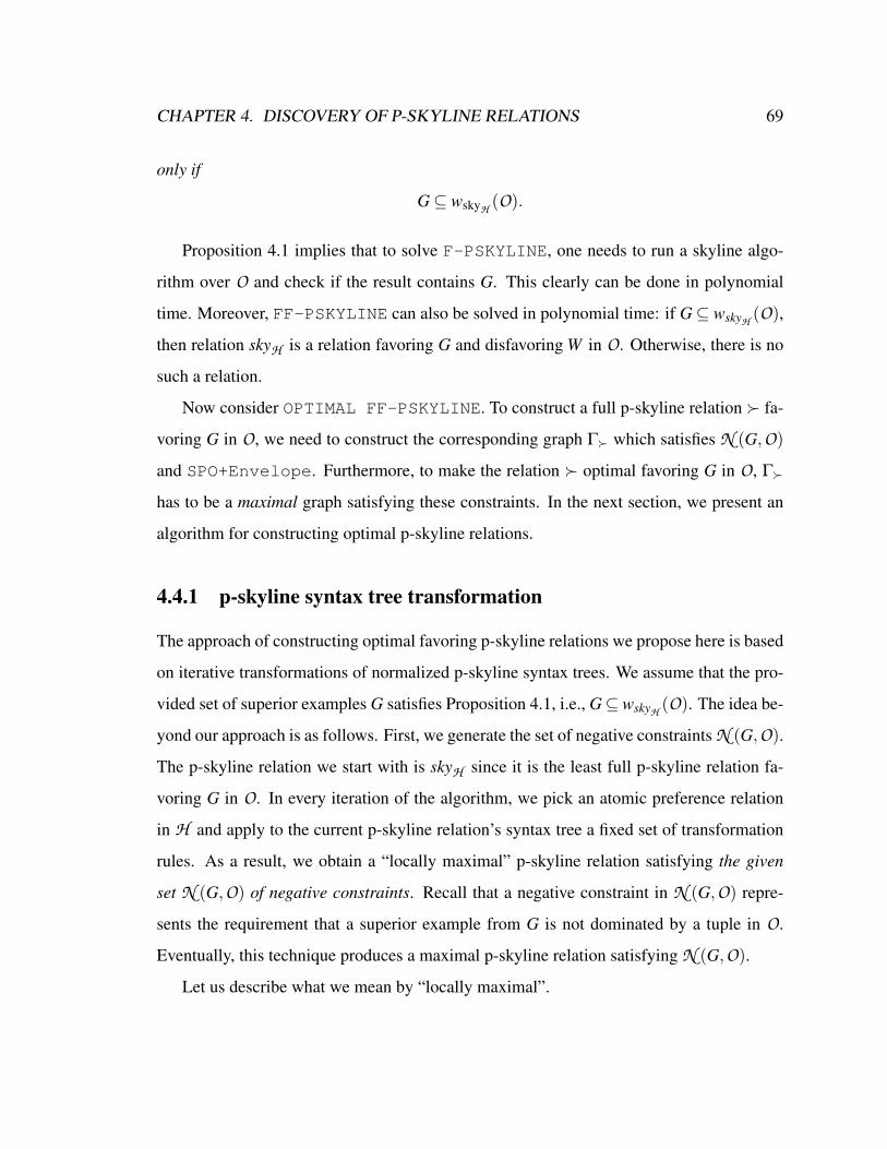
CHAPTER 4. DISCOVERY OF P-SKYLINE RELATIONS 69
only if
G⊆ wskyH (O).
Proposition 4.1 implies that to solve F-PSKYLINE, one needs to run a skyline algo-
rithm over O and check if the result contains G. This clearly can be done in polynomial
time. Moreover, FF-PSKYLINE can also be solved in polynomial time: if G⊆ wskyH (O),
then relation skyH is a relation favoring G and disfavoring W in O. Otherwise, there is no
such a relation.
Now consider OPTIMAL FF-PSKYLINE. To construct a full p-skyline relation fa-
voring G in O, we need to construct the corresponding graph Γ which satisfies N (G,O)
and SPO+Envelope. Furthermore, to make the relation optimal favoring G in O, Γ
has to be a maximal graph satisfying these constraints. In the next section, we present an
algorithm for constructing optimal p-skyline relations.
4.4.1 p-skyline syntax tree transformation
The approach of constructing optimal favoring p-skyline relations we propose here is based
on iterative transformations of normalized p-skyline syntax trees. We assume that the pro-
vided set of superior examples G satisfies Proposition 4.1, i.e., G⊆wskyH (O). The idea be-
yond our approach is as follows. First, we generate the set of negative constraints N (G,O).
The p-skyline relation we start with is skyH since it is the least full p-skyline relation fa-
voring G in O. In every iteration of the algorithm, we pick an atomic preference relation
in H and apply to the current p-skyline relation’s syntax tree a fixed set of transformation
rules. As a result, we obtain a “locally maximal” p-skyline relation satisfying the given
set N (G,O) of negative constraints. Recall that a negative constraint in N (G,O) repre-
sents the requirement that a superior example from G is not dominated by a tuple in O.
Eventually, this technique produces a maximal p-skyline relation satisfying N (G,O).
Let us describe what we mean by “locally maximal”.
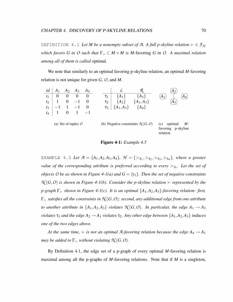
CHAPTER 4. DISCOVERY OF P-SKYLINE RELATIONS 70
DEFINITION 4.1 Let M be a nonempty subset of A . A full p-skyline relation ∈ FH
which favors G in O such that Γ ⊂M×M is M-favoring G in O. A maximal relation
among all of them is called optimal.
We note that similarly to an optimal favoring p-skyline relation, an optimal M-favoring
relation is not unique for given G, O, and M.
id A1 A2 A3 A4t1 0 0 0 0t2 1 0 −1 0t3 −1 1 −1 0t4 1 0 1 −1
(a) Set of tuples O
L Rτ1 A1 A3τ2 A2 A1,A3τ3 A1,A3 A4
(b) Negative constraints N (G,O)
A1
A2
A3
A4
(c) optimal M-favoring p-skylinerelation
Figure 4-1: Example 4.5
EXAMPLE 4.5 Let A = A1,A2,A3,A4, H = >A1,>A2,>A3,>A4, where a greater
value of the corresponding attribute is preferred according to every >Ai . Let the set of
objects O be as shown in Figure 4-1(a) and G = t1. Then the set of negative constraints
N (G,O) is shown in Figure 4-1(b). Consider the p-skyline relation represented by the
p-graph Γ shown in Figure 4-1(c). It is an optimal A1,A2,A3-favoring relation: first,
Γ satisfies all the constraints in N (G,O); second, any additional edge from one attribute
to another attribute in A1,A2,A3 violates N (G,O). In particular, the edge A1 → A3
violates τ1 and the edge A2→ A1 violates τ2. Any other edge between A1,A2,A3 induces
one of the two edges above.
At the same time, is not an optimal A-favoring relation because the edge A4→ A1
may be added to Γ without violating N (G,O).
By Definition 4.1, the edge set of a p-graph of every optimal M-favoring relation is
maximal among all the p-graphs of M-favoring relations. Note that if M is a singleton,

CHAPTER 4. DISCOVERY OF P-SKYLINE RELATIONS 71
the edge set of a p-graph Γ of an optimal M-favoring relation is empty, i.e., = skyH .
If M = A , then an optimal p-skyline relation M-favoring G in O is also an optimal p-
skyline relation favoring G in O. Thus, if we had a method of transforming an optimal
M-favoring to an optimal (M ∪ A)-favoring p-skyline relation for any attribute A, we
could construct an optimal favoring p-skyline relation by induction. A useful property of
such a transformation process is shown in the next lemma.
LEMMA 4.2 Let a full p-skyline relation ∈ FH be an optimal M-favoring relation, and
a full p-skyline extension ext of be (M∪A)-favoring. Then any edge in Γext −Γ
starts or ends in A.
PROOF
Take Γext and construct Γ′ from it by removing all edges going from and to A. Clearly,
Γ′ is an SPO. Now consider the Envelope property. Pick any four nodes of Γ different
from A. Since Γext is a p-graph, the Envelope property holds for the graph induced
by these four nodes in Γext . Assume it does not hold for the subgraph of Γ′ induced by
these nodes. That means that some edge between these four nodes is not present in Γ′
which means that some of these nodes was A, i.e., we get a contradiction. Thus, Γ′ satisfies
the Envelope property as well, i.e., it’s a p-graph of a p-skyline relation ′. Moreover,
Γ ⊆ Γ′ since Γ has no edges from/to A and Γ ⊆ Γext . Since is optimal M-favoring,
Γ = Γ′. Therefore, all edges in Γext −Γ go from or to A.
EXAMPLE 4.6 Consider N (G,O) from Example 4.5 also shown in Figure 4-2(a), and
the optimal A1,A2,A3-favoring relation. Several different optimal A-favoring p-skyline
relations which contain are possible here. Two of them are 1 and 2 whose p-graphs
are shown in Figures 4-2(b) and 4-2(c).
In section 3.6, we showed four syntax tree transformation rules which can be used to
extend a p-skyline relations in a minimal way. Although an optimal (M ∪A)-favoring
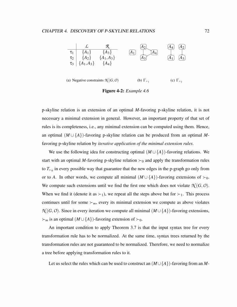
CHAPTER 4. DISCOVERY OF P-SKYLINE RELATIONS 72
L Rτ1 A1 A3τ2 A2 A1,A3τ3 A1,A3 A4
(a) Negative constraints N (G,O)
A1
A2
A3
A4
(b) Γ1
A1
A2
A3
A4
(c) Γ2
Figure 4-2: Example 4.6
p-skyline relation is an extension of an optimal M-favoring p-skyline relation, it is not
necessary a minimal extension in general. However, an important property of that set of
rules is its completeness, i.e., any minimal extension can be computed using them. Hence,
an optimal (M ∪ A)-favoring p-skyline relation can be produced from an optimal M-
favoring p-skyline relation by iterative application of the minimal extension rules.
We use the following idea for constructing optimal (M∪A)-favoring relations. We
start with an optimal M-favoring p-skyline relation 0 and apply the transformation rules
to T0 in every possible way that guarantee that the new edges in the p-graph go only from
or to A. In other words, we compute all minimal (M ∪A)-favoring extensions of 0.
We compute such extensions until we find the first one which does not violate N (G,O).
When we find it (denote it as 1), we repeat all the steps above but for 1. This process
continues until for some m, every its minimal extension we compute as above violates
N (G,O). Since in every iteration we compute all minimal (M∪A)-favoring extensions,
m is an optimal (M∪A)-favoring extension of 0.
An important condition to apply Theorem 3.7 is that the input syntax tree for every
transformation rule has to be normalized. At the same time, syntax trees returned by the
transformation rules are not guaranteed to be normalized. Therefore, we need to normalize
a tree before applying transformation rules to it.
Let us select the rules which can be used to construct an (M∪A)-favoring from an M-

CHAPTER 4. DISCOVERY OF P-SKYLINE RELATIONS 73
favoring p-skyline relations. By Lemma 4.2, such rules may add only such edges to p-graph
that go to A or from A. According to Observation 3.1, Rule1 adds edges going to the node
A if Ci+1 = A or N1 = A. Similarly, Rule2 adds edges going from A if Ci+1 = A or Nm = A.
Rule3 adds edges going from or to A if Ci = A or Ci+1 = A correspondingly. However,
Rule4 can only be applied to a pair of & -nodes. Hence, as we showed in section 3.6, that
rule adds edges going from at least two nodes to at least two different nodes of a p-graph.
Hence, any application of Rule4 violates Lemma 4.2. We conclude that Rule1,Rule2,Rule3
are sufficient to construct any optimal (M∪A)-favoring p-skyline relation.
4.4.2 Efficient constraint checking
Before going to details of the algorithm of p-skyline relation discovery we outlined in the
previous section, we consider an important step of the algorithm – testing if an extension
of a p-skyline relation satisfies a set negative constraints. In this section, we propose an
efficient method to do that.
Recall that a negative constraint is
τ : ChΓ(Lτ) 6⊇ Rτ
It can be visualized as two layers of nodes Lτ and Rτ. For any full p-skyline relation
∈ FH satisfying τ, its p-graph Γ may induce edges going between the nodes of the
layers Lτ and Rτ. However, in order for to satisfy τ, there should be at least one member
of Rτ with no incoming edges from Lτ.
The method of efficient checking negative constraints against a p-graph we propose
here is based on the fact that the edge set of the p-graph of a transformed p-skyline relation
monotonically increases. Therefore, while we transform a p-skyline relation , we can
simply drop the elements of Rτ which already have incoming edges from Lτ. If we do

CHAPTER 4. DISCOVERY OF P-SKYLINE RELATIONS 74
so after every transformation of the p-skyline relation , the negative constraint τ will be
violated by a Γ only if Rτ is empty. The next proposition says that such a modification of
negative constraints is valid.
PROPOSITION 4.2 Let a full p-skyline relation ∈ FH satisfy a system of negative
constraints N . Construct the system of negative constraints N ′ from N in which every
τ′ ∈N ′ is created from a member τ of N in the following way
• Lτ′ = Lτ
• Rτ′ = Rτ−Y ∈ Rτ | ∃X ∈ Lτ . (X ,Y ) ∈ Γ
Then any full p-skyline extension ′ of satisfies N if and only if ′ satisfies N ′.
A constraint τ′ constructed from τ as shown in Proposition 4.2 is called a minimal
negative constraints w.r.t. . The corresponding system of negative constraints N ′ is
called a minimal system of negative constraints w.r.t. .
PROOF OF PROPOSITION 4.2.
⇐ Take any τ′ from N ′ with the corresponding τ∈N . By construction, Lτ = Lτ,Rτ′ ⊆Rτ.
Now assume ′ satisfies τ′. This means that
∃B ∈ Rτ′ ∀A ∈ Lτ′ : (A,B) 6∈ Γ′ (4.5)
Now recall that Rτ′ ⊆ Rτ. Thus B ∈ Rτ. This together with Lτ = Lτ′ and (4.5) gives
∃B ∈ Rτ ∀A ∈ Lτ . (A,B) 6∈ Γ′,
i.e., Γ′ satisfies τ.
⇒ Now let ′ satisfy τ. This means
∃B ∈ Rτ ∀A ∈ Lτ . (A,B) 6∈ Γ′ (4.6)
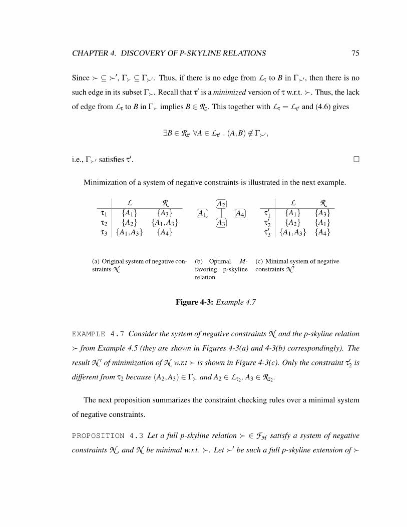
CHAPTER 4. DISCOVERY OF P-SKYLINE RELATIONS 75
Since ⊆ ′, Γ ⊆ Γ′ . Thus, if there is no edge from Lτ to B in Γ′ , then there is no
such edge in its subset Γ. Recall that τ′ is a minimized version of τ w.r.t. . Thus, the lack
of edge from Lτ to B in Γ implies B ∈ Rτ. This together with Lτ = Lτ′ and (4.6) gives
∃B ∈ Rτ′ ∀A ∈ Lτ′ . (A,B) 6∈ Γ′,
i.e., Γ′ satisfies τ′.
Minimization of a system of negative constraints is illustrated in the next example.
L Rτ1 A1 A3τ2 A2 A1,A3τ3 A1,A3 A4
(a) Original system of negative con-straints N
A1
A2
A3
A4
(b) Optimal M-favoring p-skylinerelation
L Rτ′1 A1 A3τ′2 A2 A1τ′3 A1,A3 A4
(c) Minimal system of negativeconstraints N ′
Figure 4-3: Example 4.7
EXAMPLE 4.7 Consider the system of negative constraints N and the p-skyline relation
from Example 4.5 (they are shown in Figures 4-3(a) and 4-3(b) correspondingly). The
result N ′ of minimization of N w.r.t is shown in Figure 4-3(c). Only the constraint τ′2 is
different from τ2 because (A2,A3) ∈ Γ and A2 ∈ Lτ2 , A3 ∈ Rτ2 .
The next proposition summarizes the constraint checking rules over a minimal system
of negative constraints.
PROPOSITION 4.3 Let a full p-skyline relation ∈ FH satisfy a system of negative
constraints N , and N be minimal w.r.t. . Let ′ be such a full p-skyline extension of

CHAPTER 4. DISCOVERY OF P-SKYLINE RELATIONS 76
that every edge in Γ′−Γ starts or ends in A. Denote the new parents and children of A
in Γ′ as PA and CA correspondingly. Then′ violates N if and only if there is a constraint
τ ∈N such that
1. Rτ = A∧PA∩Lτ 6= /0, or
2. A ∈ Lτ∧Rτ ⊆CA
PROOF
⇐ Trivial since the two conditions above imply violation of N ′ by .
⇒ Assume that there is no constraint τ for which the two conditions hold, but some τ′ ∈N
is violated, i.e.,
ChΓ(Lτ′)⊇ Rτ′ .
By Theorem 3.4, Γ ⊂ Γ′ . We also know that all the new edges in Γ′ start or end in A.
Since Γ satisfies τ′ but Γ′ does not, we get that either A ∈ Lτ′ or A ∈ Rτ′ . If A is in Rτ′
then the fact that τ′ is violated by Γ′ implies that Rτ′ = A. Moreover, the fact that τ′ is
minimal w.r.t. implies PA∩Lτ′ 6= /0. If A ∈ Lτ′ , then the minimality of τ′ implies that τ′
is violated because of Rτ′ ⊆CA.
Proposition 4.3 is illustrated in the next example.
EXAMPLE 4.8 Take the minimal system of negative constraints N ′ w.r.t. from Exam-
ple 4.7. Let us construct a full p-skyline extensions′ of such that every edge in Γ′−Γ
starts or ends in A4. Consider possible edges going to A4. We use Proposition 4.3 to check
if a new edge violates N ′. The edge (A1,A4) ∈ Γ′ is not allowed because A1 ∈ Lτ′3and
A4 = Rτ′3. The edge (A3,A4) ∈ Γ′ is not allowed because A3 ∈ Lτ′3
and A4 = Rτ′3.
However, the edge (A2,A4) ∈ Γ′ is allowed. The p-graph of the resulting ′ is shown in
Figure 4-4. One can analyze the edges going from A4 in a similar fashion.
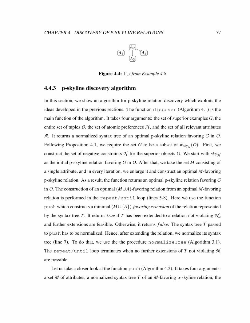
CHAPTER 4. DISCOVERY OF P-SKYLINE RELATIONS 77
A1
A2
A3
A4
Figure 4-4: Γ′ from Example 4.8
4.4.3 p-skyline discovery algorithm
In this section, we show an algorithm for p-skyline relation discovery which exploits the
ideas developed in the previous sections. The function discover (Algorithm 4.1) is the
main function of the algorithm. It takes four arguments: the set of superior examples G, the
entire set of tuples O, the set of atomic preferences H , and the set of all relevant attributes
A . It returns a normalized syntax tree of an optimal p-skyline relation favoring G in O.
Following Proposition 4.1, we require the set G to be a subset of wskyH (O). First, we
construct the set of negative constraints N for the superior objects G. We start with skyH
as the initial p-skyline relation favoring G in O. After that, we take the set M consisting of
a single attribute, and in every iteration, we enlarge it and construct an optimal M-favoring
p-skyline relation. As a result, the function returns an optimal p-skyline relation favoring G
in O. The construction of an optimal (M∪A)-favoring relation from an optimal M-favoring
relation is performed in the repeat/until loop (lines 5-8). Here we use the function
push which constructs a minimal (M∪A)-favoring extension of the relation represented
by the syntax tree T . It returns true if T has been extended to a relation not violating N ,
and further extensions are feasible. Otherwise, it returns f alse. The syntax tree T passed
to push has to be normalized. Hence, after extending the relation, we normalize its syntax
tree (line 7). To do that, we use the the procedure normalizeTree (Algorithm 3.1).
The repeat/until loop terminates when no further extensions of T not violating N
are possible.
Let us take a closer look at the function push (Algorithm 4.2). It takes four arguments:
a set M of attributes, a normalized syntax tree T of an M-favoring p-skyline relation, the

CHAPTER 4. DISCOVERY OF P-SKYLINE RELATIONS 78
Algorithm 4.1 discover(G, O, H , A)
Require: G⊆ wskyH (O)1: N = N (G,O)2: T = a normalized syntax tree of skyH3: M = set containing an arbitrary attribute from A4: for each attribute A in A−M do5: repeat6: r = push(T , M, A, N );7: normalizeTree(root of T );8: until r is false9: M = M∪A
10: end for11: return T
current attribute A, and a system of negative constraints N minimal w.r.t. ( here is a
p-skyline relation represented by the syntax tree T ). It returns true if a rewriting rule has
been applied to T without violating N , and f alse if no rewriting rule can be applied to T
without violating N . When the function returns, N is minimal w.r.t. the p-skyline relation
represented by the modified syntax tree, and T is normalized.
The goal of push is to find an appropriate rewriting rule which adds to the current
p-graph edges going from M to A or vice versa. The function has two branches: the parent
of the node A in the syntax tree T is a & -node (i.e., we may apply Rule1 where N1 is A
or Rule2 where Nm is A), or a ⊗ -node (i.e., we may apply Rule1 or Rule2 where Ci+1 is
A, or Rule3 where Ci or Ci+1 is A). In the first branch (line 2-14), we distinguish between
applying Rule1 (line 3-8) and Rule2 (line 9-14). It is easy to notice that with the parameters
specified above, the rules are exclusive. However, the application patterns are similar. First,
we find an appropriate child Ci+1 of R (lines 4 and 10). It is important for Var(Ci+1) to be
a subset of M because we want to add edges going from M to A or from A to M. Then
we check if the corresponding rule application will not violate N . To do that, we use the
function checkConstr (lines 5 and 11) as per Proposition 4.3. If a rule application does
not violate N , we apply the corresponding rule (lines 6 and 12) and minimize N w.r.t.

CHAPTER 4. DISCOVERY OF P-SKYLINE RELATIONS 79
the p-skyline which is the result of the rewriting (Proposition 4.2). To do that, we use the
function minimize.
The second branch of push is similar to the first one and different in only the rewriting
rules applied. As a result, it is easy to notice that push checks every possible rule applica-
tion not violating N and adds to the p-graph only the edges going from A to the elements
of M or vice versa.
In our implementation of the algorithm, all sets of attributes are represented as bitmaps
of fixed size |A |. Similarly, every negative constraint τ is represented as a pair of the
bitmaps corresponding to Lτ and Rτ. With every node Ci of the syntax tree, we associate a
variable storing Var(Ci). Its value is updated whenever the children list of Ci is changed.
THEOREM 4.4 The function discover returns a syntax tree of an optimal p-skyline
relation favoring G in O. Its runtime is O(|N | · |A |3).
PROOF
First, we prove that discover always returns a maximal p-skyline relation satisfying N .
By construction, a p-skyline relation returned by the function satisfies the system of nega-
tive constraints N constructed in discover. Now prove that returned by discover
is a maximal p-skyline relation satisfying N . A simple case analysis shows that push
picks every p-skyline relation which is
1. a minimal extension of represented by the parameter T , and
2. whose p-graph has only edges going between the nodes (M∪A),
until it finds one not violating N (of course, given the fact that ′, whose p-graph ob-
tained from Γ by removing edges going to/from A, is optimal M-favoring). Recall that
T computed in line 2 of discover represents a maximal M-favoring p-skyline relation
satisfying N , for a singleton M. Now assume that T at the end of some iteration of the
for-loop of discover represents a not maximal M-favoring p-skyline relation. Take the

CHAPTER 4. DISCOVERY OF P-SKYLINE RELATIONS 80
Algorithm 4.2 push(T , M, A, N )Require: T is normalized
1: if the parent of A in T is of type &2: Ci := parent of A in T ; R := parent of Ci in T ;3: if A is the first child of Ci4: for each child Ci+1 of R s.t. Var(Ci+1)⊆M5: if checkConstr(N , A, /0, Var(Ci+1))6: apply Rule1(T,Ci,Ci+1)7: N := minimize(N ,Var(A),Var(Ci+1))8: return true9: else if A is the last child of Ci
10: for each child Ci+1 of R s.t. Var(Ci+1)⊆M11: if checkConstr(N , A, Var(Ci+1), /0)12: apply Rule2(T,Ci,Ci+1)13: N := minimize(N ,Var(Ci+1),Var(A))14: return true15: else // the parent of A in T is of type ⊗16: R := parent of A in T ;17: for each child Ci of R s.t. Var(Ci)⊆M18: if Ci is of type &19: N1 := first child of Ci, Nm := last child of Ci20: if checkConstr(N , A, Var(N1), /0)21: apply Rule1(T,Ci,A)22: N :=minimize(N , Var(N1), Var(A))23: return true24: else if checkConstr(N , A, /0, Var(Nm))25: apply Rule2(T,Ci,A)26: N := minimize(N , Var(A), Var(Nm))27: return true28: else // Ci is a leaf node, since T is normalized29: if checkConstr(N , A, Var(Ci), /0)30: apply Rule3(T,Ci,A)31: N :=minimize(N , Var(Ci), Var(A))32: return true33: else if checkConstr(N , A, /0, Var(Ci)34: apply Rule3(T,A,Ci)35: N :=minimize(N , Var(A), Var(Ci))36: return true37: return f alse

CHAPTER 4. DISCOVERY OF P-SKYLINE RELATIONS 81
Algorithm 4.3 checkConstr(N , A, PA, CA)
for each τ ∈N doif Rτ = A∧PA∩Lτ 6= /0 or A ∈ Lτ∧Rτ ⊆CA then
return f alseend if
end forreturn true
Algorithm 4.4 minimize(N , U , D)
1: for each constraint τ in N do2: if U ∩Lτ 6= /0 then3: Rτ← Rτ−D4: end if5: end for6: return N
first such an iteration of the for-loop. It implies that there is ∗ which strictly contains
and satisfies N . By Theorem 3.4, Γ∗ also strictly contains Γ. Take an edge (X ,Y ) ∈ Γ∗
which is not in Γ. Let ′ be the relation computed in the for-loop in discover when A
was equal to X or Y , whatever was the last one. Take the corresponding set M. According
to the argument above, ′ is optimal M-favoring. Since ′ ⊆ , Γ′ does not contain the
edge from X to Y . At the same time, if we take Γ∗ and leave in it only the edges going
to and from the elements of M, it will strictly contain Γ′ and not violate N . Hence, ′ is
not optimal M-favoring, which is a contradiction. That implies that discover returns an
optimal A-favoring (or simply favoring) p-skyline relation satisfying N .
Now let us show that the runtime of the algorithm is O(|N | · |A |3). First, let us consider
the running time of the subprocedures. The runtime of minimize and checkConstr
is O(|N | · |A |). The time needed to modify the syntax tree using any transformation rule
is O(|A |): every rule creates, deletes, and modifies a constant number of nodes of a syn-
tax tree, but updating their Var-variables is done in O(|A |). Similarly, syntax tree nor-
malization runs in TnormalizeTree = O(|A |) for such modified syntax trees. As a result,

CHAPTER 4. DISCOVERY OF P-SKYLINE RELATIONS 82
S⊗start
S3
Rule3 S&
Rule1,Rule2 Rule1,Rule2
Figure 4-5: Using push for computation of an optimal (M∪A)-favoring p-skyline re-lation
the time needed to execute the bodies of the loops (lines 5-8, 11-14, 18-36) of push is
Trule = O(|N | · |A |).
Now let T be a syntax tree of an optimal M-favoring p-skyline relation. Now consider
the way push is used in discover to construct an optimal (M∪A)-favoring p-skyline
relation. The state diagram of this process is shown in Figure 4-5. It has three states: S⊗
and S& which correspond to T in which A is a child of a ⊗- and &-node, respectively; and
S3 which corresponds to the case when no rewriting rule can be applied to T , or any rule
application violates N .
The starting state is S⊗, because in the starting T , A is a child of the topmost ⊗-node.
After applying the rewriting rules Rule1 and Rule2 in lines 21 and 25 respectively, A be-
comes a child node of another ⊗-node of the modified T . After applying Rule3 (lines 30
and 34), A becomes a child of a &-node in the modified T , and we go to the state S&. When
in S&, we can only apply Rule1 or Rule2 from lines 6 and 12 respectively. Note that after
applying these rules, A is still a child of the same &-node in the modified T . When no rule
can be applied to T at any state, we go to the accepting state S3 and return f alse.
Consider the total number of nodes of T enumerated in the loops (lines 4-8, 10-14, and
17-36) of push to construct an optimal (M∪A)-favoring p-skyline relation. Note that
when we go from S⊗ to S⊗ by applying Rule1 or Rule2, A becomes a descendent of the
⊗-node whose child it was originally. Hence, when in S⊗ we enumerate the nodes Ci to

CHAPTER 4. DISCOVERY OF P-SKYLINE RELATIONS 83
apply Rule1 or Rule2 to, we never pick any Ci which we picked in the previous calls of
push. In the process of going from S& to itself via an application of Rule1 or Rule2, we
may enumerate the same node Ci+1 more than once because A does not change its parent &-
node as a result of these applications. To avoid checking these rules against the same nodes
Ci+1 more than once, one can keep track of the nodes which have already been picked and
tested.
Since the total number of nodes in a syntax tree is O(|A |), the tests Var(Ci+1)⊆M (lines
4, 10) and Var(Ci) ⊆M (line 17) are performed O(|A |) times and the rules are applied to
the tree O(|A |) times. Each of the containment tests above requires time O(|A |) given the
bitmap representation of sets. Hence, to compute the tree of an optimal (M∪A)-favoring
from the tree of an optimal M-favoring p-skyline relation, we need time O(|N | · |A |2).
Finally, the running time of discover is O(|N | · |A |3).
An important observation here is that the order in which the attributes are picked and
put to M in discover may be arbitrary. Moreover, the order of rules in which they are
applied in push may be also changed. That is, we currently try to apply Rule1 (line 21)
first and Rule2 (line 25) after it. However, one can apply them in the opposite order. The
same applies to Rule3(T,A,Ci) and Rule3(T,Ci,A) (lines 30 and 34, respectively). If any
of these parameters of the algorithm is changed, the generated p-skyline relation may be
different. However, even if it is different, it will still be an optimal favoring G in O. Note
also that due to the symmetry of ⊗ , the order of child nodes in a ⊗ may be different
in normalized p-skyline trees of equivalent p-skyline relations. Hence, the order in which
the leaf nodes are stored in the normalized syntax tree of skyH (line 2 of discover) also
affects the resulting p-skyline relation.
An example of applying Algorithm 4.1 is shown in the next section.

CHAPTER 4. DISCOVERY OF P-SKYLINE RELATIONS 84
4.4.4 Reducing the number of negative constraints
As we showed in Theorem 4.4, the runtime of the function discover linearly depends
on the size of the system of negative constraints N . If N = N (G,O), then it contains
(|O|−1) · |G| constraints. In this section, we propose two methods of reducing the size of
N . Both methods are based on applying the skyline operator. However, the first method
applies it to the tuple set O, and the second to the set of constraints itself.
Note that each negative constraint is used to show that a tuple should not be preferred to
a superior example. We also know that the relation skyH is the least full p-skyline relation.
By definition of the winnow operator, for every o′ ∈ O −wskyH (O) there is a tuple o ∈
wskyH (O) s.t. o is preferred to o′ according to skyH . Since skyH is the least full p-skyline
relation, the same o is preferred to o′ according to every full p-skyline relation. Thus, in
order to guarantee favoring G in O, the system of negative constraints needs to contain
only the constraints showing that the tuples in wskyH (O) are not preferred to the superior
examples. The size of such a system of negative constraints is (|wskyH (O)|−1) · |G|.
Another way to reduce the size of a system of negative constraints is based on the
following fact. Let us take two negative constraints τ,τ′ ∈N such that Lτ′ ⊆ Lτ, Rτ ⊆ Rτ′ ,
and let at least one of these relationships be strict. It is easy to check that τ strictly implies
τ′. Thus, the constraint τ′ is redundant and may be deleted from N . This idea can also be
expressed as follows:
τ strictly implies τ′ if and only if Lτ′ ⊆ Lτ∧ (A−Rτ′)⊆ (A−Rτ)
and at least one containment is strict
Let us represent τ as a bitmap representing (A−Rτ) appended to a bitmap representing Lτ.
We assume that a bit is set to 1 iff the corresponding attribute is in the corresponding set.
Denote such a representation as bitmap(τ).

CHAPTER 4. DISCOVERY OF P-SKYLINE RELATIONS 85
EXAMPLE 4.9 Let Lτ = A1,A3,A5, Rτ = A2, Lτ′ = A1,A5, Rτ′ = A2,A4. Let
A = A1, . . . ,A5. Then bitmap(τ) = 10101 10111 and bitmap(τ′) = 10001 10101.
Consider bitmap(τ) as a vector with 2 · |A | dimensions. From the negative constraint
implication rule, it follows that τ strictly implies τ′ iff bitmap(τ) and bitmap(τ′) satisfy the
Pareto improvement principle, i.e., the value of every dimension of bitmap(τ) is greater
or equal to the corresponding value in bitmap(τ), and there is at least one dimension
whose value in bitmap(τ) is greater than in bitmap(τ′). Therefore, the set of all non-
redundant constraints in N corresponds to the skyline of the set of bitmap representations
of all constraints in N . Moveover, bitmap(τ) can have only two values in every dimension.
Thus, an algorithm for computing skylines over low cardinality domains (e.g. [MPJ07]) can
be used to compute the set of non-redundant constraints.
⊗
price make year
(a)
⊗
& year
price make
(b)
&
⊗price
make year
(c)
&
price yearmake
(d)
Figure 4-6: Example 4.10
EXAMPLE 4.10 Take O and H from Example 4.1, and G from Example 4.3. Then the
corresponding system of negative constraints N (G,O) (Example 4.3) is
τ1 : t1 6 t3 ChΓ(make) 6⊇ price
τ2 : t2 6 t3 ChΓ(make,year) 6⊇ price
τ3 : t4 6 t3 ChΓ(make,year) 6⊇ price
τ4 : t5 6 t3 ChΓ(make) 6⊇ price,year
Let us find an optimal ∈ FH favoring G in O by running discover. Among the
constraints above, only N = τ2 : ChΓ(make, year) 6⊇ price is nonredundant.
CHAPTER 4. DISCOVERY OF P-SKYLINE RELATIONS 86
Moreover, it cannot be further minimized because Rτ is a singleton. Consider the attributes
in the order: make, price, and year.
We run discover. The tree T (line 2) is shown in Figure 4-6(a). The initial value
of M is make. First, we call push(T,M,price,N ). The parent of price is the ⊗-
node (Figure 4-6(a)), so we go to line 16 of push, where R is set to the ⊗-node (Figure
4-6(a)). After Ci is set to the node make in line 17, we go to line 29 because it is a leaf
node. The checkConstr test in line 29 fails because N prohibits the edge make→
price. Hence, we go to line 33 where the checkConstr test succeeds. We apply
Rule3(T,price,Ci), push returns true, and the resulting syntax tree T is shown in Figure
4-6(b). Next time we call push(T,M,price,N ) (line 6 of discover), we get to line 4
of push. Since year 6∈M, we immediately go to line 37 and return f alse. In discover
we set M to make,price and call push(T,M,year,N ). There we go to line 16 (R
is set to the ⊗-node in Figure 4-6(b)), Ci is set to the &-node (Figure 4-6(b)), we apply
Rule1(T,Ci,year) (the resulting tree T is show in Figure 4-6(c)), and true is returned.
When push(T,M,year,N ) is called next time, we first go to line 16, R is set to the⊗-node
(Figure 4-6(c)), and Ci to the node make. Then Rule3(T,Ci,year) is applied (line 30)
resulting in the tree T shown in Figure 4-6(d), and true is returned. push(T,M,year,N )
is called once again from discover, but it returns f alse, and thus the tree in Figure
4-6(d) is the final one. According to the corresponding p-skyline relation, t3 dominates all
other tuples in O.
The final p-skyline relation constructed in Example 4.10 is a prioritized accumulation
of all the atomic preference relations. This is due to the fact that N contained only one
constraint. When more constraints are involved, a discovered p-skyline relation generally
also has occurrences of Pareto accumulation.

CHAPTER 4. DISCOVERY OF P-SKYLINE RELATIONS 87
4.5 Experiments
We have performed extensive experimental study of the proposed framework. The algo-
rithms were implemented in Java. The experiments were ran on Intel Core 2 Duo CPU 2.1
GHz with 2.0GB RAM. The experiments were run on four data sets: one real life and three
synthetic.
4.5.1 Experiments with real life data
In this section, we focus on experimenting with the accuracy of the p-skyline relation dis-
covery algorithm and the reduction of skylines achieved by modeling user preferences using
p-skyline relations. We used a data set O which stores statistics of NHL players [nhl08]
containing 9395 tuples. We used three sets of relevant attributes A of 12, 9, and 6 attributes,
respectively. The sizes of the corresponding skylines were 568, 114, and 33.
Accuracy of p-skyline relation discovery
The aim of the first experiment is to demonstrate that the proposed p-skyline discovery
algorithm has a high accuracy. We use the following scenario here. We assume that pref-
erences of a user are modeled as a p-skyline relation, denoted as f av. We assume that
the user provides the set of relevant attributes A , the corresponding atomic preferences H ,
and a set G f av of tuples which she likes most in O (i.e., G f av are superior examples and
G f av ⊆ w f av(O)). We use G f av to compute an optimal p-skyline relation favoring G f av
in O. To measure the accuracy of the p-skyline relation discovery algorithm, we compare
the set of the best tuples w(O) in O according to the computed p-skyline relation with
the set of the best tuples w f av(O) in O according to the preference relation f av (which,
as we assumed, correctly describes the user preferences).
To model user preferences, we randomly generated 100 p-skyline relations f av. For
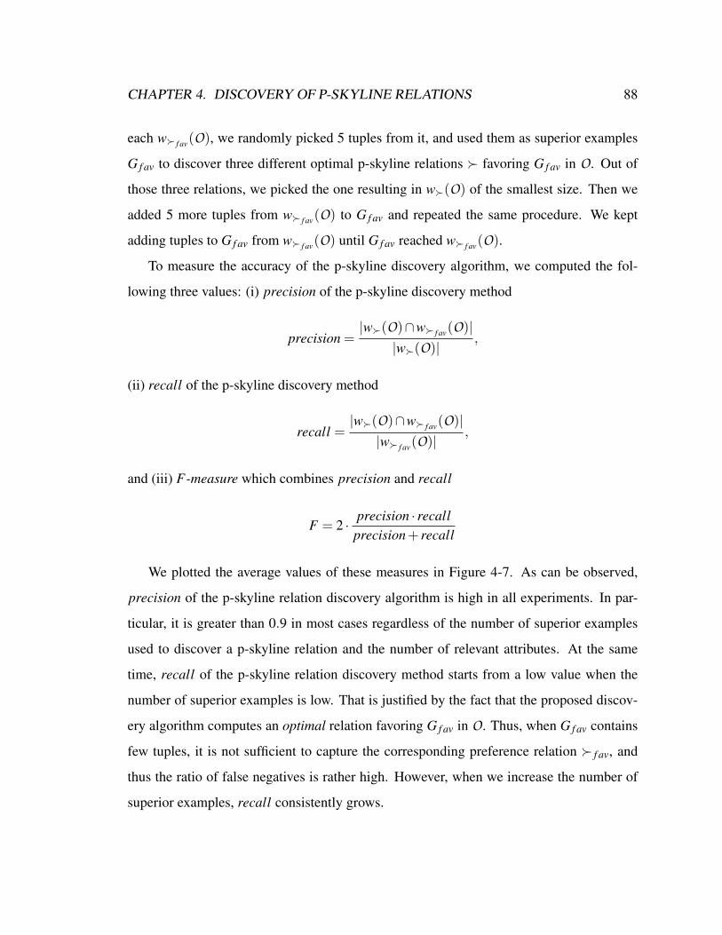
CHAPTER 4. DISCOVERY OF P-SKYLINE RELATIONS 88
each w f av(O), we randomly picked 5 tuples from it, and used them as superior examples
G f av to discover three different optimal p-skyline relations favoring G f av in O. Out of
those three relations, we picked the one resulting in w(O) of the smallest size. Then we
added 5 more tuples from w f av(O) to G f av and repeated the same procedure. We kept
adding tuples to G f av from w f av(O) until G f av reached w f av(O).
To measure the accuracy of the p-skyline discovery algorithm, we computed the fol-
lowing three values: (i) precision of the p-skyline discovery method
precision =|w(O)∩w f av(O)|
|w(O)|,
(ii) recall of the p-skyline discovery method
recall =|w(O)∩w f av(O)||w f av(O)|
,
and (iii) F-measure which combines precision and recall
F = 2 · precision · recallprecision+ recall
We plotted the average values of these measures in Figure 4-7. As can be observed,
precision of the p-skyline relation discovery algorithm is high in all experiments. In par-
ticular, it is greater than 0.9 in most cases regardless of the number of superior examples
used to discover a p-skyline relation and the number of relevant attributes. At the same
time, recall of the p-skyline relation discovery method starts from a low value when the
number of superior examples is low. That is justified by the fact that the proposed discov-
ery algorithm computes an optimal relation favoring G f av in O. Thus, when G f av contains
few tuples, it is not sufficient to capture the corresponding preference relation f av, and
thus the ratio of false negatives is rather high. However, when we increase the number of
superior examples, recall consistently grows.

CHAPTER 4. DISCOVERY OF P-SKYLINE RELATIONS 89
5 10 15 20 25 300.6
0.7
0.8
0.9
1
# superior examples
precision recall F
(a) |A |= 6
0 20 40 60 80
0.8
0.9
1
# superior examples
precision recall F
(b) |A |= 9
0 20 40 60 80 100
0.7
0.8
0.9
1
# superior examples
precision recall F
(c) |A |= 12
Figure 4-7: Accuracy of p-skyline discovery
In Figure 4-8, we plot the value of F-measure with respect to the share of the skyline
used as superior examples to discover the relation . As one can observe, the value of F
starts from a comparatively low value of 0.7 but quickly reaches 0.9 via a small increase
of the size of G f av. Another important observation is that the value of F is generally
inversely dependent on the number of relevant attributes (given the same ratio of superior
examples used). This is justified by the following fact. In order to compute a p-skyline
relation favoring G f av in O, the algorithm uses a set of negative constraints N . Intuitively,
the computed p-skyline relation will match the original relation f av better if the set N
“describes” f av sufficiently well. The number of constraints in N depends not only on the
number of superior examples but also on the total number of tuples in the corresponding
skyline. Since skyline sizes are generally smaller for smaller sets of A , more superior
objects are needed for smaller A to “describe” f av.
Reduction of size of winnow query result
In Section 3.8, we described a well known deficiency of the skyline framework – skylines
are generally of large size for large sets of relevant attributes. The goal of the experiments in
this section is twofold. First, we demonstrate that using p-skyline relations to model user
preferences results in smaller winnow query results in comparison to skylines. Second,
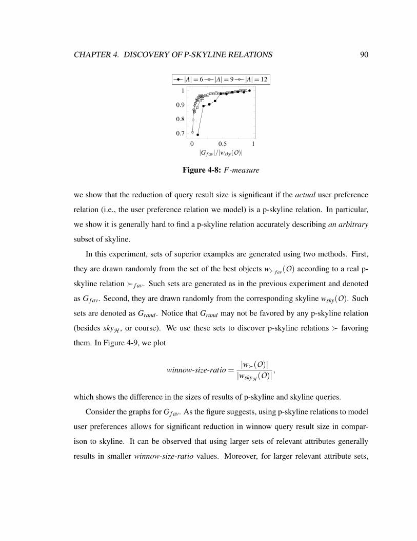
CHAPTER 4. DISCOVERY OF P-SKYLINE RELATIONS 90
0 0.5 1
0.7
0.8
0.9
1
|G f av|/|wsky(O)|
|A|= 6 |A|= 9 |A|= 12
Figure 4-8: F-measure
we show that the reduction of query result size is significant if the actual user preference
relation (i.e., the user preference relation we model) is a p-skyline relation. In particular,
we show it is generally hard to find a p-skyline relation accurately describing an arbitrary
subset of skyline.
In this experiment, sets of superior examples are generated using two methods. First,
they are drawn randomly from the set of the best objects w f av(O) according to a real p-
skyline relation f av. Such sets are generated as in the previous experiment and denoted
as G f av. Second, they are drawn randomly from the corresponding skyline wsky(O). Such
sets are denoted as Grand . Notice that Grand may not be favored by any p-skyline relation
(besides skyH , or course). We use these sets to discover p-skyline relations favoring
them. In Figure 4-9, we plot
winnow-size-ratio =|w(O)||wskyH (O)|
,
which shows the difference in the sizes of results of p-skyline and skyline queries.
Consider the graphs for G f av. As the figure suggests, using p-skyline relations to model
user preferences allows for significant reduction in winnow query result size in compar-
ison to skyline. It can be observed that using larger sets of relevant attributes generally
results in smaller winnow-size-ratio values. Moreover, for larger relevant attribute sets,
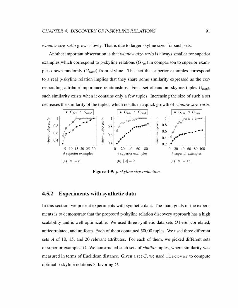
CHAPTER 4. DISCOVERY OF P-SKYLINE RELATIONS 91
winnow-size-ratio grows slowly. That is due to larger skyline sizes for such sets.
Another important observation is that winnow-size-ratio is always smaller for superior
examples which correspond to p-skyline relations (G f av) in comparison to superior exam-
ples drawn randomly (Grand) from skyline. The fact that superior examples correspond
to a real p-skyline relation implies that they share some similarity expressed as the cor-
responding attribute importance relationships. For a set of random skyline tuples Grand ,
such similarity exists when it contains only a few tuples. Increasing the size of such a set
decreases the similarity of the tuples, which results in a quick growth of winnow-size-ratio.
5 10 15 20 25 30
0.4
0.6
0.8
1
# superior examples
win
now
-siz
e-ra
tio
G f av Grand
(a) |A |= 6
0 20 40 60 80
0.4
0.6
0.8
1
# superior examples
win
now
-siz
e-ra
tio
G f av Grand
(b) |A |= 9
0 20 40 60 80 1000.2
0.4
0.6
0.8
1
# superior examplesw
inno
w-s
ize-
rati
o
G f av Grand
(c) |A |= 12
Figure 4-9: p-skyline size reduction
4.5.2 Experiments with synthetic data
In this section, we present experiments with synthetic data. The main goals of the experi-
ments is to demonstrate that the proposed p-skyline relation discovery approach has a high
scalability and is well optimizable. We used three synthetic data sets O here: correlated,
anticorrelated, and uniform. Each of them contained 50000 tuples. We used three different
sets A of 10, 15, and 20 relevant attributes. For each of them, we picked different sets
of superior examples G. We constructed such sets of similar tuples, where similarity was
measured in terms of Euclidean distance. Given a set G, we used discover to compute
optimal p-skyline relations favoring G.

CHAPTER 4. DISCOVERY OF P-SKYLINE RELATIONS 92
Scalability of p-skyline discovery
In this section, we show that the algorithm we proposed for p-skyline relation discovery
is scalable with respect to various parameters of the algorithm. In Figure 4-10, we plot
dependency of the average running time of discover on the number of superior examples
|G| used to discover a p-skyline relation (Figure 4-10(a), |O| = 50000, |A | = 20), the size
of O (Figure 4-10(b), |G|= 50, |A |= 20), and the number |A | of relevant attributes (Figure
4-10(c), |O|= 50000, |G|= 50). The measured time does not include the time to construct
the system of negative constraints and find the non-redundant constraints in it. According
to our experiments, the preprocessing time predominantly depends on the performance of
the skyline computation algorithm.
According to Figure 4-10(a), the algorithm running time increases until the size of G
reaches 30. After that, it does not vary much. This is due to the fact that the algorithm per-
formance depends on the number of used negative constraints. We use only non-redundant
constraints for discovery. As we show further, the dependence of the size of a system
of non-redundant constraints on the number of superior examples has a pattern similar to
Figure 4-10(a).
The growth of running time with the increase in the data set size (Figure 4-10(a)) is jus-
tified by the fact that the number of negative constraints depends on skyline size (Section
4.4.4). For the data sets used in the experiment, skyline sizes grow with the sizes of the
corresponding data sets. Similarly, the running time of the algorithm grows with the num-
ber of relevant attributes (Figure 4-10(c)) due to the increase in the corresponding skyline
size.
We conclude that the the running time of the algorithm for p-skyline discovery we have
proposed in this chapter has a low running time and scales well with respect to the number
of superior examples, the size of the data set, and the number of relevant attributes used in
discovery.

CHAPTER 4. DISCOVERY OF P-SKYLINE RELATIONS 93
0 50 100 150100
101
102
103
# superior examples
ms
anticorr uniformcorr
(a) against # superior examples
2 4·104
101
102
data set size
ms
anticorr uniformcorr
(b) against data set size
10 15 20
100
101
102
103
|A |
ms
anticorr uniformcorr
(c) against |A |
Figure 4-10: Performance of p-skyline discovery
Reduction in the number of negative constraints
In this section, we demonstrate that the proposed approach for p-skyline relation discovery
is well optimizable. We showed that the running time of discover linearly depends on
the number of negative constraints in the system N . Here we show that the techniques
proposed in Section 4.4.4 allow for significant reduction in the size of N .
In Figure 4-11(a), we show how the number of negative constraints depends on the num-
ber of superior examples used to construct them. For every data set, we plot two values: the
number of unique negative constraints in N (G,wskyH (O)) (anticorr-un, uni f orm-un, and
corr-un, resp.) and the number of unique non-redundant constraints in the corresponding
system (anticorr-nrd, uni f orm-nrd, and corr-nrd, resp.). We note that the reduction in the
constraint number achieved using the methods we proposed in Section 4.4.4 is significant.
In particular, for the anticorrelated data set and G of size 150, the total number of con-
straints in N (G,O) was approximately 7.5 ·106. Among them, about 5.5 ·106 were unique
in N (G,wskyH (O)). However, less than 1% of them (about 12 ·103) were non-redundant.

CHAPTER 4. DISCOVERY OF P-SKYLINE RELATIONS 94
Reduction of size of winnow query result
In Section 4.5.1, we showed how that the size of p-skyline preference query result depends
on the number of relevant attributes and the size of skyline. In this section, we show that
another parameter which affects winnow query size is the data distribution. In Figure 4-
11(b), we show how the size of the p-skyline query result varies with the number of superior
examples used to discover a p-skyline relation . We compare it with the size of the cor-
responding skyline and plot the value of winnow-size-ratio defined in the previous section.
Here we used the anticorrelated, the uniform, and the correlated data sets of 50000 tuples
each. The numbers of relevant attributes were 20. The sizes of the corresponding skylines
were: 41716 (anticorrelated), 37019 (uniform), and 33888 (correlated). For the anticorre-
lated and the uniform data sets, values of winnow-size-ratio quickly reach a certain bound
and then grow slowly with the number of superior examples. This bound is approximately
1% of the skyline size (i.e., about 350 tuples) for both data sets. At the same time, the
growth of winnow-size-ratio for the correlated data set is faster. Note that the values of
winnow-size-ratio are generally lower for synthetic data sets in comparison to the real life
data set in the previous section. This is due to the larger set of relevant attributes and larger
skyline sizes in the current experiment.
0 50 100 150
102
104
106
# superior examples
anticorr-un anticorr-nrduni f orm-un uni f orm-nrd
corr-un corr-nrd
(a) Constraint number reduction
0 50 100 150
10−2
10−1
100
# superior examples
win
now
-siz
e-ra
tio
anticorruniform
corr
(b) p-skyline size reduction
Figure 4-11: Synthetic data experiments

CHAPTER 4. DISCOVERY OF P-SKYLINE RELATIONS 95
We conclude that the experiments we carried out show that incorporating attribute im-
portance into skyline relations allows for significant reduction in query result size. The
algorithm for p-skyline relation discovery has good scalability in terms of data set size and
number of relevant attributes. The algorithm has a high accuracy even for small sets of
superior examples used to discover p-skyline relations.
4.6 Related work
An approach of mining preferences aggregated using the accumulation operators was pro-
posed by Holland et al in [HEK03]. Web server logs were used there to mine preference
relations. The mining approach is based on statistical properties of log data – more prefer-
able tuples appear more frequently. The process of mining user preferences is split into
two parts: mining atomic preferences and mining the accumulation operators connecting
the atomic preferences. Atomic preferences are mined in the form of the set of predefined
preference constructors such as LOWEST, HIGHEST etc. Categorical domain preferences
are mined in the form of simple constructors like POS, NEG as well as arbitrary strict partial
order relations. In order to mine preference relations aggregating atomic preferences us-
ing Pareto and prioritized accumulation operators, [HEK03] proposed a heuristic approach
based on associative rule mining. The cases when more than one different combination of
accumulation operators may be mined on the same data were not addressed. Moreover, no
criteria of optimality of mined preference relations were defined.
A framework of preference discovery which is a complementary to the approach we
have proposed here was presented by Jiang et al in [JPL+08]. In that work, preferences are
modeled as skyline relations. Given a set of relevant attributes and a set of atomic pref-
erences over some of them, the problem addressed there is computing atomic preferences
over the remaining attributes. The mining process is based on user feedback in terms of a
set of superior and a set of inferior examples. The focus of that work is to mine minimal (in
CHAPTER 4. DISCOVERY OF P-SKYLINE RELATIONS 96
terms of relation size) attribute preference relations. It was shown there that the problem of
existence of such relations is NP-complete in general, and the computation problem is in
general NP-hard. Two heuristic algorithms for computing such preferences were provided.
The algorithms are greedy and not sound, i.e., for some inputs, the computed preferences
may be not minimal. That approach and the approach we presented here are different in the
following sense. First, [JPL+08] deals with skyline relations, and thus all attribute pref-
erences are considered to be equally important. In contrast, the focus of our work is to
discover differences in attribute importance. Second, [JPL+08] focuses on mining minimal
attribute preferences. In contrast, we are interested in computing maximal preference rela-
tions since they guarantees a better fit to a provided set of superior examples. At the same
time, our work and [JPL+08] complement each other. Namely, when attribute preferences
are not provided explicitly be user, the approach [JPL+08] may be used to discover them.
Another approach of preference relation discovery in the skyline framework was pro-
posed by Lee et al in [LwYwH+08]. That work is motivated by the problem of large
skyline sizes. It proposes to reduce skyline sizes by revising skyline preference relations
by supplying additional tuple relationships: preference and equivalence. The relationships
are obtained from user’s answers to simple questions: 1) is an object preferred to another
object or vice versa, and 2) are two objects equivalent. [LwYwH+08] also developed an
algorithm that given a number k computes a minimal set of questions such that positive
answers to them result in the winnow query size at most k.
In quantitative preference frameworks [Fis70], preferences are represented as utility
functions: a tuple t is considered to be preferred to another tuple t ′ if f (t) > f (t ′) for a
utility function f . Attribute priorities are often represented here as weight coefficients in
polynomial utility functions. A number of methods have been proposed to elicit such utility
functions [CKP00, Bou02, GW05].
Representing preferences as utility functions was shown to be a powerful tool to reason

CHAPTER 4. DISCOVERY OF P-SKYLINE RELATIONS 97
as well as query databases with preferences [DFP03, BG96, FLN01, DGKT06]. Hence,
some work has been performed to eliciting utility functions for preferences represented
in other models. In [MD02], preferences are considered over finite domains and under
the ceteris paribus semantics. That work introduces a two-step algorithm for computing
a utility function representing a set of preference statements. It has the following steps:
(i) convert the statements to a special graph, and (i) use an appropriate class of a utility
function to represent the graph. [MD02] introduced four classes of such utility functions
with different properties.
Another model of preference elicitation in the form of utility functions was introduced
by Domshlak et al in [DJ07]. That work shows a framework of computing a utility func-
tion consistent with a set of comparative (e.g., “A is better than B” or “A is as good as
B”) statements about preferences. [DJ07] also mentions that the model can also handle
classificatory (e.g., “A is good”, “B is bad”) statements. That approach does not rely on
any structure of preference relations. In contrast to the majority of works in this area,
preferences over attributes here are not required to be independent, and the interpretations
of preference statements is not fixed and is one of the parameters of the elicitation algo-
rithm. The key idea of the framework is to map preference statements about tuples into
similar statements about higher dimensional tuples. The dimensionality extension is used
to capture the dependence of attribute preferences. After that, the corresponding statements
are converted to linear inequality constraints, and machine learning techniques are used to
efficiently compute a function satisfying the constraints.
In [VH99], Ha et al proposed an approach of composing binary preference relations
and utility functions of the class of multi-linear utility functions. They convert preference
instances of this class into inequality constraints, use Convex Cone Analysis to compute a
finite representation of the the resulting preference relations, and propose an algorithm for
reasoning with such preferences.

CHAPTER 4. DISCOVERY OF P-SKYLINE RELATIONS 98
A quantitative framework of eliciting binary preference relations was presented by Had-
dawy et al in [HRGM03]. Preferences here are elicited as a knowledge based artificial
neural network (KBANN). Prior knowledge of user preferences in terms of pairs of com-
parative tuple statements is encoded into a network as link weights. A network has 2n
inputs (where n is the number of attributes in a tuple) on which it takes the values of at-
tributes of two tuples to compare. It outputs a binary value: 1 if the first tuple is preferred
to the second, and 0 otherwise. However, properties of the binary relations induced by such
networks are not studied in this work. In particular, it is not clear if such relations are SPO.
To train a network, a wide range of types of data may be used: numeric ratings, pairwise
comparisons etc. [HRGM03] presents an experimental evaluation of the framework and
shows its effectiveness.
A number of incremental preference elicitation frameworks based on example critique
were proposed [LHL97, SL01, VFP06]. This class of frameworks generally uses the fol-
lowing scenario. An Agent starts with little or no information about preferences of the
User. In every iteration, the Agent shows to the user a carefully selected set of optimal
tuples based on the User preferences learned so far. After that, the User selects the tuples
in the set which she does not like and describes what exactly she does not like in them.
Given that knowledge, the Agent recomputes the model representing the preferences of the
User and goes to the next iteration. This process terminates when the User is completely
satisfied with the set of tuples. Preferences in such frameworks are generally represented as
utility functions. An important aspect of such systems is the type of user critiques collected
from the User and the user interface used to gather such information.
The discussion of the framework of p-skyline relation discovery based on superior/inferior
examples which we presented in this chapter is an extended version of our paper [MC09].
Chapter 5Hierarchical CP-nets
In this chapter, we propose the framework of hierarchical CP-nets (HCP-nets). It is a variant
of CP-nets which addresses some problems of the original framework. First, conditionality
of preferences over attributes in HCP-nets induces difference in the relative importance
of them, which is not always the case in CP-nets. Second, orders induced by HCP-nets
are succinctly representable as preference formulas, which is an open question for CP-net.
Third, HCP-nets can deal with finite as well as infinite domains, whilst CP-nets are defined
for finite domains.
5.1 CP-network framework
The CP-network framework was initially proposed in [BBHP99]. In this approach, prefer-
ences can be represented as conditional preference graphs. The nodes of such graphs are
attributes, i.e. members of A , and the edges are used to show that a preference over an
attribute is conditioned on the values of its parents in the graph. The framework can be
defined as follows.
The domains of all attributes A in this framework are considered to be finite. The
key notion is the conditional preference table. Given an attribute A ∈ A , the conditional
99

CHAPTER 5. HIERARCHICAL CP-NETS 100
preference table (or CPT) of A is
CPTA = (ΦA,UA),
where UA ⊆ A−A and ΦA = q1, . . . ,qk. Semantically, UA is a set of the attributes that
preferences over A are conditioned on, and ΦA is a set of conditional preference statements
over A. Every q in ΦA is defined as uq : Rq where uq ∈UUA , and Rq is a total order over
DA. Semantically, uq is a conditional part of q, while Rq is a preferential part of q. We also
assume that
• for every u ∈UUA , there is q ∈ΦA such that uq = u;
• for every pair of different q1,q2 ∈ΦA, we have uq1 6= uq2 .
The order induced by q ∈ΦA is defined as
q∗ = (o,o′) | o.UA = o′.UA = uq∧ (o.A,o′.A) ∈ Rq∧o.YA = o′.YA,
where YA = A − (A∪WA). In other words, a tuple o is preferred to a tuple o′ according
to q∗ if o.A is preferred to o′.A according to Rq, the values of UA in both tuples are equal
to uϕ and the values of the remaining attributes are pairwise equal. Note that for every pair
of objects (o,o′) ∈ q∗, o and o′ are different only in A. The principle of comparing objects
which are different in a single attribute is commonly referred as ceteris paribus.
The order induced by a conditional preference table CPTA is defined as
CPT ∗A =⋃
q∈ΦA
q∗
A CP-net is defined as N = CPTA | A ∈ A. The order N induced by a CP-net N is

CHAPTER 5. HIERARCHICAL CP-NETS 101
make
color
makeGM Ford
make colorGM red blueFord blue red
(a) ϒN1
(GM,red)
(GM,blue)
(Ford,blue)
(Ford,red)
(b) Dominance according to N1
Figure 5-1: CP-net from Example 5.1
defined as shown below. A CP-net is called consistent if it induces an SPO.
N= TC(⋃
A∈ACPT ∗A ).
The representation of a CP-net N as a conditional preference graph ϒN is defined as
follows. ϒN is a directed graph whose nodes are attributes, i.e., members of A . Every node
A is annotated with the corresponding conditional preference table and has incoming edges
from every member of UA. Although cyclicity of such a graph does not necessary imply
inconsistency of the corresponding CP-net, we consider CP-nets with acyclic graphs only.
EXAMPLE 5.1 Consider a CP-net N1 representing preferences over cars with two at-
tributes: make and color. Mary prefers GM to Ford. Given two GM cars, she prefers
the red car to the blue car. Given two Ford cars, she prefers the blue one to the red one.
The corresponding CP-net N1 can be represented by the conditional preference graph ϒN1
shown in Figure 5-1(a). In Figure 5-1(b), we show the order induced by N1.
5.1.1 Attribute importance in CP-nets
One of the main concepts of the CP-net framework is the conditionality of preferences over
an attribute on the values of a set of attributes. It was pointed out in [BBD+04] that a pos-

CHAPTER 5. HIERARCHICAL CP-NETS 102
sible reason for a user to have conditional preferences is a difference in relative importance
of attributes. Take a preference statement from Example 5.1: Mary prefers GM to Ford,
and given two GM with different colors, the red one is preferred to the blue one. One way
of interpreting this sentence is that given a set of cars, their make should be considered
first; and only when no benefits in make can be achieved, their colors have to be examined.
With such an interpretation, an edge from make to color in a conditional preference graph
also implies that the attribute make is more important than the attribute color. For instance,
according to N1 (Example 5.1), every GM is preferred to every Ford regardless of color.
However, as also noted in [BBD+04], such attribute importance relationships do not always
hold. Example 5.2 illustrates such a case.
EXAMPLE 5.2 Consider the CP-net N1 in Example 5.1. We extend it by expressing ad-
ditional preferences over car size: given two red cars, Mary prefers the smaller one; while
between two blue cars, she prefers the larger one. The resulting CP-net N2 is shown in
Figure 5-2(a), and the order induced by N2 is in Figure 5-2(b) (transitive preference edges
are skipped for clarity). Note that (GM,red,small) 6N2 (Ford,blue, large).
As can be observed from Example 5.2, not every GM is preferred to every Ford despite
the fact that make is the topmost node in the conditional preference graph. The reason is
that due to the ceteris paribus semantics of CP-nets, one tuple o is preferred to another o′ if
and only if there is a chain of tuples o = o1,o2, . . . ,ok−1,ok = o′ (called flipping sequence
[BBHP99]) such that for every i ∈ [1,k− 1], oi is preferred to oi+1 according to the order
CPT ∗A induced by the conditional preference table CPTA of some attribute A. Moreover,
each oi and oi+1 must be different in the value of A only. As Figure 5-2(b) shows, no such
a sequence exists for the pair of tuples shown in Example 5.2.

CHAPTER 5. HIERARCHICAL CP-NETS 103
make
color
size
makeGM Ford
make colorGM red blueFord blue red
color sizered small largeblue large small
(a) ϒN2
(GM,red,small)
(GM,red, large)
(GM,blue,small)
(GM,blue, large)
(Ford,red,small)
(Ford,red, large)
(Ford,blue,small)
(Ford,blue, large)
(b) Dominance according to N2 (transitive edges omitted)
Figure 5-2: CP-net from Example 5.2
5.1.2 Querying databases with CP-nets
We note that the problem of querying databases with preferences is generally not consid-
ered in the CP-net framework. However, in order to use a CP-net in a winnow query, one
needs to construct a formula representing the order induced by the net. Some attempts have
been made by database researchers to develop algorithms for computing preference formu-
las for CP-nets [CS05, EK06]. We discuss them in Section 5.6. However, such algorithms
are incomplete – they terminate for a limited class of preference formulas. Moreover, one
typically obtains exponential bounds on the resulting formula size.
An important distinction between CP-nets and the binary relation preference framework
is that the former one is defined for finite domains while the latter one for infinite domains.
Hence, to use CP-nets in the binary relation preference framework, it is necessary to extend
CP-nets to infinite domains.

CHAPTER 5. HIERARCHICAL CP-NETS 104
5.2 HCP-nets
In the HCP-net framework, we address the issues listed above: conditional preference
graphs capture variable importance of attributes, and infinite domains can be handled.
Moreover, we further show an approach of computing polynomial preference formulas
representing orders induced by HCP-nets.
HCP-nets are defined similarly to CP-nets: the main concepts of CP-nets such as condi-
tional preference table and conditional preference graph are present in the HCP-net frame-
work. However, the semantics of these concepts in the two frameworks are somewhat
different.
Given a set of attributes A , we assume that their domains may be finite as well as
infinite. Let a conditional preference table CPTA associated with an attribute A ∈ A be
defined as a triple
CPTA = (ΦA,WA,UA)
in which WA ⊆ A−A, UA ⊆ A−A such that UA∩WA = /0 and ΦA = q1, ...,qk. We
note that conditional preference tables in CP-nets (Section 5.1) and HCP-nets are defined
similarly. The only difference between them is that CPTA in HCP-net has an additional
component WA. Semantically, it is the set of attributes which are less important than A.
Let q ∈ΦA be defined as uq : Rq where uq is a relation such that uq ⊆DUA , Rq is a strict
partial order over DA, and for all pairs of different q1,q2 ∈ΦA, we have uq1 ∩uq2 = /0. For
q ∈ΦA, the relation induced by q is defined as
q∗ = (o,o′) : o.UA = o′.UA ∈ uq∧o.YA = o′.YA∧ (o.A,o′.A) ∈ Rq
where YA = A − (A∪WA). As in the case of CP-nets, q can be viewed as a conditional
preference: a tuple is preferred to another according to the corresponding preference Rq
over A if the values of UA are in uq and the values of YA are pairwise equal. A difference

CHAPTER 5. HIERARCHICAL CP-NETS 105
between the CP-nets is that here the preferences over the attribute A are independent of the
attributes WA. In other words, instead of the CP-network principle everything else being
equal we use the everything else being equal except for the attributes WA principle, which
was introduced in [Wil04]. Another important distinction is that q in HCP-nets is a set
(rather than a distinct assignment in CP-nets), which makes it possible to handle infinite
domains in HCP-nets.
The order induced by a conditional preference table CPTA is defined as
CPT ∗A =⋃
q∈ΦA
q∗
PROPOSITION 5.1 Given a conditional preference table CPTA,
1. for all q ∈ΦA, q∗ is an SPO;
2. CPT ∗A is an SPO;
PROOF
1. The SPO of q∗ follows from the SPO of Rq.
2. We showed above that for every q ∈ΦA, q∗ is an SPO. Given any two different q1,q2 ∈
ΦA, rangeq∗1 ∩ rangeq∗2 = /0 due to uq1 ∩ uq2 = /0. Hence, the union CPT ∗A is an SPO.
We summarize the notation introduced so far. Take a conditional preference table
CPTA = (ΦA,WA,UA) and two tuples o and o′. Then WA is the set of attributes whose
values in o and o′ do not matter for o to be preferred to o′ according to CPT ∗A . On the other
hand, the set YA contains the attributes whose values need to be pairwise equal in o and o′
for such a dominance to hold.
We define now hierarchical CP-networks. Let ϒ(A) = (B,A) | B ∈ UA. ϒ(A) can
be viewed as a directed graph with incoming edges going from the attributes B ∈ UA to
a single attribute A. These edges correspond to the conditionality of the preference of
CHAPTER 5. HIERARCHICAL CP-NETS 106
attribute A on attributes B ∈UA. Then we define the conditional preference graph of N as
ϒN =⋃
A∈A ϒ(A).
DEFINITION 5.1 A set of conditional preference tables N = CPTA : A ∈ A is called
a hierarchical CP-network or an HCP-net if for every A ∈ A ,
WA =⋃
B∈ChϒN (A)
(B∪WB).
Definition 5.1 also implies that a conditional preference graph of a hierarchical network
is acyclic, otherwise WA of some attribute A involved in a cycle would contain A, leading
to a contradiction.
Now we define the order induced by an HCP-net. It is defined similarly as in CP-nets.
DEFINITION 5.2 The order N induced by an HCP-net is
N= TC
(⋃A∈A
CPT ∗A
)
By Definition 5.2, a tuple o is preferred to another tuple o′ if there is a sequence of
tuples started by o, ended by o′, and each tuple in the sequences is preferred to the next
one according to some conditional preference table. This principle is captured in the notion
of derivation sequence we define here. It is defined similarly to the corresponding notion
in Chapter 3. Let a tuple o and o′ be two tuples, and N be an HCP-net. A derivation
sequence of oN o′ is a pair (Σo,o′,Ψo,o′), where Σo,o′ = (o = o1,o2, . . . ,ok,ok+1 = o′) and
Ψo,o′ = (Ai1 , . . . ,Aik) such that
CPT ∗Ai1(o1,o2), . . . ,CPT ∗Aik
(ok,ok+1)
Another important implication of Definition 5.1 is the relationship between conditional
preference graph and sets WA and YA shown in the next corollary.
CHAPTER 5. HIERARCHICAL CP-NETS 107
COROLLARY 5.1 For any HCP-net N and any CPTA = (ΦA,WA,UA) of N,
• WA = DescϒN (A);
• YA = AncϒN (A)∪SiblϒN (A).
Corollary 5.1 implies that in order for a tuple o to be preferred to o′ according to CPT ∗A ,
their values of ancestors and siblings of A in the conditional preference graph have to be
pairwise equal. Moreover, the values of the descendants of A in o and o′ do not matter for
such a dominance to hold. Corollary 5.1 is also useful to show that the orders induced by
HCP-nets are preference relations, i.e., SPO.
THEOREM 5.1 The order induced by an HCP-net is an SPO
PROOF
Take an HCP-net N. By definition, N is transitive. Now we prove its irreflexivity. For
the sake of contradiction, assume o N o for some tuple o. Take a derivation sequence
(Σo,o,Ψo,o) for oN o, where Σo,o = o = o1, . . . ,ok+1 = o and Ψo,o = Ai1, . . . ,Aik. Let
a node A be a topmost node of Ψo,o in ϒN (the existence of A is guaranteed by the acyclicity
of ϒN). Note that for any j ∈ [1,k], oi j and oi j+1 may be different in only Desc-sel fϒN (Ai j).
Hence the values of PaϒN (A) in all Σo,o are equal. Therefore, o1.A = o.A and ok+1.A = o.A
implies that CPT ∗A is not an SPO which is a contradiction.
We note that the order induced by a CP-net is an SPO provided that the corresponding
conditional preference graph is acyclic. Otherwise, the SPO properties of the order induced
by the CP-net are not guaranteed. In the case of HCP-nets, a conditional preference graph
is always acyclic. As a result, the order induced by any HCP-net is an SPO.
EXAMPLE 5.3 Let Mary have the following preference over cars. She unconditionally
prefers newer cars, and likes GM more than Ford. If two cars are newer than 2007, she

CHAPTER 5. HIERARCHICAL CP-NETS 108
year
price ml
make
color
make
o.make = GM∧o′.make = Ford
year
o.year > o′.year
year price
> 2007 o.price < o′.price
≤ 2007 o.price≤ 8000∧o′.price > 8000
year make ml
> 2006 GM,Ford o.ml < o′.ml
≤ 2006 GM o.ml < 60000∧o′.ml ≥ 60000
ml color
< 20000 o.color = blue∧o′.color = red
≥ 20000 o.color = red∧o′.color = blue
Figure 5-3: HCP-net ϒN3 from Example 5.3
prefers the cheaper one. Otherwise, she does not want to spend more than 8000 dollars on
it. She prefers a car with less mileage in case of Fords and GMs newer than 2006. In case
of GMs made before or in 2006, she prefers cars with mileage less than 60000. In case of
the mileage less than 20000, she prefers a blue car to a red one. Otherwise, a red one is
preferred to a blue one. An HCP-net N3 representing these preferences is shown in Figure
5.3.
5.2.1 Relationships with p-skyline framework
In Chapter 3, we introduced the p-skyline framework which generalizes the skyline frame-
work by enriching it with the notion of attribute importance. In Section 3.4, we showed
that every p-skyline relation is representable as a (W,H )-structure. Let us take a closer
look at (W,H )-structures. The order (W,H ) induced by (W,H ) is defined as a compo-
sition of orders pA for all attributes A ∈ A . Semantically, pA defines the way tuples are
compared by the attribute A. In particular, o is preferred to o′ according to pA if 1) o.A
is preferred to o′.A according to the atomic preference relation >A∈ H , and 2) the values
of the attributes A − (WA ∪ A) are pairwise equal in o and o′. The values of WA in o

CHAPTER 5. HIERARCHICAL CP-NETS 109
and o′ are not important. In the p-graph of the p-skyline relation which corresponds to the
(W,H )-structure, the attribute WA are the children of A.
Note that pA for a (W,H ) is defined similarly to the order CPT ∗A induced by a con-
ditional preference table CPTA = (ΦA,WA,UA) in the HCP-net framework. In particular,
the values of WA are also not important for a tuple o to be preferred to another tuple o′
according to CPT ∗A . Moreover, WA are the descendants of A in the conditional preference
graph. Instead of the atomic preference relation >A, the order Rq for some q ∈ ΦA is used
to compare the values of A. The values of the other attributes YA = A− (WA∪A) should
also be pairwise equal in o and o′.
In addition to that, the orders (W,H ) and N induced by a (W,H )-structure and an
HCP-net N are also defined similarly – as a transitive closure of the union of pA and CPT ∗A ,
respectively.
However, despite all the similarities between p-skyline relations and HCP-nets, there
are some important distinctions:
1. p-skyline relations lack the notion of conditional importance. Namely, given a p-
skyline relation and an atomic preference relation >A used in construction of ,
values of the attribute A are always compared using >A regardless of the values of the
other attributes. At the same time, preferences over A in an HCP-net are conditioned
on the values of attributes UA;
2. the graphical representations of preferences in these model are semantically different.
In the p-graph representing a p-skyline relation, an attribute has incoming edges from
all more important attributes. In the conditional preference graphs of an HCP-net, an
attribute has incoming edges from all the attributes its preferences is conditioned on.
As a result, every p-graph is transitive which is not necessary the case for conditional
preference graphs. Moreover, due to the requirement of using every atomic prefer-
ence only once in the definition of a p-skyline relation, all p-graphs must satisfy the
CHAPTER 5. HIERARCHICAL CP-NETS 110
Envelope property. This restriction does not apply to HCP-nets
5.3 Dominance testing for HCP-nets
In this section, we consider the problem of dominance testing for HCP-nets. We show
here several methods of checking dominance. Before going to detail, let us introduce some
notation to be used throughout the section.
DEFINITION 5.3 Let N be an HCP-net and CPTA be any of its conditional preference
tables. Then for q ∈ΦA, we define the order qr as
qr = (o,o′) | o.UA = o′.UA ∈ uq,(o.A,o′.A) ∈ Rq.
The order CPT rA is defined as follows
CPT rA =
⋃q∈ΦA
qr
The relation qr defined above is a relaxed version of the order q∗ induced by the corre-
sponding q. In contrast to q∗, in order for a tuple to be preferred to another tuple according
to qr, the values of the attributes YA in the tuples need not be pairwise equal. The same
relationships holds between CPT ∗A and CPT rA . It is easy to check that q∗ and CPT r
A are
SPO.
Definition 5.3 is illustrated in the next example. We use relaxed orders CPT rA in the
method of dominance testing we propose further on.
EXAMPLE 5.4 Consider the HCP-net N3 from Example 5.3. Formulas representing the

CHAPTER 5. HIERARCHICAL CP-NETS 111
relations CPT r for all conditional preference tables of N3 are shown below.
FCPT ryear(o,o′)≡o.year > o′.year
FCPT rmake
(o,o′)≡o.make = GM∧o′.make = Ford
FCPT rprice
(o,o′)≡o.year = o′.year∧ (o.year > 2007∧o.price < o′.price∨
o.year ≤ 2007∧o.price≤ 8000∧o′.price > 8000)
FCPT rml
(o,o′)≡o.year = o′.year∧o.make = o′.make∧
(o.year > 2006∧o.make ∈ GM,Ford∧o.ml < o′.ml∨
o.year ≤ 2006∧o.make = GM∧o.ml < 60000∧o′.ml ≥ 60000)
FCPT rcolor
(o,o′)≡o.ml = o′.ml∧ (o.ml < 20000∧o.color = blue∧o′.color = red∨
o.ml ≥ 20000∧o.color = red∧o′.color = blue)
Now let us consider the dominance testing problem for HCP-nets. The first approach
of testing if a tuple o is preferred to another tuple o′ according to an HCP-net N is by
applying Definition 5.2. One option here is to find a derivation sequence for o N o′ if
it exists. We note that this problem is analogous to the flipping sequence search problem
in the CP-net framework [BBD+04]. However, in the HCP-net framework, this method
may be impractical because orders induced by HCP-nets may be infinite. In such cases,
materialization of orders is impossible. Another option is to compute the relation N and
then test o N o′. For finite relations, that problem is reduced to computing the orders
CPT ∗A , taking their union and computing transitive closure of the result [CLRS01]. For
finitely representable relations, the formula representation of N has to be computed. The
problem of computing such formulas is studied in Section 5.4.
Below we show two simple methods of testing dominance for HCP-nets which operate
on conditional preference graphs.

CHAPTER 5. HIERARCHICAL CP-NETS 112
THEOREM 5.2 Let N be an HCP-net, and o,o′ ∈U be two different tuples. Let also
Diff(o,o′)⊆A be the set of the attributes in which o and o′ are different, and Top(o,o′)
be the set of the top-most attributes of Diff(o,o′) in ϒN , i.e., those which have no ances-
tors in Diff(o,o′). Then the following are equivalent:
1. oN o′;
2. ∀A ∈ Top(o,o′) . CPT rA(o,o′)
3. ∀A ∈ Diff(o,o′) ∃B ∈ Anc-sel fϒN (A) . CPT rB(o,o′)
PROOF
See Appendix A.
The dominance testing methods above intuitively follow from the fact that every at-
tribute in a conditional preference graph is more important than its descendents. In partic-
ular, Method 2 in Theorem 5.2 implies that if we take all the attributes Diff(o,o′) in which
two tuples o, o′ are different, then o is preferred to o′ if it is preferred to o′ according to the
most important attributes in Diff(o,o′). According to Method 3, o is preferred to o′ if for
every attribute in which o and o′ are different, o is preferred to o′ by this or a more impor-
tant attribute. We note that similar dominance testing methods exist for p-skyline relations
(Theorem 3.5).
EXAMPLE 5.5 Consider the HCP-net N3 from Example 5.3. Take two tuples t1 = (GM,
2007, 10000, 40000,blue) and t2 = (Ford,2007,6000,40000,red) describing cars with
the attributes A = make,year, price,ml,color. Then Diff(t1, t2) = make, price,color.
Then Top = make, price, CPT rmake(t1, t2), and ¬CPT r
price(t1, t2). Hence, t1 6N3 t2. Take
t3 = (GM,2006,6000,40000,red). Then Diff(o,o′) = year, price,color, Top = year,
and CPT ryear(t1, t3). Hence, t1 N3 t3.

CHAPTER 5. HIERARCHICAL CP-NETS 113
5.4 Formula representations of HCP-nets
In this section, we study the problem of constructing a formula representing the order
induced by an HCP-net. This problem is important in the context of querying databases
with HCP-nets. Recall that the winnow operator w(r) in the binary relation framework
is parameterized with the quantifier-free formula representing the order induced by the
corresponding preference relation. In this section, we show how such a formula can be
computed for the order induced by an HCP-net.
Take an HCP-net N. We assume here that for every attribute A and q∈ΦA, the relations
uq and Rq are representable using finite quantifier-free formulas Fuq and FRq , correspond-
ingly. Then the following formula represents CPT rA (Definition 5.3)
FCPT rA(o,o′) = F≈UA
(o,o′)∧∨
q∈ΦA
(Fuq(o)∧FRq(o.A,o′.A)),
where F≈UAis a formula representing ≈UA . Instances of such formulas are provided in
Example 5.4. We note that FCPT rA
is finite because F≈UAis finite by construction, ΦA is
finite by definition, and we assumed that Fuq , and FRq are finite. Moreover, the size of
FCPT rA
is O(|ΦA| · (Suq + SRq)+ |UA|), where |ΦA| is the size of the set ΦA, Suq,SRq are the
maximum sizes of the formulas Fuq and FRq among all q ∈ ΦA, and |UA| is the number of
attributes in UA.
The method of constructing a formula representing the order induced by an HCP-net is
based on the last dominance test shown in Theorem 5.2.
PROPOSITION 5.2 For an HCP-net N, the next formula represents the order induced
by N
FN (o,o′)≡ ¬F≈A (o,o′)∧∧
A∈A
o.A = o′.A∨∨
B∈Anc-sel fϒN (A)
CPT rB(o,o′)

CHAPTER 5. HIERARCHICAL CP-NETS 114
The formula FN is constructed as follows. The first conjunct ¬F≈A (o,o′) is used to
verify that the tuples o and o′ are different. Then for every attribute A ∈ A , we check if its
values in o and o′ are equal. If not, then A ∈ Diff(o,o′). For every attribute in Diff(o,o′),
we check if o is preferred to o′ according to CPT r of any ancestor of A or A itself. If for
some A, it is not the case, then o is not preferred to o′ according to N , and it is otherwise.
Hence, FN is a formula representation that uses the last dominance test from Theorem 5.2.
Note that another way of constructing a formula representation of an HCP-net induced
order is by exploiting the first dominance test from Theorem 5.2. However, that requires
enumeration of all possible sets Top for every attribute, and the number of such sets is
exponential in general. As a result, the size of such a preference formula constructed
this way may be exponential. In contrast, the size of a formula constructed according
to Proposition 5.2 is polynomial.
PROPOSITION 5.3 The size |FN | of FN defined in Proposition 5.2 is
O(|A |3 + |A |2 ·S′Φ · (S′uq+S′Rq
)),
where |A | is the number of attributes in A , S′Φ
, S′uq, and S′Rq
are the maximums of |ΦA|, Suq ,
and SRq , correspondingly, among all A ∈ A .
PROOF
The expression for the formula size above can be easily derived from the expression of FN
and using the facts that the size of CPT rA is O(|ΦA| · (Suq +SRq)+ |UA|), and the maximum
of |UA| among all A ∈A is |A |. An HCP-net representable by the formula of size Θ(|A |3 +
|A |2 ·S′Φ· (S′uq
+S′Rq)) has a conditional preference graph which is a total order of A .
EXAMPLE 5.6 Consider the HCP-net N3 from Example 5.3. Then the formula FN rep-

CHAPTER 5. HIERARCHICAL CP-NETS 115
resenting the order induced by N3 is
FN3(o,o′)≡¬(o.make = o′.make∧o.year = o′.year∧o.price = o′.price
∧o.ml = o′.ml∧o.color = o′.color)
∧ ((o.make = o′.make∨FCPT rmake
(o,o′))
∧ (o.year = o′.year∨FCPT ryear(o,o′))
∧ (o.price = o′.price∨FCPT rprice
(o,o′)∨FCPT ryear(o,o′))
∧ (o.ml = o′.ml∨FCPT rml
(o,o′)∨FCPT ryear(o,o′)∨FCPT r
make(o,o′))
∧ (o.color = o′.color∨FCPT rcolor
(o,o′)∨FCPT rml
(o,o′)∨FCPT ryear(o,o′)
∨FCPT rmake
(o,o′)))
An important result implied by Proposition 5.3 is that preference relations induced by
HCP-nets are representable by polynomial size formulas. In contrast, orders induced by
CP-net are not known to have this property. We discuss some approaches of constructing
formulas representing orders induced by CP-nets in Section 5.6.
5.5 Experimental evaluation
In this section, we present the results of the experimental evaluation of the HCP-net frame-
work. Our goal was to compare methods of evaluating winnow queries in two frameworks:
HCP-net and CP-net. We have implemented two algorithms for computing winnow queries
with HCP-nets.
1. Pairwise comparison (HCP-C): Given an HCP-net N and a relation r, we compute
wN (r) by taking every pair o,o′ ∈ r and checking if o dominates o′. The result
wN (r) is constructed as the set of all undominated tuples in r. To check if a tuple
dominates another according to N , we used method 2 from Theorem 5.2.

CHAPTER 5. HIERARCHICAL CP-NETS 116
2. Database query (HCP-F): Given an HCP-net N and a database relation r, we com-
pute wN (r) by evaluating the following preference query:
SELECT * FROM r r1
WHERE NOT EXISTS (SELECT * FROM r r2 WHERE FN(r2, r1))
where the formula FN representing N is computed according to Proposition 5.2.
To compute winnow for CP-nets, we used an approach analogous to HCP-C. We denote
it as CP-C. In order to check if a tuple o dominates another tuple o′ according to the order
induced by a CP-net N′, we implemented the technique of searching flipping sequences
proposed in [BBD+04]. To improve the performance of that algorithm, we implemented the
suffix fixing heuristics discussed in the same paper. All algorithms used in the experiments
were implemented in Java 6. We ran the experiments on Intel Core 2 Duo CPU 2.1 GHz
with 2.0 GM RAM.
The experiments we carried out are divided into two groups. In the first group, we
compared the performance of HCP-net and CP-net winnow queries on real life data. In the
second group, we experimented with the scalability of HCP-net winnow queries. These
experiments were carried out on synthetically generated datasets of anticorrelated tuples.
The data used in all the experiments was stored in a PostgreSQL 8.3 database. The details
of the experiments and their results are provided below.
Winnow queries: HCP-nets vs CP-nets
The aim of the experiments presented in this section is to demonstrate that the performance
of winnow queries in the HCP-net framework is significantly higher than the one of CP-net
winnow queries. Here we used the data set storing NHL player statistics [nhl08] of 2008.
The data set contains 852 objects each of which having 18 attributes out of which we used
at most 8.
CHAPTER 5. HIERARCHICAL CP-NETS 117
We note that the running time of the algorithm for testing dominance for CP-nets we
used here significantly depends on sizes of attribute domains. For the original attribute do-
main sizes (at most 239) and the CP-nets we used in the experiments, the dominance testing
algorithm failed to terminate in reasonable time. To run the experiments, we transformed
the dataset to reduce the domain sizes and made three different data sets each of which
having 852 tuples whose attribute domains are of sizes 3, 4, and 5.
We picked 6 subsets of attributes of sizes 3 to 8. For every subset, we randomly gen-
erated 20 different conditional preference graphs with the corresponding set of nodes. For
every node in a conditional preference graph, we generated a CPT with the number of rows
at most 10. For every entry q, (i) Rq was generated as a total order of the values in the
corresponding domain, and (ii) uq was generated randomly. For every attribute, we tried to
construct a set of Rq. The conditional preference graphs with the corresponding CPT were
used to create 20 different CP-nets and HCP-nets. After that, we ran winnow algorithms
for these nets. The results of our experiments are provided below.
Figure 5-4 shows how the average running time of algorithms depends on the number
of nodes in a conditional preference graph. In this experiments, we used the entire data
set of 852 tuples. It can be observed that the time spent to evaluate winnow with a CP-
net grows fast with the number of conditional preference graph nodes. It is explained by
the fact that the flipping-sequence search space exponentially depends on number of nodes
in conditional preference graph. At the same time, increasing the number of conditional
preference graph nodes does not result in a significant performance drop in the case of HCP-
nets. This is justified by the fact that the running times of HCP-C and HCP-F polynomially
depend on the number of nodes in a conditional preference graph.
Figure 5-5 shows how the average number of pairwise tuple comparisons performed
while computing winnow depends on the number of attributes in conditional preference
graphs. This parameter is not available for HCP-F. We note that the curves for CP-C and

CHAPTER 5. HIERARCHICAL CP-NETS 118
4 6 8
102
103
attribute number
time
(ms)
CP-C HCP-CHCP-F
(a) domain size=3
4 6 8101
102
103
104
attribute number
time
(ms)
CP-C HCP-CHCP-F
(b) domain size=4
4 6 8
102
103
attribute number
time
(ms)
CP-C HCP-CHCP-F
(c) domain size=5
Figure 5-4: Winnow query performance vs conditional preference graph size
4 6 8
0.30.40.50.60.70.80.9
1
·105
attribute number
CP-CHCP-C
(a) domain size=3
3 4 5 6 7 8
1.5
2
·104
attribute number
CP-CHCP-C
(b) domain size=4
4 6 8
2
3
4
5
·104
attribute number
CP-CHCP-C
(c) domain size=5
Figure 5-5: Number of pairwise comparisons
HCP-C almost always coincide. For the nets used in the experiments, the number of pair-
wise comparisons generally decreases with the size of conditional preference graph. This is
due to the fact that increasing the number of attributes generally leads to enlarging the size
of the corresponding preference relations. As a result, a tuple dominating another tuple is
found faster. Note also that even though the number of comparisons decreases with the size
of the conditional preference graph, the running time of CP-C goes up. This is due to the
fact that it predominantly depends on the time needed to find a flipping sequence, which
depends on the number of the attributes involved.
In Figure 5-6, we demonstrate how the winnow computation performance depends on
data set size. Here we used nets with conditional preference graphs of 5 nodes. The do-

CHAPTER 5. HIERARCHICAL CP-NETS 119
200 400 600 800
0
100
200
300
data size
time
(ms)
CP-C HCP-C HCP-F
Figure 5-6: Winnow query performance vs data size
mains of all attributes were of size 3. When data set size goes up, the winnow computation
performance drops for CP-nets and HCP-nets. This is justified by the fact that the running
time of the winnow algorithms we used here is polynomial in data set size.
The results of these experiments show that the running times of the winnow compu-
tation algorithms for CP-net and HCP-net we used here are comparable only when the
corresponding conditional preference graphs and attribute domains are small. If any of
these parameters increases, then any HCP-net algorithm significantly outperforms the CP-
net algorithm. Comparing the two HCP-net algorithms we used here – HCP-C and HCP-F
– we can conclude that the preference-query based approach HCP-F is generally of higher
performance.
Scalability of winnow query evaluation
In this set of experiments, we investigate the scalability of winnow query evaluation ap-
proaches in the HCP-net framework. Similarly to the previous section, we used 20 different
randomly generated HCP-nets for sets of attributes of the size from 3 to 8. To run the ex-
periments, we used a number of randomly generated data sets of sizes from 300 to 25,000
tuples. All tuples in these sets had 10 attributes. The attribute domains were integers in the
range [0,100).
In Figure 5-7(a), we plot the average time spent to evaluate winnow queries against

CHAPTER 5. HIERARCHICAL CP-NETS 120
4 6 8102
103
104
attribute number
time
(ms)
HCP-C HCP-F
(a) Winnow performance vs condi-tional preference graph size
103 104101
102
103
104
data size
time
(ms)
HCP-C HCP-F
(b) Winnow performance vs datasize
Figure 5-7: Winnow query performance
the number of attributes used in a conditional preference graph. The data set used in this
experiment contained 10,000 tuples. The observed increase in the running time of both
algorithms – HCP-C and HCP-F – is justified by the increase in the number of performed
attribute comparisons in the former case and the increase in the preference formula size in
the latter case. Figure 5-7(b) describes the dependence of the running time of the winnow
algorithms on data set size. The HCP-nets used here had conditional preference graphs of 5
attributes. As one can observe, even when the data set contains 25,000 tuples, the winnow
computation time does not exceed 10 seconds for HCP-C and 2 seconds for HCP-F.
Our experiments show that winnow queries in the HCP-net framework can be evalu-
ated efficiently by pairwise comparison of tuples using the dominance testing method we
proposed here as well as by evaluating SQL queries over a database table. According to
our experiments, the performance of the HCP-net winnow algorithms does not significantly
depend on sizes of attribute domains which is an important parameter for the CP-net algo-
rithm we used. We have tested HCP-net query algorithms over data sets of relatively large
size and observed that such queries may be evaluated in reasonable time. Another impor-
tant observation is that evaluation of HCP-net winnow queries as database SQL queries is
generally done faster than by performing pairwise dominance testing externally.
CHAPTER 5. HIERARCHICAL CP-NETS 121
5.6 Related work
One of the main problems in the CP-net framework is dominance testing. In [BBD+04],
Boutilier et al defined that problem as searching for an improving flipping sequence. A flip-
ping sequence is analogous to the notion of derivation sequence we use here. [BBD+04]
studied the dominance testing problem for certain subclasses of CP-nets. It was shown
there that dominance testing is in PTIME for (i) binary-valued tree-structured CP-nets and
(ii) binary-valued polytree CP-nets. It was also shown there that dominance testing is NP-
complete for binary-valued direct-path singly connected CP-nets and NP-hard for acyclic
CP-nets. [BBD+04] introduced several general methods of testing dominance in the CP-
net framework and proposed some optimization techniques. Another class of CP-nets for
which dominance testing is in PTIME was shown by Yaman et al in [Yd07]. Goldsmith
et al [GLTW05] showed that dominance testing for cyclic CP-nets is PSPACE-complete in
general.
The problem of expressing variable relative importance of attributes in CP-net was ad-
dressed by Brafman et al in [BD02]. In that work, the TCP-net framework was proposed.
That framework enhances CP-nets with two new notions: conditional and unconditional
relative attribute importance. In addition to conditional preference edges, a TCP-net con-
ditional preference graph has two types of edges: i-edges and ci-edges. An i-edge going
from an attribute A to another attribute B represents the fact that A is unconditionally more
important than B. A ci-edge going from A to B is labeled with a set of pairs of (condition,
importance direction), where condition is an assignment to any subset of A−X ,Y, and
importance direction defines if A is more important than B or vice versa for the condition.
[BD02] showed that if the graph which is a union of the conditional preference graph, i-,
and ci-edges is acyclic, then the corresponding order induced by the TCP-net is an SPO.
Similarly to CP-nets, dominance testing here is defined as existence of an improving flip-
ping sequence. An extension of TCP-nets was proposed by Dimopoulos et al in [DMT05].
CHAPTER 5. HIERARCHICAL CP-NETS 122
That work addresses the limitation of the original TCP-nets that a variable cannot be more
important than its ancestors in a conditional preference graph. It also illustrates some cases
when cyclic TCP-nets may induce SPO relations.
Another framework of extending CP-nets with attribute importance has been proposed
by Wilson in [Wil04]. Similarly to the HCP-net framework, every attribute A is associated
with a set of “don’t care” attributes WA, i.e., those which are not taken into account when
comparing tuples by that attribute. Moreover, such nets are equivalent to CP-nets when
WA is empty for every A ∈ A . That framework is more general than the HCP-framework
we have introduced here, because the sets WA are not restricted to the descendents of A.
However, [Wil04] does not consider how to deal with infinite domain attributes, which
are essential for the binary relation preference framework. [Wil04] proves that the order
induced by some classes of the extended CP-networks are strict partial orders. However, it
does not address the problem of computing preference formulas representing such orders.
In [Wil06], Wilson uses that CP-net extension to construct orders approximating orders
induced by CP-nets. He also shows that dominance testing for such extensions may be
performed in polynomial time.
The problem of representing orders induced by (T)CP-nets as formulas has been ad-
dressed by Brafman et al in [BD04]. That work proposed a method of computing a utility
function approximating the order induced by a net. In particular, such a function represents
a weak order compatible with the SPO induced by the network. However, no complexity
analysis of the algorithm running time is provided in this work. An attempt to construct
a quantifier-free first order formula representing the preference relation induced by a CP-
net has been proposed by Chomicki in [CS05]. It was developed further and adopted to
TCP-nets by Endres et al in [EK06]. The main idea of this method is to construct formulas
FCPT ∗ representing the relations induced by all CPT of a TCP-network. After that, a for-
mula representing the order induced by the net is constructed as the transitive closure of the

CHAPTER 5. HIERARCHICAL CP-NETS 123
union of the corresponding relations CPT ∗. The transitive closure is computed using Con-
straint Datalog. When Constraint Datalog is used to compute transitive closure, one needs
to show that the evaluation terminates (which is the case only for some constraint theories
[KKR95]). Moreover, one typically obtains at best exponential bounds on the resulting for-
mula size. In contrast to that, the method of constructing preference formulas for HCP-nets
we have proposed here results in polynomial size formulas. [EK06] also gives an example
of embedding preferences over infinite domain attributes into TCP-networks. Namely, it
shows how one can represent a CPT for an infinite domain attribute using a limited set of
preference constructors for which the transitive closure Datalog program terminates. In
contrast, in our work we have no limitations to the class of SPO preferences formulas used
in CPT representation.
In [MC07], we presented an algorithm for computing preference formulas representing
the order induced by HCP-nets. The algorithm decomposes the conditional preference
graph of an HCP-net into subnets and of many-to-one connectives. After that, formulas
representing all subnets and connectives are computed and aggregated into a single formula
using Pareto and prioritized accumulation operators [Kie04]. We showed that the formulas
computed by the algorithm are of exponential size in general and of polynomial size for a
certain class of HCP-nets.

Chapter 6Preference contraction
In this chapter, we propose the operation of preference contraction in the binary relation
preference framework.
6.1 Requirements to preference contraction
Preference contraction is an operation of changing a preference relation by discarding its
subset. Preferences are generally discarded if the reasons for holding them are no longer
valid. It was argued that discarding preferences is one of the fundamental operations of
changing preferences [Han95].
EXAMPLE 6.1 Assume that Mary wants to buy a car. She prefers newer cars, and given
two cars made in the same year, a cheaper one is preferred. This preference relation is
defined by the formula
o o′ ≡ o.year > o′.year∨o.year = o′.year∧o.price < o′.price,
where the attribute year defines the year when cars are made, and the attribute price - their
price. The information about all cars which are in stock now is shown in the table below:
124

CHAPTER 6. PREFERENCE CONTRACTION 125
id make year price
t1 vw 2007 15000
t2 bmw 2007 20000
t3 kia 2006 15000
t4 kia 2007 12000
Then the set of the most preferred cars according to is S1 = t4. Assume that having ob-
served the set S1, Mary understands that it is too narrow. She decides that the car t1 is not really
worse than t4. She generalizes that by stating that the cars made in 2007 which cost 12000 are not
better than the cars made in 2007 costing 15000. So t4 is not preferred to t1 any more, and thus the
set of the best cars according to the new preference relation should be S3 = t1, t4.
The problem which we face here is how to change the preference relation accordingly.
As a preference change operation, preference contraction has to satisfy some typical
properties of operations of change. First, it was shown in [Doy04] that along with the
discovery of sources of preference change and elicitation of the change itself, it is important
to preserve the correctness of preference model in the presence of change. In the binary
relation framework, a natural correctness criterion is the preservation of SPO properties
of preference relations. Indeed, if an original set of preferences form a valid preference
relation, it is intuitive to expect that the contracted set of preferences will also form a valid
preference relation.
Another fundamental property of a preference change operation is the minimality of
change. It supports the intuition that in order to incorporate a certain change to a prefer-
ence relation, the relation itself should not be changed more than necessary to successfully
perform the operation. In the case of the preference contraction discussed here, such mini-
mality is measured in terms of set-theoretic inclusion.
We illustrate these properties in the next example.
EXAMPLE 6.2 Pick the preference change discussed in Example 6.1 and incorporate it to
the preference relation. In particular, we want to find a preference relation obtained from
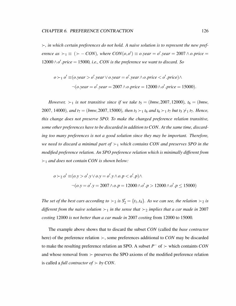
CHAPTER 6. PREFERENCE CONTRACTION 126
, in which certain preferences do not hold. A naive solution is to represent the new pref-
erence as 1 ≡ (−CON), where CON(o,o′) ≡ o.year = o′.year = 2007∧ o.price =
12000∧o′.price = 15000, i.e., CON is the preference we want to discard. So
o1 o′ ≡(o.year > o′.year∨o.year = o′.year∧o.price < o′.price)∧
¬(o.year = o′.year = 2007∧o.price = 12000∧o′.price = 15000).
However, 1 is not transitive since if we take t5 = (bmw,2007,12000), t6 = (bmw,
2007, 14000), and t7 = (bmw,2007,15000), then t5 1 t6 and t6 1 t7 but t5 61 t7. Hence,
this change does not preserve SPO. To make the changed preference relation transitive,
some other preferences have to be discarded in addition to CON. At the same time, discard-
ing too many preferences is not a good solution since they may be important. Therefore,
we need to discard a minimal part of 1 which contains CON and preserves SPO in the
modified preference relation. An SPO preference relation which is minimally different from
1 and does not contain CON is shown below:
o2 o′ ≡(o.y > o′.y∨o.y = o′.y∧o.p < o′.p)∧
¬(o.y = o′.y = 2007∧o.p = 12000∧o′.p > 12000∧o′.p≤ 15000)
The set of the best cars according to 2 is S′2 = t1, t4. As we can see, the relation 2 is
different from the naive solution 1 in the sense that 2 implies that a car made in 2007
costing 12000 is not better than a car made in 2007 costing from 12000 to 15000.
The example above shows that to discard the subset CON (called the base contractor
here) of the preference relation , some preferences additional to CON may be discarded
to make the resulting preference relation an SPO. A subset P− of which containts CON
and whose removal from preserves the SPO axioms of the modified preference relation
is called a full contractor of by CON.

CHAPTER 6. PREFERENCE CONTRACTION 127
6.2 Scenario of minimal preference contraction
In this section, we consider possible scenarios of user guided preference contraction. For
that, let us consider the notion of full contractor informally defined above. A full contractor
P− may be viewed as a union of the preferences CON to discard and a set of reasons of
discarding CON. Ideally, if a user decides to discard preferences, she also provides all the
reasons for such a change. In this case, the relation (−CON) is a consistent preference
relation (i.e., SPO). However, in real life scenarios, it is hard to expect that users always
provide complete information about the change they want to make. At the same time, the
number of alternative full contractors P− for a given and CON may be large or even
infinite for infinite preference relations. As a result, there is often a need to learn from the
user the reasons for discarding preferences. That may be done in a step-wise manner by
exploring possible alternatives and using user feedback to select the correct ones.
We envision the following scenario here. To find a complete set of preferences she
wants to discard, the user iteratively expresses the most obvious preferences CON that
should be dropped from her preference relation . After that, a possible set of reasons
P− for such a change is computed. To check if she is satisfied with the computed P−,
the impact of the performed change may be demonstrated to her (e.g., the result of the
winnow operator over a certain data set). If the full contractor P− does not represent the
change she actually wanted to make, the user may undo the change and select another
alternative or tune the contraction by elaborating it. One type of such elaboration can
be expressed as a set of additional preferences to discard. Another type of elaboration
which we propose here is preference protection. Because the exact reasons for contracting
CON are not known beforehand, some preferences which are important for the user may
be contracted in an intermediate P−. To avoid that, a user can impose a requirement of
protecting a set of preferences from removal. The corresponding contraction operator is
called here preference-protecting contraction. This iterative process stops when the user is

CHAPTER 6. PREFERENCE CONTRACTION 128
satisfied with the computed full contractor.
An important property of the scenario above is that the set of reasons P− which is
computed as a result of the iterative process above has to be as small as possible. That is,
preferences that the user does not want to discard and that are not needed to be removed
to preserve the consistency of the modified preference relation should remain. To preserve
the minimality of preference change, two approaches are possible.
In the first one, the full contractor computed in every step is minimal. The correspond-
ing contraction operator here is called minimal preference contraction. It is guaranteed that
the full contractor P− computed in the last iteration (i.e., when P− is satisfactory for the
user) is minimal. Note that since there could be many possible minimal full contractors
of a preference relation by a base contractor, any of them may be picked assuming that if
the user is not completely satisfied with it, she will tune the contraction in the next itera-
tion. In belief revision theory, the contraction operator with a similar semantics is called
maxichoice contraction [Han98].
In the other variant, the full contractor P− computed in every step is not necessary min-
imal. However, the user can make P− smaller by specifying the preferences which should
be protected from removal. The full contractor computed in the last step may be not mini-
mal, but sufficiently small to meet the user expectations. We propose to construct P− as the
union of all minimal full contractors of the preference relation by CON. This contraction
operator is called meet contraction if no preferences need to be preserved, and preference-
protecting meet contraction if preference preservation is required. Similar operators in
belief revision are full meet contraction, and partial meet contraction [Han98].
We note that the operations of preference contraction we propose in this chapter should
be understood in the context of the scenario discussed above. However, the practical details
of the scenario are beyond the scope of this work.

CHAPTER 6. PREFERENCE CONTRACTION 129
6.3 Preference contraction in binary relation framework
Here we formally define the operation of preference contraction in the binary relation
framework. We assume that when a user intends to discard some preferences, he or she
expresses the preferences to discard as a binary relation called a base contractor. The in-
terpretation of each pair in a base contractor is that the first tuple should not be preferred
to the second tuple. We require base contractor relations to be subsets of the preference re-
lation to be contracted. Hence, a base contractor is irreflexive but not necessary transitive.
Apart from that, we do not impose any other restrictions on the base contractors (e.g., they
can be finite of infinite), unless stated otherwise. Throughout the chapter, base contractors
are typically referred to as CON.
DEFINITION 6.1 A binary relation P− is a full contractor of a preference relation
by CON if CON ⊆ P− ⊆, and ( − P−) is a preference relation (i.e., an SPO). The
relation (− P−) is called the contracted relation.
A relation P− is a minimal full contractor of by CON if P− is a full contractor of
by CON, and there is no other full contractor P′ of by CON s.t. P′ ⊂ P−.
DEFINITION 6.2 A preference relation is minimally contracted if it is contracted by
a minimal full contractor. Contraction is an operation of constructing a full contractor.
Minimal contraction is an operation of constructing a minimal full contractor.
The notion of a minimal full contractor narrows the set of full contractors. However, as
we illustrate in Example 6.3, a minimal full contractor is generally not unique for the given
preference and base contractor relations. Moreover, the number of minimal full contractors
for infinite preference relations can be infinite. Thus, minimal contraction differs from
minimal preference revision [Cho07b] which is uniquely defined for given preference and
revising relations.
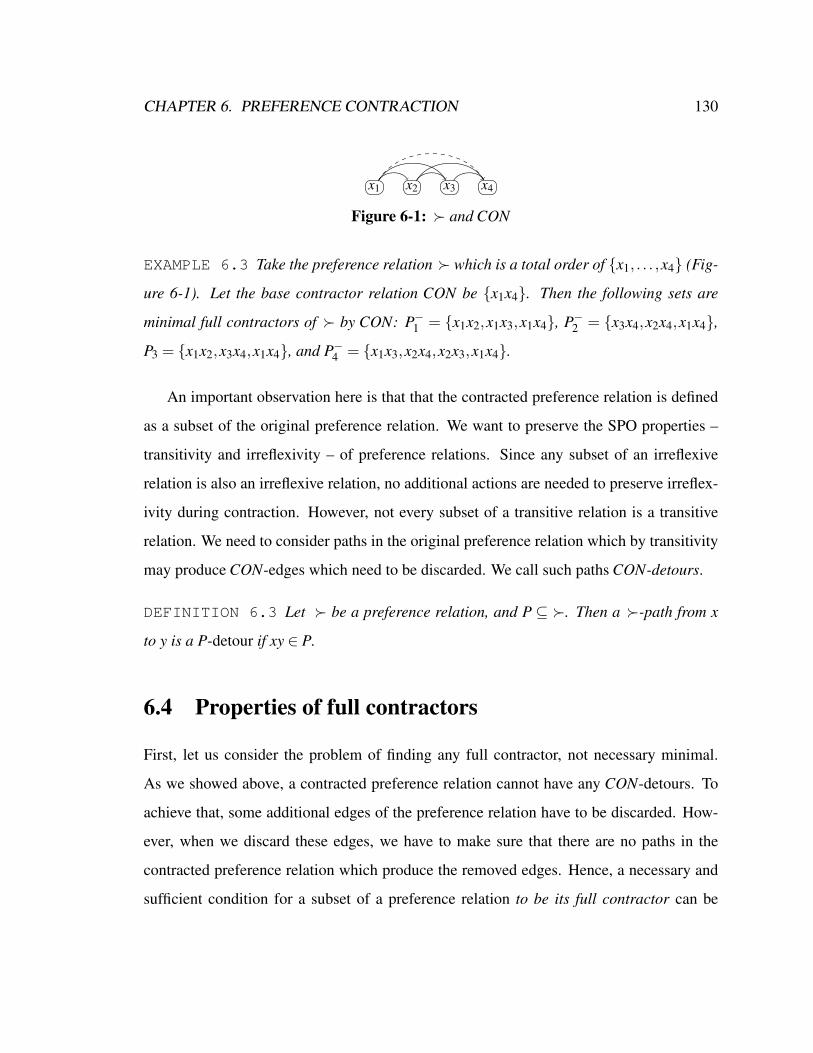
CHAPTER 6. PREFERENCE CONTRACTION 130
x1 x2 x3 x4
Figure 6-1: and CON
EXAMPLE 6.3 Take the preference relation which is a total order of x1, . . . ,x4 (Fig-
ure 6-1). Let the base contractor relation CON be x1x4. Then the following sets are
minimal full contractors of by CON: P−1 = x1x2,x1x3,x1x4, P−2 = x3x4,x2x4,x1x4,
P3 = x1x2,x3x4,x1x4, and P−4 = x1x3,x2x4,x2x3,x1x4.
An important observation here is that that the contracted preference relation is defined
as a subset of the original preference relation. We want to preserve the SPO properties –
transitivity and irreflexivity – of preference relations. Since any subset of an irreflexive
relation is also an irreflexive relation, no additional actions are needed to preserve irreflex-
ivity during contraction. However, not every subset of a transitive relation is a transitive
relation. We need to consider paths in the original preference relation which by transitivity
may produce CON-edges which need to be discarded. We call such paths CON-detours.
DEFINITION 6.3 Let be a preference relation, and P ⊆ . Then a -path from x
to y is a P-detour if xy ∈ P.
6.4 Properties of full contractors
First, let us consider the problem of finding any full contractor, not necessary minimal.
As we showed above, a contracted preference relation cannot have any CON-detours. To
achieve that, some additional edges of the preference relation have to be discarded. How-
ever, when we discard these edges, we have to make sure that there are no paths in the
contracted preference relation which produce the removed edges. Hence, a necessary and
sufficient condition for a subset of a preference relation to be its full contractor can be

CHAPTER 6. PREFERENCE CONTRACTION 131
formulated in an intuitive way.
LEMMA 6.1 Given a preference relation (i.e., an SPO) and a full contractor CON, a
relation P− ⊆ is a full contractor of by CON if and only if CON ⊆ P−, and for every
xy ∈ P−, (− P−) contains no paths from x to y.
PROOF
⇐ Prove that if for all xy ∈ P−, ( −P−) contains no paths from x to y, then ( −P−)
is an SPO. The irreflexivity of ( −P−) follows from the irreflexivity of . Assume
(−P−) is not transitive, i.e., there are xz,zy ∈ (−P−) but xy 6∈ (−P−). If xy ∈ P−
then the path xz,zy is not disconnected which contradicts the initial assumption. If xy 6∈ P−,
then the assumption of transitivity of is violated.
⇒ First, CON 6⊆ P− implies that P− is not a full contractor of by CON by definition.
Second, the existence of a path from x to y in (−P−) for xy ∈ P− implies that (−P−)
is not transitive, which violates the SPO properties.
Now let us consider the property of minimality of full contractors. Let P− be any
minimal full contractor of a preference relation by a base contractor CON. Pick any
edge xy of P−. An important question which arises here is why is xy a member of P−?
The answer is obvious if xy is also a member of CON: every CON-edge has to be removed
from the preference relation. However, what if xy is not a member of CON? To answer
this question, let us introduce the notion of the outer edge set of an edge belonging to a full
contractor relation.
DEFINITION 6.4 Let CON be a base contractor of a preference relation , and P− be
a full contractor of by CON. Let xy ∈ P−−CON, and
Φ0(xy) = xy, and
Φi(xy) = uivi ∈ P−|∃ui−1vi−1 ∈Φi−1(xy) . ui = ui−1∧ vi−1vi ∈ (−P−)∨
vi−1 = vi∧uiui−1 ∈ (−P−), for i > 0.

CHAPTER 6. PREFERENCE CONTRACTION 132
Then the outer edge set Φ(xy) for xy is defined as
Φ(xy) =∞⋃
i=0
Φi(xy).
u x y v z
Figure 6-2: Φ(xy) for Example 6.4.
Intuitively, the outer edge set Φ(xy) of an edge xy ∈ (P−−CON) contains all the edges
of a full contractor P− which should be removed from P− (i.e., added back to the preference
relation ) to preserve the full contractor property of the result, should xy be removed from
P− (i.e., added back to the preference relation). The reasoning here is as follows. When
for some i, Φi(xy) is removed from P−, then Φi+1(xy) has to be also removed from P−.
Otherwise, for every edge in Φi+1(xy), there is a two-edge path in one of whose edges is
in Φi(xy) while the other is not contracted. Hence, if the SPO properties of (−P−) need
to be preserved, removing xy from P− requires recursively removing the entire Φ(xy) from
P−.
The next example illustrates the inductive construction of an outer edge set. Some
properties of outer edge sets are shown in Lemma 6.2.
EXAMPLE 6.4 Let a preference relation be the set of all edges in Figure 6-2, and P−
be defined by the dashed edges. Let us construct Φ(xy) (assuming that xy is not an edge of
the base contractor CON).
• Φ0(xy) = xy;
• Φ1(xy) = xv,xz;

CHAPTER 6. PREFERENCE CONTRACTION 133
• Φ2(xy) = uv,uz;
Thus, Φ(xy) = xy,xv,xz,uv,uz.
LEMMA 6.2 Let P− be a full contractor of a preference relation by a base contractor
CON. Then for every xy ∈ (P−−CON), Φ(xy) has the following properties:
1. for all uv ∈Φ(xy), u x and y v;
2. for all uv ∈Φ(xy), ux,yv 6∈ P−;
3. if (Φ(xy)∩CON) = /0, then P′ = (P−−Φ(xy)) is a full contractor of by CON.
PROOF
First, we prove that Properties 1 and 2 hold. We do it by induction on the index of Φi(xy)
used to construct Φ(xy). For every uv∈Φ0(xy), Properties 1 and 2 hold by the construction
of Φ0. Now let Properties 1 and 2 hold for Φn(xy), i.e.,
∀unvn ∈Φn(xy)→ un x∧ y vn∧unx,yvn 6∈ P− (1)
Pick any un+1vn+1 ∈Φn+1(xy). By construction of Φn+1(xy), we have
∃unvn ∈Φi(xy) . un+1 = un∧ vn vn+1∧ vnvn+1 6∈ P−∨
un+1 un∧ vn = vn+1∧un+1un 6∈ P− (2)
Note that un+1 x and y vn+1 follows from (1), (2), and transitivity of . Similarly,
un+1x,yvn+1 6∈ P− is implied by (1), (2), and transitivity of (−P−). Hence, Properties 1
and 2 hold for ∪ni=0Φi(xy) for any n.
Now we prove Property 3: (−P′) is an SPO and CON ⊆ P′. The latter follows from
CON ⊆ P− and Φ(xy)∩CON = /0. Irreflexivity of ( −P′) follows from irreflexivity of
. Assume ( −P′) is not transitive, i.e., there are uv 6∈ ( −P′) and uz,zv ∈ ( −P′).
CHAPTER 6. PREFERENCE CONTRACTION 134
Transitivity of ( −P−) implies that at least one of uz,zv is in Φ(xy). However, Property
1 implies that exactly one of uz,zv is in Φ(xy) and the other one is not in Φ(xy) and thus
in ( −P−). However, uz ∈ Φ(xy) and zv ∈ ( −P−) imply uv ∈ Φ(xy), and thus uv ∈
(−(P−−Φ(xy))) = (−P′), i.e., we derive a contradiction. A similar contradiction is
derived in the case uz ∈ ( −P−) and zv ∈ Φ(xy). Therefore, ( −P′) is an SPO and P′
is a full contractor of by CON.
Out of the three properties shown in Lemma 6.2, the last one is the most important. It
says that if an edge xy of a full contractor is not needed to disconnect any CON-detours,
then that edge may be dropped from the full contractor along with its entire outer edge set.
A more general result which follows from Lemma 6.2 is formulated in the next theorem. It
represents a necessary and sufficient condition for a full contractor to be minimal.
THEOREM 6.1 (Full-contractor minimality test). Let P− be a full contractor of
by CON. Then P− is a minimal full contractor of by CON if and only if for every
xy ∈ P−, there is a CON-detour in in which xy is the only P−-edge.
PROOF
⇐ The proof in this direction is straightforward. Assume that for every edge of the full
contractor P− there exists at least one CON-detour in which only that edge is in P−. If P−
loses any its subset P containing that edge, then there will be a CON-detour in having
no edges in (P−− P), and thus (P−− P) is not a full contractor of by CON by Lemma
6.1. Hence, P− is a minimal full contractor.
⇒ Let P− be a minimal full contractor. For the sake of contradiction, assume for some
xy ∈ P−, 1) there is no CON-detour which xy belongs to, or 2) any CON-detour xy belongs
to has at least one more P−-edge. If 1) holds, then Φ(xy) has no edges in CON by construc-
tion. Thus, Lemma 6.2 implies that (P−−Φ(xy)) is a full contractor of by CON. Since

CHAPTER 6. PREFERENCE CONTRACTION 135
Φ(xy) is not empty, we get that P− is not a minimal full contractor which is a contradiction.
If 2) holds, then we use the same argument as above and show that Φ(xy)∩CON = /0. If
Φ(xy)∩CON is not empty (i.e., some uv ∈Φ(xy)∩CON), then by Lemma 6.2,
u x∧ x y∧ y v∧ux,yv 6∈ P−,
and thus there is a CON-detour going from u to v in which xy is the only P−-edge. This
contradicts the initial assumption.
Note that using the definition of minimal full contractor to check the minimality of a full
contractor P− requires checking the full contractor properties of all subsets of P−. In con-
trast, the minimality checking method shown in Theorem 6.1 requires checking properties
of distinct elements of P− with respect to its other members.
Sometimes a direct application of the minimality test from Theorem 6.1 is hard because
it does not give any bound on the length of CON-detours. Hence, it is not clear how it can be
represented as a finite formula. Fortunately, the transitivity of preference relations implies
that the minimality condition from Theorem 6.1 can be stated in terms of paths of length at
most three.
COROLLARY 6.1 A full contractor P− of by CON is minimal if and only if for every
edge xy ∈ P−, there is a CON-detour consisting of at most three edges among which only
xy is in P−.
PROOF
⇐ Trivial.
⇒ For every xy ∈ P−, pick any CON-detour T in which the only P−-edge is xy. If its
length is less or equal to three, then the corollary holds. Otherwise, x is not the start node
of T , or y is not the end node of T , or both. Let the start node u of T be different from

CHAPTER 6. PREFERENCE CONTRACTION 136
x. Since the only common edge of T and P− is xy, every edge in the path from u to x
is an element of ( −P−). Transitivity of ( −P−) implies ux ∈ ( −P−). Similarly,
yv ∈ (−P−) for the end node of T if y is different from v. Hence, there is a CON-detour
of length at most three in which xy is the only element of P−.
As a result, the following tests can be used to check the minimality of a full contractor
P−. In the finite case, P− is minimal if the following relational algebra expression results
in an empty set
P - [πP2.X,P2.Y((R1 - P1) ./R1.Y=P2.X
P2 ./P2.Y=R3.X
(R3 - P3) ./R1.X=C.X , R3.Y=C.Y
C) ∪
πP2.X,P2.Y(P2 ./P2.Y=R3.X
(R3 - P3) ./P2.X=C.X , R3.Y=C.Y
C) ∪
πP2.X,P2.Y((R1 - P1) ./R1.Y=P2.X
P2 ./R1.X=C.X , P2.Y=C.Y
C) ∪ C ],
for the tables R, C and P with columns X and Y, storing , CON, and P− correspondingly.
In the finitely representable case, P− is minimal if the following formula is valid
∀x,y (FP−(x,y)⇒ F(x,y)∧∃u,v . FCON(u,v)∧ (F(u,x)∨u = x)∧
(F(y,v)∨ y = v)∧¬FP−(u,x)∧¬FP−(y,v)).
Below we show examples of checking minimality of full contractors using Corollary
6.1. We note that when the relations are definable using ERO-formulas, checking mini-
mality of a full contractor can be done by performing quantifier elimination on the above
formula.
EXAMPLE 6.5 Let a preference relation be defined by the formula F(o,o′) ≡ o.d <
o′.d, where d is a Q -attribute. Let a base contractor CON of be defined by the formula
FCON(o,o′)≡ (1≤ o.d ≤ 2∧o′.d = 4)∨ (o.d = 0∧o′.d = 3)
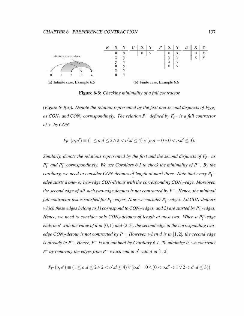
CHAPTER 6. PREFERENCE CONTRACTION 137
0 1 2 3 4
infinitely many edges
(a) Infinite case, Example 6.5
R X Yu xx yy vu yx vu v
C X Yu v
P X Yu xy vx vu v
D X Yu xx v
(b) Finite case, Example 6.6
Figure 6-3: Checking minimality of a full contractor
(Figure 6-3(a)). Denote the relation represented by the first and second disjuncts of FCON
as CON1 and CON2 correspondingly. The relation P− defined by FP− is a full contractor
of by CON
FP−(o,o′)≡ (1≤ o.d ≤ 2∧2 < o′.d ≤ 4)∨ (o.d = 0∧0 < o.d′ ≤ 3).
Similarly, denote the relations represented by the first and the second disjuncts of FP− as
P−1 and P−2 correspondingly. We use Corollary 6.1 to check the minimality of P−. By the
corollary, we need to consider CON-detours of length at most three. Note that every P−1 -
edge starts a one- or two-edge CON-detour with the corresponding CON1-edge. Moreover,
the second edge of all such two-edge detours is not contracted by P−. Hence, the minimal
full contractor test is satisfied for P−1 -edges. Now we consider P−2 -edges. All CON-detours
which these edges belong to 1) correspond to CON2-edges, and 2) are started by P−2 -edges.
Hence, we need to consider only CON2-detours of length at most two. When a P−2 -edge
ends in o′ with the value of d in (0,1) and (2,3], the second edge in the corresponding two-
edge CON2-detour is not contracted by P−. However, when d is in [1,2], the second edge
is already in P−. Hence, P− is not minimal by Corollary 6.1. To minimize it, we construct
P∗ by removing the edges from P− which end in o′ with d in [1,2]
FP∗(o,o′)≡ (1≤ o.d ≤ 2∧2 < o′.d ≤ 4)∨ (o.d = 0∧ (0 < o.d′ < 1∨2 < o′.d ≤ 3))

CHAPTER 6. PREFERENCE CONTRACTION 138
EXAMPLE 6.6 Take a preference represented by the table R, and a base contractor R
represented by the table C (Figure 6-3(b)). Consider the table P representing a base con-
tractor of R by C. Then the result of the relational algebra expression above evaluated for
these tables is shown in the table D. Since it is not empty, the full contractor represented
by P is not minimal. The minimality of P can be achieved by removing from it any (but only
one) tuple in D.
6.5 Construction of a minimal full contractor
In this section, we propose a method of computing a minimal full contractor. We use the
idea shown in Example 6.3. Pick for instance the set P−1 . That set was constructed as
follows: we took the CON-edge x1x4 and put in P−1 all the edges which start some path
from x1 to x4. For the preference relation from Example 6.3, P−1 turned out to be a
minimal full contractor. As is it shown in the next lemma, the set consisting of all edges
starting CON-detours is a full contractor by CON.
LEMMA 6.3 Let be a preference relation and CON be a base contractor relation of .
Then
P− := xy | ∃x′v ∈CON . x′ = x∧ x′ y∧ y v
is a full contractor of by CON.
PROOF
By construction of P−, CON ⊆ P−. Lemma 6.1 implies ( −P−) is an SPO. Hence,
(−P−) is a full contractor of by CON.
However, in the next example we show that such a full contractor is not always minimal.
Recall that by Theorem 6.1, for every edge of a full contractor there should be a CON-
detour which only shares that edge with the contractor. However, it may be the case that

CHAPTER 6. PREFERENCE CONTRACTION 139
an edge starting a CON-detour does not have to be discarded because the CON-detour is
already disconnected.
x1 x2 x3 x4 x5
(a) Preference relation
x1 x2 x3 x4 x5
(b) Preference relation (−P−)
x1 x2 x3 x4 x5
(c) Minimally contracted
Figure 6-4: Preference contraction
EXAMPLE 6.7 Let a preference relation be a total order of x1, . . . ,x5 (Figure 6-
4(a)). Let a base contractor CON be x1x4,x2x5. Let P− be defined as in Lemma 6.3.
That is P− = x1x2,x1x3,x1x4,x2x3,x2x4,x2x5. Then (−P−) is shown in Figure 6-4(b)
as the set of solid edges. P− is not minimal because (P−−x1x2) (Figure 6-4(c)) is also
a full contractor of by CON. In fact, (P−−x1x2) is a minimal full contractor of
by CON. As we can see, having the edge x1x2 in P− is not necessary. First, it is not a
CON-edge. Second, the edge x2x4 of the CON-detour x1 x2 x4 is already in P−.
As we have shown in Example 6.7, a minimal full contractor can be constructed by
including in it only the edges which start some CON-detour, if the detour is not already
disconnected. Thus, before adding such an edge to a full contractor, we need to know if an
edge not starting that detour is already in the full contractor. Here we propose the following
idea of computing a minimal full contractor. Instead of contracting by CON at once,
split CON into strata , and contract incrementally by the strata of CON. A stratum of
CON consists of only those edges whose detours can be disconnected simultaneously in a
minimal way. The method of splitting a full contractor into strata we propose to use is as
follows.

CHAPTER 6. PREFERENCE CONTRACTION 140
DEFINITION 6.5 The stratum index of an edge xy ∈CON is the maximum length of a
-path started by y and consisting of the end nodes of CON-edges. A stratum is the set of
all CON-edges with the same stratum index .
This method of stratification has the following useful property. If a preference relation
is contracted minimally by the strata with indices of up to n, then contracting that relation
minimally by the stratum with the index n+1 minimally guarantees the minimality of the
entire contraction.
Clearly, if a preference relation is infinite, a tuple can start -paths of arbitrarily large
lengths. Therefore, the stratum index of CON-edge may be undefined. We exclude such
cases here, so we can assume that for each edge of CON relations, the stratum index is
defined.
DEFINITION 6.6 Let CON be a base contractor of a preference relation . Let KCON =
y | ∃x . xy ∈ CON, and CON = ∩ KCON ×KCON . Then CON is stratifiable iff for
every y ∈ KCON there is an integer k such that all the paths started by y in CON are of
length at most k. CON is finitely stratifiable iff there is a constant k such that all paths in
CON are of length at most k.
Definition 6.6 implies that for every edge of stratifiable CON, the stratum index is de-
fined. Since the shortest path in CON is of length 0, the least stratum index for stratifiable
relations is 0. Below we present an approach of constructing a minimal full contractor for
a stratifiable relation CON.THEOREM 6.2 (Minimal full contractor construction). Let be a preference rela-
tion, and CON be a stratifiable base contractor of . Let Li be the set of the end nodes
of all CON-edges of stratum i. Then P−, defined as follows, is a minimal full contractor
of by CON
P− =∞⋃
i∈0
Ei,

CHAPTER 6. PREFERENCE CONTRACTION 141
where
Ei = xy | ∃v ∈ Li . xv ∈CON∧ x y∧ y v∧ yv 6∈ (P−i−1∪CON)
P−−1 = /0,
P−i =i⋃
j=0
Ei
Intuitively, the set Ei contains all the CON edges of stratum i along with the edges of
which need to be discarded to contract the preference relation by that stratum. P−i is the
union of all such sets up to stratum i.
PROOF OF THEOREM 6.2
Every Ei containts the CON-edges of stratum i. Thus, P− contains CON. Now we prove
that ( −P−) is an SPO. Its irreflexivity follows from the irreflexivity of . Transitivity
is proved by induction on stratum index.
It is given that is transitive. Now assume ( −P−n ) is transitive. Prove that (
−P−n+1) = (−P−n −En+1) is transitive. For the sake of contradiction, assume
∃x,y,z . xy 6∈ (−P−n+1)∧ xz,zy ∈ (−P−n+1) (1)
which implies
xz,zy 6∈ En+1∪P−n (2)
Transitivity of (−P−n ) and (1) imply xy ∈ (−P−n ) and thus xy ∈ En+1. Hence,
∃v ∈ Ln . xv ∈CON∧ x y∧ y v∧ yv 6∈ (P−n ∪CON) (3)
According to (3), y v. If y = v, then (2) and (3) imply xz ∈ En+1 which is a contradiction.

CHAPTER 6. PREFERENCE CONTRACTION 142
If y v, then xz 6∈ En+1 implies zv ∈ P−n ∪CON by the construction of En+1. Note that
zv ∈ CON implies zv is a CON-edge of stratum index n + 1 and thus either zy ∈ En+1
or yv ∈ P−n ∪CON, which contradicts (2) and (3). If zv ∈ P−n , then zy,yv 6∈ P−n implies
intransitivity of ( −P−n ), which contradicts the inductive assumption. Thus, P−n+1 is a
full contractor of by CON by induction. Now assume that ( −P−) is not transitive.
Violation of transitivity means that there is an edge xy ∈ P− such that there exists a path
from x to y none of whose edges is P− (Lemma 6.1). Since xy must be in P−n for some n, that
implies intransitivity of (−P−n ), which is a contradiction. Thus P− is a full contractor of
by CON.
Now we prove that P− is a minimal full contractor. If it is not, then by Theorem 6.1,
there is xy ∈ P− for which there is no CON-detour which shares with P− only the edge
xy. Note that xy ∈ P− implies xy ∈ En for some n. By definition of En, there is a CON-
detour x y v which shares with P−n only xy. Since all CON-detours which xy belongs
to have other P−-edges, yv ∈ P−. Since yv 6∈ P−n , there must exist k > n such that yv ∈ Ek.
However, that is impossible by construction: every CON-detour which may be started by
yv must have the stratum index not greater than n.
x1 x2 x3 x4 x5
(a) and CON
x1 x2 x3 x4 x5
(b) P−0
x1 x2 x3 x4 x5
(c) P−1
Figure 6-5: Using Theorem 6.2 to compute a minimal full contractor
EXAMPLE 6.8 Let a preference relation be a total order of x1, . . . ,x5 (Figure 6-5(a),
the transitive edges are omitted for clarity). Let a base contractor CON be x1x4,x2x5.
We use Theorem 6.2 to construct a minimal full contractor of by CON. The relation
CON has two strata: L0 = x2x5, L1 = x1x4. Then E0 = x2x3,x2x4,x2x5, P−0 = E0,
E1 = x1x3,x1x4, P−1 = E0∪E1, and a minimal full contractor of by CON is P− = P−1 .

CHAPTER 6. PREFERENCE CONTRACTION 143
It is easy to observe that the full contractor P− constructed in Theorem 6.2 has the
property that its every edge starts at least one CON-detour in which xy is the only P−-
edge. Full contractors which have this property are called prefix. Prefix full contractors
are minimal by Theorem 6.1. It turns out that a prefix full contractor is unique for a given
preference relation and a given base contractor.
PROPOSITION 6.1 Given a preference relation and a base contractor CON stratifi-
able, there exists a unique prefix full contractor P− of by CON.
PROOF
The existence of a prefix full contractor follows from Theorem 6.2. The fact that every
prefix full contractor is equal to P− constructed by Theorem 6.2 can be proved by induction
in CON stratum index. Namely, we show that for every n, P−n is contained in any prefix full
contractor of by CON. Clearly, the set E0 contracting by the 0th stratum of CON has
to be in any prefix full contractor. Assume every edge in P−n is in any prefix full contractor
of by CON. If an edge xy ∈ En+1−CON, then there is a CON-detour x y v in which
xy is the only P−-edge (i.e., yv 6∈ P−). Hence if xy is not in some prefix full contractor P′,
then yv has to be in P′ by Lemma 6.1. However, P−n ⊂ P′ is enough to disconnect every
CON-detour with the stratum index up to n, and yv can only start a CON-detour with the
stratum index up to n. Hence P′ is not a minimal full contractor and P− is a unique prefix
full contractor.
6.6 Contraction by finitely stratifiable relations
In this section, we consider practical issues of computing minimal full contractors. In par-
ticular, we show how the method of constructing a prefix full contractor we have proposed
in Theorem 6.2 can be adopted to various classes of preference and base contractor rela-
tions. Note that the definition of the minimal full contractor in Theorem 6.2 is recursive.
CHAPTER 6. PREFERENCE CONTRACTION 144
Namely, to find the edges we need to discard for contracting the preference relation by the
stratum n + 1 of CON, we need to know which edges to discard for contracting it by all
the previous strata. It means that for base contractor relations which are not finitely strat-
ifiable (i.e., CON has infinite number of strata), the corresponding computation will never
terminate.
Now assume that CON is a finitely stratifiable relation. First we note that any base
contractor of a finite preference relation is finitely stratifiable: all paths in such preference
relations are not longer than the size of the relation, and base contractors are required to
be subsets of the preference relations. At the same time, if CON is a base contractor of
an infinite preference relation, then the finite stratification property of CON does not imply
the finiteness of CON. In particular, it may be the case that the length of all paths in CON
is bounded, but the number of paths is infinite. This fact is illustrated in the next example.
EXAMPLE 6.9 Let a preference relation be defined as o o′ ≡ o.price < o′.price.
Let every tuple have two Q -attributes: price and year. Let also the base contractor rela-
tions CON1 and CON2 be defined as
CON1(o,o′)≡ o.price < 1∧ (o′.price = 2∨o′.price = 3),
CON2(o,o′)≡ o.price < 1∧o′.price≥ 2.
then
KCON1 ≡ o | o.price = 2∨o.price = 3
KCON2 ≡ o | o.price≥ 2

CHAPTER 6. PREFERENCE CONTRACTION 145
and
oCON1 o′ ≡ o.price = 2∧o′.price = 3
oCON2 o′ ≡ o.price≥ 2∧o′.price > 2∧o.price < o′.price
Then CON1 is finitely stratifiable since despite the fact that the number of edges in
CON1 and in CON1 is infinite (due to the infiniteness of the domain of year), the length of
the longest path in CON1 equals to 1. Such paths are started by tuples with the value of
price equal to 2 and ended by tuples with price equal to 3. At the same time, CON2 is not
finitely stratifiable since price is a Q -attribute and thus there is no constant bounding the
length of all paths in CON2 .
Below we consider the cases of finite and finitely representable finitely stratifiable base
contractors separately.
6.6.1 Computing prefix full contractor: finitely representable rela-
tions
Here we assume that the relations CON and are represented by finite ERO-formulas
FCON and F. We aim to construct a finite ERO-formula FP− which represents a prefix full
contractor of by CON. The function minContr(F, FCON) shown below exploits
the method of constructing prefix full contractors from Theorem 6.2 adopted to formula
representations of relations. All the intermediate variables used in the algorithm store for-
mulas. Hence, for example, any expression in the form ′′F(x,y) := . . .′′ means that the
formula-variable F is assigned the formula written in the right-hand side, which has two
free tuple variables x and y. The operator QE used in the algorithm computes a quantifier-
free formula equivalent to its argument formula. For ERO-formulas, the operator QE runs
in time polynomial in the size of its argument formula (if the number of attributes in A is

CHAPTER 6. PREFERENCE CONTRACTION 146
fixed), and exponential in the number of attributes in A .
To compute formulas representing different strata of CON, the function getStratum
is used. It takes three parameters: the formula FCON representing the relation CON , the
formula FKCON representing the set of the end nodes of CON-edges, and the stratum index
i. It returns a formula which represents the set of the end nodes of CON-edges of stratum
i , or undefined if the corresponding set is empty. That formula is computed according
to the definition of a stratum.
PROPOSITION 6.2 Let CON be a finitely stratifiable base contractor of a preference
relation . Then Algorithm 6.1 terminates and computes a prefix full contractor of by
CON.
Algorithm 6.1 minContr(F, FCON)1: i = 0
2: FP−−1(x,y) := f alse
3: FKCON (y) := QE(∃x . FCON(x,y))
4: FCON (x,y) := FCON(x,y)∧FKCON (x)∧FKCON (y)
5: FLi(y) := getStratum(FCON ,FKCON , i)
6: while FLi is defined do
7: FEi(x,y) := QE(∃v . FLi(v)∧FCON(x,v)∧F(x,y)∧
(y = v∨F(y,v)∧¬(FP−i−1(y,v)∨FCON(y,v))))
8: FP−i(x,y) := FP−i−1
(x,y)∨FEi(x,y)
9: i := i + 1;
10: FLi(y) := getStratum(FCON ,FKCON , i)
11: end while
12: return P−i

CHAPTER 6. PREFERENCE CONTRACTION 147
Algorithm 6.2 getStratum(FCON , FKCON , i)
Require: i≥ 0
1: if i = 0 then
2: FLi(y) := QE( FKCON (y)∧¬∃x1(FCON (y,x1)))
3: else
4: FLi(y) := QE( ∃x1, . . . ,xi . FCON (y,x1)∧FCON (x1,x2)∧ . . .∧FCON (xi−1,xi))∧
¬∃x1, . . . ,xi+1 . FCON (y,x1)∧FCON (x1,x2)∧ . . .∧FCON (xi,xi+1)))
5: end if
6: if ∃y . FLi(y) then
7: return FLi
8: else
9: return undefined
10: end if
Proposition 6.2 holds because Algorithm 6.1 uses the construction from Theorem 6.2.
Below we show an example of computing a prefix full contractor for a finitely representable
preference relation.
EXAMPLE 6.10 Let a preference relation be defined by the following formula
F(o,o′)≡ o.m = BMW ∧o′.m = VW ∨o.m = o′.m∧o.price < o′.price
and a base contractor CON be defined by
FCON(o,o′)≡ o.m = o′.m∧ ((11000≤ o.price≤ 13000∧o′.price = 15000)∨
(10000≤ o.price≤ 12000∧o′.price = 14000))
where m is a C -attribute and price is a Q -attribute. Then FKCON (o) ≡ o.price = 14000∨

CHAPTER 6. PREFERENCE CONTRACTION 148
o.price = 15000 and FCON (o,o′)≡ F(o,o′)∧FKCON (o)∧FKCON (o′). The end nodes of the
CON strata are defined by the following formulas:
FL0(o)≡o.price = 15000∧o.m 6= BMW
FL1(o)≡o.price = 15000∧o.m = BMW ∨o.price = 14000∧o.m 6= BMW
FL2(o)≡o.price = 14000∧o.m = BMW.
The relations contracting all CON strata are defined by the following formulas
FE0(o,o′)≡o.m = o′.m 6= BMW ∧11000≤ o.price≤ 13000∧13000 < o′.price≤ 15000
FE1(o,o′)≡o.m = o′.m = BMW ∧11000≤ o.price≤ 13000∧13000 < o′.price≤ 15000∨
o.m = o′.m 6= BMW ∧10000≤ o.price < 11000∧13000 < o′.price≤ 14000
FE2(o,o′)≡o.m = o′.m = BMW ∧10000≤ o.price≤ 11000∧13000 < o′.price≤ 14000
Finally, a full contractor P− of by CON is defined by
FP−(o,o′)≡ o.m = o′.m∧ (11000≤ o.price≤ 13000∧13000 < o′.price≤ 15000∨
10000≤ o.price < 11000∧13000 < o′.price≤ 14000)
We note that the finite stratification property of CON is crucial for the termination of
the algorithm: the algorithm does not terminate for not finitely stratifiable relations.
6.6.2 Computing prefix full contractor: finite relations
In this section, we consider finite relations and CON. We assume that the relations are
stored in separate tables: a preference relation table R and a base contractor table C, each
having two columns X and Y . Every tuple in a table corresponds to an element of the

CHAPTER 6. PREFERENCE CONTRACTION 149
corresponding binary relation. Hence, R has to be an SPO and C ⊆ R. Here we present
an algorithm of computing a prefix full contractor of a preference relation by CON
represented by such tables. Essentially, the algorithm is an adaptation of Theorem 6.2.
Algorithm 6.3 minContrFinite(R, C)Require: R is transitive, C ⊆ R
1: P←C
2: /* Get the end nodes of all C-edges */
3: EC← πY (C)
4: /* RC is related to R as CON to in Definition 6.6 */
5: RC← πR.X , R.Y (EC1 ./EC1.Y=R.X
R ./EC2.Y=R.Y
EC2)
6: while EC not empty do
7: /* Get the end nodes of the next stratum C-edges */
8: E ← EC − πX (RC)
9: /* Prepare EC and RC for the next iteration */
10: EC← EC − E
11: RC← RC − RC ./RC.Y=E.Y
E
12: /* Add to P the R-edges contracting the current stratum of C*/
13: P← P ∪ πR1.X , R1.Y (R1 ./R1.Y = R2.X
(R2 − P) ./R1.X = C.X , R2.Y = C.Y
(C ./C.Y = E.Y
E))
14: end while
15: return P
The function minContrFinite takes two arguments: a table R and a table C. The
function is implemented in terms of relational algebra operators. First, it constructs two
tables: EC storing the end nodes of all C-edges, and RC storing a restriction of the original
preference relation R to EC. These two tables are needed for obtaining the strata of C.
After that, the function picks all strata of C one by one and contracts the original preference
relation by each stratum in turn, as shown in Theorem 6.2.
CHAPTER 6. PREFERENCE CONTRACTION 150
The extraction of the strata of CON in the order of the stratum index is performed as
follows. It is clear that the nodes ending CON-edges of stratum 0 do not start any edge in
RC. The set E computed in line 8 is a difference of the set EC of the nodes ending C-edges
and the nodes starting some edges in RC. Hence, E stores all the nodes ending C-edges
of stratum 0. To get the end nodes of the next stratum of C, we need remove all the edges
from RC which end in members of E, and remove E from EC. After the stratum with the
highest index is obtained, the relation EC becomes empty.
PROPOSITION 6.3 Algorithm 6.3 computes a prefix full contractor of R by C. Its run-
ning time is O(|C|2 · |R| · log|R|).
Proposition 6.3 holds because Algorithm 6.3 uses the construction from Theorem 6.2.
The stated running time may be obtained by applying some simple optimizations: (i) sort-
ing EC after constructing it (line 3), (ii) sorting on X , Y the table R and the table RC right
after its construction (line 5), (iii) keeping these relations sorted after every change. In
addition to that, we store the relation P containing the intermediate full contractor edges as
a copy of R, in which the edges which belong to the prefix full contractor are marked. By
doing so, P is maintained in the sorted state throughout the algorithm.
6.7 Preference-protecting contraction
Consider the operation of minimal preference contraction described above. In order to
contract a preference relation, a user has to specify a base contractor CON. The main
criteria we use to define a contracted preference relation is minimality of preference change.
However, a minimal full contractor P− may contain additional preferences which are not in
CON. So far, we have not paid attention to the contents of P−, assuming that any minimal
full contractor is equally good for a user. However, this may not be the case in real life.
Assume that an original preference relation is combined from two preference relations

CHAPTER 6. PREFERENCE CONTRACTION 151
= old ∪ recent , where old describes user preferences introduced by the user a long
time ago, and recent describes more recent preferences. Now assume that the user wants to
contract by CON, at least two minimal full contractors are possible: P−1 which consists
of CON and some preferences of old , and P−2 consisting of CON and some preferences
of recent . Since recent has been introduced recently, discarding members of old may
be more reasonable then members of recent . Hence, sometimes there is a need to compute
full contractors which protect some existing preferences from removal.
Here we propose an operator of preference-protecting contraction. In addition to a
base contractor CON, a subset P+ of the original preference relation to be protected from
removal in the contracted preference relation may also be specified. Such a relation is com-
plementary with respect to the base contractor: the relation CON defines the preferences to
discard, whereas the relation P+ defines the preferences to protect.
DEFINITION 6.7 Let be a preference relation and CON be a base contractor of
. Let a relation P+ be such that P+ ⊆. A full contractor P− of by CON such
that P+∩P− = /0 is called a P+-protecting full contractor of by CON. A minimal full
contractor P− of by CON such that P+∩P− = /0 is called a P+-protecting minimal full
contractor of by CON.
Given any full contractor P− of by CON, by Lemma 6.1, P− must contain at least
one edge from every CON-detour. Thus, if P+ contains an entire CON-detour, protecting
P+ while contracting by CON is not possible.
THEOREM 6.3 Let CON be a stratifiable base contractor relation of a preference re-
lation such that P+ ⊂. There exists a minimal full contractor of by CON that
protects P+ if and only if TC(P+) ∩CON = /0.
As we noted, the necessary condition of the theorem above follows from Lemma 6.1.
The sufficient condition follows from Theorem 6.4 we prove further.
CHAPTER 6. PREFERENCE CONTRACTION 152
A naive way of computing a preference-protecting minimal full contractor is by finding
a minimal full contractor P− of (− P+) and then adding P+ to P−. However, (− P+)
is not an SPO in general, thus obtaining SPO of − (P−∪P+) becomes problematic.
The solution we propose here uses the following idea. First, we find a base contractor
CON′ such that minimal contraction of by CON′ is equivalent to minimal contraction of
by CON with protected P+. After that, we compute a minimal full contractor of by
CON′ using Theorem 6.2.
Recall that minimal full contractors constructed in Theorem 6.2 are prefix, i.e., every
edge xy in such a full contractor starts some CON-detour in which xy is the only edge of
the contractor. Thus, if no member of P+ starts a CON-detour in , then the minimal full
contractor and P+ have no common edges. Otherwise assume that an edge xy ∈ P+ starts a
CON-detour in . By Lemma 6.1, any P+-protecting full contractor P− has to contain an
edge different from xy which belongs to CON-detours started by xy. Moreover, for CON-
detours of length two started by xy, P− has to contain the edges ending those CON-detours.
Such a set of edges is defined as follows:
Q = xy | ∃u : u x y∧uy ∈CON∧ux ∈ P+.
It turns out that the set Q is not only contained in any P+-protecting full contractor,
but it can also be used to construct a P+-protecting minimal full contractor as shown in the
next theorem.
THEOREM 6.4 Let be a preference relation, and CON be a stratifiable base con-
tractor of . Let also P+ be a transitive relation such that P+ ⊆ and P+∩CON = /0.
Then the prefix full contractor of by CON ∪Q is a P+-protecting minimal full con-
tractor of by CON.

CHAPTER 6. PREFERENCE CONTRACTION 153
PROOF
Let P− be a prefix full contractor of by CON′ = CON ∪Q. We prove that P−∩P+ = /0,
i.e., P− protects P+. For the sake of contradiction, assume there is xy ∈ P+∩P−. We show
that this contradicts the prefix property of P−. Since P− is a prefix full contractor, there is
a CON′-detour from x to some v in , started by xy and having only the edge xy in P−. We
have two choices: either it is a CON-detour or a Q-detour. Consider the first case. Clearly,
y 6= v, otherwise P+∩CON 6= /0. Thus, xv ∈CON and x y v (Figure 6-6(a)). yv ∈ Q
follows from xy ∈ P+, xv ∈CON and the construction of Q. Note that every path from y to
v in contains a P−-edge because P− is a full contractor of by CON∪Q. That implies
that no CON-detour from x to v started by xy has only xy in P− which contradicts the initial
assumption.
Consider the second case, i.e., there is a Q-detour from x to some v started by xy and
having only the edge xy in P−. Since xv ∈ Q, there is uv ∈CON such that ux ∈ P+ (Figure
6-6(b)). ux,xy ∈ P+ imply uy ∈ P+ by transitivity of P+. uy ∈ P+ and uv ∈ CON imply
yv ∈ Q. That along with the fact that P− is a full contractor of by CON ∪Q implies that
every path in from y to v contains a P−-edge. Hence, there is no Q-detour from x to v
started by xy and having only xy in P−. That contradicts the initial assumption about xy.
Now we prove that P− is a minimal full contractor of by CON. The fact that it is
a full contractor of by CON follows from the fact that it is a full contractor of by a
superset CON′ of CON. We prove now its minimality. Since P− is a prefix full contractor of
by CON′, for every xy∈ P−, there is xv∈CON′ such that there is a corresponding detour
T in which xy is the only P−-edge. If it is a CON-detour, then xy satisfies the minimality
condition from Theorem 6.1. If it is a Q-detour, then there is a CON-edge uv such that
ux ∈ P+. We showed above that P− protects P+. Hence, the CON-detour obtained by
joining the edge ux and T has only xy in P−. Therefore, P− is a minimal full contractor of
by CON.

CHAPTER 6. PREFERENCE CONTRACTION 154
x y vP+ Q
CON
(a) P+-protection: case 1
u x y vP+ P+ Q
P+ Q
CON
(b) P+-protection: case 2
Figure 6-6: Proof of Theorem 6.4
Note that the sets of the end nodes of (CON ∪Q)-edges and the end nodes of CON-
edges coincide by the construction of Q. Therefore, (CON ∪Q) is stratifiable or finitely
stratifiable if and only if CON is stratifiable or finitely stratifiable, correspondingly. Hence,
if CON is a finitely stratifiable relation with respect to , Algorithms 6.1 and 6.3 can be
used to compute a preference-protecting minimal full contractor of by CON. If the re-
lations and CON are finite, then Q can be constructed in polynomial time in the size of
and CON by a relational algebra expression constructed from its definition. If the rela-
tions are finitely representable, then Q may be computed using the quantifier elimination
operator QE.
For Theorem 6.4 to apply, the relation P+ has to be transitive. Non-transitivity of P+
implies that there are two edges xy,yz ∈ P+ which should be protected while transitive
edge xz is not critical. However, a relation obtained as a result of preference-protecting
contraction is a preference relation (i.e., SPO). Hence, the edge xz will also be protected in
the resulting preference relation. This fact implies that protecting any relation is equivalent
to protecting its minimal transitive extension: its transitive closure. Therefore, if P+ is
not transitive, one needs to compute its transitive closure to use Theorem 6.4. For finite
relations, transitive closure can be computed in polynomial time [CLRS01]. For finitely
representable relations, Constraint Datalog [KKR95] can be used to compute transitive
closure.
Another important observation here is that the P+-protecting minimal full contractor of
by CON computed according to Theorem 6.4 is not necessary a prefix full contractor of

CHAPTER 6. PREFERENCE CONTRACTION 155
x1 x2 x3 x4 x5
(a) , CON, and P+
x1 x2 x3 x4 x5
(b) and CON′
x1 x2 x3 x4 x5
(c) P−0
x1 x2 x3 x4 x5
(d) P−1
Figure 6-7: Using Theorem 6.4 to compute a preference-protecting minimal full contractor
by CON. This fact is illustrated in the following example.
EXAMPLE 6.11 Let a preference relation be a total order of x1, . . . ,x5 (Figure 6-
7(a), the transitive edges are omitted for clarity). Let a base contractor CON be x1x4,x2x5,
and P+ = x1x3,x2x3,x4x5.
The existence of a minimal P+-protecting full contractor of by CON follows from
Theorem 6.3. We use Theorem 6.4 to construct it. The set Q is equal to x3x4,x3x5
and CON′ = x1x4,x2x5,x3x4,x3x5. We construct a prefix full contractor of by CON′.
The relation CON′ has two strata: L0 = x2x5,x3x5, L1 = x1x4,x3x4. Then E0 =
x2x5,x3x5,x2x4,x3x4, P−0 = E0, E1 = x1x4,x3x4, P−1 = E0 ∪ E1, and P− = P−1 . By
Theorem 6.4, P− is a P+-protecting minimal full contractor of by CON. However, P−
is not a prefix full contractor of by CON, because the edges x3x4, x3x5 do not start any
CON-detour.
6.8 Meet preference contraction
In this section, we consider the operation of meet preference contraction. In contrast to the
preceding sections, where the main focus was the minimality of preference relation change,
the contraction operation considered here changes a preference relation not necessarily in
a minimal way. A full meet contractor of a preference relation is semantically a union
of all minimal sets of reasons of discarding a given set preferences. When a certain set of
preferences is required to be protected while contracting a preference relation, the operation

CHAPTER 6. PREFERENCE CONTRACTION 156
u x y v
(a) and CON1
u x y v
(b) and CON2
Figure 6-8: Example 6.12
of preference-protecting meet contraction may be used.
DEFINITION 6.8 Let be a preference relation, CON a base contractor of , and
P+ ⊆. The relation Pm is a full meet contractor of by CON iff
Pm =⋃
P−∈P m
P−,
for the set P m of all minimal full contractors of of CON. The relation PmP+ is a full
P+-protecting meet contractor of by CON iff
PmP+ =
⋃P−∈P m
P+
P−,
for the set P mP+ of all P+-protecting minimal full contractors of of CON.
Note that the relations (−Pm) and (−PmP+) can be represented as intersections of
preference (i.e., SPO) relations and thus are also preference (i.e., SPO) relations. Let us
first consider the problem of constructing full meet contractors.
By the definition above, an edge xy is in the full meet contractor of a preference relation
by CON if there is a minimal full contractor of by CON which contains xy. Theorem
6.1 implies that if there is no CON-detour in containing xy, then xy is not in the corre-
sponding full meet contractor. However, the fact that xy belongs to a CON-detour is not a
sufficient condition for xy to be in the corresponding full meet contractor.
EXAMPLE 6.12 Let a preference relation be a total order of u,x,y,v. Let also
CON1 = uv (Figure 6-8(a)) and CON2 = uv,yv (Figure 6-8(b)). There is only one

CHAPTER 6. PREFERENCE CONTRACTION 157
CON1- and CON2-detour containing xy: u x y v. There is also a minimal full contrac-
tor of by CON1 which contains xy: P−1 = uy,xv,xy,uv. However, there is no minimal
full contractor of by CON2 which contains xy because the edge yv of the CON2-detour
u x y v is in CON2.
In Theorem 6.5, we show how full meet contractors can be constructed in the case of
finitely stratifiable base contractors . According to that theorem, a -edge xy is in the full
meet contractor of by CON if and only if there is a full contractor P− of by CON such
that xy is the only P−-edge in some CON-detour. We use Theorem 6.3 to show that there
is a minimal full contractor of by CON which contains xy while the other edges of the
detour are protected.
THEOREM 6.5 Let CON be a finitely stratifiable base contractor of a preference rela-
tion . Then the full meet contractor of by CON is
Pm = xy | ∃uv ∈CON . u x y v∧
(ux ∈ (−CON)∨u = x)∧ (yv ∈ (−CON)∨ y = v)
PROOF
By Corollary 6.1, an edge xy is in a minimal full contractor P− of by CON, if there
is CON-detour of at most three edges in in which xy is the only P−-edge. Hence any
minimal full contractor is a subset of Pm. Now take every edge xy of Pm and show there is a
minimal full contractor of by CON which contains xy. Let u x y v for uv ∈CON.
Let us construct a set P′ as follows:
P′ =
ux,yv if u x∧ y v
ux if u x∧ y = v
yv if u = x∧ y v
/0 if u = x∧ y = v

CHAPTER 6. PREFERENCE CONTRACTION 158
u x y v
Figure 6-9: , CON, and P+ from Example 6.13
P′ is transitive, P′∩CON = /0, and P′⊆. Theorem 6.3 implies that there is a P′-protecting
minimal full contractor P− of by CON. Since P− protects P′, there is a CON-detour in
from u to v in which xy is the only P−-edge. This implies that xy ∈ P−.
Now consider the case of P+-protecting full meet contractors. A naive solution is to
construct it as the difference of Pm defined above and P+. However, in the next example
we show that such solution does not work in general.
EXAMPLE 6.13 Let a preference relation be a total order of u,x,y,v (Figure 6-9).
Let also CON = uy,xv and P+ = ux. Note that yv 6∈ P+, and by Theorem 6.5, yv ∈ Pm.
Hence, yv ∈ (Pm−P+). However, note that ux ∈ P+ implies that xy must be a member
of every P+-protecting full contractor in order to disconnect the path from u to y. Hence,
there is no CON-detour in which yv is the only edge of the full contractor, and yv is not a
member of any P+-protecting full contractor.
The next theorem shows how a P+-protecting full contractor may be constructed. The
idea is similar to Theorem 6.5. However, to construct a full meet contractor, we used the
set CON as a common part of all minimal full contractors. In the case of P+-protecting full
meet contractor, a superset CP+ of CON is contained in all of them. Such a set CP+ may be
viewed as a union of CON and the set of all edges of that must be discarded due to the
protection of P+.
THEOREM 6.6 Let CON be a finitely stratifiable base contractor of a preference re-
lation , and P+ a transitive relation such that P+ ⊆ and P+∩CON = /0. Then the

CHAPTER 6. PREFERENCE CONTRACTION 159
P+-protecting full meet contractor of by CON is
PmP+ = xy | xy 6∈ P+∧∃uv ∈CON . u x y v ∧
(ux ∈ (−CP+)∨u = x)∧ (yv ∈ (−CP+)∨ y = v),
for
CP+ = xy | ∃uv ∈CON . u x y v∧ (ux ∈ P+∨u = x)
∧ (yv ∈ P+∨ y = v)
PROOF
First, it is easy to observe that CP+ is a subset of any P+-protecting full contractor of
by CON. It is constructed from the edges xy which participate in CON-detours of length at
most three where all the other edges have to be protected. Since every CON-detour has to
have at least one edge in a full contractor, xy has to be a member of every full contractor.
We show that every P+-protecting minimal full contractor P− of by CON is a subset
of PmP+ . If some xy ∈ P−, then by Corollary 6.1 there is an edge uv ∈ CON such that
u x y v and ux,yv 6∈ P−. We show that xy ∈ PmP+ . That holds if xy 6∈ P+ (which holds
for P− by definition) and
(ux ∈ (−CP+)∨u = x)∧ (yv ∈ (−CP+)∨ y = v)
If both u = x and y = v hold then the expression above holds. Now assume u x (the case
y v is similar). If ux ∈CP+ then, as we showed above, ux ∈ P− which is a contradiction.
Hence, ux ∈ (−CP+) and xy ∈ PmP+ . Finally, P− ⊆ Pm
P+ .
Now we show that every xy ∈ PmP+ is contained in every P+-protecting minimal full
contractor of by CON. The proof is similar to the proof of Theorem 6.5. By definition of

CHAPTER 6. PREFERENCE CONTRACTION 160
PmP+ , take xy such that u x y v. Construct the set P′ for xy as in the proof of Theorem
6.5. We show that for the set P′′ = TC(P+∪P′) we have P′′∩CON = /0. For the sake of
contradiction, assume P′′∩CON 6= /0. This implies that there is a CON-detour consisting of
P+ and P′ edges. Having only P+-edges in the detour contradicts the initial assumption that
P+∩CON = /0. Having a single edge of P′ in the detour implies that the edge (either ux or
yv) is in CP+ , which contradicts the definition of PmP+ . Having both ux and yv in the detour
implies that xy ∈ P+ which also contradicts the definition of PmP+ . Hence, P′′∩CON = /0,
and by Theorem 6.4, there is a P′′-protecting minimal full contractor P− of by CON
which is also a P+-protecting minimal full contractor. Since there is a CON-detour in
which xy is unprotected by P−, xy ∈ P−.
We note that given the expressions for the meet and P+-protecting full meet contrac-
tors in Theorems 6.5 and 6.6, one can easily obtain such contractors for finite and finitely
representable relations: by evaluation of a relational algebra query in the former case and
by quantifier elimination in the latter case.
x1 x2 x3 x4 x5
(a) and CON
x1 x2 x3 x4 x5
(b) −Pm
x1 x2 x3 x4 x5
(c) , CON, and P+
x1 x2 x3 x4 x5
(d) −PmP+
Figure 6-10: Computing full meet contractor and P+-protecting full meet contractor
EXAMPLE 6.14 Let a preference relation be a total order of x1, . . . ,x5 (Figure 6-
10(a), the transitive edges are omitted for clarity). Let a base contractor CON be x1x3,
x2x3, x2x5, and P+ = x2x4.
A full meet contractor Pm of by CON is x1x3,x2x3,x2x5,x2x4,x3x4,x4x5. The result-
ing contracted preference relation is shown on Figure 6-10(b). A P+-protecting full meet
contractor of by CON is x1x3,x2x3,x2x5,x4x5. The resulting contracted preference
relation is shown on Figure 6-10(d). Note that CP+ here is CON∪x4x5.

CHAPTER 6. PREFERENCE CONTRACTION 161
6.9 Querying with contracted preferences
In this section, we show some new techniques which can be used to optimize the evaluation
of the winnow operator under contracted preferences.
In user-guided preference modification frameworks [Cho07b, BGS06], it is assumed
that users alter their preferences after examining sets of the most preferred tuples returned
by winnow. Thus, if preference contraction is incorporated into such frameworks, there is
a need to compute winnow under contracted preference relations. Here we show how the
evaluation of winnow can be optimized in such cases.
Let be a preference relation, CON be a base contractor of , P− be a full contractor
of by CON, and the contracted preference relation ′= ( −P−). Denote the set of
the starting and the ending tuples of R-edges for a binary relation R as S(R) and E(R)
correspondingly.
S(R) = x | ∃y . xy ∈ R
E(R) = y | ∃x . xy ∈ R
Let us also define the set M(CON) of the tuples which participate in CON-detours in
M(CON) = y | ∃x,z . x y∧ xz ∈CON∧ y z
Assume we also know quantifier-free formulas FS(P−), FE(P−), FM(CON), and FS(CON) repre-
senting these sets for P− and CON. Then the following holds.
PROPOSITION 6.4 Given a finite set of tuples r
1. w(r)⊆ w′(r)
2. If σFS(P−)(w(r)) = /0, then w(r) = w′(r).

CHAPTER 6. PREFERENCE CONTRACTION 162
3. If P− is a prefix full contractor, then σFS(P−)(r) = σFS(CON)(r)
4. w′(r) = w′(w(r)∪σFE(P−)(r))
PROOF
1. By definition, w(r) contains the set of undominated tuples w.r.t the preference re-
lation . Thus, ′⊂ implies that if a tuple o was undominated w.r.t , it will be
undominated w.r.t ′, too. Hence, w(r)⊆ w′(r).
2. the SPO of implies that for every tuple o not in w(r), there is a tuple o′ ∈ w(r)
such that o′ o. Hence, if no edges going from w(r) are contracted by P−, every
o 6∈ w(r) will still be dominated according to ′.
3. Follows from the definition of the prefix contraction.
4. From 1 we know that w(r) ⊆ w′(r). For every tuple o ∈ w′(r)−w(r), at least
one edge going to it in has been contracted by P−. Thus, w′(r) ⊆ w(r)∪
σFE(P−)(r) and w′(r) = w′(w(r)∪σFE(P−)
(r)).
According to Proposition 6.4, the result of winnow under a contracted preference is al-
ways a superset of the result of winnow under the original preference. The second property
shows when the contraction does not change the result of winnow. Running the winnow
query is generally expensive, thus one can first evaluate σFS(P−)(or σFS(CON) , if P− is a prefix
contraction) over the computed result of the original winnow. If the result is empty, then
computing the winnow under the contracted preference relation is not needed.
The last statement of the proposition is useful when the set r is large and thus running
w′ over the entire set r is expensive. Instead, one can compute σFE(P−)(r) and then evaluate
w′ over (w(r)∪σFE(P−)(r)) (assuming that w(r) is already known).

CHAPTER 6. PREFERENCE CONTRACTION 163
EXAMPLE 6.15 Let a preference relation be defined by F(o,o′)≡ o.p < o′.p, and a
base contractor CON of be defined by FCON(o,o′) ≡ o.p = 0∧ o′.p = 3, where p is an
Q -attribute. Take set of tuples r = 1,2,3,4 in which every tuple has a single attribute p.
Then w(r) = 1. Take two minimal full contractors P−1 and P−2 of by CON defined by
the following formulas
FP−1(o,o′)≡ o.p = 0∧0 < o′.p≤ 3
FP−2(o,o′)≡ 0≤ o.p < 3∧o′.p = 3
The corresponding contracted preference relations 1 and 2 are defined by F1(o,o′)≡
F(o,o′) ∧¬FP−1(o,o′) and F2(o,o′) ≡ F(o,o′)∧¬FP−2
(o,o′). The full contractor P−1
is prefix, thus FS(P−1 )(o) ≡ FS(CON) ≡ o.p = 0. The full contractor P−2 is not prefix, and
FS(P−2 )(o)≡ 0≤ o.p < 3.
First, σFS(P−1 )(w(r)) = /0 implies w1(r) = w(r). Second, σFS(P−2 )
(w(r)) is not empty
and equal to 1. Note that FE(P−2 )(o) ≡ o.p = 3. Hence, σFE(P−2 )(r) = 3 and w2(r) =
w2(w(r)∪σFE(P−2 )(r)) = 1,3.
6.10 Experimental evaluation
In this section, we present the results of an experimental evaluation of the preference con-
traction framework proposed here. We implemented the following operators of preference
contraction: prefix contraction (denoted as PREFIX), preference-protecting minimal con-
traction (P+-MIN), meet contraction (MEET), and preference-protecting meet contraction
(P+-MEET). PREFIX was implemented using Algorithm 6.3, P+-MIN according to The-
orem 6.4, MEET according to Theorem 6.5, and P+-MEET according to Theorem 6.6.
We used these operators to contract finite preference relations stored in a database table
R(X ,Y ). The preference relations used in the experiments were finite skyline preference

CHAPTER 6. PREFERENCE CONTRACTION 164
relations [BKS01]. Such relations are often used in database applications. We note that
such relations are generally not materialized (as database tables) when querying databases
with skylines. However, they may be materialized in scenarios of preference elicitation
[BGL07]. To generate such relations, we used the NHL 2008 Player Stats dataset [nhl08]
of 852 tuples. Each tuple has 18 different attributes out of which we used 5. All algorithms
used in the experiments were implemented in Java 6. We ran the experiments on Intel
Core 2 Duo CPU 2.1 GHz with 2.0 GB RAM. All tables were stored in a PostgreSQL 8.3
database.
We have carried out two sets of experiments with the preference contraction algorithms.
In the first set, we model the scenario when base contractors are manually constructed by
user. Thus, we assume that such base contractors are of comparatively small size. In the
second set of experiments, we assume that base contractors are constructed automatically
and hence may be of large size.
Base contractors of small size
The aim of the experiments shown here is twofold. First, they demonstrate that the algo-
rithms of preference contraction we have proposed are of high performance and scale well
with the size of contracted preference relations (given base contractors of small size). Sec-
ond, they show that when a base contractor is of small size, the difference between the sizes
of full contractors computed by different algorithms may be significant. It implies that in
real life applications, an appropriate contraction algorithm needs to be selected carefully
depending on the required semantics.
Preference relations we use here consist of 2000, 3000, and 5000 edges. The sizes of
base contractors range from 1 to 35 edges. We do not pick more than 35 edges assuming
that in this scenario a user unlikely provides a large set of preferences to discard. For every
base contractor size, we randomly generated 10 different base contractors and computed the

CHAPTER 6. PREFERENCE CONTRACTION 165
average time spent to compute full contractors and the average size of them. The relations
P+ storing preferences to protect contained 25% of edges of the corresponding preference
relation.
Figure 6-11 shows how the running times of contraction operators depend on the size of
a preference relation to contract and the size of a base contractor. As we can observe, PRE-
FIX has the best performance among all operators, regardless of the size of the preference
relation and the base contractor relation. Note also that the running times of preference-
protecting operators are significantly larger then the running times of their unconstrained
counterparts. These running times predominantly depend on the time spent to compute the
transitive closure of P+.
0 10 20 30
100
101
102
103
|CON|
runn
ing
time
(ms)
PREFIXP+-MINMEET
P+-MEET
(a) | |= 2000
0 10 20 30100
101
102
103
|CON|
runn
ing
time
(ms)
PREFIXP+-MINMEET
P+-MEET
(b) | |= 3000
0 10 20 30
101
102
103
|CON|
runn
ing
time
(ms)
PREFIXP+-MINMEET
P+-MEET
(c) | |= 5000
Figure 6-11: Contraction performance. Small base contractors
Figure 6-12 shows the dependency of the full contractor size on the size of preference
relation and the size of base contractor. For every value of the base contractor size, the
charts show the average size of the corresponding full contractor. Notice that the prefer-
ence protection constraint does not affect much the sizes of full contractors computed by
PREFIX and P+-MIN – they almost always coincide. That is due to the fact that even
though the full contractors computed by these algorithms have different properties, they

CHAPTER 6. PREFERENCE CONTRACTION 166
are both minimal. At the same time, the sizes of full contractors computed by MEET and
P+-MEET differ significantly – the size of a full meet contractor is generally twice as large
as the size of the corresponding full P+-protecting meet contractor. This is justified by the
semantics of those full contractors: a full meet contractor is a union of all minimal full
contractors of by CON, while a full P+-protecting meet contractor is its subset.
Another important observation is that the sizes of minimal full contractors (PREFIX and
P+-MIN) and full meet contractors (MEET and P+-MEET) differ significantly. Hence,
the constraint of minimality has a high effect on the sizes of full contractors when base
contractors are of small size.
0 10 20 30
0
500
1,000
1,500
|CON|
|P−|
PREFIXP+-MINMEET
P+-MEET
(a) | |= 2000
0 10 20 30
0
1,000
2,000
|CON|
|P−|
PREFIXP+-MINMEET
P+-MEET
(b) | |= 3000
0 10 20 30
0
1,000
2,000
3,000
|CON|
|P−|
PREFIXP+-MINMEET
P+-MEET
(c) | |= 5000
Figure 6-12: Full contractor size. Small base contractors
Base contractors of large size
The aim of the next set of experiments is to demonstrate that the algorithms of preference
contraction proposed here scale well with the size of preference relation to contract as well
as the size of base contractor. We also show here that when a base contractor is large and
consists of similar edges, the differences in size of minimal full contractors and meet full

CHAPTER 6. PREFERENCE CONTRACTION 167
0.2 0.4
2,000
4,000
|CON|||
runn
ing
time
(ms)
PREFIX P+-MINMEET P+-MEET
(a) Contraction performance
0.2 0.40
0.2
0.4
0.6
|CON|||
|P−|
||
PREFIX P+-MINMEET P+-MEET
(b) Full contractor size
Figure 6-13: Large base contractors
contractors becomes insignificant. Hence, semantical differences of preference contraction
operators are less important in such cases.
In contrast to the previous set of experiments, base contractors used here are of large
size. We construct them from similar edges. Two edges xy and x′y′ are considered similar
if the tuples x, x′ and y, ′y are similar. We use the cosine similarity measure to compute
similarity of tuples. Here we fixed the size of the preference relation to 5000. The sizes of
base contractors range from 10% to 50% of preference relation size. The size of every P+
is 25% of the corresponding preference relation size. Similarly to the previous experiment,
we computed the performance of the contraction operators and the sizes of generated full
contractors. The results are shown in Figure 6-13.
An important observation here is that even though meet full contractors take more time
to compute than minimal full contractors, the difference between the running times is not
as large as in the previous experiments. Notice also that the difference in size of all full
contractors computed in this experiment is also small. Hence, we can conclude that in the
case of massive preference contraction (i.e., when CON is of large size), the contraction

CHAPTER 6. PREFERENCE CONTRACTION 168
operation selected to perform that change matters less than in the case of a small change
(as in the previous experiment).
Second, consider the value of
aux(CON,P−) =|P−||CON|
−1
in this and the previous experiment. aux(CON,P−) is equal to the average number of edges
contracted to contract one edge of CON. Due to the similarity of edges in P−, the value of
aux(CON,P−) is significantly smaller in this experiment than in the previous one. In Fig-
ure 6-12(c), aux(CON,P−) ranges from 16 to 23 for PREFIX. In contrast, aux(CON,P−)
according to Figure 6-13(b) ranges from to 1.1 to 0.1 for the same algorithm. Low values of
aux(CON,P−) here are due to the fact that similar preferences to contract have many com-
mon reasons for holding them. Moreover, the fact that the sizes of minimal and meet full
contractors are of similar sizes implies that CON containing similar edges already contains
many reasons for not holding them.
Note that in all experiments, the time spent to compute any full contractor did not go
beyond 5 seconds. If the base contractor is small and preference protection is not used, then
these times are even less than 100ms. Hence we conclude that the algorithms we proposed
to contract finite relations are efficient and may be used in real-life database applications.
6.11 Related work
Relationships with other operators of preference relation change
A number of operators of preference relation change have been proposed so far. An oper-
ator of preference revision is defined in [Cho07b]. A preference relation there is revised
by another preference relation called a revising relation. The result of revision is still an-

CHAPTER 6. PREFERENCE CONTRACTION 169
other preference relation. [Cho07b] defines three semantics of preference revision – union,
prioritized, and Pareto – which are different in the way an original and a revising prefer-
ence relations are composed. For all these semantics, [Cho07b] identifies cases (called 0-,
1-, and 2-conflicts) when the revision fails, i.e., when there is no SPO preference relation
satisfying the operator semantics. This work considers revising preference relations only
by preference relations. Although it does not address the problem of discarding subsets of
preference relations explicitly, revising a preference relation using Pareto and prioritized
revision operators may result in discarding a subset of the original preference relation. It
has been shown here that the revised relation is an SPO for limited classes of the composed
relations.
Another operator of preference relation change is defined in [BGS06]. This work deals
with a special class of preference relations called skyline [BKS01]. Preference relations in
[BGS06] are changed by equivalence relations. In particular, a modified preference relation
is an extension of the original relation in which specified tuples are equivalent. This change
operator is defined for only those tuples which are incomparable or already equivalent
according to the original preference relation. This preference change operator only adds
new edges to the original preference relation, and thus, preference relation contraction
cannot be expressed using this operator.
In [MC08], we introduced the operation of minimal preference contraction for pref-
erence relations. We studied properties of this operation and proposed algorithms for
computing full contractors and preference-protecting full contractors for finitely stratifi-
able base contractors. In the current work, we introduce the operations of meet and meet
preference-protecting contraction, and propose methods for computing them. We also pro-
vide experimental evaluation of the framework and a comprehensive discussion of related
work.

CHAPTER 6. PREFERENCE CONTRACTION 170
Relationships with the belief revision theory
Preferences can be considered as a special form of human beliefs, and thus their change may
be modeled in the context of the belief change theory. The approach here is to represent
beliefs as truth-functional logical sentences. A belief set is a set of the sentences that
are believed by an agent. A common assumption is that belief sets are closed under logical
consequence. The most common operators of belief set change are revision and contraction
[AGM85]. A number of versions of those operators have been proposed [Han98] to capture
various real life scenarios.
This approach is quite different from the preference relation approach. First, the lan-
guage of truth functional sentences is rich and allows for rather complex statements about
preferences: conditional preferences (a > b→ c > d), ambiguous preferences (a > b∨c >
d) etc. In contrast to that, preferences in the preference relation framework used in the cur-
rent work are certain: given a preference relation , it is only possible to check if a tuple
is preferred or not to another tuple. Another important difference of these two frameworks
is that the belief revision theory exploits the open-world assumption, while the preference
relation framework uses the closed-world assumption. In addition to that, belief revision is
mostly studied in the context of finite domains. However, the algorithms we have proposed
here can be applied to finite and infinite preference relations.
Relationships with the preference state framework
Another preference representation and change framework close to the belief revision theory
is the preference state framework [Han95]. As in belief revision, a preference state is
a logically closed sets of sentences describing preferences of an agent. However, every
preference state has an underlying set of preference relations. The connection between
states and relations is as follows. A preference relation (which is an order of tuples) is
an unambiguous description of an agent preference. A preference relation induces a set

CHAPTER 6. PREFERENCE CONTRACTION 171
of logical sentences which describe the relations. However, it is not always the case that
people’s preferences are unambiguous. Hence, every preference state is associated with a
set of possible preference relations.
Here we show an adaptation of the preference state framework to the preference relation
framework. As a result, we obtain a framework that encompasses preference contraction
and restricted preference revision.
DEFINITION 6.9 An alternative is an element of U. Nonempty subsets of U are called
sets of alternatives. The tuple language LU is defined as
• if X ,Y ∈U then X > Y ∈ LU
• if X > Y ∈ LU then ¬(X > Y ) ∈ LU .
A subset of LU is called a restricted preference set. The language defined above is a
very restricted version of the language in [Han95] since the only Boolean operator allowed
is negation. Throughout the discussion, we assume that the set of alternatives is fixed to a
subset Ur of U.
DEFINITION 6.10 Let R be a subset of Ur×Ur. The set [R] of sentences is defined as
follows:
• x > y ∈ [R] iff xy ∈ R
• ¬(x > y) ∈ [R] iff x,y ∈Ur and x > y 6∈ [R]
DEFINITION 6.11 A binary relation R ⊂Ur×Ur is a restricted preference model iff
it is a strict partial order. Given a restricted preference model R, the corresponding [R] is
called a restricted preference state.
In contrast to the definition above, the preference model in [Han95] is defined as a set
of SPO relations, and a preference state is an intersection of [R] for all members R of the
corresponding preference model.
CHAPTER 6. PREFERENCE CONTRACTION 172
We define two operators of change of restricted preference states: revision and con-
traction. Restricted states here are changed by sets of statements. In [Han95], a change
of a preference state by a set of sentences is defined as the corresponding change by the
conjunction of the corresponding statements. Moreover, change by any set of sentences is
allowed. In the adaptation of that framework we define here, conjunctions of statements are
not a part of the language. Moreover, preference revision [Cho07b] only allows for adding
new preferences, and preference relation contraction we have proposed in this work al-
lows only discarding existing preferences. Here we aim to define the operator of restricted
preference set revision which captures the semantics of latter operator.
DEFINITION 6.12 A restricted preference set S is called positive iff all sentences it
contains are in form A > B for some A,B ∈ Ur. Analogously, S is negative iff it only
contains sentences in form ¬(A > B) for some A,B ∈Ur.
A restricted preference set is a complement of S (denoted as S) if for all A,B ∈ Ur,
A > B ∈ S iff ¬(A > B) ∈ S and ¬(A > B) ∈ S iff A > B ∈ S.
A relation RS is a minimal representation of a restricted preference state S iff RS is a
minimal relation such that S⊆ [RS].
Positive and negative restricted preference sets are used to change restricted preference
states. Intuitively, a positive preference set represents the existence of preferences while a
negative set represents a lack of preferences.
DEFINITION 6.13 Let R be a restricted preference model. Then the operator ∗ on R
is a restricted preference revision on R if and only if for all positive/negative restricted
preference sets S, R ∗ S = ∩R′ for all R′ such that
1. S⊆ [R′]
2. R′ is an SPO
CHAPTER 6. PREFERENCE CONTRACTION 173
3. there is no SPO R′′ with S⊆ [R′′] such that R⊆R′′⊂R′ (if S is positive) or R′⊂R′′⊆R
(if S is negative).
The last condition in the definition above expresses the minimality of restricted prefer-
ence state change. This condition is different for positive and negative sets: when we add
positive statements, we do not want to discard any existing positive sentences, and when
negative statements are added, no new positive sentences should be added. The restricted
preference revision operator defined above is different from preference state revision in
[Han95]. First, preference state revision allows for revision by (finite) sets of arbitrary
sentences, not only positive and negative sentences, as here. Second, the minimality con-
dition here is defined using set containment while in [Han95] it is defined as a function of
symmetric set difference of the original preference relations and R′. As a result, revising
a preference state by a positive/negative sentence may result in losing an existing posi-
tive/negative sentence. The last difference is based on preference state representation: the
result of preference revision in [Han95] is a union of relations R′′ while in our case it is an
intersection.
Below we define the operator of contraction for restricted preference states which is
similar to the contraction of preference states.
DEFINITION 6.14 Let R be a restricted preference model. Then the operator ÷ on R
is restricted preference contraction on R if and only if for all positive/negative restricted
preference sets S, R÷S = R ∗ S.
Given the operators on restricted preference states we have defined here, their relation-
ships with the preference relation change framework are straightforward.
PROPOSITION 6.5 Let R be a restricted preference model, S be a positive or negative
restricted preference set, and RS be a minimal representation of S. Then R ∗ S is
1. /0, if S is a positive restricted preference set and R∪RS has a cyclic path,

CHAPTER 6. PREFERENCE CONTRACTION 174
2. TC(R∪RS), if S is a positive restricted preference set and R∪RS has no cyclic paths,
3. ∩R−P− | P− is a minimal full contractor of R by RS, if S is a negative restricted
preference set,
where TC is the transitive closure operator.
PROOF
When a restricted preference model is revised by a positive preference set, the resulting
relation R ∗ S is the intersection of all minimal SPO extensions R′ of R and RS (i.e., R′ has
to contain an edge from A to B if A > B ∈ S). Such an extension R′ does not exist if there
is an cyclic path in R∪RS. However, if no cyclic paths exist, then there is only one such
a minimal extension R′ which is equal to the transitive closure of R∪RS. Hence, R ∗ S =
TC(R∪RS). We note that this result is equivalent to the result of the union preference
revision [Cho07b].
When a restricted preference model is revised by a negative preference set, the resulting
relation R ∗ S has to be a subset of R. Moreover, for all ¬(A > B) ∈ S, there should be no
edge from A to B in R ∗ S. Hence, R ∗ S is an intersection of minimally contracted R by RS,
which is a result of the full meet contraction of R by RS.
Below we list some properties of the revision and contraction operators of restricted
preference states.
PROPOSITION 6.6 Let R be a restricted preference model and S be a positive/negative
restricted preference set. Then
1. R ∗ S is an SPO (closure)
2. S⊆ [R ∗ S] unless S is positive and RS∪R has a cyclic path (limited success)
3. If S⊆ [R], then R = R ∗ S (vacuity)
CHAPTER 6. PREFERENCE CONTRACTION 175
PROOF
All the properties here follow from Proposition 6.5. Namely, property 1 follows from the
fact that the result of R ∗ S is an SPO in every case of Proposition 6.5. Property 2 follows
from Proposition 6.5 and the definition of [R ∗ S]. Property 3 follows from Proposition 6.5
and 1) S ⊆ [R] implies RS ⊆ R (if S is positive), and 2) a minimally contracted preference
relation is equal to itself if contracted by non-existent edges (if S is negative).
PROPOSITION 6.7 Let R be a restricted preference model and S be a restricted positive/ne-
gative preference set. Then
1. R÷S is an SPO (closure)
2. S⊆ [R÷S] unless S is negative and RS∪R has a cyclic path (limited success)
3. If S∩ [R] = /0, then R = R÷S (vacuity)
4. R ∗ S = (R÷ S) ∗ S unless S is positive and RS ∪R has a cyclic path (limited Levi
identity)
5. R÷S = R ∗ S (Harper identity, by definition)
PROOF
Properties 1, 2, and 3 follow from Proposition 6.6. Property 4 follows from the fact that
R÷S = R ∗ S by definition, and Proposition 6.6 implies R ∗ S = (R ∗ S) ∗ S when either S
is negative or S is positive but RS∪R has no cyclic path.
An important difference between the restricted preference-set change operators and the
corresponding change operators from [Han95] is that the restricted versions are not always
successful (property 2 in Proposition 6.5), and Levi identity holds for a certain class of
restricted preference sets. In addition to that, the operator of preference set contraction
in [Han95] has the property of inclusion (R ⊆ R÷ S) and recovery (if S ⊆ [R], then R =
(R÷ S) ∗ S). As for the restricted framework defined here, inclusion does not hold due to

CHAPTER 6. PREFERENCE CONTRACTION 176
the representation of a preference model as a single SPO relation. Recovery does not hold
here due to the restrictions to the language (namely, not allowing disjunction of sentences).
We note that one of the main targets of our current work was development of an efficient
and practical approach of contracting preference relations in the binary relation framework,
in the finite and the finitely representable cases. In addition to the defining semantics of
preference contraction operators, we have also developed a set of algorithms which can be
used to compute contractions. We have tested them on real-life data and demonstrated their
efficiency. In contrast, [Han95] focuses more on semantical aspects of preference change
and does not address computational issues of preference change operators. In particular,
finite representability is not addressed.
Relationship with other frameworks
An approach of preference change is proposed in [CP06]. Preferences here are changed via
interactive example critiques. This paper identified three types of common critique mod-
els: similarity based, quality based, and quantity based. However, no formal framework
is provided here. [Fre04] describes revision of rational preference relations over proposi-
tional formulas. The revision operator proposed here satisfies the postulates of success and
minimal change. The author shows that the proposed techniques work in case of revision
by a single statement and can be extended to allow revisions by multiple statements.
[DLSL99] proposes algorithms of incremental maintenance of the transitive closure of
graphs using relational algebra. The graph modification operations are edge insertion and
deletion. Transitive graphs in [DLSL99] consist of two kinds of edges: the edges of the
original graph and the edges induced by its transitive closure. When an edge xy of the
original graph is contracted, the algorithm also deletes all the transitive edges uv such that
all the paths from u to v in the original graph go through xy. As a result, such contraction
is not minimal according to our definition of minimality. Moreover, [DLSL99] considers

CHAPTER 6. PREFERENCE CONTRACTION 177
only finite graphs, whereas our algorithms can work with infinite relations.

Chapter 7Conclusions and future work
In this work, we researched on the following aspects of preference construction for database
querying: preference specification, discovery of preferences based on user feedback, and
construction of preferences by their change.
7.1 Preference specification
Exploring this direction, we proposed two frameworks of preference specification: p-
skylines and HCP-nets.
Preference relations in the p-skyline framework are constructed by specifying three
characteristics of preferences: relevant attributes, preferences over these attributes, and
relative importance of the attributes. Relative importance of attributes in this model is
captured using directed graphs over attributes – p-graphs. We showed that the p-skyline
framework can be used in the context of the binary relation preference framework. In
particular, we proved that p-skyline relations are representable as finite preference formulas.
Hence, numerous methods of query evaluation and optimization developed in the binary
relation preference framework are applicable to p-skyline preference queries, too. We also
showed that the p-graph notation for p-skyline relations can be used to perform essential
178

CHAPTER 7. CONCLUSIONS AND FUTURE WORK 179
operations with such relations. In particular, the problems of checking equivalence and
containment of (infinite) p-skyline relation may be reduced to the problems of checking
the corresponding relationships between their p-graphs, which are finite relations. We also
showed that the dominance testing in the p-skyline framework can be efficiently performed
using p-graphs.
Another problem we studied in the context of the p-skyline framework is computation
of minimal extensions of a p-skyline relation. This problem generally arises in cases when
one needs to check if a given p-skyline relation is maximal (given a set of relevant attributes
and atomic preferences over them) in which certain preferences do not hold. We proposed a
set of rewriting rules which allow to compute all minimal extensions of a p-skyline relation.
The rules operate on the expression defining a p-skyline relation and can be used to compute
all its minimal extensions in polynomial time.
As we showed here, the p-skyline framework naturally fits two widely used approaches
of preference specification: skylines and preference constructors. That implies that meth-
ods of evaluation and optimization of preference queries in these frameworks may poten-
tially be adapted to p-skyline preference queries. We also provided an example of such
adaptation – we showed how an efficient skyline algorithm SFS can be used to evaluate
p-skyline queries.
The other framework we proposed here to specify preferences in the binary relation
preference framework is HCP-nets. It is a variant of the graphical preference specification
approach of CP-nets widely used in the area of Artificial Intelligence. In HCP-nets, we
addressed some semantical and syntactical issues of CP-nets.
Similarly to CP-nets, preferences in HCP-nets are specified using graphs over attributes
whose edges capture conditionality of preferences. In contrast to CP-nets which follow
the ceteris paribus (everything else is equal) semantics, HCP-nets exploit the everything
else except descendants is equal semantics. As we showed in the current work, the latter

CHAPTER 7. CONCLUSIONS AND FUTURE WORK 180
semantics not only captures possible reasoning for conditionality of preferences, but also
brings computational benefits. In particular, the methods of dominance testing we proposed
here for HCP-nets may be implemented in polynomial time. At the same time, dominance
testing for CP-nets is intractable in general.
In contrast to CP-nets which are defined for finite domains, HCP-nets may be used with
finite as well as infinite domains, which makes this model compatible with the binary re-
lation preference framework. Moreover, we showed here that preference relations induced
by HCP-nets are representable as preference formulas of polynomial size, which may be
potentially used as a foundation for efficient methods of querying databases with HCP-nets.
However, as our experiments showed, even unoptimized HCP-net preference queries may
be evaluated much more efficiently than the corresponding CP-net preference queries.
In the context of the proposed frameworks of preference specification, we envision the
following directions of future work.
In our study of the p-skyline framework, we mostly focused on the class of full p-skyline
relations – those which are constructed on top of a fixed set of relevant attributes and such
that each atomic preference is used exactly once in the definition of a p-skyline relation.
An interesting direction here is to allow for variable sets of relevant attributes and use each
atomic preference an arbitrary number of times when defining a p-skyline relation. Such an
extension has a higher expressive power and is analogous to the subspace skyline [PJET05]
extension of the skyline framework. Some challenging problems here are the semantics
and methods of construction of p-graphs for such relations. Another interesting question
is whether p-graphs in such an extension may be used to perform essential operations with
preference relations, as in the p-skyline framework.
The attribute importance relation describing every p-skyline relation has the following
property: if an attribute A is less important than a set of attributes S, then A is less important
than every member of S. However, while studying properties of p-skyline relations, we ob-

CHAPTER 7. CONCLUSIONS AND FUTURE WORK 181
served that preference relations obtained as intersections of certain p-skyline relations may
not have the property above. Namely, A may be less important than S but not less important
than every member of S. Clearly, such attribute importance relationships may hold in real
life. For example, one may feel that benefits in year and color of a car separately may not
be more important than loses in its price, while benefits in both year and color may out-
weigh a higher price. It seems intuitive to consider such attribute importance as a relation
over sets of attributes rather than distinct attributes, as in the p-skyline framework. Hence,
an interesting research problem is to extend the p-skyline framework to allow specification
of attribute importance as a relation over attribute sets.
In order to adapt CP-nets to the binary relation preference framework, we proposed to
use HCP-nets whose semantics is different from the one of CP-nets. That semantic differ-
ence allowed us to develop an efficient method of constructing polynomial size preference
formulas for HCP-nets. However, the question whether CP-nets (following the original
semantics) defined on infinite domains are representable as polynomial size preference for-
mulas remains open.
In our experiments, we showed that the performance of HCP-net preference queries is
much higher than of CP-net preference queries. However, our experiments did not demon-
strate if the semantic difference between the models affects such query results. Namely,
when comparing the performance of CP-net and HCP-net preference queries, we used small
attribute domains, because our large domain CP-net queries did not terminate in reasonable
time. The results of such small-domain queries were too small (less than ten tuples) to draw
any conclusions regarding the semantic effect on them. Hence, it is still an open problem
if one can substitute CP-net queries (due to their low performance) with the corresponding
HCP-net queries without any or with a little impact on query results. To research on that
problem, one may have to carry out experiments on large domains with classes of CP-nets
for which dominance testing is known to be in PTIME [BBD+04].

CHAPTER 7. CONCLUSIONS AND FUTURE WORK 182
In the comparison of HCP-nets and p-skyline relation in Section 5, we pointed out to
important similarities between these two frameworks: i) an attribute in a p-graph of a p-
skyline relation and in a conditional preference graph of an HCP-net is less important than
all its descendents, and ii) a p-skyline relation may be defined similarly to the order induced
by an HCP-net. This brings an interesting problem of generalizing these two frameworks
into one and studying its properties.
7.2 Preference discovery
In our research on preference discovery, we focused on the problem of discovery of at-
tribute importance using user feedback. We studied this problem in the context of the
p-skyline framework. The following scenario of preference discovery was used. Given a
set of tuples describing real objects, a user selects two disjoins sets of tuples: superior ex-
amples (those which she confidently likes in the set) and inferior examples (those which she
confidently dislikes in the set). We assumed that the attributes relevant to user preferences
along with the atomic preferences over these attribute were known beforehand. The goal
was to construct a p-skyline relation on top of the set of relevant attributes and the atomic
preferences such that it optimally favors the given superior and disfavors the given inferior
examples. As the optimality criterion, we used the maximality of p-skyline relation.
We considered several problems of preference discovery in this context. The first one is
the problem of existence of a p-skyline relation favoring superior examples and disfavoring
inferior examples. The second one is the problem of computation of such a p-skyline
relation. The third one is the problem of computation of an optimal p-skyline relation
favoring superior and disfavoring inferior examples. We showed that the first problem is
NP-complete, and the last two are FNP-complete.
Due to the intractability of these problems, we considered restricted versions of them, in
which a user provides only superior examples. We showed that these problems are compu-
CHAPTER 7. CONCLUSIONS AND FUTURE WORK 183
tationally simpler than the unrestricted ones. First, we proved that the problem of existence
of a p-skyline relation favoring a set of tuples can be reduced to the problem of computing a
skyline and checking the containment of two sets of tuples, and hence is polynomially solv-
able. Second, we proposed a polynomial time algorithm for computing such a p-skyline
relation (optimal or not). The algorithm transforms a given set of superior examples into
a system of negative constraints and then uses the rules of minimal p-skyline extension to
compute an optimal p-skyline relation satisfying the system of negative constraints. The
experimental study of the proposed approach of p-skyline relation discovery shows its high
scalability and accuracy.
We envision the following directions of future work in this context. Our experimental
study of the discovery approach showed that the accuracy of the algorithm generally grows
if a user provides more superior examples. However, to provide more superior examples, a
user has to spend more time exploring the provided set of tuples which may be rather large.
Even though we showed that instead of exploring the entire data set, a user may explore
only its skyline, it only partially simplifies the problem because skylines are known to be
of large size for large data sets and a large number of relevant attributes. We believe that
in many cases, a small subset of a skyline may be exposed to a user without loosing the
“expressiveness” of the entire skyline. It is clear that exposing a small skyline subset instead
of the entire skyline would increase the practicality of the proposed discovery approach.
Hence, there is a need in methods of extracting a small expressive subsets from a skyline.
Some promising measures of expressiveness of a skyline tuple are its representativeness
[LYZZ07] and its entropy value [GSG07], or the number of p-skyline relations favoring the
tuple. This direction has to be thoroughly investigated.
Another related problem is estimation of the “quality” of a set of superior examples.
While experimenting with the discovery approach, we found that some sets of superior ex-
amples have higher “quality” than other sets of a similar size. That is, given such a high

CHAPTER 7. CONCLUSIONS AND FUTURE WORK 184
“quality” set of superior examples, there are only a few optimal p-skyline relations favor-
ing it. Hence, the accuracy of the p-skyline discovery on such a set would be potentially
higher. Therefore, there is a need in methods of estimation of such “quality”. Such an
estimation may be used in an interactive scenario of selecting superior examples. Namely,
a user explores a set of tuples and selects superior examples one by one. After the selection
of a superior example, the system estimates the “quality” of the examples selected so far
and lets the user know if more examples are needed, or it has enough information to ac-
curately compute a favoring p-skyline relation. Moreover, in each iteration of the process,
the system may drop the tuples which if selected as superior examples would not affect the
“quality” of the already selected examples. That would result in reducing the search space
of superior examples. Such interactive scenarios of superior example selection need further
investigation.
We showed that p-skyline relation discovery using both superior and inferior examples
is an intractable problem in general. However, we believe that using inferior along with
superior examples would improve the accuracy of p-skyline relation discovery. Thus, the
problem of designing heurisics of p-skyline relation discovery using both types of examples
together requires further investigation.
In the algorithm of preference discovery we developed in this work, the only type of
user feedback we used was superior examples. However, the algorithm does not use supe-
rior examples directly but transforms them into a system of negative constraints. A negative
constraint expresses the fact that a tuple is not preferred to another according to the sought
preference relation. As a result, if another type of user feedback can be expressed as a
system of negative constraints, our algorithm of p-skyline relation discovery may be used
to compute the corresponding preference relations. Thus, a challenging problem of future
work is to study other types user feedback and their adaptiveness to the proposed discovery
approach.
CHAPTER 7. CONCLUSIONS AND FUTURE WORK 185
Another interesting problem here is to adapt the proposed discovery approach to HCP-
nets. As we believe, the hardest problem in the context of HCP-nets will be the discovery
of conditionality of preferences.
7.3 Preference change
In our research on constructing preference relations by their change, we focused on the
operation of discarding subsets of preference relations – preference contraction. We con-
sidered two aspects of this operation: semantical and computational.
First, we addressed the semantical properties of preference contraction. All the con-
traction operators we developed here satisfy a common property of operators of preference
change – they preserve SPO axioms of a modified preference relation. Thus, preference re-
lations are closed under the operators of preference contraction. The fundamental operator
of preference contraction we considered in this context is minimal contraction. In addition
to the SPO axioms preservation, it satisfies another common property of preference change
operators – minimality of preference change. That is, in order to contract a preference re-
lation by its subset CON (called a base contractor ), it discards a minimal superset (called
a minimal full contractor ) of CON, whose removal from the preference relation is needed
to satisfy the SPO preservation property.
An important property of this operator is that a minimal full contractor of a preference
relation by a base contractor is not unique in general, and the number of such full contrac-
tors may be even infinite for an infinite preference relation. An important question here is
that if a certain base contractor is computed, how do we know that it represents the change
the user actually wanted to perform. To address that issue and give a user more freedom
do specify preference change more precisly, we proposed a constrained version of the min-
imal contraction operator called preference-protecting minimal contractor. That operator
has an addition parameter – a subset P+ of the original preference relation which has to

CHAPTER 7. CONCLUSIONS AND FUTURE WORK 186
be protected in the contracted preference relation. Such P+ may be viewed as the set of
preferences which are of the highest importance for a user.
In some cases, in order to specify the preferences which need to be protected after
contraction or elaborate the contraction, a user may want to know which preferences may
potentially be lost when discarding CON. In order to compute such preferences, we pro-
posed the operators of meet and preference-protecting meet contraction. The corresponding
operators result in discarding the union of all minimal contractors and minimal preference-
protecting contractors, respectively.
The next problem we considered here was the evaluation of the proposed operators
for finite as well as infinite preference relations. Here we restricted ourselves to the class
of finitely stratifiable base contractors, which may be finite as well as infinite. First, we
proposed an algorithm for computing a minimal full contractor by a finitely stratifiable
base contractor and presented two its implementations: for finite relations represented as
database tables and infinite relations represented as finite formulas. We showed that the
implementation for finite relations has a polynomial runtime. The implementation for in-
finite relations extensively uses quantifier elimination. Second, we presented methods of
evaluation of meet and preference-protecting meet contractions. Third, we performed an
extensive experimental evaluation of the proposed operators, where we demonstrated dif-
ferences in the semantics and the performance of the contraction operators.
There are several interesting directions of future work based on the work described here.
The main focus of our study of computational issues of preference contraction was the class
of finitely stratifiable base contractors. We note that every finite base contractor is finitely
stratifiable, but not every infinite base contractor is. Hence, the problem of definability as
well as computation of a finitely representable full contractor by an arbitrary base contractor
is still open.
In the related work, we showed some relationships of the proposed contraction oper-
CHAPTER 7. CONCLUSIONS AND FUTURE WORK 187
ators and some operators of preference revision developed in [Cho07b]. We pointed out
that the preference revision operators are not always successful – they fail when composed
preference relations (the original and the revising relations) have conflicts, i.e., when the
relation resulting in a composition of the two relations has cycles. An interesting applica-
tion of the proposed contraction operators is to design a fail-safe revision operator. As we
see this problem, before computing the revision, such an operator has to discard a minimal
subset of one of the relations being composed (original or revising) such that the preference
relation resulting in their composition would not have conflicts.
Another challenging problem of future work is to develop a universal operator of prefer-
ence change which would allow to contract and revise a preference relation simultaneously.
It is not clear whether such an operator may be decomposed into sequential applications of
the existing operators of revision and contraction.
An interesting research problem is the development of a special language of changing
preference relations. Such a language should have to support the entire variety of the
existing operators of preference revision and contraction, and be simple and intuitive at
the same time.

Bibliography
[AGM85] Carlos E. Alchourron, Peter Gardenfors, and David Makinson. On the logic
of theory change: Partial meet contraction and revision functions. The
Journal of Symbolic Logic, 50(2):510–530, 1985.
[AHV95] Serge Abiteboul, Richard Hull, and Victor Vianu. Foundations of
Databases. Addison Wesley, 1995.
[BBD+04] C. Boutilier, R. Brafman, C. Domshlak, H. Hoos, and D. Poole. CP-nets:
A tool for representing and reasoning with conditional ceteris paribus pref-
erence statements. Journal of Artificial Intelligence Research, 21:135–191,
2004.
[BBHP99] Craig Boutilier, Ronen I. Brafman, Holger H. Hoos, and David Poole. Rea-
soning with conditional ceteris paribus preference statements. In Proceed-
ings of the Fifteenth Conference on Uncertainty in Artificial Intelligence,
pages 71–80, Stockholm, Sweden, July 1999. Morgan Kaufmann.
[BD02] Ronen I. Brafman and Carmel Domshlak. Introducing variable importance
tradeoffs into CP-nets. In Proceedings of the Eighteenth Conference in
188

BIBLIOGRAPHY 189
Uncertainty in Artificial Intelligence, pages 69–76, Edmonton, Alberta,
Canada, August 2002. Morgan Kaufmann.
[BD04] R. Brafman and Y. Dimopoulos. Extended semantics and optimization al-
gorithms for CP-networks. Computational Intelligence, 2004.
[BG96] Fahiem Bacchus and Adam Grove. Utility independence in a qualitative de-
cision theory. In In Proceedings of KR’96, pages 542–552. Morgan Kauf-
mann, 1996.
[BGL07] Wolf-Tilo Balke, Ulrich Guntzer, and Christoph Lofi. Eliciting matters -
controlling skyline sizes by incremental integration of user preferences. In
DASFAA, pages 551–562, 2007.
[BGS06] Wolf-Tilo Balke, Ulrich Guntzer, and Wolf Siberski. Exploiting indiffer-
ence for customization of partial order skylines. In Proceedings of the 10th
International Database Engineering and Applications Symposium, pages
80–88, Delhi, India, December 2006. IEEE Computer Society.
[BKS01] Stephan Borzsonyi, Donald Kossmann, and Konrad Stocker. The skyline
operator. In Proceedings of the 17th International Conference on Data En-
gineering, pages 421–430, Washington, DC, USA, 2001. IEEE Computer
Society.
[Bou02] Craig Boutilier. A POMDP formulation of preference elicitation prob-
lems. In Eighteenth national conference on Artificial intelligence, pages
239–246, Menlo Park, CA, USA, 2002. American Association for Artifi-
cial Intelligence.

BIBLIOGRAPHY 190
[CET05] Chee Yong Chan, Pin-Kwang Eng, and Kian-Lee Tan. Stratified Computa-
tion of Skylines with Partially-Ordered Domains. In SIGMOD Conference,
pages 203–214. ACM, June 2005.
[CGGL03] Jan Chomicki, Parke Godfrey, Jarek Gryz, and Dongming Liang. Skyline
with presorting. In Proceedings of the 19th International Conference on
Data Engineering (ICDE), pages 717–816, Bangalore, fIndia, March 2003.
[Cho03] Jan Chomicki. Preference formulas in relational queries. ACM Trans.
Database Syst., 28(4):427–466, 2003.
[Cho07a] J. Chomicki. Semantic optimization techniques for preference queries.
Inf.Syst.(IS), 32(5):670–684, 2007.
[Cho07b] Jan Chomicki. Database querying under changing preferences. Annals of
Mathematics and Artificial Intelligence, 50(1-2):79–109, 2007.
[CJT+06] Chee Yong Chan, H. V. Jagadish, Kian-Lee Tan, Anthony K. H. Tung, and
Zhenjie Zhang. Finding k-dominant skylines in high dimensional space. In
SIGMOD Conference, pages 503–514, June 2006.
[CKP00] Urszula Chajewska, Daphne Koller, and Ronald Parr. Making rational de-
cisions using adaptive utility elicitation. In Proceedings of the Seventeenth
National Conference on Artificial Intelligence, pages 363–369, 2000.
[CLRS01] Thomas H. Cormen, Charles E. Leiserson, Ronald L. Rivest, and Clifford
Stein. Introduction to Algorithms, Second Edition. The MIT Press, Septem-
ber 2001.
[CP06] Li Chen and Pearl Pu. Evaluating critiquing-based recommender agents. In
Proceedings of AAAI-2006, Boston, Massachusetts, USA, July 2006. AAAI
Press.
BIBLIOGRAPHY 191
[CS05] Jan Chomicki and Joyce Song. Monotonic and nonmonotonic preference
revision. arXiv.org, cs/0503092, March 2005.
[DFP03] Didier Dubois, Helene Fargier, and Patrice Perny. Qualitative decision the-
ory with preference relations and comparative uncertainty: an axiomatic
approach. Artif. Intell., 148(1-2):219–260, 2003.
[DGKT06] Gautam Das, Dimitrios Gunopulos, Nick Koudas, and Dimitris Tsirogian-
nis. Answering top-k queries using views. In VLDB ’06: Proceedings of
the 32nd international conference on Very large data bases, pages 451–462.
VLDB Endowment, 2006.
[DJ07] Carmel Domshlak and Thorsten Joachims. Efficient and non-parametric
reasoning over user preferences. User Modeling and User-Adapted Inter-
action, 17(1-2):41–69, 2007.
[DLSL99] G. Dong, L. Libkin, J. Su, and L.Wong. Maintaining the transitive closure
of graphs in SQL. Int. Journal of Information Technology, 5:46–78, 1999.
[DMT05] Yannis Dimopoulos, Pavlos Moraitis, and Alexis Tsoukias. Extending vari-
able importance in preference networks. In IJCAI-05 Multidisciplinary
Workshop on Advances in Preference Handling, July 2005.
[Doy04] Jon Doyle. Prospects for preferences. Computational Intelligence,
20(2):111–136, 2004.
[EK06] M. Endres and W. Kießling. Transformation of TCP-net queries into prefer-
ence database queries. In Proceedings of the ECAI 2006 Multidisciplinary
Workshop on Advances in Preference Handling, Riva del Garda, Italy, Au-
gust 2006.
BIBLIOGRAPHY 192
[Fis70] P.C. Fishburn. Utility Theory for Decision-Making. John Wiley & Sons,
New York, 1970.
[FLN01] Ronald Fagin, Amnon Lotem, and Moni Naor. Optimal aggregation algo-
rithms for middleware. In PODS ’01: Proceedings of the twentieth ACM
SIGMOD-SIGACT-SIGART symposium on Principles of database systems,
pages 102–113, New York, NY, USA, 2001. ACM.
[Fre04] Michael Freund. On the revision of preferences and rational inference pro-
cesses. Artificial Intelligence, 152(1):105–137, 2004.
[GLTW05] Judy Goldsmith, Jerome Lang, Miroslaw Truszczynski, and Nic Wilson.
The computational complexity of dominance and consistency in CP-nets.
In Proceedings of the Nineteenth International Joint Conference on Arti-
ficial Intelligence, pages 144–149, Edinburgh, Scotland, UK, July 2005.
Professional Book Center.
[GSG05] Parke Godfrey, Ryan Shipley, and Jarek Gryz. Maximal vector computation
in large data sets. In Proceedings of the 31st International Conference on
Very Large Data Bases, pages 229–240, Trondheim, Norway, August 2005.
ACM.
[GSG07] Parke Godfrey, Ryan Shipley, and Jarek Gryz. Algorithms and analyses for
maximal vector computation. VLDB Journal, 16(1):5–28, 2007.
[GW05] Krzysztof Gajos and Daniel S. Weld. Preference elicitation for interface
optimization. In Proceedings of UIST ’05, pages 173–182, New York, NY,
USA, 2005. ACM.
[Han95] S. O. Hansson. Changes in preference. Theory and Decision, 38(1):1–28,
1995.

BIBLIOGRAPHY 193
[Han98] Sven Ove Hansson. Handbook of Defeasible Reasoning and Uncertainty
Management Systems, volume 3: Belief Change, chapter Revision of belief
sets and belief bases, pages 17–75. Kluwer Academic Publishers, Dor-
drecht, October 1998.
[HEK03] Stefan Holland, Martin Ester, and Werner Kießling. Preference mining: A
novel approach on mining user preferences for personalized applications.
In Proceedings of the Seventh European Conference on Principles and
Practice of Knowledge Discovery in Databases, pages 204–216, Cavtat-
Dubrovnik, Croatia, September 2003. Springer.
[HK05] Bernd Hafenrichter and Werner Kießling. Optimization of relational prefer-
ence queries. In Proceedings of the 16th Australasian database conference,
pages 175–184, Darlinghurst, Australia, 2005. Australian Computer Soci-
ety, Inc.
[HRGM03] Peter Haddawy, Angelo Restificar, Benjamin Geisler, and John Miyamoto.
Preference elicitation via theory refinement. Journal of Machine Learning
Research, 4:2003, 2003.
[JPL+08] Bin Jiang, Jian Pei, Xuemin Lin, David W. Cheung, and Jiawei Han. Min-
ing preferences from superior and inferior examples. In Proceedings of
the 14th ACM SIGKDD International Conference on Knowledge Discov-
ery and Data Mining, pages 390–398. ACM, August 2008.
[Kie02] Werner Kießling. Foundations of preferences in database systems. In Pro-
ceedings of 28th International Conference on Very Large Data Bases, pages
311–322, Hong Kong, China, August 2002. Morgan Kaufmann.

BIBLIOGRAPHY 194
[Kie04] Werner Kießling. Preference constructors for deeply personalized database
queries. Technical report, Institute of Computer Science, University of
Augsburg, March 2004.
[Kie05] W. Kießling. Preference queries with SV-semantics. 11th International
Conference on Management of Data (COMAD 2005), pages 15–26, 2005.
[KK02] Werner Kießling and Gerhard Kostler. Preference SQL - Design, Imple-
mentation, Experiences. In Proceedings of 28th International Conference
on Very Large Data Bases, pages 990–1001, Hong Kong, China, August
2002. Morgan Kaufmann.
[KKR95] Paris C. Kanellakis, Gabriel M. Kuper, and Peter Z. Revesz. Constraint
query languages. Journal of Computer and System Sciences, pages 26–52,
1995.
[KRR02] Donald Kossmann, Frank Ramsak, and Steffen Rost. Shooting Stars in the
Sky: An Online Algorithm for Skyline Queries. In VLDB, pages 275–286.
Morgan Kaufmann, August 2002.
[LHL97] Greg Linden, Steve Hanks, and Neal Lesh. Interactive assessment of user
preference models: The automated travel assistant. In In Proceedings of the
Sixth International Conference on User Modeling, pages 67–78. Springer,
1997.
[LwYwH+08] Jongwuk Lee, Gae won You, Seung won Hwang, Joachim Selke, and Wolf-
Tilo Balke. Optimal preference elicitation for skyline queries over cate-
gorical domains. In Proceedings of the 19th International Conference on
Database and Expert Systems Applications, pages 610–624, Turin, Italy,
September 2008. Springer.

BIBLIOGRAPHY 195
[LwYwH09] Jongwuk Lee, Gae won You, and Seung won Hwang. Personalized top-k
skyline queries in high-dimensional space. Inf. Syst., 34(1):45–61, 2009.
[LYZZ07] Xuemin Lin, Yidong Yuan, Qing Zhang, and Ying Zhang. Selecting stars:
The k most representative skyline operator. In ICDE, pages 86–95. IEEE,
April 2007.
[LZLL07] Ken C. K. Lee, Baihua Zheng, Huajing Li, and Wang-Chien Lee. Ap-
proaching the Skyline in Z order. In VLDB, pages 279–290. ACM, Septem-
ber 2007.
[MC07] Denis Mindolin and Jan Chomicki. Hierarchical CP-networks. In Proceed-
ings of the Third Multidisciplinary Workshop on Advances in Preference
Handling (M-PREF), Vienna, Austria, September 2007.
[MC08] Denis Mindolin and Jan Chomicki. Minimal contraction of preference re-
lations. In Proceedings of AAAI-2008, pages 492–497, Chicago, Illinois,
USA, July 2008. AAAI Press.
[MC09] Denis Mindolin and Jan Chomicki. Discovering relative importance of sky-
line attributes. to appear in the Proceedings of the VLDB Endowment, Au-
gust 2009.
[MD02] Michael McGeachie and Jon Doyle. Efficient utility functions for ceteris
paribus preferences. In Eighteenth national conference on Artificial intelli-
gence, pages 279–284, Menlo Park, CA, USA, 2002. American Association
for Artificial Intelligence.
[MPJ07] Michael D. Morse, Jignesh M. Patel, and H. V. Jagadish. Efficient sky-
line computation over low-cardinality domains. In VLDB, pages 267–278,
Vienna, Austria, September 2007. ACM.

BIBLIOGRAPHY 196
[nhl08] NHL.com Player Stats, 2008.
http://www.nhl.com/ice/playerstats.htm.
[Pap94] Christos M. Papadimitriou. Computational complexity. Addison-Wesley,
Reading, Massachusetts, 1994.
[PJET05] Jian Pei, Wen Jin, Martin Ester, and Yufei Tao. Catching the Best Views of
Skyline: A Semantic Approach Based on Decisive Subspaces. In VLDB,
pages 253–264. ACM, August 2005.
[Sch03] Bernd Schroder. Ordered Sets: An Introduction. Birkhauser Boston,
Boston, MA, 2003.
[SL01] Sybil Shearin and Henry Lieberman. Intelligent profiling by example. In
IUI ’01: Proceedings of the 6th international conference on Intelligent user
interfaces, pages 145–151, New York, NY, USA, 2001. ACM.
[TEO01] Kian-Lee Tan, Pin-Kwang Eng, and Beng Chin Ooi. Efficient Progres-
sive Skyline Computation. In VLDB, pages 301–310. Morgan Kaufmann,
September 2001.
[VFP06] Paolo Viappiani, Boi Faltings, and Pearl Pu. Preference-based search using
example-critiquing with suggestions. J. Artif. Intell. Res. (JAIR), 27:465–
503, 2006.
[VH99] Peter Haddawy Vu Ha. A hybrid approach to reasoning with partial prefer-
ence models. In In Proceedings of the Fifteenth Conference on Uncertainty
in Artificial Intelligence, pages 263–270, 1999.
[Wil04] Nic Wilson. Extending CP-nets with stronger conditional preference state-
ments. In Proceedings of the Nineteenth National Conference on Artificial

OMITTED PROOFS 197
Intelligence, Sixteenth Conference on Innovative Applications of Artificial
Intelligence, pages 735–741, San Jose, California, USA, July 2004. AAAI
Press / The MIT Press.
[Wil06] Nic Wilson. An efficient upper approximation for conditional preference.
In European Conference on Artificial Intelligence (ECAI), pages 472–476.
IOS Press, August 2006.
[Yd07] Fusun Yaman and Marie desJardins. More-or-less CP-networks. In Pro-
ceedings of the Twenty-Third Conference on Uncertainty in Artificial Intel-
ligence. AUAI Press, July 2007.
[YLL+05] Yidong Yuan, Xuemin Lin, Qing Liu, Wei Wang, Jeffrey Xu Yu, and Qing
Zhang. Efficient computation of the skyline cube. In VLDB, pages 241–
252. ACM, August 2005.
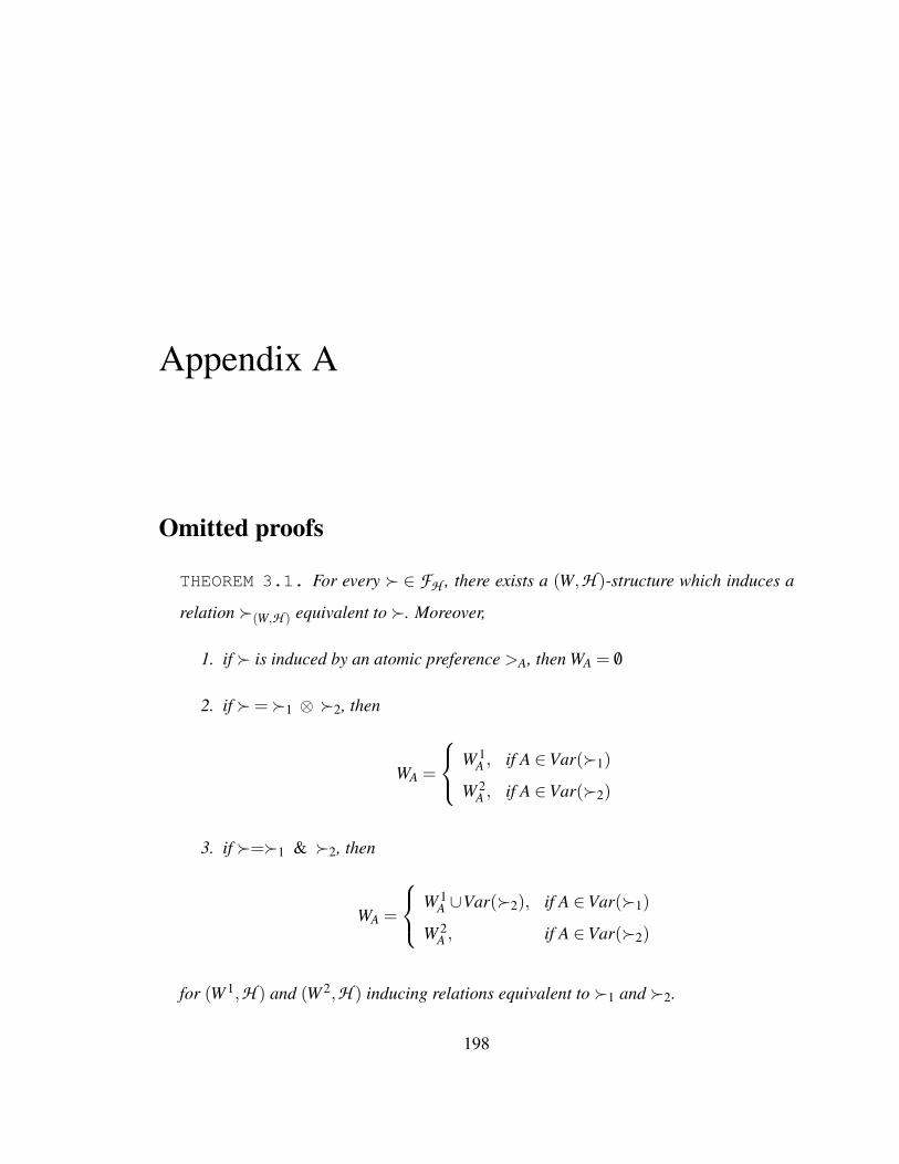
Appendix A
Omitted proofs
THEOREM 3.1. For every ∈ FH , there exists a (W,H )-structure which induces a
relation (W,H ) equivalent to . Moreover,
1. if is induced by an atomic preference >A, then WA = /0
2. if =1 ⊗ 2, then
WA =
W 1A , if A ∈Var(1)
W 2A , if A ∈Var(2)
3. if =1 & 2, then
WA =
W 1A ∪Var(2), if A ∈Var(1)
W 2A , if A ∈Var(2)
for (W 1,H ) and (W 2,H ) inducing relations equivalent to 1 and 2.
198

OMITTED PROOFS 199
PROOF
We show here that for any ∈ FH there exists W such that
≡ (W,H ) ≡ TC
⋃A∈Var()
pA
pA ≡ (o1,o2) | o1.A A o2.A ∩ ≈A−WA−A
We prove it by induction in the sizes of H and the corresponding A .
BASE STEP. Let H = >A and A = A. Then FH consists of a single p-skyline
relation which is induced by >A. Take WA = /0. Then
= (W,H ) ≡ TC(pA)
pA ≡ (o1,o2) | o1.A >A o2.A ∩ ≈A−WA−A
INDUCTIVE STEP. Now assume that the theorem holds for H and A of size up to n. Prove
that it holds for H and A of size n+1. Let = 1 ⊗ 2 (the case of = 1 & 2 is
similar). By the definition of p-skyline relations,
≡ (1 ∩ ≈Var(2)) ∪ (2 ∩ ≈Var(1)) ∪ (1 ∩ 2)
Thus, for two p-skyline relations 1 and 2 the inductive assumption implies that 1 and
2 can be represented by the structures (W 1,H 1) and (W 2,H 2) where H 1 and H 2 contain

OMITTED PROOFS 200
only the members of H for Var(1) and Var(2) correspondingly. That is,
1 = (W 1,H ) ≡ TC(⋃
A∈Var(1)
p1A) (7.1)
2 = (W 2,H ) ≡ TC(⋃
A∈Var(2)
p2A) (7.2)
where
p1A ≡ (o1,o2) | o1.A >A o2.A ∩ ≈Var(1)−W 1
A−A(7.3)
p2A ≡ (o1,o2) | o1.A >A o2.A ∩ ≈Var(2)−W 2
A−A(7.4)
Since is a p-skyline relation,
Var(1)∩Var(2) = /0. (7.5)
(7.5), (7.1), and (7.2) imply
≡ TC
⋃A∈Var(1)
p1A
∩ ≈Var(2) ∪ TC
⋃A∈Var(2)
p2A
∩ ≈Var(1) ∪
TC
⋃A∈Var(1)
p1A
∩TC
⋃A∈Var(2)
p2A
(7.6)

OMITTED PROOFS 201
or equivalently
≡ TC
⋃A∈Var(1)
p1A∩ ≈Var(2)
∪ TC
⋃A∈Var(2)
p2A∩ ≈Var(1)
∪TC
⋃A∈Var(1)
p1A
∩TC
⋃A∈Var(2)
p2A
(7.7)
Construct the function W as follows
WA =
W 1A , if A ∈Var(1)
W 2A , if A ∈Var(2)
.
Take (W,H ) induced by (W,H )
(W,H ) ≡ TC(⋃
A∈Ap∗A) (7.8)
for
p∗A ≡ (o1,o2) | o1.A >A o2.A ∩ ≈A−WA−A (7.9)
We prove that (W,H ) is equivalent to . Before going to the proof, notice that (7.7)
can be rewritten as
≡ TC
⋃A∈Var(1)
p∗A
∪TC
⋃A∈Var(2)
p∗A
∪TC
⋃A∈Var(1)
p1A
∩TC
⋃A∈Var(2)
p2A
(7.10)
1. Let o(W,H ) o′. Let (Σo,o′,Ψo,o′) be any derivation sequence for o(W,H ) o′. W.l.o.g.

OMITTED PROOFS 202
let Ψo,o′ = (A1, . . . ,Am), Σo,o′ = (o = o1,o2, . . . ,om,om+1 = o′), and
p∗A1(o1,o2), p∗A2
(o2,o3), . . . , p∗Am(om,om+1) (7.11)
By construction, each attribute Ai ∈ Ψo,o′ is either in Var(1) or Var(2). For any
such Ai, p∗Ai(oi,oi+1) implies oi oi+1 by (7.10). Therefore, (7.11) implies
o1 o2,o2 o3, ...,om om+1 (7.12)
Transitivity of p-skyline relations implies o1 om+1, i.e. o o′.
2. Let o o′. Then (7.10) leads to three cases
(a) (o,o′) ∈ TC(⋃
A∈Var(1) p∗A)
. Then o(W,H ) o′ by (7.8).
(b) (o,o′) ∈ TC(⋃
A∈Var(2) p∗A)
. Then o(W,H ) o′ by the same reasoning.
(c) (o,o′) ∈ TC(⋃
A∈Var(1) p1A
)∩TC
(⋃A∈Var(2) p2
A
).
In this case, (7.5) implies that there is an object o′′ whose values of Var(2) are
equal to those of o, and the values of Var(1) are equal to those of o′. Then we
have
(o,o′′) ∈ TC
⋃A∈Var(1)
p1A
∩ ≈Var(2)
(o′′,o′) ∈ TC
⋃A∈Var(2)
p1A
∩ ≈Var(1)

OMITTED PROOFS 203
or equivalently
(o,o′′) ∈ TC
⋃A∈Var(1)
p1A∩ ≈Var(2)
(o′′,o′) ∈ TC
⋃A∈Var(2)
p1A∩ ≈Var(1)
which implies by (7.9) and (7.8)
o(W,H ) o1,o1 (W,H ) o′
The transitivity of (W,H ) implies o(W,H ) o′.
LEMMA 3.3. Let for two p-skyline relations 1,2∈ FH , (W 1,H ) and (W 2,H ) be two
structures inducing relations equal to 1 and 2 correspondingly. Let for some A ∈ A ,
W 1A −W 2
A 6= /0. Then there is a pair o,o′ ∈U such that
o1 o′,o 62 o′
PROOF
We construct two tuples o and o′ such that o(W 1,H ) o′ (and thus o1 o′), and o 6(W 2,H ) o′
(and thus o 6(W 2,H ) o′).
For every attribute Ai ∈A , pick two values vAi,v′Ai∈DAi such that vAi >Ai v′Ai
. Construct
the tuples o and o′ as follows:
o.Ai =
vAi, if Ai = A,
vAi, if Ai ∈ A−A−W 1A ,
v′Ai, otherwise(Ai ∈W 1
A )
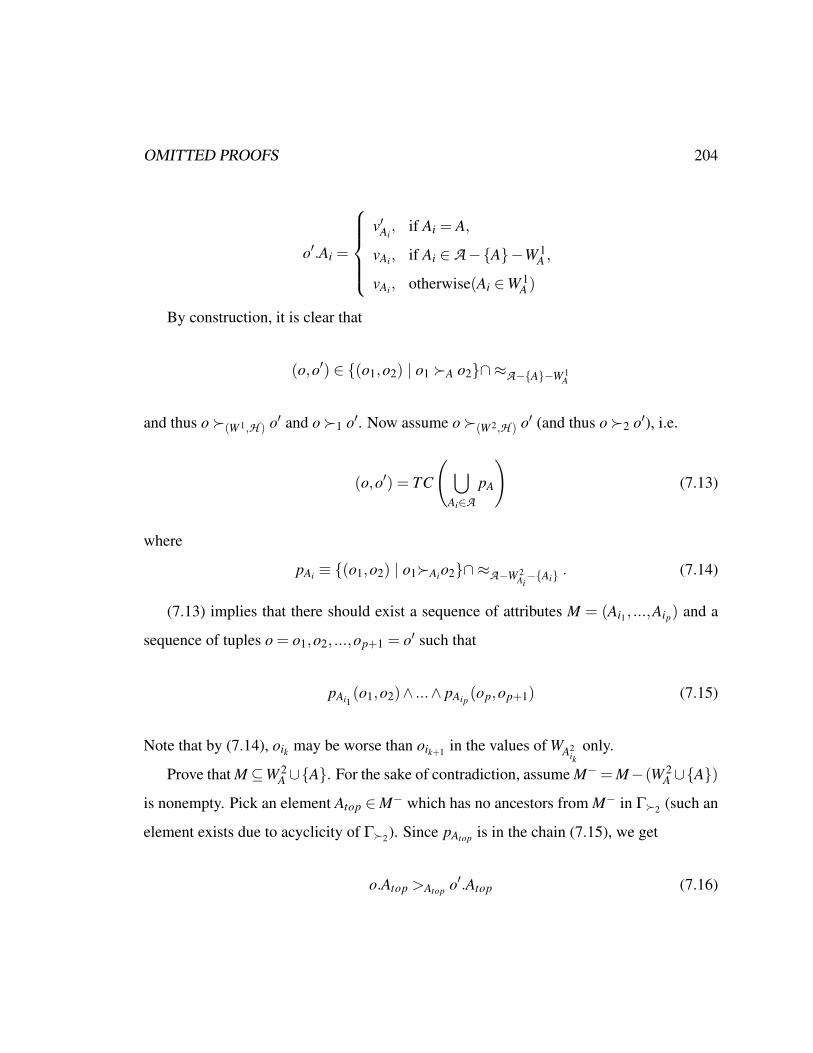
OMITTED PROOFS 204
o′.Ai =
v′Ai
, if Ai = A,
vAi, if Ai ∈ A−A−W 1A ,
vAi, otherwise(Ai ∈W 1A )
By construction, it is clear that
(o,o′) ∈ (o1,o2) | o1 A o2∩ ≈A−A−W 1A
and thus o(W 1,H ) o′ and o1 o′. Now assume o(W 2,H ) o′ (and thus o2 o′), i.e.
(o,o′) = TC
( ⋃Ai∈A
pA
)(7.13)
where
pAi ≡ (o1,o2) | o1Aio2∩ ≈A−W 2Ai−Ai . (7.14)
(7.13) implies that there should exist a sequence of attributes M = (Ai1, ...,Aip) and a
sequence of tuples o = o1,o2, ...,op+1 = o′ such that
pAi1(o1,o2)∧ ...∧ pAip
(op,op+1) (7.15)
Note that by (7.14), oik may be worse than oik+1 in the values of WA2ik
only.
Prove that M⊆W 2A ∪A. For the sake of contradiction, assume M−= M−(W 2
A ∪A)
is nonempty. Pick an element Atop ∈M− which has no ancestors from M− in Γ2 (such an
element exists due to acyclicity of Γ2). Since pAtop is in the chain (7.15), we get
o.Atop >Atop o′.Atop (7.16)

OMITTED PROOFS 205
By construction of o, o′ that implies Atop = A which is a contradiction. Thus, M ⊆W 2A ∪
A.
Now pick any B ∈W 1A −W 2
A . By construction of o,o′, o′.B B o.B. Therefore, there
is C ∈M such that B ∈W 2C . The transitivity of Γ2 implies B ∈W 2
A which contradicts the
initial assumption about B. Thus o 6(W 2,H ) o′ and o 62 o′
THEOREM 3.6. Let be a p-skyline relation with the p-graph Γ. Let also A,B,C,D
be disjoint node sets of Γ. Let the subgraphs of Γ induced by those node sets be
singletons or unions of at least two disjoint subgraphs. Then
(A,B) ∈ Γ ∧(C,D) ∈ Γ∧ (C,B) ∈ Γ⇒
(C,A) ∈ Γ∨ (A,D) ∈ Γ∨ (D,B) ∈ Γ
PROOF
Prove the theorem by contradiction. Let
(A,B) ∈ Γ ∧ (C,D) ∈ Γ∧ (C,B) ∈ Γ∧
(C,A) 6∈ Γ∧ (A,D) 6∈ Γ∧ (D,B) 6∈ Γ
The second part is equivalent to the following.
∃C ∈ C,A1,A2 ∈ A,D1,D2 ∈ D,B ∈ B(
(C,A2) 6∈ Γ∧ (C-A2)
(A1,D1) 6∈ Γ∧ (A1-D1)
(D2,B) 6∈ Γ) (D2-B)
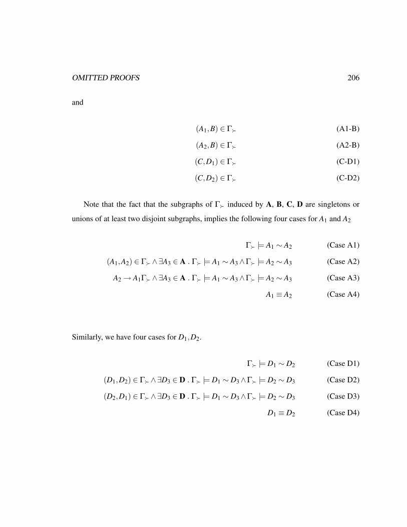
OMITTED PROOFS 206
and
(A1,B) ∈ Γ (A1-B)
(A2,B) ∈ Γ (A2-B)
(C,D1) ∈ Γ (C-D1)
(C,D2) ∈ Γ (C-D2)
Note that the fact that the subgraphs of Γ induced by A, B, C, D are singletons or
unions of at least two disjoint subgraphs, implies the following four cases for A1 and A2
Γ |= A1 ∼ A2 (Case A1)
(A1,A2) ∈ Γ∧∃A3 ∈ A . Γ |= A1 ∼ A3∧Γ |= A2 ∼ A3 (Case A2)
A2→ A1Γ∧∃A3 ∈ A . Γ |= A1 ∼ A3∧Γ |= A2 ∼ A3 (Case A3)
A1 ≡ A2 (Case A4)
Similarly, we have four cases for D1,D2.
Γ |= D1 ∼ D2 (Case D1)
(D1,D2) ∈ Γ∧∃D3 ∈ D . Γ |= D1 ∼ D3∧Γ |= D2 ∼ D3 (Case D2)
(D2,D1) ∈ Γ∧∃D3 ∈ D . Γ |= D1 ∼ D3∧Γ |= D2 ∼ D3 (Case D3)
D1 ≡ D2 (Case D4)

OMITTED PROOFS 207
Therefore, totally we have sixteen different cases, and we need to show that all of them lead
to contradictions. One can show that all of them contradict the Envelope property. We
demonstrate it for the case (A3-D2), while the other cases are handled similarly. In Figure
7-1, we show instances of the Envelope property. Recall that the Envelope property
says that if a graph has three certain edges, it must have at least one of other three edges.
The instances we show below lead to only one possible edge while the other two violate
some conditions above. The violated condition is shown below each corresponding edge.
Finally, we show that there is an unsatisfiable instance of the Envelope property.
We have automatically tested the other fifteen cases and showed that similar contradic-
tions can be derived for them, too.
Envelope condition first edge second edge third edge(A2,B), (C,D2), (C,B) (D2,B) (A2,D2) (C,A2)
(D2-B) (C-A2)(A2,D2), (C,D3), (C,D2) (D3,D2) (C,A2) (A2,D3)
(D3 ∼ D2) (C-A2)(A3,B), (A2,D2), (A2,B) (D2,B) (A2,A3) (A3,D2)
(D2-B) (A2 ∼ A3)(A3,D2), (A2,D3), (A2,D2) (A3,D3) (D3,D2) (A2,A3)
(D3 ∼ D2) (A2-A3)(A2,D3), (C,D1), (C,D3) (A2,D1) (C,A2) (D1,D3)
(C-A2) (D1 ∼ D3)(D1,D2), (A3,D3), (A3,D2) (D3,D2) (A3,D1) (D1,D3)
(D3 ∼ D2) (D1 ∼ D3)(A3,D1), (A2,A1), (A2,D1) (A2,A3) (A1,D1) (A3,A1)
(A2 ∼ A3) (A1-D1) (A3 ∼ A1)
Figure 7-1: Case A3-D2
LEMMA 3.4. Let ext be a full p-skyline extension of ∈ FH , and T be a normalized
syntax tree of . Let also (C1,C2) be a frontier pair of T w.r.t. Text . Denote the top and
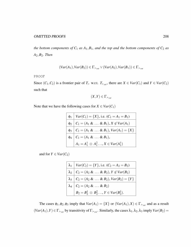
OMITTED PROOFS 208
the bottom components of C1 as A1,B1, and the top and the bottom components of C2 as
A2,B2. Then
(Var(A1),Var(B2)) ∈ Γext ∨ (Var(A2),Var(B1)) ∈ Γext
PROOF
Since (C1,C2) is a frontier pair of T w.r.t. Text , there are X ∈ Var(C1) and Y ∈ Var(C2)
such that
(X ,Y ) ∈ Γext
Note that we have the following cases for X ∈Var(C1)
φ1 Var(C1) = X, i.e. (C1 = A1 = B1)
φ2 C1 = (A1 & . . . & B1), X 6∈Var(A1)
φ3 C1 = (A1 & . . . & B1), Var(A1) = X
φ4 C1 = (A1 & . . . & B1),
A1 = A11 ⊗ A2
1 . . ., X ∈Var(A11)
and for Y ∈Var(C2)
λ1 Var(C2) = Y, i.e. (C2 = A2 = B2)
λ2 C2 = (A2 & . . . & B2), Y 6∈Var(B2)
λ3 C2 = (A2 & . . . & B2), Var(B2) = Y
λ4 C2 = (A2 & . . . & B2)
B2 = B12 ⊗ B2
2 . . ., Y ∈Var(B12).
The cases φ1,φ2,φ3 imply that Var(A1) = X or (Var(A1),X) ∈ Γext and as a result
(Var(A1),Y )∈ Γext by transitivity of Γext . Similarly, the cases λ1,λ2,λ3 imply Var(B2) =
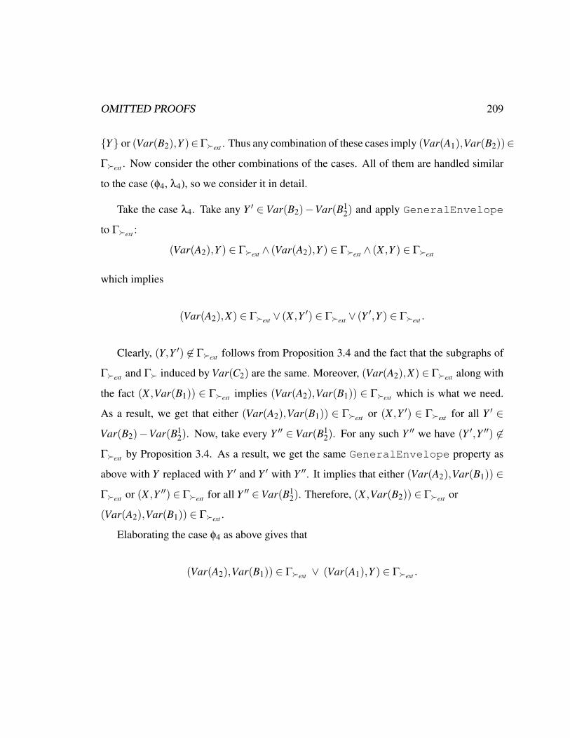
OMITTED PROOFS 209
Y or (Var(B2),Y )∈Γext . Thus any combination of these cases imply (Var(A1),Var(B2))∈
Γext . Now consider the other combinations of the cases. All of them are handled similar
to the case (φ4, λ4), so we consider it in detail.
Take the case λ4. Take any Y ′ ∈ Var(B2)−Var(B12) and apply GeneralEnvelope
to Γext :
(Var(A2),Y ) ∈ Γext ∧ (Var(A2),Y ) ∈ Γext ∧ (X ,Y ) ∈ Γext
which implies
(Var(A2),X) ∈ Γext ∨ (X ,Y ′) ∈ Γext ∨ (Y ′,Y ) ∈ Γext .
Clearly, (Y,Y ′) 6∈ Γext follows from Proposition 3.4 and the fact that the subgraphs of
Γext and Γ induced by Var(C2) are the same. Moreover, (Var(A2),X) ∈ Γext along with
the fact (X ,Var(B1)) ∈ Γext implies (Var(A2),Var(B1)) ∈ Γext which is what we need.
As a result, we get that either (Var(A2),Var(B1)) ∈ Γext or (X ,Y ′) ∈ Γext for all Y ′ ∈
Var(B2)−Var(B12). Now, take every Y ′′ ∈ Var(B1
2). For any such Y ′′ we have (Y ′,Y ′′) 6∈
Γext by Proposition 3.4. As a result, we get the same GeneralEnvelope property as
above with Y replaced with Y ′ and Y ′ with Y ′′. It implies that either (Var(A2),Var(B1)) ∈
Γext or (X ,Y ′′) ∈ Γext for all Y ′′ ∈Var(B12). Therefore, (X ,Var(B2)) ∈ Γext or
(Var(A2),Var(B1)) ∈ Γext .
Elaborating the case φ4 as above gives that
(Var(A2),Var(B1)) ∈ Γext ∨ (Var(A1),Y ) ∈ Γext .

OMITTED PROOFS 210
Combining these two results gives
(Var(A1),Var(B2)) ∈ Γext ∨ (Var(A2),Var(B1)) ∈ Γext .
LEMMA 4.1. Take a full p-skyline relation , a disjoint subsets G and W of a set of
objects O. Then the next two operations can be done in polynomial time.
1. Verifying if is optimal favoring G and disfavoring W in O;
2. Computing an optimal p-skyline relation ′∈ FH favoring G and disfavoring W in
O which is an extension of PROOF
To check if favors G and disfavors W in O, we need to compute w(O), check G ⊆
w(O), and verify that for every o ∈W , there is o′ ∈ G such that o′ o. It can clearly be
done in polynomial time. If any of these conditions fails, then is obviously not optimal.
Otherwise, we need to check if every its minimal extension favors G and disfavors W . Note
that since disfavors W in O, any its extension also disfavors W in O. Hence, is not
optimal if at least one minimal extension favors G in O, and it is optimal otherwise. Corol-
laries 3.5 and 3.6 imply that all minimal extension of can be computed in polynomial
time.
To construct an optimal extension ′ of , we can take , construct its every minimal
extension and verify if at least one of them favors G in O. If any of them does, we pick it
and repeat the same procedure for it. We do it until for some′ its every minimal extension
does not favor G in O. This implies that ′ is an optimal p-skyline relation favoring G and
disfavoring W in O. Moreover, ′ is a superset of by construction. Corollaries 3.5, 3.6,
and 3.7 imply that such a computation can be done in polynomial time.
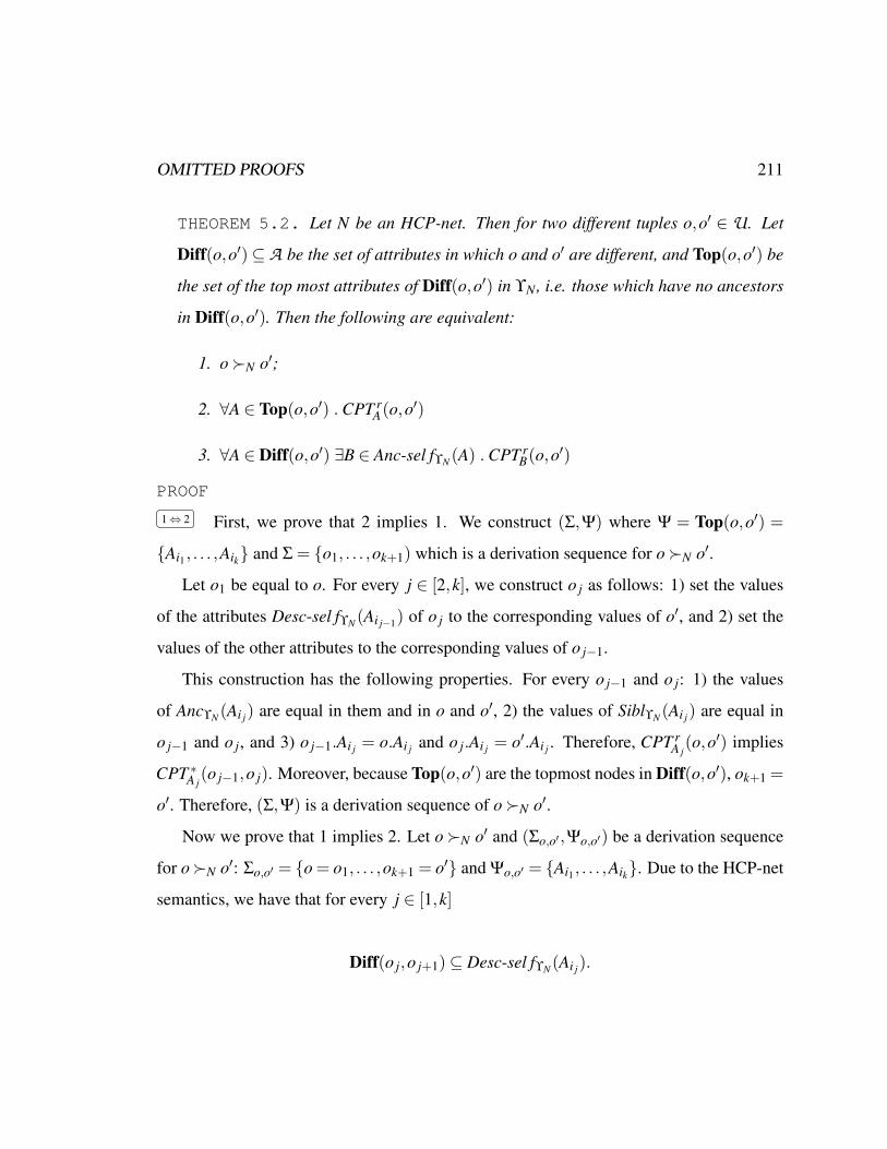
OMITTED PROOFS 211
THEOREM 5.2. Let N be an HCP-net. Then for two different tuples o,o′ ∈ U. Let
Diff(o,o′)⊆ A be the set of attributes in which o and o′ are different, and Top(o,o′) be
the set of the top most attributes of Diff(o,o′) in ϒN , i.e. those which have no ancestors
in Diff(o,o′). Then the following are equivalent:
1. oN o′;
2. ∀A ∈ Top(o,o′) . CPT rA(o,o′)
3. ∀A ∈ Diff(o,o′) ∃B ∈ Anc-sel fϒN (A) . CPT rB(o,o′)
PROOF
1⇔ 2 First, we prove that 2 implies 1. We construct (Σ,Ψ) where Ψ = Top(o,o′) =
Ai1, . . . ,Aik and Σ = o1, . . . ,ok+1) which is a derivation sequence for oN o′.
Let o1 be equal to o. For every j ∈ [2,k], we construct o j as follows: 1) set the values
of the attributes Desc-sel fϒN (Ai j−1) of o j to the corresponding values of o′, and 2) set the
values of the other attributes to the corresponding values of o j−1.
This construction has the following properties. For every o j−1 and o j: 1) the values
of AncϒN (Ai j) are equal in them and in o and o′, 2) the values of SiblϒN (Ai j) are equal in
o j−1 and o j, and 3) o j−1.Ai j = o.Ai j and o j.Ai j = o′.Ai j . Therefore, CPT rA j
(o,o′) implies
CPT ∗A j(o j−1,o j). Moreover, because Top(o,o′) are the topmost nodes in Diff(o,o′), ok+1 =
o′. Therefore, (Σ,Ψ) is a derivation sequence of oN o′.
Now we prove that 1 implies 2. Let oN o′ and (Σo,o′,Ψo,o′) be a derivation sequence
for oN o′: Σo,o′ = o = o1, . . . ,ok+1 = o′ and Ψo,o′ = Ai1, . . . ,Aik. Due to the HCP-net
semantics, we have that for every j ∈ [1,k]
Diff(o j,o j+1)⊆ Desc-sel fϒN (Ai j).

OMITTED PROOFS 212
Hence,
Top(o,o′)⊆ Diff(o,o′)⊆⋃
B∈Ψo,o′
Desc-sel fϒN (B)
We show that
no member B of Top(o,o′) has an ancestor in Ψo,o′ . (7.17)
Note that if some B ∈ Top(o,o′) has an ancestor C ∈ Ψo,o′ then CPT rC is not an SPO
or there is an ancestor D ∈ Ψo,o′ of C (which is also an ancestor of B) and so on. That
contradicts to the finiteness and SPO of ϒN . Hence, 7.17 holds, and all tuples in Σo,o′ are
equal in the ancestors of all the members of Top(o,o′).
Now take any A ∈ Top(o,o′). Take the sequence of the values of A in the tuples Σo,o′ .
Then for every pair a,a′ in this sequence (s.t. a precedes a′), a is preferred to a′ according
to Rq of the same q ∈ ΦA for all pairs (due to the argument above). By the transitivity of
Rq, Rq(o.A,o′.A). Therefore, CPT rA(o,o′).
2⇔ 3 First, let ∀A ∈ Top(o,o′) . CPT rA(o,o′). For contradiction, assume
∃B ∈ Diff(o,o′) ∀C ∈ Anc-sel fϒN (B) . ¬CPT rC(o,o′). (7.18)
Then any topmost element C of Anc-sel fϒN (B)∩Diff(o,o′) is also in Top(o,o′). Then
(7.18) implies ¬CPT rC(o,o′) which contradicts the initial assumption.
Now let
∀B ∈ Diff(o,o′) ∃C ∈ Anc-sel fϒN (B) . CPT rC(o,o′). (7.19)
For the sake of contradiction, assume
∃A ∈ Top(o,o′) . ¬CPT rA(o,o′). (7.20)

OMITTED PROOFS 213
Then (7.19) and (7.20) imply that there is C∈AncϒN (A) such that CPT rC(o,o′). That implies
o.C 6= o′.C, i.e. C ∈ Diff(o,o′). Then the fact that C is an ancestor of A in ϒA implies
A 6∈ Top(o,o′) which is a contradiction.