Predictive State Representations

Duke University Machine Learning Group

Discussion Leader: Kai Ni

September 09, 2005

Outline

• Predictive State Representations (PSR) Model

• Constructing a PSR from a POMDP

• Learning parameters for PSR

• Conclusions

Two Popular Methods

• There are two dominant approaches in controlling/AI area.

• The generative-model approach– Typified by POMDP, more general, unlimited memory;

– Strongly dependent on a good model of system.

• The history-based approach– Typified by k-order Markov methods, simple and effective;

– Limited by history extension.

The Position of PSR

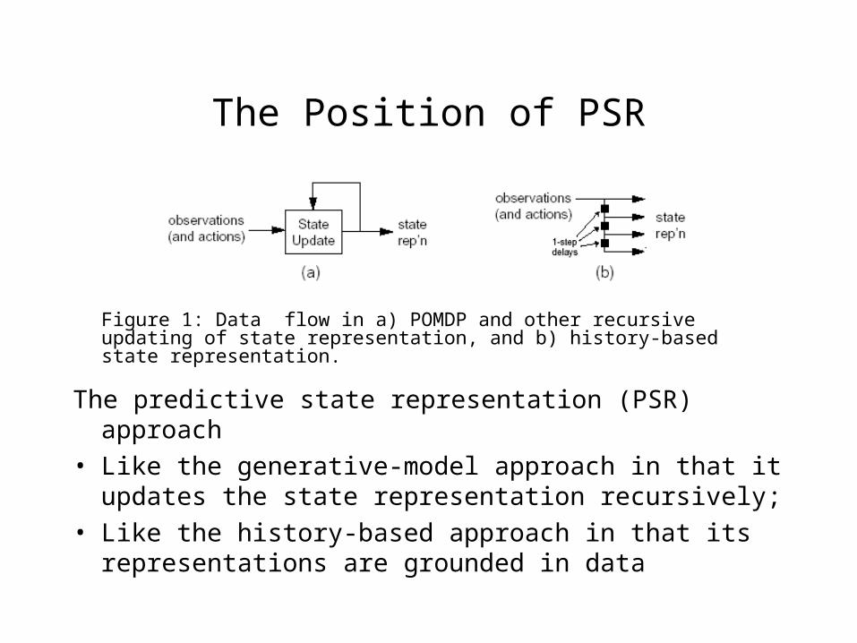
The predictive state representation (PSR) approach

• Like the generative-model approach in that it updates the state representation recursively;

• Like the history-based approach in that its representations are grounded in data

Figure 1: Data flow in a) POMDP and other recursive updating of state representation, and b) history-based state representation.

What is a PSR

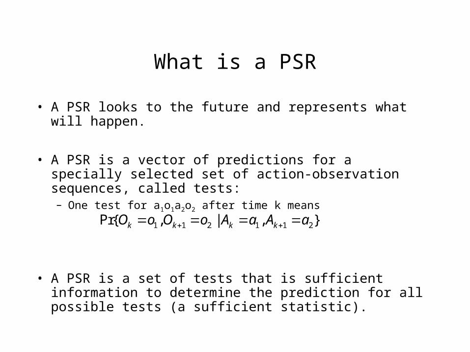
• A PSR looks to the future and represents what will happen.

• A PSR is a vector of predictions for a specially selected set of action-observation sequences, called tests:– One test for a1o1a2o2 after time k means

• A PSR is a set of tests that is sufficient information to determine the prediction for all possible tests (a sufficient statistic).

1 1 2 1 1 2Pr{ , | , }k k k kO o O o A a A a

The System-Dynamics Vector (1)

• Given an ordering over all possible tests t1t2…, the system’s probability distribution over all tests, defines an infinite system-dynamics vector d.

• The ith elements of d is the prediction of the ith test

• The predictions in d have some properties

1 11 1

1 1

( ) Pr( , , | , , )

k ki i k k

k ki

d p t o o o o a a a a

where t o a o a

The System-Dynamics Vector (2)

( )

0 1

Let ( ) be the set of tests whose action sequences equal

. Then , ( ) 1

, ( ) ( )

i

k

t T a

o O

i d

T a

a k a A p t

t a A p t p tao

Figure 2: a) Each of d’s entries corresponds to the prediction of the test. b)Properties of the predictions imply structure in d.

System-Dynamics Matrix (1)

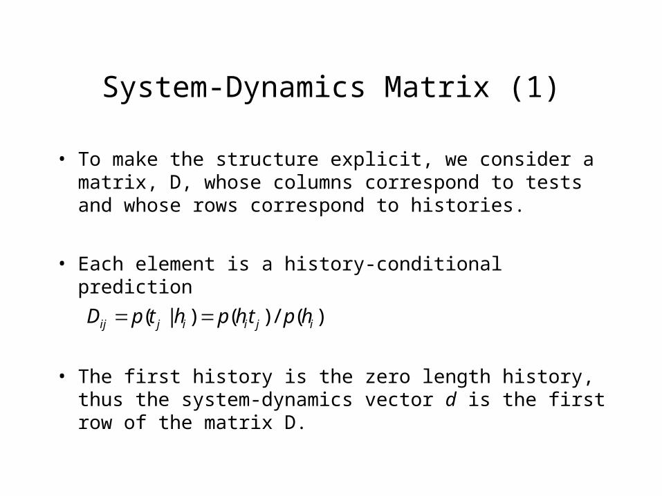
• To make the structure explicit, we consider a matrix, D, whose columns correspond to tests and whose rows correspond to histories.

• Each element is a history-conditional prediction

• The first history is the zero length history, thus the system-dynamics vector d is the first row of the matrix D.

( | ) ( ) / ( )ij j i i j iD p t h p h t p h

System-Dynamics Matrix (2)

Figure 3: The rows in the system-dynamics matrix correspond to all possible histories (pasts), while the columns correspond to all possible tests (futures). The entries in the matrix are the probabilities of futures given pasts.

• All the entries of matrix D are uniquely determined by the vector d because both the numerator and the denominator are elements of d.

POMDP and D

• The system-dynamics matrix D is not a model of the system but should be viewed as the system itself.

• D can be generated from a POMDP model by generating each test’s prediction as follows:

• Theorem: A POMDP with k nominal states cannot model a dynamical system with dimension greater than k. – The dimension of a dynamic system equal to the rank of D

1 1 11 1( | ) ( )n n nn n a a o a a op a o a o h b h T O T O 1

The Idea of Linear PSR

• For any D with rank k, there must exist k linearly independent columns and rows. We consider the set of columns and let the tests corresponding to these columns be Q = {q1 q2 … qk}, called core tests.

• For any h, the prediction vector p(Q|h) = [p(q1|h) … p(qk|h] is a predictive state representation. It forms a sufficient statistic for the system. All other tests can be calculated from the linear dependence

p(t|h) = p(Q|h)Tmt, where mt is the weight vector for test t.

Update the core tests

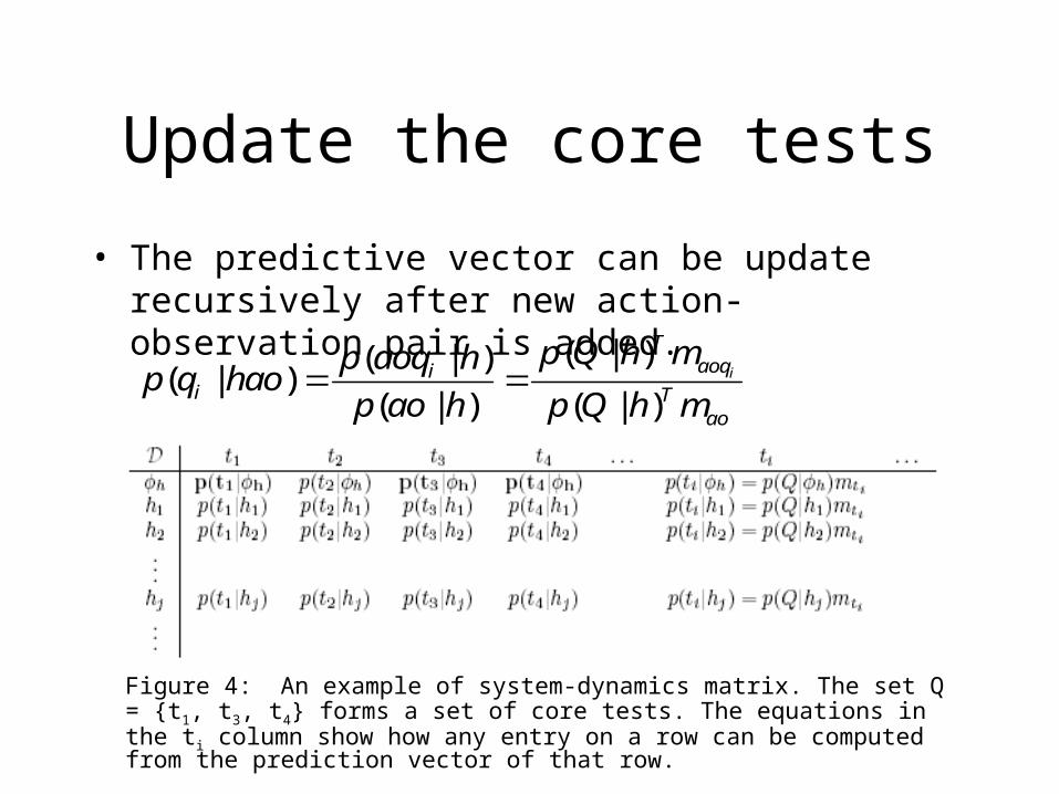
• The predictive vector can be update recursively after new action-observation pair is added.

( | )( | )( | )

( | ) ( | )i

Taoqi

i Tao

p Q h mp aoq hp q hao

p ao h p Q h m

Figure 4: An example of system-dynamics matrix. The set Q = {t1, t3, t4} forms a set of core tests. The equations in the ti column show how any entry on a row can be computed from the prediction vector of that row.

Constructing a PSR from a POMDP

• POMDP updates its belief state by computing

• Define a function u mapping tests to (1 x k) vectors by

u() = 1 and u(aot) = (TaOa,ou(t)T)T. We call u(t) the outcome vector for test t.

• A test t is linearly independent of a set of tests S if u(t) is linearly independent of the set of u(S).

( )( )

( )

a ao

a ao

b h T Ob hao

b h T O

1

Searching Algorithm

• The cardinality of Q is bounded by k and no test in Q is longer than k action-observation pairs.

• All other tests can be computed by 1 1

1 11 1( | ) ( | ) n n n n

n n T

a o a oa oP a o a o h p Q h M M m

Figure 5: Searching algorithm for finding a linear PSR from a POMDP.

An Example of PSR

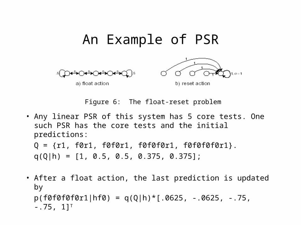
• Any linear PSR of this system has 5 core tests. One such PSR has the core tests and the initial predictions:

Q = {r1, f0r1, f0f0r1, f0f0f0r1, f0f0f0f0r1}.

q(Q|h) = [1, 0.5, 0.5, 0.375, 0.375];

• After a float action, the last prediction is updated by

p(f0f0f0f0r1|hf0) = q(Q|h)*[.0625, -.0625, -.75, -.75, 1]T

Figure 6: The float-reset problem

Learning PSR model

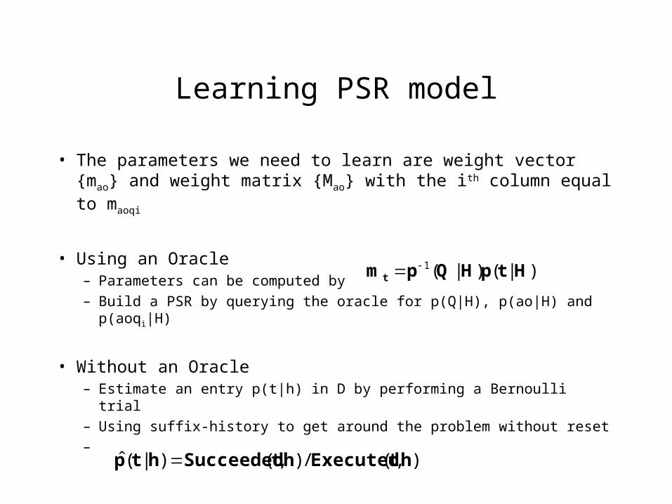
• The parameters we need to learn are weight vector {mao} and weight matrix {Mao} with the ith column equal to maoqi

• Using an Oracle– Parameters can be computed by

– Build a PSR by querying the oracle for p(Q|H), p(ao|H) and p(aoq i|H)

• Without an Oracle– Estimate an entry p(t|h) in D by performing a Bernoulli trial

– Using suffix-history to get around the problem without reset

–

)|()|(1 HtpHQpm t

),(/),()|(ˆ htExecutedhtSucceededhtp

TD (temporal difference) Learning

• Update long-term guess based on the next time step instead of waiting until the end.

• t = a1o1a2o2a3o3 and is the estimation of p(t|h). After takes action a1 and observe ok+1, TD estimation is:

and model parameters can be updated based on error.

• Expand the Q to include all suffixes of the core tests, called Y.

)|(ˆ htp

11

11

113322

,0

),|(ˆ)|(~

oo

ooohaoaoaphtp

k

k

))(

)|(()|(

hd

bWhQpghaoYp

ao

aoao

Result (1)

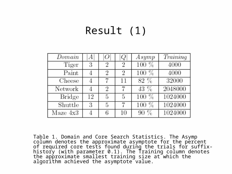
Table 1. Domain and Core Search Statistics. The Asymp column denotes the approximate asymptote for the percent of required core tests found during the trials for suffix-history (with parameter 0.1). The Training column denotes the approximate smallest training size at which the algorithm achieved the asymptote value.

Result (2)

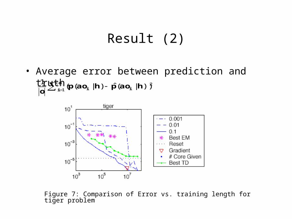
• Average error between prediction and truth.2

1))|(ˆ)|((

1haophaop

o i

o

i i

Figure 7: Comparison of Error vs. training length for tiger problem

Conclusion

• Predictive state representation (PSR) is a new way to model the dynamical systems. It is more general than both POMDPs and nth-order Markov models. PSR is grounded in data flow and is easy to learn.

• The system-dynamics matrix provides an interesting way of looking at discrete dynamical systems.

• The author propose suffix-history and TD algorithm for learning PSR without reset. Both of them have small prediction error.

Reference

• M. L. Littman, R. S. Sutton and S. Singh, “Predictive Representations of State”, NIPS 2002

• S. Singh, M. R. James and M. R. Rudary, “Predictive State Representations: A New Theory for Modeling Dynamical Systems”, UAI 2004

• B. Wolfe, M. R. James and S. Singh, “Learning Predictive State Representations in Dynamical Systems Without Reset”, ICML 2005