This document is downloaded from DR‑NTU (https://dr.ntu.edu.sg)Nanyang Technological University, Singapore.

Predictive Modelling and Analysis of ProcessParameters on Material Removal Characteristicsin Abrasive Belt Grinding Process

Pandiyan, Vigneashwara; Caesarendra, Wahyu; Tjahjowidodo, Tegoeh; Praveen,Gunasekaran

2017

Pandiyan, V., Caesarendra, W., Tjahjowidodo, T., & Praveen, G. (2017). Predictive Modellingand Analysis of Process Parameters on Material Removal Characteristics in Abrasive BeltGrinding Process. Applied Sciences, 7(4), 363‑.

https://hdl.handle.net/10356/88595

https://doi.org/10.3390/app7040363

© 2017 by The Authors. Licensee MDPI, Basel, Switzerland. This article is an open accessarticle distributed under the terms and conditions of the Creative Commons Attribution (CCBY) license (http://creativecommons.org/licenses/by/4.0/).

Downloaded on 13 Jan 2022 01:21:50 SGT

applied sciences

Article

Predictive Modelling and Analysis of ProcessParameters on Material Removal Characteristics inAbrasive Belt Grinding Process

Vigneashwara Pandiyan 1, Wahyu Caesarendra 2, Tegoeh Tjahjowidodo 1,* andGunasekaran Praveen 1

1 School of Mechanical and Aerospace Engineering, Nanyang Technological University, Singapore 639815,Singapore; vigneash002@e.ntu.edu.sg (V.P.); praveen008@e.ntu.edu.sg (G.P.)

2 Rolls-Royce@NTU Corporate Lab, Nanyang Technological University, Singapore 639815, Singapore;wcaesarendra@ntu.edu.sg

* Correspondence: ttegoeh@ntu.edu.sg; Tel.: +65-6790-4952

Academic Editor: David HeReceived: 28 February 2017; Accepted: 31 March 2017; Published: 6 April 2017

Abstract: The surface finishing and stock removal of complicated geometries is the principal objectivefor grinding with compliant abrasive tools. To understand and achieve optimum material removal ina tertiary finishing process such as Abrasive Belt Grinding, it is essential to look in more detail at theprocess parameters/variables that affect the stock removal rate. The process variables involved in abelt grinding process include the grit and abrasive type of grinding belt, belt speed, contact wheelhardness, serration, and grinding force. Changing these process variables will affect the performanceof the process. The literature survey on belt grinding shows certain limited understanding of materialremoval on the process variables. Experimental trials were conducted based on the Taguchi Method toevaluate the influence of individual and interactive process variables. Analysis of variance (ANOVA)was employed to investigate the belt grinding characteristics on material removal. This researchwork describes a systematic approach to optimise process parameters to achieve the desired stockremoval in a compliant Abrasive Belt Grinding process. Experimental study showed that the removedmaterial from a surface due to the belt grinding process has a non-linear relationship with the processvariables. In this paper, the Adaptive Neuro-Fuzzy Inference System (ANFIS) model is used todetermine material removal. Compared with the experimental results, the model accurately predictsthe stock removal. With further verification of the empirical model, a better understanding of thegrinding parameters involved in material removal, particularly the influence of the individual processvariables and their interaction, can be obtained.

Keywords: belt grinding; ANOVA; parameter analysis; material removal; predictive model

1. Introduction

Abrasive grinding is a widely employed finishing process, with abrasive grains being used asthe cutting edge to accomplish close tolerances and excellent dimensional correctness and surfaceintegrity. Abrasive Belt Grinding is a modification of the traditional grinding processes in which thecontact wheel is made of polymer backing material. The grinding belt is formed of abrasives coated ona backing material and fastened around at least two rotating polymer contact wheels, which make it acompliant tool, as shown in Figure 1. The soft contact polymer wheel enables this machining processto be appropriate to machine free-form surfaces due to its versatility, efficiency, and ability to machineworkpieces of intricate shapes and geometry [1]. Understanding of such a process is one of the mostdelicate problems in the industry due to the high complexity and nonlinearity. The process parameters

Appl. Sci. 2017, 7, 363; doi:10.3390/app7040363 www.mdpi.com/journal/applsci

Appl. Sci. 2017, 7, 363 2 of 17

affecting material removal belt grinding are that the complex and non-linear behaviour of the beltgrinding tool is predominantly dependent on the contacts amid the workpiece and abrasive belt.Jourani et al. [2] have presented a three-dimensional numerical model, which could determine pressuredistribution along with the distribution of real contact to study the contact between the belt constitutedby abrasive grains and the surface to understand the material removal mechanism. Zhang et al. [1]have stated that force distribution in the contact area between the workpiece and the elastic contactwheel determines the ratio of material removal in the belt grinding process. Ren et al. [3,4] developeda local process model to predict the material removal rate before machining, making it suiT for therobot programmer to optimize the tool path based on simulation results. Hamann [5] had proposed alinear mathematical model for material removal based on cutting parameters. However, the proposedequation is no longer adequate for intricate surfaces, as both complete removal and local removals arenot equivalently distributed in the entire contact area due to the complex geometry of the workpiecethat is machined. According to the brief literature review above, it can be concluded that most of theprevious research works concentrated on cutting path optimization, thereby making regular contactresulting in constant material removal [6–9]. Though the removal of material in the belt grindingprocess from the workpiece surface can be written as a function of several parameters, their influenceand interaction have not been reported in the literature that will be covered and bridged in thisresearch work. The material removal volume depends mainly on the contact force between the tooland the workpiece, the belt speed, and the feed rate in the tangential direction. The influences ofthese parameters on the material removal rate were examined experimentally. Orthogonal arrays ofTaguchi, analysis of variance (ANOVA), and regression analyses are employed to analyse the effect ofthe belt grinding parameters on the depth of cut, i.e., metal removal rate. The Taguchi Method usesorthogonal arrays in experimental design for a significant reduction in the number of experimentalruns to find the optimal solution. Taguchi methods have been widely utilised in engineering analysis toobtain information about the behaviour of a given process [10]. ANOVA is a statistical based analysisemployed to indicate the impact of process parameters on the process output and helps in predictingthe significance of all factors and their interactions [11]. In this research, we have also proposed anumerical model to predict material removal as a function of process parameters, namely, hardness,force, rotation speed, grit size, and feed rate, based on the Adaptive Neuro-Fuzzy Inference System(ANFIS). The ANFIS technique has been used in the past for the prediction and modelling of materialremoval as a function of the process parameters [12,13]. The Adaptive Neuro-Fuzzy Inference System(ANFIS) conjoins the benefits of the neural network and fuzzy systems [14]. When experimental dataand model results are compared, it is observed that the developed regression model is within the limitsof the acceptable error.

Appl. Sci. 2017, 7, 363 2 of 17

process parameters affecting material removal belt grinding are that the complex and non-linear

behaviour of the belt grinding tool is predominantly dependent on the contacts amid the workpiece

and abrasive belt. Jourani et al. [2] have presented a three-dimensional numerical model, which could

determine pressure distribution along with the distribution of real contact to study the contact

between the belt constituted by abrasive grains and the surface to understand the material removal

mechanism. Zhang et al. [1] have stated that force distribution in the contact area between the

workpiece and the elastic contact wheel determines the ratio of material removal in the belt grinding

process. Ren et al. [3,4] developed a local process model to predict the material removal rate before

machining, making it suiT for the robot programmer to optimize the tool path based on simulation

results. Hamann [5] had proposed a linear mathematical model for material removal based on cutting

parameters. However, the proposed equation is no longer adequate for intricate surfaces, as both

complete removal and local removals are not equivalently distributed in the entire contact area due

to the complex geometry of the workpiece that is machined. According to the brief literature review

above, it can be concluded that most of the previous research works concentrated on cutting path

optimization, thereby making regular contact resulting in constant material removal [6–9]. Though

the removal of material in the belt grinding process from the workpiece surface can be written as a

function of several parameters, their influence and interaction have not been reported in the literature

that will be covered and bridged in this research work. The material removal volume depends mainly

on the contact force between the tool and the workpiece, the belt speed, and the feed rate in the

tangential direction. The influences of these parameters on the material removal rate were examined

experimentally. Orthogonal arrays of Taguchi, analysis of variance (ANOVA), and regression

analyses are employed to analyse the effect of the belt grinding parameters on the depth of cut, i.e.,

metal removal rate. The Taguchi Method uses orthogonal arrays in experimental design for a

significant reduction in the number of experimental runs to find the optimal solution. Taguchi

methods have been widely utilised in engineering analysis to obtain information about the behaviour

of a given process [10]. ANOVA is a statistical based analysis employed to indicate the impact of

process parameters on the process output and helps in predicting the significance of all factors and

their interactions [11]. In this research, we have also proposed a numerical model to predict material

removal as a function of process parameters, namely, hardness, force, rotation speed, grit size, and

feed rate, based on the Adaptive Neuro-Fuzzy Inference System (ANFIS). The ANFIS technique has

been used in the past for the prediction and modelling of material removal as a function of the process

parameters [12,13]. The Adaptive Neuro-Fuzzy Inference System (ANFIS) conjoins the benefits of the

neural network and fuzzy systems [14]. When experimental data and model results are compared, it

is observed that the developed regression model is within the limits of the acceptable error.

Figure 1. Principle of belt grinding process.

The paper is organised as follows; a brief overview of the Abrasive Belt Grinding process and

the problem statement is presented in Section 1, followed by a brief outline of the belt grinding

Figure 1. Principle of belt grinding process.

Appl. Sci. 2017, 7, 363 3 of 17

The paper is organised as follows; a brief overview of the Abrasive Belt Grinding process and theproblem statement is presented in Section 1, followed by a brief outline of the belt grinding processand the Adaptive Neuro-fuzzy Inference System (ANFIS) in Section 2. The machining conditions,experimental setup, process parameter and the Taguchi orthogonal array design to minimise thenumber of grinding experiments are reported in Section 3. The results of the belt grinding tests areanalysed using the signal to noise ratio (S/N) and ANOVA in Section 4, followed by a summary of thepredictive modelling of material removal using ANFIS. Finally, the conclusions of this research workare reviewed in Section 5.

2. Theoretical Basis

2.1. Abrasive Belt Grinding Process

Abrasive Belt Grinding is a tertiary polishing process with a geometrically indeterminatemachining edge with multiple grains. The belt grinding setup has an elastic contact roller wheelmade up of thermosetting polyurethane elastomer, which can be deformed to assist the coated abrasivebelt that functions as the cutting edge, as illustrated in Figure 1. Compliant belt grinding correspondsto elastic grinding and has the capabilities of grinding, milling, and polishing [15].

The belt grinding process has characteristics of good workpiece-shape adaptability with uniformmaterial removal, low grinding temperature, maintenance of residual compressive stresses, andresistance to workpiece burning like any other tertiary finishing process. The belt grinding process canquickly generate surfaces with high levels of precision and smoothness. Presently, about one-thirdof abrasive wheel grinding has been substituted by belt grinding [15]. Similar to any other abrasivemachining process, many process parameters in belt grinding impact the last ground surface quality,including the grinding belt topography features and cutting parameters. The process parametersinclude belt speed, belt preloaded tension, the force imparted, feed rate, workpiece geometry, polymerhardness, and belt topography features such as grit size [3]. Hamann [5] had proposed a linearmathematical model as shown below as Equation (1), which states that the overall material removalrate (MRR) r is either relative or inversely proportional to parameters such as CA (constant of thegrinding process), KA (combination constant of resistance factor of the work coupon and grindingability factor of the belt), kt (belt wear factor), Vb (grinding rate), Vw (feed-in rate), Lw (machiningwidth), and FA (normal force).

r = CA.KA.kt.Vb

Vw.Lw.FA (1)

The material removal intensifies when the number of the interactions of the abrasive grains perunit time gets maximised [16]. Therefore it is evident that material removal is directly proportionalto the cutting speed (grinding rate) of the polymer contact wheel on the belt grinder. The depth ofpenetration depends on the topography and the geometry of the belt/wheel surfaces, which serves asan undefined cutting-edge. The coarser grain sizes exhibit a greater ability to achieve higher cuttingdepth, which results in higher material removal than finer sizes. Material removal increases with ahigher dwell time of interaction between the cutting grain edges, and workpiece surface, i.e., materialremoval, is inversely proportional to the feed-in rate [16]. Adequate force is required for the cuttingedge to penetrate deeply into the workpiece to achieve grain cutting depth resulting in materialremoval. The penetration depth of the grains into the work coupon surface predominantly depends onthe force imparted for grinding [16]. Belt finishing with contact wheels of different hardnesses resultsin dynamic changes in contact pressure, leading to a change in the mechanism of wear. This hints thatthe parameters discussed govern the belt grinding process, and changing any of the parameters willhave a resultant shift in the output. Stock removal commonly requires a harder polymer contact wheel,coarse abrasive grains, greater force, reduced feed, and better cutting speed. Finishing requires the useof a softer contact wheel and fine grade abrasive grains. However, the degree of the effect will varyparameter to parameter. The amount of material removed from the workpiece surface results from the

Appl. Sci. 2017, 7, 363 4 of 17

distinct local contact conditions, which are completely influenced by the process parameters/variables.The relationship between the material removal rate and process parameters is not well grasped, eventhough machining by belt grinding is remarkably straightforward and inexpensive. Belt grinding isused in industries based on operator’s skill and knowledge, making the process inherently exhibitpoor stability and reproducibility.

2.2. Adaptive Neuro-Fuzzy Inference System

The Adaptive Neuro-Fuzzy Inference System (ANFIS) is a blend of the neural network and fuzzyinference system. Fuzzy inference systems have no learning capabilities regarding the input-outputspace and no standard tuning methods for their rule bases, which make system adaptations difficult.The ANFIS technique offered a method for the fuzzy systems to acquire knowledge regarding thedataset to calculate the membership function parameters that permitted Fuzzy Inference System(FIS) for automatic system adaption. ANFIS architecture is a superimposition of FIS on the ArtificialNeural Network (ANN) architecture, which will enable FIS to optimise its rule base based on theoutput to learn like an ANN eliminating its inherent disadvantage. The ANFIS algorithm has anin-built advantage compared to fuzzy models as it holds the learning competencies of the ANN, whichaugments the system performance using a priori understanding [17]. Using an input and outputspace relation, ANFIS forms an FIS, the membership function of which is altered by exploiting theback-propagation algorithm and least square method available with ANN [18].

In this section, the ANFIS architecture and its learning algorithm for the Sugeno fuzzy model willbe described primarily. The ANFIS architecture is shown in Figure 2; ANFIS normally has five layersof neurons, of which neurons in the same layer are of the same function family. Assume that the FISunder consideration has two inputs, x and y, which form two fuzzy if–then rules based on first-orderSugeno fuzzy model [19].

Rule 1: If x is A1 and y is B1, then f 1 = p1x +q1y + r1;Rule 2: If x is A2 and y is B2, then f 2 = p2x +q2y + r2;where p1, p2, q1, q2, r1, and r2 are linear parameters and A1, A2, B1, and B2 are nonlinear parameters.The output of the ith node in layer 1 is denoted as O

l,i.

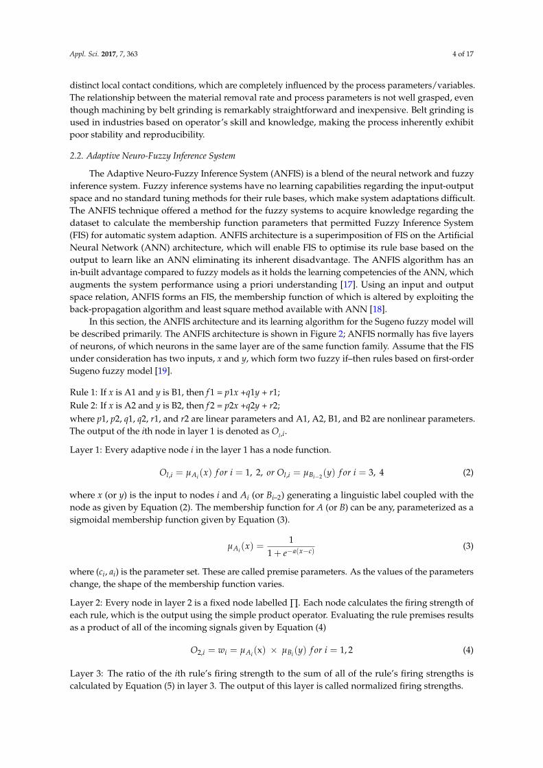
Layer 1: Every adaptive node i in the layer 1 has a node function.

Ol,i = µAi (x) f or i = 1, 2, or Ol,i = µBi−2(y) f or i = 3, 4 (2)

where x (or y) is the input to nodes i and Ai (or Bi–2) generating a linguistic label coupled with thenode as given by Equation (2). The membership function for A (or B) can be any, parameterized as asigmoidal membership function given by Equation (3).

µAi (x) =1

1 + e−a(x−c)(3)

where (ci, ai) is the parameter set. These are called premise parameters. As the values of the parameterschange, the shape of the membership function varies.

Layer 2: Every node in layer 2 is a fixed node labelled ∏. Each node calculates the firing strength ofeach rule, which is the output using the simple product operator. Evaluating the rule premises resultsas a product of all of the incoming signals given by Equation (4)

O2,i = wi = µAi (x) × µBi (y) f or i = 1, 2 (4)

Layer 3: The ratio of the ith rule’s firing strength to the sum of all of the rule’s firing strengths iscalculated by Equation (5) in layer 3. The output of this layer is called normalized firing strengths.

Appl. Sci. 2017, 7, 363 5 of 17

O3,i = wi =wi

Σ2i wi

=wi

w1 + w2i = 1, 2 (5)

Layer 4: Every node i in layer 4 is an adaptive node with a node function. The nodes computea parameter function on the layer output. Parameters in this layer will be referred to asconsequent parameters.

O4,i = wi fi = wi(pix + qiy + ri) (6)

where wi is a normalised firing strength from layer 3 and (pi, qi, ri) is the parameter set for the node.

Layer 5: This layer has a fixed single node labelled Σ, which computes the overall output as thesummation of all of the incoming signals, as shown in Equation (7). The Σ gives the overall output ofthe constructed adaptive network, having same functionality as the Sugeno fuzzy model.

O5,i = ∑i

wi fi =∑i wi fi

∑i wi(7)

From Figure 2, it can be noticed that the input membership functions of the Takagi-Sugeno modelare non-linear, whereas the output membership functions are linear.

Appl. Sci. 2017, 7, 363 5 of 17

where wi is a normalised firing strength from layer 3 and (pi, qi, ri) is the parameter set for the node.

Layer 5: This layer has a fixed single node labelled Σ, which computes the overall output as the

summation of all of the incoming signals, as shown in Equation (7). The Σ gives the overall output of

the constructed adaptive network, having same functionality as the Sugeno fuzzy model.

𝑂5,𝑖 = ∑ ��𝑖𝑓𝑖

𝑖

=∑ 𝑤𝑖𝑓𝑖𝑖

∑ 𝑤𝑖𝑖 (7)

From Figure 2, it can be noticed that the input membership functions of the Takagi-Sugeno

model are non-linear, whereas the output membership functions are linear.

Figure 2. Adaptive neuro-fuzzy inference system structure.

3. Experimental Procedures

3.1. Experiment Design Based on Taguchi Method

3.1.1. Experimental Setup

Belt grinding is a modification of the traditional grinding processes, with the contact wheel being

made of compliant polymer material. The abrasive belt sander, as shown in Figure 3, is customised

with a fixture design such that it can be used as a belt grinding tool. A belt sander is an electrically

powered abrasive belt tool that can be run at different variable speeds at unloading conditions. Ester

polyurethane polymer of different Shore A hardnesses is used as a contact wheel, which forms the

part of the contact arm, which is used as the machining end of the custom belt grinder setup, as shown

in Figure 3. The use of robots or multiple-axes machining centres improves the finishing efficiency.

Figure 3. Belt Sander customised to perform grinding experimental trials.

The experimental trials were conducted on coupling the belt sander and an ABB 6660-205-193

multi-axes robot using a suitable fixture, as shown in Figure 4. The ABB 6660-205-193 has a parallel

Figure 2. Adaptive neuro-fuzzy inference system structure.

3. Experimental Procedures

3.1. Experiment Design Based on Taguchi Method

3.1.1. Experimental Setup

Belt grinding is a modification of the traditional grinding processes, with the contact wheel beingmade of compliant polymer material. The abrasive belt sander, as shown in Figure 3, is customisedwith a fixture design such that it can be used as a belt grinding tool. A belt sander is an electricallypowered abrasive belt tool that can be run at different variable speeds at unloading conditions. Esterpolyurethane polymer of different Shore A hardnesses is used as a contact wheel, which forms the partof the contact arm, which is used as the machining end of the custom belt grinder setup, as shown inFigure 3. The use of robots or multiple-axes machining centres improves the finishing efficiency.

The experimental trials were conducted on coupling the belt sander and an ABB 6660-205-193multi-axes robot using a suitable fixture, as shown in Figure 4. The ABB 6660-205-193 has a parallelarm structure, powerful gears, and motors for handling fluctuating process forces prevalent withinapplications such as milling, deburring, and grinding. An ATI force sensor (Omega 160) connects thefixture and the robot arm end effector. This is accomplished by mounting the force sensor to the ABB

Appl. Sci. 2017, 7, 363 6 of 17

robots end-effector and then attaching the customised belt grinding tool to the force sensor, as shownin Figure 4. The robot controller continuously receives the force/torque signal, compares it with theusers input, and achieves force compensation. The system is close looped, and this ensures that theforce programmed and the force exerted are the same. The robot arm is primarily used for toolpathcontrol and force control.

Appl. Sci. 2017, 7, 363 5 of 17

where wi is a normalised firing strength from layer 3 and (pi, qi, ri) is the parameter set for the node.

Layer 5: This layer has a fixed single node labelled Σ, which computes the overall output as the

summation of all of the incoming signals, as shown in Equation (7). The Σ gives the overall output of

the constructed adaptive network, having same functionality as the Sugeno fuzzy model.

𝑂5,𝑖 = ∑ ��𝑖𝑓𝑖

𝑖

=∑ 𝑤𝑖𝑓𝑖𝑖

∑ 𝑤𝑖𝑖 (7)

From Figure 2, it can be noticed that the input membership functions of the Takagi-Sugeno

model are non-linear, whereas the output membership functions are linear.

Figure 2. Adaptive neuro-fuzzy inference system structure.

3. Experimental Procedures

3.1. Experiment Design Based on Taguchi Method

3.1.1. Experimental Setup

Belt grinding is a modification of the traditional grinding processes, with the contact wheel being

made of compliant polymer material. The abrasive belt sander, as shown in Figure 3, is customised

with a fixture design such that it can be used as a belt grinding tool. A belt sander is an electrically

powered abrasive belt tool that can be run at different variable speeds at unloading conditions. Ester

polyurethane polymer of different Shore A hardnesses is used as a contact wheel, which forms the

part of the contact arm, which is used as the machining end of the custom belt grinder setup, as shown

in Figure 3. The use of robots or multiple-axes machining centres improves the finishing efficiency.

Figure 3. Belt Sander customised to perform grinding experimental trials.

The experimental trials were conducted on coupling the belt sander and an ABB 6660-205-193

multi-axes robot using a suitable fixture, as shown in Figure 4. The ABB 6660-205-193 has a parallel

Figure 3. Belt Sander customised to perform grinding experimental trials.

Appl. Sci. 2017, 7, 363 6 of 17

arm structure, powerful gears, and motors for handling fluctuating process forces prevalent within

applications such as milling, deburring, and grinding. An ATI force sensor (Omega 160) connects the

fixture and the robot arm end effector. This is accomplished by mounting the force sensor to the ABB

robots end-effector and then attaching the customised belt grinding tool to the force sensor, as shown

in Figure 4. The robot controller continuously receives the force/torque signal, compares it with the

users input, and achieves force compensation. The system is close looped, and this ensures that the

force programmed and the force exerted are the same. The robot arm is primarily used for toolpath

control and force control.

Figure 4. Experimental setup for compliant Abrasive Belt Grinding.

3.1.2. Toolpath Planning

Force control is essential for avoiding over and under-cutting of the material. Force control is

particularly used for uniform material removal along the whole toolpath. Such an adaptive tool for

path generation in the system was realised with (ATI Omega 160) force control in the experimental

trials. A constant contact force throughout the abrasive belt finishing the process in the normal

direction (Z-axis) is achieved by using a force sensor (ATI Omega 160) attached to the end effector of

the robotic arm of an ABB 6660 robot. The force sensor maintains an adequate in-feed in the normal

direction. Tool path planning has five different zones, as shown in Figure 5. Zone A and Zone B are

when the abrasive belt tool enters the machining region, zone C is where the actual machining

happens in force control mode, and zones D and E are where the abrasive belt tool exits the machining

region. ABB Robot Studio executes tool path planning. Most of belt grinding processes are done on

complicated geometries, and maintaining uniform material removal can be realised only when tool

centre point (machining end) interacts with the surface normally, which is the current industrial

practice employing highly automatic robotic arm manipulators.

Figure 4. Experimental setup for compliant Abrasive Belt Grinding.

3.1.2. Toolpath Planning

Force control is essential for avoiding over and under-cutting of the material. Force control isparticularly used for uniform material removal along the whole toolpath. Such an adaptive tool forpath generation in the system was realised with (ATI Omega 160) force control in the experimentaltrials. A constant contact force throughout the abrasive belt finishing the process in the normaldirection (Z-axis) is achieved by using a force sensor (ATI Omega 160) attached to the end effector ofthe robotic arm of an ABB 6660 robot. The force sensor maintains an adequate in-feed in the normaldirection. Tool path planning has five different zones, as shown in Figure 5. Zone A and Zone Bare when the abrasive belt tool enters the machining region, zone C is where the actual machininghappens in force control mode, and zones D and E are where the abrasive belt tool exits the machiningregion. ABB Robot Studio executes tool path planning. Most of belt grinding processes are doneon complicated geometries, and maintaining uniform material removal can be realised only when

Appl. Sci. 2017, 7, 363 7 of 17

tool centre point (machining end) interacts with the surface normally, which is the current industrialpractice employing highly automatic robotic arm manipulators.Appl. Sci. 2017, 7, 363 7 of 17

Figure 5. Toolpath planning in force control mode by ABB Robot Studio.

3.1.3. Taguchi Based DoE (Design of Experiments)

As the knowledge of the likely interactions of the belt grinding parameters was not known

initially, trials were planned using Taguchi orthogonal array design, showing only the effects of the

individual parameters. To evaluate the effect of the belt grinding process parameters on material

removal, Taguchi’s L27 orthogonal array (five-factor, three-level) model is selected, and experiments

were performed based on it. In this study, the process parameters such as grit size, rubber shore A

hardness, force, feed, and wheel speed are considered to analyse material removal. Table 1 shows a

summary of process parameters and their level used for performing grinding trials. The experimental

layout for the five cutting parameters using the L27 orthogonal array is provided in Table 2. The

mean S/N ratio for each level of the other machining parameters is assessed based on the material

removal, i.e., depth of cut, and a greater S/N ratio corresponds to better material removal

characteristics.

Table 1. Belt grinding parameters and their levels.

Parameter Unit Levels

L1 L2 L3

RPM (m/min) 250 500 700

Feed (mm/s) 10 20 30

Force (N) 10 20 30

Rubber hardness (Shore A) 30 60 90

Grit Size - 60 120 220

3.2. Experimental Conditions

The experimental studies were done on a belt grinding setup based on settings of machining

parameters, which were defined by using the Taguchi experimental design method. In addition, the

test conditions listed below were maintained constantly throughout to achieve a controlled

experimental trial.

• The contact head of the belt grinder is kept at normal angle to keep uniformity in contact

conditions throughout machining.

• Tool wear effect was ignored as the tests were conducted in the useful lifetime of the belt tool.

• The surface condition of the machined aluminium 6061 coupons was uniform with a surface

roughness of 0.8 microns (μm).

• Experiments are carried out in dry conditions.

• Experiments were carried out with three passes for each trial. On each pass, the depth of cut was

measured at three different locations, as shown in Figure 6, resulting in nine measurements.

According to the parameter combinations from the Taguchi method, which obtained 27 trials as

presented in Table 2, 243 depth of cut readings were obtained.

Figure 5. Toolpath planning in force control mode by ABB Robot Studio.

3.1.3. Taguchi Based DoE (Design of Experiments)

As the knowledge of the likely interactions of the belt grinding parameters was not knowninitially, trials were planned using Taguchi orthogonal array design, showing only the effects of theindividual parameters. To evaluate the effect of the belt grinding process parameters on materialremoval, Taguchi’s L27 orthogonal array (five-factor, three-level) model is selected, and experimentswere performed based on it. In this study, the process parameters such as grit size, rubber shore Ahardness, force, feed, and wheel speed are considered to analyse material removal. Table 1 shows asummary of process parameters and their level used for performing grinding trials. The experimentallayout for the five cutting parameters using the L27 orthogonal array is provided in Table 2. The meanS/N ratio for each level of the other machining parameters is assessed based on the material removal,i.e., depth of cut, and a greater S/N ratio corresponds to better material removal characteristics.

Table 1. Belt grinding parameters and their levels.

Parameter UnitLevels

L1 L2 L3

RPM (m/min) 250 500 700Feed (mm/s) 10 20 30Force (N) 10 20 30

Rubber hardness (Shore A) 30 60 90Grit Size - 60 120 220

3.2. Experimental Conditions

The experimental studies were done on a belt grinding setup based on settings of machiningparameters, which were defined by using the Taguchi experimental design method. In addition,the test conditions listed below were maintained constantly throughout to achieve a controlledexperimental trial.

• The contact head of the belt grinder is kept at normal angle to keep uniformity in contact conditionsthroughout machining.

• Tool wear effect was ignored as the tests were conducted in the useful lifetime of the belt tool.• The surface condition of the machined aluminium 6061 coupons was uniform with a surface

roughness of 0.8 microns (µm).

Appl. Sci. 2017, 7, 363 8 of 17

• Experiments are carried out in dry conditions.• Experiments were carried out with three passes for each trial. On each pass, the depth of cut

was measured at three different locations, as shown in Figure 6, resulting in nine measurements.According to the parameter combinations from the Taguchi method, which obtained 27 trials aspresented in Table 2, 243 depth of cut readings were obtained.

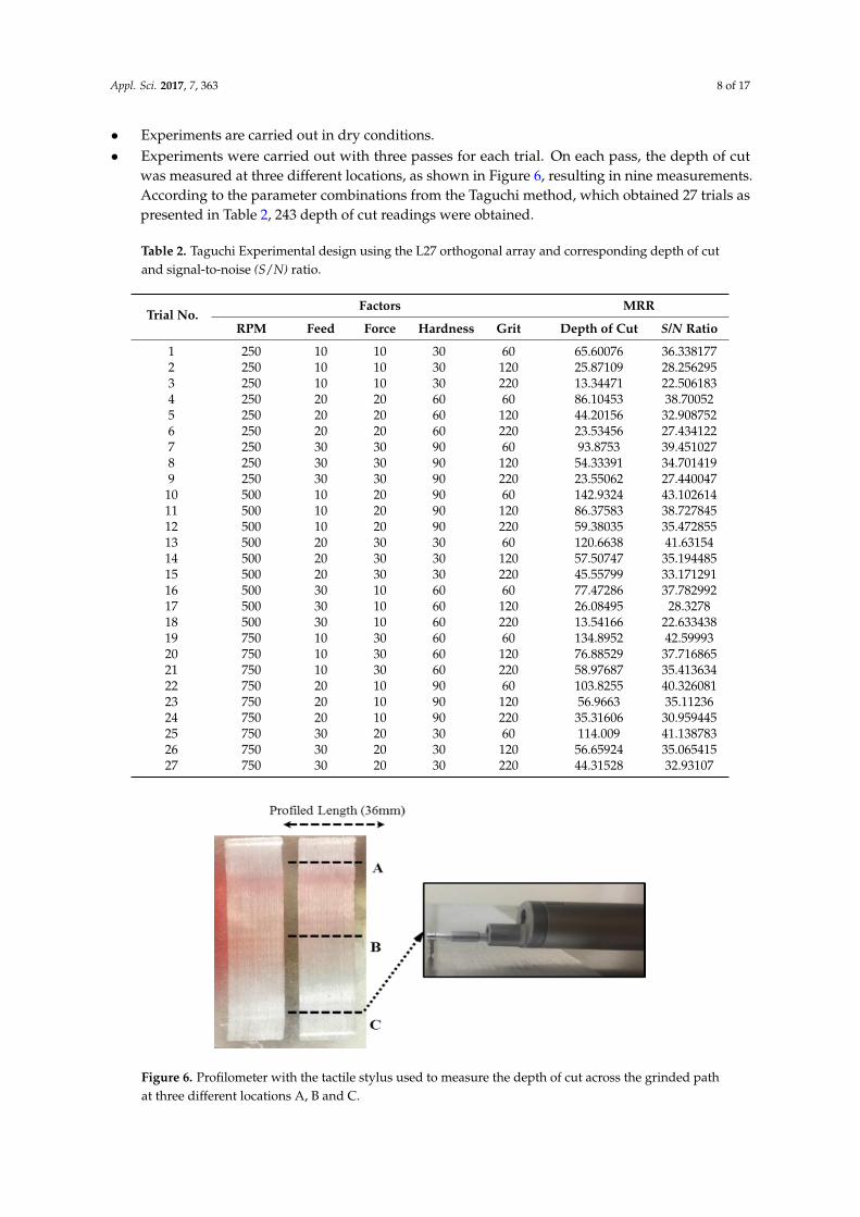
Table 2. Taguchi Experimental design using the L27 orthogonal array and corresponding depth of cutand signal-to-noise (S/N) ratio.

Trial No.Factors MRR

RPM Feed Force Hardness Grit Depth of Cut S/N Ratio

1 250 10 10 30 60 65.60076 36.3381772 250 10 10 30 120 25.87109 28.2562953 250 10 10 30 220 13.34471 22.5061834 250 20 20 60 60 86.10453 38.700525 250 20 20 60 120 44.20156 32.9087526 250 20 20 60 220 23.53456 27.4341227 250 30 30 90 60 93.8753 39.4510278 250 30 30 90 120 54.33391 34.7014199 250 30 30 90 220 23.55062 27.44004710 500 10 20 90 60 142.9324 43.10261411 500 10 20 90 120 86.37583 38.72784512 500 10 20 90 220 59.38035 35.47285513 500 20 30 30 60 120.6638 41.6315414 500 20 30 30 120 57.50747 35.19448515 500 20 30 30 220 45.55799 33.17129116 500 30 10 60 60 77.47286 37.78299217 500 30 10 60 120 26.08495 28.327818 500 30 10 60 220 13.54166 22.63343819 750 10 30 60 60 134.8952 42.5999320 750 10 30 60 120 76.88529 37.71686521 750 10 30 60 220 58.97687 35.41363422 750 20 10 90 60 103.8255 40.32608123 750 20 10 90 120 56.9663 35.1123624 750 20 10 90 220 35.31606 30.95944525 750 30 20 30 60 114.009 41.13878326 750 30 20 30 120 56.65924 35.06541527 750 30 20 30 220 44.31528 32.93107

Appl. Sci. 2017, 7, 363 8 of 17

Figure 6. Profilometer with the tactile stylus used to measure the depth of cut across the grinded path

at three different locations A, B and C.

Table 2. Taguchi Experimental design using the L27 orthogonal array and corresponding depth of

cut and signal-to-noise (S/N) ratio.

Trial No. Factors MRR

RPM Feed Force Hardness Grit Depth of Cut S/N Ratio

1 250 10 10 30 60 65.60076 36.338177

2 250 10 10 30 120 25.87109 28.256295

3 250 10 10 30 220 13.34471 22.506183

4 250 20 20 60 60 86.10453 38.70052

5 250 20 20 60 120 44.20156 32.908752

6 250 20 20 60 220 23.53456 27.434122

7 250 30 30 90 60 93.8753 39.451027

8 250 30 30 90 120 54.33391 34.701419

9 250 30 30 90 220 23.55062 27.440047

10 500 10 20 90 60 142.9324 43.102614

11 500 10 20 90 120 86.37583 38.727845

12 500 10 20 90 220 59.38035 35.472855

13 500 20 30 30 60 120.6638 41.63154

14 500 20 30 30 120 57.50747 35.194485

15 500 20 30 30 220 45.55799 33.171291

16 500 30 10 60 60 77.47286 37.782992

17 500 30 10 60 120 26.08495 28.3278

18 500 30 10 60 220 13.54166 22.633438

19 750 10 30 60 60 134.8952 42.59993

20 750 10 30 60 120 76.88529 37.716865

21 750 10 30 60 220 58.97687 35.413634

22 750 20 10 90 60 103.8255 40.326081

23 750 20 10 90 120 56.9663 35.11236

24 750 20 10 90 220 35.31606 30.959445

25 750 30 20 30 60 114.009 41.138783

26 750 30 20 30 120 56.65924 35.065415

27 750 30 20 30 220 44.31528 32.93107

3.3. Prediction of Depth of Cut

A Mitutoyo stylus profilometer with a stylus tip radius of 5 µm was used to measure the depth

of cut across the grinded path. Mitutoyo profilometer primarily consists of a traverse unit and a

Figure 6. Profilometer with the tactile stylus used to measure the depth of cut across the grinded pathat three different locations A, B and C.

Appl. Sci. 2017, 7, 363 9 of 17

3.3. Prediction of Depth of Cut

A Mitutoyo stylus profilometer with a stylus tip radius of 5 µm was used to measure the depth ofcut across the grinded path. Mitutoyo profilometer primarily consists of a traverse unit and a processorcontrol module. The grinded workpieces are so adjusted that the area of interest of measurement isacross the grinded path. The length is profiled across locations A, B, and C along the tool path, asshown in Figure 6. 3D and 2D profiles were extracted from the workpiece surface across the machinedlength, using the profilometer to measure the depth of cut, as illustrated in Figure 7.

Appl. Sci. 2017, 7, 363 9 of 17

processor control module. The grinded workpieces are so adjusted that the area of interest of

measurement is across the grinded path. The length is profiled across locations A, B, and C along the

tool path, as shown in Figure 6. 3D and 2D profiles were extracted from the workpiece surface across

the machined length, using the profilometer to measure the depth of cut, as illustrated in Figure 7.

The depth of cut is measured as the distance between the deepest point in the grinded path and

the surface of the word coupon. Each experimental trial was repeated three times to have consistency,

and depth of cut was measured across three locations for each trial, resulting in a total of nine reading

per test. Figure 8 shows the standard deviation of the depth of cut measure taken from Taguchi’s L27

orthogonal array based experimental trials for all 27 test conditions. Table 2 shows the experimental

results for the mean depth of cut and corresponding S/N ratios. The depth of cut, i.e., material removal,

was identified as the process output as well as the quality characteristic with the concept ‘the larger-

the-better’. The S/N ratio for the larger-the-better is: S/N = −10 × log (mean square deviation):

𝑆

𝑁= −10𝑙𝑜𝑔10 (

1

𝑛∑

1

𝑦2) (8)

where n is the number of measurements in a trial/row, in this case, n = 1, and y is the measured value

in a run/row. A higher S/N value agrees with a higher depth of cut. Consequently, the ideal level of

the grinding parameters is the level with the most significant S/N value.

Figure 7. (a) 3D profile extracted from the workpiece surface across the machined surface using

Taly-scan; (b) 2D profile obtained from the workpiece surface across the grinded path to measure the

depth of cut.

Figure 7. (a) 3D profile extracted from the workpiece surface across the machined surface usingTaly-scan; (b) 2D profile obtained from the workpiece surface across the grinded path to measure thedepth of cut.

The depth of cut is measured as the distance between the deepest point in the grinded path andthe surface of the word coupon. Each experimental trial was repeated three times to have consistency,and depth of cut was measured across three locations for each trial, resulting in a total of nine readingper test. Figure 8 shows the standard deviation of the depth of cut measure taken from Taguchi’s L27orthogonal array based experimental trials for all 27 test conditions. Table 2 shows the experimentalresults for the mean depth of cut and corresponding S/N ratios. The depth of cut, i.e., materialremoval, was identified as the process output as well as the quality characteristic with the concept ‘thelarger-the-better’. The S/N ratio for the larger-the-better is: S/N = −10 × log (mean square deviation):

SN

= −10log10

(1n ∑

1y2

)(8)

Appl. Sci. 2017, 7, 363 10 of 17

where n is the number of measurements in a trial/row, in this case, n = 1, and y is the measured valuein a run/row. A higher S/N value agrees with a higher depth of cut. Consequently, the ideal level ofthe grinding parameters is the level with the most significant S/N value.Appl. Sci. 2017, 7, 363 10 of 17

Figure 8. Standard deviation of the depth of cut taken from Taguchi based L27 orthogonal

experimental trials.

4. Results and Analysis

Figure 9 presents the results of the S/N ratio for the five parameters at three levels. According to

Figure 9, the optimal parameters for a higher material removal rate were obtained at 750 RPM

(level 3), 10 mm/s feed rate (level 1), 30 N force (level 3), 90 Shore A hardness (level 3), and 60 grit

(level 1). The Material Removal Rate (MRR) increases with increasing Rotation per Minute (RPM),

force, and hardness. On the contrary, it increases with decreasing feed and grit size. With coarser

grain, i.e., smaller grit size, the depth of cut increases. An increase in force imparted on the work

coupon and hardness of contact wheel results in an increase of material removal. The increase of RPM

in the contact wheel causes greater tangential force, thereby causing the enhancement of the depth of

cut. The decrease in feed rate causes the contact time between the grains and work coupon to be

maximized, resulting in a higher material removal rate.

Figure 9. Mean signal-to-noise (S/N) ratio graph for depth of cut.

Figure 8. Standard deviation of the depth of cut taken from Taguchi based L27 orthogonal experimental trials.

4. Results and Analysis

Figure 9 presents the results of the S/N ratio for the five parameters at three levels. Accordingto Figure 9, the optimal parameters for a higher material removal rate were obtained at 750 RPM(level 3), 10 mm/s feed rate (level 1), 30 N force (level 3), 90 Shore A hardness (level 3), and 60 grit(level 1). The Material Removal Rate (MRR) increases with increasing Rotation per Minute (RPM),force, and hardness. On the contrary, it increases with decreasing feed and grit size. With coarsergrain, i.e., smaller grit size, the depth of cut increases. An increase in force imparted on the workcoupon and hardness of contact wheel results in an increase of material removal. The increase of RPMin the contact wheel causes greater tangential force, thereby causing the enhancement of the depthof cut. The decrease in feed rate causes the contact time between the grains and work coupon to bemaximized, resulting in a higher material removal rate.

Appl. Sci. 2017, 7, 363 10 of 17

Figure 8. Standard deviation of the depth of cut taken from Taguchi based L27 orthogonal

experimental trials.

4. Results and Analysis

Figure 9 presents the results of the S/N ratio for the five parameters at three levels. According to

Figure 9, the optimal parameters for a higher material removal rate were obtained at 750 RPM

(level 3), 10 mm/s feed rate (level 1), 30 N force (level 3), 90 Shore A hardness (level 3), and 60 grit

(level 1). The Material Removal Rate (MRR) increases with increasing Rotation per Minute (RPM),

force, and hardness. On the contrary, it increases with decreasing feed and grit size. With coarser

grain, i.e., smaller grit size, the depth of cut increases. An increase in force imparted on the work

coupon and hardness of contact wheel results in an increase of material removal. The increase of RPM

in the contact wheel causes greater tangential force, thereby causing the enhancement of the depth of

cut. The decrease in feed rate causes the contact time between the grains and work coupon to be

maximized, resulting in a higher material removal rate.

Figure 9. Mean signal-to-noise (S/N) ratio graph for depth of cut.

Figure 9. Mean signal-to-noise (S/N) ratio graph for depth of cut.

Appl. Sci. 2017, 7, 363 11 of 17

4.1. Analysis of Variance (ANOVA)

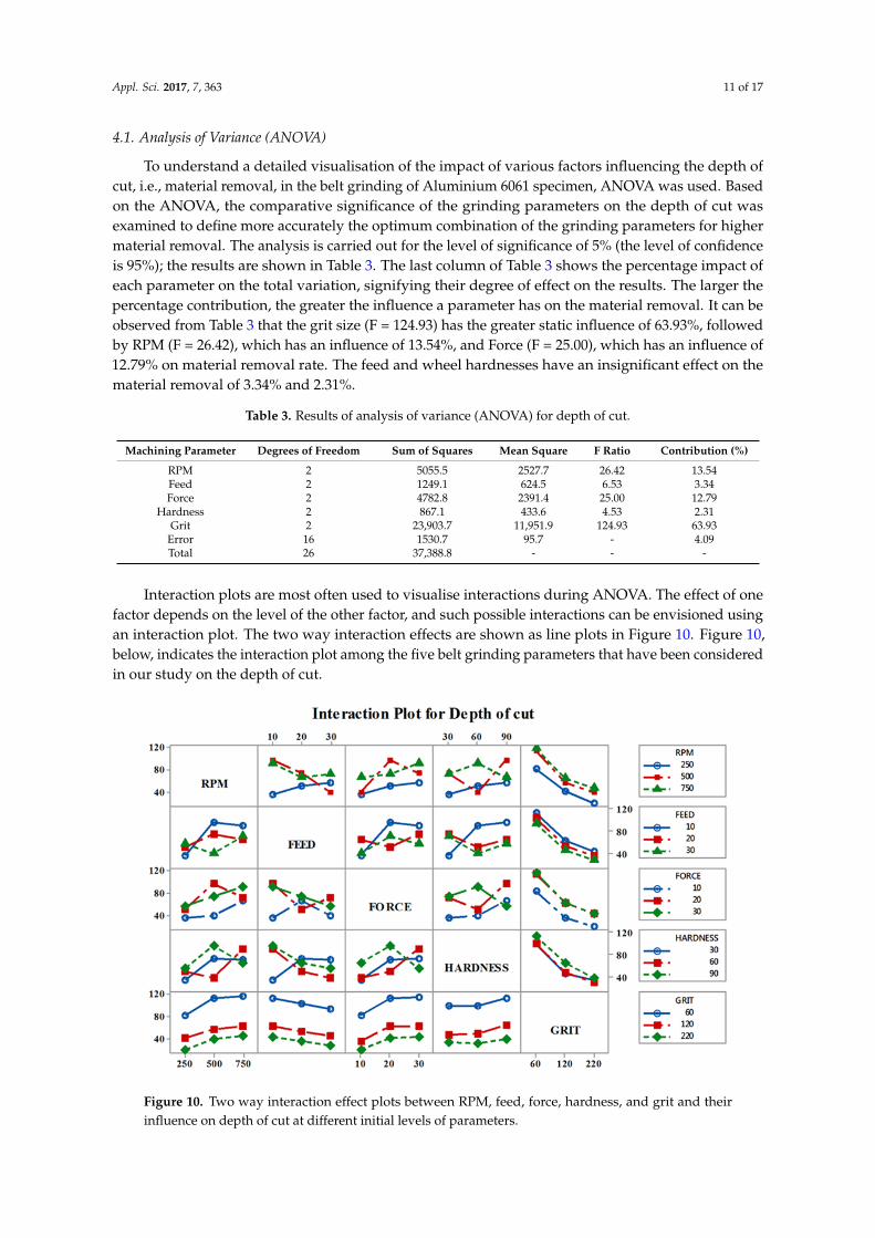
To understand a detailed visualisation of the impact of various factors influencing the depth ofcut, i.e., material removal, in the belt grinding of Aluminium 6061 specimen, ANOVA was used. Basedon the ANOVA, the comparative significance of the grinding parameters on the depth of cut wasexamined to define more accurately the optimum combination of the grinding parameters for highermaterial removal. The analysis is carried out for the level of significance of 5% (the level of confidenceis 95%); the results are shown in Table 3. The last column of Table 3 shows the percentage impact ofeach parameter on the total variation, signifying their degree of effect on the results. The larger thepercentage contribution, the greater the influence a parameter has on the material removal. It can beobserved from Table 3 that the grit size (F = 124.93) has the greater static influence of 63.93%, followedby RPM (F = 26.42), which has an influence of 13.54%, and Force (F = 25.00), which has an influence of12.79% on material removal rate. The feed and wheel hardnesses have an insignificant effect on thematerial removal of 3.34% and 2.31%.

Table 3. Results of analysis of variance (ANOVA) for depth of cut.

Machining Parameter Degrees of Freedom Sum of Squares Mean Square F Ratio Contribution (%)

RPM 2 5055.5 2527.7 26.42 13.54Feed 2 1249.1 624.5 6.53 3.34Force 2 4782.8 2391.4 25.00 12.79

Hardness 2 867.1 433.6 4.53 2.31Grit 2 23,903.7 11,951.9 124.93 63.93

Error 16 1530.7 95.7 - 4.09Total 26 37,388.8 - - -

Interaction plots are most often used to visualise interactions during ANOVA. The effect of onefactor depends on the level of the other factor, and such possible interactions can be envisioned usingan interaction plot. The two way interaction effects are shown as line plots in Figure 10. Figure 10,below, indicates the interaction plot among the five belt grinding parameters that have been consideredin our study on the depth of cut.

Appl. Sci. 2017, 7, 363 11 of 17

4.1. Analysis of Variance (ANOVA)

To understand a detailed visualisation of the impact of various factors influencing the depth of

cut, i.e., material removal, in the belt grinding of Aluminium 6061 specimen, ANOVA was used.

Based on the ANOVA, the comparative significance of the grinding parameters on the depth of cut

was examined to define more accurately the optimum combination of the grinding parameters for

higher material removal. The analysis is carried out for the level of significance of 5% (the level of

confidence is 95%); the results are shown in Table 3. The last column of Table 3 shows the percentage

impact of each parameter on the total variation, signifying their degree of effect on the results.

The larger the percentage contribution, the greater the influence a parameter has on the material

removal. It can be observed from Table 3 that the grit size (F = 124.93) has the greater static influence

of 63.93%, followed by RPM (F = 26.42), which has an influence of 13.54%, and Force (F = 25.00), which has

an influence of 12.79% on material removal rate. The feed and wheel hardnesses have an insignificant

effect on the material removal of 3.34% and 2.31%.

Table 3. Results of analysis of variance (ANOVA) for depth of cut.

Machining Parameter Degrees of Freedom Sum of Squares Mean Square F Ratio Contribution (%)

RPM 2 5055.5 2527.7 26.42 13.54

Feed 2 1249.1 624.5 6.53 3.34

Force 2 4782.8 2391.4 25.00 12.79

Hardness 2 867.1 433.6 4.53 2.31

Grit 2 23,903.7 11,951.9 124.93 63.93

Error 16 1530.7 95.7 - 4.09

Total 26 37,388.8 - - -

Interaction plots are most often used to visualise interactions during ANOVA. The effect of one

factor depends on the level of the other factor, and such possible interactions can be envisioned using

an interaction plot. The two way interaction effects are shown as line plots in Figure 10. Figure 10,

below, indicates the interaction plot among the five belt grinding parameters that have been

considered in our study on the depth of cut.

Figure 10. Two way interaction effect plots between RPM, feed, force, hardness, and grit and their

influence on depth of cut at different initial levels of parameters. Figure 10. Two way interaction effect plots between RPM, feed, force, hardness, and grit and theirinfluence on depth of cut at different initial levels of parameters.

Appl. Sci. 2017, 7, 363 12 of 17

4.2. Predictive Modelling of Material Removal Using ANFIS

Adaptive neuro-fuzzy inference system (ANFIS) removes the primary problem in fuzzy if-thenrules by using the learning ability of an artificial neural network (ANN) for automated tuning of fuzzyif-then rules during training, resulting in a change of the membership function of parameters, thusleading to the automatic adaptation of the fuzzy system based on inputs-output space. The initial stepof the ANFIS modelling system is to decide the input and output variables of the fuzzy logic controller.The ANFIS model described in this paper has five input parameters; RPM, feed, force, hardness, grit,and the output as the depth of cut, i.e., material removal rate (MRR).

The ANFIS model described in this paper is a Multiple Input Single Output (MISO) system withmultiple inputs and a single output. Figure 11 shows real inputs and real output with fuzzy rulearchitecture of the ANFIS. A Taguchi based experimental design with 27 runs, as indicated in Table 2,is used as the inputs for the ANFIS model.

Appl. Sci. 2017, 7, 363 12 of 17

4.2. Predictive Modelling of Material Removal Using ANFIS

Adaptive neuro-fuzzy inference system (ANFIS) removes the primary problem in fuzzy if-then

rules by using the learning ability of an artificial neural network (ANN) for automated tuning of

fuzzy if-then rules during training, resulting in a change of the membership function of parameters,

thus leading to the automatic adaptation of the fuzzy system based on inputs-output space. The initial

step of the ANFIS modelling system is to decide the input and output variables of the fuzzy logic

controller. The ANFIS model described in this paper has five input parameters; RPM, feed, force,

hardness, grit, and the output as the depth of cut, i.e., material removal rate (MRR).

The ANFIS model described in this paper is a Multiple Input Single Output (MISO) system with

multiple inputs and a single output. Figure 11 shows real inputs and real output with fuzzy rule

architecture of the ANFIS. A Taguchi based experimental design with 27 runs, as indicated in Table 2,

is used as the inputs for the ANFIS model.

Figure 11. Adaptive Neuro-Fuzzy Inference System (ANFIS) model for belt grinding showing

inputs and output.

4.2.1. Membership Functions for the Input and Output Variables

A membership function allocates grades of membership extending from numbers between zero

and one to the range of the possible values of the variable. Zero membership value specifies that it is

not a member of the fuzzy-set; one signifies an extensive member. A membership function such as

sigmoidal membership function is created for each input variable used in belt grinding, as illustrated

in Figure 11. The sigmoid function is differentiable for all values of the inputs to allow the use of

powerful back-propagation learning algorithms [20]. The application of general sigmoidal

membership functions to the neuro-fuzzy modelling process is a very attractive methodology to

characterise nonlinear processes [21]. The advantage of sigmoidal membership functions over other

membership functions is the better approximation due to tapering edges.

4.2.2. ANFIS Rules Employed in Model

The fuzzy modelling of Abrasive Belt Grinding uses five input parameters and one output

parameter. The five input parameters include cutting speed, shore A hardness, feed, force, and grit

size, and the output parameter is the material depth of cut. Each parameter corresponds to six

linguistic variables. These variables can generate a number of rules in the designed control rules of

the system. The topology of ANFIS architecture that implements the sigmoidal membership function

Figure 11. Adaptive Neuro-Fuzzy Inference System (ANFIS) model for belt grinding showing inputsand output.

4.2.1. Membership Functions for the Input and Output Variables

A membership function allocates grades of membership extending from numbers between zeroand one to the range of the possible values of the variable. Zero membership value specifies that it isnot a member of the fuzzy-set; one signifies an extensive member. A membership function such assigmoidal membership function is created for each input variable used in belt grinding, as illustratedin Figure 11. The sigmoid function is differentiable for all values of the inputs to allow the use ofpowerful back-propagation learning algorithms [20]. The application of general sigmoidal membershipfunctions to the neuro-fuzzy modelling process is a very attractive methodology to characterisenonlinear processes [21]. The advantage of sigmoidal membership functions over other membershipfunctions is the better approximation due to tapering edges.

4.2.2. ANFIS Rules Employed in Model

The fuzzy modelling of Abrasive Belt Grinding uses five input parameters and one outputparameter. The five input parameters include cutting speed, shore A hardness, feed, force, and

Appl. Sci. 2017, 7, 363 13 of 17

grit size, and the output parameter is the material depth of cut. Each parameter corresponds to sixlinguistic variables. These variables can generate a number of rules in the designed control rules ofthe system. The topology of ANFIS architecture that implements the sigmoidal membership functiondesigned with 243 fuzzy rules for depth of cut prediction used in this research is illustrated inFigure 12. Figure 12 present an ANFIS architecture that is equivalent to a five-input first-order Sugenofuzzy model. The ANFIS used contains 243 rules, with sigmoidal membership functions assigned toeach input variable. The total number of fitting parameters is 303, including 60 premise (nonlinear)parameters and 243 consequent (linear) parameters. The applicable control rules formulated alongwith the membership function for the model are shown in rule viewer of the fuzzy model, as presentedin Figure 13. These rules were implemented in a MATLAB environment using a Sugeno-type fuzzyinference system in the fuzzy logic toolbox.

Appl. Sci. 2017, 7, 363 13 of 17

designed with 243 fuzzy rules for depth of cut prediction used in this research is illustrated in Figure 12.

Figure 12 present an ANFIS architecture that is equivalent to a five-input first-order Sugeno fuzzy

model. The ANFIS used contains 243 rules, with sigmoidal membership functions assigned to each

input variable. The total number of fitting parameters is 303, including 60 premise (nonlinear)

parameters and 243 consequent (linear) parameters. The applicable control rules formulated along

with the membership function for the model are shown in rule viewer of the fuzzy model, as presented

in Figure 13. These rules were implemented in a MATLAB environment using a Sugeno-type fuzzy

inference system in the fuzzy logic toolbox.

Figure 12. Topology of adaptive neuro-fuzzy inference system architecture.

Figure 13. A part of the rule viewer in the proposed fuzzy model.

Figure 14 presents the initial and final membership functions of the five belt grinding input

parameters derived by sigmoidal membership function training. It can be seen from Figure 14 that

Figure 12. Topology of adaptive neuro-fuzzy inference system architecture.

Appl. Sci. 2017, 7, 363 13 of 17

designed with 243 fuzzy rules for depth of cut prediction used in this research is illustrated in Figure 12.

Figure 12 present an ANFIS architecture that is equivalent to a five-input first-order Sugeno fuzzy

model. The ANFIS used contains 243 rules, with sigmoidal membership functions assigned to each

input variable. The total number of fitting parameters is 303, including 60 premise (nonlinear)

parameters and 243 consequent (linear) parameters. The applicable control rules formulated along

with the membership function for the model are shown in rule viewer of the fuzzy model, as presented

in Figure 13. These rules were implemented in a MATLAB environment using a Sugeno-type fuzzy

inference system in the fuzzy logic toolbox.

Figure 12. Topology of adaptive neuro-fuzzy inference system architecture.

Figure 13. A part of the rule viewer in the proposed fuzzy model.

Figure 14 presents the initial and final membership functions of the five belt grinding input

parameters derived by sigmoidal membership function training. It can be seen from Figure 14 that

Figure 13. A part of the rule viewer in the proposed fuzzy model.

Appl. Sci. 2017, 7, 363 14 of 17

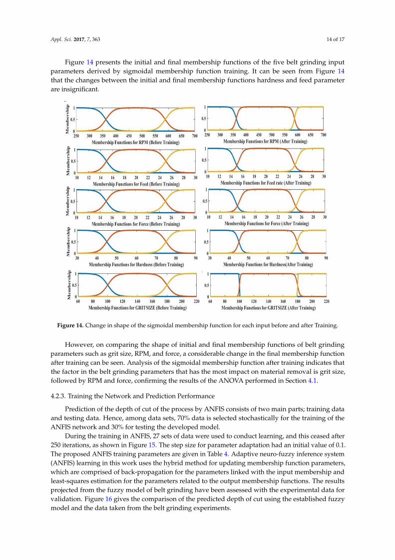
Figure 14 presents the initial and final membership functions of the five belt grinding inputparameters derived by sigmoidal membership function training. It can be seen from Figure 14that the changes between the initial and final membership functions hardness and feed parameterare insignificant.

Appl. Sci. 2017, 7, 363 14 of 17

the changes between the initial and final membership functions hardness and feed parameter are

insignificant.

Figure 14. Change in shape of the sigmoidal membership function for each input before and

after Training.

However, on comparing the shape of initial and final membership functions of belt grinding

parameters such as grit size, RPM, and force, a considerable change in the final membership function

after training can be seen. Analysis of the sigmoidal membership function after training indicates that

the factor in the belt grinding parameters that has the most impact on material removal is grit size,

followed by RPM and force, confirming the results of the ANOVA performed in Section 4.1.

4.2.3. Training the Network and Prediction Performance

Prediction of the depth of cut of the process by ANFIS consists of two main parts; training data

and testing data. Hence, among data sets, 70% data is selected stochastically for the training of the

ANFIS network and 30% for testing the developed model.

During the training in ANFIS, 27 sets of data were used to conduct learning, and this ceased

after 250 iterations, as shown in Figure 15. The step size for parameter adaptation had an initial value

of 0.1. The proposed ANFIS training parameters are given in Table 4. Adaptive neuro-fuzzy inference

system (ANFIS) learning in this work uses the hybrid method for updating membership function

parameters, which are comprised of back-propagation for the parameters linked with the input

membership and least-squares estimation for the parameters related to the output membership

functions. The results projected from the fuzzy model of belt grinding have been assessed with the

experimental data for validation. Figure 16 gives the comparison of the predicted depth of cut using

the established fuzzy model and the data taken from the belt grinding experiments.

Figure 14. Change in shape of the sigmoidal membership function for each input before and after Training.

However, on comparing the shape of initial and final membership functions of belt grindingparameters such as grit size, RPM, and force, a considerable change in the final membership functionafter training can be seen. Analysis of the sigmoidal membership function after training indicates thatthe factor in the belt grinding parameters that has the most impact on material removal is grit size,followed by RPM and force, confirming the results of the ANOVA performed in Section 4.1.

4.2.3. Training the Network and Prediction Performance

Prediction of the depth of cut of the process by ANFIS consists of two main parts; training dataand testing data. Hence, among data sets, 70% data is selected stochastically for the training of theANFIS network and 30% for testing the developed model.

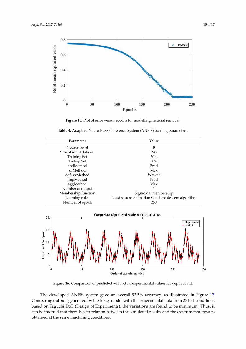
During the training in ANFIS, 27 sets of data were used to conduct learning, and this ceased after250 iterations, as shown in Figure 15. The step size for parameter adaptation had an initial value of 0.1.The proposed ANFIS training parameters are given in Table 4. Adaptive neuro-fuzzy inference system(ANFIS) learning in this work uses the hybrid method for updating membership function parameters,which are comprised of back-propagation for the parameters linked with the input membership andleast-squares estimation for the parameters related to the output membership functions. The resultsprojected from the fuzzy model of belt grinding have been assessed with the experimental data forvalidation. Figure 16 gives the comparison of the predicted depth of cut using the established fuzzymodel and the data taken from the belt grinding experiments.

Appl. Sci. 2017, 7, 363 15 of 17

Appl. Sci. 2017, 7, 363 15 of 17

Table 4. Adaptive Neuro-Fuzzy Inference System (ANFIS) training parameters.

Parameter Value

Neuron level 5

Size of input data set 243

Training Set 70%

Testing Set 30%

andMethod Prod

orMethod Max

defuzzMethod Wtaver

impMethod Prod

aggMethod Max

Number of output 1

Membership function Sigmoidal membership

Learning rules Least square estimation-Gradient descent algorithm

Number of epoch 250

Figure 15. Plot of error versus epochs for modelling material removal.

Figure 16. Comparison of predicted with actual experimental values for depth of cut.

The developed ANFIS system gave an overall 93.5% accuracy, as illustrated in Figure 17.

Comparing outputs generated by the fuzzy model with the experimental data from 27 test conditions

based on Taguchi DoE (Design of Experiments), the variations are found to be minimum. Thus, it can

Figure 15. Plot of error versus epochs for modelling material removal.

Table 4. Adaptive Neuro-Fuzzy Inference System (ANFIS) training parameters.

Parameter Value

Neuron level 5Size of input data set 243

Training Set 70%Testing Set 30%andMethod ProdorMethod Max

defuzzMethod WtaverimpMethod ProdaggMethod Max

Number of output 1Membership function Sigmoidal membership

Learning rules Least square estimation-Gradient descent algorithmNumber of epoch 250

Appl. Sci. 2017, 7, 363 15 of 17

Table 4. Adaptive Neuro-Fuzzy Inference System (ANFIS) training parameters.

Parameter Value

Neuron level 5

Size of input data set 243

Training Set 70%

Testing Set 30%

andMethod Prod

orMethod Max

defuzzMethod Wtaver

impMethod Prod

aggMethod Max

Number of output 1

Membership function Sigmoidal membership

Learning rules Least square estimation-Gradient descent algorithm

Number of epoch 250

Figure 15. Plot of error versus epochs for modelling material removal.

Figure 16. Comparison of predicted with actual experimental values for depth of cut.

The developed ANFIS system gave an overall 93.5% accuracy, as illustrated in Figure 17.

Comparing outputs generated by the fuzzy model with the experimental data from 27 test conditions

based on Taguchi DoE (Design of Experiments), the variations are found to be minimum. Thus, it can

Figure 16. Comparison of predicted with actual experimental values for depth of cut.

The developed ANFIS system gave an overall 93.5% accuracy, as illustrated in Figure 17.Comparing outputs generated by the fuzzy model with the experimental data from 27 test conditionsbased on Taguchi DoE (Design of Experiments), the variations are found to be minimum. Thus, itcan be inferred that there is a co-relation between the simulated results and the experimental resultsobtained at the same machining conditions.

Appl. Sci. 2017, 7, 363 16 of 17

Appl. Sci. 2017, 7, 363 16 of 17

be inferred that there is a co-relation between the simulated results and the experimental results

obtained at the same machining conditions.

Figure 17. Correlation between actual and predicted values of test and train data set.

5. Conclusions

In this study, an investigation into the influence of belt grinding parameters on material removal

depth based on the Taguchi parameter design method has been analysed and presented. In the belt

grinding experiments, three levels of cutting wheel speed, feed rate, force, grit size, and polymer

hardness were applied. Based on the experimental results and summarising the research, the following

generalised conclusions are drawn:

1. ANOVA determined the level of significance of the machining parameters on the material depth

of cut. Based on the analysis of variance (ANOVA) results at a 95% confidence level, the highly

dominant parameters of material removal are identified. Namely, the grit size grinding

parameter is the primary factor that has the highest influence on the material removal, and this

parameter is about five times greater than the second ranking parameters (RPM and force

imparted). The feed rate and polymer wheel hardness parameters do not seem to have much of

an influence on the depth of cut, i.e., material removal. Results from ANOVA interactions also

suggests that the experimental trials can further be optimised using Taguchi Interaction instead

of orthogonal design.

2. Based on the signal-to-noise ratio results in Figure 9, we can construe that 750 RPM, 10 mm/s

feed rate, 30 N force, 90 Shore A hardness, and 60 grit size are the optimal grinding parameters

for achieving maximum depth of cut.

3. A method of modelling and calculating the material removal using ANFIS is proposed in this

paper. The ANFIS model developed is validated with experimental trials for given conditions.

It has been identified that results produced by the designed regression model have acceptable

deviations between the predicted and the actual experimental results with 93.5% accuracy. The

ANFIS model developed in this research work is viable and could be used to predict the depth

of cut, i.e., material removal for an Abrasive Belt Grinding process.

Acknowledgments: This work was conducted within the Rolls-Royce@NTU Corporate Lab with support from

the National Research Foundation (NRF), Singapore, under the Corp Lab@University Scheme.

Figure 17. Correlation between actual and predicted values of test and train data set.

5. Conclusions

In this study, an investigation into the influence of belt grinding parameters on material removaldepth based on the Taguchi parameter design method has been analysed and presented. In the beltgrinding experiments, three levels of cutting wheel speed, feed rate, force, grit size, and polymerhardness were applied. Based on the experimental results and summarising the research, the followinggeneralised conclusions are drawn:

1. ANOVA determined the level of significance of the machining parameters on the materialdepth of cut. Based on the analysis of variance (ANOVA) results at a 95% confidence level, thehighly dominant parameters of material removal are identified. Namely, the grit size grindingparameter is the primary factor that has the highest influence on the material removal, andthis parameter is about five times greater than the second ranking parameters (RPM and forceimparted). The feed rate and polymer wheel hardness parameters do not seem to have much ofan influence on the depth of cut, i.e., material removal. Results from ANOVA interactions alsosuggests that the experimental trials can further be optimised using Taguchi Interaction insteadof orthogonal design.

2. Based on the signal-to-noise ratio results in Figure 9, we can construe that 750 RPM, 10 mm/sfeed rate, 30 N force, 90 Shore A hardness, and 60 grit size are the optimal grinding parametersfor achieving maximum depth of cut.

3. A method of modelling and calculating the material removal using ANFIS is proposed in thispaper. The ANFIS model developed is validated with experimental trials for given conditions.It has been identified that results produced by the designed regression model have acceptabledeviations between the predicted and the actual experimental results with 93.5% accuracy. TheANFIS model developed in this research work is viable and could be used to predict the depth ofcut, i.e., material removal for an Abrasive Belt Grinding process.

Acknowledgments: This work was conducted within the Rolls-Royce@NTU Corporate Lab with support fromthe National Research Foundation (NRF), Singapore, under the Corp Lab@University Scheme.

Author Contributions: Vigneashwara Pandiyan conducted Data curation, investigation, data processing, formalanalysis and original draft preparation. Wahyu Caesarendra conducted data processing, formal analysis,

Appl. Sci. 2017, 7, 363 17 of 17

validation, review and editing. Tegoeh Tjahjowidodo provided Funding acquisition, conceptualization, resources,formal analysis, review and editing. Gunasekaran Praveen conducted Data curation and original draft preparation.

Conflicts of Interest: The authors declare no conflict of interest.

References

1. Zhang, X.; Kuhlenkötter, B.; Kneupner, K. An efficient method for solving the Signorini problem in thesimulation of free-form surfaces produced by belt grinding. Int. J. Mach. Tools Manuf. 2005, 45, 641–648.[CrossRef]

2. Jourani, A.; Dursapt, M.; Hamdi, H.; Rech, J.; Zahouani, H. Effect of the belt grinding on the surface texture:Modeling of the contact and abrasive wear. Wear 2005, 259, 1137–1143. [CrossRef]

3. Ren, X.; Cabaravdic, M.; Zhang, X.; Kuhlenkötter, B. A local process model for simulation of robotic beltgrinding. Int. J. Mach. Tools Manuf. 2007, 47, 962–970. [CrossRef]

4. Ren, X.; Kuhlenkötter, B.; Müller, H. Simulation and verification of belt grinding with industrial robots. Int. J.Mach. Tools Manuf. 2006, 46, 708–716. [CrossRef]

5. Hamann, G. Modellierung des Abtragsverhaltens Elastischer Robotergefuehrter Schleifwerkzeuge; University ofStuttgart: Stuttgart, Germany, 1998.

6. Rufeng, X.; Chen, Z.; Chen, W.; Wu, X.; Zhu, J. Dual drive curve tool path planning method for 5-axis NCmachining of sculptured surfaces. Chin. J. Aeronaut. 2010, 23, 486–494. [CrossRef]

7. Zhang, X.; Kneupner, K.; Kuhlenkötter, B. A new force distribution calculation model for high-qualityproduction processes. Int. J. Adv. Manuf. Technol. 2006, 27, 726–732. [CrossRef]

8. Radzevich, S.P. A closed-form solution to the problem of optimal tool-path generation for sculptured surfacemachining on multi-axis NC machine. Math. Comput. Model. 2006, 43, 222–243. [CrossRef]

9. Pi, J.; Red, E.; Jensen, G. Grind-free tool path generation for five-axis surface machining. Comput. Integr.Manuf. Syst. 1998, 11, 337–350. [CrossRef]

10. Taguchi, G. Introduction to Quality Engineering: Designing Quality into Products and Processes; AsianProducativity Organization: Tokyo, Japan, 1986.

11. Lindman, H.R. Analysis of Variance in Experimental Design; Springer Science & Business Media: New York,NY, USA, 2012.

12. Gill, S.S.; Singh, J. An Adaptive Neuro-Fuzzy Inference System modeling for material removal rate instationary ultrasonic drilling of sillimanite ceramic. Expert Syst. Appl. 2010, 37, 5590–5598. [CrossRef]

13. Çaydas, U.; Hasçalık, A.; Ekici, S. An adaptive neuro-fuzzy inference system (ANFIS) model for wire-EDM.Expert Syst. Appl. 2009, 36, 6135–6139. [CrossRef]

14. Jang, J.-S.R. ANFIS: Adaptive-network-based fuzzy inference system. IEEE Trans. Syst. Man Cybern. 1993, 23,665–685. [CrossRef]

15. Wang, S.; Li, C. Application and development of high-efficiency abrasive process. Int. J. Adv. Manuf. Technol.2012, 47, 51–64.

16. Huang, H.; Gong, Z.M.; Chen, X.Q.; Zhou, L. Robotic grinding and polishing for turbine-vane overhaul.J. Mater. Process. Technol. 2002, 127, 140–145. [CrossRef]

17. Lei, Y.; He, Z.; Zi, Y. A new approach to intelligent fault diagnosis of rotating machinery. Expert Syst. Appl.2008, 35, 1593–1600. [CrossRef]

18. Ying, L.-C.; Pan, M.-C. Using adaptive network based fuzzy inference system to forecast regional electricityloads. Energy Convers. Manag. 2008, 49, 205–211. [CrossRef]

19. Zadeh, L.A. Fuzzy sets. Inf. Control 1965, 8, 338–353. [CrossRef]20. Werbos, P.J. Backpropagation through time: What it does and how to do it. Proc. IEEE 1990, 78, 1550–1560.

[CrossRef]21. Yilmaz, O.; Bozdana, A.T.; Okka, M.A. An intelligent and automated system for electrical discharge drilling

of aerospace alloys: Inconel 718 and Ti-6Al-4V. Int. J. Adv. Manuf. Technol. 2014, 74, 1323–1336. [CrossRef]

© 2017 by the authors. Licensee MDPI, Basel, Switzerland. This article is an open accessarticle distributed under the terms and conditions of the Creative Commons Attribution(CC BY) license (http://creativecommons.org/licenses/by/4.0/).