Tampereen teknillinen yliopisto. Julkaisu 1190 Tampere University of Technology. Publication 1190

Tapio Manninen Predictive Modeling Using Sparse Logistic Regression with Applications Thesis for the degree of Doctor of Science in Technology to be presented with due permission for public examination and criticism in Tietotalo Building, Auditorium TB109, at Tampere University of Technology, on the 31st of January 2014, at 12 noon. Tampereen teknillinen yliopisto - Tampere University of Technology Tampere 2014

ISBN 978-952-15-3226-9 (printed) ISBN 978-952-15-3233-7 (PDF) ISSN 1459-2045

Abstract

In this thesis, sparse logistic regression models are applied in a set ofreal world machine learning applications. The studied cases includesupervised image segmentation, cancer diagnosis, and MEG data clas-sification. Image segmentation is applied both in component detectionin inkjet printed electronics manufacturing and in cell detection frommicroscope images. The results indicate that a simple linear classifi-cation method such as logistic regression often outperforms more so-phisticated methods. Further, it is shown that the interpretability ofthe linear model offers great advantage in many applications. Modelvalidation and automatic feature selection by means of `1 regularizedparameter estimation have a significant role in this thesis. It is shownthat a combination of a careful model assessment scheme and auto-matic feature selection by means of logistic regression model and coef-ficient regularization create a powerful, yet simple and practical, toolchain for applications of supervised learning and classification.

i

Preface

This work has been carried out at the Department of Signal Process-ing, Tampere University of Technology (TUT), during 2011–2013. Thefunding was provided by Tampere Graduate School in Information Sci-ence and Engineering (TISE). I thank TISE and feel sorry that theyhad to shut the graduate school down. I surely miss those annual cruiseseminars with the good people on board.

I wish to express my sincerest gratitude to my thesis supervisorProf. Ari Visa. Without a doubt, he is the wisest man I have ever met.Whenever was I unsure about the impact of my dissertation for thescientific community, a short discussion with Prof. Visa helped me tocontinue with a perfect reasoning, structure, and logic in my mind.

In addition to Prof. Visa, I’m deeply obliged to thank my closest su-pervisor Heikki Huttunen. There is no question that Heikki is the sin-gle most influential person to my work as well as in gaining any of myacademic achievements. Anyone else being my supervisor and I dareto claim that I would not be writing this preface right now. This claimis based on the simple fact that, to the best of my knowledge, Heikkiis the most committed scientist there is. He always knows what to doand when to do, even in desperate situations. This has also reflectedinto my work via his supervision.

In addition to my supervisors, I’d like to express gratitude to allmy coauthors and all the great people that I have been allowed towork with during the last couple of years. These people include RistoRönkkä, the guy who had enough faith to leave his well establishedposition in a big mobile phone company and start a printed electronicsbusiness with a bunch of tech heads like me. There is also Kalle Ru-tanen, with whom I have always had the most interesting and fruitfuldiscussions (mainly about technical stuff such as geometric transfor-mations) and Pekka Ruusuvuori, the tireless scientist with whom I’mgrateful to have been able to do science as well as to make a coupleof experience gaining conference trips. There are also others than the

ii

people mentioned above and I thank you as well. It must be the posi-tive and encouraging atmosphere at TUT, especially at the Departmentof Signal Processing, that collects all these good people here.

Last but not least, I’d like to let my family and friends know thatyour contribution to whatever I’ve been doing in my chamber for thelast couple of years has been more substantial than you think. I willhappily continue to clear my mom’s laptop from malware and keep ly-ing to my friends about curing the cancer as long as I can keep youin my life as a counter weight for my work. Special thanks goto thepeople in the greatest office band ever, to you Pasi, Frank, and Jenni,for offering me the joy of playing music and having fun with such agood group of people. I’d also like to mention all the great friends that Ihave, especially those made during the year 2013. I’m grateful to Mariawho has introduced me to several magnificent people as well as to theLondon Gang with whom we have had multiple marvelous adventures.The last year has undoubtedly been the best of my life since childhood.That’s because of you.

So, I started as a research assistant in the Department of SignalProcessing in 2007 and was extremely lucky to be able to work throughmy Bachelor’s, Master’s, and PhD, all in a single continuous and logicalsequence while simultaneously working in a series of interesting ma-chine learning projects. Now that I’m finishing my PhD, it seems thatthe time has come for my academic career to come to end and for meto continue my journey in the scary world of industry. If one thing issure, however, you never know what the future brings you.

Tapio ManninenTampere, 2014

iii

Contents

Abstract i

Preface ii

List of Abbreviations vi

Mathematical Notation viii

1 Introduction 11.1 Machine Learning and Pattern Recognition . . . . . . . . 31.2 Introduction to Linear Classification . . . . . . . . . . . . 51.3 Objectives . . . . . . . . . . . . . . . . . . . . . . . . . . . 81.4 Outline . . . . . . . . . . . . . . . . . . . . . . . . . . . . . 91.5 Publications and Author’s Contribution . . . . . . . . . . 10

2 Logistic Regression Classification and Sparse ParameterEstimation 122.1 Background . . . . . . . . . . . . . . . . . . . . . . . . . . 122.2 Logistic Regression Model . . . . . . . . . . . . . . . . . . 132.3 Learning the Model Coefficients . . . . . . . . . . . . . . . 15

2.3.1 Maximum Likelihood Method . . . . . . . . . . . . 152.3.2 Regularization . . . . . . . . . . . . . . . . . . . . . 162.3.3 Bayesian Methods . . . . . . . . . . . . . . . . . . . 19

2.4 Markov Random Field Priors . . . . . . . . . . . . . . . . 23

3 Model Selection and Error Estimation 283.1 Measuring Model Performance . . . . . . . . . . . . . . . 28

3.1.1 Counting Based Performance Measures . . . . . . 293.1.2 Order Based Performance Measures . . . . . . . . 31

3.2 Model Validation and Automatic Parameter Selection . . 333.2.1 Cross-validation . . . . . . . . . . . . . . . . . . . . 34

iv

3.2.2 Bootstrapping . . . . . . . . . . . . . . . . . . . . . 353.2.3 Parametric Methods . . . . . . . . . . . . . . . . . 353.2.4 Pitfalls in Cross-Validation . . . . . . . . . . . . . 383.2.5 The Effect of Sample Size in Error Estimation . . 41

4 Case Studies 444.1 Supervised Image Segmentation . . . . . . . . . . . . . . 44

4.1.1 Overview of the Supervised Image SegmentationFramework . . . . . . . . . . . . . . . . . . . . . . . 45

4.1.2 Segmentation of Cell Images . . . . . . . . . . . . 474.2 Object Detection in Inkjet Printed Electronics Manufac-

turing . . . . . . . . . . . . . . . . . . . . . . . . . . . . . . 504.2.1 Inkjet Printed Electronics and the Problem of Mis-

aligned Components . . . . . . . . . . . . . . . . . 504.2.2 Computer Vision Controlled Printing . . . . . . . 524.2.3 Detection of Connection Pads from Camera Images 544.2.4 Experiments . . . . . . . . . . . . . . . . . . . . . . 57

4.3 Automated Diagnosis of Acute Myeloid Leukemia . . . . 594.3.1 Flow Cytometry in AML Diagnosis . . . . . . . . . 594.3.2 Supervised Learning Methods for AML Diagnosis

and Marker Analysis . . . . . . . . . . . . . . . . . 614.3.3 Experiments . . . . . . . . . . . . . . . . . . . . . . 67

4.4 Mind Reading from MEG Data . . . . . . . . . . . . . . . 714.4.1 Background . . . . . . . . . . . . . . . . . . . . . . 724.4.2 Data from ICANN 2011 Mind Reading Challenge 734.4.3 Using Logistic Regression for Recognition of Viewed

Movie Type . . . . . . . . . . . . . . . . . . . . . . . 754.4.4 Experiments . . . . . . . . . . . . . . . . . . . . . . 77

4.5 Discussion . . . . . . . . . . . . . . . . . . . . . . . . . . . 80

5 Conclusions 82

Bibliography 86

v

List of Abbreviations

ACC AccuracyAIC Akaike information criterionAML Acute myeloid leukemiaAUC Area under curveBCI Brain computer interfaceBEE Bayesian error estimatorBIC Bayesian information criterionBFGS Broyden-Fletcher-Goldfarb-Shanno updateCV Cross-validationDRM Discriminative random fieldEBIC Extended BICEDF Empirical cumulative distribution functionEEG ElectroencephalographyfMRI Functional magnetic resonance imagingGLM Generalized linear modelHMM Hidden Markov modelIC Integrated circuitIRLS Iteratively reweighted least squaresL-BFGS Limited memory BFGS updateLASSO Least absolute shrinkage and selection operatorLDA Linear discriminant analysisLOO Leave-one-outLR Logistic regressionMAP Maximum a posterioriMCMC Markov chain monte carloMEG MagnetoencephalographyML Maximum likelihoodMMSE Minimum mean-square errorMRF Markov random fieldMSE Mean squared errorNN Nearest neighbors classifier

vi

NPV Negative predictive valuePCB Printed circuit boardPML Penalized maximum likelihoodPPM Point pattern matchingPPV Positive predictive value or precisionPR Precision-recallRFID Radio Frequency IdentificationROC Receiver operating characteristicSMLR Sparse multinomial logistic regression (algorithm)SVM Support vector machineTNR True negative rate or specificityTPR True positive rate or recall or sensitivityVUS Volume under the surface

vii

Mathematical Notation

x, A Scalarsx VectorA MatrixAij Matrix elementD Setx, β, A Estimates of scalars, vectors, and matrices|| · ||p Vector `p norm|| · || Vector `2 normZ+ The set of positive integersR The set of real numbersRn The set of n-dimensional real numbersF (·), g(·) Functions∇f(·) Gradient functionexp(·) The exponential functionlog(·) The natural logarithm functionsgn(·) The sign functiontr(·) Matrix traceδ(·) The unit impulse functionmaxx{·} Maximum value w.r.t xarg maxx{·} Maximizing argument xp(·) (Prior) probabilityp( · | · ) Conditional probabilityO(·) The big-O notation for algorithm complexity

viii

Chapter 1

Introduction

Humans possess a remarkable talent in using their senses to recog-nize patterns from the signals emitted from their surrounding world.The way we understand spoken language or written text, recognizepeople by their faces or the sound of their voice, or distinguish betweenchopped peach and squash merely by their taste is a result of our highlydeveloped neural system and cognitive skills.

In today’s modern world, there is a demand for building machinesthat can make similar decisions as humans can. In many fields, wehave succeeded quite well. There exists an automated face recognitionsystem in our pocket camera, there is a license plate recognition systemin the car park automatically, without human supervision, reading thecharacters in the license plate shown in the surveillance camera image,our email client knows how to separate between spam and other mailand learns from its mistakes, our cell phones can automatically detectwhich song is playing on the background during a noisy evening in anight club, and so on.

For a human, a specific pattern recognition task may seem trivial.However, getting a machine to repeat the same thing can be extremelydifficult. Several decades of scientific research and effort have been putin fields such as artificial intelligence, machine learning, and statisti-cal pattern recognition in order to come up with computational modelsthat can make decisions similar to what humans can. In this thesis,this same line of research is continued on a specific area of proba-bilistic classification, i.e., automatic determination of the probabilityof a particular event occurring (such as does the patient have canceror not) given some set of input data (such as the patient’s blood sam-ple). Depending whether there are two or more possible outcomes orclasses, the classification problem can be either binary or multiclass. In

1

some application areas such as document classification, the classifiedinstances may belong to several classes at the same time (multi-labelclassification [1]). In this thesis, we focus on single-label problems only.

Input data

PreprocessingFeature

extractionClassification

Output class

Figure 1.1: General processing pipeline in a classification problem.

Figure 1.1 shows a general processing pipeline of a computationalmodel, i.e., a classifier that tries to figure out the type of the outputclass given some input data. Following the example in the book byDuda et al. [2], the input data can for example be an image of a fishon a conveyor belt while the output would tell whether the fish in theimage is a salmon or a sea bass. The three main stages in the generalclassification pipeline are given below.

• Preprocessing. Process the given input data such that it is suit-able for further usage. In the fish example, this could mean filter-ing the image in order to reduce noise and adjusting the bright-ness and contrast of the image in order to take account changesin the imaging environment.

• Feature extraction. Further process the input data in orderto derive a set of features suitable for recognition of the targetclasses. For recognizing a salmon from a sea bass, the features areextracted from the camera image by means of automatic imageanalysis. They can include, e.g., the length and brightness of thefish and the number and shape of the fins it has.

• Classification. Use a computational model to map the set offeatures into a decision about the class. There are a vast numberof different methods for making the classification rule. One ofthese is logistic regression, which is the topic in this thesis.

In this thesis, the focus is on the last part of the above pipeline, i.e.,in classification. Specifically, we are studying a probabilistic classifica-tion model called logistic regression. The structure of the rest of thischapter is such that, in Section 1.1, a brief introduction to machinelearning and pattern recognition, especially to the concepts of super-vised learning and overfitting, is given. The basics of linear classifica-tion including logistic regression are reviewed in Section 1.2. A proper

2

mathematical foundation and methods for parameter estimation, i.e.,training the model, are given later in the thesis. Finally, in Sections 1.3and 1.4, the scientific objectives of the thesis and the outline into thestructure of the rest of the thesis are given, respectively.

1.1 Machine Learning and PatternRecognition

Machine learning can be categorized as a subfield of artificial intel-ligence that focuses on developing intelligent machines and software.The core of machine learning is in developing and studying software al-gorithms and models that enable computers to learn through experiencewithout explicit programming as defined in 1959 by Arthur Samuel,the developer of a checkers playing game declared as the world’s firstself-learning computer program [3].

Pattern recognition methods, especially the supervised learning al-gorithms, play an essential part in machine learning. The aim in su-pervised learning is to find a mapping F between the input featuresorganized as a vector x ∈ Rd and the output, which can either be con-tinuous y ∈ R (prediction or regression problems) or categorical c ∈ Z+

(classification problems) [4]. The application cases in Chapter 4 of thisthesis are all classification problems, i.e, the output of the classifica-tion model is a positive integer denoting the class label of the classifiedinput feature vector.

In a supervised classification problem, the parameters of the classi-fication model are learned from a set of N training samples consistingof feature vectors xi and the corresponding class labels ci, i = 1, . . . , N .The most important issue in the training process is that the resultingclassifier should be able to perform well in classifying the samples butalso generalize on unseen data. It is easy to achieve a good classifi-cation performance on the training data without the classifier beingable to generalize on new data. This phenomenon is called overfittingand it is a common problem in supervised learning. Generally speak-ing, several sources of uncertainty make it extremely hard to design agood classifier and make critical judgements about different classifica-tion methods compared to others. Even the state-of-the-art scientificresults can become misleading if care is not taken in conducting newresearch on the field [5].

3

x

y

Training error = 0 %

0 2 40

1

2

3

4

(a)x

y

Test error = 23 %

0 2 40

1

2

3

4

(b)

x

y

Training error = 10 %

0 2 40

1

2

3

4

(c)x

y

Test error = 10 %

0 2 40

1

2

3

4

(d)

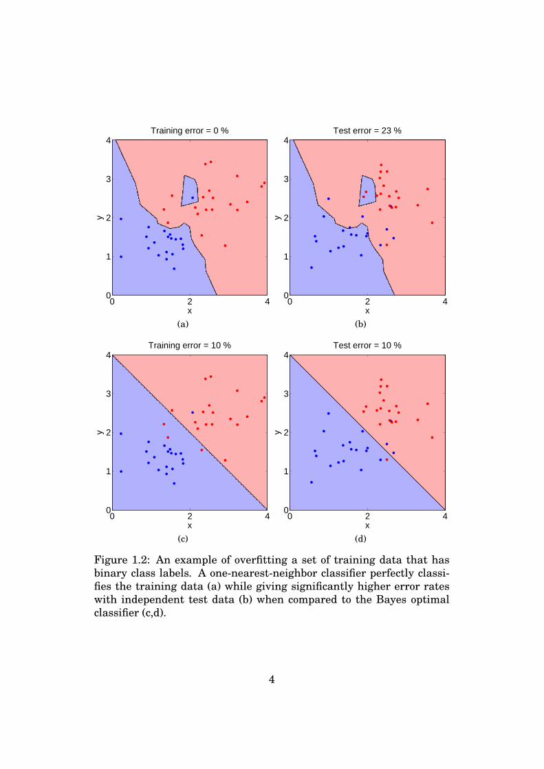
Figure 1.2: An example of overfitting a set of training data that hasbinary class labels. A one-nearest-neighbor classifier perfectly classi-fies the training data (a) while giving significantly higher error rateswith independent test data (b) when compared to the Bayes optimalclassifier (c,d).

4

Overfitting has been demonstrated in Figure 1.2 by using a toy ex-ample. Blue and red dots represent some 2-d training data that hasbeen randomly generated from two Gaussian distributions with dif-ferent means. The background color shows the corresponding decisionareas as learned by a one-nearest-neighbor classifier (Figure 1.2a) or asgiven by an optimal Bayes classifier knowing the underlying data dis-tributions (Figure 1.2c). The nearest neighbor classifier always resultsin a perfect training performance. However, bad generalizability canbe expected, as noticed when comparing against the optimal classifier.Indeed, by drawing new samples independent of the training samples,the misclassification error of the nearest neighbor classifier gets sig-nificantly higher compared to the optimal classifier (Figures 1.2b and1.2d).

1.2 Introduction to Linear ClassificationOne of the simplest classification models is the linear model, whichassigns a binary class label c ∈ {1, 2} to the classified sample accordingto a score value given by the linear combination of the set of d featuresx ∈ Rd and a bias term such that

c =

{1, if β0 + βTx < 02, otherwise , (1.1)

where θ =(β0,β

T)T are the model parameters [2, Chap. 5]. The lin-

ear model is easily extended to the multiclass case as shown later inSection 2.2.

Linear models are convenient because they are easy to interpret andtheir behaviour is widely studied. Linear models have planar decisionboundaries like the line shown in the 2-d binary classification case inFigure 1.2c. In multiclass cases, the decision boundaries are piecewiseplanar honeycomb-like structures.

Popular linear classification methods include linear discriminantanalysis (LDA) [6], support vector machines (SVM) [7] with linear ker-nels, and, the topic of this thesis, logistic regression. While all thesemethods share the same linear classification model in Equation 1.1,they are different in how the model parameters θ are learned from thetraining data. In addition, there can be a difference in how the con-tinuous score value β0 + βTx is interpreted. In LDA, for example, themodel parameters are learned by assuming the data to be normally

5

distributed and then maximizing the class separation, while, in SVM,decision boundaries are formed by maximizing the margin between theclasses. In logistic regression, the parameters are estimated such thatthe posterior probability of the model given the training data is max-imized. When comparing logistic regression and LDA, logistic regres-sion makes fewer assumptions about the features and is consideredmore robust. The topic has been considered, e.g., by Press and Wil-son [8] in the 70’s. There is also a section about choosing between lo-gistic regression and LDA in Hastie’s book [9, Sec. 4.4.5].

−5 0 50

0.5

1

t

P(t)

Figure 1.3: The logistic function.

As the first step towards understanding the basics of the logisticregression classifier, let’s start by reviewing the logistic function

P (t) =1

1 + exp(−t)(1.2)

and its graph in Figure 1.3. The idea of the logistic regression model isto use the logistic function to map the linear combination of the set ofd features x ∈ Rd into an estimate of the probability that x belongs tothe cth class. Thus, logistic regression is a form of probabilistic classifi-cation. This has been illustrated by the diagram in Figure 1.4.

The logistic regression model is a special case of a feedforward neu-ral network [10] with a single neuron. The lack of hidden neuron layersin the network makes logistic regression a linear classifier unlike neu-ral networks in general. If seen as an extension of linear regressionwith a logistic link function, logistic regression belongs to the family ofgeneralized linear models (GLM) [11]. The logistic function allows the

6

x1

x2

xd

1

2

d

0

p(c|x)P( )

Figure 1.4: The two-class logistic regression model is a generalized lin-ear model with a logistic link function P . It is also equivalent with afeedforward neural network with a single neuron.

modeling of binomially distributed response variables instead of Gaus-sians like in ordinary linear regression. Other link functions in placeof the logistic function can be used for modeling different response dis-tributions, e.g., exponential or Poisson distributions.

From the viewpoint of probabilistic classification, logistic regressionis a form of probabilistic discriminative modeling [12], where the modeldirectly estimates the probability p(c|x)1 of a certain class c given thedata x. In an alternative method of generative modeling [12], bothclass-conditional probability distributions p(x|c) and the priors p(c) aremodeled separately. After this, Bayes’ theorem is applied in order tofind the posterior class probabilities for making the decision:

p(c|x) ∝ p(c)p(x|c). (1.3)

A typical example of a generative model is the naïve Bayes classifier,which assumes the features to be conditionally independent given theclass labels. In this case, the Bayes’ rule can be written as

p(c|x) ∝ p(c)d∏

i=1

p(xi|c). (1.4)

The benefit compared to Equation 1.3 is that the class conditional prob-ability distributions are now one-dimensional and can easily be mod-eled, e.g., by fitting Gaussian distributions. Common ways to model the

1In this thesis, notation p(c|x) is used interchangeably, depending on the context,with notation P (C = c |X = x) for denoting the conditional probability of the realiza-tion c of the random variable C given that the random variable X has value x.

7

prior distribution p(c) is to assume uniform class probabilities or to usethe training data to estimate the ratio between different class labels.

It is a widely discussed topic whether discriminative or generativemodels should be preferred in general [13, 14, 15, 16, 17, 12]. Gener-ative models are versatile and can be used, e.g., for sampling of new(x, c) pairs [12]. Also, because generative models model the completejoint distribution, handling partially missing data is more intuitivecompared to discriminative models. In a typical classification problem,however, discriminative models are generally considered more prac-tical over the generative models. Typically, there are fewer parame-ters to estimate and model errors become less significant [4, Sec. 4.3].In most practical applications of supervised learning such as those inChapter 4, features like sampling are not needed and only the clas-sification performance matters. In these applications, discriminativemodels such as logistic regression are justified and likely to give betterresults compared to generative models.

1.3 ObjectivesThe objective of this thesis is to show the versatility and practicalityas well as study the limitations of a simple linear logistic regressionmodel combined with sparsity promoting coefficient regularization thatworks as an automated feature selector embedded in the parameterestimation procedure. This is done in an application oriented mannerin real machine learning applications.

In this thesis, the simplicity of the linear model is emphasized overmore complex classifiers. The usefulness of the interpretability of thelinear model coefficients is stressed in several application cases. Fur-ther, a simple model structure helps to avoid overfitting, which is anextremely important aspect to be taken into account when well per-forming and generalizable classifiers are desired, which is usually thecase. Another important objective of this thesis is to discuss overfittingavoidance by means of proper model validation and automatic param-eter selection in Section 3.2.

Specific claims in this thesis include:

• A comprehensively engineered initial feature set combined withautomatic feature selection and a linear classification model out-performs other methods in several selected application fields in-volving supervised classification.

8

• Logistic regression with sparsity promoting coefficient estimationcan be used for combining feature selection and classifier train-ing. The benefit is that the feature set gets optimized for the spe-cific model resulting in improved performance compared to otherstate-of-the-art methods in several selected application fields.

• Combining feature selection and coefficient estimation also re-duces the computational load because no explicit feature selec-tion algorithms are required. This improvement can be crucial inapplications requiring short response times.

• Due to the simplicity of the model, the model coefficients are eas-ily interpretable bringing extra knowledge, which is useful in sev-eral selected application cases.

• Iteratively improving a classification model by means of subse-quent cross-validation may lead to overly optimistic results andshould be avoided when possible.

Support for the above claims are given by means of the results obtainedin the application cases of Section 4. Majority of these results are basedon those presented in peer-reviewed publications listed in Section 1.5.The last item in the above list is related to parameter selection but canalso be consider in a more general context as discussed in Section 3.2.

1.4 OutlineThe rest of this thesis is organized as follows: First, in Chapter 2, thelogistic regression model and the basics of sparse coefficient estima-tion are reviewed. Next, Chapter 3 focuses on how to measure theperformance of a pre-trained classification model (Section 3.1) and howto do model validation, parameter selection, and to avoid overfitting(Section 3.2). The most of the scientific results of this thesis are pre-sented in Chapter 4 that introduces and gives the results on applyingthe sparse logistic regression classifier in several different applicationfields. Finally, in Chapter 5, some concluding remarks are given.

9

1.5 Publications and Author’sContribution

Most of the results in this thesis are based on the author’s first-authorpublications [18, 19] and the co-authored publications [20, 21, 22, 23].No other dissertation is based on these publications. Author’s contri-bution to each of the publications is the following.

In [18], the author is the responsible author for the design, imple-mentation, and validation of the prediction model as well as runningthe experiments. Prof. Matti Nykter gave insights into the applicationfield and provided text for the introductory part. Assoc. Prof. HeikkiHuttunen provided parts of the text, especially in the discussion part,and participated in the design of the experiments. Dr. Tech. PekkaRuusuvuori contributed in the preprocessing of the data, conducted thegating experiments, and provided parts of the text in the material sec-tion. The results related to [18] are presented in Section 4.3.

The author is the main contributor of the design, implementation,experimentation, and writing of [19], which provides the backgroundand the baseline method for object detection in inkjet printed electron-ics manufacturing covered in Section 4.2. The other contributors areVille Pekkanen who was responsible for operating the printer in thepractical experiments, Kalle Rutanen and Pekka Ruusuvuori who par-ticipated in the design of the algorithms, Risto Rönkkä who partici-pated in the design of the experiements and provided text for the intro-ductory part, and Heikki Huttunen who participated both in the designof algorithms and experiments, especially by providing the general ideaof the connection pad detection pipeline.

A new approach for object detection involving logistic regressionsegmentation is given in [20], where the author has contributed in thedesign, implementation, and data collection of the experiments as wellas in providing text for the logistic regression classification part. In ad-dition to the printed electronics case, the image segmentation frame-work introduced in [20] is utilized in the cell segmentation case in Sec-tion 4.1.2.

In [21] and [22], the author has provided parts of the text and al-gorithm implementation, and contributed into the model validationand design of experiments. Majority of the scientific input has beenprovided by Heikki Huttunen, while Jukka-Pekka Kauppi and JussiTohka have mainly contributed into the issues and text concerning theapplication field. In [22], the author has designed and implemented

10

the experiments for illustration of the wrong and right ways to applycross-validation as also discussed in Section 3.2.4. The actual applica-tion case of [22] is given in Section 4.4.

Finally, in [23], the author was responsible for producing part of theresult figures for the experiments. In addition, he participated in thedesign of experiments. The topic of using Bayesian error estimationin selection of the logistic regression model and the related results arediscussed in Section 3.2.3.

11

Chapter 2

Logistic RegressionClassification and SparseParameter Estimation

In the following sections, first, a brief introduction into some historicalaspects of logistic regression classification is given in Section 2.1. Next,a definition of the logistic regression model is given for both binary andmulticlass cases in Section 2.2. Finally, in Section 2.3, methods for pa-rameter estimation, i.e., ways for training the model by using trainingdata, are given. The theory of logistic regression classification is moreextensively presented, e.g., in the book by Hastie et al. [9, Sec. 4.4].

2.1 BackgroundLogistic regression is a well established classification method taughtto students on a basic university statistics course. The logistic func-tion given in Equation 1.2 in Section 1.2 dates back to the 19th centurywhen a Belgian mathematician Pierre François Verhulst first used itfor modeling the growth of human population after realizing that theconventional exponential model would eventually lead into impossiblylarge values [24].

Since its first introduction, the logistic function has been used inseveral applications related to exponential growth limited, e.g., by theamount of available resources. Pioneering studies using the logisticfunction include modeling of the population growth, modeling productconcentrations in autocatalytic chemical reactions, and modeling death

12

rate as a function of drug dosage. It has since been used for varioustasks in economics, epidemiology, and social sciences, for instance. [24]

The employment of the logistic function in applications of logisticregression classification emerged during the advent of the computerera in the 70’s. Similar to that with the logistic function, pioneeringapplications came from fields such as medical, economics, and socialsciences. Daniel McFadden earned the Nobel Prize in Economical Sci-ences in 2000 from his work in developing the theory of discrete choicemodeling. A great deal of the theory in choice modeling owes to themultinomial logistic regression model. [24]

More recent advances in logistic regression classification are relatedto coefficient regularization [25, 26, 27, 28]. Via regularization, one canhandle issues often present in practical machine learning problemssuch as small sample size, high sample dimensionality, and redun-dancy between features. Especially sparsity promoting regularizationhas proven useful in practical machine learning applications, whichmakes it an interesting tool in the context of this thesis. With ”sparse”we mean some of the parameter estimates being equal to zero. Thisresults in a logistic regression model, where only a subset of the initialfeatures are chosen into the model. Such an elegantly combined fea-ture selection and classification frees us from using traditional explicitfeature selection methods that are often time consuming and do notnecessarily result in good predictive power.

2.2 Logistic Regression ModelLike mentioned in Section 1.2, logistic regression uses the logistic func-tion in Equation 1.2 to model the probability of the occurrence of anevent. In a binary classification problem, the probability of class onegiven the d-dimensional feature vector x ∈ Rd is modeled as

p(C = 1 |X = x) =1

1 + exp(−(β0 + βTx

)) =exp

(β0 + βTx

)1 + exp

(β0 + βTx

) , (2.1)

where β0 ∈ R and β ∈ Rd are the model parameters, collectively de-noted by the parameter vector θ =

(β0,β

T)T .

The generalization of the logistic regression model into multinomialcase for classes c = 1, . . . , K is achieved by modeling the probability of

13

each class separately as

p(c |x) =exp

(βc0 + βT

c x)

1 +∑K−1

k=1 exp(βk0 + βT

k x) , c = 1, . . . , K − 1,

p(K |x) =1

1 +∑K−1

k=1 exp(βk0 + βT

k x) , (2.2)

where p(c |x) is a short hand notation for p(C = c |X = x)1. There arenow (K−1)(d+1) model parameters, which we denote in a single vectoras θ =

(β10,β

T1 , . . . , β(K−1)0,β

TK−1

)T . Notice that the denominator in themodel is chosen such that the probabilities p(c |x), c = 1, . . . , K, sum upto one.

Equation 2.2 gives the traditional way of defining the multinomiallogistic regression model. An alternative and slightly more convenientdefinition is given by the symmetric model that models the class prob-abilities as

p(c |x) =exp

(βc0 + βT

c x)∑K

k=1 exp(βk0 + βT

k x) , c = 1, . . . , K. (2.3)

The parameter vector is now of the form θ =(β10,β

T1 , . . . , βK0,β

TK

)T ,i.e., there are d + 1 parameters more than in the traditional model.This makes the symmetric model ambiguous. Indeed, adding a con-stant value to the bias terms βk0 does not change the model. It turnsout, however, that the redundancy will not be a problem when usingconstrained optimization, i.e., regularization, in estimating the modelparameters. Thus, the symmetric model is used in the experiments ofthis thesis unless otherwise stated.

Regardless of whether the traditional or symmetric model is used,the predicted class c = 1, . . . , K for sample x is given by the maximumof the class probabilities, i.e.,

c = argmaxc

p(c |x). (2.4)

The above maximization problem is equivalently written as

c = argmaxc

log (p(c |x)) = argmaxc

gc(x), (2.5)

i.e., as a maximization problem of the discriminant functions gc(x),which, in the case of the traditional model, are defined as

gc(x) =

{βc0 + βT

c x , c 6= K0 , c = K

(2.6)

1We use similar notation where useful in the future

14

and in the case of the symmetric model as

gc(x) = βc0 + βTc x. (2.7)

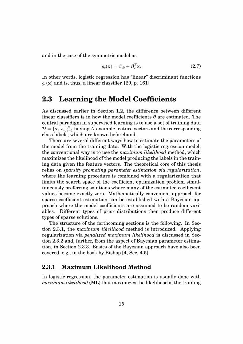
In other words, logistic regression has ”linear” discriminant functionsgc(x) and is, thus, a linear classifier. [29, p. 161]

2.3 Learning the Model CoefficientsAs discussed earlier in Section 1.2, the difference between differentlinear classifiers is in how the model coefficients θ are estimated. Thecentral paradigm in supervised learning is to use a set of training dataD = {xi, ci}Ni=1 having N example feature vectors and the correspondingclass labels, which are known beforehand.

There are several different ways how to estimate the parameters ofthe model from the training data. With the logistic regression model,the conventional way is to use the maximum likelihood method, whichmaximizes the likelihood of the model producing the labels in the train-ing data given the feature vectors. The theoretical core of this thesisrelies on sparsity promoting parameter estimation via regularization,where the learning procedure is combined with a regularization thatlimits the search space of the coefficient optimization problem simul-taneously preferring solutions where many of the estimated coefficientvalues become exactly zero. Mathematically convenient approach forsparse coefficient estimation can be established with a Bayesian ap-proach where the model coefficients are assumed to be random vari-ables. Different types of prior distributions then produce differenttypes of sparse solutions.

The structure of the forthcoming sections is the following. In Sec-tion 2.3.1, the maximum likelihood method is introduced. Applyingregularization via penalized maximum likelihood is discussed in Sec-tion 2.3.2 and, further, from the aspect of Bayesian parameter estima-tion, in Section 2.3.3. Basics of the Bayesian approach have also beencovered, e.g., in the book by Bishop [4, Sec. 4.5].

2.3.1 Maximum Likelihood MethodIn logistic regression, the parameter estimation is usually done withmaximum likelihood (ML) that maximizes the likelihood of the training

15

data D = {xi, ci}Ni=1, i.e., by maximizing the likelihood function

L(θ;D) =N∏i=1

p(ci|xi). (2.8)

Equivalently, one can maximize the log-likelihood function

l(θ) = logL(θ;D) =N∑i=1

log p(ci|xi). (2.9)

The log-likelihood function in Equation 2.9 behaves nicely from op-timization point of view because it is concave and has analytical firstand second derivatives. Thus, a standard Newton-Raphson method canbe used for iteratively finding θ that maximizes l(θ). In the Newton-Raphson method, a new θ(k+1) is found by updating the previous solu-tion θ(k) as

θ(k+1) = θ(k) +H−1(θ(k))∇l(θ(k)). (2.10)

Above, ∇l = (∂l/∂θ1, ∂l/∂θ2, . . .)T is the gradient function and H is the

Hessian, i.e., a matrix with elements Hij = ∂2l/∂θi∂θj.Inverting the Hessian matrix H in Equation 2.10 can be compu-

tationally expensive. Quasi-Newton methods can be used for directlyapproximating the inverse of the Hessian in an iterative manner. Oneof the most used and efficient quasi-Newton algorithms uses the BFGS(Broyden-Fletcher-Goldfarb-Shanno) update or its limited memory ver-sion L-BFGS. [30]

Another approach is to approximate the Hessian matrix by its ex-pectation. This allows the reformulation of the maximum likelihoodproblem into a weighted least squares problem, where the weights de-pend on θ (see details from [31]). This type of problem is then effi-ciently solved by using the iteratively reweighted least squares (IRLS)algorithm [32], which in each iteration solves a weighted least squaresproblem and then updates the weights for the next iteration accord-ingly. A downside in IRLS is that it requires plenty of training data inorder for the approximation of the Hessian to be accurate. As a rule ofthumb, the training data should contain at least ten times more sam-ples per class compared to the number features [33].

2.3.2 RegularizationIn many real life classification problems, we have an arbitrary set ofinitial features. Some of the features can be highly redundant and

16

some may not include any relevant information from the viewpoint ofthe classification task. In such a case, the ML problem may becomeill-posed. Another problem occurs when the training data is linearlyseparable. In this case, the log-likelihood in Equation 2.9 saturatesand any separating hyperplane will do for the ML [4, p. 206]. Thisinevitably decreases the classifier’s ability to generalize.

A traditional solution for the feature redundancy problem is to in-troduce a feature selection or dimension reduction step that tries toonly take account the relevant features or make the features uncorre-lated or independent. However, a more sophisticated way to go is to usesparsity promoting parameter regularization. This kind of regulariza-tion works as an embedded feature selector simultaneously handlingthe saturation problem in the case of linearly separable data.

For simplicity, let’s consider the binary classification problem wherethe parameter vector of the logistic regression classifier is of the formθ = (β0,β

T )T . The simplest sparsity promoting regularization tech-nique defines a maximum value t ≥ 0 allowed for ||β||1 =

∑dk=1 |βk|, i.e.,

the `1 norm of the coefficient vector β:

maxθ{l(θ;D)} , s.t. ||β||1 ≤ t. (2.11)

Equivalently, this can be formulated in the Lagrangian form as a pe-nalized maximum likelihood (PML) problem [9, sec. 3.4.2]:

maxθ{l(θ)− λ||β||1} , (2.12)

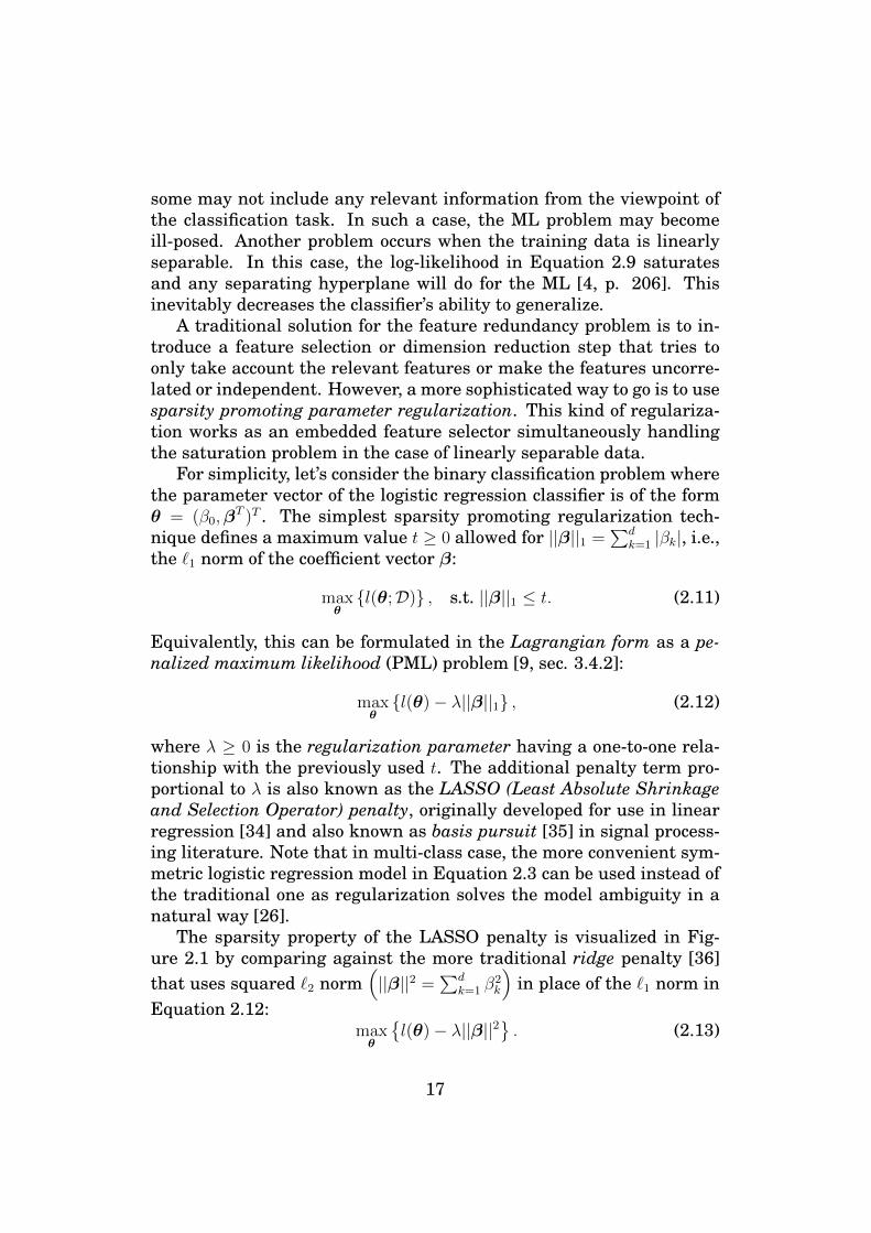
where λ ≥ 0 is the regularization parameter having a one-to-one rela-tionship with the previously used t. The additional penalty term pro-portional to λ is also known as the LASSO (Least Absolute Shrinkageand Selection Operator) penalty, originally developed for use in linearregression [34] and also known as basis pursuit [35] in signal process-ing literature. Note that in multi-class case, the more convenient sym-metric logistic regression model in Equation 2.3 can be used instead ofthe traditional one as regularization solves the model ambiguity in anatural way [26].

The sparsity property of the LASSO penalty is visualized in Fig-ure 2.1 by comparing against the more traditional ridge penalty [36]that uses squared `2 norm

(||β||2 =

∑dk=1 β

2k

)in place of the `1 norm in

Equation 2.12:max

θ

{l(θ)− λ||β||2

}. (2.13)

17

1

2

-1 0 1 2 3-1

0

1

2

3

ML

L1

L2

Figure 2.1: The contour lines show an example of the log-likelihoodfunction to be maximized. Regularization sets constraints to the searchspace. In `2 regularization the searched area is circular, in `1 regular-ization it is diamond shaped.

The contour lines in the image show an example of the log-likelihoodfunction with respect to model parameters β1 and β2 in a 2-d case. TheML solution βML has been marked with the black plus sign. Regu-larization sets constraints into the parameter space, which are shownas a circular area in the case of `2 regularization and as a diamondshaped area in the case of `1 regularization. The constrained maxi-mization problem is to find the optimum inside these areas. The dia-mond shaped area of the `1 penalty favors solutions that reside on oneor more of the coordinate axes. This makes some of the coefficient val-ues equal to zero. Increasing the value of the regularization parameterλ makes the diamond smaller and increases the number of zero coef-ficients. In many real life problems, the feature selection property ofthe LASSO penalty results in better classifier generalizability over theridge penalty, especially when irrelevant features are present [37].

18

Sometimes it is desirable to adjust between the `2 regularizationthat averages the features by jointly bringing the model coefficientstowards zero and the `1 regularization that has the feature selectionproperty. An efficient and practical way for achieving this is to useelastic net regularization [28], which optimizes the log-likelihood as

maxθ

{l(θ)− λ

(α||β||1 + (1− α)||β||22

)}. (2.14)

The penalization term is now a convex combination of the `1 norm andthe squared `2 norm of the coefficient vector β. The mixing parameterα ∈ (0, 1) is used for determining the proportions between the differenttypes of regularizations. Setting α = 1 produces the LASSO penalty(Equation 2.12) and setting α = 0 produces the ridge penalty (Equa-tion 2.13).

Similar to that in the unregularized case, the IRLS algorithm canbe used for solving the regularized problems as well. However, sim-ple and resource friendly cyclical coordinate descent methods such asglmnet [26] and the sparse multinomial logistic regression (SMLR) al-gorithm [38] have been proven to work fast and practically, especiallyin large scale problems like text [39] and microarray data classifica-tion [40]. Especially the glmnet algorithm proposed by Friedman etal. [26] is versatile and fast. It can be used in the case of linear regres-sion, binary logistic regression, as well as multiclass logistic regressionand works together with `1, `2, and elastic net penalties. The algorithmestimates the model coefficients efficiently for complete regularizationpaths with different λ values, which are needed for automatic selectionof λ, e.g., by using cross-validation or BEE (see Section 3.2 and [23]).The computational efficiency of the glmnet algorithm is shown to out-perform competing methods. Its time complexity in one cycle of up-dating each coefficient estimate is O(dN) compared to O(d3 + dN) ofthe IRLS algorithm and the SMLR algorithm if using `1 penalty. Un-less otherwise stated, glmnet is used for coefficient estimation in theapplications of this thesis.

2.3.3 Bayesian MethodsIn the previous section, parameters θ of the logistic regression modelwere considered to be fixed but unknown. In Bayesian framework,however, the parameters are considered random variables with someprior distribution. In the case of logistic regression, complete Bayesianinference is intractable [4, Sec. 4.5]. However, it is possible to find

19

the maximum a posteriori (MAP) point estimate for θ and apply, e.g.,Markov Chain Monte Carlo (MCMC) sampling if a variance estimate isneeded [41].

According to the Bayes rule, the posterior probability p(θ|D) is pro-portional to the product of the likelihood and the prior, i.e.,

p(θ|D) =p(D|θ)p(θ)

p(D)∝ p(D|θ)p(θ), (2.15)

where p(D|θ) = L(θ;D) is the likelihood of the data (as given in Equa-tion 2.8), p(θ) is the prior distribution of the coefficients θ, and p(D) isthe prior distribution of the training data D.

The MAP estimator is achieved by maximizing p(θ|D). Notice, thatp(D) is independent of θ, which makes the MAP equivalent to maxi-mizing p(D|θ)p(θ). Further, by taking a logarithm, one can see that theMAP estimator is equivalent of the PML estimator where the penaliza-tion term equals to the negative of the logarithm of the prior p(θ):

arg maxθ{p(D|θ)p(θ)} = arg max

θ{l(θ) + log p(θ)} . (2.16)

In the following, the key idea is to assume different shapes for the priordistribution p(θ) in order to attain different types of regularization.

First, consider the case where the coefficients βk (k = 1, . . . , d) areassumed independent and normally distributed with zero mean andequal variance σ2, i.e.,

p(βk) =1√

2πσ2exp

(− β2

k

2σ2

)(2.17)

⇒ p(θ) =d∏

k=1

p(βk) =1

(2πσ2)d/2exp

(−||β||

2

2σ2

). (2.18)

In many real life problems all the coefficients βk rarely have equal priorvariance because the corresponding features can have rather differentscales. In practice, however, this is taken care of by standardizing thefeatures to have zero mean and unit variance.

Now, assuming that σ2 is known, the logarithm of the prior in Equa-tion 2.18 can be written as

log p(θ) = −||β||2

2σ2− d

2log 2πσ2. (2.19)

Thus, the MAP estimator becomes equal to

arg maxθ{l(θ) + log p(θ)} = arg max

θ

{l(θ)− ||β||

2

2σ2

}, (2.20)

20

i.e., equivalent to the PML estimator with ridge penalty and the regu-larization parameter equal to λ = 1/(2σ2). In other words, the more weallow the coefficients βk to vary around zero the less we apply regular-ization.

Further assume that the variance σ2 is not fixed but for each vari-able it is independently distributed according to the exponential distri-bution, i.e.,

p(σ2) =

{r exp (−rσ2) , σ2 > 00 σ2 ≤ 0

, (2.21)

where r > 0 is the rate parameter. Integrating out σ2 reveals thatthe prior p(θ) is now a multivariate Laplace distribution or a doubleexponential

p(βk) =

∫ ∞−∞

p(βk|σ2)p(σ2) dσ2 =λ

2exp(−λ|βk|) (Laplace t.f.2) (2.22)

⇒ p(θ) =d∏

k=1

p(βk) =

(λ

2

)d

exp(−λ||β||1), (2.23)

where λ =√

2r is now the rate parameter [43, 39, 27]. With this priorthe corresponding MAP estimator becomes equivalent to the PML esti-mator with LASSO penalty having the regularization parameter equalto λ. Thus, the Laplace distribution works as a sparsity promotingprior equivalent to the `1 penalty in PML estimation.

As the next step, let’s further assume that, instead of being fixed,also λ is a random variable. Interesting results are obtained if we as-sume λ to be the same for each βk and to have a non-informative Jef-freys prior p(λ) ∝ 1/λ [25]. By marginalizing Equation 2.23 over λ, theprior probability p(θ) becomes

p(θ) =

∫ ∞−∞

p(θ|λ)p(λ) dλ =1

2d

∫ ∞0

λd−1 exp(−λ||β||1) dλ

=1

2d||β||d1

∫ ∞0

td−1 exp(−t) dt =Γ(d)

2d||β||d1, (2.24)

where Γ(x) =∫∞0tx−1 exp(−t) dt is the gamma function [25]. In the

above integration, a change of variables (λ = t/||β||1, dλ = dt/||β||1) isperformed in order to pull out the gamma integral.

2The integral in Equation 2.22 can be carried out by noticing that, when choos-ing s = β2

k/2, prior p(βk) is equal to the Laplace transformation F (s) of functionf(t) = − r√

2πt−

32 exp

(− rt). See [42] for details.

21

As a result, there are no unknown regularization parameters in theposterior probability p(θ|D) and the MAP estimator becomes

arg maxθ{l(θ) + log p(θ)} = arg max

θ{l(θ)− d log ||β||1} , (2.25)

i.e., equivalent to the PML problem with penalty term d log ||β||1.From a practical point of view, using the prior in Equation 2.24 re-

sults in a computationally fast way for doing sparse coefficient esti-mation. This is because there is no need for a time consuming cross-validation step normally used for selecting the regularization parame-ters. In addition, a possible source of selection bias by parameter tun-ing can be avoided [44]. Cawley and Talbot [25] have shown that, ina large scale gene selection problem, replacing the MAP estimator’sLaplace prior with the one in Equation 2.24 reduces their computa-tion time from two days to two minutes while the model generalizationperformance is almost the same in both cases.

βk ~ N(0,σ2)

σ2 fixed

λ fixed

σ2 ~ Exponential(λ2/2)

λ ~ Jeffreys

Prior

p(θ)Gaussian Laplace Γ(d)/(2||β||1)

d

Penalty

term ||β||2/(2σ2) λ||β||1 d log||β||1

Figure 2.2: The diagram shows a hierarchy leading to three differentshapes for the prior probability p(θ) attained by different choice of thepriors of its hyper parameters.

22

As a conclusion for the above introduced Bayesian priors p(θ) andthe penalty terms in the corresponding PML problems, see Figure 2.2.Further prior models have been proposed by Caron and Doucet [45]who introduced a general form gamma prior for σ2 that was shownto give sparse estimates and reproduce both Laplace (Equation 2.23)and Jeffreys (Equation 2.24) priors as special cases. They also showedthat, in linear regression, the general gamma prior gave better resultsthan the other sparsity promoting priors. However, two hyper param-eters needs to be chosen by cross-validation, which makes the methodless practical compared to Laplacian prior (one parameter) and Jeffreysprior (no parameters).

2.4 Markov Random Field PriorsIn many applications involving classification, the sample points oftenshare some sort of dependencies, e.g., spatially or temporally. Exploit-ing these dependencies is tempting and can potentially result in signif-icant improvements in the classification performance.

Graphical models [4, Chap. 8] offer a probabilistic tool for model-ing dependencies between random variables and are commonly usedin machine learning to model spatial and temporal relationships be-tween the classified samples. Graphical models are characterized by agraph representation where the random variables correspond to nodesthat are connected by vertices indicating direct conditional dependen-cies between the variables. An example of a graphical model is thehidden Markov model (HMM), which is often used in speech process-ing for linking together the subsequent phonemes or words such thattheir prior distribution follows that of in the spoken language [46].

HMM is an example of a typical type of a graphical model, namely,a Bayesian network. In Bayesian networks, the dependencies are di-rected and acyclic and, as such, are suitable for modeling temporal de-pendencies where future events cannot affect the past. In image anal-ysis, neighboring pixel intensities have spatial dependencies that canwork in any direction. A corresponding way to exploit the class priorknowledge in 2-d is to apply another type of a graphical models, namelyMarkov random fields (MRF). In MRF the dependencies are undirectedand can be cyclic. [4, Chap. 8]

The application that we are interested in this thesis is image seg-mentation, i.e., classifying each individual image pixel into either fore-ground or background. The key idea in using the MRF prior is to as-

23

sume that the prior class distribution of each pixel follows the Markovprinciple, i.e., it depends on the classes of the neighboring pixels butonly on the nearest ones.

c1 c2 ...

V(1,2)(c1,c2)

s t

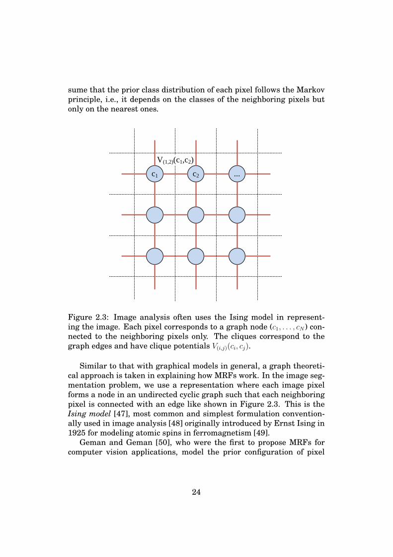
Figure 2.3: Image analysis often uses the Ising model in represent-ing the image. Each pixel corresponds to a graph node (c1, . . . , cN ) con-nected to the neighboring pixels only. The cliques correspond to thegraph edges and have clique potentials V(i,j)(ci, cj).

Similar to that with graphical models in general, a graph theoreti-cal approach is taken in explaining how MRFs work. In the image seg-mentation problem, we use a representation where each image pixelforms a node in an undirected cyclic graph such that each neighboringpixel is connected with an edge like shown in Figure 2.3. This is theIsing model [47], most common and simplest formulation convention-ally used in image analysis [48] originally introduced by Ernst Ising in1925 for modeling atomic spins in ferromagnetism [49].

Geman and Geman [50], who were the first to propose MRFs forcomputer vision applications, model the prior configuration of pixel

24

classes c = (c1, . . . , cN)T by using the Gibbs distribution

p(c) ∝ exp

(−∑i

Vi(c)

), (2.26)

where i goes through the set of cliques3 of the graph and Vi(c) are socalled clique potentials.

When using the Ising model, the cliques simply correspond to theedges connecting each pixel. In this thesis, a definition of clique poten-tial equivalent to that used by Borges et al. [51] is used. This resultsin a simplified form p(c) defined as

p(c) ∝ exp

γ∑(i,j)

δ(ci − cj)

, (2.27)

where (i, j) go through the cliques (each pair of neighboring pixels) and

δ(x) =

{1, x = 00, x 6= 0

(2.28)

is the unit impulse function. In the Equation 2.27, equal labels ci and cjfor neighboring pixels clearly increase the value of the prior, thus, cre-ating a smoothing effect by favoring segmentations with a large num-ber of neighboring pixels having the same class label. The amount ofsmoothing is controlled by using the constant γ > 0.

Combining the MRF prior in Equation 2.27 with a pixelwise logisticregression classifier has been proposed by Borges et al. [51] and, fur-ther, by Ruusuvuori et al. [20]. The problem is that we would like tofind the pixel labeling c that maximizes the posterior probability withthe MRF prior, i.e.,

c = arg maxcp(x|c)p(c), (2.29)

where p(x|c) is the likelihood of the data with labels c and p(c) as de-fined in Equation 2.27. However, instead of the likelihood p(xi|ci), logis-tic regression estimates posterior probabilities p(ci|xi) for each pixel i.This is resolved by using Bayes formula in the unusual direction [51]:

p(xi|ci) = p(ci|xi)p(xi)/p(ci), (2.30)3A clique is a subset of the graph nodes where all nodes are directly connected

with each other.

25

or, if further assuming conditional independence and discarding theconstant term p(xi):

p(x|c) ∝∏i

p(ci|xi)

p(ci). (2.31)

If we further assume equal class probabilities, the denominator canalso be omitted. This way we will end up with the definition of themaximum a posteriori (MAP) segmentation:

c = arg maxc

p(x|c)p(c)

= arg maxc

∑i

log p(ci|xi) + γ∑(i,j)

δ(ci − cj)

. (2.32)

c1 c2 ...

V(1,2)(c1,c2)

s t

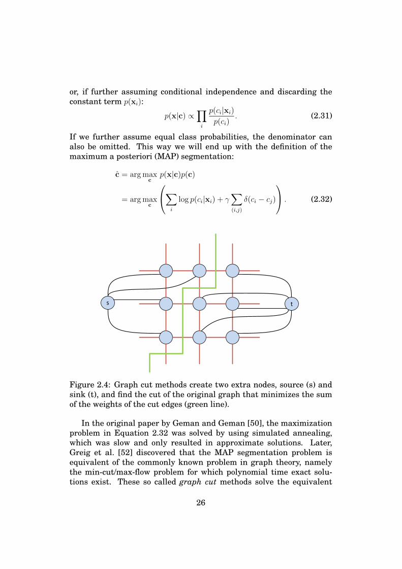
Figure 2.4: Graph cut methods create two extra nodes, source (s) andsink (t), and find the cut of the original graph that minimizes the sumof the weights of the cut edges (green line).

In the original paper by Geman and Geman [50], the maximizationproblem in Equation 2.32 was solved by using simulated annealing,which was slow and only resulted in approximate solutions. Later,Greig et al. [52] discovered that the MAP segmentation problem isequivalent of the commonly known problem in graph theory, namelythe min-cut/max-flow problem for which polynomial time exact solu-tions exist. These so called graph cut methods solve the equivalent

26

problem of splitting a graph into two disconnected parts such that theforeground and background nodes are in different partitions as illus-trated by Figure 2.4. Generally, graph cut algorithms applied for im-age segmentation using the Ising model have time complexity ofO(N3),which can be potentially high. However, a fast implementation forgraph cuts that can operate near to real-time speed in normal computervision applications has been proposed by Boykov and Kolmogorov [53].This algorithm is also used in this thesis.

In this thesis, MRFs are used in a supervised image segmentationsetting as a spatial prior in a pixelwise logistic regression classifiercombined with automated feature selection by means of `1 regulariza-tion [20]. Graph cuts are used for fast computation of the image seg-mentation. This type of segmentation framework will be introducedlater in Section 4.1 together with experiments in spot detection fromcell images (Section 4.1.2) and object detection in inkjet printed elec-tronics manufacturing (Section 4.2).

27

Chapter 3

Model Selection and ErrorEstimation

There are two basic cases where it is important to have an idea aboutthe performance of a classification model. First, we would like to knowabout the classifier’s ability to generalize on data not seen during thetraining phase. Second, we often want to compare the model with othermodels in order to improve it or to be able to choose the best one amongdifferent models. Comparing classifiers is a bit easier task compared tomeasuring the absolute generalization performance because only therelative performance needs to be known.

This chapter introduces methods for estimating the model error andselecting the best performing model among many models. First, in Sec-tion 3.1, error or performance measures used for measuring the good-ness of trained classifiers are defined. Second, in Section 3.2, meansfor comparing and validating different models with each other are pre-sented.

3.1 Measuring Model PerformanceThere exists a vast number of different metrics for measuring the per-formance of a classification model. Both in measuring absolute gener-alizability and relative performance, it is important to pay attention tothe choice of the used error or performance measure such that it cor-responds to what one really wants to measure. In addition, many per-formance measures only work with binary class labels and cannot beused in a multiclass setting. Thus, the choice of the used performance

28

measure depends mainly on the application and user needs. Next, aset of performance and error metrics are introduced.

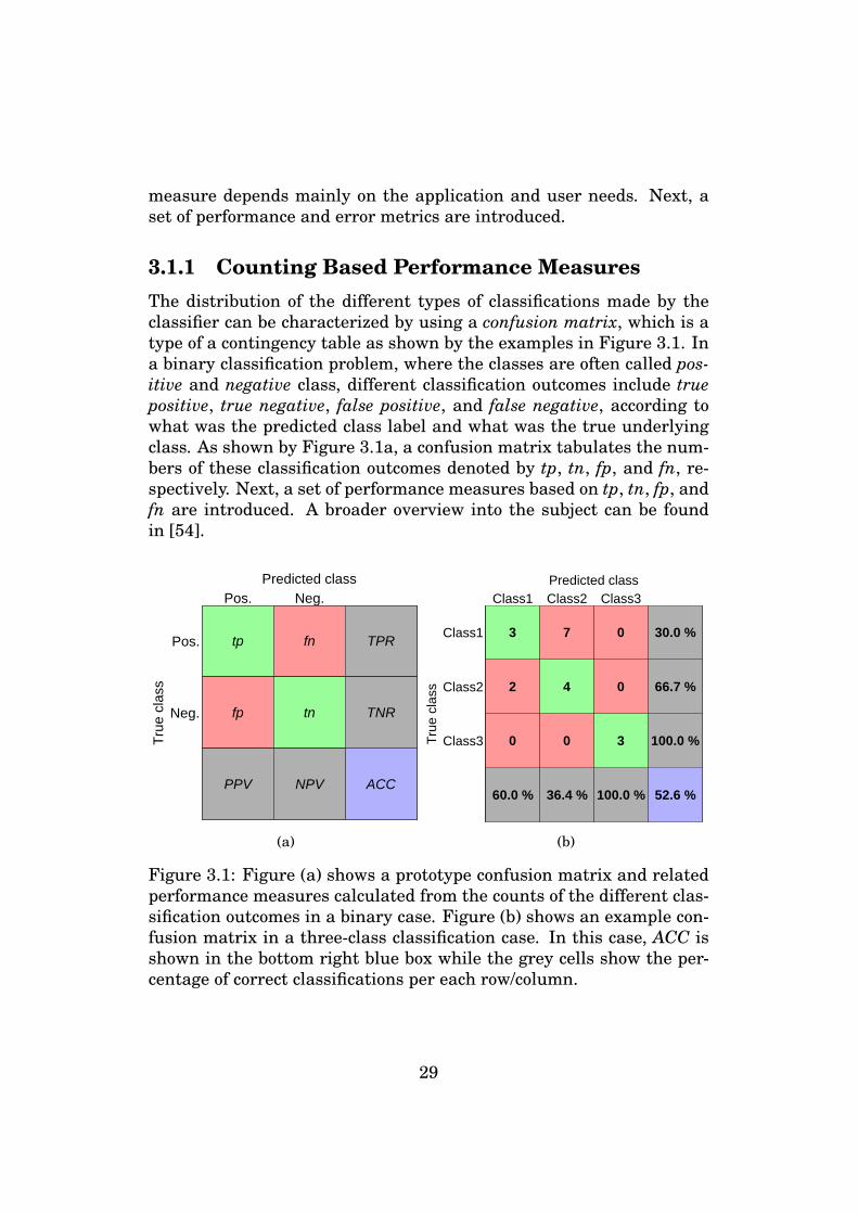
3.1.1 Counting Based Performance MeasuresThe distribution of the different types of classifications made by theclassifier can be characterized by using a confusion matrix, which is atype of a contingency table as shown by the examples in Figure 3.1. Ina binary classification problem, where the classes are often called pos-itive and negative class, different classification outcomes include truepositive, true negative, false positive, and false negative, according towhat was the predicted class label and what was the true underlyingclass. As shown by Figure 3.1a, a confusion matrix tabulates the num-bers of these classification outcomes denoted by tp, tn, fp, and fn, re-spectively. Next, a set of performance measures based on tp, tn, fp, andfn are introduced. A broader overview into the subject can be foundin [54].

Pos. Neg.

Pos.

Neg.

tp fn

fp tn

ACC

TPR

TNR

PPV NPV

Predicted class

True

clas

s

(a)

Class1 Class2 Class3

Class1

Class2

Class3

3 7 0

2 4 0

0 0 3

52.6 %

30.0 %

66.7 %

100.0 %

60.0 % 36.4 % 100.0 %

Predicted class

True

clas

s

(b)

Figure 3.1: Figure (a) shows a prototype confusion matrix and relatedperformance measures calculated from the counts of the different clas-sification outcomes in a binary case. Figure (b) shows an example con-fusion matrix in a three-class classification case. In this case, ACC isshown in the bottom right blue box while the grey cells show the per-centage of correct classifications per each row/column.

29

We start by introducing the simplest and often the most relevantperformance measure in a classification task: the percentage of cor-rectly made classifications. We call this the classification performance(or accuracy (ACC)) and define it simply as the ratio of correct classifi-cations from all classifications:

ACC =tp + tn

tp + tn + fp + fn. (3.1)

The classification performance is often shown in the bottom right cellof the confusion matrix as seen in Figure 3.1.

While classification performance measures the overall accuracy ofthe classifier, it loses information about the distribution of true/falsepositives/negatives. Different performance measures have been devel-oped for measuring different types of errors. Four basic measures arederived from the ratio of correct classifications from each row or col-umn of the confusion matrix. These measures are the true positive rate(TPR) (or recall or sensitivity)

TPR =tp

tp + fn, (3.2)

true negative rate (TNR) (or specificity)

TNR =tn

tn + fp, (3.3)

positive predictive value (PPV) (or precision)

PPV =tp

tp + fp, (3.4)

and negative predictive value (NPV)

NPV =tn

tn + fn. (3.5)

The naming of the above measures varies according to context. For in-stance, TPR and TNR are often used together to see the distribution ofcorrectly made positive and negative classifications in which case theyare usually referred as sensitivity and specificity. Similarly, when us-ing together PPV and TPR, names precision and recall are often used.

A popular performance measure called the F-score can be derivedby calculating the harmonic mean of precision and recall:

F = 2PPV · TPRPPV + TPR

=2tp

2tp + fn + fp. (3.6)

30

F-score measures the effectiveness of the classifier in making true pos-itive classifications. It is also possible to use a weighted version of theF-score where the proportions of the contribution of precision and recallcan be selected by a choice of weight parameter value. This makes itpossible to tune the F-score according to application needs. Notice thatF-score doesn’t depend on the number of true negatives. This shouldbe noted when using F-score in classification applications.

As shown by the example in Figure 3.1b, the confusion matrix iseasily extended into multiclass case. Also the performance measuresintroduced above can be extended into multiclass by defining tpc, tnc,fpc, and fnc for each class c = 1, . . . , K separately in a one-vs-all man-ner. In other words, tpc is the number of correct classifications intoclass c, tnc is the number of correct classifications into other than classc, fpc is the number of false classifications into class c, and fnc is thenumber of false classifications into other than class c. Using these def-initions, there are two possibilities to calculate the above performancemeasures [55, 54, 56, 57]:

1. Macro-averaging. Calculate the performance measure for eachclass separately and then average.

2. Micro-averaging. Accumulate tpc, tnc, fpc, and fnc over eachclass and calculate the performance measure by using the accu-mulated values.

The difference in the above two approaches is that macro-averagingdiscards the effect of the class sizes while micro-averaging takes alsoaccount the number of instance in each class by weighting the perfor-mance measure in question in a corresponding way.

3.1.2 Order Based Performance MeasuresMany classification methods have a parameter that is used for settinga balance between the sensitivity of positive and negative classifica-tions. Increasing the value of this parameter increases the numberof positive classifications while decreasing it increases the number ofnegative classifications. With a classifier with continuous output suchas the logistic regression classifier, this balance can be controlled bythresholding the classifier output such that values above the thresholdare classified as positives and those under the threshold as negatives.With the logistic regression classifier the threshold should be set to0.5 because the model is designed to produce class probabilities and

31

not some arbitrary score values, for example. However, changing thethreshold is useful when calculating further performance measures asexplained next.

0 0.5 10

0.5

1

FPR (= 1 - specificity)

TPR

(=se

nsiti

vity

)

(a)

0 0.5 10

0.5

1

PPV (= precision)

TPR

(=re

call)

(b)

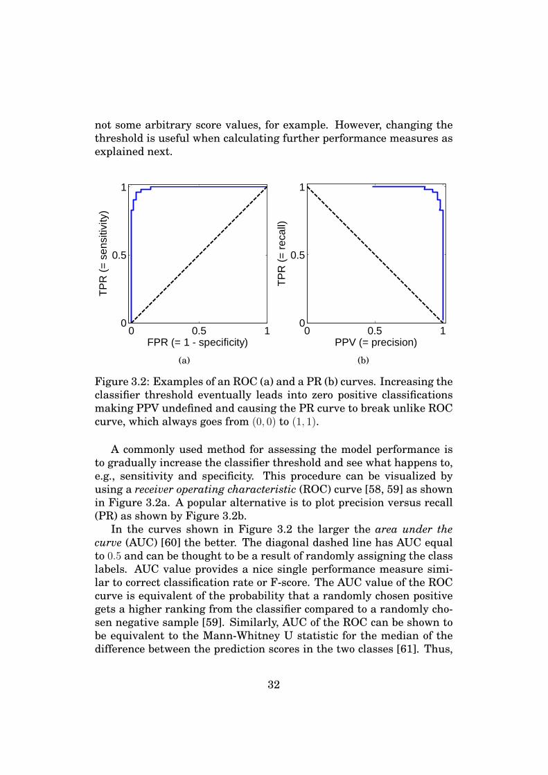
Figure 3.2: Examples of an ROC (a) and a PR (b) curves. Increasing theclassifier threshold eventually leads into zero positive classificationsmaking PPV undefined and causing the PR curve to break unlike ROCcurve, which always goes from (0, 0) to (1, 1).

A commonly used method for assessing the model performance isto gradually increase the classifier threshold and see what happens to,e.g., sensitivity and specificity. This procedure can be visualized byusing a receiver operating characteristic (ROC) curve [58, 59] as shownin Figure 3.2a. A popular alternative is to plot precision versus recall(PR) as shown by Figure 3.2b.

In the curves shown in Figure 3.2 the larger the area under thecurve (AUC) [60] the better. The diagonal dashed line has AUC equalto 0.5 and can be thought to be a result of randomly assigning the classlabels. AUC value provides a nice single performance measure simi-lar to correct classification rate or F-score. The AUC value of the ROCcurve is equivalent of the probability that a randomly chosen positivegets a higher ranking from the classifier compared to a randomly cho-sen negative sample [59]. Similarly, AUC of the ROC can be shown tobe equivalent to the Mann-Whitney U statistic for the median of thedifference between the prediction scores in the two classes [61]. Thus,

32

AUC values give information about the ranking capability of the clas-sifier without considering what the classifier threshold should be andwhat is the absolute classification performance.

Similar to that with the performance measures based on the confu-sion matrix, also AUC can be extended into the multiclass case by ei-ther macro- or micro-averaging. Further, methods for computing mul-tidimensional ROCs and the volume under the surface (VUS) [62, 63]exist. These are out of the scope of this thesis, however.

3.2 Model Validation and AutomaticParameter Selection

The performance measures introduced in the previous section requirethe evaluation of a pre-trained classifier by using a set of test data.The simplest method for error estimation is resubstitution, where thesame data is used both for training and testing [64]. However, sucha procedure often gives overly optimistic results that depend on theclassification model. Generally speaking, the resubstitution error es-timator becomes more optimistic as the classification model gets morecomplex and the number of training samples decreases [65].

In order to avoid optimistic error estimation results, the test datashould be independent of the data used for training the classifier. Inmany cases, however, the amount of available data is small, e.g., due toexpensive or time consuming data collection process. In this case, wewould like to use some procedure to reliably assess the model perfor-mance without losing data from training. In addition to determiningthe generalizability of the model, similar methods can be used for auto-matic selection of model parameters by estimating the relative perfor-mance between subsequent models with different parameter values.

Next, some procedures for model validation and automatic param-eter selection are given. First, in Section 3.2.1, the popular cross-validation method is introduced. After this, rather a similar approachof bootstrapping is given in Section 3.2.2. While both cross-validationand bootstrapping are classification algorithm independent ways to doerror estimation, Section 3.2.3 gives methods targeted for the linearmodel only. Finally, in Section 3.2.4 we discus the potential optimismthat might occur due to misuse of cross-validation and, in Section 3.2.5,we tackle the issue of the effect of the sample size in error estimation.

33

3.2.1 Cross-validationThe simplest way to assess model performance after resubstitution is tosplit the available training data set into two parts and use the first onefor training and the second one for assessing the model performance.If the amount of data is low, the performance estimates will end upbeing pessimistic because only part of the data is used for training. Onthe other hand, we need to have large enough test set in order to getreliable results.

Figure 3.3: K-fold CV splits the whole data into K folds and uses onefold at a time for testing and the rest for training.

The next step from simply splitting the data in two parts is to usecross-validation (CV) methods [2, sec. 9.6.2]. In K-fold CV (see Fig-ure 3.3) the data is split into K approximately equal parts, or folds,which are all used as the test set one by one while the remaining K − 1folds are used for training. Thus, training and testing is done K timesafter which the results are combined, e.g., by averaging. A special caseoccurs when K equals to the number of training samples. This is calledthe leave-one-out (LOO) CV because each sample gets tested one by onewhile the other ones are used for training.

The split of the data in CV is usually done randomly. Sometimesstratification is used to make the distribution of class labels approx-imately equal in each fold. This is especially useful in cases wherethere is a low number of samples available per class. Fixing the seedin the random number generator ensures repeatable results but alsorestricts us to a particular split of data, which is not necessarily veryrepresentative of the underlying data distribution. An alternative is toapply Monte Carlo repetitions, i.e., repeat the CV with different splitsto reduce the variance of the results.

CV is a simple and popular way for the assessment of model per-formance. It is also non-parametric in the sense that it doesn’t makeany assumptions about the tested model and, thus, can easily be used

34

for comparing models of different types. The downside in CV is that itcan easily become computationally expensive because of the repeatedtraining and testing steps. There are also other things one needs to becareful at when doing CV. These are discussed in more detail in Sec-tion 3.2.4.

3.2.2 BootstrappingSimilar to CV, bootstrapping [66, 67] divides the data set of N samplesinto training and test sets. In bootstrapping, however, the training datais chosen among all the samples by randomly sampling N samples withreplacement (the bootstrap sample) while the left out samples are usedfor testing. The procedure is repeated by using independent replicatesof the bootstrap sample in order to get a Monte-Carlo estimate of thedesired performance or error measure.

Randomly choosing N samples with replacement among N samplesresults in a training set of size equal to (1− exp(−1))N ≈ 0.632N on theaverage. Compared to N , this is rather small and easily leads to biasederror estimates [64]. This bias can be alleviated by using the 0.632bootstrap estimator [67], which is calculated as the weighted average ofthe resubstitution estimate εresub and the normal bootstrap estimate ε0:

εb632 = (1− 0.632)εresub + 0.632ε0. (3.7)

The problem in the 0.632 bootstrap estimator is that it uses the resub-stitution error, which, like mentioned earlier, is optimistic dependingon the classification model [68].

3.2.3 Parametric MethodsUnlike CV, the parametric methods introduced in this section don’t re-quire splitting of the data. Instead, given the entire training data setand some properties of the classification model, the parametric meth-ods return a single value inferring something about the model perfor-mance and generalizability. Usually, however, some assumptions needto be made, e.g., about the distribution of the data.

AIC

The Akaike information criterion (AIC) [69] is an information theoreti-cal tool to measure the relative information loss due to using a trained

35

classifier model to predict the class labels instead of applying the trueunderlying labeling process. AIC is defined as

AIC = −2l(θ;D) + 2d∗, (3.8)

where l(θ;D) is the log-likelihood for the trained model (the definitionwas given in Section 2.3.1) and d∗ is the number of free parametersof the model (the number of non-zero classifier coefficients). As shownby the above equation, the information loss gets higher as likelihooddecreases or the number of parameters increases. Because AIC onlymeasures the relative information loss, it is suitable for model selec-tion, not for estimating absolute performance or error.

BIC

One of the most used statistical error estimators in addition to AICis the Bayesian information criterion (BIC) [70] developed from theBayesian perspective to estimate the posterior probability of the model.Recently, Chen and Chen [71] have developed the extended BIC (EBIC)that is better suited for high dimensional ill-posed problems. For asparse logistic regression classifier, EBIC is defined as

EBIC = −2l(θ;D) + d∗ log(N) + 2d∗δ log(d), (3.9)

where l(θ;D) is the log-likelihood (see Section 2.3.1), d∗ is the num-ber of free parameters of the model (the number of non-zero classifiercoefficients), N is the number of training samples, and d is the dimen-sionality of the data. Parameter δ ≥ 0 is used for tuning the sensitivityof EBIC for number of selected features. The higher is the value of δthe stronger is the effect of the number of selected features compared tothe data likelihood term. In the experiments, we use δ = 0.5, which hasbeen reported as being a good compromise in many applications [71].

Although derived from different principles, AIC and BIC share sim-ilarities as noticed by looking at their equations (3.8 and 3.9). Thepractical difference is that BIC tends to penalize the number of param-eters more strongly compared to AIC.

BEE

Another Bayesian method for classifier error estimation, namely theBayesian minimum mean-square error estimator (BEE), was recently

36

introduced for a binary classification problem using discrete classi-fiers [72] and linear classifiers such as the logistic regression classi-fier [73]. BEE is a minimum mean-square error (MMSE) estimatorestimating the classification error

BEE = p(C = 1)ε1 + (1− p(C = 1))ε2, (3.10)

where p(C = 1) is the prior probability of class 1 (negative class) and ε1and ε2 are the probabilities of false positive and false negative classifi-cations, respectively.

Assuming that the class conditional data distributions are Gaus-sian and that the class covariance matrices follow the inverse-Wishart-distribution, [73] gives a closed form solution for BEE in the case oflinear classifier with parameters β0 and β (see Section 2.2 for the lin-ear classification model). In this thesis, a simple scaled identity co-variance model is assumed for the class conditional densities and non-informative class prior is used. In our experiments, the covariancesand the means of the class conditional densities are further limited ina minimal way by setting ν = 0, κ = 0, and S = 0. See more detailsin [73]. Now, consider the usual sample estimates for the class means

µc =1

Nc

∑k: ck=c

xk (3.11)

and covariance matrices

Σc =1

Nc − 1

∑k: ck=c

(xk − µc)(xk − µc)T , (3.12)

where Nc is the number of samples in class c = 1, 2. The above assump-tions lead to εc being defined as

εc =1

2

1 + sgn (A)B

A2

A2 + (Nc − 1) tr(

Σc

) ;1

2, α

, (3.13)

wheresgn(z) =

{−1, z < 0

1, z ≥ 0(3.14)

is the sign function,

B(x; a, b) =Γ(a+ b)

Γ(a)Γ(b)

∫ x

0

t(a−1)(1− t)(b−1) dt (3.15)

37

is the regularized incomplete beta function, tr(·) is matrix trace, and αand A are real-valued quantities summarizing the data and the classi-fier such that

α =d(d+ 1)

2− 1 (3.16)

and

A =β0 + βT µc

||β||

√Nc

Nc + 1. (3.17)

The mathematical derivation for Equation 3.13 given the above as-sumptions is found in the Appendix D of [73].

In a recent study, we have shown that BEE is especially efficient inproblems, where the amount of training data is small and CV methodssuffer from splitting the data [23]. This topic, along with experiments,is further discussed in Section 3.2.5. We have made our MATLABimplementation of the above BEE formulation available at https://sites.google.com/site/bayesianerrorestimate/.

3.2.4 Pitfalls in Cross-ValidationHastie et al. [9] describe a wrong and right way to do CV. The key ideais that the different folds in CV need to be independent in order toprevent the results from being optimistic. In scientific literature, toooften all the data is used for making decisions about the model afterwhich CV is run. In particular, Hastie et al. concentrate on featureselection: The incorrect strategy consists of three steps [9, Sec. 7.10.2]:

1. Find a subset of good predictors that exhibit strong correlationwith the class labels.

2. Using only this subset, design a classifier.

3. Use CV to tune the model and estimate the prediction error.

The problem above is that all the data is used in the first step, thus,producing optimistic error estimates and worse performance for trulyindependent test data. However, it turns out that the misuse can be alot more subtle and difficult to recognize as we will see.

Following the example of [9], we did the following experiment [22].

1. Generate N = 100 samples of random data of dimension d = 30.

2. Generate binary class labels for the samples, also at random.

38

3. Honest way: Design a classifier and calculate the classificationerror using 10-fold cross validation. In this example we used a3-nearest-neighbor (3NN) classifier.

4. Cheating (version 1): Violate the CV principles as in [9]:

(a) Find the single feature that gives the smallest classifier errorwith 3NN.

(b) Estimate the error as in step 3, but with the best feature only.

5. Cheating (version 2): Use 10-fold CV twice:

(a) Estimate the classification error for each single feature using10-fold CV.

(b) Estimate the error using 10-fold CV as in step 3, but withonly the best feature found in step 5a.

6. Cheating (version 3): Proceed as in step 5, but change the ran-dom seed between the two CVs, thus, using different division ofsamples.

The above procedure was repeated 1000 times and the histograms ofthe estimated classifier performances (ACC) for each case (honest andcheating 1–3) are shown in Figure 3.4. It can be seen that the honestway without any feature selection estimates the accuracy in a realisticmanner, i.e., the performance estimate is close to random chance 0.5.However, all three ways of cheating give an optimistic estimate of theperformance clearly above 0.5.

One might think that using cross-validation in the feature selectionstep (cheating versions 2 and 3) would be less harmful than using alldata (cheating version 1) because the best performing feature in eachCV fold is selected by testing on an independent set of data. How-ever, it turns out that the double-CV approaches are clearly the mostdangerous ways of incorrectly assessing the classification performance.There are at least two reasons for this to happen: 1) The illusion aboutthe independence of the CV folds is broken right after the first fea-ture selection CV when the CV results of the best performing featuresare combined by averaging. 2) Both the first and the second CV use 10folds, which allows the first feature selection CV to exploit the informa-tion about the exact sample size that is going to be used in the secondCV that estimates the final classification performance.

39

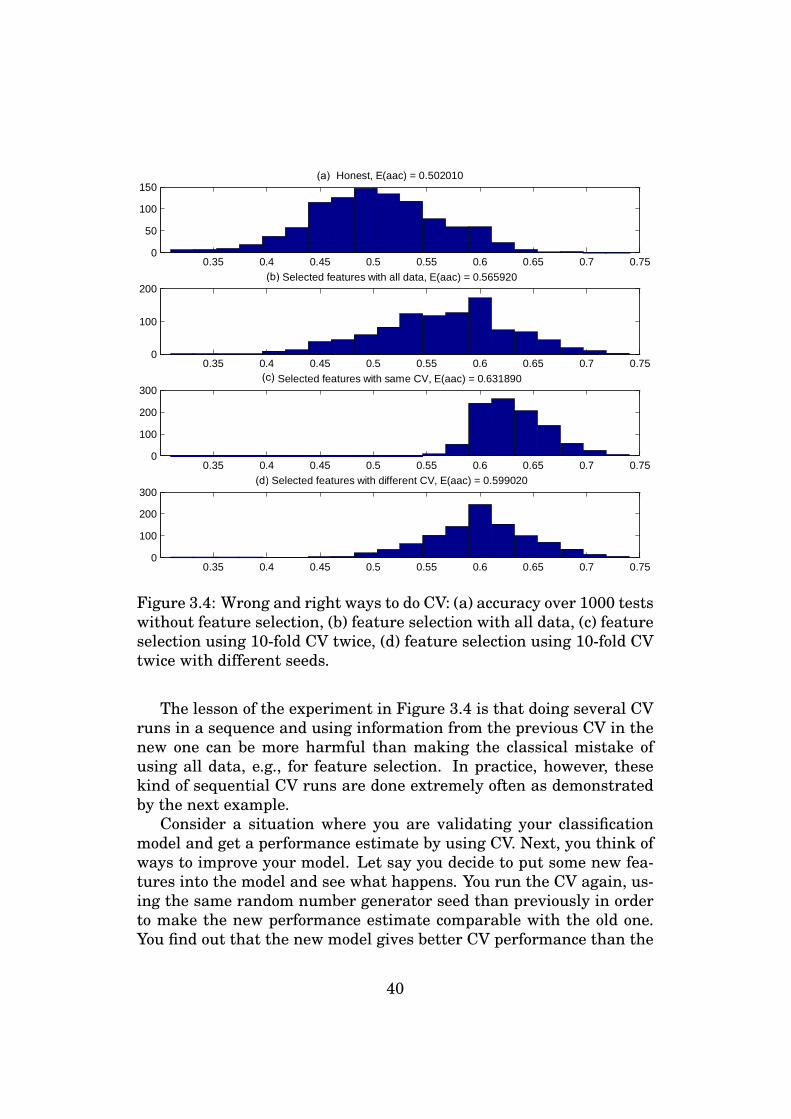
0.35 0.4 0.45 0.5 0.55 0.6 0.65 0.7 0.750

50

100

150Honest, E(aac) = 0.502010

0.35 0.4 0.45 0.5 0.55 0.6 0.65 0.7 0.750

100

200Selected features with all data, E(aac) = 0.565920

0.35 0.4 0.45 0.5 0.55 0.6 0.65 0.7 0.750

100

200

300Selected features with same CV, E(aac) = 0.631890

0.35 0.4 0.45 0.5 0.55 0.6 0.65 0.7 0.750

100

200

300Selected features with different CV, E(aac) = 0.599020

Figure 3.4: Wrong and right ways to do CV: (a) accuracy over 1000 testswithout feature selection, (b) feature selection with all data, (c) featureselection using 10-fold CV twice, (d) feature selection using 10-fold CVtwice with different seeds.

The lesson of the experiment in Figure 3.4 is that doing several CVruns in a sequence and using information from the previous CV in thenew one can be more harmful than making the classical mistake ofusing all data, e.g., for feature selection. In practice, however, thesekind of sequential CV runs are done extremely often as demonstratedby the next example.

Consider a situation where you are validating your classificationmodel and get a performance estimate by using CV. Next, you think ofways to improve your model. Let say you decide to put some new fea-tures into the model and see what happens. You run the CV again, us-ing the same random number generator seed than previously in orderto make the new performance estimate comparable with the old one.You find out that the new model gives better CV performance than the

40

previous one, which will naturally make you choose the new set of fea-tures over the previous one. At this point, however, by comparing thenew CV performance with the old one, you are doing exactly what wasshown to be the most wrong way of doing CV. In an extreme case, youcould even iterate the same procedure until you had found the perfectset of features for your particular CV and division of data into folds.In fact, this is how classical feature selection methods such as floatingselection [74] work; by sequentially adding or removing features andassessing the classification performance at each step by using CV.

The unfortunate thing in the above example is that it is hard, oreven impossible, to prevent this kind of optimism from happening. Howdo you improve your model if you are not allowed to make any decisionsbased on previous CV runs? There is no solution but to try to make de-cisions that are likely to create as little optimism in the results as pos-sible. For instance, tweaking a couple of model parameters and seeinghow the CV estimate changes is clearly less harmful than systemat-ically going through all possible feature combinations and ultimatelychoosing the one that gives the best CV result.

3.2.5 The Effect of Sample Size in Error EstimationAn important factor affecting the choice of the used error estimator isthe sample size, which is what we have studied in a recent article [23].Figure 3.5 shows an example of the effect of the training sample sizeon the performance of different error estimators in a model selectionproblem where the task is to find a suitable value for the regulariza-tion parameter λ in the `1 regularized logistic regression model (seeEquation 2.12). The experiment has been conducted by using a high-resolution ovarian cancer data set from the FDA-NCI Clinical Pro-teomics Program Databank1. The data set is used in a binary classifica-tion task of diagnosing whether the patient has ovarian cancer or not.The data comes from laser desorption and ionization (SELDI) proteinmass spectrometry and has 15000 features corresponding to ion inten-sity levels at different mass/charge values. There are 216 patients inthe data set, 95 controls and 121 ovarian cancers.

Five different estimators for estimating the model classification per-formance have been tested in Figure 3.5: BEE, EBIC, and 2-fold, 5-fold,and 10-fold CVs. The vertical axis shows the difference between theclassification performance of the optimal logistic regression model that

1http://home.ccr.cancer.gov/ncifdaproteomics/ppatterns.asp

41

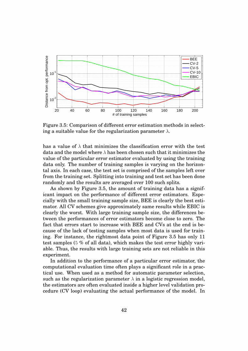
20 40 60 80 100 120 140 160 180 200

10-2

10-1

# of training samples

Dis

tanc

efro

mop

t.pe

rform

ance BEE

CV-2CV-5CV-10EBIC

Figure 3.5: Comparison of different error estimation methods in select-ing a suitable value for the regularization parameter λ.

has a value of λ that minimizes the classification error with the testdata and the model where λ has been chosen such that it minimizes thevalue of the particular error estimator evaluated by using the trainingdata only. The number of training samples is varying on the horizon-tal axis. In each case, the test set is comprised of the samples left overfrom the training set. Splitting into training and test set has been donerandomly and the results are averaged over 100 such splits.

As shown by Figure 3.5, the amount of training data has a signif-icant impact on the performance of different error estimators. Espe-cially with the small training sample size, BEE is clearly the best esti-mator. All CV schemes give approximately same results while EBIC isclearly the worst. With large training sample size, the differences be-tween the performances of error estimators become close to zero. Thefact that errors start to increase with BEE and CVs at the end is be-cause of the lack of testing samples when most data is used for train-ing. For instance, the rightmost data point of Figure 3.5 has only 11test samples (5 % of all data), which makes the test error highly vari-able. Thus, the results with large training sets are not reliable in thisexperiment.

In addition to the performance of a particular error estimator, thecomputational evaluation time often plays a significant role in a prac-tical use. When used as a method for automatic parameter selection,such as the regularization parameter λ in a logistic regression model,the estimators are often evaluated inside a higher level validation pro-cedure (CV loop) evaluating the actual performance of the model. In

42

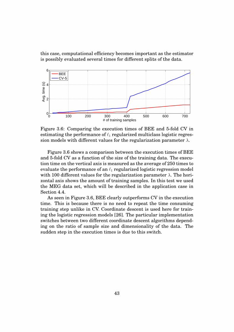
this case, computational efficiency becomes important as the estimatoris possibly evaluated several times for different splits of the data.

0 100 200 300 400 500 600 7000

2

4

6

# of training samples

Avg

.tim

e(s

)

BEECV-5

Figure 3.6: Comparing the execution times of BEE and 5-fold CV inestimating the performance of `1 regularized multiclass logistic regres-sion models with different values for the regularization parameter λ.

Figure 3.6 shows a comparison between the execution times of BEEand 5-fold CV as a function of the size of the training data. The execu-tion time on the vertical axis is measured as the average of 250 times toevaluate the performance of an `1 regularized logistic regression modelwith 100 different values for the regularization parameter λ. The hori-zontal axis shows the amount of training samples. In this test we usedthe MEG data set, which will be described in the application case inSection 4.4.

As seen in Figure 3.6, BEE clearly outperforms CV in the executiontime. This is because there is no need to repeat the time consumingtraining step unlike in CV. Coordinate descent is used here for train-ing the logistic regression models [26]. The particular implementationswitches between two different coordinate descent algorithms depend-ing on the ratio of sample size and dimensionality of the data. Thesudden step in the execution times is due to this switch.

43

Chapter 4

Case Studies

In this chapter, results on real life classification problems where thesparse logistic regression model has been successfully used are intro-duced. The following work is based on publications and data challengesthat the author has been involved in.

Section 4.1 first introduces a general purpose sparse logistic regres-sion based image segmentation framework and a related applicationin the field of cell segmentation from microscope images. Next, inSection 4.2, the same supervised image segmentation approach is ap-plied in object detection in inkjet printed electronics manufacturing.Other applications of sparse logistic regression are related to diagno-sis of acute myeloid leukemia (Section 4.3) and brain signal analysis(Section 4.4). All the introduced application cases use sparse logisticregression, which has proven to be a universal classification methodusable in many application areas.

4.1 Supervised Image SegmentationIn this section, we introduce a general purpose supervised image seg-mentation framework that uses sparse logistic regression for classify-ing each pixel of an image into foreground or background [20] (Sec-tion 4.1.1). Segmentation is used in several applications in the field ofimage analysis. One of these is the segmentation of cells from micro-scope images which is presented in Section 4.1.2.

44

4.1.1 Overview of the Supervised ImageSegmentation Framework

The traditional approach for solving segmentation and detection prob-lems in image analysis is very application oriented. Often the designeris an expert in image analysis techniques. However, the end user ofthe image analysis tool, especially in the field of medical image analy-sis, is usually not too experienced in the field and may lack the skillsfor manual tuning, which is often necessary in order to get satisfactorysegmentation results.

Ground truth

Training images

Generate features

TrainTrained classifier

ImageGenerate features

Classify Graph cutSegmented

image

Trai

nin

g

Test

ing

Figure 4.1: Block diagram of the supervised image segmentationframework.

In [20], we have proposed to use `1 regularized logistic regressiontogether with an MRF spatial prior for a general segmentation task.The approach is supervised, i.e., there are separate training and testphases. These have been illustrated by the block diagram in Figure 4.1.The different stages of processing are explained in the following start-ing from the training stage that has three steps:

• Collecting training data. First, a set of training data needsto be collected for training the classifier. In practical applica-tions this is basically a set of training images together with theirground truth segmentation, e.g., manually created by the user.

• Feature generation. A set of features is generated for eachtraining image pixel by applying a set of manually defined image

45

filters with a range of parameters. The idea is to use a large poolof features from which a good subset is likely to be found for differ-ent types of applications. The features can include, e.g., low passfilters, edge filters, texture features, morphological filters, waveletdecomposition features [75], and local binary patterns [76], all ofwhich are applied with varying parameter values, kernel sizes,etc.

• Training. A binary logistic regression classifier is designed to de-termine if a pixel belongs to the foreground or to the background.The key idea is to use `1 regularization in the coefficient estima-tion in order to automatically select the features that are relevantfrom the viewpoint of the application at hand. The glmnet pack-age [26] is used for coefficient estimation and a proper value forthe regularization parameter λ is chosen by using CV.

The actual classification stage is the following:

• Feature generation. For each image pixel, features are cal-culated. Only the features selected by the regularization in thetraining phase need to be computed. Thus, computationally effi-cient segmentation can be achieved even if the feature set used inthe training phase was large.

• Classification. The trained logistic regression classifier is usedfor predicting the probability of each pixel belonging to the fore-ground.

• Graph cut. The graph cut algorithm is applied to produce theMAP segmentation of the image that combines the MRF spatialprior with the pixel-wise posterior probabilities produced by thelogistic regression model as explained in Section 2.4.

The main idea in the above segmentation framework is that witha comprehensive choice of the initial set of image features, the sametraining and actual segmentation steps can be used in many differentapplications with little effort or special knowledge from the user. Simi-lar ideas for supervised segmentation with feature selection have beenused in pixel classification with hyperspectral images [51, 77] and inbackscatter image segmentation [78]. Of these, the first inputs mul-tichannel images acquired at different wavelengths directly with nofiltering, while the second uses a fixed collection of filters, but selects

46

the most relevant ones with simple forward selection. Moreover, thelatter paper does not estimate the class probabilities, which have asignificant role in our framework. Further, a highly similar approachof discriminative random fields (DRM) has been proposed by Kumarand Hebert [79] who use discriminative logistic regression modelingtogether with a spatial prior. The key difference in this approach isthat the prior probabilities are modeled by using a combination of theIsing model and a data dependent logistic regression model for whichthe coefficients are learned jointly with the pixelwise class probabilitymodel. In our case, however, automatic feature selection is in a cen-tral role. Estimating the coefficients of the pixelwise class probabilitymodel separately from the prior allows us to use conventional learningalgorithms [26] and, thus, efficient `1 regularization for achieving thefeature selection property.

Two real life application cases using the segmentation frameworkare introduced in this thesis: subcellular spot detection (Section 4.1.2)and object detection in inkjet printed electronics manufacturing (Sec-tion 4.2). In addition to these applications, similar approach has beenused in outline-based cell segmentation [80].

4.1.2 Segmentation of Cell ImagesThe first application case utilizing the supervised segmentation frame-work involves detection of subcellular objects from simulated micro-scope images [81]. Reliable automated subcellular object detection isneeded in several applications including interpretation of complex cel-lular phenotypes, analysis of cellular structures from fluorescence andconfocal microscope images, and live-cell tracking [82].

We have applied the proposed supervised segmentation frameworkfor cell segmentation in [20]. In this study, we use simulated cell im-ages instead of real microscope images. The main benefit in using sim-ulated images is in the availability of the ground truth for the numberand locations of the subcellular objects. The simulated image set weuse is designed for benchmarking purposes [82] and publicly availableat http://www.cs.tut.fi/sgn/csb/simcep/benchmark.

The simulated image set contains 20 images with a fixed number ofcells and subcellular objects per cell. An example of a simulated cellimage is shown in Figure 4.2a. The images contain cells with nuclei(blue channel, B), cytoplasmic areas (red channel, R), and subcellularobjects (green channel, G). The segmentation task is to detect the sub-

47

(a) (b) (c)

Figure 4.2: An example of a simulated cell image (a), its gray scaleversion (b), and the estimated probabilities (c) of individual pixels be-longing to a subcellular spot. The probabilities have been attained byapplying a logistic regression model together with a Markov RandomField prior.

cellular objects from a grayscale image obtained by using the standardconversion 0.2989R + 0.5870G+ 0.1140B (Figure 4.2b).

Table 4.1: Features and parameter ranges used in the experiments. Intotal, 106 features were used in this study.

Feature Parameter ValuesGaussian lpf kernel width σ {3, 5, 7, . . . , 83}Unsharp masking kernel width σ {3, 5, 7, . . . , 83}Morphological top-hat kernel size {3, 5, 7, . . . , 83}Morphological bottom-hat kernel size {3, 5, 7, . . . , 83}Masking with h-maxima transform h {3, 5, 7, . . . , 83}Local binary patterns - -Edge enhancement kernel size {3, 5, 7, . . . , 83}Wavelet decomposition depth layer {1, 2, 3}

As an experiment, we estimate the segmentation performance bycomputing the pixel-wise F-score, precision, recall, and the numbersof true positives, false positives, and false negatives between the seg-mentation result and the ground truth segmentation provided by theimage simulator. To avoid optimism in the segmentation performance,the training and testing of the logistic regression classifier is performedin a LOO CV manner such that each of the 20 images in the above im-age set are used for training at a turn and the remaining 19 are used

48

for testing. From each image, 70 foreground and 700 background pixelsare used for training purposes. The initial set of features computed foreach pixel consists of 106 features with different parameters as listedin Table 4.1.

Table 4.2: Subcellular object detection results for simulated images.The results are averaged over the set of test images.

tp fp fn prec. rec. F-score121.11 17.26 20.00 0.876 0.858 0.867

Averaged results over the 20 training and testing iterations areshown in Table 4.2. The table shows the average number of true pos-itives, false positives, and false negatives, and the average precision,recall, and F-score. In [81], a similar analysis was conducted over thesame set of 20 simulated cell images by using 9 conventional segmenta-tion methods. In this study, the majority of the F-scores measuring theoverall segmentation performance were located between 0.4 and 0.6,while the best result was obtained by using Multiscale wavelets [75]that had F-score of 0.63. Clearly, the supervised segmentation frame-work outperforms all these methods with F-score of 0.867.

An example of the output of the logistic regression model (the prob-ability of the foreground) is shown in Figure 4.2c. In this case, thetrained model is extremely easy, namely, regularization only selects 5of the available 106 features into the model. These features are h-maxima masking with h = 63 and h = 68 (H63, H68), edge enhance-ment and top-hat filtering with kernel size 8 (E8, T8), and waveletdecomposition with depth layer 3 (W3). Given the feature vector x =(H63, H68, E8, T8,W3)

T , the model can be written as

p (”foreground” | x) =exp (g(x))

1 + exp (g(x)), (4.1)

where the discriminant function is given as

g(x) = −5.23 + 0.04H63 + 0.003H68 + 0.0007E8 + 0.011T8 + 0.3W3. (4.2)

From the coefficient magnitudes one can see that most of the contribu-tion into the classification rule comes from the wavelet decompositionW3. All the features have been normalized to unit variance in order forthe comparison of the coefficient magnitudes to make sense.

As a conclusion, when it comes to the segmentation of subcellu-lar spots, the proposed supervised segmentation framework seems to

49

clearly outperform the 9 traditional image processing approaches asgiven in [81]. The difference between the performances is further sig-nified by the fact that, in [81], a grid search was conducted in the pa-rameter space of the different segmentation methods in order to tunethem specifically for the 20 tested images, while CV was used in ourexperiments in training the logistic regression model. In addition toimproved segmentation performance, the sparsity property of the reg-ularized logistic regression classifier is able to point out only a handfulof simple image processing operations that are adequate in conductingthe segmentation.

4.2 Object Detection in Inkjet PrintedElectronics Manufacturing

The next application case comes from the field of electronics, namely,inkjet printed electronics manufacturing. In this application, the imagesegmentation framework described in Section 4.1.1 is used as a part ofa computer vision and image processing pipeline. The aim is in auto-matic detection of electronics components from camera images in orderto do online error compensation for the manufacturing process.

The next sections are organized such that, first, in Section 4.2.1, abrief introduction is given to a specific manufacturing method of inkjetprinted electronics and a particular problem that arises due to mis-aligned components. Second, in Section 4.2.2, the concept of computervision controlled printing for fixing this problem is introduced as pro-posed in our earlier work [19]. Finally, methods and results for connec-tion pad detection are given in Section 4.2.3.

4.2.1 Inkjet Printed Electronics and the Problem ofMisaligned Components

Printed electronics is a manufacturing process of electronics where tra-ditional printing devices are used for interconnecting or manufacturingof electronic components. The area of research is relatively new. Unlikeconventionally used etching processes which are based on material re-moval, printed electronics is an additive manufacturing process wherematerial is only added where needed. Advances in new materials allownovel devices, such as flexible displays or Radio Frequency Identifica-tion (RFID) labels to be generated using this approach.

50

One of the fundamental printing technologies is inkjet printing thatrelies on the principles of traditional inkjets with fluid materials tar-geted for electronics. An example application of this technology usesconductive nano particle and dielectric inks to create interconnectionsbetween integrated circuits (ICs) and discrete components that havebeen molded onto the background surface [83]. An example module ofthis kind is shown in Figure 4.3.

(a) (b)

Figure 4.3: A module with four integrated circuits (ICs) (a) ready forprinting of the interconnection layer (b).

One of the most significant challenges in the printed module conceptshown in Figure 4.3 is the accuracy of the manufacturing process. Inac-curacies in the component placement process, molding process relatedmovement, and molding material shrinkage and bending all create er-rors in component locations. The latter category is typically the mostsignificant one, and also the most unpredictable [84].

The errors in the component locations create a misalignment prob-lem between the printed layer and the target surface. Traditional in-spection approaches [85] for printed circuit board (PCB) manufacturingare unsuitable solutions for the problem because, in PCB manufactur-ing, the background materials are rigid, which allows only translationand rotation. In this case, the substrate may shrink or expand caus-ing the components to move with respect to each other. In addition tothe complexity of the transformation, most existing approaches concen-trate on quality control instead of actually fixing the problem.

51

4.2.2 Computer Vision Controlled PrintingIn our earlier work [19], we have proposed a computer vision systemto compensate the errors created due to misaligned components. Com-puter vision enables a fast, easy, and efficient way for analyzing print-outs and printed surfaces. Without the necessity for a physical contact,measuring from an image is especially suited for applications of inkjetprinted electronics. Figure 4.4a shows an example of integrating a com-puter vision system into the printing device in order to detect the exactposition and orientation of an electronics component (Figure 4.4b) onthe printing stage.

Camera Print head

Printed modules

Printer table

Led ring

Frosted glass

Printhead rail

(a) (b)

Figure 4.4: Figure (a) illustrates a camera solution integrated intoa printing device. A mobile printing stage enables a fixed cameramounting. In Figure (b), the orientation of the background componenthas been detected by using computer vision before printing the wiringlayer. Thus, it has been possible to align and modify the print patternto perfectly fit the underlying component.

A software level framework diagram for the computer vision con-trolled correction system is shown in Figure 4.5. Briefly, the idea isthat any distinguishable features in the camera image serve as controlpoints, which are first automatically detected from the image and thenassociated with the corresponding control points in the design. The re-sulting displacement information is then used to modify the printingdata before printing. There are three main stages in the processing:

• Object detection. The processing starts with an image process-ing step where candidate control points are detected from the

52

CorrectionObject Detection

Point Pattern Matching

Displacement data

Detected control points

Camera image

Design control points

Design printing data

Corrected printing data

Figure 4.5: A diagram of a general computer vision based adaptationsystem for inkjet printed electronics that operates on the design print-ing data based on the feedback from the camera image and the imageanalysis pipeline.

camera image. Detected objects usually have relatively simple ap-pearance (e.g., connection pads), which creates plenty of missingand outlier points amongst the candidates. This is the processingblock where supervised learning and classification is applied asdescribed in Section 4.1.1.

• Point pattern matching. After detecting the candidate points,they are associated with their counterparts in the design. The tar-get is to determine the errors in the locations of the control pointsrelative to the design. This is done with a point pattern matching(PPM) algorithm, also known as procrustes analysis [86] in statis-tics. Generally, the PPM problem is rather complex and the state-of-the-art algorithms assume various properties of the point setsto ease the computation. Particularly in the printed electronicscase, however, the control point sets are usually man-made (likethe connection pads on the ICs) and, thus, contain regular andsymmetrical patterns. These kinds of point sets complicate thematching as several well matching subset pairs are present. Wehave proposed a PPM algorithm suitable for these applicationsin [87].

• Correction. The final step is to compensate the detected er-rors. In the example case in Figure 4.3 this means redrawingthe wiring prior to the printing. We have proposed a smooth ge-ometrical transformation that remaps the wiring image withoutaffecting its electrical properties in [88]. In other applications the

53

correction could be done, e.g., by tuning the printer parametersor by merely discarding the module in an inspection style if it’simpossible to apply any correction.

An automated correction system such as the one explained above isessential for improving the manufacturing process of printed electron-ics and making inkjet printing a manufacturing method suitable formass production. The relevant part from the viewpoint of this thesisin such a system is the one utilizing machine learning in the imageprocessing task. This is the topic of the next section.

4.2.3 Detection of Connection Pads from CameraImages

From the viewpoint of this thesis, we are interested in applying ma-chine learning for automatic detection of connection pads on electronicscomponents. This is done in order to solve the component misalignmentproblem of the inkjet printing application as described in the previousSections 4.2.1 and 4.2.2.

A previous method for connection pad detection utilizes a tradi-tional image processing pipeline with the following three steps [19, 89]:

1. IC extraction. The ICs are first located in order to limit the fur-ther processing inside the IC areas only. This is done by usingtemplate matching such that a template image of the correspond-ing module type with known IC locations is matched against thecamera image. A successful match results in the bounding boxesof the ICs. The detected IC boundaries are only approximate sincethe IC misalignment characteristics and the module orientationcan vary between the template and the image under processing.

2. Pad candidate detection. Second, a set of feasible candidatesfor IC connection pad locations is detected. This is done inside thepreviously detected IC areas by, first, highlighting the pad-likeobjects by using template matching and, then, using a modifica-tion of a local thresholding operation called logical level threshold-ing [90]. Logical level thresholding is based on the assumptionthat, after highlighting with template matching, the connectionpads appear as small bright spots. The result of the logical levelthresholding is further filtered by using morphological shape fil-tering and the knowledge of the minimum distance between twoneighboring connection pads.

54

3. Classification. Finally, the set of pad candidates is classifiedinto actual pads and false detections by using supervised classi-fication. Artificial feedforward neural networks are used here af-ter resizing each color image patch of a connection pad candidateinto the size of 6 × 6 pixels. The adjustment of the classificationthreshold affecting the true positive and true negative rates of theclassifier is done by using the knowledge of how many connectionpads should be detected from each IC.

With the above method, high connection pad detection rates canbe achieved [19]. However, the main problem is that the algorithmhas several processing steps that make it computationally inefficientand, thus, unsuitable for online use. In addition, a training step isneeded not only for the neural network classifier but also for templatematching in both IC and pad candidate detection stages. This makesthe practical use of the algorithm rather cumbersome.

As the new connection pad segmentation method, the supervisedsegmentation framework introduced in Section 4.1.1 is proposed. Theidea is to apply logistic regression segmentation for full size cameraimages, take the detected object centroids as detected connection padcandidates, and then use PPM to find individual ICs and exact con-nection pad locations among these. The main benefits compared to thepreviously described method are that

• IC extraction and a separate classification step can be omittedbecause the segmentation framework is efficient enough to workon full size images and the segmentation is reliable enough forthe PPM algorithm to detect individual ICs among the connectionpads detected from the entire image.

• The template matching step used in the previous method for ICextraction cannot handle excess changes in module orientation.Due to the PPM algorithm, the new method is completely rota-tion, translation, and scale invariant (provided that the connec-tion pad formations on the ICs are not rotation symmetric).

• No parameters need to be tuned unlike in the previous method,where each processing step had several parameters such as as-sumed pad size, thresholds and neighborhood size for logical levelthresholding, and shape parameters for morphological filtering.

• Training is easy and can be done with a single module image.Only the ground truth segmentation is needed for training unlike

55

in the previous method, where example templates of the moduleand the connection pads were needed in addition to a comprehen-sive training set of positive and negative connection pad imagesfor training the neural network classifier.

• There’s a significant reduction in algorithm complexity and, thus,in execution time. This enables the use of the proposed algorithmin an online process.

The main benefit of the new approach is in its simplicity and com-putational effectiveness. However, because the entire camera image isconsidered at once and a separate classification step is omitted, it re-sults in more false positives compared to the old method. Fortunately,our experiments have shown that this decrease in detection perfor-mance is tolerable by the PPM algorithm, which couples the individualICs with the connection pad candidate points detected from the im-age. The important point is that the number of missed connection padsshould be as low as possible as this can have a serious effect on theperformance of the PPM algorithm.

(a) (b)

Figure 4.6: An electronics module with 4 ICs used in training a clas-sifier for IC connection pad segmentation. The positive and negativetraining pixels are shown with blue and red dots, respectively. A close-up of a corner of one of the ICs shows connection pads located on thesides of the IC.

An example of the training data and the connection pads to be de-tected is shown in Figure 4.6. In Figure 4.6a, a set of positive (blue)

56

and negative (red) training pixels have been randomly chosen from asingle module image by using the ground truth segmentation, whichhas been obtained by knowing the connection pad radius and locations.In this case the pad locations were obtained by using the old connectionpad detection method and by verifying the result visually. This type oftraining procedure is used in the next experiment where we comparethe segmentation framework with some other choices for connectionpad segmentation.

4.2.4 ExperimentsThe experiments in the cell segmentation case in Section 4.1.2 indi-cated that supervised segmentation can easily outperform many tra-ditional unsupervised algorithms. In this section, the performance ofdifferent supervised methods comparable to the proposed segmenta-tion framework is studied in the segmentation of the connection pads.In addition to the proposed regularized logistic regression combinedwith the graph cut post processing (LR-MRF), also a regularized lo-gistic regression classifier without graph cut (LR) as well as supportvector machine (SVM) and a 10 nearest neighbors (10-NN) classifiersare tested.

We use 12 Mpix color images taken from modules with four ICs asshown in Figure 4.6a. There are a total of 409 connection pads locatedat the sides of each IC. Training data is collected by randomly picking1000 positive and 2000 negative training samples per image as indi-cated by the blue and red dots, respectively. The actual connectionpads can be seen in a close-up of one of the ICs in Figure 4.6b.

The features used in the classifier are the same as used in the cellsegmentation experiments in Section 4.1.2 (see Table 4.1). In the caseof SVM and 10-NN, an additional sequential forward selection stepis used to reduce the amount of intentionally redundant features. Insequential forward selection, single features are selected into the modelaccording to how well they improve the classification performance asestimated by CV in this case [74]. Features are added into the modelwith this fashion until the CV performance stops improving.

In SVM, we use linear kernel, which makes the model linear as inlogistic regression. In 10-NN, `1 norm is used as the distance metric,i.e., the classifier decision is determined by the majority vote of theten nearest neighbors in the training data in terms of the sum of theabsolute differences between the corresponding feature values. In allthe methods, the features are first normalized to unit variance.

57

The performance of the different classifiers is assessed by using asimple two-fold CV such that the classifiers are trained with a singlemodule image similar to that shown in Figure 4.6a and tested withanother one. As the topic is about assessing the segmentation perfor-mance, similarly to that in the cell segmentation case in Section 4.1.2,we settle for measuring the pixel-wise F-score, precision, recall, andtrue positive, false positive, and false negative rates rather than actualconnection pad detection rates.

Table 4.3: Connection pad detection results. The results are averagedover the 2 CV folds.

Method tp fp fn p r F-scoreLR-MRF 24484 87133 460 0.219 0.982 0.359

LR 24683 131573 261 0.158 0.990 0.272SVM 24498 154422 447 0.137 0.982 0.240

10-NN 24566 156066 378 0.136 0.985 0.239

(a) (b) (c) (d)

Figure 4.7: The segmentation result as given by different classificationmethods. (a) LR-MRF, (b) LR, (c) SVM, (d) 10-NN.

The results are given in Table 4.3. As expected, there are plenty offalse positives in each case, which is due to the high amount of smallbright spots other than connection pads in the images. Logistic regres-sion gives slightly less false positives than SVM and 10-NN resultingin better precision and F-score. Using MRF together with the classprobabilities estimated by the logistic regression remarkably reducesthe number of false positives giving it by far the most accurate result.Figure 4.7 shows the part of the segmentation that corresponds to Fig-ure 4.6b. The next step would be to compute the centroids of eachdetected object and apply PPM between these and the connection pad

58

locations of each individual IC in the design data in order to detect theICs and the exact positions of the connection pads in the image.

As a conclusion, the previous experiment shows that the proposedsegmentation framework works well in the connection pad segmen-tation application. Especially, it is shown that the `1 regularizationcombined with logistic regression classification outperforms SVM and10-NN classifiers coupled with sequential forward selection. Combin-ing the MRF prior with the classifier further improves the segmenta-tion result.

4.3 Automated Diagnosis of Acute MyeloidLeukemia

Next, logistic regression is applied for classification of flow cytometrydata in order to diagnose whether a patient has acute myeloid leukemia(AML) or not. The work is based on DREAM6/FlowCAP2 MolecularClassification of Acute Myeloid Leukaemia Challenge organized as apart of the DREAM6 conference in 2011. A 100 % classification accu-racy was achieved on the test set of 20 AML-positive and 160 healthypatients by using a logistic regression classifier with `1 regulariza-tion [91, 92]. Further, the sparsity promoting property of the regu-larization can be used as a valuable tool in evaluating, which of themarkers used in standard flow cytometry are actually needed in thediagnosis. These aspects have been studied in a recent article wherewe have further improved the original challenge submission and con-ducted comparisons with competing models [18].

The forthcoming sections are organized such that Section 4.3.1 givesand introduction to using flow cytometry for AML diagnosis and de-scribes the data set from the DREAM6 AML challenge. Next, Sec-tion 4.3.2 explains methods for AML diagnosis using logistic regressionand some other supervised learning methods. Finally, in Section 4.3.3,some experiments are run.

4.3.1 Flow Cytometry in AML DiagnosisLeukemias are a common malignancy of blood cells emerging from dif-ferent cell types [93]. AML, which is the focus of this work, emergesduring myeloid differentiation. However, the traditional classificationof leukemias relies predominantly on morphologic and cytochemical

59

features of the tumor cells rather than the developmental origin of themalignancy [94].

Blood cancers such as AML are diagnosed with various techniquesincluding features from morphologic, cytochemic, cytogenetic, and flowcytometry. While morphologic, cytochemic, and cytogenetic analysisinclude standard pathological stainings that lead to low dimensionaldata that can typically be interpreted directly under microscope, anal-ysis of flow cytometric data includes the interpretation of more complexhigh dimensional data distributions. Thus, computer assisted decisionsystems are needed to support diagnosis decision making. [95]

Flow Cytometry

Flow cytometry can be used to analyze a large number of individualcells and, thus, is well suited to detect, e.g., cells that express partic-ular cancer related surface markers from blood samples. In the mea-surement process, cells are labeled with fluorescent dye. Fluorescentlabeled cells are guided through a laser beam and the resulting flu-orescence and scatter parameters, typically forward and side scatter,are detected by photo detector. Forward scatter is informative of thecell size and side scatter corresponds to cell granularity. [95, 96]

Table 4.4: Seven tubes (and one unspecified control tube) with differentfluorescence markers (FL1–FL5) are provided in the DREAM6 AMLprediction challenge data set. (Table from challenge web site1.)

Tube FL1 FL2 FL3 FL4 FL51 IgG1-FITC IgG1-PE CD45-ECD IgG1-PC5 IgG1-PC72 Kappa-FIT Lambda-PE CD45-ECD CD19-PC5 CD20-PC73 CD7-FITC CD4-PE CD45-ECD CD8-PC5 CD2-PC74 CD15-FITC CD13-PE CD45-ECD CD16-PC5 CD56-PC75 CD14-FITC CD11c-PE CD45-ECD CD64-PC5 CD33-PC76 HLA-DR-FITC CD117-PE CD45-ECD CD34-PC5 CD38-PC77 CD5-FITC CD19-PE CD45-ECD CD3-PC5 CD10-PC78 N/A N/A N/A N/A N/A

Data from the DREAM6 AML Challenge

Here, we use the DREAM6 AML prediction challenge data that is avail-able at the challenge website1. The data set consists of flow cytometry

1http://www.the-dream-project.org/challenges/dream6flowcap2-molecular-classification-acute-myeloid-leukaemia-challenge

60

measurements taken from 43 AML-positive and 316 healthy patients.The challenge data has seven aliquots or tubes containing 6764 to49370 blood cells that each give a single measurement, i.e., event, perused marker. A different combination of five different markers is mea-sured from each tube. These marker combinations (FL1–FL5) havebeen listed in Table 4.4. Each marker is only present in one of thetubes except for marker CD45, which is included in all of the tubes. Inaddition to fluorescence intensities, forward and side scatter readingsare provided for each tube. Tube number eight is a control tube withnon-specific-binding antibodies. We don’t use this tube for predictionpurposes.

Both raw and preprocessed flow cytometry data are provided in thechallenge data set. For prediction, we use the preprocessed data, whichis compensated/translated using the method described in [97]. The pre-processed data has the forward scatter in linear scale and the side scat-ter and the fluorescence intensities described in Table 4.4 in logarith-mic scale. In addition to the provided preprocessing, some experimentswere conducted with a regression based preprocessing method [98] di-rectly applied for the raw data. However, no improvement was gainedin the results. Thus, all results presented in this thesis are for thepreprocessed contest data, which is available in the contest web site.

4.3.2 Supervised Learning Methods for AMLDiagnosis and Marker Analysis

Similar to that in other classification applications, the basic idea inclassifying flow cytometry data into AML-positive and healthy patientsis to, first, extract a set of features from the data and, then, apply thetrained classifier. A speciality when using flow cytometry data is thatthere are an arbitrary number of individual cells in each tube. Fur-ther, a different combination of markers is measured from each tube.Thus, each tube needs to have a separate processing step that extractsa set of features, which are then combined as a single feature vectorfor the classifier to use. The processing chain using logistic regressionclassification has been illustrated in Figure 4.8.

Because the individual cells and their number varies from measure-ment to another, the features extracted from each tube cannot be cellspecific features but statistics summarizing the joint distribution of themarker values. However, density estimation with multidimensionaldata is known to be a difficult problem. The situation is further com-

61

Figure 4.8: High level diagram on aggregating the flow cytometry datafrom individual test tubes for classification with a logistic regressionmodel.

plicated by the large amount of data points. Thus, good feature engi-neering plays a particularly essential role in this application.

Sparse Logistic Regression with EDF MSE Features

Previously, we have proposed LDA as a supervised dimension reductionstep for working out the problem of multidimensional density estima-tion [91]. In this approach, the distance between the empirical cumula-tive distribution functions (EDF) of the tested sample and those trainedfrom AML and healthy patients are used as features for a sparse logis-tic regression classifier making the diagnosis. The proposed algorithmhas 4 steps:

1. Feature generation. In a later processing stage, the predictionmodel uses rather simple linear operations and distribution com-parison in one dimension. Thus, we cannot expect the model todiscover very complicated relations between the input features.For this reason, the set of features from the initial 5 fluorescenceintensities and 2 scatter features is artificially expanded. Thisis done by taking all possible inverses (7 pcs) and second powers

62

(7 pcs) of the features as well as multiplications (21 pcs) and di-visions (42 pcs) of any combination of two different features. Thisway, the dimensionality of the data is increased from the initial 7to 84.

2. Dimension reduction. To avoid the problem of multidimen-sional (in this case, 84-dimensional) density estimation, LDA isused to map each sample x ∈ R84 generated in the previous stepinto 1-d:

x =(

Σ1 + Σ0

)−1(µ1 − µ0)x. (4.3)

Above, Σ1 and Σ0 are the sample covariance matrices and µ1 andµ0 are the sample means of both AML-positive and healthy train-ing samples, respectively. LDA is a supervised method that usestraining data for finding the linear mapping that best separatesthe AML-positive and healthy populations in 1-d. Applying theLDA significantly reduces the amount of data and allows us touse traditional 1-d methods for distribution comparison.

3. EDF comparison. The actual features from each flow cytometrytube are calculated as the distance of the sample distribution totrained distributions of AML-positive and healthy populations.As the distance measure, we use the mean squared error (MSE)between the EDFs:

ε(c)t =

1

K

K−1∑k=0

[Ft(x0 + k∆x)− F (c)

t (x0 + k∆x)]2, (4.4)

where t = 1, 2, . . . , 7 denote the seven different tubes. Above, Ft(·)is the EDF of the tested tube data after LDA mapping, and F

(c)t

are the corresponding EDFs of the trained healthy tube (c = 0)and the trained AML-positive tube (c = 1). In Equation 4.4 theerror is only evaluated in K discrete points uniformly chosen be-tween points x0 and x0 + (K − 1)∆x. Our validation tests showthat we can use value as low as K = 128 without degrading theclassification performance. We choose x0 equal to the minimum ofthe training samples and ∆x such that x0 + (K − 1)∆x equals tothe maximum of the training samples.In addition to the EDF MSE, also more established distributioncomparison methods were tested including two-sample Cramér-von Mises test [99], Kolmogorov-Smirnov test [100], and Kullback-Leibler divergence [101]. Further, error measures like correlation

63

and MSE between the probability density functions estimatedwith kernel smoothing density estimation were tested. However,based on validation results, EDF MSE gave the best classificationperformance.

4. Classification. Given the 14-dimensional feature vector ε =(ε

(0)1 , ε

(1)1 , . . . , ε

(0)7 , ε

(1)7 )T corresponding to the EDF error measures

of each tube as defined in Equation 4.4, the final classificationinto AML-positive or healthy patient is done by using `1 regu-larized logistic regression. In this application, the implicit fea-ture selection via regularization automatically detects tubes ir-relevant from the diagnosis point of view and excludes them fromthe model. The glmnet package [26] is used for coefficient esti-mation and a proper value for the regularization parameter λ ischosen by using CV.

When using all the available 359 patients in the DREAM6 challengedata set for training the logistic regression classifier with `1 regulariza-tion, the trained classifier can be written as

p (”AML” | ε) =exp (g(ε))

1 + exp (g(ε)), (4.5)

where the discriminant function is given as

g(ε) = −4.5037 + 1.7980ε(0)4 − 1.0845ε

(1)4 − 0.8694ε

(1)5 + 0.0753ε

(0)6 . (4.6)

The remarkable notion above is that the `1 regularization only se-lects 4 of the available 14 features. Further, only tubes 4, 5, and 6 areincluded in the final model making tubes 1, 2, 3, and 7 non informativefrom the diagnosis point of view.

Based on the absolute values of the logistic regression coefficientsin Equation 4.6, tube number 4 (see corresponding markers from ta-ble 4.4) seems to be the most important one. Also tube 5 has a substan-tial effect on the predictor output but only when comparing againstAML-positive (c = 1) patients. Tube number 6 has a similar effecton the healthy patients. However, relatively small absolute coefficientvalue makes tube 6’s contribution rather insignificant. Notice thatcomparing absolute coefficient values makes sense because the simi-larity scores ε(c)i are normalized.

The full regularization path of the above case is shown in Figure 4.9.The final model indicated by the black dashed line is chosen by mini-mizing 10-fold CV error. The EDF distance features from tube 4 are the

64

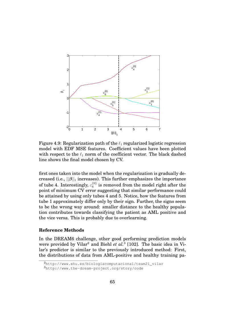
0 1 2 3 4 5 6 7-2

-1

0

1

2

3

|| ||1

i

4{1}

6{0} 1

{1}

1{0}

5{1}

4{0}

Figure 4.9: Regularization path of the `1 regularized logistic regressionmodel with EDF MSE features. Coefficient values have been plottedwith respect to the `1 norm of the coefficient vector. The black dashedline shows the final model chosen by CV.

first ones taken into the model when the regularization is gradually de-creased (i.e., ||β||1 increases). This further emphasizes the importanceof tube 4. Interestingly, ε{0}6 is removed from the model right after thepoint of minimum CV error suggesting that similar performance couldbe attained by using only tubes 4 and 5. Notice, how the features fromtube 1 approximately differ only by their sign. Further, the signs seemto be the wrong way around: smaller distance to the healthy popula-tion contributes towards classifying the patient as AML positive andthe vice versa. This is probably due to overlearning.

Reference Methods

In the DREAM6 challenge, other good performing prediction modelswere provided by Vilar2 and Biehl et al.3 [102]. The basic idea in Vi-lar’s predictor is similar to the previously introduced method: First,the distributions of data from AML-positive and healthy training pa-

2http://www.ehu.es/biologiacomputacional/team21_vilar3http://www.the-dream-project.org/story/code

65

tients are compared against that of the tested patient for each tube.Second, resulting distribution similarity scores are aggregated in a lo-gistic regression model to derive an AML confidence score between 0and 1.

Vilar’s method doesn’t apply explicit dimension reduction for thedata to alleviate the problem of multidimensional density estimation.Instead, the probability density of the 7-dimensional tube data is ap-proximated by using multiple lower dimensional densities. These den-sities are constructed such that only one of the fluorescence markersFL1, FL2, FL4, or FL5 is taken into account in each density estimatewhile fluorescence marker FL3 (which is always CD45 regardless ofthe tube) and forward and side scatters are present in all of the lowdimensional densities. This results in 4 different 4-dimensional dis-tributions instead of one 7-dimensional. In practice, these densitiesare approximated by histograms with 9 bins per dimension uniformlyspaced in logarithmic scale between 100.01 and 100.91 for all but the sidescatter for which the corresponding range is between 102.01 and 102.91.An important feature, found out by our validation tests, is that anysample outside the range of the histogram is considered an outlier anddiscarded.

The comparison of the distributions in Vilar’s method is done byusing Kullback-Leibler divergence [101], i.e., relative entropy. The en-tropies from each tube are combined by simply summing together therelative entropies with the AML-positive population and subtractingthe entropies with healthy population. This total entropy is mappedwith the logistic function to get the final AML confidence score. Interms of logistic regression classification as viewed in this thesis, thismeans that the logistic regression model coefficients are not estimatedfrom training data but fixed such that the relative entropies with AML-positive populations and healthy populations have coefficients equal to1 and −1, respectively. Further, the bias term β0 equals to zero.

Biehl’s method differs from the proposed one and Vilar’s by not try-ing to estimate the full densities of the data. Instead, six statistics;mean, standard deviation, skewness, kurtosis, median, and interquan-tile range, are calculated for each marker and used as features. Forclassification, Biehl uses Generalized Matrix Relevance Learning Vec-tor Quantization. See [102] for details.

66

Sparse Logistic Regression with Simplified Features

In our recent article [18], we have shown that a similar classificationperformance to the introduced logistic regression model with EDF MSEfeatures, and to the methods by Vilar and Biehl et al. can be achievedby simply using mean values of each marker directly as features in thelogistic regression model. That is, the marker intensities in Table 4.4along with the forward and side scatter values are averaged over theevents in each tube creating 49 features. These features are then usedfor training an `1 regularized logistic regression model.

From model analysis point of view, the difference in using markermeans as features compared to the previously proposed EDF MSE fea-tures is that the sparsity promoting regularization now selects individ-ual markers instead of complete tubes when deciding the relevance ofeach feature. In the best case scenario, majority of the normally con-ducted flow cytometry measurements can be completely omitted whenrunning the diagnosis. This is studied in the forthcoming experimentsection along with comparisons of classification performance with otherprediction models.

4.3.3 ExperimentsAs the first experiment, the coefficients of the logistic regression modelwith simple marker mean features are studied. The training is donewith the entire DREAM6 AML challenge data set and `1 regularizationis used in coefficient estimation. The resulting coefficient values corre-sponding to each feature are shown in Figure 4.10. It turns out thatonly 17 of the 49 variables are selected into the model. About half of thecontribution in terms of `1 norm of the coefficient vector comes from thefour most significant markers, which are CD34-PC5 from tube 6, sidescatter from tube 5, and CD16-PC5 and CD13-PE from tube 4. Noticethat comparing absolute coefficient values makes sense because thefeatures have been normalized to zero mean and unit variance.

Figure 4.11 shows the regularization path (a) and the correspondingCV error (b) of the above experiment with respect to the `1 norm of thecoefficient vector β. The vertical dashed lines show the point where thefinal model has been selected. This point has been chosen by findingthe minimum CV error and then using the one-standard-error rule, i.e.,by picking the simplest model whose CV error is at most one standarderror away from the minimum CV error.

67

0 5 10 15 20 25 30 35 40 45 50-1

-0.5

0

0.5

1

IgG1-PE (1)

IgG1-PC7 (1)

Lambda-PE (2)

CD19-PC5 (2) CD8-PC5 (3)

CD15-FITC (4)

CD13-PE (4)

CD16-PC5 (4)

CD56-PC7 (4)

SS (5)

CD33-PC7 (5)

CD117-PE (6)

CD34-PC5 (6)

CD38-PC7 (6)

CD5-FITC (7)CD10-PC7 (7)

i

i

Figure 4.10: Coefficient values of the logistic regression classifiertrained by using `1 regularization and sample means of the markerintensities as features.

The regularization path in Figure 4.11(a) shows that, e.g., the coef-ficient corresponding to the fluorescent marker CD34-PC5 gets ratherhigh values throughout the path. Also side scatter (SS) and CD16-PC5behave similarly, which emphasizes their importance in the classifica-tion task. Marker CD38-PC7 is picked into the model in an early stagebut its importance decreases as more features enter the model. Inter-estingly, the side scatter of tube 6 is replaced by the side scatter fromtube 5 just before the point of the selected model.

The above analysis of the most important features supports the dis-cussion of Biehl et al. [102], where seven markers were recognized asthe key features: forward scatter, side scatter, CD15-FITC, CD117-PE,CD16-PC5, CD34-PC5, and CD10-PC7. All these appear in our finalmodel (Figure 4.10) or on the regularization path (Figure 4.11) beforethe selected model. An exception is made by the forward scatter mea-sure. Missing forward scatter makes sense because in [102] they showthat the predictive power of the forward scatter on linear scale relieson its higher moments, especially standard deviation and skew, ratherthan on the distribution average, which is used in our model.

In the model with marker means as features, scatters and CD45intensities were not combined over the different tubes but the meanvalues from each tube were taken as individual features. Similar tothat in Biehl’s method [102], also pooling of these variables was tested.However, this decreased the validation performance. To our knowledge,

68

0 5 10 15 20-3

-2

-1

0

1

2

3

4

FS (1)

IgG1-FITC (1)

IgG1-PC7 (1)

Lambda-PE (2)

CD15-FITC (4)

CD13-PE (4)

CD16-PC5 (4)

CD56-PC7 (4)

SS (5)

CD33-PC7 (5)

SS (6)

CD117-PE (6)

CD34-PC5 (6)

CD38-PC7 (6)

|| ||1

i

0 5 10 15 200

2

4

6

8

10

12

14

|| ||1

CV

erro

r(%

)

(a)

0 5 10 15 20-3

-2

-1

0

1

2

3

4

FS (1)

IgG1-FITC (1)

IgG1-PC7 (1)

Lambda-PE (2)

CD15-FITC (4)

CD13-PE (4)

CD16-PC5 (4)

CD56-PC7 (4)

SS (5)

CD33-PC7 (5)

SS (6)

CD117-PE (6)

CD34-PC5 (6)

CD38-PC7 (6)

|| ||1

i

0 5 10 15 200

2

4

6

8

10

12

14

|| ||1

CV

erro

r(%

)

(b)

Figure 4.11: (a) Regularization path showing the evolution of the modelcoefficients with respect to the `1 norm of the coefficient vector. Thelabels show the names of the relevant features (tube number in paren-theses). (b) 10-fold CV error with standard error bounds. The dashedline shows the model selected by using the one-standard-error rule.

the intensity values of each marker should be independent of the tubethey are measured from. One explanation for the above phenomenon isthat there is some kind of overlearning occurring when not combiningthe corresponding markers from separate tubes.

As the second experiment, in order to evaluate the classificationperformance of our model, we have run a 10-fold CV test. Five differentapproaches have been compared:

• Mean/LR(-LASSO). This is our `1 regularized logistic regressionmodel with average marker intensities as features as described inthe previous section.

• EDF-MSE/LR(-LASSO). This is our original method submittedto the DREAM6 AML challenge [91] as described in the previoussection.

69

• Mean/LDA. This is the same as the first method but uses LDAclassifier instead of logistic regression.

• Vilar. This is the method by Vilar as described in the previoussection.

• Biehl et al. This is the method by Biehl et al. [102] as describedin the previous section.

0 0.2 0.4 0.6 0.8 10

0.2

0.4

0.6

0.8

1

1-Specificity

Sens

itivi

ty

EDF-MSE/LR-LASSO - AUC = 0.974Mean/LR-LASSO - AUC = 0.983Mean/LDA - AUC = 0.881Vilar - AUC = 0.987Biehl et al. - AUC = 0.998

0 0.2 0.4 0.6 0.8 10

0.2

0.4

0.6

0.8

1

Precision

Rec

all

EDF-MSE/LR-LASSO - AUC = 0.963Mean/LR-LASSO - AUC = 0.957Mean/LDA - AUC = 0.740Vilar - AUC = 0.964Biehl et al. - AUC = 0.991

Figure 4.12: ROC (left) and PR (right) curves of a 10-fold CV test. Thelegend shows the AUC values for different predictors. Except for LDA(green line), the differences in AUC values are statistically insignifi-cant.

The ROC and PR curves of the 10-fold CV test are shown in Fig-ure 4.12. AUC values for each predictor given in the legend start tosaturate close to one. The highest scoring method is the one by Biehlet al. However, according to the AUC analysis tool StAR [103], onlyLDA with mean features (AUC = 0.88) differs from the other methods(AUC ≈ 0.98) with a statistical significance. The StAR tool is based ona two-sided Mann-Whitney test with a null hypothesis that two AUCvalues are the same. A confidence level of α = 0.05 was used in the sig-nificance test. Exact p-values for comparison of any two methods aregiven in Table 4.5.

As a conclusion of the comparison between different classificationmethods for AML diagnosis, the key benefit in the proposed predic-tor model is that, in the training phase, the `1 regularized logistic re-

70

Table 4.5: The p-values of the significance test testing the difference ofthe AUC ROC values between each pair of prediction methods.

Method Biehl et al. Vilar Mean/ LR EDF-MSE/LR

Mean/LDA

Biehl et al. - 0.1598 0.1537 0.2509 0.0003Vilar 0.1598 - 0.6809 0.3486 0.0004Mean/LR 0.1537 0.6809 - 0.6509 0.0019EDF-MSE/LR 0.2509 0.3486 0.6509 - 0.0040Mean/LDA 0.0003 0.0004 0.0019 0.0040 -

gression model automatically estimates the relevance of each flow cy-tometry tube or marker. Only a subset of the available features (3 ofthe 7 tubes with the EDF MSE features or 17 of the 49 markers withthe mean intensity features) are selected still reaching a performanceequivalent to the alternative methods. Thus, in a testing phase, onlya fraction of the usual flow cytometry measurements are needed. An-other beneficial feature in the proposed model is that it has virtuallyno parameters that would need manual tuning. Instead, the regular-ization parameter λ is automatically chosen by CV or BEE and thenumber of EDF bins K is, by construction, robust against changes inthe data. This is in contrast, e.g., with Vilar’s algorithm where even asmall change in the dimensions of the density histogram was noticedto result in deterioration of the CV performance by several percentageunits.

Experiments show that all the studied methods are almost perfectin terms of accuracy. In this case, the simplest solution should be fa-vored as generally suggested by several studies (see, e.g., [104, 5]).Hence, due to its simplicity, it is reasonable to believe that the pro-posed use of regularized logistic regression has the best generalizationfor future samples also in this application case.

4.4 Mind Reading from MEG DataIn the next application case, elastic net penalized logistic regression isapplied in the field of computational neuroscience, namely, in the clas-sification and analysis of magnetoencephalography (MEG) measure-ments. The specific task is to determine the type of the movie that atest person is watching. There are five different predetermined movietypes available. Thus, the task can be formulated as a multiclass clas-sification problem.

71

The classification model and the results presented in this sectionare based on the submission to Mind reading from MEG challenge or-ganized in conjunction with the International Conference on ArtificialNeural Networks (ICANN 2011)4. With the originally submitted solu-tion, a 68 % classification accuracy was achieved on the challenge testdata, which was enough to win the challenge with a clear margin to thesecond best submission [105]. Recently, we have further improved theclassifier and run tests to show the superiority of the logistic regressionover other common classifiers in this application [21, 22].

The forthcoming sections are organized such that Section 4.4.1 givessome background on using machine learning in neuroimaging, in Sec-tion 4.4.2, a brief introduction is given to the data set used in the ex-periments, Section 4.4.3 explains how logistic regression can be appliedwith MEG data, and, finally, in Section 4.4.4, we run some experiments.

4.4.1 BackgroundDuring the recent years, supervised classification has become increas-ingly important in analyzing functional neuroimaging data [106] infunctional magnetic resonance imaging (fMRI) [107] as well as in elec-troencephalography (EEG) and MEG (for reviews, see, e.g., [108, 109]).In brain research, classification can be used to answer the questions isthere information about a variable of interest (pattern discrimination),where is the information (pattern localization) and how is the informa-tion encoded (pattern characterization) as explained in more detail in[109] and [110].

The use of machine learning on EEG and MEG data has concen-trated on applications of brain computer interfaces (BCI) for whichthere a large amount of literature exists [111, 112]. The majority ofstudies in BCIs have focused on EEG with relatively few channels. Forexample, Van Gerven et al. [113] used regularized logistic regressionto classify imagined movements of right or left hand based on EEGdata from 16 channels. Perhaps more relevant to the present work is[114], where regularized logistic regression was applied for two differ-ent problems with 64-channel EEG data: 1) two-category self-paced fin-ger tapping task from the BCI Competition 2003 and 2) a P300 spellersystem task from the BCI competition III, which is a 36-category clas-sification problem. In the BCI-IV competition5, one task was the classi-

4http://www.cis.hut.fi/icann2011/mindreading.php5http://www.bbci.de/competition/iv/index.html

72

fication of the direction of wrist movements based on 10-channel MEGdata [115].

Other studies focusing on the decoding of MEG data include Zh-danov et al. [116], who applied regularized linear discriminant anal-ysis to MEG signals recorded while subjects were presented with im-ages from two different categories (faces and houses). Chan et al. [117]applied an SVM classifier to decode the data that was recorded usingsimultaneous scalp EEG and MEG while the subjects were performingauditory and visual versions of a language task. Rieger et al. [118] ap-plied an SVM to test whether it is possible to predict the recognitionof briefly presented natural scenes from single trial MEG-recordingsof brain activity and to investigate the properties of the brain activitythat is predictive of later recognition. Besserve et al. [119] applied anSVM to classify between MEG data recorded during a visuomotor taskand resting condition.

There are some key differences between typical BCI and our ”Mindreading from MEG” decoding applications as laid out by Zhdanov etal. [116]. Perhaps most importantly, the dimension of input data ismuch higher in MEG than that of EEG typically used in BCI applica-tions and the number of samples is much smaller. Also the behavioralparadigm is much more complex here. Moreover, all the above citeduses of supervised classifiers in MEG [116, 117, 118, 119] differ fromthe prediction task in the ICANN competition in that they were basedon strictly controlled behavioral paradigm and the knowledge aboutthe paradigm was often applied in the feature extraction. Moreover, allexcept Chan et al. [117] considered only a binary classification problem.The elastic net has been used in neuroimaging with fMRI data sets inthe context of classification [120, 107] and regression [121] problems,but not with MEG data and, in the classification setting, not in a natu-ralistic behavioral paradigm like movie watching studied in this thesis.

4.4.2 Data from ICANN 2011 Mind ReadingChallenge

MEG is used for measuring brain activity via magnetic field created byelectric currents occurring in the person’s brain. In our experiments,we use MEG data released in the ICANN 2011 mind reading competi-tion. The data set is publicly available at the ICANN 2011 website6.

6http://www.cis.hut.fi/icann2011/meg/measurements.html

73

Figure 4.13: Sensor locations in the MEG data used in the ICANNmind reading challenge. There are 102 sensor locations denoted bythe black dots around the test subject’s skull. Each location has twogradiometer channels producing MEG measurements.

The provided measurements in the ICANN data set consist of twogradiometer channels for each of the 102 sensors that are organizedaround the test subject’s head. Each channel produces MEG data with200 Hz sampling rate. The sensor locations have been illustrated inFigure 4.13.

The signals have been recorded from a single test person watch-ing five different video stimuli without audio. The five different movietypes are as follows:

1. Artificial. Animated shapes or text

2. Nature. Clips of a nature documentary

3. Football. Clips of a soccer match

4. Bean. Part from the comedy series ”Mr. Bean”

5. Chaplin. Part from a Chaplin movie

The MEG measurements are recorded on two separate days suchthat the same set of video stimuli was shown to a test person on bothdays. Stimuli labeled as either Artificial, Nature, or Football (shortclips) were presented as randomly ordered sequences of length 6 –26 s with a 5 s rest period between the clips, while Bean and Chap-lin (movies) were presented in two consecutive clips of approximately10 minutes.

74

The measurements are cut into one-second epochs that are in a ran-domized order such that the complete signal cannot be reconstructedbased on the individual signal epochs. There are a total of 1380 epochsof data, 677 epochs from the first day and 703 epochs from the sec-ond day. In the challenge, 50 of the 703 second day epochs were leftas a secret test set and the rest including the entire first day was pro-vided for the competitors for training. The data is approximately class-balanced, i.e., there are about the same number of measurements fromeach movie type. A more detailed description of the data can be foundin the ICANN 2011 challenge report by Klami et al. [105].

4.4.3 Using Logistic Regression for Recognition ofViewed Movie Type

The data set has 1380 one second samples recorded from 204 chan-nels with 200 Hz sampling rate. Thus, the dimensionality of the data(204·200 Hz·1 s = 40800) is significantly higher than the number of sam-ples (1380). In addition, the features are highly redundant becauseof time correlation and the overlap between the measurements fromneighboring MEG sensors.

As a solution for the ill-posedness of the problem, we first reducethe dimensionality of the data by extracting only a couple of statisti-cal features from each time frame. After this, elastic net regularizedlogistic regression (Equation 2.14) is applied for automatic selectionbetween the relevant MEG sensors for each movie type. The glmnetpackage [26] is used for coefficient estimation. The motivation in usingelastic net regularization is that the `1 penalization is assumed to beable to point out the relevant features and the relevant areas of thebrain while `2 regularization is used for shrinking and averaging ofdata from highly correlating neighboring sensors.

A logistic regression classifier with 5 classes and 40800-dimensionaldata has 5 ·40800+5 = 204005 parameters (one per feature plus the biasterm for each class) to estimate. With 1380 samples, this seems a lot.Indeed, in [22] we have shown that even though the elastic net frame-work is superior to other feature selection strategies such as forwardand backward floating selection [74] and simulated annealing [122],manual expert design of feature sets should still complement the auto-matic selection in high dimensional cases in order to avoid overfitting.

In [21] we have shown that reducing the 200 sample MEG sequenceinto two statistical quantities, mean and detrended standard deviation,

75

gives good results. In detrending, a least squares fitted line is sub-tracted from the MEG signal sk(n) with channels k = 1, . . . , 204 andsamples n = 1, . . . , 200 in order to get the detrended signals

sk(n) = sk(n)− ak(n− 100.5)− bk. (4.7)

Here, the slopes ak and intercepts bk are obtained by minimizing theresidual sum

∑200n=1 sk(n). The value 100.5 subtracted from n is selected

as the mid-point of time indices 1, . . . , 200. With this particular valuethe intercept bk becomes equal to the sample mean.

Detrending is done in order to remove the effect of slowly changingnonzero bias in the MEG recordings due to irrelevant fluctuations inbrain activity. Similar effect is attained with the usual preprocessingof several MEG studies, which use a bandpass filter to remove low fre-quency components, e.g., below 5 Hz. Due to the boundary problemsthat filtering operations encounter with short signals such as in thiscase, detrending is a better option compared to frequency domain fil-tering.

After feature extraction, the data is reduced into 2·204 = 408 dimen-sions and the number of estimated logistic regression model parame-ters becomes 5 · 408 + 5 = 2045. The problem is still overdetermined butthis is taken care by the elastic net regularization.

As discussed in Section 2.3.2, elastic net regularization needs twoparameters to operate: the conventional regularization parameter λand the mixing parameter α that control the amount of total regular-ization and the proportion of `1 and `2 regularizations as defined inEquation 2.14, respectively. Figure 4.14 shows a performance plot fordifferent values tested for α and λ.

Figure 4.14a shows a 5-fold CV performance for the original ICANNtraining data while 4.14b shows the corresponding performance for thesecret test data. In the 5-fold CV, the second day data is given a largerweight compared to the first day data in order to better estimate theperformance with the secret test data known to originate from the sec-ond day alone (see [21] for more details about the weighting).

The plots in Figure 4.14a are very similar in shape and the top isflat for a wide range of α and λ. This indicates that the model is robustto the choice of parameters. In particular, the algorithm is insensitiveto the selection of α: For any α, there exists a value of λ within 1.7 %-points from the absolute optimum for the secret test data. Thus, theperformance is insensitive to slightly erroneous parameter settings.

Using CV for assessing the performance of an elastic net regular-ized logistic regression model easily becomes computationally heavy

76

52

52

52

55

55

55

58

58

58

58

61

61

61

61

64

64

64

67

67

67

70

70

70

73

73

73

73

76

76

76

76

80

80

8080

80

81

81

81

81 81

81

81

8282

82

83

82

8280

81

82

log( )

CV Performance (%)

-7 -5 -3 -10

0.2

0.4

0.6

0.8

1

30

40

50

60

70

80

(a)

37

37

37

40

40

40

40

43

43

43

46

46

46

4649

49

49

49

52

52

52

5255

55

55

55

58

58

58

58

61

61 61

61

64

64

64

64

64

66

66

66

66

67

67

67

67

67

68

68

68

68

68

69

69

69

69

69

69

70

70

70

70

70

69

69

69

70

6968

log( )

Test Performance (%)

-7 -5 -3 -10

0.2

0.4

0.6

0.8

1

25

30

35

40

45

50

55

60

65

70

(b)

Figure 4.14: (a) The cross-validated performance for training data withdifferent values for the parameters λ and α. (b) The true performancefor the secret test data with different λ and α. The blue cross denotesthe parameters of our ICANN submission.

if, inside each CV loop, α and λ are selected by using 2-d CV like theone shown in Figure 4.14a. Instead, the preferred method is to fix αand only select λ automatically with 1-d CV similar to that when usingplain `1 regularization. In fact, instead of 2-d CV, a better CV perfor-mance is achieved in this case by setting α = 0.8 and selecting λ withCV. When training with the entire training data, this results in themodel denoted by the blue crosses in Figure 4.14.

4.4.4 ExperimentsWhen the features used in the logistic regression classifier are nor-malized to zero mean and unit variance, the absolute values of thecorresponding coefficients can be used for indicating the relative im-portance of the features. With MEG data, we are especially interestedin the importance of each feature from the viewpoint of the location ofthe corresponding sensor because this enables us to create connectionsbetween different brain areas and different movies types.

The topographic plots in Figure 4.15 illustrate the absolute valuesof the model coefficients when using all the ICANN data (see Sec-tion 4.4.2) for training and mean and detrended standard deviationas features as described in Section 4.4.3. The locations of the 102 gra-

77

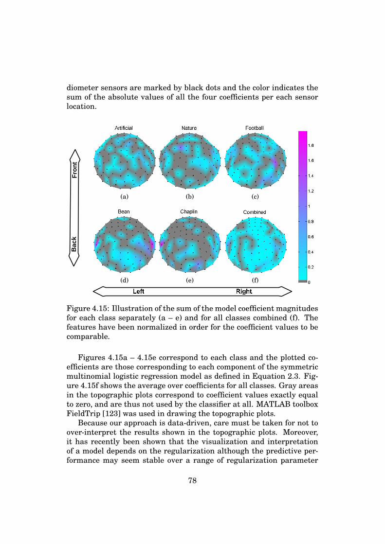
diometer sensors are marked by black dots and the color indicates thesum of the absolute values of all the four coefficients per each sensorlocation.

Bac

kFr

o nt

(a) (b) (c)

(d) (e) (f)

Figure 4.15: Illustration of the sum of the model coefficient magnitudesfor each class separately (a – e) and for all classes combined (f). Thefeatures have been normalized in order for the coefficient values to becomparable.

Figures 4.15a – 4.15e correspond to each class and the plotted co-efficients are those corresponding to each component of the symmetricmultinomial logistic regression model as defined in Equation 2.3. Fig-ure 4.15f shows the average over coefficients for all classes. Gray areasin the topographic plots correspond to coefficient values exactly equalto zero, and are thus not used by the classifier at all. MATLAB toolboxFieldTrip [123] was used in drawing the topographic plots.

Because our approach is data-driven, care must be taken for not toover-interpret the results shown in the topographic plots. Moreover,it has recently been shown that the visualization and interpretationof a model depends on the regularization although the predictive per-formance may seem stable over a range of regularization parameter

78

values [107]. In [21], however, we provide some possible interpreta-tions of the plots and show that a neurologically sensible explanationcan be given to many of the features of the distribution of the coefficientmagnitudes on the topographical plots.

In addition to the multi-class classification case, it is interesting tostudy the problem of classifying between movies with a storyline (Bean,Chaplin) and short video clips with no storyline (Artificial, Nature, andFootball). This can be done by combining classifier outputs correspond-ing to storyline classes as one class and those corresponding to shortclips as another class as was done in the ICANN challenge proceed-ings [105]. In this case, the classification performance of our classifieron the secret test data was 89.7 %. However, a 5-class linear classifierapplied to a 2-class problem in the above manner is not a linear clas-sifier, but a classifier with a piece-wise linear decision surface. Hence,there is a risk that the classifier won’t be regularized enough to achievethe best possible generalization performance for the 2-class case.

As a result of training a binary classifier particularly for the 2-classtask, the classification performance on the secret test data increasesfrom 89.7 % to 96.5 %. This indicates that a simple (linear) classifieris preferred over a more complex classifier (piecewise linear). For sim-plicity, the same initial feature set of mean and detrended standarddeviation and the elastic net mixing parameter α = 0.8 as in the multi-nomial case is used here without further optimization.

Figure 4.16 illustrates the absolute values of the model coefficientsafter feature standardization. As in Figure 4.15, the black nodes markthe locations of the sensors, which are a source of four model coeffi-cients each. Due to the traditional logistic regression model used inthis case (and not the symmetric one) we only have one set of coeffi-cients {β0,β} instead of one set per class. Using the symmetric modelin the 2-class case would result in two identical plots because the co-efficients between the classes only differ by their signs. The figureshows the areas that the classifier uses to discriminate between the twoclasses. As expected, visual comparison indicates some similarities be-tween Figure 4.16 and and corresponding areas in the multi-class casein Figure 4.15f. Further analysis from a neuroscientific point of view isexcluded from this thesis but has been given in [21] for the interested.

79

Bac

kFr

o nt

Figure 4.16: The coefficient magnitudes of a binary classifier trained todistinct movies with a storyline from short clips.

4.5 DiscussionThe previous sections have introduced several real life applicationswhere logistic regression with sparsity promoting coefficient estima-tion has been used. Despite its simple linear structure, the logisticregression classifier has proven to outperform many of the more sophis-ticated methods in classification accuracy. This indicates that many ofthe real life problems are linearly separable, at least with proper fea-ture engineering.

In practical applications, not only is a good classification perfor-mance an essential feature of the method used for classification. Whatalso accounts is computational efficiency and the interpretability of themodel. With the `1 regularized logistic regression model, these areguaranteed by the linearity of the model and recent improvements inthe training algorithms.

Sparse coefficient estimation has proven extremely useful in manyapplications. It enables the embedding of automatic feature selectioninto model training removing the need for explicit feature selection al-gorithms that are often time consuming and don’t necessarily take intoaccount any classifier specific issues that might have an effect on a goodchoice of features. The image segmentation framework introduced inSection 4.1 shows that the feature selection property of the sparse lo-

80

gistic regression classifier is extremely versatile working in differentapplication areas without special knowledge of the application or theneed for major changes into the model, initial set of features, or thelearning algorithms when changing from an application to another.

81

Chapter 5

Conclusions

This thesis has introduced several applications for sparse logistic re-gression classification. The results indicate that this simple linearclassification model together with proper feature engineering and auto-mated feature selection can perform extremely well with various typesof data and applications. From the practical point of view, sparse lo-gistic regression has shown to have several benefits over many otherclassification methods.

One of the main benefits shown for sparse logistic regression is that,with proper choice of the initial set of features, `1 regularized logis-tic regression classifiers can outperform other more complex models inmany different applications. Further, regularization of the `1 norm ofthe coefficient vector results in a sophisticated way to do automatedand computationally efficient feature selection optimized for the linearmodel. Using a simple linear structure of the classifier also helps toavoid overfitting and the coefficients of the linear model are easy tointerpret, which is useful in several applications. Despite this simplelinear structure, top performing results have been attained in real lifeclassification problems, which indicates that these problems are lin-early separable by nature.

From the practical point of view, only one (LASSO) or two (elasticnet) parameters need to be set requiring little effort or expert skillsin training and using the sparse logistic regression model. In addition,recent development in training algorithms allows efficient optimizationof the `1 penalized likelihood function enabling feasible training times.Finally, the logistic regression model is versatile in the sense that itcan be used both with real valued or categorical input data and withbinary or multinomial class labels extending its applicability to manydifferent applications.

82

The application cases where sparse logistic regression classifica-tion has successfully been applied in this thesis consist of diagnosis ofleukemia from flow cytometry data, analysis and classification of brainactivity from MEG data, and supervised image segmentation in twodifferent application fields: object detection in electronics manufactur-ing and spot detection from cell images.

The main results and conclusions for each application case are asfollows:

Image segmentation

• The proposed supervised segmentation framework was shown tooutperform conventional methods both in spot detection from cellimages and in object detection in inkjet printed electronics.

• Logistic regression classification with `1 regularization combinedwith MRF spatial prior was shown to give a better segmentationresult compared to other commonly used classifiers and featureselection algorithms.

• The `1 regularization was shown to work as an efficient featureselector allowing the proposed image segmentation framework towork on multiple application fields without the need for excessparameter tuning or special expertise from the user.

• Additional cost, especially in cell segmentation, is that the newmethod uses training data while conventional methods are usu-ally unsupervised. Our experience, however, is that the trainingstep is rather painless and comparable to tuning of parameters ina corresponding unsupervised method.

• Especially in the inkjet printed electronics case, the new methodwas able to replace multiple processing steps in the image pro-cessing pipeline. This resulted in reduced computation time beingvaluable in a real time application such as computer vision aidedinkjet printed electronics manufacturing.

Diagnosis of AML from flow cytometry data

• Using simple marker mean values as features in an `1 regular-ized logistic regression classifier was shown to produce statisti-cally equal classification results with state-of-the-art methods.

83

• The automatic feature selection property revealed that only 17 ofthe usually measured 49 variables in flow cytometry are actuallyneeded in making the diagnosis.

• Inspecting the coefficient values of the linear model enabled tosort the markers according to their relevance from the viewpointof AML diagnosis. It was found out that the contribution of thethree most significant fluorescence markers to the diagnosis deci-sion is approximately 50 % in terms of absolute coefficient magni-tudes after feature standardization.

Mind reading and analysis from MEG data

• Elastic net regularized logistic regression using detrended meanand standard deviation of the MEG signal as features was shownto outperform several other methods in a multi-class classificationtask.

• The feature selection property of the elastic net regularizationwas able to detect the relevant areas on the skull for each dif-ferent movie type.

• Potentially interesting neuroscientific information can be inferredfrom the relevance of the sensor locations on the skull. However,one should notice that they do not necessarily correspond to theareas with neuroscientifically relevant brain activity.

• With MEG data, it was shown that the elastic net regularizedlogistic regression classifier is rather insensitive to the choice ofthe mixing parameter α.

In addition to experimenting with the logistic regression model, er-ror estimation, especially from the viewpoint of automatic selection ofthe regularization parameter in the `1 penalized classification model,was studied. Results show that, with small sample size, the recentlydeveloped Bayesian error estimator [72, 73] outperforms traditionallyused cross-validation methods both in accuracy and computation time.Generalization of the Bayesian error estimator for multinomial logisticregression is currently under investigation.

Related to model selection, it was shown that conventional methodsfor benchmarking and improving classification models by means of sub-sequent cross-validation runs can lead to unpredictably over-optimistic

84

results. The results are unpredictable in the sense that doing cross-validation by using information from a previous cross-validation runwas, at least in a special case, shown to be more harmful than theclassical mistake of inferring information from all the training databefore the actual cross-validation loop. For instance, conventionallyused sequential feature selection algorithms often use repeated cross-validation to assess the performance of subsequent feature combina-tions. However, the results indicate that even if the cross-validationperformance improves in such a procedure, in reality, the generaliz-ability of the feature set can actually start to decrease at some point.

While the brief experiment in Section 3.2.4 showed that subsequentcross-validation brings optimism into the validation performance, theamount of optimism was not quantified. Thus, we still do not knowhow harmful it exactly is, e.g., to do five subsequent test runs in across-validation test bench and parameter tuning in between in orderto improve our classification model. This is a potential topic for futureresearch.

85

Bibliography

[1] G. Tsoumakas and I. Katakis, “Multi-label classification: Anoverview,” International Journal of Data Warehousing and Min-ing (IJDWM), vol. 3, no. 3, pp. 1–13, 2007.

[2] R. O. Duda, P. E. Hart, and D. G. Stork, Pattern Classification,2nd ed. Wiley-Interscience, 2001.

[3] P. Simon, Too Big to Ignore: The Business Case for Big Data, ser.Wiley and SAS Business Series. Wiley, 2013.

[4] C. Bishop, Pattern Recognition and Machine Learning. Springer,2006, vol. 4.

[5] D. J. Hand, “Classifier technology and the illusion of progress,”Statistical Science, vol. 21, no. 1, pp. 1–14, 2006.

[6] R. A. Fisher, “The use of multiple measurements in taxonomicproblems,” Annals of eugenics, vol. 7, no. 2, pp. 179–188, 1936.

[7] C. Cortes and V. Vapnik, “Support-vector networks,” MachineLearning, vol. 20, no. 3, pp. 273–297, 1995.

[8] S. Press and S. Wilson, “Choosing between logistic regression anddiscriminant analysis,” Journal of the American Statistical Asso-ciation, pp. 699–705, 1978.

[9] T. Hastie, R. Tibshirani, and J. Friedman, The Elements of Statis-tical Learning: Data Mining, Inference, and Prediction, 2nd ed.Springer, 2009.

[10] S. Haykin, Neural networks: a comprehensive foundation. Pren-tice Hall PTR, 1994.

[11] P. MacCullagh and J. A. Nelder, Generalized linear models. CRCpress, 1989, vol. 37.

86

[12] J.-H. Xue and D. M. Titterington, “Comment on ”On discrimina-tive vs. generative classifiers: A comparison of logistic regressionand naive Bayes”,” Neural processing letters, vol. 28, no. 3, pp.169–187, 2008.

[13] B. Efron, “The efficiency of logistic regression compared to nor-mal discriminant analysis,” Journal of the American StatisticalAssociation, vol. 70, no. 352, pp. 892–898, 1975.

[14] A. Y. Ng and M. I. Jordan, “On discriminative vs. generativeclassifiers: A comparison of logistic regression and naive Bayes,”in Advances in Neural Information Processing Systems 14: Pro-ceedings of the 2001 Conference, Z. G. Thomas Glen Dietterich,Suzanna Becker, Ed. MIT Press, 2002, pp. 841–848.

[15] T. J. O’Neill, “The general distribution of the error rate of a classi-fication procedure with application to logistic regression discrim-ination,” Journal of the American Statistical Association, vol. 75,no. 369, pp. 154–160, 1980.

[16] Y. D. Rubinstein, T. Hastie et al., “Discriminative vs informativelearning,” in KDD, vol. 5, 1997, pp. 49–53.

[17] D. Titterington, G. Murray, L. Murray, D. Spiegelhalter,A. Skene, J. Habbema, and G. Gelpke, “Comparison of discrimi-nation techniques applied to a complex data set of head injuredpatients,” Journal of the Royal Statistical Society. Series A (Gen-eral), pp. 145–175, 1981.

[18] T. Manninen, H. Huttunen, P. Ruusuvuori, and M. Nykter,“Leukemia prediction using sparse logistic regression,” PLoSONE, vol. 8, no. 8, p. e72932, Aug. 2013.

[19] T. Manninen, V. Pekkanen, K. Rutanen, P. Ruusuvuori,R. Rönkkä, and H. Huttunen, “Alignment of individually adaptedprint patterns for ink jet printed electronics,” Journal of ImagingScience and Technology, vol. 54, no. 5, p. 050306, 2010.

[20] P. Ruusuvuori, T. Manninen, and H. Huttunen, “Image segmen-tation using sparse logistic regression with spatial prior,” in Sig-nal Processing Conference (EUSIPCO), 2012 Proceedings of the20th European, Aug. 2012, pp. 2253–2257.

87

[21] H. Huttunen, T. Manninen, J.-P. Kauppi, and J. Tohka, “Mindreading with regularized multinomial logistic regression,” Ma-chine Vision and Applications, vol. 24, no. 6, pp. 1311–1325,2013.

[22] H. Huttunen, T. Manninen, and J. Tohka, “MEG mind reading:Strategies for feature selection,” in Proceedings of the FederatedComputer Science Event 2012, 2012, pp. 42–49.

[23] ——, “Bayesian error estimation and model selection in sparselogistic regression,” in 2013 IEEE International Workshop onMachine Learning for Signal Processing, MLSP2013, Southamp-ton, UK, Sep. 2013.

[24] J. Cramer, “The origins of logistic regression,” Tinbergen Insti-tute, Tinbergen Institute Discussion Papers 02-119/4, Dec. 2002.

[25] G. Cawley and N. Talbot, “Gene selection in cancer classificationusing sparse logistic regression with Bayesian regularization,”Bioinformatics, vol. 22, no. 19, pp. 2348–2355, 2006.

[26] J. H. Friedman, T. Hastie, and R. Tibshirani, “Regularizationpaths for generalized linear models via coordinate descent,” Jour-nal of Statistical Software, vol. 33, no. 1, pp. 1–22, 2010.

[27] J. E. Griffin and P. J. Brown, “Bayesian hyper-Lassos with non-convex penalization,” Australian & New Zealand Journal ofStatistics, vol. 53, no. 4, pp. 423–442, 2011.

[28] H. Zou and T. Hastie, “Regularization and variable selection viathe elastic net,” Journal of the Royal Statistical Society: Series B(Statistical Methodology), vol. 67, no. 2, pp. 301–320, 2005.

[29] A. Webb, Statistical Pattern Recognition, 2nd ed. John Wileyand Sons Ltd., 2002.

[30] D. C. Liu and J. Nocedal, “On the limited memory BFGS methodfor large scale optimization,” Mathematical Programming,vol. 45, no. 1–3, pp. 503–528, 1989. [Online]. Available:http://dx.doi.org/10.1007/BF01589116

[31] P. J. Green, “Iteratively reweighted least squares for maximumlikelihood estimation, and some robust and resistant alterna-tives,” Journal of the Royal Statistical Society. Series B (Method-ological), pp. 149–192, 1984.

88

[32] D. Rubin, “Iteratively reweighted least squares,” Encyclopedia ofstatistical sciences, vol. 4, pp. 272–275, 1983.

[33] P. Peduzzi, J. Concato, E. Kemper, T. R. Holford, and A. R. Fein-stein, “A simulation study of the number of events per variablein logistic regression analysis,” Journal of clinical epidemiology,vol. 49, no. 12, pp. 1373–1379, 1996.

[34] R. Tibshirani, “Regression shrinkage and selection via the lasso,”Journal of the Royal Statistical Society. Series B (Methodologi-cal), pp. 267–288, 1996.

[35] S. S. Chen, D. L. Donoho, and M. A. Saunders, “Atomic decom-position by basis pursuit,” SIAM journal on scientific computing,vol. 20, no. 1, pp. 33–61, 1998.

[36] A. Hoerl and R. Kennard, “Ridge regression: Biased estimationfor nonorthogonal problems,” Technometrics, pp. 55–67, 1970.

[37] A. Y. Ng, “Feature selection, L1 vs. L2 regularization, and rota-tional invariance,” in Proceedings of the twenty-first internationalconference on Machine learning. ACM, 2004, p. 78.

[38] B. Krishnapuram, L. Carin, M. Figueiredo, and A. Hartemink,“Sparse multinomial logistic regression: fast algorithms and gen-eralization bounds,” Pattern Analysis and Machine Intelligence,IEEE Transactions on, vol. 27, no. 6, pp. 957–968, Jun. 2005.

[39] A. Genkin, D. Lewis, and D. Madigan, “Large-scale Bayesian lo-gistic regression for text categorization,” Technometrics, vol. 49,no. 3, pp. 291–304, 2007.

[40] S. Shevade and S. Keerthi, “A simple and efficient algorithm forgene selection using sparse logistic regression,” Bioinformatics,vol. 19, no. 17, pp. 2246–2253, 2003.

[41] S. Raman and V. Roth, “Sparse Bayesian regression for groupedvariables in generalized linear models,” in Pattern Recognition,ser. Lecture Notes in Computer Science, J. Denzler, G. Notni, andH. Süße, Eds. Springer Berlin / Heidelberg, 2009, vol. 5748, pp.242–251.

[42] D. F. Andrews and C. L. Mallows, “Scale mixtures of normaldistributions,” Journal of the Royal Statistical Society. Series B(Methodological), pp. 99–102, 1974.

89

[43] M. A. Figueiredo, “Adaptive sparseness for supervised learning,”Pattern Analysis and Machine Intelligence, IEEE Transactionson, vol. 25, no. 9, pp. 1150–1159, 2003.

[44] C. Ambroise and G. McLachlan, “Selection bias in gene extrac-tion on the basis of microarray gene-expression data,” Proceed-ings of the National Academy of Sciences, vol. 99, no. 10, p. 6562,2002.

[45] F. Caron and A. Doucet, “Sparse Bayesian nonparametric regres-sion,” in Proceedings of the 25th international conference on Ma-chine learning. ACM, 2008, pp. 88–95.

[46] T. Virtanen, R. Singh, and B. Raj, Techniques for Noise Robust-ness in Automatic Speech Recognition. Wiley, 2012.

[47] K. Binder, “Ising model,” Encyclopedia of Mathematics, 2011,uRL: http://www.encyclopediaofmath.org/index.php?title=Ising_model&oldid=15668.

[48] S. Li, Markov Random Field Modeling in Image Analysis, 3rd ed.,ser. Advances in Computer Vision and Pattern Recognition.Springer, 2009.

[49] E. Ising, “Beitrag zur theorie des ferromagnetismus,” Zeitschriftfür Physik A Hadrons and Nuclei, vol. 31, no. 1, pp. 253–258,1925.

[50] S. Geman and D. Geman, “Stochastic relaxation, Gibbs distribu-tions, and the Bayesian restoration of images,” Pattern Analysisand Machine Intelligence, IEEE Transactions on, vol. 6, no. 6, pp.721–741, Nov. 1984.

[51] J. Borges, J. Bioucas-Dias, and A. Marcal, “Bayesian hyper-spectral image segmentation with discriminative class learning,”Geoscience and Remote Sensing, IEEE Transactions on, vol. 49,no. 6, pp. 2151–2164, Jun. 2011.

[52] D. M. Greig, B. T. Porteous, and A. H. Seheult, “Exact maximuma posteriori estimation for binary images,” Journal of the RoyalStatistical Society., vol. 51, no. 2, pp. 271–279, 1989.

[53] Y. Boykov and V. Kolmogorov, “An experimental comparison ofmin-cut/max-flow algorithms for energy minimization in vision,”

90

Pattern Analysis and Machine Intelligence, IEEE Transactionson, vol. 26, no. 9, pp. 1124–1137, Sep. 2004.

[54] M. Sokolova and G. Lapalme, “A systematic analysis of perfor-mance measures for classification tasks,” Information Processing& Management, vol. 45, no. 4, pp. 427–437, 2009.

[55] D. D. Lewis, “Evaluating text categorization i.” in HLT, vol. 91,1991, pp. 312–318.

[56] G. Tsoumakas and I. Vlahavas, “Random k-labelsets: An ensem-ble method for multilabel classification,” in Machine Learning:ECML 2007. Springer, 2007, pp. 406–417.

[57] Y. Yang, “An evaluation of statistical approaches to text catego-rization,” Information Retrieval, vol. 1, no. 1–2, pp. 69–90, 1999.

[58] C. E. Metz, “Basic principles of ROC analysis,” Seminars in Nu-clear Medicine, vol. 8, no. 4, pp. 283–298, 1978.

[59] T. Fawcett, “An introduction to ROC analysis,” Pattern recogni-tion letters, vol. 27, no. 8, pp. 861–874, 2006.

[60] A. P. Bradley, “The use of the area under the ROC curve in theevaluation of machine learning algorithms,” Pattern recognition,vol. 30, no. 7, pp. 1145–1159, 1997.

[61] J. A. Hanley and B. J. McNeil, “The meaning and use of the areaunder a receiver operating characteristic (ROC) curve,” Radiol-ogy, vol. 143, no. 1, pp. 29–36, Apr. 1982.

[62] D. J. Hand and R. J. Till, “A simple generalisation of the areaunder the ROC curve for multiple class classification problems,”Machine Learning, vol. 45, no. 2, pp. 171–186, 2001.

[63] T. C. Landgrebe and R. P. Duin, “Approximating the multiclassROC by pairwise analysis,” Pattern recognition letters, vol. 28,no. 13, pp. 1747–1758, 2007.

[64] C. Sima, U. Braga-Neto, and E. R. Dougherty, “Superior feature-set ranking for small samples using bolstered error estimation,”Bioinformatics, vol. 21, no. 7, pp. 1046–1054, 2005.

[65] V. N. Vapnik, Statistical learning theory. Wiley, 1998.

91

[66] B. Efron, “Bootstrap methods: another look at the jackknife,” Theannals of Statistics, pp. 1–26, 1979.

[67] ——, “Estimating the error rate of a prediction rule: Improve-ment on cross-validation,” Journal of the American StatisticalAssociation, vol. 78, no. 382, pp. 316–331, 1983.

[68] U. M. Braga-Neto and E. R. Dougherty, “Is cross-validationvalid for small-sample microarray classification?” Bioinformat-ics, vol. 20, no. 3, pp. 374–380, 2004.

[69] H. Akaike, “A new look at the statistical model identification,”Automatic Control, IEEE Transactions on, vol. 19, no. 6, pp. 716–723, 1974.

[70] G. Schwarz, “Estimating the dimension of a model,” The annalsof statistics, vol. 6, no. 2, pp. 461–464, 1978.

[71] J. Chen and Z. Chen, “Extended BIC for small-n-large-P sparseGLM,” Statistica Sinica, vol. 22, no. 2, p. 555, 2012.

[72] L. Dalton and E. Dougherty, “Bayesian minimum mean-squareerror estimation for classification error — part I: Definition andthe Bayesian MMSE error estimator for discrete classification,”Signal Processing, IEEE Transactions on, vol. 59, no. 1, pp. 115–129, 2011.

[73] ——, “Bayesian minimum mean-square error estimation for clas-sification error — part II: Linear classification of Gaussian mod-els,” Signal Processing, IEEE Transactions on, vol. 59, no. 1, pp.130–144, 2011.

[74] P. Pudil, J. Novovicová, and J. Kittler, “Floating search methodsin feature selection,” Pattern Recogn. Lett., vol. 15, no. 11, pp.1119–1125, Nov. 1994.

[75] J.-C. Olivo-Marin, “Extraction of spots in biological images us-ing multiscale products,” Pattern Recognition, vol. 35, no. 9, pp.1989–1996, 2002.

[76] T. Ojala, M. Pietikainen, and T. Maenpaa, “Multiresolution gray-scale and rotation invariant texture classification with local bi-nary patterns,” IEEE Transactions on Pattern Analysis and Ma-chine Intelligence, vol. 24, no. 7, pp. 971–987, 2002.

92

[77] J. Li, “Discriminative image segmentation: Applications to hy-perspectral data,” Ph.D. dissertation, Universidade Tecnica DeLisboa, 2011.

[78] P. Paclik, R. Duin, G. van Kempen, and R. Kohlus, “Super-vised segmentation of textures in backscatter images,” in Pat-tern Recognition, 2002. Proceedings. 16th International Confer-ence on, vol. 2, 2002, pp. 490–493.

[79] S. Kumar and M. Hebert, “Discriminative random fields,” Inter-national Journal of Computer Vision, vol. 68, no. 2, pp. 179–201,2006.

[80] M. Farhan, P. Ruusuvuori, M. Emmenlauer, P. Rämö, C. De-hio, and O. Yli-Harja, “Multi-scale Gaussian representation andoutline-learning based cell image segmentation,” BMC Bioinfor-matics, vol. 14, no. 10, pp. 1–14, 2013.

[81] P. Ruusuvuori, T. Äijö, S. Chowdhury, C. Garmendia-Torres,J. Selinummi, M. Birbaumer, A. Dudley, L. Pelkmans, and O. Yli-Harja, “Evaluation of methods for detection of fluorescence la-beled subcellular objects in microscope images.” BMC Bioinfor-matics, vol. 11, p. 248, 2010.

[82] P. Ruusuvuori, A. Lehmussola, J. Selinummi, T. Rajala, H. Hut-tunen, and O. Yli-Harja, “Benchmark set of synthetic images forvalidating cell image analysis algorithms,” in Proceedings of the16th European Signal Processing Conference. EUSIPCO, 2008.

[83] J. Miettinen, V. Pekkanen, K. Kaija, P. Mansikkamäki, J. Män-tysalo, M. Mäntysalo, J. Niittynen, J. Pekkanen, T. Saviauk, andR. Rönkkä, “Inkjet printed system-in-package design and manu-facturing,” Elsevier Microelectr. J., 2008.

[84] K. Kaija, V. Pekkanen, M. Mäntysalo, and P. Mansikkamäki,“Controlling warpage of molded package for inkjet manufactur-ing,” Microelectronic Engineering, vol. 85, no. 3, pp. 518–526,2008.

[85] M. Moganti, F. Ercal, C. Dagli, and S. Tsunekawa, “AutomaticPCB inspection algorithms: A survey,” Computer Vision and Im-age Processing, vol. 63, pp. 287–313, Mar. 1996.

93

[86] J. C. Gower and G. B. Dijksterhuis, Procrustes problems. OxfordUniversity Press Oxford, 2004, vol. 3.

[87] T. Manninen, R. Rönkkä, and H. Huttunen, “Point patternmatching for 2-D point sets with regular structure,” in ImageAnalysis, ser. Lecture Notes in Computer Science, A. Heyden andF. Kahl, Eds. Springer Berlin / Heidelberg, 2011, vol. 6688, pp.156–165.

[88] H. Huttunen, T. Manninen, K. Rutanen, P. Ruusuvuori, R. Mäki-nen, and R. Rönkkä, “Dynamic correction of interconnections inprinted electronics manufacturing,” in International conferenceon digital printing technologies, NIP25, Louisville, Kentucky,USA, Sep. 2009, pp. 589–592.

[89] H. Huttunen, P. Ruusuvuori, T. Manninen, K. Rutanen,R. Rönkkä, and A. Visa, “Object detection for dynamic adaptationof interconnections in inkjet printed electronics,” in 15th IEEEInternational Conference on Image Processing, ICIP 2008, SanDiego, California, USA, Oct. 2008, pp. 2364–2367.

[90] M. Kamel and A. Zhao, “Extraction of binary character/graphicsimages from grayscale document images,” CVGIP: GraphicalModels and Image Processing, vol. 55, no. 3, pp. 203–217, 1993.

[91] T. Manninen, H. Huttunen, P. Ruusuvuori, and M. Nykter, “Lo-gistic regression for AML prediction,” in Dialogue for ReverseEngineering Assessments and Methods, DREAM6, Barcelona,Spain, Oct. 2011.

[92] N. Aghaeepour, G. Finak, The Flowcap Consortium, The DREAMConsortium, H. Hoos, T. R. Mosmann, R. Gottardo, R. R.Brinkman, and R. H. Scheuermann, “Critical assessment of au-tomated flow cytometry data analysis techniques,” Nature meth-ods, vol. 10, no. 3, pp. 228–238, 2013.

[93] T. Willis and M. Dyer, “The role of immunoglobulin transloca-tions in the pathogenesis of B-cell malignancies,” Blood, vol. 96,no. 3, pp. 808–822, 2000.

[94] J. Vardiman, N. Harris, and R. Brunning, “The world healthorganization (WHO) classification of the myeloid neoplasms,”Blood, vol. 100, no. 7, pp. 2292–2302, 2002.

94

[95] G. Henel and J. L. Schmitz, “Basic theory and clinical applica-tions of flow cytometry,” Lab Med, vol. 38, no. 7, pp. 428–436,2007.

[96] E. Lugli, M. Roederer, and A. Cossarizza, “Data analysis in flowcytometry: The future just started,” Cytometry A, vol. 77, no. 7,pp. 705–713, 2010.

[97] D. R. Parks, M. Roederer, and W. A. Moore, “A new ”logicle” dis-play method avoids deceptive effects of logarithmic scaling forlow signals and compensated data,” Cytometry A, vol. 69, no. 6,pp. 541–551, Jun. 2006.

[98] T. A. Knijnenburg, O. Roda, Y. Wan, G. P. Nolan, J. D. Aitchison,and I. Shmulevich, “A regression model approach to enable cellmorphology correction in high-throughput flow cytometry,” MolSyst Biol, vol. 7, p. 531, 2011.

[99] T. W. Anderson, “On the distribution of the two-sample Cramér-von Mises criterion,” Ann Math Statist, vol. 33, no. 3, pp. 1148–1159, 1962.

[100] F. J. Massey, “The Kolmogorov-Smirnov test for goodness of fit,”J Am Statist Assoc, vol. 46, no. 253, pp. 68–78, 1951.

[101] S. Kullback and R. A. Leibler, “On information and sufficiency,”Ann Math Statist, vol. 22, no. 1, pp. 79–86, 1951.

[102] M. Biehl, K. Bunte, and P. Schneider, “Analysis of flow cytometrydata by matrix relevance learning vector quantization,” PLoSOne, vol. 8, no. 3, p. e59401, Mar. 2013.

[103] I. Vergara, T. Norambuena, E. Ferrada, A. Slater, and F. Melo,“StAR: a simple tool for the statistical comparison of ROCcurves,” BMC Bioinformatics, vol. 9, no. 1, p. 265, 2008.

[104] R. C. Holte, “Very simple classification rules perform well onmost commonly used datasets,” Machine learning, vol. 11, no. 1,pp. 63–90, 1993.

[105] A. Klami, P. Ramkumar, S. Virtanen, L. Parkkonen, R. Hari,and S. Kaski, “ICANN/PASCAL2 Challenge: MEG Mind-Reading — Overview and Results,” 2011. [Online]. Available:http://www.cis.hut.fi/icann2011/meg/megicann_proceedings.pdf

95

[106] D. van De Ville and S.-W. Lee, “Brain decoding: Opportuni-ties and challenges for pattern recognition,” Pattern Recognition,Special Issue on Brain Decoding, vol. 45, no. 6, pp. 2033 – 2034,2012.

[107] P. M. Rasmussen, L. K. Hansen, K. H. Madsen, N. W. Churchill,and S. C. Strother, “Model sparsity and brain pattern interpreta-tion of classification models in neuroimaging,” Pattern Recogni-tion, vol. 45, no. 6, pp. 2085–2100, 2012.

[108] T. Naselaris, K. N. Kay, S. Nishimoto, and J. L. Gallant, “En-coding and decoding in fMRI,” NeuroImage, vol. 56, no. 2, pp.400–410, 2011.

[109] F. Pereira, T. Mitchell, and M. Botvinick, “Machine learning clas-sifiers and fMRI: a tutorial overview,” NeuroImage, vol. 45, no.Suppl 1, pp. S199 – S209, 2009.

[110] A. J. O’Toole, F. Jiang, H. Abdi, N. Pénard, J. P. Dunlop, and M. A.Parent, “Theoretical, statistical, and practical perspectives onpattern-based classification approaches to the analysis of func-tional neuroimaging data,” Journal of Cognitive Neuroscience,vol. 19, no. 11, pp. 1735–1752, 2007.

[111] B. Blankertz, M. Tangermann, C. Vidaurre, S. Fazli, C. Sannelli,S. Haufe, C. Maeder, L. Ramsey, I. Sturm, G. Curio, and K.-R. Müller, “The Berlin Brain-Computer Interface: Non-medicaluses of BCI technology,” Front Neurosci, vol. 4, p. 198, 2010.

[112] B. Blankertz, K.-R. Müller, D. J. Krusienski, G. Schalk, J. R. Wol-paw, A. Schlögl, G. Pfurtscheller, J. del R Millán, M. Schröder,and N. Birbaumer, “The BCI competition III: Validating alter-native approaches to actual BCI problems,” IEEE Trans NeuralSyst Rehabil Eng, vol. 14, no. 2, pp. 153–159, Jun. 2006.

[113] M. van Gerven, C. Hesse, O. Jensen, and T. Heskes, “Interpretingsingle trial data using groupwise regularisation,” Neuroimage,vol. 46, pp. 665 – 676, 2009.

[114] R. Tomioka and K.-R. Müller, “A regularized discriminativeframework for EEG analysis with application to brain-computerinterface,” NeuroImage, vol. 49, no. 1, pp. 415–432, 2010.

96

[115] M. Tangermann, K.-R. Müller, A. Aertsen, N. Birbaumer,C. Braun, C. Brunner, R. Leeb, C. Mehring, K. J. Miller,G. Mueller-Putz, G. Nolte, G. Pfurtscheller, H. Preissl, G. Schalk,A. Schlögl, C. Vidaurre, S. Waldert, and B. Blankertz, “Reviewof the BCI competition IV,” Frontiers in Neuroscience, vol. 6, no.00055, 2012.

[116] A. Zhdanov, T. Hendler, L. Ungerleider, and N. Intrator, “Infer-ring functional brain states using temporal evolution of regular-ized classifiers,” Comput Intell Neurosci, p. 52609, 2007.

[117] A. M. Chan, E. Halgren, K. Marinkovic, and S. S. Cash, “Decod-ing word and category-specific spatiotemporal representationsfrom MEG and EEG,” Neuroimage, vol. 54, no. 4, pp. 3028–3039,Feb. 2011.

[118] J. W. Rieger, C. Reichert, K. R. Gegenfurtner, T. Noesselt,C. Braun, H.-J. Heinze, R. Kruse, and H. Hinrichs, “Predictingthe recognition of natural scenes from single trial MEG record-ings of brain activity,” Neuroimage, vol. 42, no. 3, pp. 1056–1068,Sep. 2008.

[119] M. Besserve, K. Jerbi, F. Laurent, S. Baillet, J. Martinerie, andL. Garnero, “Classification methods for ongoing EEG and MEGsignals,” Biol Res, vol. 40, no. 4, pp. 415–437, 2007.

[120] L. Grosenick, S. Greer, and B. Knutson, “Interpretable classifiersfor FMRI improve prediction of purchases,” IEEE Trans NeuralSyst Rehabil Eng, vol. 16, no. 6, pp. 539–548, Dec. 2008.

[121] M. K. Carroll, G. A. Cecchi, I. Rish, R. Garg, and A. R. Rao,“Prediction and interpretation of distributed neural activity withsparse models,” Neuroimage, vol. 44, no. 1, pp. 112–122, Jan.2009.

[122] S.-W. Lin, Z.-J. Lee, S.-C. Chen, and T.-Y. Tseng, “Parameter de-termination of support vector machine and feature selection us-ing simulated annealing approach,” Appl. Soft Comput., vol. 8,pp. 1505–1512, 2008.

[123] R. Oostenveld, P. Fries, E. Maris, and J.-M. Schoffelen, “Field-trip: open source software for advanced analysis of MEG, EEG,and invasive electrophysiological data,” Intell. Neuroscience, vol.2011, pp. 1:1–1:9, Jan. 2011.

97