predictive macro-finance with dynamic partition...

Predictive Macro-Finance With DynamicPartition Models

Daniel ZANTEDESCHI, Paul DAMIEN, and Nicholas G. POLSON

Dynamic partition models are used to predict movements in the term structure of interest rates. This allows one to understand historic cyclesin the performance of how interest rates behave, and to offer policy makers guidance regarding future expectations on their evolution. Ourapproach allows for a random number of possible change points in the term structure of interest rates. We use particle learning to learnabout the unobserved state variables in a new class of dynamic product partition models that relate macro-variables to term structures. Theempirical results, using data from 1970 to 2000, clearly identifies some of the key shocks to the economy, such as recessions. We constructa time series of Bayes factors that, surprisingly, could serve as a leading indicator of economic activity, validated via a Granger causalitytest. Finally, the in-sample and out-of-sample forecasts from our model are quite robust regardless of the time to maturity of interest rates.

KEY WORDS: Bayes factor; Bond yield; Nelson–Siegel model; Particle learning.

1. INTRODUCTION

The recent economic crisis has brought into focus the im-portance of having sound methods to understand the behaviorof financial and macro-economic time series. We use the term“predictive macro-finance” to describe statistical models thatuse macro-economic variables to predict financial asset returns.Understanding the term structure, or yield curves, of differentbond maturities has a long history. Recently the Nelson–Siegel(1987) yield curve model (N–S) has been rekindled by a se-ries of articles showing superior predictive performance overtraditional models. The articles of Diebold and Li (2006) andDiebold, Rudebusch, and Aruoba (2006) highlight the three fac-tor N–S model as a powerful tool for forecasting changes inrates. These authors showed that their model-based forecastsoutperform many of the standard models. Koopman, Mallee,and van der Wel (2010) used a time-varying loadings version toachieve further gains.

We extend the dynamic N–S approach in a number of ways.First, we propose a dynamic product partition model (PPM)to allow for an unknown number of change points. This ad-dresses one of the fundamental challenges in yield curve mod-eling where parameter shifts occur for various reasons, eitherpolicy-induced (e.g., the Volcker period of the early 1980s) orpurely probabilistic (e.g., the 1995 change point reported inChib and Kang 2009). Our approach incorporates both of theseeffects. Second, we develop a particle learning strategy to learnabout the unobserved state variables and parameters. Third, ourempirical results identify many of the key shocks (e.g., reces-sions, expansions) to the economy. We quantify the gains fromour extensions from both in-sample fit and out-of-sample fore-cast perspectives. We also show that our results are robust tothe maturity of interest rates. Finally, and most importantly, weconstruct a time series of regime diagnostics based on Bayesfactors that can serve as a leading indicator of economic activ-ity, validated via a Granger causality test.

Daniel Zantedeschi is Graduate Researcher (E-mail: [email protected]) and Paul Damien is Professor (E-mail: [email protected]), McCombs School of Business, University of Texasat Austin, 1 University Station B6000, Austin, TX 78712. Nicholas G.Polson is Professor, Booth School of Business, University of Chicago, 5807South Woodlawn Avenue, Chicago, IL 60637 (E-mail: [email protected]).

Fama (2006) observed that if spot rates are subject to severalpermanent shocks to the system, then limiting the number ofregime changes up front to two or three may prove inadequateto explain the data. Our approach addresses this by allowing fora possible regime change at every time point, and our analy-sis assesses the posterior probability of possible change pointsgiven the dynamic N–S term structure model. Two alternativeapproaches include those of Sims and Zha (1998, 2006), whomodeled regime switches in U.S. monetary policy with a fixednumber of (at most nine) regimes. Chib and Kang (2009) usedup to four change points by exploiting a transient parameteriza-tion of a hidden Markov Model.

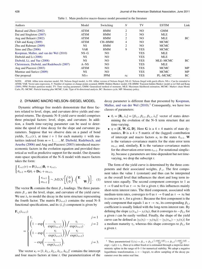
One challenging issue when fitting dynamic state-space mod-els with a random number of change points is the computa-tional explosion of the number of possible models. We arguethat PPMs (Barry and Hartigan 1992, 1993), when coupled withparticle learning methods, bypass this dilemma. Our approachalso calculates a sequential Bayes factor at each time point formodel comparison. We thus allow for multiple, random changepoints—a first in the macro-finance context. Table 1 comparesour approach with that of competing models in the literature.

Explaining the cross-section of rates has traditionally beenachieved with affine term-structure models (ATSMs; see, e.g.,Chib and Ergashev 2009). Theoretically, these models are verypopular because of their arbitrage-free properties; however,they have suffered somewhat in out-of-sample time series pre-diction exercises (see, e.g., Duffee 2002). The Bank of Interna-tional Settlements (2005) reported that 9 out of 13 central banksthat report their term structure modeling results to the BIS usethe N–S model (or some minor variation thereof) rather thanATSMs to estimate yield curves.

The rest of the article is organized as follows. Section 2provides a general framework for term structure models withmacro-economic factors using the N–S model. Section 3 showshow to extend these models to allow for multiple change pointsin the form of a PPM. Section 4 details the term structure andmacro-finance monthly data for 1970–2000 used in this study,which is used in Section 5 to carry out a comprehensive analy-sis. Section 6 concludes.

© 2011 American Statistical AssociationJournal of the American Statistical Association

June 2011, Vol. 106, No. 494, Applications and Case StudiesDOI: 10.1198/jasa.2011.ap09732

427

mailto:[email protected]



http://www.amstat.org

http://pubs.amstat.org/loi/jasa

http://dx.doi.org/10.1198/jasa.2011.ap09732




428 Journal of the American Statistical Association, June 2011

Table 1. Main predictive macro-finance model presented in the literature

Authors Model Switching N TV ESTIM Link

Bansal and Zhou (2002) ATSM HMM 2 NO GMMDai and Singleton (2007) ATSM HMM 2 NO MLEAng and Bekaert (2002) ATSM HMM 2 NO MLE BCChib and Kang (2009) ATSM CH–HMM 4 NO MCMCZhu and Rahman (2009) NS HMM 2 NO MCMCSims and Zha (2006) VAR HMM 9 YES MCMCKoopman, Mallee, and van der Wel (2010) NS–G NO YES MLEDiebold and Li (2006) NS NO YES MLEDiebold, Li, and Yue (2008) NS NO YES MLE–MCMC BCChristensen, Diebold, and Rudebusch (2007) A–NS NO YES MLEAng and Piazzesi (2003) ATSM NO YES MCMC MPMumtaz and Surico (2009) NS NO YES MCMC MPOur proposal NS+ PPM ∞ YES PL–MCMC BC

NOTE: ATSM: Affine term structure model, NS: Nelson–Siegel model, A–NS: Affine version of Nelson–Siegel, NS–G: Nelson–Siegel with garch effects, NS+: Can be extended toATSM, VAR: Vector auto-regression, N: Number of regimes or change points assumed, HMM: Hidden Markov model, CH–HMM: Transient hidden Markov model as in Chib and Kang(2009), PPM: Product partition model, TV: Time varying parameters, GMM: Generalized method of moments, MLE: Maximum likelihood estimation, MCMC: Markov chain MonteCarlo, PL–MCMC: Particle learning plus MCMC, Link: Type of bi-directional analysis, BC: Business cycle, MP: Monetary policy.

2. DYNAMIC MACRO NELSON–SIEGEL MODEL

Dynamic arbitrage free models demonstrate that three fac-tors related to level, slope, and curvature drive yields and one-period returns. The dynamic N–S yield curve model comprisesthree principal factors: level, slope, and curvature. In addi-tion, a fourth time-varying parameter can be used to deter-mine the speed of time decay for the slope and curvature pa-rameters. Suppose that we observe data on a panel of bondyields, Yt+1(τ ), at time t + 1 for each maturity τ with ma-turities indexed from m = 1, . . . ,M. Diebold, Rudebusch, andAruoba (2006) and Ang and Piazzesi (2003) introduced macro-economic factors in the evolution equation and provided theo-retical as well as predictive support for the model. Our dynamicstate-space specification of the N–S model with macro factorstakes the form:{

Yt+1(τ ) = F(λt+1)Bt + εt+1,

θt+1 = Gθt + Dκt + ωt+1,{εt+1ωt+1

}∼ M V N

[(00

),

(E

W

)]. (1)

The vector Bt contains the three β·,t loadings. The three param-eters β·,t are the level, slope, and curvature of the yield curve.We use λt to model the decay in the term structure representingthe fourth factor. The matrix F(λt+1) contains the usual N–Sfunctional specifications, and its (i, j) component is given by

Fi,j(λt+1)

=

⎧⎪⎪⎪⎪⎪⎪⎪⎪⎪⎨⎪⎪⎪⎪⎪⎪⎪⎪⎪⎩

1, j = 1(1 − exp

(− τi

exp(λt+1)

))/ τi

exp(λt+1), j = 2(

1 − exp

(− τi

exp(λt+1)

))/ τi

exp(λt+1)

− exp

(− τi

exp(λt+1)

), j = 3.

The vector κt = [1, k1,t, k2,t, k3,t, k4,t]′ contains the interceptand four macro factors at time t. Our parameterization of the

decay parameter is different than that presented by Koopman,Mallee, and van der Wel (2010).1 Consequently, we have twoclasses of parameters:

• θt = [Bt, λt] = [β1,t, β2,t, β3,t, λt]′ vector of states deter-mining the evolution of the N–S term structure that aretime-varying.

• η = [E,W,G,D]. Here G is a 4 × 4 matrix of state dy-namics, D is a 4 × 5 matrix of the (lagged) contributionof intercept and macro factors κt to the states θt+1. Wis the variance–covariance matrix for the state error termωt+1 and, similarly, E is the variance–covariance matrixfor the observation error term εt+1. For notational simplic-ity, because η parameters are time-dependent but not time-varying, we drop the subscript t.

The form of the yield curve is determined by the three com-ponents and their associated weights, β·,t. The first compo-nent takes the value 1 (constant) and thus can be interpretedas the overall level that influences the short and long term in-terest rates equally. The second component converges to 1 asτ → 0 and to 0 as τ → ∞ for a given t; this influences mainlyshort-term interest rates. The third component, associated withmedium-term rates, converges to 0 as τ → 0 and as τ → ∞ butis concave in τ , for a given t. Because the first component is theonly component that equals 1 as τ → ∞, its corresponding β1,t

coefficient is usually linked with the long-term interest rate. Bydefining the slope yt(τ∞)− yt(τ0), that it converges to −β2,t fora given t can be easily verified. Finally, the shape of the yieldcurve can be defined as |yt(τi) − yt(τ0)| − |yt(τ∞) − yt(τi)| fora medium maturity τi, whereas this shape converges to β3,t fora given t.

1 They parameterized Yt(τi) = β1,t + β2,t(1−exp(−τiφ)

τiφ) + β3,t(

1−exp(−τiφ)

τiφ−

exp(−τiφ))+εt . Here φ is either fixed or is estimated through a stepwise deter-ministic spline in the range of 0–1 for numerical stability. We adopt a negativelogarithmic transformation, λ = − log(φ), to allow sampling of the decay pa-rameter over the entire real line.

Zantedeschi, Damien, and Polson: Predictive Macro-Finance 429

3. DYNAMIC PARTITION MODELS

PPMs were introduced by Barry and Hartigan (1992, 1993)as a clustering device producing time-inhomogenous time se-ries. Barry and Hartigan articulated the following key idea:These [PPM] models apply with special computational simplicity to changepoint problems, where the partitions divide the sequence of observations intocomponents within which different regimes hold . . . [and] that the observationscan eventually determine approximately the true partition.

Let Y = (y1, . . . ,yT) be a time series that we wish topartition into B contiguous segments defined by {1, . . . , t1},{t1 + 1, . . . , t2}, {tB−1, . . . ,T} with t1, t2, . . . , tB−1 denoting thechange points. Equivalently, we can use a T-dimensional setof binary indicators, U = (1,u2, . . . ,uT−1,1)′, with the eventut = 1 implying a change point and ut = 0 implying no changepoint.

PPMs use a random number of segments B obtained via apartition ρ ≡ (1, t1, . . . , tB−1,T), which divides the data Y intoB contiguous blocks, denoted by Ytr−1,tr = (ytr−1+1, . . . ,ytr )

′for r = 1, . . . ,B−1. Following Yao (1984) and Loschi and Cruz(2005), we measure the degree of similarity among the block ofobservations Yi,j via a prior cohesion distribution ci,j(p). Thisdistribution influences the partition structure by setting the tran-sition probabilities at the change points. Here p is the probabil-ity that a change point occurs at any instance in the sequence.The prior cohesion for the block Yi,j is then given for all i, j,i < j by

ci,j(p) ={

p(1 − p)j−i−1 if j < T

(1 − p)j−i−1 if j = T ,

that is, the probability that a new change takes place after j − iinstants, given that a change occurred at the instant i. This im-plies that a sequence of change points establishes a discrete re-newal process, where the occurrence times are identically dis-tributed with a geometric rate depending on the length of thecurrent partition.

With the foregoing development, we define {Y = (y1, . . . ,

yT);ρ} ∼ PPM if for every partition, the distribution of ρ isgiven by P(ρ|p) = pb−1(1 − p)T−b. The conditional prior dis-tribution for B is then P(B = b|p) = (T−1

b−1

)pb−1(1 − p)T−b for

1 ≤ b ≤ B. Conditional on ρ and p, the time series Y is inde-pendent of p. We now show how to incorporate a PPM structureinto the nonlinear N–S yield curve model.

Given a partition structure ρ and cohesion function c, thelikelihood function of observing a time series Y of yieldsfrom the observation equation factors into a joint distribution,P(Yρ, θ |E,c), over all of the random variables given by

P(Yρ, θ |E,c)

={

T∏tj∈ρ

( tj∏i=tj−1

P(Ytj−1,tj |θi

)p(θi)

)× ctj−1,tj(p)

}× π(p),

where p(θi) = ∫p(θi|E)p(E)dE. Here π(p) defines the prior

probability of a change point.The data factor, P[i,j](Y[i,j]), for each [i, j] block is given by

P[i,j](Y[i,j]

)=∫ ∫ ( tj∏

i=tj−1

p(Ytj−1,tj |θi

)p(θi)

)

× ctj−1,tj(p)π(p)dp dθ,

where we have integrated over all of the uncertainties. We alsouse the following sequential factor, defined by P[tj−1,tj](Y[tj−1,tj]|utj = 1) when utj = 1 indicates a change point at time tj, andP[tj−1,tj](Y[tj−1,tj]|utj = 0) with no change point, given a set ofrestart parameters θ∗

tj . Hereinafter, without loss of generality,we denote tj ≡ t, tj+1 ≡ t + 1, and so on, for any j.

Sequential Change Point Probabilities

The set of binary indicators U identifies the total number ofmodel parameters via BU = 1 +∑T−1

t=1 (1 − ut). Under the priorπ(p) ∼ Beta(α,β), we have∫ 1

0 pbt−2(1 − p)t−bt+1π(p)dp∫ 10 pbt−1(1 − p)t−btπ(p)dp

= �(t + β − bt − 1)�(bt + α)

�(bt + α − 1)�(t + β − bt)

= (α + bt − 1)

(t − bt − 1 + β),

where bt denotes the number of change points between times 1and t.

The posterior distribution of p, at time t, is Bernoulli withprobability proportional to

�t = P[t,t+1](Y[t,t+1]|ut = 1)

P[t,t+1](Y[t,t+1]|ut = 0)

(α + bt − 1)

(t − bt − 1 + β).

This is simply the probability ratio of a change point to no-change point based on the PPM structure. We complement thesedata factors with the corresponding predictive densities.

4. SEQUENTIAL MONTE CARLO FOR TERMSTRUCTURE MODELING

Sequential Monte Carlo (SMC) is an alternative to traditionalMarkov chain Monte Carlo (MCMC) methods that is designedfor online inference in dynamic, possibly nonlinear models. Itallows us to provide the full set of filtering distributions togetherwith the sequential posterior distributions of the parameters ofinterest. Specifically, at time t, we have a set of random draws,or particles {Z(γ )

t }Nγ=1, which has a filtering distribution p(Zt|Yt)

that contains the sufficient information about all of the uncer-tainties given the data up to time t. Given the next observation,Yt+1, the key task is to update the particles from t to t + 1 andprovide draws from the next filtering distribution. Carvalho etal. (2010) recommendeded particle learning (PL) for filteringnonlinear state-space models. The next filtering distribution is

p(Zt+1|Yt+1) =∫

p(Zt+1|Zt,Yt+1)dP(Zt|Yt+1)

∝∫

p(Zt+1|Zt,Yt+1)p(Yt+1|Zt)dP(Zt|Yt),

where p(Yt+1|Zt) and p(Zt+1|Zt,Yt+1) denote the predictive andpropagation rules, respectively, and Yt = (Y1, . . . ,Yt). This sug-gests the following particle approximation:

• Resample indices with replacement from a multino-mial distribution where each index has weight wγ ∝p(Yt+1|Z(γ )

t ).• Propagate with a draw from Zt+1 ∼ p(Zt+1|Zγ

t ,Yt+1)

to obtain a new collection of particles {Zγ

t+1}Nγ=1 ∼

p(Zt+1|Yt+1).

We now show how to define and update particles for Zt in thedynamic N–S model.


4.1 Sequential Product Partition Nelson–Siegel Model

Our algorithm consists broadly of four phases: (1) predictiveresampling, (2) propagation, (3) updates of states and sufficientstatistics, and (4) updates of the fixed parameters. These arepreceded by an initialization phase, which differs between in-sample and out-of-sample calculations. A graphical illustrationof the entire model is given in Figure 1. Appendix A presentsdetails on priors and computation. Now consider the sequentialupdate for time t + 1 given the new data Yt+1.

The following quantities are available due to the updat-ing at time t: the mean and covariance, ft ,Qt, of the predic-tive density with no change point; f ∗

t ,Q∗t , the mean and co-

variance of the predictive density under a change point; and{θγ

t , sθ,γt , ηγ }N

γ=1containing the N–S factors, namely θγt , their

sufficient statistics, sθ,γt = (mt,Ct)

θ,γ , and the static parametersηγ .

Sufficient Information: With the foregoing definitions, wetrack {Zγ

t }Nγ=1 = {θγ

t , sθ,γt , ηγ }N

γ=1.Predictive Distribution: To perform predictive resampling,

we use the predictive distribution of the measurement equa-tion. Under the usual conditionally conjugate Normal-Wish-art prior, the predictive density follows a multivariate stu-dent-t distribution: P[t,t+1](Y[t,t+1]|ut = 0) ∼ M V T (ft,Qt,

M − 3), with ft and Qt defined above.

Figure 1. Model structure and parameters as a Bayesian network.The square plate indicates T − 2 sequential updates of θt . The K’s aremacro factors. G, D, W, and E are fixed parameters, updated via Gibbsand Kalman filtering. The Yi’s are the yields data. θ0

t is the initializa-tion point. The Ri’s are possible regime changes implied by u, and pis the prior probability of a change point. The online version of thisfigure is in color.

Predictive Resampling: For each particle, we calculate thedata factor P[t,t+1] together with resampling weights{wγ

t+1}Nγ=1. We then resample a set of particles {θγ

t , sθ,γt ,

ηγ }Nγ=1.

Propagation of Change Point Probabilities via ForwardFiltering: For each particle, we simulate a new uγ

t withprobability proportional to �t (defined earlier) in whichP[t,t+1](Y[t,t+1]|ut = 0) ∼ M V T (ft,Qt,M − 3) with nochange point at time t, and similarly with a change pointat time t. m∗

t and C∗t are given by the set of restarting points

θ∗t . Consider the sequence of latent variables {uγ

t }Nγ=1, and

weights {wγ

t+1}Nγ=1. With no change point at time t, set

uγt ≡ 0, and thus propagate the new states {θγ

t+1}Nγ=1 from

θt+1 ∼ M V N (Gθt + Dκt,W). With a change point at time t,set uγ

t ≡ 1, and thus propagate the new states {θγ

t+1}Nγ=1 from

θt+1 ∼ M V N (Gθ∗t + Dκt,W).

Updating States and Sufficient Statistics: When there is nochange point, uγ

t = 0, we follow West and Harrison (1997)and define

at+1 = E(θt+1|Y1:t) = Gmt + Dκt+1,

Rt+1 = var(θt+1|Y1:t) = GCtG + W,(2)

ft+1 = E(Yt+1|Y1:t) = Ftat+1,

Qt+1 = var(Yt+1|Y1:t) = FRt+1F′ + E.

We obtain an updated mean of the states, θt+1 = θt+1 +Rt+1F′C−1

t+1(Yt+1 − θt+1).We then update the sufficient statistics sθ

t+1 = (mt+1,Ct+1):

mt+1 = E(θt+1|Yt+1) = at+1 + Rt+1F′Q−1t+1(Yt+1 − θt+1),

Ct+1 = var(θt+1|Yt+1) = Rt+1 − Rt+1F′Q−1t+1FRt+1.

With a change point at time t, uγt = 1, and the update depends

on the starting values at time t, (m∗t ,C∗

t ). The foregoing up-dating expressions are then modified simply by appropriatelyadding the superscript, ∗.

Updating the Fixed Parameters, ηγ : For each particle, com-pute E = (Y − Fθ

γt )′(Y − Fθ

γt ). The posterior distribution

for E ∼ I W(t + M − 2, E). Once θt+1 has been updated, thestate equation θt+1 = Gθt + Dκt + wt can be reformulatedas a vector autoregression. Again using a Jeffreys prior forW and a Minnesota prior for G and D we can use a Gibbssampler by sampling repeatedly from W|θ,gd ∼ I W (v, S)

and gd|W, θ ∼ M V N (gd,�gd) with gd = vec[G,D]. Defi-nitions of v, S, gd,�gd are provided in Appendix A.

Initialization: To initialize at time t = 0, we use ordinary leastsquares (OLS) for the in-sample data, following Diebold andLi (2006). In the out-of-sample exercise, we use the trainingperiod 1970–1974 and compute the initializing values con-sistently with the in-sample part.

5. TERM STRUCTURE DATA

The data comprise end-of-month yields for U.S. bonds be-tween January 1970 and December 2000, a total of 372 observa-tions. The monthly U.S. macroeconomic variables used in this


Figure 2. Macroeconomic variables, IP: industrial productivity, PCE: personal consumption expenditures, M1: monetary mass, DEBT: ratiobetween government spending and GDP.

work were obtained from the U.S. Federal Reserve Macroeco-nomic Database (FRED). These data consist of the unsmoothedFama–Bliss yields (Fama and Bliss 1987; Bliss 1997) and weremade available by Diebold and Li (2006). The data include lin-early interpolated bond yields with maturities as in Dieboldand Li (2006), along with the 1-month maturities. (In the in-terest of brevity, we refer the reader to the foregoing refer-ences for details on these data.) Bliss (1997) tested and com-pared five distinct methods for estimating the term structure.The unsmoothed Fama–Bliss method is an iterative methodthrough which the discount rate function is built up by com-puting the forward rate necessary to price successively longermaturity bonds. The smoothed Fama–Bliss “smooths out” thesediscount rates by fitting an approximating function to the “un-smoothed” rates. Bliss argued that his tests establish the pres-ence of unspecified, but nonetheless systematic, omitted factorsin the prices of long maturity notes and bonds. Using parametricand nonparametric tests, he found that the unsmoothed Fama–Bliss did best overall (see also de Pooter, Ravazzolo, and vanDijk 2007). We include data from well before the Volcker pe-riod, consistent with Ang and Piazzesi (2003). We do this to(a) identify regime shifts over a long time horizon, (b) provide alarge sample to better estimate the parameters of the model; and(c) assess the performance of the regime-shift model over pe-riods with strikingly different characteristics. Panel (a) of Fig-ure 3 (see Section 6.1) shows time series plots for the includedyields.

5.1 Macroeconomic Data

Diebold, Rudebusch, and Aruoba (2006), Ang and Piazzesi(2003), and others have emphasized the importance of study-ing the impact of macro factors on the yield curve. For exam-ple, Diebold, Rudebusch, and Aruoba (2006) presented argu-ments supporting the introduction of these factors in the stateor evolution equation of the dynamic version of the N–S model.Thus, consistent with the current literature detailed in Table 1,we considered monthly measures of inflation, economic activ-ity, monetary policy, and fiscal policy. We used the inflationmeasure PCE (Personal Consumption Expenditures; chain-typeprice index). For economic activity, we relied on the series IP(Industrial Productivity). We included monetary policy throughthe the M1 monetary mass, and introduced fiscal policy (whichis known to influence term structure) via the variable DEBT,which is quarterly fiscal policy interpolated to a monthly fre-quency.2 Figure 2 depicts the four macro variable time series.

6. EMPIRICAL ANALYSIS

The macro variables are linked to the yields data via the dy-namic N–S model. There are 18 yield curves, each correspond-ing to different maturity levels. A key empirical finding is thatthe regime shifts identified by our model coincide with actualevents observed in the U.S. economy in the time frame 1970–2000. A second finding is that the regime shifts identified by

2 Refer to http:// research.stlouisfed.org/ fred2/ for details concerning vari-ables units, levels, and seasonal adjustments.

http://research.stlouisfed.org/fred2/


the sequential PPM serve as a leading indicator of economicactivity in the United States. Third, the in-sample and out-of-sample predictions are quite encouraging, regardless of time tomaturity.

6.1 In-Sample Results

From Table 2, note that the average root mean squared er-ror for the entire term structure is 0.0428, with a maximum of0.0917 for the short-term rates. Comparing the top two panels inFigure 3 shows the excellent overall fit from the Bayesian anal-ysis. The fit demonstrates the greatest fluctuation in the 1980s,with the first years of that decade enduring considerable interestrate volatility due to recession, inflation, and failure of mone-tary policy. The bottom two panels show the excellent fit for asubset of the data known as the Great Moderation from 1986 to2000.

Figure 4 shows posterior estimates of (a) the coefficient θ1,(b) the slope θ2, and (c) the curvature θ3. Note that the levelcurve coincides nicely with the fluctuations in the entire termstructure shown in Figure 3, and not just to the short-term rate.

For slope and curvature, Bliss (1997) suggested using thesecond and third principal components of the yields as “good”empirical estimators. Diebold and Li (2006) and Diebold, Li,and Yue (2008) provided a similar estimator, but fixed the de-cay parameter, whereas we leave it as stochastic. From Fig-ure 4(b) and (c), note the positive correlation between curvatureand slope shown by the similar paths. This is also demonstratedby the empirical estimates of the G and D matrices. The eco-nomics reasoning behind these positive correlations is detailed

Table 2. In-sample results obtained by Monte Carlo averaging along10,000 particles of the algorithm

Maturity Yields Pricing error Fitted yields(months) mean mean in bp st. dev. RMSE

1 6.44 −2.3 2.319 0.09173 6.75 −1.5 2.407 0.07546 6.98 2.2 2.418 0.05879 7.10 0.3 2.407 0.0635

12 7.20 −1.4 2.393 0.038715 7.31 1.9 2.377 0.053718 7.38 0.1 2.364 0.040721 7.44 −2.5 2.351 0.036324 7.46 0.8 2.339 0.016230 7.55 1.1 2.316 0.022836 7.63 −2.5 2.296 0.016248 7.77 2.6 2.265 0.026460 7.84 −1.0 2.242 0.028172 7.96 −0.4 2.224 0.032284 7.99 1.1 2.212 0.032896 8.05 −1.5 2.202 0.0467

108 8.08 −1.4 2.196 0.0337120 8.05 2.5 2.191 0.0567Mean −0.105 2.306 0.0428Median −0.007 2.322 0.0387

NOTE: Yields mean referes to the actual Fama–Bliss yields mean between 1970 and2000. Pricing error mean in basis points refers to the difference between actual yields andaverage estimated yields; pricing error standard deviation in basis points and root meansquared error. A basis point, bp, is a unit relating to interest rates that is equal to 1/100thof a percentage point per annum.

Figure 3. Comparison between actual Fama–Bliss yields and posterior mean averages during the entire time period, Panel A vs. Panel B; andduring the Great Moderation period, Panel C vs. Panel D.


Figure 4. Panel A: Nelson–Siegel levels (θ1,t): Posterior mean, and the short term rate. Panel B: Nelson–Siegel slopes (θ2,t): Empiricalestimate, and posterior mean. Panel C: Nelson–Siegel curvatures (θ3,t): Empirical estimate, and posterior mean.

in Section 6.4. The amount of output created from the Bayesiananalysis is considerable, and we report only portions of the Gand D estimates in Section 6.4.

6.2 Prior Assumptions on Change Point Probability p

To demonstrate the impact of the prior on the posterior prob-ability of whether or not a time point is a regime change, Fig-ure 5(a)–(c) depicts three different priors and the correspondingposterior distributions of p. Clearly, an informative prior wouldimpact the distribution of change points. We use the uniformprior in our analysis; however, it is interesting to observe thatthe Bayesian approach allows an informed choice in the analy-sis where appropriate. Instead of providing a graph of probabil-ities of change and the most probable partitions, we later showthe corresponding Bayes factor graph in Figure 6 that depictsthe most probable regime changes.

Consider Table 3, in which we arbitrarily chose three eventmonths in which we detected regime changes and one eventmonth where there was no regime change. The table reports theposterior probabilities of the change points as well as the poste-rior probabilities of change points in the months preceeding andsucceeding the event month. As one example, consider the FirstGulf War event. The posterior probability of regime change dur-ing August 1990 is 65.68%, and the posterior probabilities ofchange points in July and September are 36.13% and 51.36%,respectively. As we show later, shocks such as a recession or awar are not one-off events, and the effects of such events arelikely to be carried over in the future (see Section 6.5).

6.3 Out-of-Sample Results

A common approach is to use rolling forecasts to evaluateout-of-sample performance. We train the model between 1970and 1974 and then, starting in January 1975, calculate one-step-ahead, three-step-ahead, and six-step-ahead forecasts up to De-cember 2000. We present our aggregate forecasts in Table 4,along with those from a standard random-walk model for com-parison.

The macro finance literature shows that a random-walkmodel outperforms in the short run. Table 4 confirms this forour dataset showing one-step-ahead predictions for the 3-monthand 1-year maturity levels. For all the six-step-ahead forecastsand longer maturities, our model dominates the random-walkmodel due in part to mean reversion. Our model comparesfavorably with other models in terms of prediction errors. Inparticular, at three-step-ahead and six-step-ahead forecasts, ourpredictions are much improved.

In Table 5, to assess model performance, we calculate thePPC of Gelfand and Ghosh (1998). For any model Mj, the pos-terior PPC is defined as PPCj = Dj + Wj, where

Dj = 1

M + 2

M,T∑m=1,t=1

var(ym,t|Mj),

Wj = 1

M + 2

M,T∑m=1,t=1

[ym,t − E(ym,t|Mj)]2,


Figure 5. Prior to posterior sensitivity analysis for the changepoint probability. Summary statistics for the prior to posterior analysis: Panel A:prior μ = 0.5, prior σ = 0.2887, posterior μ = 0.4142, posterior σ = 0.1319; Panel B: prior μ = 0.25, prior σ = 0.1936, posterior μ = 0.2706,posterior σ = 0.1015; Panel C: prior μ = 0.0909, prior σ = 0.0599, posterior μ = 0.1856, posterior σ = 0.0763.

where ym,t denote the predictions of the yields for maturity mand time t under Mj. The first term, Dj, is a penalty func-tion that favors more parsimonious models, whereas the sec-ond term, Wj, measures goodness of fit. Smaller values of PPCare preferable. Based on this metric, our model outperforms therandom-walk model for the three-step-ahead and six-step-aheadpredictions, and is comparable for one-step-ahead forecasts. Ta-ble 5 also includes coverage probabilities based on 95% credi-ble intervals, which demonstrate that our model is robust to thismetric through all of the prediction steps.

6.4 Posterior Estimates for the Nelson–Siegel Model

Table 6 provides posterior mean estimates of the parametersin the state dynamics. We interpret “significant” to mean that“standard errors are sufficiently smaller in magnitude than thecoefficients.” When the state variable is level or slope, the cor-responding lagged coefficients are significant. The lags containinformation about interest rates by virtue of the construction ofa dynamic state-space model and the recursive learning betweenthe observation and state equations. The lagged decay variableis significant in the slope and curvature regressions, but not in

Figure 6. Bayes factors (solid curve); absolute value of CFNAI indicator (dashed curve), and recession regions (shaded areas).


Table 3. Sensitivity analysis to different priors for p with respectto four particular events

Post. prob.

Event Date Unif Beta(1, 3) Beta(2, 20)

Oil crisis 02/74 0.4607 0.3453 0.233603/74 0.7511 0.4421 0.366004/74 0.4350 0.2791 0.1724

Monetary 12/79 0.3854 0.2739 0.120501/80 0.8879 0.6660 0.481402/80 0.2920 0.1048 0.1407

Gulf war 07/90 0.3613 0.2587 0.148808/90 0.6568 0.4174 0.362009/90 0.5136 0.4069 0.1956

End-year 11/94 0.2920 0.1813 0.128212/94 0.5136 0.4118 0.236301/95 0.4607 0.3448 0.2284

NOTE: First oil crisis in 1974, monetary shock in 1980, First Gulf War in 1990, and amonth at the end of 1994 that did not experience any particular shock apart from seasonalturbulence related to the end of the fiscal year. For each event, the value of the posteriorprobability for a time window of 3 months centered around the event is shown. Unif: Uni-form prior, the one used throughout the analysis.

the level equation. This is compatible with the analysis of Duf-fee (2002, 2006).

Our macroeconomic variables appear to not influence thestate dynamics directly, except for DEBT and the monetary

Table 4. Out-of-sample comparisons with the random-walk(RW) model

Model

Maturity RW AR(1) VAR(1) NS Our model

Panel A: 1 month ahead3 months 0.18 −5 −1 +3 +11 year 0.23 −4 −2 +2 +13 years 0.25 −2 −2 +5 −35 years 0.29 −1 −1 +6 −210 years 0.28 −3 −1 +3 −1

Panel B: 3 months ahead3 months 0.39 −5 −6 +1 −21 year 0.52 −2 −4 +3 −63 years 0.53 −1 0 +1 −105 years 0.55 −1 −1 −1 −910 years 0.49 0 0 0 −9

Panel C: 6 months ahead3 months 0.74 −5 −3 −11 −181 year 0.78 +1 +2 −8 −163 years 0.95 0 +4 −4 −155 years 0.93 0 +3 −3 −1710 years 0.90 −1 +1 −3 −17

NOTE: The numbers in the RW column are the root mean squared errors (RMSEs) inbasis points. The numbers in the rest of the body of the table are the percentage devia-tions from these RMSEs. The plus (minus) number indicate that the particular model isworse (better) than the RW model in percentage terms. For example, consider the 10-yearmaturity/6-months ahead scenario under Panel C. The performances of AR(1), VAR(1),and NS, are roughly the same. In contrast, our model does somewhat better. All mod-els in the comparisons include macro factors used in this article. The models comparedare AR(1), VAR(1), and NS, corresponding to autoregessive, vector autoregressive, andNelson–Siegel models, consistent with similar comparisons of Diebold and Li (2006). Thebold numbers also isolate the distinctions with respect to the RW, the other models, andour model.

Table 5. Out-of-sample results by coverage probabilities andposterior predictive criterion (PPC)

1 step ahead 3 steps ahead 6 steps ahead

Maturity NS RW NS RW NS RW

3 months 0.87 0.95 0.72 0.69 0.88 0.441 year 0.89 0.93 0.86 0.66 0.86 0.453 years 0.99 0.96 0.89 0.60 0.70 0.575 years 0.95 0.98 0.91 0.82 0.80 0.5310 years 0.96 0.99 0.92 0.86 0.87 0.65PPC 1.99 1.84 2.76 3.51 3.11 6.35

NOTE: Out-of-sample forecasts on a rolling basis between January 1976 and December2000. N–S, Nelson–Siegel; RW, random walk. We use 10,000 particles for the N–S modeland 10,000 realizations of the RW model. The first five rows are the coverage probabilitiesof the 0.95 credible intervals. PPC is the PPC of Gelfand and Ghosh averaged over allmaturities.

supply variable M1 in the level regression. The DEBT coeffi-cient is negative, as expected because it is defined as the ra-tio between government spending and GDP. Therefore, whenGDP increases, DEBT decreases, which occurs during an ex-pansion when interest rates are usually higher. The opposite istrue in a recession. Also, because DEBT captures the impact ofGDP, it offsets industrial productivity, IP. As expected, M1 ispositive, because increases in monetary mass (M1) are usuallyassociated with steeper interest rates, in anticipation of higherinflation. Our analysis confirms that the relationship betweenslope and curvature is positive and significant, as was notedby Bliss (1997). Finally, macroeconomists have known that themovements of the term structure are well captured by the rela-tionships among level, slope, and curvature; in this respect, theinclusion of macro variables improves predictability, althoughnot correlated with level, slope, and curvature (see Cochrane

Table 6. Posterior estimates for the dynamics of the state equation,namely G and D

Variable Coefficient Std. error Coefficient Std. error

Dep. variable: Level Dep. variable: Curvature

Levelt−1 0.9984 0.0045 −0.0353 0.0083Slopet−1 0.0330 0.0880 0.9173 0.0163Curvaturet−1 0.0031 0.0063 0.0400 0.0120Decayt−1 −0.0010 0.0091 0.1070 0.0330IPt−1 −0.0009 0.0005 0.0013 0.0010PCEt−1 0.0003 0.0005 0.0015 0.0009M1t−1 0.0041 0.0022 0.0040 0.0040DEBTt−1 −0.0030 0.0011 0.0013 0.0020Constant 0.1222 0.0576 −0.0455 0.1063

Dep. variable: Slope Dep. variable: Decay

Levelt−1 −0.0353 0.0083 −0.0037 0.00575Slopet−1 0.9173 0.0163 0.0158 0.01128Curvaturet−1 0.0400 0.0120 0.0136 0.00827Decayt−1 0.1070 0.0330 0.8944 0.02280IPt−1 0.0013 0.0010 −0.0005 0.00070PCEt−1 0.0015 0.0009 0.0002 0.00064M1t−1 0.0040 0.0041 0.0035 0.00284DEBTt−1 0.0013 0.0021 −0.0034 0.00144Constant −0.0455 0.1064 0.1183 0.07351

NOTE: The results are obtained by Monte Carlo averaging, using 10,000 particles of thealgorithm.


and Piazzesi 2005 for details). This explains the large posteriorstandard errors in Table 6.

6.5 Classification of Regime Shifts From the PPM Model

To assess whether any given month is a change point, wecompute Bayes factors for each month in our particle algorithm.The Bayes factor, BF, in favor of the hypothesis of a regimechange (H1) against the null hypothesis of no regime change(H0) is simply the ratio of the posterior odds to the prior oddsof the two hypotheses.

BF = P(Change Point at time t|Data)

P(No Change Point at time t|Data)

= P(H1|Data)

P(H0|Data)= P(Yt|ut = 1)

P(Yt|ut = 0)

P(H1)

P(H0),

where P(Yt|ut = i) is the averaged likelihood under equation (1)along the MCMC chains at time t if ut = i, with i = 0,1. Weinitialize by setting P(H1)/P(H0) = 1.

The monthly time series of Bayes factors should identifyregime shifts in the term structure. However, economic shocksto the system, such as a recession, are seldom felt instanta-neously. Indeed, there is considerable disagreement as to whenthe current recession actually started. Thus, our monthly Bayesfactors will not always be large enough (say, 2.5 or greater)through all of the months during which the recession (or othershocks) adversely or positively affect the economy: however,if the model is accurate, it should identify at least one or twomonths in unusual periods in the business cycle with a Bayesfactor of at least 3, implying compelling evidence in favor of aregime change.

Figure 6 shows the Bayes factors juxtaposed with the relevantrecession periods that were recorded by, among others, Barroand Ursúa (2009) and the Federal Reserve of New York web-site.3 For the moment, ignore the dashed curve in the graph. Ourmodel correctly classifies all of the months in the term struc-ture that were documented retrospectively as turbulent events.Bayes factors for all of these time points are sufficiently large(at least 3), suggesting a regime shift. However, in the monthspreceding or succeeding these “shock” months, the Bayes fac-tors hover between 2.5 and 3. This is consistent with our posi-tion that economic turbulence in the yield data is not a one-shotevent, but rather more of a cumulative effect, culminating inan upward or downward spike in the time series; see also Ta-ble 3. In addition, for the recession periods the variability in theBayes factors depends on the severity and duration of the re-cession. Thus in the time period 1979–1984, the Bayes factorshave the largest variability coinciding with the extreme move-ments in the actual yield curves. Just as volatility of returns iscritical in financial pricing models, the variability of the Bayesfactors within and across regime changes provides insight intothe magnitude and duration of level and slope shocks to the en-tire term structure of bond yields. In the next section, we usethis concept to show that the Bayes factors serve as leading in-dicators of economic activity.

In Table 7, our Bayes factors capture 30 out of 81 monthsin which there were actual macro events that coincided with

3 http://www.newyorkfed.org/markets/ statistics/dlyrates/ fedrate.html.

Table 7. Characterization of regime changes with Bayes factor(BF) >2

Year Month BF Recession Inflation Market Monetary

1970 3 7.5 X1972 9 6.8 X1972 10 3.3 X1973 3 2.5 X X1973 5 2.3 X1973 9 3.0 X1973 11 2.3 X1974 3 4.6 X X1974 6 2.5 X1977 1 2.5 X1977 10 2.9 X1980 1 12.0 X X1980 5 3.3 X X1980 8 2.3 X X1980 11 5.5 X X X1981 1 3.9 X X X1981 2 2.3 X X X1981 4 6.8 X X X1982 3 2.5 X X X1984 9 2.9 X X X1985 9 2.5 X1990 8 2.8 X1995 2 2.91996 9 2.9 X1997 6 2.8 X1997 8 2.5 X X1997 11 2.5 X X2000 3 2.3 X2000 6 2.3 X X

NOTE: The actual macroeconomic events, namely the recessions, inflation shocks andmarket shocks, were recorded by Barro and Ursùa (2009). Monetary shocks are reportedat http://www.newyorkfed.org/markets/ statistics/dlyrates/ fedrate.html.

changes to the term structure. These 30 months included 16months in which the yield curve exhibited moderate to dramaticchanges, shown in bold type in the table. It should be empha-sized that this is a new empirical result compared with othermodels in this context that fix the regime changes up front; seeTable 1 for competing models. One comparison that we makehere is to the work of Chib and Kang (2009), who used a fixednumber of change points. They used quarterly data on 16 yieldsfrom 1972 to 2007, whereas we use monthly data on 18 yieldsfrom 1970 to 2000. They used ATSM, whereas we use the N–S model. Table 7 confirms the five change points of Chib andKang. In addition, our PPM model also clearly identifies othercritical regime changes in the 1970s (due to an oil crisis andinflationary pressures), 1980–1981 period, and 1995–2000.

6.6 Term Structure and Economic Activity

A vast literature originating in the late 1980s documents theempirical regularity with which the slope of the yield curvecould serve as a reliable predictor of future real economic ac-tivity. The difference between long-term and short-term inter-est rates (“the slope of the yield curve” or “the term spread”)has demonstrated a consistent negative relationship with sub-sequent real economic activity in the United States, with a leadtime of approximately four to six quarters. The most commonly

http://www.newyorkfed.org/markets/statistics/dlyrates/fedrate.html

http://www.newyorkfed.org/markets/statistics/dlyrates/fedrate.html


Table 8. BF vs. CFNAI: VAR(3) estimation and granger causality test

Vector autoregression of order 3, Bayes factor vs. |CFNAI|First equation, Dep. var. BF Second equation, Dep. var. CF

R-sq. 0.8356 Rbar-sq. 0.8322 R-sq. 0.9273 Rbar-sq. 0.9261var(εt1) 0.0135 Q-stat 2.0073 var(εt2) 0.0225 Q-stat 1.4497

Variable Coeff. t-stat. t-prob. Variable Coeff. t-stat. t-prob.

BFt−1 1.1193 19.009 <0.0001∗ BFt−1 −0.1710 −2.367 0.0184∗BFt−2 0.0125 0.1588 0.8738 BFt−2 0.2648 1.8605 0.0636BFt−3 −0.2298 −4.7910 <0.0001∗ BFt−3 0.0636 0.6327 0.5272CFt−1 −0.0250 −0.5708 0.5684 CFt−1 1.3532 27.579 <0.0001∗CFt−2 0.0596 0.7835 0.4337 CFt−2 −0.3780 −4.232 <0.0001∗CFt−3 −0.0231 −0.3025 0.7624 CFt−3 −0.1484 −2.929 0.0036∗μ1 0.1243 2.9669 0.0032∗ μ2 0.0260 0.3339 0.7385

Granger causality test Granger causality test

Variable F-value Prob. Variable F-value Prob.

BF 756.64 <0.0001∗ BF 3.24874 0.0199∗CF 1.12287 0.3356 CF 1523.26 <0.0001∗

NOTE: R-sq: R2 coefficient, Rbar-sq: Adjusted R2 coefficient, Q-stat: Ljung–Box test statistics for residuals autocorrelation, ∗ indicates significance at the 5% level.

used measures of the yield curve are based on differences be-tween interest rates on Treasury securities of contrasting matu-rities, for instance, 10 years minus 3 months. The measures ofreal activity for which predictive power has been found includeGNP and GDP growth, consumption growth, investment andindustrial production, and economic recessions, as recorded byBarro and Ursùa (2009). Estrella and Hardouvelis (1991) pro-posed a simple but effective rule of thumb to identify reces-sions, namely that the difference between 10-year and 3-monthTreasury rates turns negative in advance of recessions. This heldtrue with negative values observed before both the 1990–1991and 2001 recessions.

Based on the analysis in the preceding section, we now con-sider the Bayes factors at the change points in the term structureas a measure of change in the yield curve. The Bayes factors arean implicit measure of a sudden change in the intercept, slope,or curvature in the N–S model, because of the state-space evolu-tion; the posterior curves in Figure 4 demonstrate this explicitly.We would like to test whether the Bayes factors can be consid-ered a leading indicator over the business cycle. Our analysis isnot meant to be exhaustive, but rather aims to propose a criticalapplication of the output from our analysis to problems that arerelevant to macroeconomists.

As a proxy for the business cycle, we use the Chicago FedNational Activity Index (CFNAI).4 CFNAI is a monthly indexdesigned to gauge overall economic activity and inflationarypressure, comprising a weighted average of 85 existing monthlyindicators of national economic activity. It is constructed tohave an average value of 0 and a standard deviation of 1. Be-cause economic activity tends toward trend growth rates overtime, a positive index reading corresponds to growth abovetrend, and a negative index corresponds to growth to belowtrend. The CFNAI also corresponds to the index of economicactivity developed by Stock and Watson (1999). Researchers

4 http://www.chicagofed.org/economic_research_and_data/cfnai.cfm.

have found that the CFNAI provides a useful gauge on currentand future economic activity and inflation in the United States.In addition, the consensus is that the CFNAI is not a leadingindicator of real GDP growth, but rather a coincident one.

Figure 6 depicts the agreement between our Bayes factorsand the CFNAI index. The agreement is most pronounced dur-ing turbulent periods. These are the critical ones, because theycorrespond to major regime changes in the term structure.

The foregoing findings lead to the following question of in-terest: Could the monthly Bayes factor series act as a leadingindicator of CFNAI? The direction of causality that this ques-tion suggests could prove of value to economists and financialagents because, as noted earlier, this could lead policy makers tobetter control economic factors, such as Fed Fund rates, mort-gage rates, and so on. From a modeling perspective, because theCFNAI is an indicator with “sign,” we take its absolute value tomake it comparable to our Bayes factors. A simple third-ordervector autoregression to account for quarterly structure in thedata is estimated. Denoting the absolute value of the CFNAI,CF, and the Bayes Factor, BF,⎧⎪⎪⎨⎪⎪⎩

BFt = μ1 + β11BFt−1 + β21BFt−2 + β31BFt−3+ β41CFt−1 + β51CFt−2 + β61CFt−3 + εt1,

CFt = μ2 + β12BFt−1 + β22BFt−2 + β32BFt−3+ β42CFt−1 + β52CFt−2 + β62CFt−3 + εt2.

The Granger causality test is predictive. In our context, if thevariable BF Granger causes CF, then past values of BF shouldcontain information that helps predict CF above and beyond theinformation contained in past values of CF alone. From Table 8,when the response variable is BF, none of the CF lags in thatequation are significant, whereas when the response variableis CF, the first and second lags of BF are significant, as are thelagged CF values. The overall Granger causal F test in the table,with BF as the dependent variable, shows a p-value of 0.3356which is not significant for the collection of regression coeffi-cients corresponding to the lagged CF variables. With CF as the


dependent variable, the overall F test for the significance of allthe lagged BF variables is highly significant (p-value 0.0199).

Taken together, the empirical facts demonstrate that theBayes factors from our study could be a leading indicator ofeconomic activity. A reason for this causality stems from thefact that the macro factors enter the dynamic N–S model in-dependently through the observation equation and recursivelythrough the state equation, as developed in Sections 2 and 3.This in turn helps identify regime changes in the entire termstructure through the product partitioning of the yield data. But,as we argued earlier, a shock to the economic system is not aone-shot event, and the residual effects of, say, a recession carryover to subsequent months, as confirmed by the analysis in thepreceding section. Thus the time series of Bayes factors implic-itly contains information that serves as a proxy for a leadingeconomic indicator. This is a completely new empirical find-ing using PPM-based term structure models, with implicationsextending beyond term structures.

7. DISCUSSION

The present study contributes to statistical modeling of theterm structure in several ways. First, we show that regimechanges in yield data can be identified using product partitionmodels along with a dynamic nonlinear N–S model. A com-parison with actual events that defined yield regime changescoincided with our model’s classification of these events asregime shifts. Second, we implemented our analysis using par-ticle learning, which allows for faster estimation of the modelparameters. Third, the Bayes factors from our analysis couldserve as a leading indicator of economic activity, as confirmedvia a Granger causality test.

There are several potential extensions to our framework,starting with robust modeling of the error terms with fatter tailsand a stochastic volatility effect. However, this would increasethe complexity of the algorithm, leading to difficulties in devel-oping prior distributions. Second, the entire specification in thisarticle could be applied to the class of ATSM. Third, it is possi-ble to develop computational strategies to estimate the fixed pa-rameters with backward smoothing without relying on MCMC.

APPENDIX A: BAYESIAN REDUCED–FORM VAR

Jeffreys Prior for E

The Jeffreys prior for E takes the form p(E) ∝ |E|−(M+1)/2. Theconditional posterior is I W(t + M − 2, E) with E = (Y − Fθt)

′(Y −Fθt); Zellner (1971).

The VAR Model

A simple reduced-form VAR model can be written in multiple ways,with each serving a purpose in the development of prior distributionsdetailed below. Let T denote the length of the time series, k the sizeof lags, and M the dimension of the vector θ . Consider the followingthree versions of the VAR model appropriate to this article:

1. θt = Gθt−1 + DKt−1 + wt with wt ∼ N(0,W)

2. θt = XtGD + wt , with Xt = [θt−1 Kt−1] and GD = [G D], and3. θt = Ztgd + wt with Zt = (I ⊗ Xt), and gd = vec(GD).

Let X = [X1, . . . ,XT ]. The OLS estimates are gd = (∑

Z′tZt)

−1 ×(∑

Z′tθt), GD = (X′X)−1(X′θ).

Define the sum of squared errors of the VAR by S = (θ − XGD)′ ×(θ − XGD), and define the OLS estimate for W as W = S

v , with v =T − k.

The Minnesota Prior

Despite the attractiveness of drawing on cross-sectional informa-tion from related economic variables, the VAR model has empiricallimitations. For example, in our model the four dependent variablesand three lagged independent variables produce a total of 42 coeffi-cients to estimate. Large samples of observations involving time seriesvariables that cover many years are needed to estimate the VAR model,and these are not always available. To overcome these problems, Doan,Litterman, and Sims (1984) proposed using the Minnesota conjugateprior. The intuition underlying this prior is to selectively restrict the hy-perparameters of gd. Toward this end, the prior means and variancestake the following form:

gdi ∼ N(1, σ 2

gdi

),

gdj ∼ N(0, σ 2

gdj

),

where gdi denotes the coefficients associated with the lagged depen-dent variable in each equation of the VAR and gdj represents any othercoefficient. The prior means for lagged dependent variables are set tounity in the belief that these are important explanatory variables. Onthe other hand, a prior mean of 0 is assigned to all other coefficients inthe equation. This is like saying that a priori, we believe that the de-pendent variable should behave as simple random walk, given that thewide recognition in the econometric literature that the random walkperforms well in predictions. Let gd denote the vector of the gdi andgdj prior means.

The prior variances, σ 2gdi

and σ 2gdj

, specify uncertainty about the

prior mean. Because the VAR model contains a large number of pa-rameters, Doan, Litterman, and Sims (1984) suggested a formula forgenerating the standard deviations as a function of a small numberof hyperparameters, τ and φ, and a weighting matrix z(i, j). This ap-proach allows a practitioner to specify individual prior variances for alarge number of coefficients in the model using only these three param-eters. Doan et al. showed that specification of the standard deviation ofthe prior is imposed on variable j in equation i at lag k by

σi,jk = τ z(i, j)k−φ

(σuj

σui

),

where σui is the estimated standard error from a univariate autoregres-

sion involving only variable i, so that (σujσui

) is a scaling factor that ad-justs for varying magnitudes of the variables across equations i and j.Doan et al. labeled the parameter τ as “overall tightness,” reflecting thestandard deviation of the prior on the first lag of the dependent vari-able. The term k−φ is a lag decay function with 0 ≤ φ ≤ 1, reflectingthe decay rate, a shrinkage of the standard deviation with increasinglag length. This has the effect of forcing the prior means to be zeroas the lag length increases, based on the belief that more distant lagsrepresent less important variables in the model. The function z(i, j)specifies the tightness of the prior for variable j in equation i relativeto the tightness of the own lags of variable i in equation i.

In this article, the overall tightness and lag decay hyperparametersused in the standard Minnesota prior have values τ = 0.1 and φ = 1.The following weighting matrix is used:

Z =⎡⎢⎣

1 0.5 0.5 0.50.5 1 0.5 0.50.5 0.5 1 0.50.5 0.5 0.5 1

⎤⎥⎦ .

This weighting matrix favors gdi = 1, because the lagged dependentvariable in each equation is considered an important variable. Theweighting matrix also enforces a prior mean of 0 for coefficients onother variables in each equation more tightly, because the gdj coeffi-cients are associated with variables considered less important in the


model. Now let �gd denote the derived matrix populated by the σi,jkelements as described above.

With the foregoing prior, estimating the VAR follows the same di-rection as in a standard natural conjugate case. The Gibbs sampler forW,G,D is implemented by sampling from the conditionals W|θ,gd ∼I W(v, S), as in the Jeffreys prior case, and gd|W, θ ∼ N(gd,�gd),where

�gd = [�−1

gd + (W−1 ⊗ (X′X))]−1

,

gd = �gd[�gd

−1gd + (W−1 ⊗ X)′θ].

APPENDIX B: COMPUTATIONAL NOTES ANDPRIOR SPECIFICATION

For each pass L of the algorithm (meaning a complete update be-tween time 1 and time T), we use N = 10,000 particles, which se-lects the most likely partition. We repeat the algorithm for L = 30,000passes, for a total of 3E10 updates for the partitions.

The priors, initializations, and estimation method are given in Ta-ble B.1.

Table B.1. Priors, initializations, and estimation method

Parameters Prior/initialization Estimation method

θt =⎡⎢⎣

β1,tβ2,tβ3,tλt

⎤⎥⎦ θ∗t ∼ MV N (m∗

t ,C∗t ) PL(+)

π(ut|p) p ∼ Beta(αp, βp) PLE Jeffreys GibbsG,D Minnesota GibbsW Jeffreys Gibbs

Descriptions of Model Parameters, Their Priors andEstimation Methods

The second column presents the different prior settings. The θ∗t are

obtained at each time t via a cross-sectional nonlinear maximum like-lihood with boostrapped covariance. Jeffreys indicates Jeffreys prior,and Minnesota indicates a Minnesota prior with tightness 0.1, decay1, and weighting matrix as detailed in Appendix A. PL indicates Par-ticle Learning, and Gibbs indicates standard Gibbs updating. Also asdenoted by +, the λt coefficient is blindedly propagated.

[Received November 2009. Revised February 2011.]

REFERENCES

Ang, A., and Bekaert, G. (2002), “Regime Switches in Interest Rates,” Journalof Business and Economic Statistics, 20 (2), 163–182. [428]

Ang, A., and Piazzesi, M. (2003), “A No-Arbitrage Vector Autoregressionof Term Structure Dynamics With Macroeconomic and Latent Variables,”Journal of Monetary Economics, 50 (4), 745–787. [428,431]

Bansal, R., and Zhou, H. (2002), “Term Structure of Interest Rates With RegimeShifts,” Journal of Finance, 57, 1997–2043. [428]

Barro, R., and Ursùa, J. (2009), “Stock-Market Crashes and Depressions,”Working Paper 14760, NBER. [436,437]

Barry, D., and Hartigan, J. A. (1992), “Product Partition Models for ChangePoint Problems,” The Annals of Statistics, 20, 260–279. [427,429]

(1993), “A Bayesian Analysis for Change Point Problems,” Journal ofthe American Statistical Association, 88, 309–319. [427,429]

BIS (2005), “Zero-Coupon Yield Curves,” technical documentation, Bank forInternational Settlements, Basle. [427]

Bliss, R. (1997), “Testing Term Structure Estimation Methods,” Advances inFutures and Options Research, 9, 197–231. [431,432,435]

Carvalho, C., Johannes, M., Lopes, H., and Polson, N. G. (2010), “ParticleLearning and Smoothing,” Statistical Science, 25, 88–106. [429]

Chib, S., and Ergashev, B. (2009), “Analysis of Multifactor Affine Yield CurveModels,” Journal of the American Statistical Association, 104, 1324–1337.[427]

Chib, S., and Kang, K. H. (2009), “Change Points in Affine Term-StructureModels: Pricing, Estimation and Forecasting,” working paper, WashingtonUniversity in St. Louis. [427,428,436]

Christensen, J., Diebold, F. X., and Rudebusch, G. D. (2007), “The AffineArbitrage-Free Class of Nelson–Siegel Term Structure Models,” WorkingPaper 2007-20, FRB of San Francisco. [428]

Cochrane, J., and Piazzesi, M. (2005), “Bond Risk Premia,” American Eco-nomic Review, 95 (1), 138–160. [436]

Dai, Q., and Singleton, K. (2007), “Regime Shifts in a Dynamic Term StructureModel of U.S. Treasury Bond Yields,” Review of Financial Studies, 20 (5),1669–1706. [428]

De Pooter, M., Ravazzolo, F., and van Dijk, D. (2007), “Predicting the TermStructure of Interest Rates,” discussion paper, Tinbergen Institute, TheNetherlands. [431]

Diebold, F. X., and Li, C. (2006), “Forecasting the Term Structure of Gov-ernment Bond Yields,” Journal of Econometrics, 130, 337–364. [427,428,430-432,435]

Diebold, F. X., Li, C., and Yue, V. (2008), “Global Yield Curve Dynamics andInteractions: A Generalized Nelson–Siegel Approach,” Journal of Econo-metrics, 146, 351–363. [428,432]

Diebold, F. X., Rudebusch, G. D., and Aruoba, S. B. (2006), “The Macroecon-omy and the Yield Curve: A Dynamic Latent Factor Approach,” Journal ofEconometrics, 131, 309–338. [427,428,431]

Doan, T., Litterman, R., and Sims, C. (1984), “Forecasting and ConditionalProjection Using Realistic Prior Distributions,” Econometric Reviews, 3 (1),1–100. [438]

Duffee, G. R. (2002), “Term Premia and Interest Rate Forecasts in Affine Mod-els,” Journal of Finance, 57, 405–443. [427,435]

(2006), “Term Structure Estimation Without Using Latent Factors,”Journal of Financial Economics, 79, 507–536. [435]

Estrella, A., and Hardouvelis, G. A. (1991), “The Term Structure as a Predictorof Real Economic Activity,” Journal of Finance, 46 (2), 555–576. [437]

Fama, E. F. (2006), “The Behavior of Interest Rates,” The Review of FinancialStudies, 19 (2), 359–379. [427]

Fama, E. F., and Bliss, R. (1987), “The Information in Long-Maturity ForwardRates,” American Economic Review, 77, 680–692. [431]

Gelfand, A. E., and Ghosh, S. K. (1998), “Model Choice: A Minimum PosteriorPredictive Loss Approach,” Biometrika, 85, 1–11. [433]

Koopman, S. J., Mallee, M. I. P., and van der Wel, M. (2010), “Analyzing theTerm Structure of Interest Rates Using the Dynamic Nelson–Siegel ModelWith Time-Varying Parameters,” Journal of Business and Economic Statis-tics, 28, 329–343. [427,428]

Loschi, R. H., and Cruz, F. R. B. (2005), “Extensions to the Product PartitionModel: Computing the Probability of a Change,” Computational Statisticsand Data Analysis, 48, 255–268. [429]

Mumtaz, H., and Surico, P. (2009), “Time-Varying Yield Curve Dynamics andMonetary Policy,” Journal of Applied Econometrics, 24 (6), 895–913. [428]

Nelson, C. R., and Siegel, A. F. (1987), “Parsimonious Modeling of YieldCurves,” Journal of Business, 60, 473–489. [427]

Sims, C. A., and Zha, T. (1998), “Bayesian Methods for Dynamic MultivariateLinear Models,” International Economic Review, 39 (4), 949–968. [427]

(2006), “Were There Regime Switches in U.S. Monetary Policy?” TheAmerican Economic Review, 96 (1), 54–81. [427,428]

Stock, J. H., and Watson, M. W. (1999), “Business Cycle Fluctuations in U.S.Macroeconomic Time Series,” in Handbook of Macroeconomics (1st ed.),eds. J. B. Taylor and M. Woodford, Vol. 1, USA: Elsevier, Chap. 1, pp. 3–64. [437]

West, M., and Harrison, P. J. (1997), Bayesian Forecasting and Dynamic Mod-els (2nd ed.), New York: Springer. [430]

Yao, Y. C. (1984), “Estimation of a Noisy Discrete-Time Step Function: Bayesand Empirical Bayes Approaches,” The Annals of Statistics, 12, 1117–1123.[429]

Zellner, A. (1971), An Introduction to Bayesian Inference in Econometrics, Wi-ley. [438]

Zhu, X., and Rahman, S. (2009), “A Regime-Switching Macro-Finance Modelof the Term Structure,” working paper, Nanyang Technological University.[428]

predictive macro-finance with dynamic partition...

Documents