predictive business process monitoring with structured and

Predictive Business Process Monitoring withStructured and Unstructured Data

Irene Teinemaa1,2, Marlon Dumas1,Fabrizio Maria Maggi1, and Chiara Di Francescomarino3

1 University of Tartu, Estonia.{irheta, marlon.dumas, f.m.maggi}@ut.ee

2 STACC, [email protected]

3 FBK-IRST, [email protected]

Abstract. Predictive business process monitoring is concerned withcontinuously analyzing the events produced by the execution of a busi-ness process in order to predict as early as possible the outcome of eachongoing case thereof. Previous work has approached the problem of pre-dictive process monitoring when the observed events carry structureddata payloads consisting of attribute-value pairs. In practice, structureddata often comes in conjunction with unstructured (textual) data such asemails or comments. This paper presents a predictive process monitoringframework that combines text mining with sequence classification tech-niques so as to handle both structured and unstructured event payloads.The framework has been evaluated with respect to accuracy, predictionearliness and efficiency on two real-life datasets.

Keywords: Process Monitoring, Predictive Monitoring, Text Mining

1 Introduction

Business process monitoring is concerned with the analysis of events producedduring the execution of a process in order to assess the fulfillment of its com-pliance requirements and performance objectives [8]. Monitoring can take placeoffline (e.g., based on periodically produced reports) or online via dashboardsdisplaying the performance of currently running cases of a process [3].

Predictive business process monitoring [16] refers to a family of online pro-cess monitoring methods that seek to predict as early as possible the outcomeof each case given its current (incomplete) execution trace and given a set oftraces of previously completed cases. In this context, an outcome may be thefulfillment of a compliance rule, a performance objective (e.g., maximum allowedcycle time) or business goal, or any other characteristic of a case that can bedetermined upon its completion. For example, in a sales process, a possible out-come is the placement of a purchase order by a potential customer, whereas ina debt recovery process, a possible outcome is the receipt of a debt repayment.

Existing approaches to predictive process monitoring [16, 17, 14, 5] considerthat a trace consists of a sequence of events with a structured data payload,

2 Irene Teinemaa et al.

such as a payload consisting of attribute-value pairs. For example, in a loanapplication process, one event could be the receipt of a new loan application.This event may carry structured data such as the name, date of birth and otherpersonal details of the applicant, the type of loan requested, and the requestedamount and valuation of the collateral. Each subsequent event in this processmay then carry additional or updated data such as the credit score assigned tothe applicant, the maximum loan amount allowed, the interest rate, etc.

In practice, not all data generated during the execution of a process is struc-tured. For example, in said loan application process, the customer may includea free-text description of the purpose of the loan. Later, a customer servicerepresentative may attach to the case the text of an email exchanged with thecustomer regarding her employment details, while a credit officer may add acomment to the loan application following a conversation with the customer.Comments like these ones are common for example in application-to-approvalprocesses, issue-to-resolution and claim-to-settlement processes, where the exe-cution of the process involves unstructured interactions with the customer.

This paper studies the problem of jointly exploiting unstructured (free-text)and structured data for predictive process monitoring. The contribution is apredictive process monitoring framework that combines text mining techniquesto extract features from textual payload, with (early) sequence classificationtechniques for structured data. The proposed framework is evaluated on two real-life datasets: a debt recovery process, where the outcomes are either a (partial)repayment or the referral of the case to an external agency for encashment, anda lead-to-contract process, where the outcome conveys whether or not a salescontract is signed with a potential customer.

The rest of the paper is structured as follows. Section 2 introduces the textmining techniques upon which our proposal builds. Section 3 presents the pre-dictive process monitoring framework, while Section 4 presents the evaluation.Section 5 discusses related work while Section 6 summarizes the contributionand outlines future work directions.

2 Background: Text Mining

The central object in text mining is a document — a unit of textual data suchas a comment or an e-mail. Natural language processing can be used to deriverepresentative feature vectors for individual documents, which can thereupon beused in various (predictive) data mining tasks. In order to construct reasonablerepresentations, the textual data should be preprocessed. Firstly, the text needsto be tokenized — segmented into meaningful pieces. In the simplest approach,text is split into tokens on the white space character. More sophisticated tok-enization techniques can be used to obtain multi-word tokens (e.g., “New York”)or to separate words such as “it’s” into two tokens “it” and “is”.

Tokens can also be normalized so that tokens with small differences (e.g.,“e-mail” and “email”) are equated. In addition, inflected forms of words can begrouped together using stemming or lemmatization. For instance, lemmatizationcan group words “good”, “better”, and “best” under a single lemma.

Predictive Monitoring with Structured and Unstructured Data 3

A document can be represented by using frequencies of single words as fea-tures. For example, the document “The fox jumps over the dog” is representedas {“the”:2, “fox”:1, “jumps”:1, “over”:1, “dog”:1}. This representation ignoresthe order of words – a limitation that can be overcome by using sequences oftwo (bigrams), three (trigrams), or n (n-grams) contiguous words instead of orin addition to single words (unigrams). The bigrams in the above document are:{“the fox”:1, “fox jumps”:1, “jumps over”:1, “over the”:1, “the dog”:1}. Fea-tures that are constructed based on words that occur in the document are calledterms, while the corresponding representation is called bag-of-n-grams (BoNG).

Terms that occur frequently in a document collection are not representativeof a particular document, yet they receive misleadingly high values in the basicBoNG model. This problem can be addressed by normalizing the term frequen-cies (tf) with the inverse document frequencies (idf) — the number of all docu-ments divided by the number of documents that contain the term, scaled loga-rithmically. Thus, rare terms receive higher weights, while frequent words (like“with” or “the”) receive lower weights. In text classification scenarios, weighingthe term frequencies with Naive Bayes (NB) log count ratios may improve theaccuracy of the predictions [20]. The BoNG model also suffers from high dimen-sionality, as each document is represented by as many features as the number ofterms in the vocabulary (the set of all terms in the document collection). Com-mon practice is to apply feature selection techniques, such as mutual informationor Chi-square test, and retain only the most relevant terms.

Alternative approaches to the BoNG model are continuous representationsof documents. These techniques represent text with real-valued low-dimensionalfeature vectors, where each feature is typically a latent variable — inferred fromthe observed variables. One such approach is topic modeling, which extracts ab-stract topics from a collection of documents. The most widely used topic mod-eling technique, Latent Dirichlet Allocation (LDA) [1], is a generative statisticalmodel, which assumes that each document entails a mixture of topics and eachword in the document is drawn from one of the underlying topics.

Continuous representations of words using neural network-based languagemodels have also shown high performance in natural language processing tasks.These language models are trained to predict a missing word, given its con-text — words in the proximity of the word to be predicted. Techniques havebeen proposed that extend these approaches from word-level to sentence-, ordocument-level. For instance, Paragraph Vector (PV) [13] generates fixed-lengthfeature representations for documents of variable length.

3 Framework

The proposed framework takes as input a set of traces and a labeling functionthat assigns a label (e.g., positive vs. negative) to each trace. Given this labeledset of traces, and the incomplete trace of a running case, it returns as output aprediction on the outcome (label) of the running case. Each trace consists of asequence of events carrying a payload consisting of structured and unstructureddata. For example, the following is a possible event (Call) in a debt collection


process, carrying structured data (revenue and debt sum) and unstructured data(the associated textual description).

Call {revenue : 34555, debt sum : 500} {Please send a warning. 1234567: “Gave

extension of 5 days and issued a warning about sending it to encashment.

An encashment warning letter sent on the 06/10, 11:10 deadline.”}(1)

The framework embodies two different components. An offline component useshistorical traces to train classifiers that are used to make predictions aboutrunning cases through an online component. The following subsections explaineach of these components in more detail.

3.1 Offline component

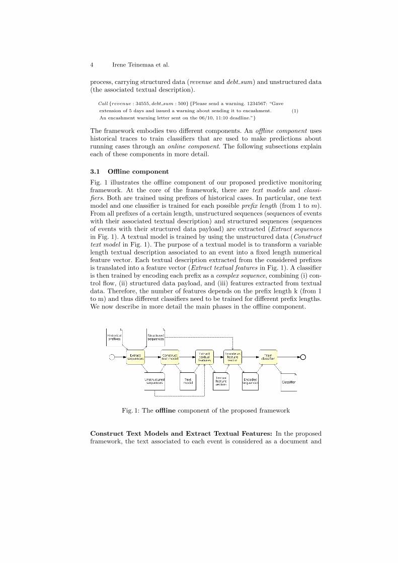
Fig. 1 illustrates the offline component of our proposed predictive monitoringframework. At the core of the framework, there are text models and classi-fiers. Both are trained using prefixes of historical cases. In particular, one textmodel and one classifier is trained for each possible prefix length (from 1 to m).From all prefixes of a certain length, unstructured sequences (sequences of eventswith their associated textual description) and structured sequences (sequencesof events with their structured data payload) are extracted (Extract sequencesin Fig. 1). A textual model is trained by using the unstructured data (Constructtext model in Fig. 1). The purpose of a textual model is to transform a variablelength textual description associated to an event into a fixed length numericalfeature vector. Each textual description extracted from the considered prefixesis translated into a feature vector (Extract textual features in Fig. 1). A classifieris then trained by encoding each prefix as a complex sequence, combining (i) con-trol flow, (ii) structured data payload, and (iii) features extracted from textualdata. Therefore, the number of features depends on the prefix length k (from 1to m) and thus different classifiers need to be trained for different prefix lengths.We now describe in more detail the main phases in the offline component.

Fig. 1: The offline component of the proposed framework

Construct Text Models and Extract Textual Features: In the proposedframework, the text associated to each event is considered as a document and


a feature vector is extracted from it. We compare 4 different techniques forextracting feature vectors from text: BoNG model with and without NB logcount ratios, LDA topic modeling, and PV.

Before feature extraction, some preprocessing is done on the unstructureddata. We start with tokenizing the documents, using simple white space tok-enization. In the case of the running example (1), the tokenization produces avector of tokens, e.g., “Please”, “send”, “a”, “warning”, . . .. Moreover, we gen-erate equivalence classes for different types of numerals by replacing them witha corresponding tag (phone number, date, or other). For example, in (1), to-ken “1234567” would be replaced by token “phone number”, token “06/10” by“date” and token “11:10” by “time”. Lastly, we lemmatize the text, i.e., we grouptogether different inflected forms of a word and we refer to such a group with itsbase form or lemma. For example, in our running example, tokens “send”, “sent”and “sending” will be clustered together into a “send” cluster (where “send” isthe lemma), whereas “deadlin” is the base form of “deadline” and “deadlines”.

In the following paragraphs, we illustrate in detail the techniques for extract-ing feature vectors from text we use in this paper.

Bag-of-n-grams (n, idf): This method is based on the BoNG model and takesas inputs two parameters: n, which is the maximum size of the n-grams; andidf , that is a boolean variable specifying whether the BoNG model is normalizedwith idf. In this method, the documents from historical prefixes are used to builda vocabulary of n-grams, V (n). Given a vocabulary V (n) of size |V (n)| = v, a

document j is represented as a vector d(j) = (g(j)t1 , g

(j)t2 , ..., g

(j)tv ), where:

g(j)ti =

{tfidf(ti

(j)) if idf

f(j)ti

otherwise

f(j)ti represents the frequency of n-gram ti in document d(j), i.e., f

(j)ti = tf(ti

(j)).For instance, in our running example (1), if n = 1, idf = false and the vocab-

ulary is V (1) = {about, agenc, collect, commun, date, deadlin, encash, extens,gave, issu, letter, number, phonenumb, pleas, send, time,warn,warning}, the vec-tor encoding the textual description would be:

d(j̄)

=(1, 0, 0, 0, 0, 1, 1, 1, 1, 1, 1, 1, 1, 1, 3, 1, 1, 3) (2)

where the word “send” (and its variations) occur three times in the document,the word “about” occurs once and the word “agency” does not occur.

Naive Bayes log count ratios (n, α): In this method, features are still basedon the BoNG model, but they are weighted with NB log count ratios, d(j) =

(f(j)t1 · r1, f

(j)t2 · r2, ..., f

(j)tv · rv). The parameter α is a smoothing parameter for

the weights [20], while n is, as in BoNG, the maximum size of the n-grams. Forinstance, if the vocabulary (and hence the term frequency) is the same as theone in (2) and the NB log count ratios vector is r = (0.85, 1.02, 0.76, 0.76, 1.52,

2.03, 1.19, 1.02, 0.45, 0.89, 1.02, 1.4, 1.39, 0.41, 1.02, 1.38, 1.27, 1.83), d(j̄) would be:

d(j̄)

= (0.85, 0, 0, 0, 1.52, 2.03, 1.19, 1.02, 0.45, 0.89, 1.02, 1.4, 1.39, 0.41, 3.06, 1.38, 1.27, 5.49) (3)


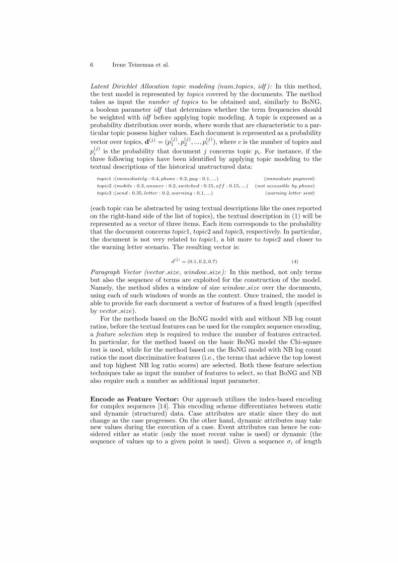
Latent Dirichlet Allocation topic modeling (num topics, idf): In this method,the text model is represented by topics covered by the documents. The methodtakes as input the number of topics to be obtained and, similarly to BoNG,a boolean parameter idf that determines whether the term frequencies shouldbe weighted with idf before applying topic modeling. A topic is expressed as aprobability distribution over words, where words that are characteristic to a par-ticular topic possess higher values. Each document is represented as a probability

vector over topics, d(j) = (p(j)1 , p

(j)2 , ..., p

(j)c ), where c is the number of topics and

p(j)i is the probability that document j concerns topic pi. For instance, if the

three following topics have been identified by applying topic modeling to thetextual descriptions of the historical unstructured data:

topic1 :(immediately : 0.4, phone : 0.2, pay : 0.1, ...) (immediate payment)

topic2 :(mobile : 0.3, answer : 0.2, switched : 0.15, off : 0.15, ...) (not accessible by phone)

topic3 :(send : 0.35, letter : 0.2, warning : 0.1, ...) (warning letter sent)

(each topic can be abstracted by using textual descriptions like the ones reportedon the right-hand side of the list of topics), the textual description in (1) will berepresented as a vector of three items. Each item corresponds to the probabilitythat the document concerns topic1, topic2 and topic3, respectively. In particular,the document is not very related to topic1, a bit more to topic2 and closer tothe warning letter scenario. The resulting vector is:

d(j̄)

= (0.1, 0.2, 0.7) (4)

Paragraph Vector (vector size, window size): In this method, not only termsbut also the sequence of terms are exploited for the construction of the model.Namely, the method slides a window of size window size over the documents,using each of such windows of words as the context. Once trained, the model isable to provide for each document a vector of features of a fixed length (specifiedby vector size).

For the methods based on the BoNG model with and without NB log countratios, before the textual features can be used for the complex sequence encoding,a feature selection step is required to reduce the number of features extracted.In particular, for the method based on the basic BoNG model the Chi-squaretest is used, while for the method based on the BoNG model with NB log countratios the most discriminative features (i.e., the terms that achieve the top lowestand top highest NB log ratio scores) are selected. Both these feature selectiontechniques take as input the number of features to select, so that BoNG and NBalso require such a number as additional input parameter.

Encode as Feature Vector: Our approach utilizes the index-based encodingfor complex sequences [14]. This encoding scheme differentiates between staticand dynamic (structured) data. Case attributes are static since they do notchange as the case progresses. On the other hand, dynamic attributes may takenew values during the execution of a case. Event attributes can hence be con-sidered either as static (only the most recent value is used) or dynamic (thesequence of values up to a given point is used). Given a sequence σi of length


k, with u static features s1i , ..., s

ui , and r dynamic features h1

i , ..., hri , the index-

based feature vector gi of σi is:

gi = (s1i , ..., s

ui , eventi1, ..., eventik, h

1i1, ..., h

1ik, ..., h

ri1, ..., h

rik).

We enhance the index-based encoding with textual features by concatenat-ing them to the feature vector. Textual data can be of both static and dynamicnature. When text contains static information, the derived v features t1i , ..., t

vi

are added to the feature vector of σi as follows:

gi = (s1i , ..., s


1i1, ..., h

1ik, ..., h

ri1, ..., h

rik, t

1i , ..., t

vi ).

On the other hand, if textual data changes throughout the case, it should behandled in the same way as dynamic structured data:

gi = (s1i , ..., s


1i1, ..., h

1ik, ..., h

ri1, ..., h

rik, t

1i1, ..., t

1ik, ..., t

vi1, ..., t

vik).

For instance, if the case containing the event in the example (1) does notcontain any static structured and unstructured data, using the topic model vec-tor in (4), the complex sequence would be:

gi

= (..., call, ..., 34555, 500, ..., 0.1, 0.2, 0.7, ...) (5)

Train Classifier: We use random forest [2] and logistic regression [10] to buildthe classifiers. Random forest has been shown to be a solid classifier in variousproblem settings, including credit scoring applications [15]. On the other hand,logistic regression, one among the most popular linear classifiers in text classifi-cation tasks, suites well to cases in which data are very sparse (this is the casewhen the BoNG model is used).

3.2 Online component

The structure of the online component of our predictive monitoring framework ispresented in Figure 2. When predicting the outcome for a running case of prefixlength k, the pre-built textual model and classifier for length k are retrieved andapplied to the running case at hand. If the prefix length of the running case islarger than the maximum prefix length m used in the training process, only thefirst m events of the running case are used.

Fig. 2: The online component of the proposed framework

Threshold minConf is an input parameter of the framework. If the classifierreturns a probability higher than minConf for the positive class, the frameworkoutputs a positive prediction. If the probability is lower than the threshold, no


prediction is made and the framework continues to monitor the case. When theobserved event is a terminal event, the final prediction is negative.

This setting, where the framework focuses only on making positive predic-tions, follows closely most real-life scenarios. Indeed, it is important for thestakeholders to filter the cases that may become deviant in the future, so thatpreventive actions can be taken. On the other hand, in cases that will likely havea normal outcome, no specific action is taken and they are allowed to continuein their own path. Still, our framework is easily extensible to early prediction ofboth positive and negative outcomes.

4 Evaluation

We have implemented the proposed methods in Python4 and evaluated their per-formance on two datasets using an existing technique for predictive process mon-itoring with structured data as a baseline [14]. Below we describe the datasets,evaluation method and findings.

4.1 Datasets

We evaluated our framework on two real-life datasets pertaining to: (i) the debtrecovery (DR) process of an Estonian company that provides credit managementservice for its customers (creditors), and (ii) the lead-to-contract (LtC) processof a due diligence service provider in Estonia.

The debt recovery process starts when the creditor transfers a delinquent debtto the company. This means that the debtor has already defaulted — failed to re-pay the debt to the creditor in due time. Usually, the collection specialist makesa phone call to the debtor. If the phone is not answered, an inquiry/reminderletter is sent. If the phone is answered, the debtor may provide an expected pay-ment date, in which case no additional action is taken during the present week.Alternatively, the specialist and the debtor can agree on a payment schedulethat outlines the repayments over a longer time period. If the collection special-ist considers the case to be irreparable, she makes a suggestion to the creditorabout forwarding the debt to an outside debt collection agency (send to encash-ment) or about sending a warning letter to the debtor on the same matter. Thefinal decision about issuing an encashment warning to the debtor and/or send-ing the debt to encashment is made by the creditor. If there is no advancementin collecting the debt after 7 days (e.g., the payment was not received on theprovided date or the debtor has neither answered the phone nor the reminderletter), the procedure is repeated.

It is in the interest of the creditor to discover, as early as possible, casesthat will not lead to any payment in a reasonable timeframe. The earlier thedebt is recovered, the more value it entails for the creditor. Moreover, suchcases are likely irreparable and could be sent to encashment without furtherdelay. Therefore, our prediction goal is to determine cases where no payment isreceived within 8 weeks after the beginning of the debt recovery process.

4 Scripts available at https://github.com/irhete/PredictiveMonitoringWithText


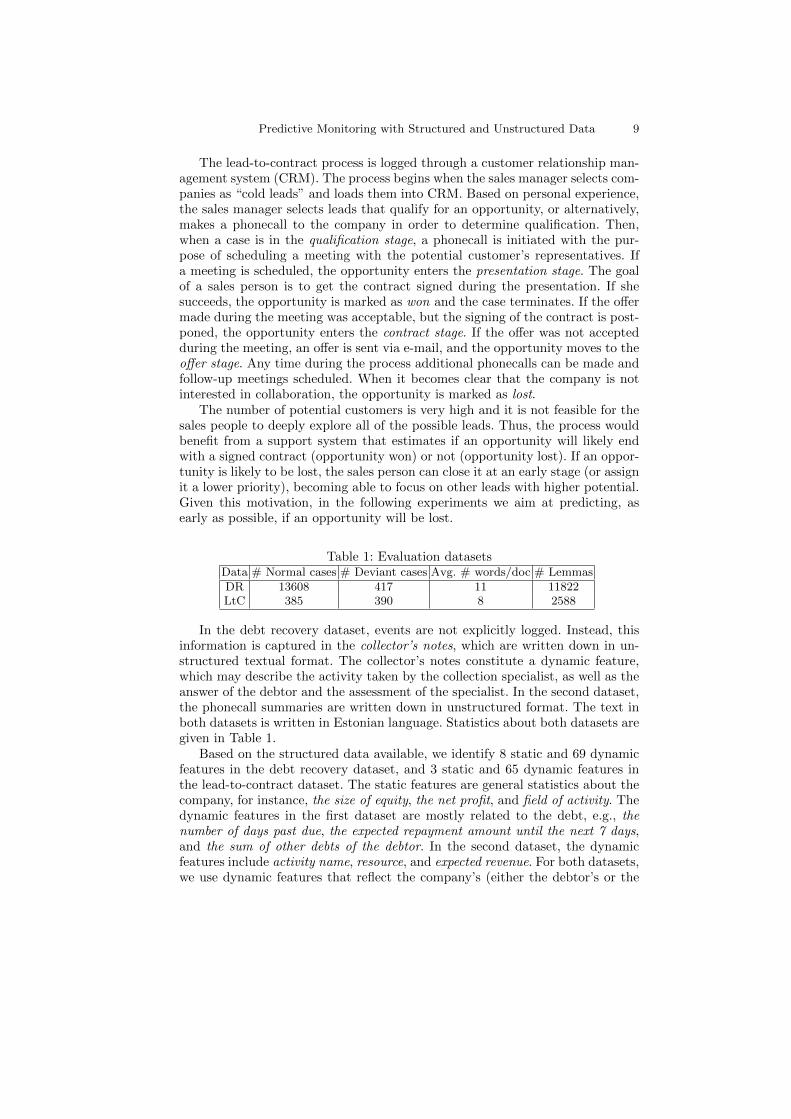
The lead-to-contract process is logged through a customer relationship man-agement system (CRM). The process begins when the sales manager selects com-panies as “cold leads” and loads them into CRM. Based on personal experience,the sales manager selects leads that qualify for an opportunity, or alternatively,makes a phonecall to the company in order to determine qualification. Then,when a case is in the qualification stage, a phonecall is initiated with the pur-pose of scheduling a meeting with the potential customer’s representatives. Ifa meeting is scheduled, the opportunity enters the presentation stage. The goalof a sales person is to get the contract signed during the presentation. If shesucceeds, the opportunity is marked as won and the case terminates. If the offermade during the meeting was acceptable, but the signing of the contract is post-poned, the opportunity enters the contract stage. If the offer was not acceptedduring the meeting, an offer is sent via e-mail, and the opportunity moves to theoffer stage. Any time during the process additional phonecalls can be made andfollow-up meetings scheduled. When it becomes clear that the company is notinterested in collaboration, the opportunity is marked as lost.

The number of potential customers is very high and it is not feasible for thesales people to deeply explore all of the possible leads. Thus, the process wouldbenefit from a support system that estimates if an opportunity will likely endwith a signed contract (opportunity won) or not (opportunity lost). If an oppor-tunity is likely to be lost, the sales person can close it at an early stage (or assignit a lower priority), becoming able to focus on other leads with higher potential.Given this motivation, in the following experiments we aim at predicting, asearly as possible, if an opportunity will be lost.

Table 1: Evaluation datasetsData # Normal cases # Deviant cases Avg. # words/doc # LemmasDR 13608 417 11 11822LtC 385 390 8 2588

In the debt recovery dataset, events are not explicitly logged. Instead, thisinformation is captured in the collector’s notes, which are written down in un-structured textual format. The collector’s notes constitute a dynamic feature,which may describe the activity taken by the collection specialist, as well as theanswer of the debtor and the assessment of the specialist. In the second dataset,the phonecall summaries are written down in unstructured format. The text inboth datasets is written in Estonian language. Statistics about both datasets aregiven in Table 1.

Based on the structured data available, we identify 8 static and 69 dynamicfeatures in the debt recovery dataset, and 3 static and 65 dynamic features inthe lead-to-contract dataset. The static features are general statistics about thecompany, for instance, the size of equity, the net profit, and field of activity. Thedynamic features in the first dataset are mostly related to the debt, e.g., thenumber of days past due, the expected repayment amount until the next 7 days,and the sum of other debts of the debtor. In the second dataset, the dynamicfeatures include activity name, resource, and expected revenue. For both datasets,we use dynamic features that reflect the company’s (either the debtor’s or the


potential customer’s) risk score, calculated at 6 different months prior to thegiven event. Moreover, as the first dataset contains a considerable amount ofmissing values, additional 16 (static) features are added that express whetherthe value of a particular feature is present or missing. In the given datasets, wedecide to use unstructured data as static information, i.e., to encode only thelast available text, given a specific prefix length.

4.2 Research Questions and Evaluation Measures

In our evaluation, we address the following three research questions:

RQ1 Do the features derived from textual data (using different methods) in-crease the prediction accuracy of index-based sequence encoding?

RQ2 Do the features derived from textual data (using different methods) in-crease the prediction earliness of index-based sequence encoding?

RQ3 Is the proposed predictive monitoring framework efficient?

For evaluating prediction accuracy (RQ1) of our framework, we use precision,recall, and F-score, as suggested in [17]. We do not use accuracy, as it can lead tomisleading results in case of imbalanced data [19]. Also, we do not report aboutspecificity, as our main goal is to predict the positive class as accurately as pos-sible. All metrics are based on the possible combinations of actual and predictedoutcomes. True positives (TP) are positive cases, which are correctly predicted aspositive. True negatives (TN) are negative cases, which are correctly predicted asnegative. False positives (FP) are negative cases, which are incorrectly predictedas positives. False negatives (FN) are positive cases, which are incorrectly pre-dicted as negatives. Given these notions, precision is defined as TP/(TP +FP ),recall as TP/(TP+FN), and F-score as 2·precision·recall/(precision+recall).

To answer RQ2, we measure the earliness of predictions [7]. Earliness iscalculated for cases that are predicted as positive, as the ratio of length of thecase when the final prediction was made / total length of the case. For instance,if the case was predicted as positive after 2 events, while the actual total lengthof the case was 8 events, earliness = 0.25. Low earliness values are better, asthe aim of predictive monitoring is to provide predictions as early as possible.

Finally, the computation time is measured in order to estimate the efficiencyof the framework (RQ3). For evaluating the offline component of the framework,we differentiate between the time for data processing (text model construction,textual feature extraction, and sequence encoding) and classifier training. Timesare summed up over all prefix lengths, in order to evaluate the total time thatis needed to set up the framework. For evaluating the online component, wecombine the time for encoding the running case as a feature vector and the timefor prediction. Times are averaged over the total number of processed events.

4.3 Evaluation Procedure

We split each dataset randomly in two parts, so that 4/5 of it is used for train-ing the offline component, while the remaining 1/5 is used for testing the on-line component. For tuning the parameters of the text modeling methods, we


perform a grid-search over all combinations of selected parameter values using5-fold cross-validation on the training set. In the DC dataset, where only 3% ofcases are deviant, we use oversampling on the training data in order to alleviatethe imbalance problem. The final Paragraph Vector models are trained for 10epochs. The optimal parameters are chosen based on F-score, for each combina-tion of text modeling method, classification method, and confidence threshold.The computation times are calculated as the average of 10 equivalent executionswith minConf = 0.6. The probability estimates returned by the classifier areused as confidence values.

The optimal parameters found when using random forest and logistic regres-sion are different. However, in the following, we discuss the values obtained usingrandom forest only, since random forest performs better than logistic regressionin all cases. We optimize the parameters described in Section 3 and use thedefault values for all the parameters not mentioned.

For the method based on the basic BoNG model, we explore 43 parametersettings (varying maximum n-gram size, idf , and number of selected features).In most cases, tf-idf weights perform slightly better than simple tf. Moreover,bigrams and trigrams gain similar performance, while both are better than uni-grams. The best number of selected features stays between 100 and 1000. In theDR dataset, only 100 features are often sufficient to gain a good accuracy, whilemore features are needed in the LtC dataset (usually 750 or 1000).

For the method based on the BoNG model with NB log count ratios, we try84 combinations of parameters (varying α, maximum n-gram size and numberof selected features). Changing the α value has almost no effect on the results,usually a small value (either 0.01 or 0.1) is chosen. The best number of selectedfeatures tends to be higher than in the BoNG case, usually between 250 and1000 features in the DR dataset and between 1000 and 5000 in the LtC dataset.In most cases, trigrams outperform bi- and unigrams.

In case of LDA (we vary the number of topics and idf), we try 6 differentnumbers of topics (12 combinations in total). In general, the larger the confi-dence, the higher the number of topics that achieves the best results. In the DRdataset, idf normalization does not improve the outcome, while changing theparameters has very little effect on the results in the LtC dataset.

For PV, we explore 91 combinations, varying the size of the feature vector andthe window size. The best results are obtained with a small 10- or 25-dimensionalvector. The optimal window size varies a lot across the experiments, but staysbetween 5 and 9, in general.

Experiments were run in Python 3.5 using scikit-learn (BoNG and classifiers),gensim (LDA and PV) and estnltk (lemmatization) libraries on a single core ofa 64-bit 2.3 Ghz AMD Opteron Processor 6376 with 378GB of RAM.

4.4 Results

The F-scores of the random forest classifiers are shown in Figures 3a (debtrecovery dataset) and 3c (lead-to-contract dataset). We observe that in bothdatasets, the methods that utilize unstructured data almost always outperformthe baseline. In the DR dataset, BoNG and NB achieve considerably better


(a) F-score in DR dataset (b) Earliness in DR dataset

(c) F-score in LtC dataset (d) Earliness in LtC dataset

Fig. 3: Predictive monitoring results with random forest

results than the other methods, while in the LtC dataset, the best results areproduced by LDA. Although the proportion of unstructured vs. structured datain the LtC dataset is much smaller than in the DR dataset, the improvementof the results is still substantial. The highest F-score in the DR dataset (0.791)is achieved by NB with minConf = 0.55, while LDA achieves F-score of 0.753with minConf = 0.65 in the LtC dataset.

Figures 3b and 3d show the prediction earliness achieved with random forest.The model with the best F-score in the DR dataset tends to make predictionswhen 59% of a case has finished, while the best model in the LtC dataset ispredicted after 40% of a case has been seen.

In order to further explore the importance of unstructured data in makingpredictions, we performed additional experiments using unstructured data only.In the DR dataset, the NB model achieves F-score of 0.66 (instead of 0.791 asin Figure 3a), while in the LtC dataset, the LDA model reaches F-score of 0.70(instead of 0.75 as in Figure 3c). In both datasets, the model trained with onlystructured data (the baseline) outperforms all unstructured data models in termsof precision, while falls behind in terms of recall. Thus, unstructured featureshave some predictive power on their own, but in order to get the most out of


the data, they should be combined with structured data. In addition, we observethat using the best model (NB, conf=0.55) of the DR dataset, 3 out of the top 5features ranked according to Gini impurity are derived from textual data. On theother hand, in the LtC dataset (LDA, conf=0.65), the first 9 features accordingto importance are structured features. This implies that in best model of theLtC dataset, textual features are less relevant than structured features.

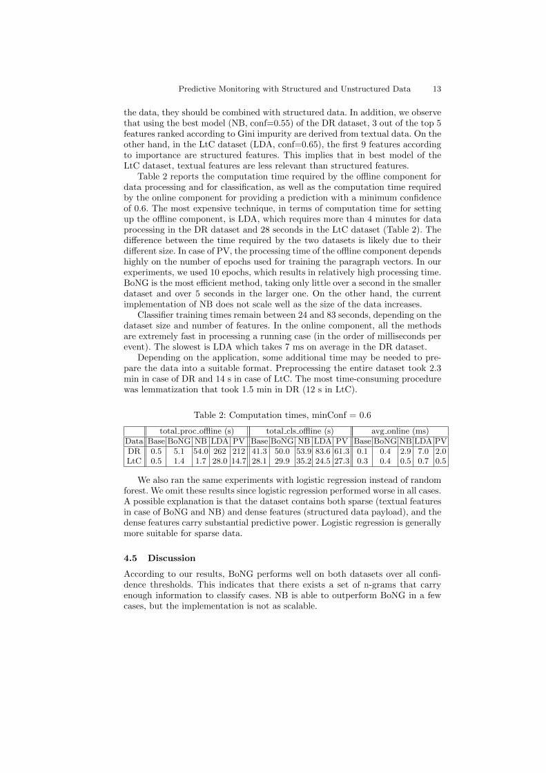
Table 2 reports the computation time required by the offline component fordata processing and for classification, as well as the computation time requiredby the online component for providing a prediction with a minimum confidenceof 0.6. The most expensive technique, in terms of computation time for settingup the offline component, is LDA, which requires more than 4 minutes for dataprocessing in the DR dataset and 28 seconds in the LtC dataset (Table 2). Thedifference between the time required by the two datasets is likely due to theirdifferent size. In case of PV, the processing time of the offline component dependshighly on the number of epochs used for training the paragraph vectors. In ourexperiments, we used 10 epochs, which results in relatively high processing time.BoNG is the most efficient method, taking only little over a second in the smallerdataset and over 5 seconds in the larger one. On the other hand, the currentimplementation of NB does not scale well as the size of the data increases.

Classifier training times remain between 24 and 83 seconds, depending on thedataset size and number of features. In the online component, all the methodsare extremely fast in processing a running case (in the order of milliseconds perevent). The slowest is LDA which takes 7 ms on average in the DR dataset.

Depending on the application, some additional time may be needed to pre-pare the data into a suitable format. Preprocessing the entire dataset took 2.3min in case of DR and 14 s in case of LtC. The most time-consuming procedurewas lemmatization that took 1.5 min in DR (12 s in LtC).

Table 2: Computation times, minConf = 0.6

total proc offline (s) total cls offline (s) avg online (ms)Data Base BoNG NB LDA PV Base BoNG NB LDA PV Base BoNG NB LDA PVDR 0.5 5.1 54.0 262 212 41.3 50.0 53.9 83.6 61.3 0.1 0.4 2.9 7.0 2.0LtC 0.5 1.4 1.7 28.0 14.7 28.1 29.9 35.2 24.5 27.3 0.3 0.4 0.5 0.7 0.5

We also ran the same experiments with logistic regression instead of randomforest. We omit these results since logistic regression performed worse in all cases.A possible explanation is that the dataset contains both sparse (textual featuresin case of BoNG and NB) and dense features (structured data payload), and thedense features carry substantial predictive power. Logistic regression is generallymore suitable for sparse data.

4.5 Discussion

According to our results, BoNG performs well on both datasets over all confi-dence thresholds. This indicates that there exists a set of n-grams that carryenough information to classify cases. NB is able to outperform BoNG in a fewcases, but the implementation is not as scalable.


In the LtC dataset, the best results are produced by LDA. The reason forthis might be that LDA combines the information captured in textual data intotopics, instead of using specific words. Thus, it is able to perform well even inthe case of few available textual data, which is the case in the LtC dataset.Also, supported by previous studies where topic modeling methods have shownto perform well on short texts, such as tweets [11], LDA is less affected by thefact that individual notes in the LtC data set contain only 8 words on average.

A possible reason for PV performing worse than the other methods is thatPV computes the feature vector for an unseen document via inference. Therefore,in order to produce reliable results, it requires a fairly large document collectionfor training. Moreover, the benefits of PV become more evident in heterogenousdatasets, where a variety of words is used to express similar concepts.

One limitation of our evaluation is its low generalizability. While the eval-uation datasets come from two real-life processes with different deviant caseratios (balanced vs. imbalanced), the textual notes in both datasets are writtenby members of a small team of debt recovery specialists and salespeople respec-tively. The observations might be different if these notes were written by a largerteam or if they included emails sent by customers (higher heterogeneity). Also,the results may be affected by the amount of textual data available. Anotherlimitation is the reduced set of classification algorithms employed (random for-est and logistic regression). While these algorithms are representative and widelyused in text mining, other classifiers might be equally or more suitable.

5 Related Work

Predictive monitoring is relevant in a range of domains where actors are in-terested in understanding the future performance of a system in order to takepreventive measures. Predictive monitoring applications can be found in a widerange of settings, including for example industrial processes [12] and medicaldiagnosis [4]. One recurrent task addressed in this field is that of failure predic-tion [19] – i.e., detecting that a given type of failure will occur in the near-term.

While the predictive monitoring problems addressed in the above fields sharecommon traits with the problem addressed in this paper, business process eventlogs have a specific characteristics that call for specialized predictive monitoringmethods, chiefly: (i) business process event logs are structured into cases andeach case can have a different outcome; hence, the problem is that of monitoringmultiple concurrent streams of events rather than one; (ii) every event in a caserefers to a given activity or external stimulus; (iii) every event has a payload;(iv) the payload may contain both structured data and text, and the structuredpart of the data includes both discrete and numerical attributes. In contrast,in other application domains [12, 19, 4], events in a given stream are generallyof homogeneous types and carry numerical attributes (e.g., measurements takenby a device), this requiring a different type of techniques compared to predictivebusiness process monitoring.

A range of methods have been proposed in the literature to deal with thisspecific combination of characteristics. These methods differ in terms of the


object of prediction, the type of data employed, and the approach used for featureencoding. With respect to the former, some approaches focus on predicting timeor other performance measures. For example, [18] uses stochastic Petri nets topredict the remaining execution time of a case, while [17] addresses the problemof predicting process performance violations in general and deadline violations inparticular. Other approaches focus on predicting the outcome of a process, suchas predicting failures or other types of negative outcomes (a.k.a. deviance). Forexample, [6] presents a technique to predict risks, while [16] focuses on predictingbinary outcomes (normal vs. deviant cases).

Predictive process monitoring approaches also differ depending on the typeof data they use. Some approaches only use control-flow data [18, 17], others usecontrol-flow and structured data [9, 16, 6, 14]. When building predictive processmonitoring models that take into account both control-flow and data payloads,a key issue is how to encode a given trace in the log (or a prefix thereof) asa feature vector. In this respect, a comparison feature encoding approaches isgiven in [14], which empirically shows that an index-based encoding approachprovides higher performance.

None of the above studies have taken into account textual data. Yet, textualdata is generated in a range of customer-facing processes and as shown in thispaper, can enhance the performance of predictive process monitoring models.

6 Conclusion

We outlined a framework for predictive process monitoring that combines textmining methods to extract features from textual documents, with (early) se-quence classification techniques designed for structured data. We studied dif-ferent combinations of text mining and classification techniques and evaluatedthem on two datasets pertaining to a debt recovery process and a sales process.

In the reported evaluation, BoNG and NB, in combination with random for-est, outperform other techniques when the amount of textual data is sufficientlylarge. In the presence of a smaller document collection, LDA exhibits betterperformance. An avenue for future work is to further validate these observationson other datasets exhibiting different characteristics, for example, datasets con-taining longer or more heterogeneous documents. Another future work avenue isto produce interpretable explanations of the predictions made, so that processworkers and analysts can understand the reasons why a given case is likely toend up with a given outcome. Last but not least, we are planning to integrateour tool in the operational support of the process mining tool ProM to providepredictions starting from an online stream of events.

Acknowledgments This research is funded by the EU FP7 Programme (projectSO-PC-Pro) and by the Estonian Research Council and by ERDF via the Soft-ware Technology and Applications Competence Centre (STACC).

References

1. Blei, D.M., Ng, A.Y., Jordan, M.I.: Latent dirichlet allocation. the Journal ofmachine Learning research 3, 993–1022 (2003)


2. Breiman, L.: Random forests. Machine learning 45(1), 5–32 (2001)3. Castellanos, M., Casati, F., Dayal, U., Shan, M.: A comprehensive and automated

approach to intelligent business processes execution analysis. Distributed and Par-allel Databases 16(3), 239–273 (2004)

4. Clifton, L.A., Clifton, D.A., Pimentel, M.A.F., Watkinson, P., Tarassenko, L.: Pre-dictive monitoring of mobile patients by combining clinical observations with datafrom wearable sensors. IEEE J. Biomedical and Health Informatics 18(3), 722–730(2014)

5. Conforti, R., de Leoni, M., Rosa, M.L., van der Aalst, W.M.P., ter Hofstede,A.H.M.: A recommendation system for predicting risks across multiple businessprocess instances. Decision Support Systems 69, 1–19 (2015)

6. Conforti, R., de Leoni, M., Rosa, M.L., van der Aalst, W.M.P., ter Hofstede,A.H.M.: A recommendation system for predicting risks across multiple businessprocess instances. Decision Support Systems 69, 1–19 (2015)

7. Di Francescomarino, C., Dumas, M., Maggi, F.M., Teinemaa, I.: Clustering-BasedPredictive Process Monitoring. arXiv preprint (2015)

8. Dumas, M., La Rosa, M., Mendling, J., Reijers, H.A.: Fundamentals of BusinessProcess Management. Springer (2013)

9. Folino, F., Guarascio, M., Pontieri, L.: Discovering context-aware models for pre-dicting business process performances. In: OTM, pp. 287–304. Springer (2012)

10. Freedman, D.: Statistical Models: Theory and Practice. Cambridge UniversityPress (Aug 2005)

11. Hong, L., Davison, B.D.: Empirical study of topic modeling in twitter. In: Pro-ceedings of the first workshop on social media analytics. pp. 80–88. ACM (2010)

12. Juriceka, B.C., Seborga, D.E., Larimore, W.E.: Predictive monitoring for abnormalsituation management. Journal of Process Control 11(2), 111–128 (2001)

13. Le, Q.V., Mikolov, T.: Distributed representations of sentences and documents.arXiv preprint arXiv:1405.4053 (2014)

14. Leontjeva, A., Conforti, R., Di Francescomarino, C., Dumas, M., Maggi, F.M.:Complex symbolic sequence encodings for predictive monitoring of business pro-cesses. In: BPM, pp. 297–313. Springer (2015)

15. Lessmann, S., Baesens, B., Seow, H.V., Thomas, L.C.: Benchmarking state-of-the-art classification algorithms for credit scoring: An update of research. EuropeanJournal of Operational Research 247(1), 124–136 (2015)

16. Maggi, F.M., Di Francescomarino, C., Dumas, M., Ghidini, C.: Predictive moni-toring of business processes. In: CAiSE 2014. pp. 457–472 (2014)

17. Metzger, A., Leitner, P., Ivanovic, D., Schmieders, E., Franklin, R., Carro, M.,Dustdar, S., Pohl, K.: Comparing and combining predictive business process mon-itoring techniques. IEEE Transactions on SMC 45(2), 276–290 (2015)

18. Rogge-Solti, A., Weske, M.: Prediction of remaining service execution time usingstochastic petri nets with arbitrary firing delays. In: ICSOC. pp. 389–403 (2013)

19. Salfner, F., Lenk, M., Malek, M.: A survey of online failure prediction methods.ACM Computing Surveys (CSUR) 42(3), 10 (2010)

20. Wang, S., Manning, C.D.: Baselines and bigrams: Simple, good sentiment and topicclassification. In: Annual Meeting of the Association for Computational Linguistics.pp. 90–94 (2012)

predictive business process monitoring with structured and

Documents