prediction of turbine rotor blade forcing due to in

1 Copyright © 2011 by ASME

PREDICTION OF TURBINE ROTOR BLADE FORCING DUE TO IN-SERVICE STATOR VANE TRAILING EDGE DAMAGE

Marcus Meyer, Roland Parchem, Peter Davison Rolls-Royce Deutschland Eschenweg 11, Dahlewitz

D-15827 Blankenfelde-Mahlow Germany

ABSTRACT In the following paper we will present an overview on the

results of a research project whose objective is the assessment

of the influence of trailing edge material loss of high pressure

turbine nozzle guide vanes onto the low engine order excitation

of the downstream rotor blade. To quantify the forcing, the

modal forces for the rotor eigenmodes of interest are obtained

by solving the unsteady Navier-Stokes equations for a full

assembly of stator and rotor ring. Since the computing

resources for such a calculation are too high to be routinely

employed for the assessment of in-service damage patterns, an

important task of the project was to investigate quick

alternatives to the costly CFD simulations. The approach

chosen is to perform a sufficient number of forced response

calculations with different damage patterns in advance and use

the results to build a surrogate model that can be used to assess

the severity of damage patterns by simple interpolation. We will

first present the analysis chain employed to quantify the

forcing, next describe the approach to build a surrogate model

with special focus on the generation of an optimal DoE matrix,

and finally discuss the prediction accuracy of the surrogate

model. It is shown that an interpolating surrogate model, based

on radial basis functions, can successfully be used to predict

the rotor forcing for damage patterns that were not analyzed

using the costly CFD calculations beforehand.

INTRODUCTION In this contribution we will give an overview on the results

of a research project dedicated to the analysis of rotor forcing

due to in-service damage. During the operation of jet engines it

is possible that at the end of the nominal component life

damage occurs at the trailing edges of the high pressure turbine

nozzle guide vanes (HPT NGVs): Due to the extremely high

temperatures in this region of the engine, which on average

exceed the melting temperature of the employed vane material

by more than 300 degrees during takeoff, any unintended

decrease of the vane cooling mass flow can lead to a loss of

trailing edge material, exemplary depicted in fig. 1. The

structure of the NGV can withstand a significant amount of

trailing edge material loss, thus the damage is posing no

imminent threat to the operation of the engine.

Fig. 1: Nozzle guide vane showing trailing edge material loss and the idealized shape parameterization

But additionally the damage changes the flow through the

affected passage, thus causing a so-called low engine order

excitation of the rotor bladerow downstream [1]. During normal

operation of the engine a small amount of low order excitation

is always present due to allowable tolerances in the static

components, but the larger throat width variation caused by

trailing edge material loss can lead –in extreme cases– to high

cycle fatigue failure of a rotor blade, caused by a resonance in

the operating range, which clearly has to be avoided at all cost.

These resonances can be visualized in the so-called Campbell

diagram, exemplary depicted in fig. 2 for an HPT rotor: In this

Proceedings of ASME Turbo Expo 2011 GT2011

June 6-10, 2011, Vancouver, British Columbia, Canada

GT2011-45204

1 Copyright © 2011 by Rolls-Royce Deutschland Ltd. & Co. AG


example low engine orders (EO) in the interval from 7 to 12

intersect the frequency of the first rotor eigenmode in the

operating range of the engine.

Fig. 2: Campbell diagram showing resonances for main and low engine order excitation

Thus it is very important to be able to accurately quantify the

damage-induced rotor forcing if trailing edge damage is

detected during routine engine inspections. Based on the shape

(and circumferential distribution of the damage if more than one

damaged vane is present), a maintenance schedule of the engine

in question has to be assigned, which maximizes on-wing time

without compromising the safe operation of the engine.

Unfortunately both the individual shape of the damage as well

as the circumferential distribution will be different from case to

case. In addition it is necessary to solve the unsteady flow for a

full NGV and rotor ring, typically modeled using the unsteady

Reynolds-averaged Navier-Stokes equations (URANS) in order

to accurately quantify the rotor forcing. Due to the large mesh

that is required (approximately 40 million grid points) and the

low frequency content that needs to be resolved, such a flow

calculation can require up to 10 days on 40 cores on a high-

performance cluster. This is clearly too time- and CPU-resource

consuming for routine use. On the other hand a growing fleet of

engines that enter service necessitate the capability of quick

assessment of in-service damage patterns, defined by individual

damage shapes and their circumferential distribution. Thus an

important task of the research project at hand is to find an

accurate prediction method with quick turnaround times. Our

presentation is consequently structured into two parts: First we

will describe the setup of the CFD simulation required for the

quantification of rotor forcing and present steady and unsteady

CFD results for a representative trailing edge damage. In the

second part we will present the approach to build a surrogate

model, investigate different surrogate formulations and assess

the accuracy of the prediction results. The paper concludes with

a summary and recommendations for future steps.

PART I - CFD ANALYSIS

The computations presented in this paper are performed

using the Rolls-Royce proprietary code AU3D, an unsteady

flow and aeroelasticity solver [2,3], which is based on

unstructured meshes [5], thus offering high flexibility for

modeling complex geometric shapes. The code solves the

URANS equations with Spalart-Allmaras turbulence model and

has been validated for a wide range of turbomachinery flows

[4]. The structural part of the solver employs a modal model

obtained from a 3D finite element representation of the rotor

blade. The structural mode shapes (as example the first

eigenmode of a typical HPT rotor blade is shown in fig. 3) are

interpolated onto the fluid mesh in a preprocessing step. During

the unsteady computation the structural and fluid boundary

conditions, i.e. displacements and pressures, are exchanged at

every time step. Although the solver permits movement of the

fluid mesh to represent the instantaneous shape and position of

the structure undergoing deformation under the influence of the

fluid forces, the forced response calculations described in this

paper are performed without mesh motion.

Fig. 3: First eigenmode of a typical HPT rotor blade

This decoupled approach, which is commonly employed

for HPT rotor blades, reduces computing time and allows the

computation of the forces acting on several eigenmodes and

nodal diameters at once. (The nodal diameter denotes the

number of vibration cycles around the circumference of the

rotor ring.) This is important in our case because we do not

know in advance which nodal diameter and eigenmode is

excited the most by the damaged assembly under consideration.

The modal forces obtained from the CFD solution are used in a

subsequent step to calculate the rotor blade displacements and

stresses, taking into account nonlinear elements such as under-

platform dampers or seal wires, if present, using a frequency-

domain nonlinear solver, see [12] and the references therein.



Grid generation

The assembly studied in this paper is representative of the

first stage of modern high-pressure turbines. The geometry is

taken from [13], where additional details on design and airfoil

shapes can be found. Although the first two bladerows of high

pressure turbines are normally cooled, the cooling flows were

omitted in this study to allow comparison with the results of an

upcoming measurement campaign, where cooling flows are also

not present. The grids used for NGV and rotor blade row are

hybrid meshes, consisting of 10 hexahedral element layers in

the boundary layer and prismatic elements in the rest of the

passage, see fig. 4. The meshes are unstructured in the blade-to-

blade plane and the 3D grid is obtained by sweeping the

unstructured mesh along the blade span [5]. The radial

distribution of 100 grid layers and the parameterization of the

unstructured mesh follows the recommendations of a mesh

refinement study [7], undertaken to find reasonably sized

meshes of high accuracy for this application. The resulting grid

sizes of a single NGV and rotor blade passage are 400k points

and 235k points, respectively, leading to a grid size of 32

million points for the full 2-row assembly, as shown in fig. 5

right.

Fig. 4: Meshes used for datum vane (top), vane with triangular damage (middle) and rotor (bottom)

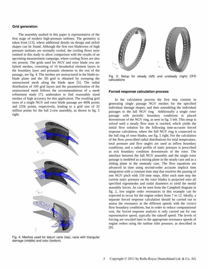
Fig. 5: Setup for steady (left) and unsteady (right) CFD calculations

Forced response calculation process

In the calculation process the first step consists in

generating single passage NGV meshes for the specified

individual damage shapes, and then assembling the individual

passages to the full NGV ring. Additionally a single rotor

passage with periodic boundary conditions is placed

downstream of the NGV ring, as seen in fig. 5 left. This setup is

solved until a steady flow state is reached, which yields the

initial flow solution for the following time-accurate forced

response calculation, where the full NGV ring is connected to

the full ring of rotor blades, see fig. 5 right. For the calculation

of the flow, prescribed radial distributions for total temperature,

total pressure and flow angles are used as inflow boundary

conditions, and a radial profile of static pressure is prescribed

as exit boundary condition downstream of the rotor. The

interface between the full NGV assembly and the single rotor

passage is modeled as a mixing plane in the steady case and as a

sliding plane in the unsteady case. The flow equations are

advanced in time using second-order accurate implicit time

integration with a constant time step that resolves the passing of

one NGV pitch with 150 time steps. After each time step the

current static pressure on the rotor blades is projected onto all

specified eigenmodes and nodal diameters to yield the modal

assembly forces. As can be seen from the Campbell diagram in

fig. 2, low engine order resonances in this example can be

expected to occur for the engine orders from 7 to 12. Ideally, a

separate forced response calculation should be carried out to

assess the resonance at the different speeds with the correct

flow boundary conditions, but in order to reduce computational

cost, the forced response analysis is only carried out for one

representative speed, typically the takeoff speed. The levels of

forcing are rescaled later to the appropriate resonance speeds of

engine orders using the turbine inlet pressure, as described in

[8].



Steady CFD analysis of a single damaged vane

In the following section we will present the results of the

steady CFD analysis of a setup as depicted in fig. 5 (left). The

NGV ring in this case includes one vane with a triangular

damage, as shown in fig. 6. The large damage leads to the

development of two strong vortices, which is shown in fig. 7,

where the total pressure in the outlet plane of the NGV ring is

depicted. It can be seen that the damage induces a window

where the flow is turned significantly less than the flow in the

undamaged vane passages, but the strong distortion is limited to

a single passage left and right of the damaged vane. The wakes

of the neighboring passages are affected only to a very small

degree. This can also be clearly seen in fig. 8, where the Mach

number on a radial cut at vane mid height is shown. Clearly the

distortion is limited to the passages left and right of the damage.

In addition we can see that the damage induces a region with an

increased velocity on the suction side of the vane left to the

damaged vane, which also leads to a reduction of the static

pressure as seen in fig. 6. The influence of the distorted flow on

the downstream rotor blade has to be assessed by an unsteady

calculation, as presented in the next section.

Fig. 6: Single triangular damaged vane surrounded by undamaged vanes

Fig. 7: Total pressure in the NGV exit plane behind a single triangular damage

Fig. 8: Mach number on a radial cut at vane mid height

Unsteady results and low engine order excitation

In this section we will first describe the unsteady CFD

results of the setup presented above, where a single vane with

triangular damage is inserted into a ring with otherwise

undamaged vanes, see fig. 9, where for clarification some of the

rotor blades have been blanked, although the CFD setup

includes the full rings of vane and rotor, as shown in fig. 5 right.

As shown above in the analysis of the steady flow, the distortion

is limited to the passage left and right of the damaged vane. The

large window of flow with a significant under-turning compared

to the non-distorted flow changes the loading of the rotor blade,

as seen in fig. 10. Here the axial and tangential force per unit

length on a radial cut at mid height of the rotor is compared for

the undamaged case (dashed) and the passing of the damaged

vane (full line), whose location is shown in fig. 9 together with

lines indicating the corresponding time steps in fig. 10 below. It

can be seen that the rotor first experiences an unloading in the

tangential direction, followed by a stronger positive loading.

This change of loading can excite the flap modes of the rotor

blade, which we can assess by calculating the modal assembly

force during the unsteady simulation, as described next.

To assess the modal forces for the low engine order

excitation, the forced response analysis is carried out for 3500

time steps. This ensures that the modal force time history

contains four cycles of the lowest (7th) engine order of interest,

from which only the two last cycles will be used for the spectral

analysis of the frequency content. As an example we will use the

assembly depicted in fig. 11, where a large number of vanes

with different damage sizes are placed randomly over the

circumference. In fig. 12 the modal force of the 4th mode / 34th

nodal diameter (ND) is compared for an undamaged and the

randomly damaged assembly. Here mode 4/ND 34 corresponds

to the main engine order excitation of the assembly. It can be

seen that the amplitude of this excitation is lower for the

damaged assembly, thus energy is redistributed to other

frequencies, for example the mode 1/ND 7 excitation, which is



shown in fig. 13. This excitation is not present at all in the

undamaged assembly, but shows a significant modal force

content for the damaged assembly. Which nodal diameter is

excited the most depends on the frequency content of the flow

and thus on the circumferential distribution of the damaged

vanes. For the assembly depicted in fig. 12, the highest

excitation is obtained for the 8th nodal diameter, as can be seen

in fig. 14, where all low nodal diameter excitations of interest

are compared.

Fig. 9: Rotor passing a vane with triangular damage

Fig. 10: Comparison of axial and radial rotor force per unit length at mid-height (dashed: undamaged, full: damaged assembly)

Fig. 11: NGV assembly with a large number of damaged vanes at random circumferential locations

Fig. 12: Modal assembly force over time for mode 4 and nodal diameter 34 for undamaged (design 0) and randomly damaged case

Fig. 13: Modal assembly force over time for mode 1 and nodal diameter 7 for undamaged and randomly damaged case

Fig. 14: Modal assembly forces for selected low nodal diameters over time for the randomly damaged case



PART II - SURROGATE MODELLING

An important task of the project is to develop an approach

for a quick but accurate assessment method, which can deliver

an answer in the order of minutes, i.e. does not require 10 days

and an unsteady CFD analysis to quantify the rotor forcing. It

was decided to employ an approach based on surrogate

modeling techniques due to its general applicability. This

approach requires a sufficiently high number of representative

trailing edge damage shapes and their circumferential

distributions to be simulated in advance using the CFD process

described in the section above. Then a surrogate model is fitted

to the CFD results and used for future predictions. In order for a

surrogate based approach to be set up, we firstly need to define

the input variables, secondly select an efficient Design-Of-

Experiment (DoE) matrix, thirdly automate and run the process

to perform the CFD calculation as well as its postprocessing,

and finally decide on the functional form and fit the surrogate

model to the data. These steps will be described in the

following paragraphs.

Parameterization

The shape of the individual trailing edge material loss can

for example be approximated with a trapezoid, as shown

schematically in fig. 1. This parameterization requires five

values to be specified for each damage, which has to be

multiplied by the number of NGVs, typically of the order of 40,

to arrive at the final dimension of the surrogate model space, in

this case leading to a dimension of 40x5=200. This is clearly

too high taking into account that a single forced response

calculation requires 10 days on 40 cores, and at least 5 to 10

calculations should be performed per dimension. In order to

reduce the dimensionality of the problem, an investigation of

damage shapes which occur in service was carried out: Each of

the available shape examples is approximated with a trapezoid.

A subsequent statistical analysis of the resulting parameter

values shows that fortunately (a) the damages mostly occur at

midspan and (b) that the individual shape can be reconstructed

from the area of the shape alone with a high degree of

correlation. This means that if the area of the missing material is

known, the shape which is most probable for this amount of

missing area is given by an explicit functional relationship,

shape = f(area). That greatly reduces the dimensionality of the

problem to only a single free parameter per NGV. In addition it

lowers the threshold for adoption of the proposed method in

practice, since the effort to measure the size of missing trailing

edge area is small, using for example an electronic borescope

during routine in-service inspection.

The free parameters of our DoE setup are thus only the

damage areas a of the individual NGVs. In addition we assign

an upper bound to a based on experience. In order to limit the

number of meshes of damaged NGVs that have to be generated

for the DoE, a certain number of discrete levels ai are selected,

equally spaced between undamaged and maximal damage area.

In our case i=6, leading to 7 different NGVs including the

undamaged case, which form the building blocks of all

damaged assemblies.

Generation of the DoE matrix

Before we proceed to generate the actual DoE matrix, we

have to take into account the rotational symmetry of the CFD

setup: It is common practice to ignore the circumferential

variation of temperature, pressure and velocity, due to the

integer number of burner cans spaced around the circumference.

Instead a circumferentially averaged radial distribution of the

combustor exit profile is specified. Thus the CFD assembly

under consideration is rotationally symmetric with respect to the

resulting forcing levels, even when trailing edge damages are

present: Any duplicate of a damaged NGV ring that is created

by rotating the whole NGV ring by an integer multiple of the

pitch angle will yield the same forcing on the downstream rotor

ring as the original non-rotated assembly. This fact fortunately

reduces the required number of designs significantly, since each

design point in the initial DoE matrix introduces all its rotated

copies into the final "rotated" design matrix without the need to

perform individual forced response calculations of these rotated

copies. This will be exploited in the setup of the DoE matrix as

follows: The matrix is built up from three parts: The first

designs are selected to be single NGV damage cases of each

discrete level ai, since those single damage cases are believed to

occur most frequently during operation. The second set of

designs are selected to be those cases that excite a pure engine

order frequency in the engine operating range, i.e. the “worst

case” scenarios. Those pure engine order excitation cases are

created by placing 7 to 12 NGVs with maximal damage level as

equally spaced as possible on the circumference of the NGV

ring. The last set of 30 additional designs are chosen in such a

way to evenly fill the design space (space-filling design). This

can be achieved by using a simulated annealing optimization

algorithm as described in [6]: Starting from an initial Latin

hypercube design, the algorithm iteratively seeks to improve the

space filling criterion, in our case the maximization of the

minimal distance: A Latin hypercube design is called “maximin”

when the separation distance mini≠j ||xi - xj|| is maximal among

all Latin Hypercube designs of a given size. The distance is

calculated for all possible combinations of (rotated) design

sites. The algorithm selects “low-performing” designs which

exhibit minimal distance and perturbs randomly selected entries

of the corresponding design vectors to improve the space filling

criterion. The minimal distances are evaluated also for all

rotated copies of all designs in order to take the rotational

symmetry into account and the algorithm is allowed to change

only the last 30 designs in order to preserve the first two sets of

the design matrix. The optimization is repeatedly started from

different randomly generated initial Latin hypercube designs

and the best solution found after several hundred optimization

runs is selected as our final design matrix. If the rotational

symmetry is taken into account, the resulting 43 designs



represent a total of 1620 designs including the rotated copies,

i.e. approximately 40 designs per degree of freedom. This

number of points should be more than enough for the generation

of an interpolating surrogate model with sufficient accuracy, as

presented in the next section.

Surrogate model generation

Surrogate models, also called metamodels or response

surfaces, can be subdivided into approximating and

interpolating models. The approximating models are chosen

when the output to be modeled contains random errors, for

example when the results are obtained by performing

measurements in the laboratory. In our case the results are

obtained by performing computer experiments, and depend

deterministically on the input parameters: If the same input

parameters, i.e. damage areas for the NGVs in the assembly, are

used for two forced response calculations, both will exhibit the

same resulting modal force amplitudes. Thus in the case of

computer experiments an interpolating model is the better

choice [14]. For scattered data points in a high-dimensional

space, the interpolating surrogate models which are most often

employed are radial basis functions (RBF) [9], Kriging [10] and

neural networks [11]. Since in our case the number of

interpolations points (1620) and the dimension of the problem

(40) are quite high, the optimization steps in both the Kriging

and neural network approach can be very time consuming. Thus

we will start with a radial basis function model and check the

approximation quality using a cross validation technique. For

the radial basis function model, the user has to specify the kind

of basis function to use and the degree of the polynomial for the

approximation of the global trend. In our case the functional

form of the RBF model is given by

∑∑==

−+=M

j

jj

m

k

kk xxbxaxy11

)()()( ϕπ

where the first term denotes the polynomial used to approximate

the global trend and the second term the radial basis functions

which describe the deviations of the model from the global

function in order to obtain an interpolating model. The vector

x denotes our free variables, i.e. the values of the missing area

for each of the NGVs. Additional information on RBF models

can be found in [9] and the references therein.

The correct choices for kernel φ and polynomial degree m

are not obvious and differ from application to application. Thus

we take a brute-force approach and fit RBF models for all

possible combinations of basis function and polynomial degree,

evaluate the goodness of fit by performing a cross validation for

each model and finally select the model which displays the

lowest error. The cross validation is performed by sequentially

removing a single design from the full design matrix and

rebuilding the RBF model with the reduced set of design points.

Then the interpolated value for the removed design obtained

from the RBF model is compared with the actual, known value,

thus obtaining an error measure. The final root-mean-square

(RMS) value of all relative error measures is used to select the

best model for our application. The results of the cross

validation are shown in fig. 15 for the 8th

EO case and in fig.

16 for the 12th

EO case. The kernel IDs correspond to the

kernels {linear, cubic, thinplatespline, multiquadric, gaussian}

and polynomial degrees {0,1}. These kernels are given by the

functions

)(

)(

)(

)(

)(

||)exp(||

||||

||)log(||||||

||||

||||

)(22

2

3

Gaussian

icmultiquadr

plinethinplates

cubic

linear

z

z

zz

z

z

z

+

=

γ

ϕρ

where z denotes the distance |||| jxx − . Since all RBF models

with a polynomial degree 2 did exhibit a significantly higher

error, they have been omitted from the figures 15 and 16.

Fig. 15: Relative root mean square error for 8

th EO content

approximation with different radial basis function models

Fig. 16: Relative root mean square error for 12

th EO content

approximation with different radial basis function models

It can be seen that the influence of kernel and degree of

polynomial on the RMS error is not very high, all models

exhibit a relative error of around 15% for the 8th

and 11% for

the 12th

EO case, which is surprisingly low given the very small

number of only 43 CFD simulations that were performed. To



improve the accuracy of the surrogate model, additional points

can be added to the Design-of-Experiments matrix to improve

the space-filling property. Another approach would be to switch

to a Kriging surrogate model, which can be thought of as an

optimized RBF model. In the Kriging model a typical kernel is

given by the parameterized Gaussian kernel,

)||exp()(1

lp

l

d

l

l zz ∑=

−= θϕ

where the free parameters θl can be thought of as

"importance" factors, describing the influence of the individual

input variable onto the surrogate response [15]. Since in our

case, due to the rotational symmetry of the setup, it can be

argued that each input variable is equally important, the

optimization task to fit the Kriging model is simplified to a

single-variable optimization, i.e. finding the θl = θ which

minimizes the Kriging MLSE error, or a two-variable

optimization problem if also the exponent pl=p is allowed to

vary. In order to assess the potential of improvement that can be

gained by this optimization, a simple test is performed, where

the RBF model with a Gaussian kernel is fitted for different

values of theta in the range from 0.1 to 100 and the accuracy of

the individual models is again estimated using the cross-

validation approach. This test shows that the RMS error can be

reduced by selecting the optimal theta value, but only by a small

fraction of about 0.4%. Thus it can be concluded that the

“tuned” RBF model with exponent p=2 and Gaussian Kernel is

well suited for our application: In fig. 17 the model predictions

for two different exponents (p=1 and p=2) are compared with

the original data for a one-dimensional cut using the single-

damage cases as reference. It can bee seen that the tuned RBF

model with p=2 approximates the original data very well.

Fig. 17: Comparison of optimized Kriging model for exponents p=1 and p=2 with the original data (NGV ring with single damage of different size)

The resulting surrogate model can thus be used to predict the

rotor forcing for assemblies that were not in the initial “training

set”, i.e. the initial DoE matrix. The expected maximal error

due to the interpolation model can be accounted for using a

safety factor. In addition those designs that come up during

service and are “far away” from the pre-computed designs can

be analyzed with the unsteady CFD simulation. Then their

forcing values are added to the surrogate model, thus creating a

process of constant improvement of the surrogate model, based

on the feedback from in-service inspections.

CONCLUSIONS AND OUTLOOK

In this paper the low engine order excitation of a high

pressure turbine rotor blade due to NGVs with damaged trailing

edges has been analyzed with the aim to generate a surrogate

model for the quick assessment of damage severity. Due to the

very high computing resources that are required for the analysis

of low engine order excitation, the dimensionality of the design

space has to be reduced as much as possible, which has been

accomplished by a suitable parameterization of the damage

shape, based on a statistical analysis. The process to generate a

customized optimal design-of-experiment matrix that takes into

account the rotational symmetry of the problem has been

described. The generation of RBF surrogate models and its

approximation quality has been presented. Future steps will aim

at reducing this error by placing additional points at carefully

selected design sites, based on in-service feedback. Additionally

the sensitivity of modal force to the shape parameterization will

be investigated to obtain an indicator of the error and possibly

correction factors to account for the approximation of the

individual damage shape by the simplified regression-based

trapezoidal shape. Finally the results of an upcoming

measurement campaign will be used to validate the CFD results,

which will be described in a follow-up paper.

ACKNOLEDGEMENTS

The funding of this work under LUFO IV, Call I, Project

RobusTurb, contract number 20T0608A is gratefully

acknowledged. In addition the authors want to thank Dr. di

Mare, Imperial College, London, for many helpful discussions,

and Rolls-Royce Deutschland for allowing the publication of

this work.

REFERENCES

[1] Breard, C., Green, J. H., Imregun,M.: Low-engine-

order excitation mechanisms in axial-flow turbomachinery,

Journal of Propulsion and Power, Vol. 19, No. 4, pp. 704-712,

2003.

[2] Sayma, A. I., Vahdati, M., Sbardella, L., Imregun, M.:

Modeling of three-dimensional viscous compressible

turbomachinery flows using unstructured hybrid grids. AIAA

Journal, Vol. 38, No. 6, pp. 945-954, 2000



[3]Vahdati, M., Sayma, A.I., Imregun, M.: An integrated

nonlinear approach for turbomachinery forced response

prediction. Part I: Formulation. Fluids and Structures, Vol. 14,

No. 1, pp. 87-101, 2000.

[4]Vahdati, M., Sayma, A.I., Imregun, M.: An integrated

nonlinear approach for turbomachinery forced response

prediction. Part II: Case studies. Fluids and Structures, Vol. 14,

No. 1, pp. 103-125, 2000.

[5] Sbardella, L., Sayma, A.I., Imregun, M.: Semi-

structured meshes for axial turbomachinery blades.

International Journal for Numerical Methods in Fluids, Vol. 32,

No. 5, pp. 569-584, 2000

[6] Husslage, B., Rennen, G., van Dam, E., den Hertog, D.:

"Space-Filling Latin Hypercube Designs for Computer

Experiments" (March 2006). Available at SSRN:

http://ssrn.com/abstract=895464

[7] Popig, F.: Numerische Analyse der Strömung in einer

Statorpassage mit beschädigter Hinterkante. Studienarbeit,

Technische Universität Cottbus, 2008

[8] Green, J.S., Fransson, T.: Scaling of Turbine Blade

Unsteady Pressures For Rapid Forced Response Assessment,

GT2006-90613, Proceedings of the ASME TurboExpo, 2006

[9] M. J. D. Powell: Radial basis functions for

multivariable interpolation: A review, In: Algorithms for

approximation, Clarendon Press, 1987, pp 143 – 167

[10] Stein, M. L.: Interpolation of Spatial Data: Some

Theory for Kriging, Springer Series in Statistics, 1999

[11] Poggio, T. Girosi, F.: Networks for approximation and

learning, Proceedings of the IEEE, Vol. 78, No. 9, 1990, pp.

1481-1497

[12] Petrov, E. P., Ewins, D.J.: Advanced modelling of

underplatform friction dampers for analysis of bladed disc

vibration, ASME: Journal of Turbomachinery, 2007, Vol.129,

January, pp.143-150

[13] AdTurb Synthesis Report ADTB-RR-0011,

http://www.energy.kth.se/ADTURB2/documents/reports/ADTur

B-synthesis.pdf

[14] Sacks et al: Design and Analyis of Computer

Experiments, Statist. Sci., Vol. 4, No. 4 (1989), pp. 409--423

[15] Forrester, A., Sobester, A., Keane, A.: Engineering

Design via Surrogate Modelling: A Practical Guide, John Wiley

& Sons, 2008


prediction of turbine rotor blade forcing due to in

Documents