prediction of proximal femur fracture: finite element ... · modeling based on mechanical damage...
TRANSCRIPT

HAL Id: tel-00994604https://tel.archives-ouvertes.fr/tel-00994604
Submitted on 21 May 2014
HAL is a multi-disciplinary open accessarchive for the deposit and dissemination of sci-entific research documents, whether they are pub-lished or not. The documents may come fromteaching and research institutions in France orabroad, or from public or private research centers.
L’archive ouverte pluridisciplinaire HAL, estdestinée au dépôt et à la diffusion de documentsscientifiques de niveau recherche, publiés ou non,émanant des établissements d’enseignement et derecherche français ou étrangers, des laboratoirespublics ou privés.
prediction of proximal femur fracture : finite elementmodeling based on mechanical damage and experimental
validationAwad Bettamer
To cite this version:Awad Bettamer. prediction of proximal femur fracture : finite element modeling based on mechan-ical damage and experimental validation. Other. Université d’Orléans, 2013. English. <NNT :2013ORLE2045>. <tel-00994604>
UNIVERSITÉ D’ORLÉANS
ÉCOLE DOCTORALE SCIENCES ET TECHNOLOGIES
LABORATOIRE PRISME
THÈSE présentée par :
Awad BETTAMER
soutenue le : 22 Novembre 2013
pour obtenir le grade de : Docteur de l’Université d’Orléans
Discipline : Génie Mécanique
Prédiction de la fracture osseuse du col du
fémur : Modélisation par éléments finis
basée sur la mécanique d’endommagement et validation expérimentale
THÈSE dirigée par :
Ridha HAMBLI Professeur, Université d’Orléans Samir ALLAOUI Maître de conférences, Université d’Orléans
RAPPORTEURS :
Pierre VACHER Professeur, Université de Savoie, Annecy Sébastien LAPORTE Professeur, ENSAM Paris _________________________________________________________________
JURY : Ali MKADDEM Maître de conférences, ENSAM Chalons
Eric LESPESSAILLES HDR, praticien hospitalier, CHR Orléans Pascal SWIDER Professeur, Université Toulouse III – Paul Sabatier
Pierre VACHER Professeur, Université de Savoie, Annecy Ridha HAMBLI Professeur, Université d’Orléans Samir ALLAOUI Maître de conférences, Université d’Orléans Sébastien LAPORTE Professeur, ENSAM Paris


UNIVERSITY OF ORLEANS
DOCTORALE SCHOOL FOR SCIENCES AND TECHNOLOGY
PRISME LABORATORY
THESIS presented by :
Awad BETTAMER
Date of thesis defense: 22 November 2013
In partial fulfillment of the requirement for the degree: Doctor of Philosophy from the University of Orleans
Discipline : Mechanical Engineering
PREDICTION OF PROXIMAL FEMUR FRACTURE:
FINITE ELEMENT MODELING BASED ON
MECHANICAL DAMAGE AND EXPERIMENTAL
VALIDATION
THESIS directed by : Ridha HAMBLI Professeur, University of Orleans Samir ALLAOUI Lecturer, University of Orleans
RAPPORTEURS :
Pierre VACHER Professeur, University of Savoie, Annecy Sébastien LAPORTE Professeur, ENSAM Paris _________________________________________________________________
JURY : Ali MKADDEM Lecturer, ENSAM Chalons
Eric LESPESSAILLES HDR, hospital practitioner , CHR Orléans Pascal SWIDER Professeur, University of Toulouse III–Paul Sabatier
Pierre VACHER Professeur, University of Savoie, Annecy Ridha HAMBLI Professeur, University of Orleans Samir ALLAOUI Lecturer, University of Orleans Sébastien LAPORTE Professeur, ENSAM Paris

To the spirits of
my father and my mother
To the spirits of
all those who died as martyr for Libya, to my nephew:
Eng. Mohamed Wanis EL-khfifi
Ded
ica
tion


Acknowledgement
First of all, I wish to express my sincere thanks and gratitude to God, the Almighty ALLAH , for helping me during the course of my studies.
I also would like to gratefully acknowledge the Libyan government for financing this work.
I would like to express my gratitude and indebtedness to Prof. Ridha HAMBLI and Dr. Samir ALLAOUI for their valuable guidance at each step of the work and for their efforts in providing useful suggestions.
I thank Prof. Pierre VACHER and Prof. Sébastien LAPORTE for agreeing to critically review this thesis and for their pertinent remarks which helped me a lot to improve the quality of this work.
My sincere thanks and gratitude also go to Prof. Pascal SWIDER for assessing this work and presiding over the jury.
I would also like to thank the examiners, Dr. Eric LESPESSAILLES and Dr. Ali MKADDEM , to whom I extend my most respectful sentiments.
My appreciations and thanks also go to Dr. Ahmad ALMHDEI and Dr. Amine ALHARAICHE for their co-operation and generous help.
It’s with pleasure that I thank all the academic, technical and administrative staff in the Polytech Orléans, particularly those associated with the MMH department (Mécanique des Matériaux Hétérogènes) of the PRISME laboratory (laboratoire Pluridisciplinaire de Recherche en Ingénierie des Systèmes, Mécanique et Energétique) for welcoming me and providing help and support.
I would like to extend my thanks to all MMH students, (Doudou, Aristide, Nicolas, Jean-Emile, Nga, Camille, Amal, Julien, Audrey, Aurélie, Christophe, Emilie) for giving me friendship and encouragement throughout the course of this work.
I am eternally grateful to my officemate Dr. Abdulwahed BARKOUI and to Dr. Frank RICHTER for their scientific discussions, valuable suggestions and encouragement at each step of this work during their stay in Orleans city and from the distance until the last moment of work. Thanks for the help and support which came when I really needed it most.
Thanks to all my friends in France and Libya (Ahmad, Abakar, Mustafa, Marwen, Murad, Mohamed, Khaled, Kaled, Salah, Hafed, Yassin) for their honest support.
Last but not least, I am very grateful to my family, brothers (Mr. Fathi BETTAMER and Mr. Faraj BETTAMER) , sisters, wife and my daughters for their great support and their sincere concerns about my study.


TABLE OF CONTENTS
GENERAL INTRODUCTION ...................................................................................................................... 1
INTRODUCTION GENERALE……………………………………………………………………………………………………………… 5
Chapter 1
Bone and damage: background.............................................................................................................. 9
1.1. Introduction ............................................................................................................................... 10
1.2. Bone structure ........................................................................................................................... 10
1.3. Hierarchical structure of bone ................................................................................................... 11
1.4. Mechanical behavior of bone .................................................................................................... 13
1.4.1. Mechanical behavior of cortical bone ......................................................................... 15
1.4.2. Mechanical behavior of trabecular bone .................................................................... 18
1.5. Bone damage ............................................................................................................................. 21
1.5.1. Damage and crack formation ...................................................................................... 22
1.5.1.1. Damage and crack formation in cortical bone ........................................... 23
1.5.1.2. Damage and crack formation in trabecular bone ....................................... 24
1.5.2. Influence of damage on mechanical bone properties ................................................ 26
1.5.3. Visualization of bone damage ..................................................................................... 26
1.5.4. Damage measurement ................................................................................................ 28
1.5.5. Influence of loading mode on bone damage .............................................................. 30
1.5.6. Influence of loading mode on bone fracture .............................................................. 33
1.5.7. Conclusion ................................................................................................................... 34
1.6. Femur bone fracture .................................................................................................................. 35
1.6.1. Classification of femur neck fractures ......................................................................... 36
1.7. Femur testing ............................................................................................................................. 38
1.7.1. Human femur geometry .............................................................................................. 38
1.7.2. Loading modes ............................................................................................................ 41
1.8. Conclusion .................................................................................................................................. 43
Chapter 2
Review on finite element models to predict damage and fracture of bone ...................................... 45
2.1. Introduction ............................................................................................................................... 46
2.2. Finite element simulation of femur bone fracture .................................................................... 46
2.2.1. Finite element simulation of femur fracture using uncoupled fracture criteria ......... 52
2.2.2. Finite element simulation using fracture mechanics .................................................. 54
2.2.2.1. Finite element simulation using the continuum damage mechanics ........ 55
2.3. Finite element mesh generation ................................................................................................ 56
2.4. Conclusion .................................................................................................................................. 57
Chapter 3
Finite element simulation of human femur fracture using continuum damage mechanics .............. 59
3.1. Introduction ............................................................................................................................... 60
3.2. Concept of continuum damage mechanics ............................................................................... 60

3.3. Anisotropic and orthotropic quasi brittle damage behavior law............................................... 63
3.4. Isotropic quasi-brittle behavior law ........................................................................................... 66
3.5. Material properties assignment ................................................................................................ 67
3.5.1. Anisotropic /orthotropic material properties assignment .......................................... 67
3.5.2. Isotropic material properties assignment ................................................................... 68
3.5.3. Orthotropic direction assignment ............................................................................... 70
3.6. Loading and boundary conditions ............................................................................................. 74
3.6.1. Loading and boundary conditions of single limb stance simulation in 3D .................. 74
3.6.2. Loading and boundary conditions of single limb stance configuration in 2D ............. 75
3.6.3. Loading and boundary conditions of sideway falls simulation in 2D .......................... 75
3.7. Validation of the developed quasi brittle damage models........................................................ 76
3.7.1. Preliminary validation of the femur fracture model ................................................... 76
3.7.2. Evaluation of mesh sensitivity ..................................................................................... 77
3.7.3. Effect of material assignment on femur fracture pattern .......................................... 80
3.8. Conclusion .................................................................................................................................. 81
Chapter 4
Experimental Work ............................................................................................................................... 83
4.1. Introduction ............................................................................................................................... 84
4.2. Femur specimens ....................................................................................................................... 84
4.2.1. Femur specimens preparation .................................................................................... 84
4.3. Image acquisition .......................................................................................................................... 87
4.3.1. Image Segmentation ................................................................................................... 87
4.3.1.1. Data from DXA ............................................................................................ 87
4.3.1.2. Data Extraction from XCT Images ............................................................... 88
4.4. Femur specimen mesh generation ............................................................................................ 90
4.4.1. Relation between grey level and mechanical properties ............................................ 91
4.5. Femur specimen testing............................................................................................................. 92
4.5.1. Single limb stance test ................................................................................................ 92
4.5.2. Measuring methods used to measure bone deformation .......................................... 93
4.5.3. Single limb stance fixture assembly ............................................................................ 96
4.5.4. Mechanical compression test of single limb stance loading configuration of human
femur specimens ......................................................................................................... 97
4.5.4.1. Deformation and displacement measurement under compression
conditions using DIC method ...................................................................... 99
4.5.4.2. Validation of the designed single limb stance assembly and measuring
protocol ............................................................................................................................. 103
4.6. Conclusion ................................................................................................................................ 106
Chapter 5
Results and Validation ........................................................................................................................ 107
5.1. Introduction ............................................................................................................................. 107
5.2. Results and validation of the three dimensional finite element simulation ........................... 108
5.2.1. Results and validation of Force-Displacement curve ................................................ 108
5.2.2. Results and validation of three dimensional fracture pattern .................................. 112
5.2.3. Results and validation of three dimensional model using image correlation
technique................................................................................................................... 115
5.3. Results and validation of the two dimensional finite element model ..................................... 119
5.3.1. Results and validation of single limb stance model .................................................. 119
5.3.1.1. Results and validation of two dimensional fracture pattern .................... 123
5.3.1.2. Comparison between the predicted two dimensional model and
experimental force displacement curves for single limb stance .............. 128
5.3.1.3. Effect of force direction on femoral fracture load in single limb stance .. 129
5.3.2. Sideways fall configuration results............................................................................ 133
5.3.2.1. Resulted two dimensional fracture patterns under sideways fall
configuration. ............................................................................................ 133
5.3.2.2. Effect of load direction angle on the damage of human neck femoral
under sideways fall configuration ............................................................. 135
5.3.2.3. Effect of geometric parameters and density on the fracture force of
human proximal femur under sideways fall configuration ....................... 139
5.4. Anisotropic finite element modeling results for single limb stance and sideways fall
configurations .................................................................................................................... 141
5.5. Conclusion ................................................................................................................................ 143
GENERAL CONCLUSION .................................................................................................................. 13945
CONCLUSION GENERALE………………………………………………………………………………………………………………..149
References........................................................................................................................................... 151
145

LIST OF TABLES
Table 1. 1: Elastic properties of human cortical bone…………………………………………………………….……….17
Table 1. 2: Elastic moduli of trabecular bone at structure level. ........................................................ 20
Table 1. 3: Microcrack density measurements in vivo ........................................................................ 29
Table 1. 4: Su apital fe oral e k fra tures followi g Garde ’s classification. ............................... 37
Table 1. 5: Illustrative diagrams showing the human femur Anthropometry .................................... 39
Table 1. 6: Measurements of the femoral anthropometrics-dimensions ........................................... 40
Table 2. 1: FE modeling of human proximal femur under single limb stance configuration….…….......48
Table 3. 1: Estimated anisotropic Material properties…………………………..…………………………………………68
Table 3. 2: Material properties for femur and acetabulum used for the isotropic simulation............ 69
Table 3. 3: Damage law parameters used for femur in the isotropic simulation ............................... 69
Table 3. 4: Different mesh sizes used for the evaluation of mesh sensitivity. ..................................... 77
Table 3. 5: Resulted maximum facture force at 10 different mesh sizes ............................................ 80
Table 4. 1: Measured total and neck femoral densities for human femur spe i …………………………… 86
Table 4. 2: Physical dimensions measured for human femurs ............................................................ 87
Table 4. 3: Human femur resolution and dimensions used in the current simulations. ..................... 91
Table 4. 4: Summary of experimental force at fracture values and different force angles under
single limb stance configurations. ...................................................................................... 93
Table 5. 1 Post processing treatments on a representative sample (B)………………………………………..…115

LIST OF FIGURES
Figure 1. 1: Human Skeltal body ............................................................................................................ 7
Figure 1. 2: Hierarchical structure of bone. ......................................................................................... 12
Figure 1. 3: Bone section of proximal end of femur ............................................................................ 13
Figure 1. 4: A typical stress-strain curve of cortical bone .................................................................... 14
Figure 1. 5: Mechanical compression test of cortical bone. ................................................................ 15
Figure 1. 6: Bone behavior under different strain rates ...................................................................... 16
Figure 1. 7: Different orthotropic directions within the specimens. ................................................... 17
Figure 1. 8: Internal vertical and horizontal trabeculae bone. ............................................................. 18
Figure 1. 9: Sketch of stress–strain curve behavior under uniaxial compression for cancellous bone 19
Figure 1. 10: Trabecular bone specimen before and after the mechanical test ................................ 20
Figure 1. 11: Damage morphology in vivo ........................................................................................... 22
Figure 1. 12: Images of damage and cracks (arrows) from the anterior sector of femurs of males ... 23
Figure 1. 13: Microcracking in human cortical bone under transverse compression .......................... 23
Figure 1. 14: Microcracking in human cortical bone under longitudinal compression ....................... 24
Figure 1. 15: Trabecular bone sample under compression .................................................................. 25
Figure 1. 16: Fuchsin-stained microcracks in cortical bone ................................................................. 27
Figure 1. 17: Microdamage description and classification in trabecular bone .................................... 28
Figure 1. 18: Qualitative assessment of damage evaluation. .............................................................. 29
Figure 1. 19: Stress–strain curves of trabecular vertebral bone .......................................................... 30
Figure 1. 20: Experimental averaged damage accumulation in human vertabrae trabecular
specimens. ....................................................................................................................... 31
Figure 1. 21: Influence of loading mode on bone damage type .......................................................... 32
Figure 1. 22: The shear diffuse damage area ....................................................................................... 32
Figure 1. 23: Crack pattern and microdamage morphologies ............................................................. 33
Figure 1. 24: Basic femur fracture types .............................................................................................. 36
Figure 1. 25: Pauwels femoral neck fracture classification .................................................................. 38
Figure 1. 26: Typical mechanical tests of the femoral neck ................................................................. 41
Figure 1. 27: Force introduction at the proximal femur ...................................................................... 42
Figure 2. 1: Correlation coefficients for measured fracture load versus FE computed fracture
load………………………………………………………………………………………………………………………………53
Figure 2. 2: Schematic diagram of the simulation and validation approaches of the current thesis. . 58
Figure 3. 1: Definition of damage……………………………………………………………………………………………….……61
Figure 3. 2: Breakdown of number of damaged trabeculae ............................................................... 65
Figure 3. 3: Schematic diagram of the proposed simulated crack propagation implemented
in UMAT user subroutine .................................................................................................. 70
Figure 3. 4: Assignment of orthotropic directions and corresponding material properties ............... 71
Figure 3. 5: The developed models of the current study. .................................................................... 73
Figure 3. 6: An example of 3D FE loading and boundary conditions applied for human femur. ......... 74
Figure 3. 7: FE model: (a) applied boundary conditions in single limb stance configuration. ............. 75
Figure 3. 8: Applied boundary conditions in sideway fall configuration .............................................. 76

Figure 3. 9: FE mesh for the femur and the acetubulum.13150 four-nodes quadratic elements ....... 77
Figure 3. 10: Reaction force versus vertical displacement, using ten different FEM meshes ............. 78
Figure 3. 11: Crack propagation (crack profile) in the course of the simulation at different
instants for three different mesh sizes. .......................................................................... 78
Figure 3. 12: Damage accumulations at different instants for three different mesh sizes. ................ 79
Figure 3. 13: Crack propagation in a homogenous human femur. ...................................................... 81
Figure 4. 1: Some samples before testing………………………………………………………………………………………..85
Figure 4. 2: Degreasing process of human femur specimens. ............................................................. 85
Figure 4. 3: Definition of the parameters measured for femur specimens ........................................ 86
Figure 4. 4: DXA of a proximal femur specimen ................................................................................. 88
Figure 4. 5: Image segmentation: correction step. .............................................................................. 89
Figure 4. 6: Steps of meshing a FE model from DXA data. ................................................................... 90
Figure 4. 7: Assembly for the single limb test designed in the current research ................................. 96
Figure 4. 8: Universel testing machine. ................................................................................................ 98
Figure 4. 9: The steps of calculation of displacement distribution and local strain by using Digital
Image Correlation. ............................................................................................................ 99
Figure 4. 10: Region of interest area on a reference image and a distorted picture. ........................ 100
Figure 4. 11: Binocular stereovision. .................................................................................................. 101
Figure 4. 12: Applying speckle pattern ............................................................................................... 102
Figure 4. 13: Geometrical reconstruction of the 3D external Shape of the region of interest (ROI) 102
Figure 4. 14: Mechanical test validation on bovine femur in single limb configuration. ................... 103
Figure 4. 15: Force-displacement curve of bovine femur under single limb stance configuration. .. 104
Figure 4. 16: Examination of fixture device assembly under compression loading. .......................... 105
Figure 5. 1: Measured force displacement curves of human femur specimens………………………………109
Figure 5. 2: Some examples of the comparison between experimental and 3D FE simulations ....... 110
Figure 5. 3: Current predicted and experimental failure load correlation......................................... 111
Figure 5. 4: Predicted and experimental failure load correlation. ..................................................... 112
Figure 5. 5: Weak areas in femur bone. ............................................................................................. 112
Figure 5. 6: Fracture sites and 3D damage pattern for sample (G). .................................................. 113
Figure 5. 7: Different obtained fracture patterns of proximal femurs under single limb stance
configuration. .................................................................................................................. 113
Figure 5. 8: Simulated 3D damage contour and fracture sites for a tested specimen (I). ................. 114
Figure 5. 9: Measured displacement fields in the temporal matching of the compression
experiment of a representative specimen (B). ............................................................... 116
Figure 5. 10: Comparison between the predicted displacements ..................................................... 118
Figure 5. 11: Shear and principal strain distribution for the two dimensional measurement
areas of a proximal femur (specimen B). ....................................................................... 121
Figure 5. 12: Axial strains measured in vitro using strain gauges along the femoral shaft. .............. 122
Figure 5. 13: Axial strains measured in vitro using DIC technique along the femoral shaft ............. 123
Figure 5. 14: Prediction of failure location. ....................................................................................... 125
Figure 5. 15: FE and experimental Fracture patterns under single limb stance configuration. ......... 126
Figure 5. 16: Displacement fields just before failure for specimen (B). ............................................. 127
Figure 5. 17: Correlation between experimental and predicted proximal femur fracture under
single limb stance configuration. .................................................................................. 128
Figure 5. 18: Experimental and equivalent 2D force displacement curves........................................ 129
Figure 5. 19: Contact force vector F (Frontal plan) during nine activities .......................................... 130
Figure 5. 20: Force directions for single limb stance loading condition (Frontal plane). ................... 131
Figure 5. 21: Force displacement curves at different load angles: 5°,10°,15°, 20°, 25° (specimen I). 131
Figure 5. 22: Contact force F during nine activities ............................................................................ 132
Figure 5. 23: Fracture pattern during different applied load directions under single limb stance
configuration (specimen A). .......................................................................................... 133
Figure 5. 24: Facture location and fracture pattern for side way fall configuration. ......................... 134
Figure 5. 25: Force directions for the sideways fall configuration. .................................................... 135
Figure 5. 26: Predicted different damage patterns at different loaddirections ............................... 136
Figure 5. 27: Effect of loading direction on predicted fracture load under sideways fall conditions. 137
Figure 5. 28: A Qualitative comparison of damaged areas in sideways fall configuration ................ 139
Figure 5. 29: Effect of femur geometry and density on the femur fracture load under sideways fall
configuration.................................................................................................................. 140
Figure 5. 30: Correlations under single limb stance configuration. ................................................... 141
Figure 5. 31: Correlation between stiffness and failure loads under sideways fall configuration..... 142
Figure 5. 32: Correlation between femur neck density and femur stiffness under sideways fall
configuration................................................................................................................ 143


1
GENERAL INTRODUCTION
The annually increasing number of hip fractures due to osteoporosis and other bone
diseases has been declared a major public health problem [Mirzaei et al., 2012]. A total of 1.5
million fractures occur every year in the world, including 280,000 hip fractures [Bouxsein and
Karasik, 2006]. Owing to ageing of the world population, osteoporosis will become not only
an increasing social, but also an increasing economic problem. For example, european
medical care costs associated with osteoporosis were estimated at 31.7 billion Euros in 2000
and are expected to rise to 76.7 billion Euros in 2050 [Kanis and Johnell, 2005]. The annual
cost of osteoporotic fractures is estimated at 1.2 billion Euros in France alone. This prognosis
points out the importance of preventing and reducing such fractures. It is therefore important
to detect the disease in time and before the occurrence of the first fracture leading to
postoperative complications.
Understanding femoral fractures caused by osteoporosis is, for this reason, becoming an
increasingly significant goal for both clinicians and biomedical researchers alike in order to
evaluate and to prevent the risk of neck femur fracture with suggestions concerning the
required necessary treatments. The effect of these treatment strategies for osteoporosis on
bone quality should, however, ideally be evaluated in terms of bone strength [Lenaerts and
Lenthe, 2010]. At present, Bone Mineral Density (BMD) measurements with Dual-Energy X-
ray Absorptiometry (DXA) are being used as a surrogate measure of bone strength. Although
DXA measurement of BMD may provide an indication of the changes in femoral strength
induced by osteoporosis treatments, the predictive capacity of bone density is of limited value
for individual patients. Computer tomography (CT) is a methodology used to measure both
density and structure in a single measurement. The combination with Finite Element (FE)
analysis, the most widely used computational technique for structural analysis in engineering,
seems especially promising. CT-based FE models can provide insight into load transfer
through a study of bone architecture, thereby enhancing our understanding how differences in
bone microarchitecture affect bone strength.
In clinical practice, bone mineral density is assessed by imaging techniques such as dual
X-ray absorptiometry (DXA). Even though, DXA is the clinical standard for assessing
osteoporotic fracture risk, it is not a perfect predictor of fracture [Aspray et al., 2009].
Furthermore, other factors such as bone geometry, density and mineralization play an
important role in predicting fracture. Bone mineral density was selected by the World Health
Organization (WHO) to establish criteria for the diagnosis of osteoporosis. Bone mineral

2
density measurements are specified in terms of T-score and Z-score [Johnell et al., 2005].
Both scores are calculated by taking the relative standard deviation of BMD from the average
or normalized patients’ BMDs. Despite the general acceptance of the T-score and Z-score,
there have been a number of problems in its use as a clinical assessment. However, one of the
most significant problems of using such scores is the different correlation coefficient between
different skeletal sites. Furthermore, the population variances are differing as do apparent
rates of bone loss. This makes the decision is so far to be used for the predictive purposes
[Kanis, 2001].
Therefore, the FE method has been employed as a verification tool. Over the past
decades, a number of different 2D and 3D FE models based on DXA and CT were developed
in order to predict the human proximal failure under different conditions [Lotz et al., 1991,
Ford et al., 1996, Ota et al., 1999, Pietruszczak et al., 1999, Testi et al., 1999, Keyak and
Falkinstein, 2003, Schileo et al., 2008, Taddei et al., 2006, Dragomir-Daescu et al., 2011].
The clinical implementation of 3D CT/FE methods is still limited due to the
requirement of expensive computer hardware to achieve solutions of 3D FE models within a
clinically acceptable time, as well as the need for robust 3D segmentation and meshing
techniques [Aspray et al., 2009]. Segmentation, meshing and FE analysis of a 2D geometry
can be accomplished fast and is potentially more robust than 3D CT/FE [Langton et al.,
2009]. This practical and rapid tool was employed in femur fracture prediction [Testi et al.,
1999, Viceconti et al., 1998, Taddei et al., 2007].
After reviewing the literature on 2D and 3D FE models, the following aspects and
deficiencies were identified:
Progressive fracture initiation and fracture propagation of the neck femur was
not modeled.
The experimental validation phase was performed only by comparing the
fracture force. Neither fracture pattern nor full strain contours were compared.
Surface strains were measured using traditional techniques such as strain gauges.
Most of the proposed models were focusing on the prediction of the maximum
force at fracture by using different mechanical approaches based on uncoupled
fracture criteria.
3
Although these models succeeded to predict the fracture type, they failed to give
sufficient information on the fracture profile type or crack propagation behavior [Hambli et
al., 2012].
To overcome these limitations, the objective of this research is to develop a validated
FE model in order to simulate human proximal femur fracture considering the progressive
cracks initiation and propagation. In order to validate the model, eight human proximal
femurs are tested ex vivo up to complete fracture under quasi-static load in a setting
equivalent to one-legged stance. Both 2D and 3D CT/FE models are generated and FE
simulations are performed on these femurs with the same loads and boundary conditions
during the stance experiments.
The retained validation metrics are (i) the force-displacement curve, (ii) the fracture
pattern and (iii) the distribution of the full-strain contour during the fracturing tests based on a
powerful optical resolution techniques. This validation procedure of femur deformation is
developed based on 2D and 3D Digital Image Correlation (DIC) method. In addition to the
advantage of a noncontact process, the DIC method measures and quantifies the full-strain
contour at all recorded instants using visual strain gradients and is able to catch details absent
in single point measurement such as strain gauges.
From a FE perspective, two behavioral models were implemented, isotropic and
anisotropic. Both models were coupled to specific damage law using the concept of
continuum damage mechanics.
In order to demonstrate the capability of the 2D model in predicting results,
a correlation analysis between the validated 2D and 3D models is undertaken with 2D DXA
models being applied to investigate the influence of some selected factors on the ultimate
force and the fracture patterns. The proposed 2D FE models lead to an excellent conformity
between predicted and measured results both in the shape of the force-displacement curve
(yielding and fracturing) and the profile of the fractured edge.
The incentive behind this study is to propose a FE model for possible clinical use with a
high-quality compromise between the complexity and capability of the simulation. The results
obtained suggest that 2D models can be applied with high accuracy to simulate the fracture
pattern.

4
The present work is composed of two main parts:
Part I: Finite element modeling
Development and implementation of 2D (plane-strain) and 3D FE models into
ABAQUS/Standard code based on continuum damage mechanics in order to simulate the
complete force–displacement curve and the profile of the fractured area of proximal femur
under given applied boundary conditions such as single limb stance and sideways fall
configurations. The UMAT Subroutine of ABAQUS code was used for the numerical
implementation.
This part is structured into three chapters: The first chapter presents a general overview
of bone and its histological structure, introducing the mechanical damage and its effects on
the mechanical properties of bone. The second chapter discusses the literature review of the
FE models of proximal femur fracture. The third chapter describes the proposed novel 2D and
3D FE models simulating femur fracture based on the continuum damage mechanics concept.
The 2D FE models will be preliminary validated with a previously validated model of the
right adult human femur investigated by Keyak and Falkinstein (male, age61) [Keyak and
Falkinstein, 2003].
Part II: Experimental validation
The second part of this work deals with the validation procedure. This part is composed
of two chapters. Chapter (4) compiles the experimental approach: (i) the cadaveric femur
specimens preparation, (ii) the specimens imaging, (iii) the specimens meshing and (iv) the
testing procedure including the single stance set up and the novel developed 3D full-strain in
situ measurement during the load application using the digital image correlation technique.
The fifth chapter contrasts experimental and numerical data, thus featuring the
validation of the models. Simulations employing these models will model one-legged stance
load until complete fracture. The 2D and 3D FE models were applied reproducing the
experiments on the eight femurs for validation. Finally, the influence of some selected factors
on the ultimate force and the fracture patterns is investigated. For simplicity, the 2D DXA
model is applied for this purpose as its potential will be demonstrated prior to this study.
The current work is a new attempt to better understand the mechanisms of fracture of
the femoral neck through coupling the constitutive equation with quasi brittle damage law and
the novel use of digital image correlation technique to measure the 3D response of human
proximal femur.

5
INTRODUCTION GÉNÉRALE
Le nombre annuel croissant de fracture de la hanche dues à l'ostéoporose et d'autres maladies
osseuses a été déclaré un problème de santé publique majeur [Mirzaei et al., 2012]. Un total de 1,5
million de fractures se produisent chaque année dans le monde, dont 500,000 fractures vertébrales et
280,000 fractures de la hanche [Bouxsin et Karasik, 2006]. En raison du vieillissement de la
population mondiale, l'ostéoporose va devenir non seulement un problème social croissant, mais aussi
un problème économique croissant. Par exemple, les coûts des soins médicaux européens associés à
l'ostéoporose ont été estimés à 31,7 milliards d'euros en 2000 et devrait augmenter à 76,7 milliards
d'euros en 2050 [Kanis et Johnell 2005]. Le coût annuel des fractures ostéoporotiques est estimé à 1,2
milliards d'euros rien qu'en France. Ce pronostic souligne l'importance de la prévention et de la
réduction des fractures ostéoporotiques.
Comprendre les fractures du fémur dues à l'ostéoporose est, pour cette raison, un objectif de
plus en plus important pour les cliniciens et les chercheurs biomédicaux afin d'évaluer et de prévenir
le risque de telles fractures avec des suggestions concernant les traitements nécessaires. Cependant,
l'effet des stratégies de traitements contre l'ostéoporose sur la qualité de l'os devrait idéalement être
évalué en termes de résistance osseuse [Lenaerts et Lenthe, 2010]. L’ostéodensitométrie DEXA est
aujourd’hui la norme pour mesurer la densité minérale osseuse (DMO). Bien que le procédé DEXA
puisse fournir une indication des changements dans la résistance fémorale induite par les traitements
contre l'ostéoporose, la capacité prédictive de la densité osseuse est de valeur limitée pour les patients
individuels. La tomodensitométrie (CT) est une méthodologie pour mesurer la densité et de la
structure en une seule mesure. En particulier, la combinaison avec les analyses par éléments finis
(EF), la technique de calcul la plus largement utilisée pour l'analyse structurelle dans l'ingénierie,
semble prometteuse peut fournir des indications sur le transfert de charge à travers l'architecture
osseuse, ce qui améliore notre compréhension des effets de la microarchitecture osseuse sur la
résistance des os.
Dans la pratique clinique, la densité minérale osseuse est évaluée par imagerie DEXA.
Cependant, la DEXA n'est pas un indicateur fiable et robuste de la fracture [Aspray et al . , 2009]. En
outre, d'autres facteurs tels que la géométrie de l'os, la densité et la minéralisation jouent un rôle
important dans la prédiction de la fracture. La densité minérale osseuse a été choisie par
l'Organisation Mondiale de la Santé (OMS) pour établir des critères pour le diagnostic de
l'ostéoporose. Ces mesures sont spécifiées en termes de T-score et Z-score [Johnell et al . , 2005]. Les
deux scores sont calculés en prenant l'écart type relatif de la DMO à partir des DMO des patients ou
des moyennes normalisées. Cependant, un certain nombre de problèmes existent dans l’utilisation des
T-score et Z-score en évaluation clinique. En effet, Toutefois, un des problèmes les plus importants de
l'utilisation de ces scores est la dépendance des résultats mesures par rapport aux sites osseux

6
mesurés, à la variation des patients et aux âges. Cela rend la décision est loin d'être utilisé à des fins
prédictives [Kanis , 2001].
Par conséquent, la méthode EF a été utilisée comme un outil de prédiction. Au cours des
dernières décennies, un certain nombre de modèles EF en 2D et 3D basé sur DEXA et CT ont été
développés afin de prédire la fracture proximal du fémur humain dans des conditions différentes [Lotz
et al., 1991, Keyak et Falkinstein 2003, Ota et al. 1999, Ford et al.1996, Pietruszczak et al., 1999,
Schileo et al., 2008, Taddei et al., 2006, Dragomir-Daescu et al, 2011].
La mise en œuvre clinique de la méthode EF 3D (CT/EF) est encore limitée en raison du
temps de calcul très long et le manque de techniques de segmentation 3D et de maillage robustes et
automatiques [Aspray et al. 2009]. L’analyse par EF 2D (DEXA) peut être effectuée rapidement et
potentiellement plus robustes que le 3D [Langton et al., 2009, Testi et al., 1999, Viceconti et al., 1998,
Taddei et al., 2007].
L’étude bibliographique effectué sur ce thème a montré que:
L’amorce de la rupture et sa propagation progressive dans le col du fémur n'ont pas été
modélisés physiquement.
La phase de validation expérimentale des modèles EF proposés a été réalisée uniquement en
comparant les forces de fracture prédites et mesurées. Ni le type de fractures ni les contours
de déformations entiers n’ont été comparés.
Les déformations de surface ont été mesurées en utilisant des techniques traditionnelles, telles
que des jauges de déformations.
La plupart des modèles proposés se concentraient sur la prédiction de la force maximale à la
rupture en utilisant différentes approches mécaniques basées sur des critères de fracture non
couplés.
Pour pallier à ces insuffisances, l'objectif de cette recherche est de développer un modèle EF
validé pour simuler la fracture du col du fémur avec la prise en compte de l’initiation et la
propagation des fissures. Afin de valider le modèle, huit fémurs proximaux humains sont testés ex vivo
jusqu’à la fracture sous chargement quasi-statique en position appui monopodal. Deux modèles EF
2D et 3D sont générés et les simulations EF sont effectuées sur ces fémurs reproduisant les mêmes
conditions aux limites des expériences. Du point de vue EF, deux modèles de comportement ont été
mises en œuvre, isotrope et anisotrope. Les deux modèles ont été couplés à l’endommagement
mécanique des milieux continus (CDM).
Afin de démontrer la capacité prédictive du modèle EF 2D, une analyse de corrélation entre
les modèles 2D et 3D est effectuée pour étudier l'influence de certains facteurs sélectionnés sur la
force ultime et les faciès de la rupture.

7
Les métriques de validation retenus sont: la courbe force déplacement obtenu par les essais
mécaniques, les profiles des fractures et les champs de déformations et des déplacements obtenus à
l’aide de mesures optiques par corrélation d'images (DIC).
L'objectif issu de cette étude est de proposer un modèle EF simple, rapide et fiable pour une
utilisation clinique. Les résultats obtenus suggèrent que les modèles 2D peuvent être appliquées avec
une grande précision pour simuler le type de fracture.
Les travaux effectués dans le cadre de cette thèse se composent de deux parties principales:
Partie I: Modélisation par EF
Le développement et la mise en œuvre de modèles EF de prédiction de la fracture 2D
(déformation plane) et 3D à l’aide du code ABAQUS/Standard (sous-programme UMAT). La
mécanique d’endommagement a été mise en œuvre afin de simuler la fissuration de l’os et de prédire
la courbe complète force-déplacement et le profil de la zone de fracture.
Cette partie est structurée en trois chapitres: le premier chapitre présente une vue d'ensemble
de l'os humain et sa structure histologique, l'introduction de l'endommagement mécanique et ses effets
sur les propriétés mécaniques de l'os. Le deuxième chapitre traite de la revue de la littérature des
modèles EF de fracture proximale du fémur. Le troisième chapitre décrit les modèles 2D et 3D
proposés.
Partie II: Validation
La deuxième partie de ce travail traite de la procédure de validation. Cette partie comprend
deux chapitres. Le chapitre (4) commence par une brève étude bibliographique sur les essais
biomécaniques sur le fémur humains et les bancs d’essais associés en configuration d’appui
monopodal. Dans une deuxième étape, les expérimentations développées dans le cadre de cette thèse
pour la validation sont présentées considérant (i) les échantillons des fémurs cadavériques et la
préparation des échantillons, (ii) l'imagerie des échantillons, (iii) les maillages des spécimens et (iv)
les procédures des essais.
Le cinquième chapitre compare les résultats d’essais à ceux obtenus par simulations. Ensuite,
l'influence de certains facteurs sélectionnés sur la force à la fracture et les profils de la rupture a été
étudiée. Pour plus de simplicité, le modèle 2D DEXA est appliqué à cet effet.

8
9
Chapter 1
Bone and damage: background
Abstract
The human skeleton consists of 206 bones. Bones have several functions.
They support the body, produce the blood cells and store the needed minerals for
the body. Bone quality is not only defined by bone mineral density (BMD) but also
by the mechanical properties. During normal daily activities, bone structure is
subjected to a complex cyclic loading exerted by the gravity forces as well as by
external forces. Under excessive loading, the risk of fractures increases
progressively and continuously as BMD declines. One of the most common
orthopedic problems caused by the decline of BMD is femur fracture. Being
aware of the hierarchical level of bone enables understanding the mechanical
properties of bone as an entity; we will start in this chapter with a brief
description of the hierarchical structure of bone. The mechanical properties of
the main components of bone will be reviewed. From other side, bone damage
process is considered to be a mechanism that increases the likelihood of such
fractures. A review of bone damage and its influence on femur bone failure will
be presented in order to apprehend the different mechanisms involved. Finally,
crack formation in bone, femur geometry and types of neck femur fractures will
be presented.
Résumé
Le squelette humain est composé de 206 os. Ces os assurent plusieurs
fonctions. Ils soutiennent le corps, produisent des cellules sanguines et stockent
les minéraux nécessaires à l'organisme. La qualité osseuse n'est pas seulement
définie par la densité minérale osseuse (DMO) mais aussi par les propriétés
mécaniques. Au cours des activités quotidiennes, la structure osseuse est soumise
à des chargements cycliques complexes exercés par les forces de gravité, ainsi
que par des forces extérieures. Sous chargement, le risque de fractures augmente
progressivement lorsque la DMO diminue. La prise en compte de la structure
hiérarchique de l'os permet de mieux analyser les propriétés mécaniques de l'os
entier. Nous allons donc commencer dans ce chapitre avec une brève description
de la structure hiérarchique de l'os. Les propriétés mécaniques des composants
principaux de l'os seront examinées.
En outre, un des problèmes orthopédiques le plus courant causé par la
diminution de la DMO est la fracture du fémur. De l'autre côté, le processus de
l’endommagement osseux est considérée comme étant un mécanisme qui augmente la probabilité de telles fractures. Un état de l’art sur
l’endommagement osseux et son influence sur la fracture de l'os du fémur sera présenté afin d’appréhender les différents mécanismes mis en jeu. Enfin, la formation de fissures dans les os, la géométrie du fémur et les types de fractures
du col du fémur seront présentés.

10
1.1. Introduction
The emphasis of this chapter will be on the structure and mechanical properties of bone
as a composite material. This chapter has two main sections. Firstly, the structure of bone at
different scales including the two different types of bone, cortical and trabecular will be
described. Secondly, failure under general loading conditions will be discussed related to
damage accumulation processes.
1.2. Bone structure
Bone is a complex stiff tissue able to resist deformation in response to both internal
(primarily muscular) and external forces [Currey, 2002]. Bones can be classified based on
their location, shape, size, and structure.
Based on location, bones can be divided into two components, the axial skeleton and the
appendicular skeleton. The axial skeleton forms the central axis of the body. It consists of the
bones of the skull, the vertebral column and the ribs cage. The appendicular skeleton consists
of the upper hinged bones (arms, forearms and hands supported by the pelvic girdles) and
lower limb bones (Figures 1.1a and 1.1b). The pelvic girdle articulates with the femur at the
acetabulum hip joint. The skeletal body has a variety of important functions, including the
support of soft tissues, producing blood cells for the body and storing minerals that the
physical structure needs.
Based on shape, skeletal bones can be classified as flat bone such as bones of the skull,
pelvis and ribs, tubular bone such as bones of limbs and irregular bone such as bones of
vertebral column.
Based on size, bones can be classified as long bone and short bone. Long bones are
tubular in shape, with a hollow shaft and two ends, including bones of the limbs such as
femurs. Short bones are roughly cubical in shape, located only in the foot (tarsal bones) and
wrist (carpal bones).

11
The femur is the longest and heaviest bone in the body that extends from the pelvis to
the knee, Figure 1.1c. Its proximal head articulates with the acetabulum of the hip bone, and
distally, the femur along with the tibia forms the knee joint. The structure of the proximal
femur will be detailed in the following section.
1.3. Hierarchical structure of bone
Bone can be considered as an assembly of different levels of hierarchical structural units
designed on various scales from macro to nano (Figure 1.2).
Acetabulum (hip joint)
Skull
Femoral head
Humerus Rib cage
Radius
Vertebral column
Pelvic (hip) girdle Ulna
Carpal bones
(b) Femoral shaft
Femur
Knee joint Greater trochanter
Tibia
Femoral Neck
Intertrochanteric region
Tarsal bones Lesser
trochanter Introchantric line
Subtrochanteric region
(a) (c) Figure 1. 1 Human Skeltal body: (a) Human skeletal system, (b) bones of the hip and pelvis (c) anatomy of
human proximal femur.

12
Figure 1. 2 Hierarchical structure of bone.
The structure of bone can be described as follows [Rho et al., 1998, Rubin and Jasiuk,
2005]:
The macrostructure level: this level is defined as the range from 10 mm to several
centimetres, or the whole bone level. It is comprised of cortical and trabecular bone.
The mesostructural level: ranged from 0.5 to 10 mm, taking a femur as an
example of a long bone, at the mesostructural level, bone is consisted of two
subtypes: cortical (compact) bone (80% volume of the total skeleton) and trabecular
(cancellous or spongy) bone (20% volume) type (Figure 1.3). The dense nature of
cortical bone determines its strength and stiff mechanical properties compared with
trabecular bone. The trabecular bone is classified as a porous cellular solid,
consisting of an irregular three dimensional array of bony rods and plates called
trabeculae.
The microstructure level: this level is ranged from 10 to 500 µm. It consists of
haversian systems, randomly arranged osteons, single trabeculae.
The sub-microstructure level: it is called also single lamellae and it is ranged
from 3 to 7 µm. This level consists of several structures of oriented fibrils,
depending on the location in the bone (parallel, circumferential, twisted) with
respect to the longitudinal axis of the diaphysis.
Microstructure
Sub-microstructure
Nanostructure Macrostructure
Mesostructural
10 mm-several cm 500 µm- 10 mm

13
Figure 1. 3 Bone section of proximal end of femur [Cowin, 2001].
The nanostructure level: this level, with size less than 1 µm, consists of fibrillar
collagen. At this level, we found also mineralized collagen fibrils which are the
basic unit of bone. It is composed of elementary molecular structure such as
mineral, collagen, and non-collagenous organic proteins. These elements assembled
as a composite material (material matrix) which is dispersed in the gap regions and
around the collagen.
Being aware of the hierarchical level of bone enables understanding the mechanical
properties of bone as an entity, and the structural relationship between them and the various
hierarchical levels of bone [Rho et al., 1998]. This work studies the bone at the macroscopic
level i.e. whole bone such as femur. The term ‘bone material’ denotes bone at mesostructural
level i.e. cortical and/or trabecular bone. Below this level, bone was not the focus of the
current research.
1.4. Mechanical behavior of bone
The hierarchically organized structure, as shown in the previous subsection, has an
irregular arrangement and orientation of the components, making the material of bone
heterogeneous and anisotropic. Nowadays, a considerable amount of work is in progress
Trabecular bone
Cortical bone
Trabeculae
Trabecular bone
Cortical bone

14
around the world to analyze its mechanical properties. A concise summary of the common
mechanical concepts and terminology used in the field of bone biomechanics, mechanical
testing and measurements will be discussed in this subsection.
Imposing Force (load), which is applied to a bone material either from a muscle
attached to it or from external forces or by falling, the bone material will deform according to
its constitutive behavior. The initial response is elastic. The slope of the linear region of the
force-displacement curve represents the stiffness or rigidity of the structure. Besides stiffness,
other mechanical properties can be determined, such as ultimate load and displacement, work
to failure which can be defined by the area under the load-displacement curve (Figure 1.4a).
Each of these measured parameters represents a different property of the bone:
Ultimate load: represents the general integrity of the bone structure.
Work to failure : is the amount of energy necessary to break the bone; ultimate
displacement is inversely related to the brittleness of the bone.
Stiffness: is the ability of a material to resist being deformed when a force is applied
to it. It is divided by its corresponding deformation within the elastic range of the
load–displacement curve. Stiffness is closely related to the mineralization of the bone.
Strength: can be defined as the internal resistance of a material to deformation and
ultimate fracture (failure).
Figure 1. 4 (a) A typical stress-strain curve of cortical bone [Vashishth et al., 2001] (b) Load-displacement curves for different bone conditions [Turner et al., 2006].
Force- displacement curves are particularly useful for measuring the strength and stiffness
of bone at both microstructural and mesostructural levels. However, the biomechanical status
of bone structure cannot be described by just one of these properties. For example, a bone
from an osteoporotic patient will tend be very stiff, but also very brittle, resulting in reduced
(a) (b)

15
work to failure and increased risk of fracture (Figure 1.4b). In other words, if that energy
exceeds what the bone can absorb, the bone will break. Highly mineralized bone is also stiff
and brittle and will require much less energy to fracture than a bone that is more compliant
[Turner, 2006].
The slope of the stress versus strain curve within the linear region defines the Young’s
modulus of the bone (Figure 1.4a). Mechanical testing also provides information concerning
the yield point, load and work to failure and ultimate strain. At macrostructure level, bone
varies in its behavior depending on its nature i.e. cortical or trabecular. The following
subsections describe briefly the behavior of cortical and trabecular bone.
1.4.1. Mechanical behavior of cortical bone
Parallel to the long axis, cortical bone responds differently in compression and tension.
In uniaxial compression test, cortical bone yields at higher stress than in tension. It strain
hardens rapidly to a peak then fails at strains of about 1.5% (Figures 1.5a and 1.5b).
Figure 1. 5 (a) Mechanical compression test of cortical bone. (b) Schematic of the compressive and tensile stress/strain curves for cortical bone along the axis of a long bone [Mercer et al., 2006].
Factors causing these differences are the size of specimens, the equations used for
calculations of the mechanical properties of cortical bone depending on the type of
mechanical testing [An and Draughn, 2000] or the simple fact that the specimens are already
partly damaged [Fondrk et al., 1999]. The mechanical properties of bone are also highly
dependent on the mineral content [Currey, 2010], age [Kulin et al., 2011], the amount of
Load cell
Cortical bone specimen
after failure
Compression test machine
Cortical bone
sample
(a)
(b)

16
hydration [Nalla et al., 2005] and the amount of porosity [Carter and Hayes, 1977, Bonfield
and Clark, 1973].
Bone is described as elastic/brittle. Bone develops internal damage when the elasticity
limit for stress or strain are reached [An and Draughn, 2000]. The viscoelasticity property is
another property of the bone behavior. Viscoelasticity has been reported with an initial
modulus increasing by more than a factor of 2 as the applied strain rate is increased from
0.001 to 1500 s−1 [Johonson et al., 2010]. Generally, for both tension and compression,
Young’s modulus increases with increasing strain rates. As shown in Figures 1.6a,b for low
strain rates (beyond 1 s−1), both strength and strain at maximum load decreased to some extent
in tension and increased in compression with increasing strain rate. On the other side, stress
and strain at yield decreased for both tension and compression suggesting a simple linear
relationship between bone yield properties and strain rate.
Figure 1. 6 Bone behavior under different strain rates (a) Force-displacement curves under tensile loads (b) compressive stress–strain curves for human femoral cortical bone as a function
of strain rate [Johnson et al., 2010].
From a qualitative point of view, the human cortical bone can be considered as a linear
elastic material with low elongation at break. Most reported mechanical properties were
measured under quasi static loading (low rates). In the current thesis, low strain rate was
adopted.
Cortical bone has been identified to behave transversely isotropic and significantly
different in the longitudinal directions corresponding to axial bone direction [Reilly and
(a) (b)

17
Burstein, 1975, Dong and Guo, 2004], Figure 1.7. The elastic modulus and strength of bone,
in the longitudinal direction exceed those in the transverse direction by a factor greater than 2
[Reilly and Burstein, 1975]. Peng et al. [Peng et al., 2006] recognized bone material as an
orthotropic material rather than isotropic. In general, it is evident that the highest value of
Young's modulus occurs in the longitudinal direction E3 as shown in Table 1.1.
Figure 1. 7 Different orthotropic directions within the specimens.
This indicates that the mechanical properties depend strongly on the orientation of osteons
[Baïotto, 2004]. A less pronounced anisotropy was observed in the plane perpendicular to the
long axis of the human cortical bone (tangential and radial directions) [Hoffmeister et al.,
2000]. This is why Peng et al. [Peng et al., 2006] recognized bone material as an orthotropic
material.
Table 1. 1 Elastic properties of human cortical bone.
Mechanical test (Compression)
Mechanical test (Tension)
Ultrasound measurement
[Relly et al. ,
1975] [Reilly et al.,
1975] [Yoon et al.,
1976] [Van Buskirk and
Ashman, 1981] [Taylor et al.,
2002]
E1 11.7 (GPa) 12.8 (GPa) 18.8 (GPa) 13.0 (GPa) 17.9 GPa E2 11.7 (GPa) 12.8 (GPa) - 14.4 (GPa) 18.8 GPa E3 18.2 (GPa) 17.7 (GPa) 27.4 (GPa) 21.5 (GPa) 22.8 GPa G12 - - - 4.74 (GPa) 5.71 GPa G13 - 3.3 (GPa) 8.7(GPa) 5.85 (GPa) 6.58 GPa G23 - 3.3 (GPa) - 6.56 (GPa) 7.11(GPa
12 0.63 0.53 0.31 0.37 0.37
13 - - - 0.24 0.30 23 - - - 0.22 0.31 21 0.63 0.53 - 0.42 0.28 31 0.38 0.41 0.28 0.40 0.38 32 0.38 0.41 - 0.33 0.26

18
As evident from Table 1.1, Young’s modulus of human cortical bone varies from 11.7
to 18.2 GPa in the compression test. In the tension test, these values range from 12.8 to
17.7 GPa. Besides the mentioned reasons of this discrepancy, other factors like the testing
method or the influence of microstructure [Rho et al., 1998], may also contribute when the
properties are measured experimentally. However, 70–80% of the variability in bone
mechanical properties (in the stiffest direction) can be explained in terms of true density
variations alone.
1.4.2 Mechanical behavior of trabecular bone
The human neck femur has an internal structure consisting of two trabecular groups
(Figure 1.8). The first is in the vertical direction parallel to femur axis called trabeculae of
compression. The resistance to axial loads is maximum in the vertical axis of trabeculae. It
absorbs the compressive forces during standing and walking.
The second group deals with tension forces which resist the compression loads
transmitted through the vertical trabeculae during limb stance and walking [Hammer, 2010].
(a) (b)
Figure 1. 8 (a) Internal vertical and horizontal trabeculae bone (b) direction of resultant force through the upper femur during single limb stance [Hammer, 2010].
Each of these two trajectory groups of trabecular plays a specific role in the solicitation
of the femur and both are important. During frequent daily activities such as walking and
standing, the femoral head is subjected to a large component of compressive stress on the
inferior surface of the femoral neck and bending stresses on superior left side. The
compressive forces as a whole are supported by the vertical trabeculae (first group). The
second horizontal group deal with the tension stresses which oppose the bending of the
compression forces.
Both groups are essential for the strength and integrity of the femur. So the knowledge
of their characteristics and mechanical behavior in these two loads is required.

19
Mechanical properties of trabecular bone are usually measured experimentally by
performing mechanical tests such as uniaxial compression. During this test, trabecular bone
behavior can be described in three stages as shown in Figure 1.9. The first stage (stage I)
reflects hardening of the stress–strain curve. The second stage is characterized by slight
changes in stress (Stage II), advancing well into the large and inelastic strain regime.
Figure 1. 9 Sketch of stress–strain curve behavior under uniaxial compression for cancellous bone [Kefalas and
Eftaxiopoulos, 2012].
Further compression causes compaction of the porous structure (Stage III) depending on
the nature as well as on the density of the trabecular bone. Ultimately all trabeculae have
collapsed and constitute a densified trabecular structure (Figures 1.9 and 1.10). The strain at
which this transformation from trabecular to compacted bone mass starts is defined as the
initiation of densification. This process leads to a sharply rising of the stress with high tangent
modulus [Kefalas and Eftaxiopoulos, 2012].
Mechanical properties of trabecular bone depend on the position in the organ as well as
on anatomic location [Goldestein, 1987]. Trabecular bone displays anisotropic behavior
(Table 1.2) which is usually described as orthotropic [Van Rietbergen et al., 1996].

20
(a)
(b) Figure 1. 10 Trabecular bone specimen before and after the mechanical test (a) tested specimen (b) micro CT-
image of a trabecular bone specimen before and after failure, [Perilli et al., 2008].
According to the selected references from the literature, Table 1.2, the normal and shear
moduli of trabecular bone are 346 to 1107 MPa and 98 to 165 MPa respectively. The
structural properties of cancellous bone are much smaller than those of cortical bone. It was
reported that the average values of elastic modulus are several hundred mega Pascal for
cancellous bone, compared with 5 to 21 GPa for cortical bone [An and Draughn, 2000].
Table 1. 2 Elastic moduli of trabecular bone at structure level.
Elastic Property (MPa)
References [Ashman and Rho, 1988]
Proximal tibia [Turner et al., 1999]
Femur E1 346 292 E2 457 359 E3 1107 784 G23 98 81 G31 132 67 G12 165 144

21
Additionally, the mechanical properties of bone can be modified by diseases such as
osteoporosis. Indeed, osteoporosis causes a decrease in bone density and thus the bone
brittleness that reduce the work to failure and ultimately increase the risk of fracture
particulary those which concerns hip fractures. It is therefore important to consider the
mechanical properties of bone taking into account such diseased. On the other side, femur
fracture injuries may not lead to an immediate fracture, but may introduce microdamage in the
proximal femur. Skeletal fragility and traumatic fracture may result from the accumulation of
microdamage [Nagaraja et al., 2005]. This ultimately leads to undesirable effects on the
mechanical properties of bone, decreasing both the elastic modulus and the work to failure in
whole bones [Keaveny et al., 1994, Hoshaw et al., 1997].
As the bone damage process is a mechanism that increases the likelihood of fracture, it
is very important to assess the damage level when bone fracture is subjected to study. A
review of bone damage and its influence on bone failure will be presented in the following
subsections.
1.5. Bone damage
In vivo, bone supports daily cyclic loading associated with physical activities such as
walking, running or climbing stairs. During these activities, the femur cortical bone is
predominantly exposed to compressive stresses that induce the accumulation of damage [Burr
et al., 1998, Pattin et al., 1996]. Though macroscopic damage is hardly visible before a large
crack and subsequent global failure occurs, a substantial alteration in mechanical properties
may occur at early stages [Zysset and Curnier, 1996].
Bone fails as a result of damage accumulation in the form of microcracks [Zioupos and
Currey, 1994]. Bone fracture normally initiates in an area of stress concentration. When the
crack is not repaired, damage will start. At the submicroscopic level (microdamage), it grows
to microscopic cracks (crack propagation). The crack then extends as microdamage
accumulation during normal activities or sudden trauma causing a macroscopic bone fracture.
Damage description of bone as a material requires understanding the physical
mechanisms of microcracking and investigating the influence of damage on overall
mechanical properties.

22
1.5.1. Damage and crack formation
Damage forms regularly by the accumulation of microdamage in bone as a result of
daily loading activities during walking as well as during overloading situations such as
sideways injury.
Damage occurs at several hierarchical scales beginning at the organic matrix fibrils,
lamellar and osteonal levels which is collectively called microdamage. At submicrostructure
levels, this damage occurs in the form of linear microcracks. At this level, damage is
hypothesized to be associated with debonding of the collagen-hydroxyapatite composite
[Mammone and Hudson, 1993]. At the microstructural level, damage is associated with
slipping of lamellae along cement lines, shear cracking in cross-hatched patterns [Choi et al.,
1994] and progressive failure of the weakest bonds [Guo, 1994].
Linear microcracks are formed under compressive loading from the accumulation of
microdamage in vivo, Figure 1.11a. An additional type of damage, so-called diffuse damage,
has been identified and occurs typically in the form of a large number of short submicroscopic
cracks [Vashishth et al., 2000], Figure 1.11b.
(a) (b)
Figure 1. 11 Damage morphology in vivo (a) linear microcracks, (b) diffuse damage.
Damage and crack formation in cortical bone has been a lively area of research. In
addition to being the precursor to the growth of crack to failure (i.e., a stress fracture),
microcracking damage is also believed to adversely affect the mechanical properties of bone
and induce in long-term effects on mechanical properties. With age, crack density
(cracks/mm2 of cross-section) increases in both cortical and trabecular bone, see Figure 1.12,
[Fazzalari et al., 1998, Mori et al., 1997, Norman and Wang, 1997, Schaffler et al., 1995]
suggesting that microcracks contribute to bone weakness and fractures in the elderly
[Sobelman et al., 2004].
(a) (b)

23
Figure 1. 12 Images of damage and cracks (arrows) from the anterior sector of femurs of males aged: (a) 35 years; (b) 56 years; (c) 92 years. Cracks in the bone of the 35-year-old are accompanied by some collateral
damage seen here as a hint of diffuse staining in the area of the crack [Zioupos, 2001].
Damage accumulation and crack formation in both cortical and trabecular bone will be
presented in the following subsections.
1.5.1.1. Damage and crack formation in cortical bone
In vivo, the majority of microcracks formed from normal human activity are located in
the interstitial human femur and tibia extending to the cement lines of cortical bone [Kruzic
and Ritchie, 2008]. This phenomenon can be highlighted experimentally by conducting
compression tests on cortical bone. In fact, transverse compressive loading of human femur
cortical bone results in a fracture at plane oblique to the loading direction and along the length
of the osteons, (Figures 1.13a, 1.13b)). Extensive crosshatched damage (80 ± 5% of osteons
were damaged after failure) was homogeneously distributed within the bulk (Figure 1.13c).
Longitudinally, the fracture follows an oblique path to the osteons, Figures (1.14a, 1.14b).
Figure 1. 13 Microcracking in human cortical bone under transverse compression: (a) schematics of the transverse (90°) loading orientation with respect to the osteons; (b) stained image of the macroscopic oblique
fracture pattern; (c) fluorescence microscope image of distributed cross-hatched damage at the osteonal–interstitial level [Ebacher et al., 2012].
At the osteonal–interstitial level, extensive homogeneously distributed cross hatched damage
(69 ± 5%) of the osteons is observable, Figure 1.14c.
(a) (b) (c)
osteon

24
Figure 1. 14 Microcracking in human cortical bone under longitudinal compression (a) schematics of the longitudinal (0°) loading orientation with respect to the osteons; (b) stereomicroscope image of the macroscopic oblique fracture pattern; (c) fluorescence microscope image of distributed cross-hatched damage at the osteonal–
interstitial level [Ebacher et al., 2012].
In both longitudinal and transverse loading orientations, bone lamellae was found
influenced the microcrack paths. The microcracking process involved high densities of sub-
lamellar cracks forming cross-hatched patterns. Those cracks consisted of fine cracks (few
microns in length) and less than 1 µm apart. It was suggested that their regularity and size
could result from crack control at the nanostructure level of the mineralized collagen fibrils.
Therefore, these findings suggest that fracture resistance in bone is achieved by controlling
microcrack development at multiple hierarchical levels [Ebacher et al., 2012].
1.5.1.2. Damage and crack formation in trabecular bone
Damage of trabecular bone is a mixture of microcracking, diffuse damage and fractured
trabeculae [Wolfram et al., 2011]. Using high-speed photography technique, it was shown that
when trabecular bone is loaded under compression to the yield region shows whitening,
Figure 1.15a. Whitening was previously correlated significantly to microdamage in trabecular
bone samples using scanning electron microscopy [Thurner et al., 2007] and more recently
also in single trabeculae [Jungmann et al., 2011]. The whitening technique was also used to
detect microdamage. It was proved that whitening of bone is caused by microdamage
[Thurner et al., 2007, Jungmann et al., 2011]. This technique is a texture correlation method
performed by using high speed photography. Briefly, the whitening is quantified by using
texture correlation algorithms. These algorithms define the highest pixel value (laying
between 0 and 255) in five consecutive frames prior loading. After load is applied, based on
the found brightest pixel, all pixels above the threshold were counted as whitened pixels in
each of the subsequent frames. The whitening appears only when the bone has yielded and is
(a) (b) (c)
Axi
al f
em
ur
dir
ect
ion

25
accentuated around large stress concentrators, such as holes and notches (Figures 1.15b and
1.15c).
(a) (c)
Figure 1. 15 Trabecular bone sample under compression: (a) damaged trabeculae corresponding to the whitened region at 4%,16% and 46% strain (b) whitening progression: from the plastic region to failure (c)
magnification of microcracks taken by scan electron microscopy corresponds to whitened region [Thurner et al., 2007].
Trabecular damage leads then to the formation of fracture bands or greater regions of
fractured trabeculae [Thurner et al., 2006] until overall failure. Physically, bone when loaded
emits cracking sounds each corresponding to the release of some energy beyond the yield
region. These sounds vanish in the post yield region before appearing again as the final crack
spreads through the specimen [Currey, 2002].

26
1.5.2. Influence of damage on mechanical bone properties
Damage is defined as a permanent change in structure that results in property
degradation [Jepsen and Davy, 1997]. Degradation of bone elastic modulus, energy
dissipation and strength reduction can be considered as reliable indicators to monitor the
damage process in cortical bone. Damage accumulation is a critical component of the fracture
process in bone under monotonic [Zioupos and Currey, 1994], creep [Fondrk et al., 1988], and
fatigue [Carter and Hayes, 1977] load conditions.
Bone can undergo significant modulus degradation before microcracks appear. The
implication of this is that the mechanical properties of bone can be significantly compromised
even before substantial crack accumulation is observed at the microscopic level. Therefore,
the absence of visible damage is not an indication of the mechanical integrity of bone.
Inversely, the presence of significant amounts of observable damage when observed in a light
microscope is certainly a valid indicator that the strength and stiffness of the bone have been
compromised [Burr et al., 1998].
It has been reported that different damage morphologies (diffuse damage or linear
microcracks) affect the mechanical properties of bone differently [Diab et al., 2006]. Diffuse
damage formation plays a significant role in prolonging the fatigue life of bone and resisting a
catastrophic fracture. In contrast, linear microcracks can reduce bone strength and bone
stiffness and will gradually lead to failure by accumulation of fatigue damage [Burr et al.,
1998].
In a study conducted by Garrison et al. [Garrison et al., 2011] damage was first
induced in bovine trabecular bone specimens by either low or high amounts of compressive
overloading (2.5 or 4.5% strain, respectively).
Overloading trabecular bone leads to severe loss of stiffness and accumulation of
residual strain [Zysset and Curnier, 1996]. Cracks and diffuse damage that accumulate within
trabeculae cause reductions in apparent modulus prior to failure of whole trabeculae [Wachtel
and Keaveny, 1997]. Trabecular damage ultimately leads to the formation of fracture bands or
greater regions of fractured trabeculae [Thurner et al., 2006] until overall failure.
1.5.3. Visualization of bone damage
In engineering terms, damage is the result of a process that impairs the mechanical
properties of the material. In bone, microdamage has been described referring to microscopic

27
cracks or microcracks, ultrastructural matrix failure and bone damage at macroscale level.
The presence of damage in vivo may be highlighted by staining techniques using
fuchsine. This technique using transmitted light microscopy to represent microcracks by
variations in light intensity and depth of focus. Microdamage formation in bone using the
staining technique was firstly studied by Frost [Frost, 1960]. The application of fuchsine is a
means to differentiate between in vivo formed microcracks from ex vivo sample preparation.
This has been the dominant technique over the years for detecting microdamage in bone [Burr
et al., 1985, Burr and Stafford, 1990, Norman and Wang, 1997]. Figure 1.16 shows a typical
fuchsine stained micrograph from Lee et al. [Lee et al., 2003].
Figure 1. 16 Fuchsin-stained microcracks in cortical bone, scale bar = 50 m [Lee et al., 2003].
Another staining technique using heavy metals (lead-uranyl acetate) has been developed
by Schaffler et al. [Schaffler et al., 1994] and permits to visualize bone microdamage by
either light microscopy or scanning electron microscopy. Variants of the staining technique
have been introduced such as epifluorescence microscopy [Lee et al., 1998] or laser scanning
confocal microscopy (LSCM) [Zioupos, 2001]. This allows easier crack identification [Lee et
al., 1998], sequential labeling with various chelating agents to monitor crack propagation [Lee
et al., 2000].
The visualization of bone microdamge permits to classify it into three morphological
categories: (a) Linear damage including: single crack and parallel cracks, (b) diffuse
(crosshatch) damage including: equal crosshatching and large area distribution, (c) severe

28
damage including: one primary crack with minor secondary cracks and through-thickness
cracks [O'Neal et al., 2010]. Figure 1.17 shows these three categories.
Figure 1. 17 Microdamage description and classification in trabecular bone: (a) Linear damage (b) diffuse damage (c) Severe damage [O'Neal et al., 2010].
The linear microcracks are identified as individual, sharply defined cracks, while diffuse
damage is an array of cracks [O'Neal et al., 2010].
1.5.4. Damage measurement
Damage is the formation of small cracks in the bony material which, for some reason,
do not join to form large fatal cracks [Zioupos and Currey, 1994]. The damaged area in bone
is quantifiable by one or several of the following parameters: the number of microcracks,
mean crack length and calculating the percentage of damaged area [Burr et al., 1998].
Areas of damage can likewise be observed microscopically. Diffuse damage appears as
stained regions with irregular borders under ultraviolet epifluoresence microscopy [Fyhrie and
Schaffler, 1994]. Experimentally, diffuse damage is assessed by deydrating the tested
specimens in ethanol and subsequent embedding in transparent methylmethacrylate (MMA)
under vacuum. Thick sections of approximately 200 µm are cut. The surfaces are subjected to
a polishing process using progressively finer abrasive papers. Finally, each section is mounted
on glass slides using Eukitt’s mounting medium [Wang and Nieber, 2006].
Conventionally, the individual cracks in the damaged zone are counted or the
percentage area of the damaged zone is measured in all loaded or nonloaded specimens. This
can be achieved by point counting using a (1cm 1cm) intraocular grid [Burr et al., 1998]. It
can be measured also by a montage of images of thin sections captured using CCD (Charge-
Coupled Device) camera [Wang and Nieber, 2006]. In vivo microcracks are distributed
throughout the local microstructure, but a preference can be discerned within the bone tissue.
They tend to exhibit similar crack lengths regardless of the tissue under examination, see
Table 1.3.

29
Table 1. 3 Microcrack density measurements in vivo [Cowing, 2001].
Source Section Crack density (Number/cm2)
Crack length (µm)
Reference
Female femur Transverse 0–500 - [Schaffler et al.,1995]
Male femur Transverse 0–300 - [Schaffler et al.,1995]
Female tibia/femur Transverse 22.7 2–50 [Norman and Wang al., 1997]
Male tibia/femur Transverse 15.2 2–50 [Norman and Wang., 1997]
Femoral trabecular Longitudinal 50–250 - [Fazzalari et al., 1998]
Whereas the magnitudes of crack density as well as crack length vary greatly between
investigators, it is undisputed that one half to two thirds of the total in vivo cracks can be
observed in the interstitial bone tissue [Cowin, 2001].
Another qualitative assessment is feasible by classifying damage on a scale ranging from
1 to 5 (Figure 1.18), differentiating the microscopic visible cracks [Schaffler et al., 1994].
Figure 1. 18 Qualitative assessment of damage evaluation [Schaffler et al., 1994].
Damage accumulation is qualitatively similar between axial and transverse loading
directions under compression and tension loads. Generally, damage accumulation for both
load cases was higher in the axial direction, including anisotropic damage [Wolfram et al.,
2011].
Recently, in vitro, damage accumulation were measured by Wolfram et al., [Wolfram et
al., 2011] in order to determine elastic modulus degradation and to investigate whether
damage accumulation depends on loading mode and direction. Vertebral trabecular bone
specimens were mechanically tested under compression, tension and torsion loading modes.
Under compression load, five load steps at a strain rate of 0.2%/s were applied. Ultimate
strain steps were ranged from 0.4 % to 4.0 %. Damage was determined as modulus
degradation during the load steps (Figure 1.19).
Level 1 No apparent damage
Level 2
Presence of microcracks without diffuse staining
Level 3
Focal areas of diffuse staining, but without apparent microcracks within them
Focal areas of diffuse staining, with damage apparent within them
Level 4
Macrocracking, with secondary cracks emanating from the main crack front
Level 5

30
Figure 1. 19 Stress–strain curves of trabecular vertebral bone : Moduli devolution in compression [Wolfram et al., 2011].
Apparent moduli were obtained from the stiffest section of the loading part. It was
found from this investigation that in both compression and tension, damage in axial direction
was higher than in transverse direction indicating an anisotropic damage process.
1.5.5. Influence of loading mode on bone damage
The type of damage formed depends on the imposed loading mode (e.g., tensile,
compressive, torsional, bending) and is influenced by the underlying bone microarchitecture.
Depending on the mode of loading, damage manifests itself differently. Under tensile load,
damage is generated at submicroscales predominantly as a diffuse damage which can be
observed, after staining of the bone, by fluorescence. This damage can also occur around
microcracks. Under compression loads, damage occurs in the form of rather cracks and micro-
cracks, with a length varying between 10 and 300 µm observable under an optical
microscope. Microcracks in the compression zone during bending have generally an elliptical
shape, with preferential growth occurring along the longitudinal axis of the bone [O’Brien et
al., 2000]. This is not surprising considering the anisotropy of the bone microstructure;
indeed, the longitudinal direction has long been known to be the easiest direction for fracture
under monotonic loading [Nalla et al., 2003]. Thus, the ease of cracking in this direction
appears to be pivotal in fracture and fatigue.
Damage accumulation and residual strains (RES) and their dependence on loading mode
were investigated in the study of [Wolfram et al., 2011]. Specimens were mechanically loaded
in uniaxial compression, tension and torsion in five load steps at a strain rate of 0.2%/s. It was
found that damage accumulation seems to be more linear in uniaxial tension (DUC) compared

31
to uniaxial compression (DT) and torsion, Figure 1.20. However, under compressive loads, the
greatest potential risk of microdamage accumulation in bone is that cracks can begin to
coalesce at some threshold, rapidly weakening the tissue and leading to mechanical failure.
Although compact bone develops microcracks quite readily within normal ranges of loading,
the nature of lamellar organization is limiting microcracks propagation by creating boundaries
(primarily cement lines between lamellae) able to arrest cracks [Currey, 2002]. In addition,
microcrack damage decreases bone stiffness, in contradiction making the bone less
susceptible to further fracturing [Currey, 2002].
Figure 1. 20 Experimental averaged damage accumulation in human vertabrae trabecular specimens in axial (AX) and transverse (TR) load direction in (a) average damage in tension, (b) residual strains in compression and
(c) average damage in torsion [Wolfram et al., 2011].
The formation of microdamage due to compressive and shear loads was studied by
Wang and Niebur [Wang and Niebur, 2006] in 14 trabecular bovine tibial bone specimens.
The undamaged elastic properties (Young’s and shear) moduli of each specimen were
measured by loading in compression three times to 0.4% strain, followed by three torsional
loads to 0.7% shear strain without any damage. The initial damage was induced by torsional
overloading, followed by further damage by an axial compressive overload in order to
(a) (b)
(c)

32
simulate subsequent normal loading. Fluorescent agents were used to differentiate specimen
damage due to these two loading modes, Figure 1.21.
Figure 1. 21 Influence of loading mode on bone damage type (a) single microcrack due to torsion, (b) cross-hatch microcracks due to compression, (c) parallel microcracks due to torsion, (d) propagating microcrack, (e)
diffuse damage due to torsion, (f) cross-hatch microcracks due to compression. ‘DT’μ Diffuse damage, ‘T’μ microcrack due to torsion, and ‘C’μ microcrack due to compression [Wang and Niebur, 2006].
It was found that, under compressive loads, the average microcrack density was slightly
higher near the center than in the outer region of the tested specimens, while under torsion
loads, the diffuse damage area was uniform across the cross-section, Figure 1.22. This may be
a result of stress relief in the outer region due to the higher density of pre-existing torsional
microcracks and diffuse damage.
Figure 1. 22 The shear diffuse damage area inside and at the surface due to shear and compressive loads [Wang and Niebur, 2006].

33
Changes in loading mode can cause propagation of microcracks beyond the
microstructural barriers that normally limit the length. In vivo, damage induced under fall
loads may propagate during subsequent normal loading, which could affect fracture
susceptibility [Wang and Niebur, 2006].
1.5.6. Influence of loading mode on bone fracture
Fracture in quasi brittle materials such as bone occurs as a result of formation of
microcracks. Consistent with fracture mechanics theory, it is suggested that bone fails by
extensive propagation of a few cracks [Sobelman et al., 2004]. Bone microcracking occurs
naturally in vivo [Burr et al., 1985]. Ebacher et al. [Ebacher et al., 2007] studied the crack
behavior of human bone during bending of the tibia bone. They contrasted the behavior of
human long bones to the ones of standard cortical bone specimens. The macro-scale fracture
patterns were compared. It was found that the fracture patterns feature a straight fracture path
and run in an oblique direction towards the compressive surface, Figure 1.23.
Figure 1. 23 Crack pattern and microdamage morphologies under bright field (left) and epifluorescence (right): (a) compression surface showing cross-hatching microdamage, (b) compression surface showing scale-type
microdamage and (c) tensile surface showing diffuse microdamage [Ebacher et al., 2007].

34
It can be seen from Figure (1.23) that microdamage occurs in the form of either linear
microcracks or diffuse damage on the face subjected to tensile loads. At the same time the
compression surface shows cross-hatched microdamage. This implies that the type of damage
formed depends on the imposed loading mode.
1.5.7. Conclusion
The accumulation of bone microdamage has been proposed as one factor that
contributes to increased skeletal fragility with age and that may increase the risk for fracture
associated with aging [Burr et al.,1997]. Qualitatively, damage accumulation in bone is
independent on site and bone density [Keaveny et al., 1994, Zysset and Curnier, 1996].
Cortical bone shows qualitatively similar damaging behaviour as trabecular bone [Fondrk et
al., 1988, Garcia et al., 2009]. The accumulation of bone damage has been absolutely
influence the increasing of risk of fracture [Burr et al., 1997, Fyhrie and Schaffler, 1994] and
may finally lead to bone failure. In addition, the ability of bone to repair itself leads to damage
decreases with age even as bone microdamage increases with age [Burr et al., 1997, Waldorff
et al., 2007].
Even though microdamage has unfavorable effects on bone’s mechanical properties,
under certain conditions, it may also have advantage. For example, microdamage may
toughen bone, making it harder to fracture from repetitive loading. A complex net of
microcracks has energy absorbing ability which can dissipate stress and slow crack
propagation. It is not well clear whether this capability of a microcrack to toughen or
embrittle bone may depend on whether toughening is caused by the existing properties like
microdamage or by extrinsic means.
However, it is possible that the relatively small increment of damage that may
accumulate in bone only becomes significant when added to the bone-weakening effects of
reduced bone mass [Burr et al., 1997]. Excessive levels of bone microdamage may play a
significant role in maintaining bone structural integrity.
Understanding and finding a relationship between damage properties and bone
behaviour is important to understand hip fractures.
Gaining insight into the underlying mechanisms of femur fractures and how these
mechanisms are modulated by intrinsic (i.e. damage) as well as extrinsic (e.g. mechanical
loading) factors may improve the ability to define fracture risk and develop and assess
preventative therapies for femur fractures. The following subsection will review briefly the
subject of the fracture of bone with particular emphasis on the femur (the subject of the

35
current work) with a focus on the neck femoral fracture types. The in vitro modes likely to
produce such fractures will be then introduced.
1.6. Femur bone fracture
Femur fracture is the most common orthopedic problem caused by osteoporosis in the
elderly [Reginster et al., 1999]. About one fifth of all avialable orthopaedic beds are occupied
by patients with hip fracture. Thus, owing to the progressive aging of populations an
estimated 1.7 million hip fractures occurred in the elderly throughout the world in 1990. This
problem is expected to double or triple by the year 2040 [Cummings et al., 1990, Kelsey and
Hofman, 1987]. A large fraction of these fractures lead to permanent disability and/or death
[Cummings et al., 1985, Graves, 1992] and in about 50% of all cases, recovery is not achieved
within one year. In France, osteoporosis was recorded by the High Committee on Public
Health (HCPH) as one of the fourteen priority public health problems [Vellas et al., 2000].
The World Health Organization also ranked osteoporosis as a major public health concern.
The financial burden of osteoporosis is growing rapidly as the population ages. In the USA,
an estimated 13.8 billion dollars are spent annually to treat osteoporotic fracture. For acute
and long-term treatment of osteoporotic fractures of the proximal femur alone, the cost was
estimated to exceed 10 billion dollars annually in the United States.
Understanding the underlying mechanisms of such fractures may help to generate
strategies for prevention and treatment. As a result, it has been generally accepted that
osteoporosis manifests itself not only in reduced bone mass but also in altered bone quality.
Proximal femur fractures involve the uppermost portion of the femur, just adjacent to
the hip joint. From the clinical point of view, risk factors include osteoporosis, a family
history of hip fractures, excessive consumption of alcohol, large doses of caffeine, physical
inactivity, low body weight, previous hip fracture, the use of certain psychotropic
medications, and smoking. Fractures can lead to substantial mortality.
Proximal femoral fracture types are classified as either femoral neck, intertrochanteric,
subtrochanteric or diaphyseal fracture [Shane et al., 2010], Figure (1.24 (a)). Femoral neck
fractures are divided according to the level of the fracture line in the neck as: subcapital,
transcervical and intertrochanteric (basal) fractures, Figure (1.24, (b,c)). Femoral neck
fractures account for 60% of the annual worldwide incidence of hip fractures [Basso et al.,
2012]. Representative to assess this serious injury in the elderly, this study investigates
femoral neck fractures. As a trial to assess this serious injury in the elderly patient, this work
takes femoral neck fractures into consideration.

36
(a) (b) (c)
Figure 1. 24 Basic femur fracture types: (a) locations of common femur fractures [Shane et al., 2010] (b) neck fracture types: (1) subcapital, (2) transcervical and (3) basicervical fracture [Basso et al., 2012]
(c) experimental femur neck fracture types.
Several classification systems have been proposed for fractures of the femoral neck. The
Garden classification is the most widely currently used in clinical practice.
1.6.1. Classification of femur neck fractures
As seen previously there are three types of femur neck fractures. The subcapital one is
the most recurrent fracture for with several classification systems have been proposed. The
Garden classification is the most widely currently used in clinical practice. Garden
classification system is categorized into four stages: Garden fracture stage I, Garden fracture
stage II, Garden fracture stage III and Garden fracture stage IV. The descriptions of these four
types are shown in Table 1.4. These four stages are based on the degree of displacement of the
fracture as seen on depicted images.
1
3
Femoral neck
Interochanteric
2
Subtrochanteric
3
Femoral shaft or diaphysis
1
2

37
Table 1. 4 Subcapital femoral neck fractures following Garden’s classification.
Fracture type Description Radiographic images
Garden fracture stage I
An incomplete subcapital fracture. This type can be explained by the fact that femoral shaft is twisted externally. The trabecular markings in the femoral neck are displaced away from the midline relative to those in the femoral head.
Garden fracture stage II
A complete, but non displaced, fracture. The femoral neck has moved in such a way as to maintain normal alignment with the femoral head.
Garden fracture stage III
A complete, partially displaced subcapital fracture. The femoral shaft is externally rotated.
Garden fracture stage IV
A complete and fully displaced fracture. The femur is externally rotated and superiorly displaced relative to the femoral head. The head is completely detached from the neck.
Another common classification is the one by Pauwels originating from 1951. The
Pauwels classification is related to the shearing angle of the fracture surface [Parker and
Dynan, 2011]. Type I describes a valgus1 impaction of the head of femur, an in itself stable
fracture. A Type II fracture by Pauwels describes an oblique fracture line in the anterior
posterior plane with angulation of the plane of the fracture between 30° to 50°, Figure 1.25.
1 A valgus deformity is a term for outward angulations of distal segment of a bone.

38
These fractures are instable, at the same time the oblique fracture line provides more stability
with osteosynthesis than Pauwels III fractures. Pauwels III or Type III fractures show an
inclination of the fractured planes up to 70° to the horizontal [Lein et al., 2011] .
Figure 1. 25 Pauwels femoral neck fracture classification [Bucholz et al., 2006].
In these fractures, the cranial fracture line always ends in the transition zone between
the cartilage part of the femoral head and the cranial onset of the femoral neck.
1.7. Femur testing
Mechanical testing of femur is a basic method in bone-related research. During normal
daily activities, femur structure is subjected to a complex system of loading exerted by the
forces of gravity. Depending upon the conditions of application, a force applied can be axial
compressive, tensile, torsional or bending. Strain distribution found in biomechanical
experiments is dependent on the choice of biomechanical setup [Basso et al., 2012].
In vitro, in order to reproduce femur neck fractures, jig fixtures are most often employed.
The simplest setup consists of a fixed distal diaphysis with a head-enclosing device to mimic
the acetabulum. To design a jig fixture to reproduce bone fracture i.e. femur neck fracture,
femur geometry, dimensions and femur fracture types should be identified. In the following
subsection, a brief description of the femur geometry and dimensions will be presented.
1.7.1. Human femur geometry
Knowledge of bone shape is important as it has been established that mechanical
loading may cause changes in bone strength through geometric adaptations, with little change
in BMD. Several studies have suggested that factors other than bone mineral density (BMD)
may also be important in hip fracture occurrence. One of these factors is the structural
geometry of the proximal femur. Table 1.5 defines the different geometrical parameters of the
femur. All these geometrical characteristics have an impact on the mechanical strength of the
proximal femur [Alonso et al., 2000].

39
Table 1. 5 Illustrative diagrams showing the human femur Anthropometry.
Human femur anthropometry
Definition Illustrative diagram
Maximum length Maximum length from the head of the femur to the
medial condyle
Femoral head diameter Maximum anteroposterior diameter of the head of the
femur
Femoral neck width Minimum diameter of the neck of the femur at the anteroposterior direction
Trochanter length Maximum length from the tip of the greater trochanter of the femur to the lateral
condyle
Femoral neck axis length Maximum width between the
head of the femur and the greater trochanter
Midshaft circumference
A tape followed the contour of the midshaft point
of the body of the femur
Distal breadth Maximum width between the epicondyles of the femur
Femoral head diameter Maximum vertical diameter of the femoral head
Neck vertical diameter Minimum diameter of the
neck of the femur
Femoral head diameter
Femoral neck width
Maximum length
Mid shaft circumference
Femoral neck axis length
Trochanter length
Distal breadth
Head vertical diameter
Neck vertical diameter
Medial condyle

40
Cervical-diaphyseal angle
The angle between the longitudinal axis of the neck and the longitudinal axis of the femur shaft (diaphyse)
Midshaft antero-posterior diameter
minimum antero-posterior diameter at the middle of the
shaft of the femur
Midshaft transverse diameter
Minimum transverse diameter at the middle of the
shaft (perimeter at the middle)
Ziylan and Murshid [Ziylan and Murshid, 2002] compiled measured data from 72
human adult femora (36 right and 36 left) in order to obtain osteometric data to estimate the
bilateral differences between the right and left bones. Their results are tabulated in Table 1.6.
Table 1. 6 Measurements of the femoral anthropometrics-dimensions [Ziylan and Murshid, 2002].
Geometric parameter Left femur (mm) Right femur (mm)
Maximum length 428.4 ± 24.9 416.8 ± 68.6 Trochanter length 405.4 ± 22.9 402.6 ± 28.1 Collo-diaphyseal angle 128.7 ± 4.7 127.6 ± 3.3 Proximal breadth 90.1 ± 7.0 90.2 ± 7.6 Head vertical diameter 43.4 ± 3.2 45.2 ± 4.0 Head transverse diameter 44.3 ± 3.3 44.7 ± 4.1 Neck vertical diameter 30.6 ± 3.0 30.7 ± 3.6 Neck transverse diameter 25.5 ± 2.7 26.3 ± 3.1 Midshaft circumference 87.2 ± 7.6 86.2 ± 6.5 Midshaft antero-posterior diameter 26.8 ± 3.0 27.1 ± 3.0 Midshaft transverse diameter 26.8 ± 2.4 26.4 ± 2.4 Distal breadth 77.3 ± 5.2 76.8 ± 5.9
The statistical analysis of all measured parameters showed no significant differences
between the right and left femora except for the maximum length where the standard
deviation of the right femurs is about 2.5 times the maximum length of the left femurs. The
Femur shaft (dyaphise)
Longitudinal axis
Cervical-diaphyseal
angle
Midshaft antero-posterior diameter
Midshaft transverse
diameter

41
slight difference between other geometric parameters between left and right femurs will be
disregarded in the current work.
1.7.2. Loading modes
Testing methods such as compression, tensile, bending and torsion tests can be applied in
order to establish the mechanical behavior of bone. In order to assess the tolerance limits of
bones, it is important to determine their failure behavior under these loading conditions. In
vitro, mechanical testing of bone is often used on cadaveric human as well as on animal one.
It leads to destruction of the bone to reach the failure point. If we consider the case of stance
phase, the femur is loaded predominately in compression [Taylor et al., 1995]. Therefore, the
compression test can be considered one of the most common tests to represent such
configuration.
Using the concept of compression test conditions, several methods have been developed
to measure the mechanical behavior of bone at a variety of different sites. Such tests help to
assess hip fractures associated with osteoporosis [Cowin, 2001].
In order to measure femoral neck strength, the proximal end of the femur is mounted
in a loading assembly by fixing its distal part. The Force (F) is then applied to the head until
the femoral neck fractures.
Two common loading configurations are applied, axial compression load to simulate the
single limb stance configuration (Figure 1.26a) or the femur is positioned to simulate fall
configuration position (Figure 1.26b).
(a) (b)
Figure 1. 26 Typical mechanical tests of the femoral neck (a) Single limb stance loading configuration (b) Sideway fall configuration [Van der Steenhoven et al., 2012].
The main objectives were taken into consideration in the current work is to assess the
femoral neck fracture under one-legged stance loads: this evaluation is necessary to study the
jig fixture devices

42
incidence of spontaneous fractures [Cristofolini et al., 2007], the behavior of the hip during
daily activities [Juszczyk et al., 2011].
In the single limb stance configuration (Figure 1.27a), the inclination of the Force (F)
is varied depending on the test conditions. During walking and stand positions, the resultant
joint load vector (F) makes a femoral neck angle of 16° to the vertical [Delaere et al., 1989]
plus 3° offset of the femoral shaft axis from the sagittal plane [Hollister et al., 1993, Sermon
et al., 2012], (Figures 1.27a and 1.27b).
(a) (b)
Figure 1. 27 Force introduction at the proximal femur: (a) illustration of the force at the proximal femur according to sagittal planes [Sermon et al., 2012] (b) vertical planes passing through the body parallel to the median plane (or to the sagittal plane), dividing the body into left and right portions. Source: http://medical-
dictionary.tfd.com/plane
The orientation of this loading angle is another important factor which can affect the
structural capacity of the proximal femur and consequently can help to determine an accurate
factor of risk [Pinilla et al., 1996]. Several numerical and in vitro investigation have been
attempted to simulate femur fractures under single limb stance configuration. The direction of
the applied load on the proximal femoral head ranges between 0° [Lochmüller et al., 1998],
11° [Link et al., 2003], 20° [Keyak et al., 1998, Hambli et al., 2012], 24° [Smith et al., 1992],
and 25° [Cody et al., 1999] with vertical axis in the frontal plane.
In the current study, as will be presented later in chapter (4), an angle of 20° will be
taken into consideration.

43
1.8. Conclusion
This introductory chapter has reiterated general knowledge about human bone structure
and its mechanical behavior at macroscopic scale. Structural and microstructural bone damage
is reviewed. This chapter highlights the richness and complexity of human bone as well as the
difficulty to predict its failure mechanisms due to the different factors which influence
significantly its ultimate failure values. We focused on the femur bone principally the neck
femoral due to its frequent fractures related to osteoporosis. Damage accumulation process
under a general loading history was presented.
Understanding hip fractures becomes increasingly important goal for both clinicians and
biomedical researchers trying to evaluate the risk of neck femur fracture. Modeling the
fracture behavior of bone will help researchers find proper treatments to strengthen the bone
in order to prevent such fractures.
Finite element analysis has been proven to be a useful method for studying the
mechanical characteristics of hip fracture. Nonlinear FE analysis that incorporates two-
dimensional and three-dimensional geometry has been shown to be a useful method to predict
hip fracture under given boundary conditions (single limb stance, side fall) with reasonable
accuracy. A review on the simulation of femur damage and fracture will be the subject of our
next chapter.

44

45
Chapter 2
Review on finite element models to predict damage and fracture of bone
Abstract
Finite element analysis has been shown to be a useful method, with
reasonable accuracy, to predict hip fracture under given boundary conditions of
the single limb stance configuration. The literature review on 2D and 3D FE
models show that there are three different approaches to predict femur bone
fracture: uncoupled fracture criteria, fracture mechanics based models and finite
element simulation using the continuum damage mechanics (CDM). This review
of the literature shows that despite the progress in the field of bone fracture
simulation under monotonic load, there is still a lack of models that permit to
give an accurate prediction of the fracture profile and the propagation path of
the fracture from the beginning till the total separation of bone. In the current
chapter a review on each approach will be presented.
Résumé
La simulation par éléments finis EF s’est révélée être une méthode utile pour prédire la fracture de la tête fémorale, avec une précision raisonnable, en
configuration monopodal sous des conditions aux limites données. L’état de l’art, sur les modèles EF en D et D, montre l’existence de trois approches différentes pour la prédiction de la fracture: Modèles basés sur des critères de rupture non
couplés, modèles basés sur la mécanique de la rupture et modèles basées sur
l’utilisation de la mécanique de l’endommagement des milieux continus CDM . Cette revue de la littérature montre que, malgré les progrès réalisés dans le
domaine de la simulation de la fracture osseuse sous charge monotone, il existe
encore un manque de modèles qui permettent de prédire le profil de fracture et
la propagation de fissure du début jusqu'à la séparation totale de l'os. Dans le
chapitre en cours un examen de chaque approche sera présenté.

46
2.1. Introduction
This chapter concentrates on a review of the relevant literature concerning the Finite
Element (FE) simulation of human femur. Firstly, a review of FE simulation of femur bone
fracture will be introduced. Secondly, the different approaches used to predict femur bone
fracture will be presented. Finally, FE used Continuum Damage Mechanics (CDM) will be
reviewed and discussed. Limitations and drawbacks will be introduced.
2.2. Finite element simulation of femur bone fracture
Over the last years, a large number of 2D and 3D FE models have been developed to
predict proximal femur fracture. In the recent past, in order to develop more sophisticated
prediction of femoral fracture load, investigators proposed 2D mesh-based Geometry FE
models using DXA or CT scans [Bettamer et al., 2011, Buijs and Dragomir-Daescu, 2011,
Hambli et al., 2012, Testi et al., 1999, Testi et al., 2004] or from stereoradiographic
reconstruction technique which allow obtaining 3D femur geometry from 2D contours
identified on biplanar radiographs [Laporte et al., 2003, Le Bras et al., 2003] or by using 3D
mesh-based Voxel FE models [Cody et al., 1999, Keyak et al., 1999, Keyak et al., 2001,
Keyak et al., 2005, Orwoll et al., 2009, Viceconti et al., 1998] or 3D mesh-based Geometry
from CT scans [Bessho et al., 2007, Ford et al., 1996, Hambli, 2012, Lotz et al., 1991a, Lotz
et al., 1991b, Merz et al., 1996, Ota et al., 1999, Trabelsi and Yosibash, 2011] or (see Table
2.1). In these investigations, the load applied an equal and opposite force to femoral head in
single limb stance to represent daily spontaneous fracture and on the lateral greater trochanter,
to represent the posterolateral and sideways (lateral) falls on the ground.
Based on DXA, 2D mesh-based geometry, FE models were developed to predict the
femoral neck fracture under fall configuration with respect to bone mineral density using
homogenous [Hambli et al., 2012, Testi et al., 1999] or heterogeneous [Testi et al., 2004]
mechanical properties of cortical and trabecular femur bone. However, the effect of the
impact conditions i.e. impact loading velocity, impact loading directions and mean energy
absorbed on the modulus of elasticity has to be experimentally verified.
Based on CT scans, a validated 2D mesh-based geometry FE model of human
proximal femur was developed in order to estimate patient bone stiffness and strength [Buijs
and Dragomir-Daescu, 2011]. The model succeeded to predict 70% of hip fracture pattern

47
under the assumption that the stresses during a fall lie principally in the coronal plane of the
hip. Using the same mesh-base geometry, 3D FE modeling was proposed to predict stress
distributions for one-legged stance (see Table 2.1) and for a fall to the lateral greater
trochanter using linear and nonlinear bone material properties [Lotz et al., 1991a, Lotz et al.,
1991b]. It was reported that the load at fracture was rather accurately predicted for the two
tested specimens.
In order to predict fracture load in both single limb stance and sideway fall
configuration, linear FE models were applied under quasi-static force on femoral head [Keyak
et al., 1998]. Their models can predict femoral fracture load to within a precision of (-40% to
+60%) compared to that of densitometry (with 95% confidence). The location of the fracture
was correct in 13 cases out of 18 in the single limb stance simulation, and in 10 cases out of
15 in sideways fall. They modified these models to predict that the femoral fracture location
by using nonlinear behavior of bone [Keyak et al., 2001]. They found that the location of 15
out of 18 fractures was correctly predicted and localized. However, the numerical value of the
fracture force in these models deviates from the experimentally obtained one (Fexp, (N) = 0.77
FNumerical + 1150 (N) ). Table 2.1 resumed some of the recent developed works of femur
fracture simulation under single limb stance configuration.

48
Table 2. 1 FE modeling of human proximal femur under single limb stance configuration.
Reference The assumption of bone behavior
Number of specimens
Mesh Orthotropic direction
assignment
fracture criteria
Fracture pattern
validation
Assigned mechanical properties
Empirical equations Validated experimentally
Mesh type Imaging modality
Taylor, 2002
Heterogeneous
Orthotropic
Elastic
1 3D geometry
based
CT scan Methods using anatomical directions
corresponding to the bone shape.
Elastic region
No Empirical relation between
density and material
properties
, ,
,
,
,
No
Keyak and Falkinstein,
2003
Heterogeneous
Isotropic
Elastic plastic
2 3D voxel CT scan Isotropic Uncoupled fracture criteria
: Distortion energy failure
theory
No Empirical relation between
density and material
properties
Yes
Keyak et al., 2005
Heterogeneous
Isotropic
Elastic plastic
26 3D voxel CT scan Isotropic Uncoupled
fracture criteria
No Empirical relation between
density and material
properties
Yes
Bessho et al., 2007
Heterogeneous
Isotropic
Elastic plastic
42 3D geometry
based
CT scan Isotropic Uncoupled fracture criteria:
maximum principal stress
No Empirical relation between
density and material
properties
yes

49
Schileo et al., 2007
Heterogeneous
Isotropic
Elastic plastic
8 3D geometry
based
DXA Isotropic Uncoupled fracture criteria
No Empirical relation between
density and material
properties
Three different laws were implemented :
yes
Yosibash et al., 2007
Heterogeneous
Isotropic
Elastic
1 3D geometry
based
CT scan Isotropic Elastic region
No Empirical relation between
density and material
properties
Yes
Schileo et al., 2008
Heterogeneous
Isotropic
Quasi-brittle
3 3D geometry
based
CT scan Isotropic Uncoupled fracture criteria:
maximum principal strain
theory
Empirical relation between
density and material
properties
No
Baca et al., 2008
Homogenous Isotropic, Elastic
Heterogeneous Isotropic , Elastic
Heterogeneous Orthotropic,
Elastic
1 3D geometry
based
CT scan Variation of the CT
Hounsfield unit values
Uncoupled fracture criteria
No Empirical relation between
density and material
properties
For isotropic simulation: , , , For orthotropic simulation: , , , , ,
, ,
No

50
Keyak et al., 2009
Heterogeneous
isotropic
Elastic plastic
13 3D voxel CT scan Isotropic Uncoupled fracture criteria
No Empirical relation between
density and material
properties
,
No
Orwall et al., 2009
Heterogeneous
Isotropic
Elastic- plastic
51 3D voxel CT scan Isotropic Uncoupled fracture criteria
No Empirical relation between
density and material
properties
NA
No
Tanck et al., 2009
Heterogeneous
Isotropic
Elastic plastic
10 3D voxel CT scan Isotropic Uncoupled fracture criteria
yes Empirical relation between
density and material
properties
,
yes
Yang et al., 2010
Heterogeneous Isotropic Elastic
Heterogeneous
Orthotropic Elastic
1 3D voxel CT scan Methods using anatomical directions
corresponding to the bone shape
Elastic region
No Empirical relation between
density and material
properties
, , , ,
No
Trabelsi and Yosibash,
2011
Heterogeneous
Orthotropic
Elastic
4 3D geometry
based
CT scan Methods using anatomical directions
corresponding to the bone shape
Elastic region
No Empirical relation between
density and material
properties
yes

51
Testi et al., 1999
homogenous Isotropic
1 2D
geometry based
DXA Isotropic Uncoupled fracture criteria
No Isotropic properties
were assigned from the literature
E= 14200 MPa
Yes
Rudman et al., 2006
homogenous trabecular and homogenous
cortical
Isotropic
1 2D
geometry based
DXA Isotropic Elastic region
No Isotropic properties
were assigned from the literature
No
Khanoki and Pasini, 2013
heterogeneous Isotropic
1 2D geometry
based
CT scan Isotropic Uncoupled fracture criteria
No Empirical relation between
density and material
properties
, ,
, ,
No
i: refers to the principal three directions, : Young modulus of cortical bone, : Young modulus of trabecular bone, heterogeneous: elements of cortical or
trabecular bones are defined each by its density, homogenous: the lattice work structure of the trabecular and cortical bone are assumed to be identical material. NA: the
empirical equations were not available in the corresponding reference. : ash density. : apparent density.

52
As shown in Table 2.1 femur bone was considered in the recent investigations as
heterogeneous structure consisting of two types of material: cortical and trabecular bone
[Bessho et al., 2007, Yang et al., 2010, Trabelsi and Yosibash, 2011]. These differences
between the properties of the trabecular and cortical bone contribute to the anisotropy,
orthotropy or the isotropy of bone material assignment [Reilly and Burstein, 1975]. Even
though, some investigations were based on only one specimen [Baca et al., 2008, Rudman et
al., 2006, Taylor,2002, Yosibash et al., 2007,] or several specimens [Bessho et al., 2007,
Keyak et al., 2005], This review of studies on the FE method of the proximal femur confirms
its capability to arrive more or less relevant results.
However, three different approaches exist to predict femur bone fracture:
At macrostructure level (as an organ ): uncoupled fracture criteria for example
[keyak et al., 2005, Schileo et al., 2008, Orwall et al., 2009, Baca et al., 2008]
and fracture mechanics based models approaches, for example [Malik et al.,
2003, Nalla et al., 2005, Ural et al., 2006, Ural et al., 2007].
At mesostructure level:CDM approach models, for example [Zysset and
Curnier, 1996, Garcia et al., 2009, Keaveny et al., 1999].
In the next section we will try to details these three different approaches.
2.2.1. Finite element simulation of femur fracture using uncoupled fracture criteria
Different mechanical approaches based on uncoupled (i.e. not coupled with damage)
fracture criteria were proposed when the fracture of proximal femur is simulated. Keyak and
Rossi [Keyak and Rossi, 2000] tried to assess the performance of nine fracture stress- and
strain-based non coupled failure theories. The following fracture criteria were evaluated: von
Mises distortion energy, Hoffman ( ) and a strain-based Hoffman analog ( ), maximum
normal stress ( ), maximum normal strain ( ), maximum shear strain ( ),
maximum shear stress, Coulomb-Mohr (CM), and modified Mohr (MM). Their investigation
was based on the CT scan-based FE models of the proximal femur. The applicability was
assessed by correlating the FE load at fracture for each failure theories and loading conditions
with the femoral fracture load obtained experimentally. It was found in their investigation that
the performance of the maximum shear stress and the distortion energy failure theories were
superior and could interpret the femur failure due to shearing or distortion of the material.
Experimental and simulated fracture loads were significantly correlated for both

53
configurations and all failure criteria. Figure 2.1 shows the correlation coefficients measured
for fracture load versus FE-computed fracture load for other evaluated fracture criteria.
Figure 2. 1 Correlation coefficients for measured fracture load versus FE computed fracture load as functions of (k), (a) at single limb stance, (b) at sideways fall [Keyak and Rossi, 2000].
The correlation presented in Figure 2.1 has been defined as function of a factor k as
represented by equation 2.1. , for stress based criteria, are strength in tension and compression respectively
, Hoffman and Coulomb-Mohr theories are equivalent to the distortion energy and maximum shear stress theories, respectively. , for strain-based criteria, are strains in tension and compression respectively
They found that, for the single limb stance configuration, the Hoffman (with =1), and
maximum shear stress (coulomb-Mothr with =1) theories are noteworthy because these
theories rely upon the hypothesis that failure occurs due to shearing. These results support the
assumption that shear or distortion is an important failure mode during femoral fracture.
Schileo et al., [Schileo et al., 2008] found that the strain-based failure criterion can
identify the level of failure risk and the location of fracture while the von Mises or maximum
principal stress criterion can equally identify the level of failure risk and fracture location. von
Mises stress criteria has succeeded to give good validated results and widely used for
estimating proximal femoral fracture load and assessing hip fracture risk [Ford et al., 1996,
Keyak et al., 1998, Lotz et al., 1991a]. Particularly when isotropic material properties are
(a) (b)
(2.1)

54
used, the von Mises criterion is considered as one of the most accurate criteria for predicting
the fracture location of proximal femur [Keyak and Rossi, 1983]. This theory provides the
best agreement between experiment and numerics. In addition this theory gives the same
results as the octahedral shear stress theory.
Tsai and Wu [Tsai and Wu, 1971] developed a quadratic failure criterion for anisotropic
materials which was equally applicable for transversely isotropic materials in its reduced
form. This theory could be applied to bone but with some modifications. In fact, Keaveny et
al. [Keaveny et al., 1999] used this criterion as a function of apparent density and they applied
it to 139 bovine tibial trabecular bone. However, this criterion requires to determine twelve
constants to describe the failure behavior of an orthotropic material, and the values of the
majority of these are unknown [Keyak and Rossi, 2000].
2.2.2. Finite element simulation using fracture mechanics
Fracture mechanics combines applied stress, fracture toughness, and the fracture process
zone response to determine the crack initiation and crack propagation in a material [Vashisth
et al., 1997]. Recently, several authors investigated the fracture of cortical bone based on
fracture mechanics concepts [Malik et al., 2003, Nalla et al., 2005, Ural et al., 2006, Ural et
al., 2007, Vashishth et al., 1997, 2003, Yang et al., 2006]. The simulations were based on
cohesive FE modeling which is a phenomenological representation of the physical processes
occurring in the vicinity of a propagating crack. Generally, the cohesive zone relationship are
defined by a traction–displacement relationship based on the critical normal, shear stress and
the energy needed for opening the crack in normal and shear mode (to define the cohesive
zone non linear behavior). In the FE approach, cohesive models can be implemented as
interface elements that are compatible with regular solid finite elements. Each cohesive
element follows the traction-crack opening profile to form a crack. The cohesive elements
represent the nonlinear behavior of the process zone which cannot be captured by linear
elastic fracture mechanics analysis. However, the major restrictions of the cohesive element
methods to realistically simulate an entire bone fracture can be summarized as follow:
The fracture description based on cohesive element methods is restricted to the
problem of a single dominant idealized planar crack with a cohesive zone [Yang
et al., 2006].

55
The cohesive interface elements must be placed in the direction of the expected
crack growth and the fracture processes in the vicinity of a propagating crack is
described by a traction–crack opening displacement relationship.
During monotonic femur loading, tensile and compressive stresses are observed
suggesting that cracks can be initiated and propagated in different modes.
High-resolution imaging of cracks in human cortical bone shows that the crack
advances as a complex system. Microcracks are spawned ahead of and around the
primary crack [Yang et al., 2006].
However, the authors focused their attention on the failure initiation stage only without
considering the crack propagation stage. The fracture load was determined as the load at
which at least one solid element had exceeded the threshold value of the fracture criteria.
Such 3D representations enhance the proximal femurs geometries.
An alternative method to simulate in a simple, accurate and realistic way the crack
initiation and propagation under an applied excessive load is the CDM [Lemaitre, 1985,
Hambli et al., 2012]. With the application of CDM, one can simulate cracks initiation and
their progressive growth based on specific experimental brittle to quasi-brittle damage laws
[Currey, 2002, Kaneko et al., 2003, Bayraktar et al., 2004]. This approach will more detailed
in the next section.
2.2.2.1. Finite element simulation using the continuum damage mechanics (CDM)
Numerous investigations have been performed, seeking to characterize damage in bone.
In these works, CDM was incorporated in order to simulate the realistic behavior of the
failure of the bone organ. The CDM was applied only to bone specimens at mesoscale level
i.e. trabecular and cortical bone specimens [Zysset and Curnier, 1996, Garcia et al., 2009,
Keaveny et al., 1999, Bettamer et al., 2012a].
For bone specimens, a theoretical 3D damage model for bovine trabecular bone based
on fabric tensor (a quantitative measure of the degree of structural anisotropy of bone) was
developed by Zysset and Curnier [Zysset and Curnier, 1996]. The investigation considered the
bone behavior in general at continuum level. In the investigation of Garcia et al. [Garcia et
al., 2009], the authors developed a model to describe the apparent behavior of trabecular bone
at continuum level as a porous, heterogeneous and anisotropic material. The model combines
anisotropic elasticity and anisotropic plasticity with isotropic damage. The authors considered
a plastic flow with hardening. Damage is described by a scalar damage depending on the

56
plastic strain. To avoid mesh-dependence problems, the non-local regularization method for
the damage growth was implemented. Such behavior is valid in general for ductile materials.
Also, Garcia’s model needs a large number of parameters which are not easily available for
bone. Further, the authors did not carry out any simulation on proximal femur fracture to
compare to experimental.
For cortical bone, the damaged behavior corresponds to the generation of microcracks
was evaluated [Keaveny et al., 1999]. Damage was found to lead to stiffness reduction,
energy dissipation and permanent strains that ultimately lead to failure. The damage threshold
stress was defined to be coincides with the elastic limit quantifies the onset of damage
behavior. After evaluating the damage, the behavior of cortical bone was described as
follows: after having reached the ultimate stress at fracture, the stress decreases gradually for
increasing strain which corresponds to a softening stage till complete fracture. This phase
corresponds by generation and coalescence of microcracks which leads to the stiffness
reduction.
Similarly, excessive loading on trabecular bone may lead to severe loss of stiffness and
accumulation of residual strain [Zysset, 1994; Keaveny et al., 1994, 1999]. It is obvious that
cortical bone shows qualitatively identical damaging behaviour as trabecular bone [Fondrk et
al., 1988; Garcia et al., 2009]. This damage occurs at the nanometer level [Keaveny et al.,
2001]. Cracks and diffuse damage that accumulate within trabeculae cause reductions in
apparent modulus prior to failure of whole trabeculae [Wachtel and Keaveny, 1997].
These investigations have revealed the relevance of diffuse damage and damage
accumulation in the failure process of the main constitutions of human femur, namely cortical
and trabecular bone. Besides, they highlight the significance of damage at macrostructure
level (the femur). To the best to our knowledge, CDM has not yet been employed at
macrostructure level (organ level) in either 2D or 3D FE simulations. Therefore, this aspect
constitutes a prime task in studying the failure of the proximal femur in the current thesis
(Chapter 3).
2.3. Finite element mesh generation
The complex structure of femur is revealed in medical images. Mesh generation
utilizing these data constitutes the first step before applying FE method to a particular
biomechanics problem. The mesh generation method deals with the decomposition of a
specified geometry into finite elements with the purpose of facilitate the numerical solution to
partial differential equations.

57
Over the past decades, various FE methods to transfer CT/MRI (Computer Tomography
scan/ Magnetic Resonance Imaging) data have been proposed for the 3D modeling of femur
[Keyak and Falkinstein, 2003, Viceconti et al., 2004, Lee et al., 2005; Wang et al., 2005,
Canton and Gilchrist, 2010]. Particularly, two methods are in widespread use. The first
method, bone voxels of 3D femur image are directly converted into equally shaped brick-
element meshes [Pothuaud et al., 2004]. The second method is based on preliminary
acquisition geometry, most often obtained by segmentation techniques and contouring data.
The voxel-based FE model is considered as an accuracy reference [Ulrich et al., 1998,
Bayraktar, 2004], since it allows a precise description of the full geometry of the bone [Ladd
et al., 1998, Van der Linden et al., 2001]. Its drawback, however, resides in the high time
consumption and huge memory requirements. To overcome this inconvenience, each group of
voxels that has a rod-like geometry is converted into a simple beam element [Pothuaud et al.,
2004]. In this method, a beam element is described by a 1D segment of equally-sized circular
cross section. Despite the huge gain in computation time, the beam-based FE models suffer
from a significant lack of accuracy. Therefore, the voxel-based model has been chosen for the
work of this thesis.
2.4. Conclusion
The ability to better predict incident proximal femur fractures could lead to
interventions that would prevent or delay the occurrence of such fractures and their significant
associated mortality. The current chapter reviewed several investigations of FE models of
bone femur fracture as well as damage simulations. Some of previously published models
employed simple uncoupled failure criteria to linear and non-linear with isotropic and
anisotropic material behavior was presented. The authors focused their attention on the failure
initiation stage only without considering the crack propagation stage. Nevertheless they are
not able to predict the progressive cracks initiation and propagation. Until now, direct
comparisons of predicted and measured force-displacement curves and complete fracture
profile of the proximal femur have not been performed.
This can lead us to the main objective of the current thesis work which aims to develop
2D and 3D FE models based on continuum damage mechanics to simulate the profile of the
fractured area of proximal femur and the complete force–displacement. The previous models
based on the CDM have been made on the bone at mesostructure level. This approach is
applied for the first time on the femur as an organ. These models will be validated by

58
performing experimental validation with designing a specific assembly to simulate in vitro the
single limb stance configuration.
This objective will be detailed in the next two chapters (3) and (4) as demonstrated in
the diagram of the current work plan depicted in Figure 2.2.
Figure 2. 2 Schematic diagram of the simulation and validation approaches of the current thesis.
Human femur specimens
Chapter 3
Chapter 4
Part II : Validation
Part I : FE simulation
Design and realization of single limb stance assembly Mesh in 2D
Single limb stance
Sideways fall
Mesh in 3D
Single limb stance
Validation of designed assembly
Predicted 2D and 3D fracture patterns, force
displacement…etc
Numerical Calculation ABAQUS/Standard
Behaviour low coupled to quasi brittle damage law
Strain at fracture, Mechanical
properties of bone material.
Mechanical test
Displacement and deformation measuring
Image acquisition.
Measured force displacement curves and
fracture pattern
2D human femurs
3D human femurs
Validation: Results & Comparisons Failure Forces, displacement, mechanical properties, fracture pattern….etc

59
Chapter 3
Finite element simulation of human femur fracture using continuum damage mechanics
Abstract
The analysis of the literature reviews has shown that previous studies
focused their attention only on the failure initiation stage of the femoral neck
without considering the crack propagation stage. Nevertheless, these studies
were not able to predict the progressive cracks initiation and propagation. Direct
comparison of predicted and measured force-displacement curves and complete
fracture profile of the proximal femur have not been performed. In the current
chapter, we will start firstly with a brief review of the basic fundamentals of the
concept of Continuum Damage Mechanics (CDM). Then, we will present the
developed models, loading and boundary conditions. These models are the
following: An isotropic 3D FE model, referred by Model A. In two dimensions
(2D), two models referred by Models B and C are developed. These two models
are based on orthotropic and isotropic behavior laws respectively. All these
models are coupled to isotropic quasi brittle damage law using heterogonous
material assignment. Finally, 2D models, homogenous material, are developed
for preliminary validation referred by model test-I and model test-II.
Résumé
L’étude bibliographique a montré que les travaux antérieures se sont
essentiellement intéressés à la prédiction de la phase d'initiation de la fracture
du col du fémur sans tenir compte de la phase de propagation des fissures. Par
ailleurs, la charge à la rupture est déterminée comme étant la charge à laquelle
au moins un élément solide a dépassé la valeur seuil des critères de rupture. Les
comparaisons directes des courbes force-déplacement prédites et expérimentales
associée au profil d’une fracture complète de la partie proximale du fémur n'ont pas été réalisées. Dans ce chapitre, nous allons commencer par un bref rappel des
principes fondamentaux du concept de la mécanique de l’endommagement des milieux continus. Ensuite, nous allons présenter les modèles EF développés en 2D
et 3D ainsi que les conditions aux limites utilisées. Ces modèles sont les suivants :
Un modèle EF 3D isotrope, nommé modèle A. Deux modèles EF 2D, nommés
modèles B et C, qui sont basés respectivement sur des lois de comportement
orthotrope et isotrope. Tous ces modèles sont couplés à une loi
d’endommagement isotrope quasi fragile en utilisant un matériau hétérogène. Enfin, deux modèles en 2D, matériau homogène, sont développés pour une
validation préliminaire (modèle test-I et modèle test-II).

60
3.1. Introduction
A review of the literature shows that despite the progress in the field of bone fracture
simulation under monotonic load, there is still a lack of models that permit to give an accurate
prediction of the fracture profile and the propagation path of the fracture from the beginning
till the total separation of bone. Such prediction can be used by clinicians as a helping tool to
assess the recent augmentation of femoral fracture.
The current chapter portrays the developed 2D and 3D finite element (FE) models of
proximal femur fracture. An isotropic 3D FE model, referred by Model A, is developed based
on voxel element type C3D8. In 2D, two models based on pixel quadratic C2D4 element type
and referred by Models B and C are developed. These two models are based on orthotropic
and isotropic behavior laws respectively. All these models are coupled to isotropic quasi
brittle damage law using heterogonous (each element in cortical bone as well as in trabecular
bone is defined by its density) material assignment. Finally, 2D models are developed for
preliminary validation. As their purpose is for preliminary validation, the lattice work
structure of the trabecular and cortical bone was ignored, allowing the material to be modeled
as a homogeneous. These two homogenous models (model test-I and model test-II) are based
on isotropic and orthotropic behavior laws coupled to quasi brittle damage laws.
Ever since, our proposed models were based on the concept of Continuum Damage
Mechanics (CDM), we will start with a brief review of the basic fundamentals of this concept.
3.2. Concept of continuum damage mechanics
Continuum damage mechanics (CDM) has a wide range of applicability for different
materials as steel, composite, ceramics, and concrete [Krajcinovic and Fonseka, 1981, La
Borderie et al., 1990, Mazars and Pijaudier-Cabot, 1989, Zhang et al., 2010].
In bone, the presence of bone damage in the form of microcracks is a well-known fact
[Zioupos and Currey, 1994].
Damage causes a progressive degradation of material continuity, which distinguishes it
from other types of inelastic material behavior [Lemaitre and Chaboche, 1990]. The loss of
integrity can have an adverse effect on mechanical properties, and can be attributed to
microscopic cracks and/or voids. Hence, fracture behavior and crack propagation
corresponding to damage accumulation should be all put in consideration for realistic and
accurate simulation.

61
Nowadays, extensive studies have been made to characterize and to simulate the
damage in bone. The presence of damage has direct effects on mechanical properties such as
degradation of stiffness, strength and most other properties which culminate in bone failure.
In CDM models, damage can be considered as a macroscopic state variable that affects
the mechanical properties entailing stiffness degradation of the material. In physical terms, the
loss of stiffness can be considered as a result of distributed microcracks and microvoids.
Continuum mechanics deals with mathematical quantities that represent averages of a specific
volume [Lemaitre, 1990] called “representative volume element” (RVE).
This concept can be demonstrated by taking into consideration the RVE at a point M
presented in Figure 3.1.
(a) (b)
Figure 3. 1 (a) Definition of damage (b) damaged element [Lemaitre, 1990].
The value of the damage variable D associated with the point M defined by the normal to the area A can be expressed as: (3.1)
where is the surface area, and is the area of all microcracks and microcavities that lie
on the intersection , the value of the scalar damage variable is in the range:
0 ≤ < 1 (3.2)
where the value of 0 corresponds to undamaged RVE material and the value of 1 to fully
damaged material.
In the current thesis, it is assumed that Dn is approximately the same in any direction.
Thus, the state of damage can be represented by a scalar quantity ( ).
When the RVE in Figure 3.1 is loaded by a force F, the uniaxial (σ) and the effective stresses can be expressed respectively as: (3.3)

62
(3.4)
where ( ) is the area perpendicular effectively resists the load. Using the definition of
damage given in equations 3.1, 3.3 and 3.4, the effective stress can be expressed as:
(3.5)
The parameter ) has the meaning of a physical reduction in section resistant due to
the presence of microcracks. The damage variable ) used in equation 3.5 can be expressed
in the terms of the Young’s modulus of bone material ( ) and of undamaged bone material
( ) as mentioned in equation 3.6 [Baste et al., 1989]: (3.6)
The undamaged bone material is referred by the exposant (0 )
In the case of anisotropic damage, the damage variable can be expressed in a tonsorial
form. This allows expressing the anisotropic behavior law of elasticity based on damage
mechanics by the following relation: (3.7)
where the Cauchy stress components , linear strains, the components of
a symmetric fourth-order tensor of damaged material, the damage diagonal tensor.
The nonzero elements in the tensor equation 3.7 can be expressed using a symmetric
matrix and the relation of between the engineering elastic constants of undamaged and
damaged bone material. These nonzero elements are:
21
01 )1( DE
22
022 )1( DEE
23
033 )1( DEE
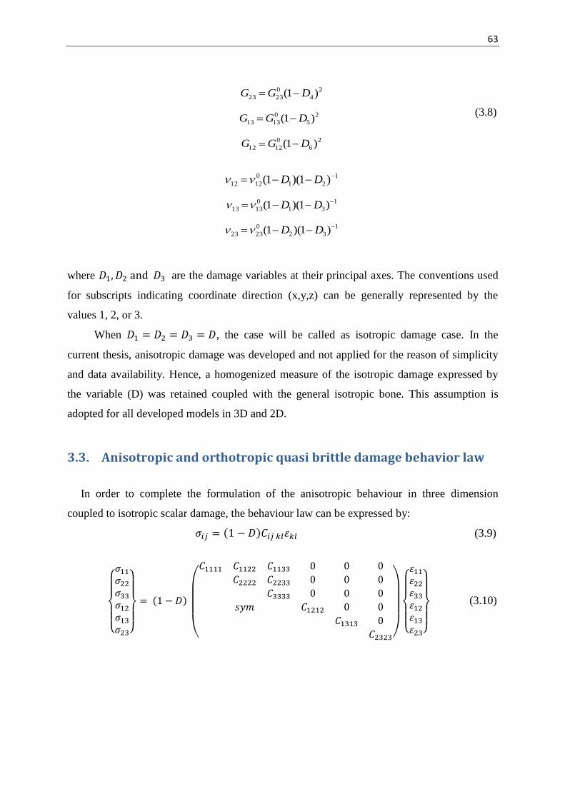
63
24
02323 )1( DGG
25
01313 )1( DGG (3.8)
26
01212 )1( DGG
121
01212 )1)(1( DD
131
01313 )1)(1( DD
132
02323 )1)(1( DD
where are the damage variables at their principal axes. The conventions used
for subscripts indicating coordinate direction (x,y,z) can be generally represented by the
values 1, 2, or 3.
When , the case will be called as isotropic damage case. In the
current thesis, anisotropic damage was developed and not applied for the reason of simplicity
and data availability. Hence, a homogenized measure of the isotropic damage expressed by
the variable (D) was retained coupled with the general isotropic bone. This assumption is
adopted for all developed models in 3D and 2D.
3.3. Anisotropic and orthotropic quasi brittle damage behavior law
In order to complete the formulation of the anisotropic behaviour in three dimension
coupled to isotropic scalar damage, the behaviour law can be expressed by: (3.9)
(3.10)

64
where: And is defined as :
(3.12)
the restrictions on the elastic constants due to material stability are:
In the current work, the elasticity matrix coefficients were expressed in terms of
engineer’s constants defined in simple uniaxial stress conditions. This leads to a formulation
of Hooke’s law for the orthotropic plane-stress case assigned for model B and model test-II:
(3.14)
Young’s modulus, shear modulus and Poisson’s ratio are totally independent in the
orthotropic case and have to be measured separately.
Quasi-brittle damage growth depends on a damage loading function in terms of the
strain components. The growth of the damage variable is controlled by the damage threshold
parameter ( ), which is defined as the maximum of the equivalent strain measure ( )
reached during the load history [Mazars and Pijaudier-Cabot, 1996]:
(3.15)
(3.11)
(3.13)

65
The loading function of damage is expressed by Mazars and Pijaudier-Cabot [Mazars
and Pijaudier-Cabot, 1996]: (3.16)
where is the initial value of when damage starts. If the loading function (f) is negative,
damage does not develop. During monotonic loading, the parameter grows (it coincides
with ) and during unloading and reloading it remains constant: : No damage growth and the material behavior is elastic. : Damage growth and reduction of the stiffness.
Numerous studies have shown that the damage threshold strains of compact bone tissue
are different in tension and compression [Keaveny et al., 1999, 2001, Currey, 2002, Kotha
and Guzelsu, 2003]. All microdamage parameters showed an increase with increasing strain
(Figure 3.2). Regions of cross-hatching and bone fracture are seen more frequently in highly
strained specimens. The extent of damage across the trabecular thickness also increased with
increasing strain [Arthur Moore and Gibson, 2002].
Figure 3. 2 Breakdown of number of damaged trabeculae, normalized by section area, by damage pattern for each strain level [Arthur Moore and Gibson, 2002].
With referring to the relation observed experimentally by [Arthur Moore and Gibson,
2002] for both the experimental law and the dependence of damage growth on the hydrostatic
pressure, a quasi-brittle damage law can be expressed in principal directions by:
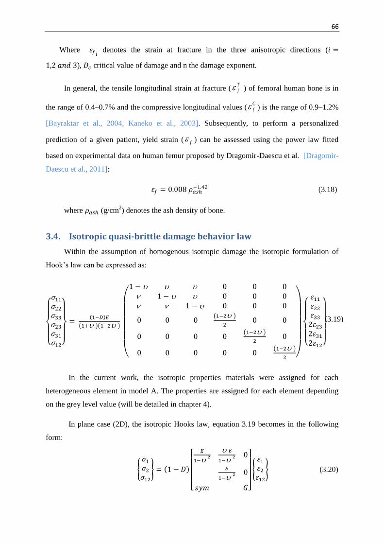
66
Where denotes the strain at fracture in the three anisotropic directions ( ), critical value of damage and n the damage exponent.
In general, the tensile longitudinal strain at fracture (Tf
) of femoral human bone is in
the range of 0.4–0.7% and the compressive longitudinal values (Cf ) is the range of 0.9–1.2%
[Bayraktar et al., 2004, Kaneko et al., 2003]. Subsequently, to perform a personalized
prediction of a given patient, yield strain (f ) can be assessed using the power law fitted
based on experimental data on human femur proposed by Dragomir-Daescu et al. [Dragomir-
Daescu et al., 2011]:
(3.18)
where (g/cm2) denotes the ash density of bone.
3.4. Isotropic quasi-brittle damage behavior law
Within the assumption of homogenous isotropic damage the isotropic formulation of
Hook’s law can be expressed asμ
In the current work, the isotropic properties materials were assigned for each
heterogeneous element in model A. The properties are assigned for each element depending
on the grey level value (will be detailed in chapter 4).
In plane case (2D), the isotropic Hooks law, equation 3.19 becomes in the following
form:
(3.20)
(3.19)

67
As mentioned above, isotropic quasi brittle damage law, bases on above equations, will
be used in its flowing form:
where denotes the strain at fracture.
This newly developed coupled approach can be used to simulate femur failure as well as
fracture patterns in 3D and 2D FE simulations. It can be also used to investigate the effect of
bone property assignment “isotropic and orthotropic” on the predicted fracture pattern.
3.5. Material properties assignment
3.5.1. Anisotropic /orthotropic material properties assignment
Bone material is anisotropic and inhomogeneous due to its varying architecture and
composition of its constituents [Yang et al., 1999]. The determination of the elastic constants
of trabecualr bone by conventional mechanical test procedures is very difficult due to the
small size of specimens of human trabecular bone. In general, compressive tests are applied to
the trabecular sample leads to inaccuracy of the measurements. Yang et al. [Yang et al.,1999],
investigated a data bases consisting of 141 human cancellous bone specimens reported
previously by Van Rietbergen et al. [Van Rietbergen et al.,1996 ] and Kabel et al. [Kabel et
al.,1999]. The data analysis method permits the identification of the elastic constants of
trabecular bone as a function of volume fraction (BV/TV).
In the current thesis, anisotropic mechanical properties are used for the homogenous
model (Model test-II). The properties are estimated as a function of (BV/TV). This arbitrary
choice was adopted to preliminary testing the capability of our proposed model to predict the
fracture failure as well as fracture patterns. Based on the equations proposed by Yang et al.,
[Yang et al., 1999], the final result is the solid volume as a function of volume fraction
dependent orthotropic Hooke’s law for cancellous bone in the form (with correlation
coefficient of 0.934):
(3.22)

68
where bone volume fraction is assumed to be equal to 30% [Keyak and
Falkinstein, 2003], Et = 48.17 MPa [Yang et al., 1999] The anisotropic properties of bone
estimated were calculated by using equations 3.22, 3.23 and 3.24 and are provided in Table
3.1.
Table 3. 1 Estimated anisotropic Material properties.
properties Source General properties
%30BT
BV
MPa17.48Et
[Keyak and Falkinstein, 2003, Yang et al., 1999]
Elastic properties (femur and acetabulum)
E1 = 6840 MPa E2 = 4380 MPa E3 = 2524 MPa
12 =0.19
23 =0.27
31 =0.22
G12= 2159 MPa G23= 1423 MPa G31= 1101 MPa
Estimated based on [Keyak and Falkinstein, 2003, Yang et
al., 1999]
Material properties for bone used for the orthotropic simulation: model test-II was
considered as E3 = E2 = 4380 MPa. For model B, equations, proposed by Baca et al. [Baca et
al., 2008] mentioned in Table 2.1, were applied.
3.5.2. Isotropic material properties assignment
Hook’s laws in the form mentioned in equations 3.19 and 3.20 were applied for each
element in the heterogeneous Models A and C and for the homogenous Model test-I.
(3.23)
(3.24)

69
Material properties assigned for these models are shown in Table 3.2.
Table 3. 2 Material properties used for the isotropic simulation: Models A and test I
General parameters Notation Femur Acetubulum Source Elastic modulus E (GPa) 8.0 20.0 [Keyak and Falkinstein, 2003] Poisson ratio 0.3 0.3 [Keyak and Falkinstein, 2003]
As mentioned above, isotropic quasi brittle damage law is applied in all developed
models. The models parameters used for damage are shown in Table 3.3:
Table 3. 3 Damage law parameters used for femur in the isotropic simulation [Hambli et al., 2012].
Damage law parameters reference Damage properties (femur only)
n
2.0
TcD 0.95
CcD 0.5
[Arthur Moor and Gibson, 2002, Bayraktar et al.2004, Hambli,2001]
o 0.2 %
Tf 0.66 %
Cf
1.2 %
In the current work, we implemented a practical method into ABAQUS/Standard code
(User UMAT Subroutine) to represent fracture by the so-called “kill element” technique
[Hambli et al., 2012]. When the damage parameter reaches a critical value (Dc) inside an
element, the element mechanical contribution to the stiffness matrix is set to zero leading to
the redistribution of the stress state in the crack tip. Once a crack is initiated the propagation
direction is simulated by the propagation of the broken elements of the mesh. An overview of
this approach is illustrated in Figure 3.3.

70
Figure 3. 3 Schematic diagram of the proposed simulated crack propagation implemented in UMAT user subroutine based on both isotropic and orthotropic behaviour laws coupled to quasi-brittle damage.
3.5.3. Orthotropic direction assignment
It has been established that trabecular bone exhibits orthotropic behavior with three
orthogonal directions [Reilly et al., 1974, Van Rietbergen et al., 1996]. Limited number of
studies considered the anisotropic behavior of bone tissue [Fenech and Keaveny, 1999,
Hambli, 2010] due mainly to the difficulty to assign the anisotropic material parameters
related to the local directional material anisotropy.
From a point of view of CDM, there is no difference between crack initiation and
propagation. Both results from the failure of an element with a characteristic dimension
(typical size of a crack). Thus, crack initiation and propagation are studied as unified
approach [Lemaitre, 1985].

71
The assignment of local orthotropic directions and orthotropic properties for every FE
of the mesh is performed in four steps, Figure 3.4 [Hambli et al., 2012]:
Initial conditions : x0 and y0 are the initially assigned reference coordinates (material
directions) of every FE (i) of the femur mesh,
Orthotropic directions computation: performed a 2D elastic analysis under a gait
cycle with a displacement of 15 mm applied to the acetabulum with an orientation of
20° from the vertical.
Assignment of local anisotropic directions: compute the principal stress directions
(xi and yi) for every FE (i)) corresponding respectively to the directions of the
maximum elongation and its orthogonal direction.
Figure 3. 4 Assignment of orthotropic directions and corresponding material properties [Hambli et al., 2012].
The orientations (xi, yi) are stored for every FE in a results file. (xi) lies along the local
predominant trabecular direction, which is locally the stiffest direction (longitudinal
direction), the second is orthogonal to the first direction and represent the direction of
extrema in stiffness in the local region of the cancellous bone.
Orthotropic properties assignment: the orthotropic bone properties were assigned
automatically to each FE (reduced integration) of the femur mesh corresponding to the
computed local directions (xi) and (yi).
For resuming the using of the proposed coupled approach in the current models, the
depicted diagram shown in Figure 3.5 represents the following developed models:

72
- Heterogeneous models:
o 3D FE model (model A): isotropic behavior law coupled to quasi-brittle
damage.
o 2D FE model (models B): orthotropic behavior law coupled to quasi-brittle
damage.
o 2D FE model (model C): isotropic behavior law coupled to quasi-brittle
damage.
These models are used to achieve the objectives of the current thesis.
- Homogenous models:
o 2D FE model (model test-I): isotropic behavior law coupled to quasi-brittle
damage.
o 2D FE model (models test-II): orthotropic behavior law coupled to quasi-brittle
damage.
The purpose of the homogenous models, as we will see in section (3.6), is to preliminary
test the fracture failure calculations and fracture patterns.
These models are proposed to simulate the proximal femur fracture under both
configurations: single limb stance and sideways fall configurations.
The following section will present the applied boundary conditions and loads used for
these two configurations.

73
Figure 3. 5 The developed models of the current study.

74
3.6. Loading and boundary conditions
3.6.1 Loading and boundary conditions of single limb stance simulation in 3D
Boundary conditions were applied to the FE models to represent the conditions of
mechanical testing by performing 3D image registration. In each model, the location of the
applied displacement was extrapolated from the registration coordinates of the contact points
attached to the femoral head which represent in turn the contact between the hip and femur
head.
As kinematical boundary conditions, the femur was assumed to be clamped in the distal
part, Figure 3.6.
Figure 3. 6 An example of 3D FE loading and boundary conditions applied for human femur.
A displacement of 15 mm was imposed on the assumed contact areas between the centre
of the hip joint and femoral head.

75
3.6.2 Loading and boundary conditions of single limb stance configuration in 2D
A FE model was constructed including the proximal femur articulating freely with a
representation of the acetabulum, Figure 3.7. Boundary and loading conditions are chosen
according to the experimental study reported in keyak and Falkinstein, [Keyak and Falkinstein
2003]. The model was loaded by applying displacements incrementally with an orientation of
20◦ from the vertical to the top surface of the acetabulum. The lower surfaces of the proximal
femur were encastred, Figure 3.7. The reaction force applied to the acetabulum was computed
considering the femur cracking versus the displacement of femur head.
Figure 3. 7 FE model: (a) applied boundary conditions in single limb stance configuration.
The appropriate orientation of the resultant hip force was estimated for all femur
specimens. An arbitrary individual hip displacement of 1.5 cm was directed towards the
center of contact between the pelvis and the femoral head.
3.6.3 Loading and boundary conditions of sideway falls simulation in 2D
The boundary conditions applied represented a fall onto the greater trochanter based on
experimental studies reported earlier [Courtney, 1994,1995], see Figure 3.8. The angle
between the femoral shaft and the horizontal was 10° and the femur was internally rotated by
15°.

76
Figure 3. 8 Applied boundary conditions in sideway fall configuration
[de Bakker et al., 2009, Hambli et al., 2013].
The appropriate orientation of the resultant hip force was estimated for all femur
specimens. An arbitrary individual displacement of 1.5 cm was directed towards the greater
trochanter. The surface nodes perpendicular to the resultant hip force on the greater trochanter
were fixed vertically and allowed to displacement in the horizontal direction to simulate
constraints between the femur and a contact surface.
3.7. Validation of the developed quasi brittle damage models
The FE analysis software used in the current study is ABAQUS® 6.7 EF. All laws and
relationships discussed above have been implemented in FORTRAN 90 by means of the
UMAT (User Material) subroutine. UMAT subroutines can be used to define the mechanical
constitutive behavior of a material. They will be called at all material calculation points of
elements at all iterations. The current developed programs were subjected to preliminary
several tests for 2D models test I and II. The following preliminary tests were performed for:
Mesh sensitivity test.
Effect of material property assignments on the fracture pattern.
Damage nucleation.
Fracture propagation.
Identical boundary and loading conditions were chosen as imposed in the experimental
study of Keyak and Falkinstein [Keyak and Falkinstein 2003].
3.7.1 Preliminary validation of the femur fracture model
To demonstrate the potential of this validation, a left proximal femur of a male (age 61)
referred as Model test-I and test-II was loaded until failure under one-leg stance. The model
was investigated by keyak and Falkinstein [Keyak and Falkinstein, 2003].

77
Due to the non-availability of 2D human femur specimens, a validated homogenous
model was used. The 2D contour of the femur was digitized based on the geometry of the
model investigated by Keyak and Falkinstein, Figure 3.9. A FE model was constructed
including the proximal femur and acetabulum. Boundary and loading conditions simulated the
experimental setup, reported in keyak and Falkinstein, was applied [Hambli et al., 2012]. The
distal portion had a zero displacement condition (Figure 3.9) and a displacement of 15 mm
was applied on the proximal femur with an angle of 20◦ from the vertical. The mechanical
properties of bone used for this simulation were compiled in Tables 3.1, 3.2 and 3.3.
Figure 3. 9 FE mesh for the femur and the acetubulum.13150 four-nodes quadratic elements [Hambli et al., 2012]. The arrows represent the direction of the hip displacement.
The main purpose of this test, as mentioned above, was only to examine the
applicability of the current developed 2D model for prediction of fracture location.
3.7.2 Evaluation of mesh sensitivity
To investigate the sensitivity of the femur structure responses and fracture pattern on the
FE mesh size, sensitivity studies were conducted to quantify the effects of variations in mesh
size on the 2D model-predicted reaction force–displacement relationship and proximal femur
fracture locations as well as the fracture pattern. Overall, ten different mesh sizes, Table 3.4,
defined by a global element size for the edges ranging from 0.25 to 2.5 mm were employed,
generating 1000 to 20000 elements.
Table 3. 4 Different mesh sizes used for the evaluation of mesh sensitivity.
Mesh label m01 m02 m03 m04 m05 m06 M07 m08 M09 M10
Mesh size, mm 0.25 0.5 0.75 1.0 1.25 1.5 1.75 2.0 2.25 2.5

78
The curves of reaction forces versus the imposed displacements ar presented in Figure
3.10.
Figure 3. 10 Reaction force versus vertical displacement, using ten different FEM meshes: finest mesh is labeled m01, coarsest mesh is labeled m10.
It was found that the models converged at element size in the range of 0.5 to 1.5 mm, on
the contrary, at element size of 2.5 mm, the element stiffness presents a significant
divergence.
Mesh size
Applied displacement
at 1.1 mm at 4.37 mm at 5.75 mm
m01
m05
m10
Figure 3. 11 Crack propagation (crack profile) in the course of the simulation at different instants for three different mesh sizes.

79
Figure 3.11 depicts some examples of the obtained crack profiles taken at three different
instants: just before crack initiation, at crack initiation and just before complete separation of
femur fracture. Only three representatives of ten mesh sizes were presented. The finest
element size, 0.25 mm (m01), the middle (m05) and the coarsest one (m10). A distinct
variation of the crack propagation and the volume left intact is evident from Figure 3.11.
Examination of the damage under compression loads in single limb stance of human
femur head is presented in Figure (3.12). It shows that damage in the tensile zone near the
greater trochanter has not suffered from high strains. Only the compressed lower neck side
featured a significant damage which is concentrated at the basal zone area. However,
elements with D ≥ 0.5 were deleted. As expected, the coarser the mesh, the more volume is
affected by damage as shown in Figure 3.12 and thus, the width of the remaining bone
material linking the femoral head to the femur is reduced.
Mesh size
Applied displacement
at 1.1 mm at 4.37 mm at 5.75 mm
m01
m05
m10
Figure 3. 12 Damage accumulations at different instants for three different mesh sizes.

80
As shown from Table 3.5, the peak value and the profile of the reaction force is little
affected by the mesh size, the failure loads obtained were 2649,3 ± 194,04 N (discrepancy of
7.3) at fracture displacement of 5.244 ± 0.624 mm (discrepancy of 11.8%).
Table 3. 5 Resulted maximum facture force at 10 different mesh sizes (m01 to m10)
and displacement (at crack intiation and complete fracture).
No. of elements in femur
Force (N) maximum
Displacement (mm) at end of linear range at max. force when force drops abruptly
m01 94148 2613 2,56 5,03 5,03 m02 23128 2812 2,9 5,21 6,13 m03 10380 2940 2,9 5,44 6,13 m04 5840 2767 2,9 5,44 6,59 m05 3712 2809 2,86 4,47 6,54 m06 2541 2708 2,86 4,23 6,31 m07 1938 2600 2,71 6,38 8,44 m08 1432 2400 3,03 4,95 7,28 m09 1223 2333 4,79 5,48 6,86 m10 950 2511 2,71 5,81 8,56
Generally, except for the coarsest mesh size (m10), the current model proved almost
insensitive to mesh size. For an optimal balance between computational cost and precision,
we chose an element size of 0.25 mm to mesh the homogeneous femur to investigate the
effect of isotropic and orthotropic material assignement for the 2D quasi brittle damage
model.
3.7.3 Effect of material assignment on two dimensional femur fracture pattern
As shown in Figures 3.13a-d, with isotropic behavior under excessive load deformation,
the overall maximum stress started at the inferior cortex of the femoral neck. The evolution of
the crack is initiated at the inferior cortex at an imposed displacement value of 1 mm. The
crack then expands upwards, following an inclined path towards the upper surface resulting in
a complete separation of the proximal femur.
In contrast, with orthotropic behavior, Figures 3.13e-h, the crack is initiated at the lower
compression side, Figure 3.13e, and later separately at the tension side, propagates slowly
then bifurcated into two directions towards the upper tensile side of the femoral neck.

81
Displ.= 1 mm Displ.= 2 mm Displ.= 2.75 mm Displ.= 3.5 mm F
ract
ure
(I
sotr
op
ic b
ehav
ior)
(a)
(b)
(c)
(d)
Fra
ctu
re
(Ort
ho
trop
ic
beh
avio
r)
(e)
(f)
(g)
(h)
Figure 3. 13 Crack propagation in a homogenous human femur, mesh size (1 mm). Upper row: homogenous isotropic, lower row: homogenous anisotropic [Bettamer et al., 2012a].
At a displacement of 2.75 mm, crack is initiated close to the greater trochanter at the
upper tension side, (Figures 3.13f and 3.13g), grows rapidly towards the lower compression
side resulting in the complete separation of the proximal femur in the form of basicervical
fracture at a displacement of 3.5 mm (Figure 3.13h).
The aim of this point of investigation is to test the ability of the proposed model to
predict fracture profile depending on the femur head displacement (Figure 3.13). The results
show that our coupled approach can be used to predict the progressive fracture profile through
varying the material properties.
3.8. Conclusion
2D and 3D FE simulations models were presented in the current chapter. These models
were based on isotropic /orthotropic behavior laws coupled to quasi-brittle damage. The 2D
model was preliminary validated by using the right adult human femur model previously
investigated by Keyak and Falkinstein and simulated until complete fracture under one-legged
stance load. Mesh sensitivity of the current model was evaluated and the concept of coupled
damage was introduced. A series of experiments will be presented in the following chapter
which will be used to validate the proposed damage models.

82
83
Chapter 4
Experimental Work
Abstract
The experimental work will permit to validate the proposed finite element
(FE) models. At the first, the current chapter presents the description and the
preparation of the femur specimens used in the experimental part. The steps
concerning the image segmentation as well as the data extraction from XCT and
DXA images to generate finite element meshess will be described. Subsequently, a
review of the experimental investigation under limb stance configuration, femur
specimen testing will be presented. This configuration has been demonstrated, in
previous studies, the ability to reproduce the observed clinical fractures. A totally
original validation procedure in the case of femur deformation is developed
based on 2D and 3D Digital Image Correlation (DIC) method. Finally the
validation of the designed single limb stance assembly will be introduced.
Résumé
L’approche expérimentale permettra de fournir des données afin de valider les résultats obtenus par les modèles numériques. Dans un premier temps, ce
chapitre présentera la description et la préparation des échantillons des fémurs
utilisés dans la partie expérimentale. Les étapes concernant la segmentation des
images ainsi que l'extraction des données à partir des images XCT et DXA pour
générer des maillages éléments finis seront décrites. Par la suite, un état de l’art, sur les études expérimentales précédentes, sous la configuration d’appui monopodal et les essais réalisés dans le cadre de cette étude seront présentés.
Cette configuration a été choisie car elle a démontré, dans des études
précédentes, sa capacité à reproduire les fractures cliniques observées. La
méthode de corrélation d'images numériques (en 2D et 3D) totalement nouvelle
pour le cas de déformation du fémur sera utilisée. Enfin, une validation du
dispositif de l’appui monopodal conçu à l'aide de fémur bovin sera introduite.

84
4.1. Introduction
Experimental approach comparing with Finite Element (FE) method predicted results,
can provide comprehensive predication of mechanical properties and load that leads to failure
of neck femoral. For this reason, the objective of the experimental branch in current work is to
validate our predicted numerical results.
To introduce the experimental part of the current work, we will start by describing firstly,
the steps of specimen preparation, data acquisition from Dual X-ray Absorptiometry (DXA)
and X-ray Computed Tomography (XCT) and the steps of meshing the FE models which are
used in the current work. Secondly, a review of single limb stance experiments is presented,
the current designed experimental device and testing protocol will be introduced. Finally, the
mechanical compression testing, loading conditions and assembly validation test will be
discussed.
4.2. Femur specimens
In the current work, we used human femur bone to validate the proposed FE models and
bovine femurs for validation tests of the designed fixture assembly. Ten human cadaveric
femurs were obtained (7 women and 3 men, aged 85.9 ± 10.75 years, range 62–100 years)
were purchased from the Institute of Anatomy (University of ParisV, Paris, France). In order
to ensure disease-free specimens, for each specimen, a routinely certificate of non-
communicable disease was issued by a hospital doctor. Serology for hepatitis C, HIV,
HTLV1, HTLV2 was made before the acquisition. Eight specimens will be experimentally
tested under axial load compression under single limb stance configuration.
4.2.1 Femur specimens preparation
The length of all human femur received was ranged from 167 mm to 207 mm. Each
femur was cut transversely to a maximum length of 120 mm (scaning size limits) beyond the
lesser trochanter to the head femoral as shown in Figure 4.1. This dimension has been chosen
taking into account the space availability in the different devices that will be used later.

85
Figure 4. 1 Some samples before testing.
Freshly drawn femurs were wrapped between all processing steps in a cloth soaked in
saline (NaCl 0.9%) in order to avoid dehydration. Prior to degreasing, each specimen was
marked with a label carrying the date and time of bleaching. Then the femur specimens were
immersed in hot water (see Figure 4.2) at a temperature of 85°C by using a thermometer to
regulate the temperature. A bleaching agent of 30 ml was poured in the container.
Subsequently, the specimens were boiled for two hours and defatted softly, without causing
any damage to the bone. This degreasing was done to avoid fat-melting during scan
operations which last hours and cause an increase in temperature. This operation was repeated
twice for each specimen after cooling between two stages. The specimens were then allowed
to cool to room temperature in the container and finally stored in the refrigerator at 4° C.
Figure 4. 2 Degreasing process of human femur specimens.
Then, in vitro Dual X-Ray Absorptiometry (DXA) scans of the femurs were obtained
with a Hologic QDR 4500 scanner (Hologic Inc., Waltham, USA) using the standard protocol

86
for the proximal femur. Standard positioning was used across all specimens, and the proximal
femoral and neck areal Bone Mineral Density (BMD) was evaluated with the software
provided by the manufacturer (Table 4.1).
Table 4. 1 Measured total and neck femoral densities for human femur specimens.
Femur ID Weight R/L Age Sex BMD Neck, g/cm2
BMD Total, g/cm2
A 235.0 Left 62 Male 0,41 0,64 B 244.0 Left 98 Female 0,45 0,72 C 276.0 Right 85 Female 0,50 0,75 D 273.0 Left 85 Female 0,48 0,68 E 378.0 Right 91 Female 0,75 0,83 F 388.0 Left 91 Female 0,79 0,86 G 244.0 Left 98 Female 0,49 0,62 H 271.0 Right 80 Male 0,43 0,53 I 277.0 Left 80 Male 0,44 0,61 J 263.0 Left 87 Female 0,51 0,68
In order to study the effect of femur geometry on failure loads of proximal femur,
different geometrical parameters of all femur specimens were taken using ABAQUS
measuring commands. As shown in Figure 4.3 the following parameters are measured:
femoral neck axis length (AB), femoral head diameter (CD), femoral neck width (EF),
cervical-diaphyseal angle (H), trochanteric-diaphyseal diameter (IJ), diaphyseal diameter
(KL), and length of femur specimen (L1) and the diaphseal length (L2). These physical
measurements are compiled in Table 4.2.
Figure 4. 3 Definition of the parameters measured for femur specimens [modified from: Bonnet et al. 2007].

87
Table 4. 2 Physical dimensions measured for human femurs, mm.
4.3. Image acquisition
Image acquisition is the first process concerning the generation of mesh models. This
process is performed by using DXA to generate 2D FE model and XCT to generate 3D FE
model.
These non-invasive techniques have gained considerably in importance due to
continuous improvements in X-ray tubes and XCT devices. These systems are based on the
property that X-ray beams satisfy differently in bone and soft tissues as a function of photon
energy [Testi et al., 1999]. They can achieve resolutions down to 1 µm. Besides, they enables
the generation of accurate FE models for the human femur [Keyak et al., 1998, Cody et al.,
1999].
4.3.1 Image Segmentation
Prior to simulating the mechanical properties of the femur, the images are usually
segmented for the different phases of the femur to be identified. This process consists of the
extraction of outer surface in 3D or outer contours in 2D. The segmentation process consists
in partitioning the 3D image voxels into distinct parts based on their grey level values. The
segmentation process consists of three main operations: filtering, binarisation and correction
[Aufort et al., 2007].
4.3.1.1 Data from DXA
In order to identify our FE models, computer codes were applied by introducing data
base form DXA and XCT. These codes were achieved in collaboration with Dr. Rozenbaum’s
group at the ISTO (Institute des Sciences de la Terre d’Olréans).
Femur ID AB CD EF H,deg IJ KL L1 L2
A 85,12 42,30 30,69 126,00 34,76 27,20 167,00 88,50 B 86,10 42,12 29,83 132,00 31,70 28,15 167,00 86,50 C 90,20 44,25 31,52 129,50 32,60 29,10 187,00 106,70 D 90,02 45,70 31,20 129,00 30,40 29,00 184,00 105,70 E 104,93 50,60 39,89 129,50 34,35 31,10 193,00 94,25 F 104,70 50,10 39,16 132,00 36,10 32,20 184,00 97,50 G 103,44 46,10 32,97 118,00 34,14 30,06 175,00 80,10 H 95,41 43,40 32,56 122,50 33,60 27,40 207,00 108,00 I 107,05 50,30 35,15 117,50 33,90 31,90 193,00 104,10 J 96,68 42,80 31,87 128,50 31,70 28,80 184,00 96,80

88
First the contour of each image was identified. The images were imported into the
MATLAB software. The images were detected after performing several operations like edge
dilation the boundary.
The true color image was converted to a grey-scale image (which carries the image
intensity information) and used for calculating the density (Figures 4.4a and 4.4b).
(a) (b) (c)
Figure 4. 4 (a) DXA of a proximal femur specimen (b) Grey-scale image obtained from the DXA scan data set of an artificial composite femur (c) contour extraction.
The gray value of each pixel was converted into density of that pixel. A linear
correlation was assumed between pixel value and density [Schileo et al., 2008]. As part of the
data extraction, Young’s modulus was correlated to the density using an exponential
correlation, shown in Table 2.1, developed by Keyak and Falkinstein [Keyak and Falkinstein,
2003]. Finally the projected 2D hetergenous FE model compatible for ABAQUS/Standard
code were created.
4.3.1.2 Data extraction from XCT images
In order to localize and determine the volume of interest concerning a selected femur,
a segmentation technique was applied. This process has been implemented in collaboration
with Dr. Rozenbaum’s group at the ISTO laboratory of CNRS-Orléans and Prof. Jenanne’s
group at the PRISME laboratory of the University of Orléans. Images were obtained using the
Skyscan 1072 high-resolution µCT. The X-ray source was set at 80 kV and 100 µA, and the
magnification was set so as to obtain a pixel size of 50 µm. A 1024_1024 12-bit digital
cooled CCD coupled to a scintillator was used to record the radio-graphic projections. A total
of 209 projections were acquired over an angular range of 180° (angular step of 0:9°).

89
This technique was achieved into three steps: filtering, binarization and correction.
Filtering
The acquired real images are usually noisy, and the noise level highly depends on the
quality of the imaging system. In this work, a standard median 333 filter was applied in
order to reduce possible artifacts such as impulsive noise.
Binarisation
The filtered images were binarized in order to separate bone voxels from pore voxels. A
standard binarisation method was applied. In this method, a threshold defined as the local
minimum between the two maxima of the histogram of the filtered image was first
determined. Then, voxels whose grey levels were below this threshold are considered as pore
voxels. The remaining ones were considered as bone voxels.
Correction
After the binarisation step and in order to take into account the anatomical constraints of
porous objects, a correction step was applied. Since, all trabeculae of bone tissues are
interconnected; the binarised image was verified to ensure the existence of only one
connected structure (see Figure 4.5). For this purpose, the Hoshen-Kopelman’s clustering
algorithm was used [Hoshen and Kopelman, 1976]. Using HK algorithm, each group is
assigned a distinct label. The principal (largest) cluster is kept and voxels of the other smaller
clusters are considered as pore voxels.
Figure 4. 5 Image segmentation: correction step.
A 3D segmentation software developed at the ISTO was used to automatically
identifying cortical and trabecular components of the proximal femur and isolated from the
environment in which the bone was scanned (water and air). The values of the voxels are
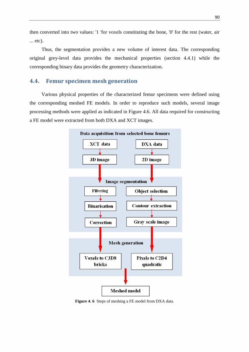
90
then converted into two values: '1 'for voxels constituting the bone, '0' for the rest (water, air
... etc).
Thus, the segmentation provides a new volume of interest data. The corresponding
original grey-level data provides the mechanical properties (section 4.4.1) while the
corresponding binary data provides the geometry characterization.
4.4. Femur specimen mesh generation
Various physical properties of the characterized femur specimens were defined using
the corresponding meshed FE models. In order to reproduce such models, several image
processing methods were applied as indicated in Figure 4.6. All data required for constructing
a FE model were extracted from both DXA and XCT images.
Figure 4. 6 Steps of meshing a FE model from DXA data.

91
For 3D FE, the entire proximal femurs structures are modeled using ABAQUS/Standard
code, element types of C3D8 (8-node quadratic brick). Each voxel of femur structure is
converted to a FE. These conversions produce accurate geometrical models and allow
modeling the complex porous structures of the trabecular bone.
Table 4.3 compiles the human femurs along with the spatial resolution used in the
current 3D simulation.
Table 4. 3 Human femur resolution and dimensions used in the current simulations.
Human Femur
Type of Mesh
Dimensions (voxels)
Dimensions (mm)
A C3D8 168 × 260 × 94 8.40 × 13.000 × 4.700 B C3D8 180 × 260 × 93 9.00 × 13.000 × 4.650 C C3D8 230 × 268 × 93 11.50 × 13.400 × 4.650 D C3D8 190 × 270 × 92 9.50 × 13.500 × 4.600 E C3D8 180 × 260 × 88 9.90 × 14.300 × 4.840 F C3D8 180 × 260 × 92 9.90 × 14.300 × 5.060 G C3D8 200 × 280 × 87 10.00 × 14.000 × 4.350 H C3D8 190 × 280 × 90 9.50 × 14.000 × 4.500 I C3D8 200 × 260 × 97 11.00 × 14.300 × 5.335 J C3D8 190 × 275 × 100 10.45× 15.125 × 5.500
4.4.1 Relation between grey level and mechanical properties
The porous body formed by a complex network of bone trabeculae has particular
mechanical properties, which are determined not only by their porosity, but also by the
arrangement of trabeculae in the 3D space. In the current work, each femur specimen, cortical
and trabecular bone tissue were identified based on the number of elements in a fixed
neighborhood. Each element was assigned a Poisson's ratio of 0.3 and an isotropic Young's
modulus that depends on tissue type according to the CT gray value using the empirical
equations mentioned above in chapter (2), Table 2.1.
For each voxel, elastic modulus was computed from the ash density of bone ( using the following correlations for both trabecular and cortical bone [Keyak and Falkinstein,
2003] :
If then the CT scan voxel element was considered as trabecualr bone and
its elastic mouduls (in MPa) was calculated by using the following emperical equation: (4.1)

92
If then the CT scan voxel element was considered as bone in a
transition phase (between trabecular and cortical) and its elastic modulus (in MPa)
was calculated by using the following equation:
If then the voxel element was considered as cortical bone and its elastic
mouduls (in MPa) was calculated by using the following emperical equation:
The ash density (in g/cm2) for each CT scan voxel was computed from the calibrated
CT scan data, [Keyak and Falkinstein, 2003]: =
4.5. Femur specimen testing
In vivo, the femoral neck may undergo different loads. Compressive load through the
femoral head acts through a significant moment arm (the length of the femoral neck), which
causes large bending loads on the femoral neck [Browner et al., 2009].
In vitro, femur bone has been subjected to all these experimental tests in order to
investigate and to assess common daily fractures. However, the most common cause of long
bone fractures due to torsion and bending forces occurs, in vivo, in the central third of the
shaft [Bramer et al., 1998] which is out of the scope of the current research. We are interested
in femoral neck fractures. We believe that the activity and loading on a relatively unprotected
hip are the most likely causes of fractures and leads to considerable mortality.
Hence, the main objective in the current work is to assess the femoral neck fracture
under one-legged stance loads. This evaluation is necessary to study the incidence of
spontaneous fractures [Cristofolini et al., 2007] and the behavior of the hip during daily
activities [Juszczyk et al., 2011].
4.5.1 Single limb stance test
Some studies have conducted tests with a femoral shaft parallel to the vertical where the
proximal femur is mainly subjected to shear [Beck et al., 1990, Esses et al., 1989, Lochmüller
(4.2)
(4.3)
(4.4)
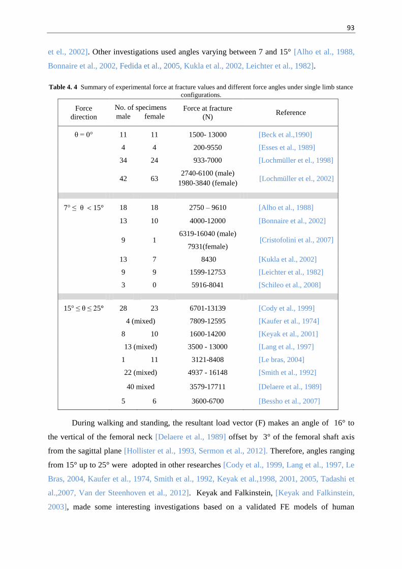
93
et el., 2002]. Other investigations used angles varying between 7 and 15° [Alho et al., 1988,
Bonnaire et al., 2002, Fedida et al., 2005, Kukla et al., 2002, Leichter et al., 1982].
Table 4. 4 Summary of experimental force at fracture values and different force angles under single limb stance configurations.
Force direction
No. of specimens Force at fracture (N)
Reference male female
θ = 0° 11 11 1500- 13000 [Beck et al.,1990]
4 4 200-9550 [Esses et al., 1989]
34 24 933-7000 [Lochmüller et el., 1998]
42 63 2740-6100 (male)
1980-3840 (female) [Lochmüller et el., 2002]
7° ≤ θ 15° 18 18 2750 – 9610 [Alho et al., 1988]
13 10 4000-12000 [Bonnaire et al., 2002]
9 1 6319-16040 (male)
7931(female) [Cristofolini et al., 2007]
13 7 8430 [Kukla et al., 2002]
9 9 1599-12753 [Leichter et al., 1982]
3 0 5916-8041 [Schileo et al., 2008]
15° ≤ θ ≤ 25° 28 23 6701-13139 [Cody et al., 1999]
4 (mixed) 7809-12595 [Kaufer et al., 1974]
8 10 1600-14200 [Keyak et al., 2001]
13 (mixed) 3500 - 13000 [Lang et al., 1997]
1 11 3121-8408 [Le bras, 2004]
22 (mixed) 4937 - 16148 [Smith et al., 1992]
40 mixed 3579-17711 [Delaere et al., 1989]
5 6 3600-6700 [Bessho et al., 2007]
During walking and standing, the resultant load vector (F) makes an angle of 16° to
the vertical of the femoral neck [Delaere et al., 1989] offset by 3° of the femoral shaft axis
from the sagittal plane [Hollister et al., 1993, Sermon et al., 2012]. Therefore, angles ranging
from 15° up to 25° were adopted in other researches [Cody et al., 1999, Lang et al., 1997, Le
Bras, 2004, Kaufer et al., 1974, Smith et al., 1992, Keyak et al.,1998, 2001, 2005, Tadashi et
al.,2007, Van der Steenhoven et al., 2012]. Keyak and Falkinstein, [Keyak and Falkinstein,
2003], made some interesting investigations based on a validated FE models of human

94
proximal femur under single limb stance loads. They used to apply an angle of 20° in their
validated simulations. Picking this arrangement as reference configuration, the same angle
was applied in the current thesis. Table 4.4 represents a summary of the reported in vitro
destructive tests together with the different directions of the applied force in single limb
stance and the obtained failure loads.
4.5.2 Measuring methods used to measure bone deformation
Mechanical in vitro testing of bones is often used on cadaveric human studies in order
to evaluate the failure locations. Some parts of the human body have complex geometries
such as the proximal femur. The deformation of such geometry when subjected to axial loads
requires an accurate measuring tool able to capture the deformation of such complex
geometry deformation. The simplest mode of gathering displacement values by the machine
LVDT has several essential advantages. The measurement of the actual deformation in the
sample is much more intricate, since the measured deformation is not uniquely related to the
actual deformation of the specimen.
Strain measurements from bone surfaces can be achieved by using several
applications. Although various strain measurement methods such as photoelasticity,
holographic interferometry and brittle coacting have established, the most common is electric
resistance strain gaugesg [An and Draughn, 2000].
While it is possible to use strain gages, their major disadvantages impose rigorous
limitations on the strain value that can be applied to the sample. However, strain gauges
measurements of bone deformation are frequently applied in bone mechanics and often used
for validation purposes in computer models [Yosibash et al., 2007]. Lotz et al. [Lotz et al.,
1991a,b] used the data obtained by strain gauges to validate their simulation model of
proximal femur. Composite synthetic models are also tested and strain gages were applied to
assess local deformations [Cristofolini et al., 1996]. When strain gauges are applied, they need
to be firmly glued onto the material. It must be assumed to undergo the same deformation as
the material without affecting the stiffness. Even if using a large number of strain gages, they
do not provide sufficient spatial resolution nor 3D components of strain distributions in zz, xy
or xy directions [Yang et al., 2011], thereby risking misinterpretation and large experimental
errors [Yosibash et al., 2007].
95
Besides the restriction to one single spot, several additional constraints can be cited:
The necessity of a plane and smooth surface to bond the strain gauge.
Technically, the surface for bonding strain gauges should be free from organic
contamination, greases, water proof and sufficiently rough which are almost
impossible to reach these cruel conditions.
The attachment of the strain gauges to the bone surface might stiffen the bone
slightly, resulting in an overestimation of stiffness.
The experiment must be conducted strictly isothermally as temperature effects
are the most common cause of error in application of strain gauges.
In order to overcome the above mentioned limitations, optical methods such as Digital
Image Correlation (DIC) and Digital Speckle Pattern Interferometry (DSPI) have seen
remarkable growth in the recent years. DSPI is also a non-contacting measuring tool like DIC.
Even though DSPI was applied to measure 3D bone strain field [Zhang et al., 2001], the
surface deformation was not evaluated. Later on, DSPI was applied and local surface contour
was evaluated on mouse femora [Yang et al., 2007].
However, due to the relative ease of use and versatility of the methods, the use of 2D-
DIC and 3D-DIC becomes widespread in measuring the surface displacements.
2D-DIC was used to study the local distributions of mechanical strain on a section of
sheep bone callus- a hard bony tissue that develops around the ends of a fractured bone during
healing [Thompson et al., 2007].
3D-DIC has been used earlier for macroscopically strain measurements to determine the
local strain in human cortical bone or at microscopic scale to analyze strain distribution
around a microcrack around osteocyte lacunae in cortical bone [Nicolella et al., 2006]. In
trabecular bone this technique was used to calculate and visualize the local strains in single
trabeculae [Verhulp et al., 2004]. Further studies have applied 3D-DIC method on cartilage
[Zhang et al., 2005], and bone fracture callus [Thompson et al., 2007] in order to measure
their strains under different loads. Recently, Sztefek et al. [Sztefek et al., 2010] have used
sample sections of tissue under conditions directly representative of applied in vivo loading
and used 3D-DIC to measure a murine tibia during compressive loading of the knee joint.
Despite the utility of DIC as a tool in the field of experimental solid mechanics [Tiwari
et al., 2007], to the best to our knowledge, there are no previous studies have applied it to
measure in vitro the 3D surface topology deformation of human cadaver femur.
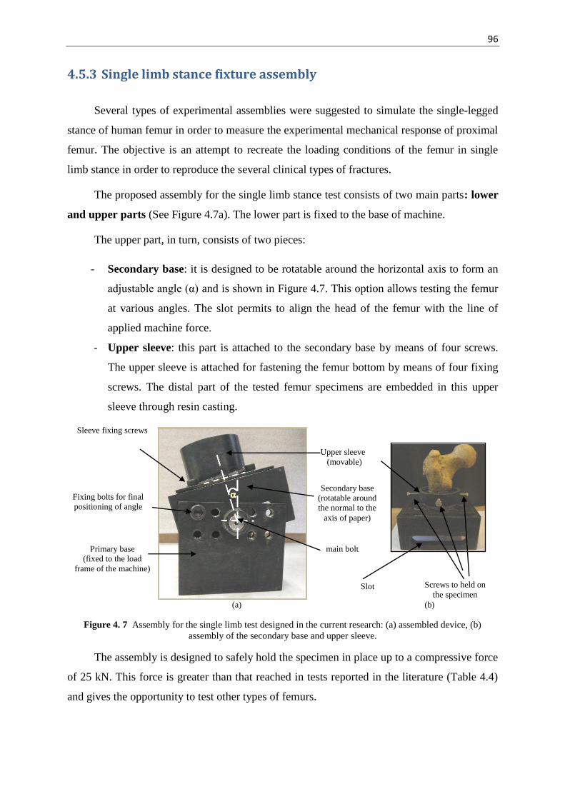
96
4.5.3 Single limb stance fixture assembly
Several types of experimental assemblies were suggested to simulate the single-legged
stance of human femur in order to measure the experimental mechanical response of proximal
femur. The objective is an attempt to recreate the loading conditions of the femur in single
limb stance in order to reproduce the several clinical types of fractures.
The proposed assembly for the single limb stance test consists of two main parts: lower
and upper parts (See Figure 4.7a). The lower part is fixed to the base of machine.
The upper part, in turn, consists of two pieces:
- Secondary base: it is designed to be rotatable around the horizontal axis to form an
adjustable angle (α) and is shown in Figure 4.7. This option allows testing the femur
at various angles. The slot permits to align the head of the femur with the line of
applied machine force.
- Upper sleeve: this part is attached to the secondary base by means of four screws.
The upper sleeve is attached for fastening the femur bottom by means of four fixing
screws. The distal part of the tested femur specimens are embedded in this upper
sleeve through resin casting.
(a) (b)
Figure 4. 7 Assembly for the single limb test designed in the current research: (a) assembled device, (b) assembly of the secondary base and upper sleeve.
The assembly is designed to safely hold the specimen in place up to a compressive force
of 25 kN. This force is greater than that reached in tests reported in the literature (Table 4.4)
and gives the opportunity to test other types of femurs.
Screws to held on the specimen
Upper sleeve (movable)
Sleeve fixing screws
Secondary base (rotatable around the normal to the
axis of paper)
main bolt Primary base (fixed to the load
frame of the machine)
Fixing bolts for final positioning of angle
Slot

97
During testing, four screws held the specimen in a vertical position with respect to the
upper part. They also permit to avoid contact between the femur and the walls of the upper
part without any pressure being excreted on the specimen surface.
The current fixture assembly provides the following advantages:
- The possibility to make different experiments by applying axial loads at different
angles through changing the angle of rotation (α).
- As the upper sleeve is movable, this provides the possibility to fix other sleeves
with different diameters. Hence this device can serve over a wide range of different
femur types up to the maximum design load.
- The slot in the secondary base part gives the possibility to easily align the head of
the femur with the line of interaction of the applied axial compression load of the
testing machine.
4.5.4 Mechanical compression test of single limb stance loading configuration of human femur specimens
The compression test was performed in a singl limb stance configuration. This position
has demonestrated, in previous studies, the ability to reproduce the observed clinical fractures.
The test preparation as well as test conditions are as follows:
(i) The human cadaver femurs were installed in the single limb assembly presented in
Figure 4.7 and maintained in the center of upper sleeve by using the four fixing
screws.
(ii) The distal portion of each femur is fixed by using a casting of epoxy resin
(SICOMIN Epoxy Systems, France) which was prepared by mixing 100g of resine
(SR 1500) with 33g of hardner (SD2505).
(iii) The assembly of fixture and femur is left at room temperature so that the resin
cures (from 4 to 6 hours).
(iv) The fixing screws are loosened upon solidification of the resin and the assemby is
stored at 4°C until performing the compression test.
(v) Three hours before use, the assembly is removed from the refrigerator. Noting that
the fact to cool and removing the femur from the refrigerator have an effect on his
behavior because the bone is a living material. But these necessary steps have been

98
minimized and standardized as possible so as not to alter too much the behavior of
the bone.
(vi) The assembly is mounted on a universal testing machine Instron, equipped with a
load cell of 200 kN (see Figure 4.11) and is oriented within the coronal plane at
20° [Keyak and Falkinstein, 2003, Keyak et al., 2009, Dall’Ara et al.,2013].
(vii) The compressive load is applied with a crosshead speed of 2 mm/min [Heini et al.,
2004].
The displacement of the crosshead is measured with LVDT and is continuously
recorded throughout the test along with the applied force. In order to determine
displacement and the strains fields of the specimens, optical methods are used. Two
optical charge-coupled device cameras (CCD), connected to a computer, were used to
continuously record images of the sample surface during the test. The maximum image
resolution of this camera is 1380×1024 pixels with a 8-bit digitization for grey levels
(28=256 grey levels). The maximum acquisition frequency used is one image per second.
Images are recorded, digitized and stored in a computer as digital images. During the
compression tests, a lamp is installed in front of the samples to illuminate them in order to
not affect the acquisition by the natural light variations in the room. After that, image
processing is performed using the softwares Deftac 3D and 7D-3D [Vacher et al., 1999]
based on the Digital Image Correlation (DIC). The outcome are the displacement fields in
the three directions on the surface of the specimens.
Figure 4. 8 Universal testing machine.

99
4.5.4.1 Deformation and displacement measurement under compression conditions using DIC method
Displacement and deformation data were measured by using Digital Image Correlation
(DIC) method.
The method offers the following advantages [Tyson et al., 2002]:
Non-contact and Full-Field measurement.
The possibility to visualize strain gradients and 3D details which are obscured if
strain gauges are used,
The DIC method is particularly suited for use with non-homogenous and
anisotropic materials such as bone.
The testing technique is as follows:
Digital image correlation is an optical full-field technique that enables non-contact 2D
or 3D deformation measurements on material surfaces. This method has been introduced in
the 1980s [Sutton et al., 1983, Peters et al., 1982] and is now widely used in different
scientific fields such as biomechanics [Thompson et al., 2007]. The prime advantage of this
method is that it makes it possible to measure both local and global variations of the
displacement field of a structure under mechanical loads.
The principle of DIC is to assess the displacements fields, and thus strains fields over
the surface of a deforming material by comparison of two images acquired at different stages
of the deformation (see Figure 4.9). The first image is referred to as the “reference image” or
“undeformed image” and the second, acquired after some increment of deformation, as the
“deformed image” [Murasawa et al., 2006].
Figure 4. 9 The steps in recording of the displacement distribution and local strain by using Digital Image Correlation. (a) Image acquisition, (b) Digital image correlation and (c) Computation of local stain [Murasawa et
al., 2006].
Prior to starting the measuring process, a region of interest (ROI) is manually defined
on the initial image and divided into small subsets (squares). Then, a grid of analysis points is

100
mapped over the reference image and finally, a group of pixels, commonly called a “subset”
(see Figure 4.10), is defined about each node of this grid [Bouhas et al., 2008]. Image
correlation is performed, for each node, by identifying the most similar subsets in the
reference and deformed image based on some statistical measure of correlation of the images
within each subset. Once the location of this point in the deformed image is found, the local
strain tensor can be determined from the spatial distribution of the displacement field for each
image
(a) (b)
Figure 4. 10 Region of interest area on a reference image and a distorted picture, (a) Undeformed image (reference image), (b) Deformed image [Bouhas et al., 2008].
The DIC software used in this work is 7D which was developed at the Université de
Savoie [Vacher et al., 1999]. In this software, the statistical measure of correlation
used to assess the matching of the subsets is the “zero mean-normalized cross
correlation” coefficient (C):
where D is the subset over which the correlation coefficient is calculated. The functions f
and g are the grey-level values at pixels coordinate Xi and xi in the reference and deformed
images, respectively. The terms and are the mean grey-levels for all the pixels in a subset
of the reference and deformed images, respectively.
This mean-normalized formalism implies that the correlation coefficient is almost
invariant with any change of lighting conditions between the two images. For each subset, the
optimum correlation is given by the transformation that maps Xi onto xi and minimizes C.
For this technique to work well, a grey scale random pattern is needed on the surface of
the specimen. However, it would be extremely difficult to distinguish every single pixel on
+
Initial image Deformed image
+ +

101
the image because the matching point is elusive. Therefore, an area with multiple pixel points
is used to perform the matching process. This area, usually called subset, should contain
several clear features but it is often a compromise between resolution and accuracy. As a
general rule, larger subset sizes will increase the accuracy whereas smaller ones will increase
the resolution. In practice, the size of a subset is determined by the quality of the image and
speckle pattern.
When dealing with the deformation of non-planar surfaces, a 3D DIC acquisition should
be used. For this purpose it is necessary to use two CCD cameras placed at two different
locations in front of the sample. These two cameras must be oriented at different angles in
order to capture the same area of the tested specimen.
The technique consists in measuring displacement fields by registering interrogation
volumes (i.e., whose size defines the spatial resolution) by the help of a binocular
stereovision. This technique, demonstrated in Figure 4.11, is able to provide a 3D description
of a scene viewed from two different viewpoints.
As shown in Figure 4.11, point P(X,Y,Z) is the 3D point to be measured, points
p1(u1,v1) and p2(u2,v2) are its stereo projections in the images, C1 and C2 are the optical centers
of the two cameras. From a pair of images, it is possible to compute the 3D coordinates of a
physical 3D point by firstly matching two images. This can be performed by determining the
relative positions of the points p1 and p2 and their directions with respect to the position vector
of the same physical point P. Secondly, defining the relative position vectors of the two
cameras, points C1 and C2.
Figure 4. 11 Binocular stereovision. The point to be measured P(X,Y,Z), p1(u1,v1) and p2(u2,v2) are its stereo projections in the images, C1 and C2 are the optical centers of the two cameras [Garcia and Orteu, 2001].
Once P1 and P2 have been matched from a pair of images, it is possible to compute the
3D coordinates of a physical 3D point (P) by triangulation method [Garcia and Orteu, 2001].

102
To exploit the potential of the measuring process using the DIC technique, enhancing
the contrast on the grey scale random pattern is mandatory on the surface of the specimen
before testing. In the current study, the specimens are first painted with a white paint before
applying a random speckle pattern with spray black paint (see Figure 4.12). The software
(7D) is able to capture this pattern on the first image and identify it in an image series. A
correlation function is pre-defined to evaluate the similarity between the reference and target
subsets.
Figure 4. 12 Applying speckle pattern. (a) Femur specimen before applying the speckle
pattern, (b) Femur painted with white paint pattern and (c) Femur with spray black paint speckles to enhance the image contrast for Digital Image Correlation processing.
The femurs were painted and scanned with the stereoscopic device. After that, a region
of interest (ROI) was selected (see Figure 4.13) and image processing was performed using
the software 7D according to the steps detailed below. The 3D DIC was then used and the
surface topography in the main 3D directions and the geometry of the 3D external shape were
well rebuilt (see Figure 4.13). This confirms that the specimen for preparation protocol and
the speckles are well suited.
Figure 4. 13 Geometrical reconstruction of the 3D external Shape of the region of interest (ROI) in the reference configuration.
ROI

103
4.5.4.2 Validation of the designed single limb stance assembly and measuring protocol
To validate the designed single limb assembly and the fixture protocol, three fresh
bovine femurs were tested (see Figure 4.14). The specimens were cleaned and prepared using
the identical testing protocol as used for the human femur. The assembly together with the
resin showed good performance during the single limb compression conditions i.e. no cracks
in the resin could be observed during load application or its removal of the specimen from the
testing machine. Also, no damage was observed at the distal end which comes in contact with
the resin.
Figure 4. 14 Mechanical test validation on bovine femur in single limb configuration.
An example of the obtained force-displacement curve is presented in Figure 4.15.
Under axial load, the femur of the experimental validation group presented minimal
(4.4 mm) subsidence at 2964 N. The ultimate force was defined as the peak of the curve.

104
Figure 4. 15 Force-displacement curve of bovine femur under single limb stance configuration.
The failure process can be explained as following: the material deforms reversibly
(elastic range). In this step, the material is still structurally coherent but absorbs energy by
developing microcracking at the expense of stiffness and residual strength. The fracture
mechanics area energy is absorbed adjacent to the final fracture plane. At this point the force
displacement curve attains the ultimate force.
Boundary conditions were identical to the ones for the human femur test. The
compression fixture assembly integrates with the test system to provide the compression test.
The boundary conditions of the assembly were checked, zones 1 and 2 (see Figure 4.16),
using the optical measurement.
As evident from Figure 4.16 (b-e), there is almost no significant movement of the
fixture system in the different directions for both zones. The maximum local value of
displacement of 0.02 mm was found in z-directions which is insignificant value. In x and y
directions as well as in the normal direction, no significant values of relative displacements
were recorded for both femur distal and fixture. Thus the fixing system is rigid and we can
consider that the femur is well embedded with the lower base. These conditions can be used
as boundary conditions in the numerical simulations studies.
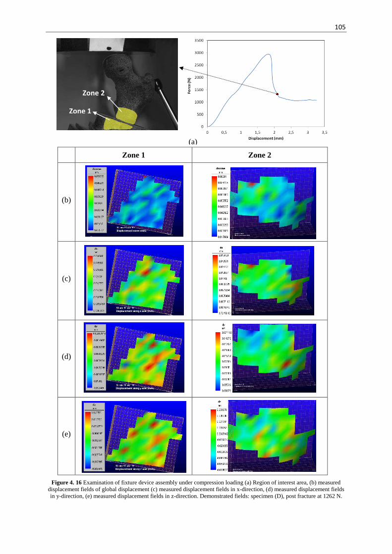
105
(a)
Zone 1 Zone 2
(b)
(c)
(d)
(e)
Figure 4. 16 Examination of fixture device assembly under compression loading (a) Region of interest area, (b) measured displacement fields of global displacement (c) measured displacement fields in x-direction, (d) measured displacement fields in y-direction, (e) measured displacement fields in z-direction. Demonstrated fields: specimen (D), post fracture at 1262 N.
Zone 2
Zone 1

106
4.6. Conclusion
The experimental work will permit to validate the proposed numerical models in chapter
(3). An experimental assembly was designed for compressive tests of human femurs in single
limb stance configuration. The experimental work comprises the testing of eight specimens of
human femur. The novelties of using the 3D optical measurement, advantages of the designed
assembly were introduced. The single limb stance device and the experimental protocols were
successfully validated.
The next chapter will show how experimental results can be predicted by means of the
FE modeling method. The predicted and measured data will be contrasted to each other.

107
Chapter 5
Results and Validation
Abstract
In this chapter, under the assumption of isotropic material properties, we
will first validate the proposed 3D heterogeneous model coupled to quasi brittle
damage law with our experimental results. The numerical results obtained by
the 3D model will be also compared using the experimental results obtained by
3D DIC technique. Its ability of prediction will be evaluated and discussed. In
order to provide a practical and rapid prediction tool, we simplified this model to
a 2D model which is capable in helping the clinical purposes. This model will be
applied into two variants: the first considers damage defined by all strain
components (von Mises equivalent strain). The second, damage was defined by
shear strain only (equivalent shear strain). After its validation, the 2D model will
be applied to study the effect of force direction to represent the consequence of
the daily activities on failure load under both limb stance and sideways fall
configurations. In order to test the capability of our model to predict the
proximal femur failure under sideways fall configuration, the effect of geometry
parameters and density on the fracture force will be evaluated and compared
with the literature. Finally the 2D model will be evaluated by assigning
anisotropic properties for both cortical and trabecular bone for both
configurations.
Résumé
Dans ce chapitre, sous l’hypothèse d’un matériau isotrope, le modèle numérique D proposé couplé à l’endommagement quasi fragile sera validé par les résultats expérimentaux. Une comparaison des résultats de ce modèle avec les
mesures expérimentales obtenus par les mesures de corrélations d’images D sera effectuée et discutée afin de mettre en évidence sa capacité de prédiction.
Afin de fournir un outil pratique et rapide utilisable pour des fins cliniques, le
modèle 3D a été simplifié en 2D. Ce modèle a été appliqué de deux façons
différentes: la première considère l’endommagement comme étant définit par
toutes les composantes de déformation (déformation équivalente de von Mises).
Dans la seconde, l’endommagement a été défini uniquement par la déformation de cisaillement (déformation de cisaillement équivalente). Le modèle 2D de
simulation par EF sera utilisé pour étudier l'effet de la direction de chargement
mécanique pour représenter la conséquence des activités quotidiennes sur la
charge à la rupture sous les deux configurations de chargement: l’appui monopdal et la chute latérale. Afin de tester la capacité de notre modèle à
prédire la rupture du col du fémur dans une configuration de chute, l'effet des
paramètres géométriques et de la densité sur la force à la rupture sera évalué et
comparé avec la littérature. Enfin, le modèle 2D sera évalué en attribuant des
propriétés anisotropes pour l'os cortical et l’os trabéculaire pour les deux configurations.

108
5.1 Introduction
The ability of the proposed FE model to predict hip fracture in human femurs was
demonstrated in chapter (4) by the preliminary comparison with the study of Keyak and
Falkinstein, 2003. We will first validate the proposed three dimensional Finite Element (FE)
model with our experimental results. Secondly, the simplified two dimensional model will be
validated. The capability and the predictive power of the two dimensional model will be
assessed. A parametric study will be performed on the two dimensional FE models.
5.2 Results and validation of the three dimensional finite element simulation
The objective of the 3D FE analysis is to find the distribution of displacements within
the proximal femur and failure forces. As mentioned, the proximal femur model (model A)
was divided into finite elements corresponding to voxels. The voxel elements are of type
(C3D8) with average dimensions of 9.9 × 13.9 × 4.8 mm3 (Table 4.3). The mechanical
properties assigned to each element, as mentioned in chapter (4), are assumed to be isotropic
with heterogeneous Young’s modulus (Equations from 4.1 to 4.4) and a constant Poisson's
ratio of 0.3.
5.2.1 Results and validation of Force-Displacement curve
In Figure 5.1 the force–displacement curves of the tested femurs are shown. All curves
show a linear stage followed by a nonlinear post-fracture behavior caused by damage
initiation. The occurrence of damage is revealed by a sharp drop in force during failure that
was nearly always observed during mechanical testing. The growth of damage can be shorter
or longer depending mainly on bone organ geometry, intrinsic properties, specimen
preparation (fresh frozen, embalmed), aging (decrease of toughness of bone) and the load
testing speed.
The curves presented in Figure 5.1 have been recorded at a very low speed (quasi static
load), thus permitting to identify the breaking modes. Schileo et al. [Schileo et al., 2008]
loaded proximal femurs in single limb stance at high strain rate. The specimens have failed
with a sudden fracture process (sharp decrease of load after reaching the maximum value)
without noticeable post-yielding phase, suggesting the presence of generalized yielding

109
(fracture patterns resembling brittle fracture). A similar failure behavior showing a sudden
structural collapse was reported by Link et al. [Link et al., 2003] and Yang et al. [Yang et al.,
1996].
Figure 5. 1 Measured force displacement curves of human femur specimens.
As shown in Figure 5.1, specimens of the same cadavers (A and B, C and D, E and F)
have nearly a homogeneous linear behavior. Beyond the elastic limit, the bone material is
much less rigid. This is because bone damage accumulation generates microscopic cracks
and/or voids which causes a progressive degradation of material continuity of the material
[Lemaitre and Chaboche, 1990]. The fluctuations on the curves beyond the peaks are due to
the fact that localized contact occurs between the head of the femurs and the piston of the
testing machine.
In the current work, the ultimate force fracturing the femoral neck was taken as the peak
value for the curve. The average ultimate experimental force was 6210 ± 253 N (range: 2010–
8550 N) for single limb stance configurations. These findings are comparable with those
reported in the literature. Indeed, prior investigations of uniaxial quasi static compression tests
performed on eleven right femora conducted by Bessho et al. [Bessho et al., 2007], loaded at
20° in the coronal plane, gave failure loads in the range of 2800-6100 N. Smith et al., [Smith
et al., 1992] reported a range between 4937N and 16148 N, Le bras et al. [Le bras et al., 2006]
found under identical coditions a range of 3100 and 7150 N and Duchemin et al., [Duchemin
et al., 2006] reported an experimental failure load of 9032 ± 3412 N for four human femur
specimens in the frontal plan.
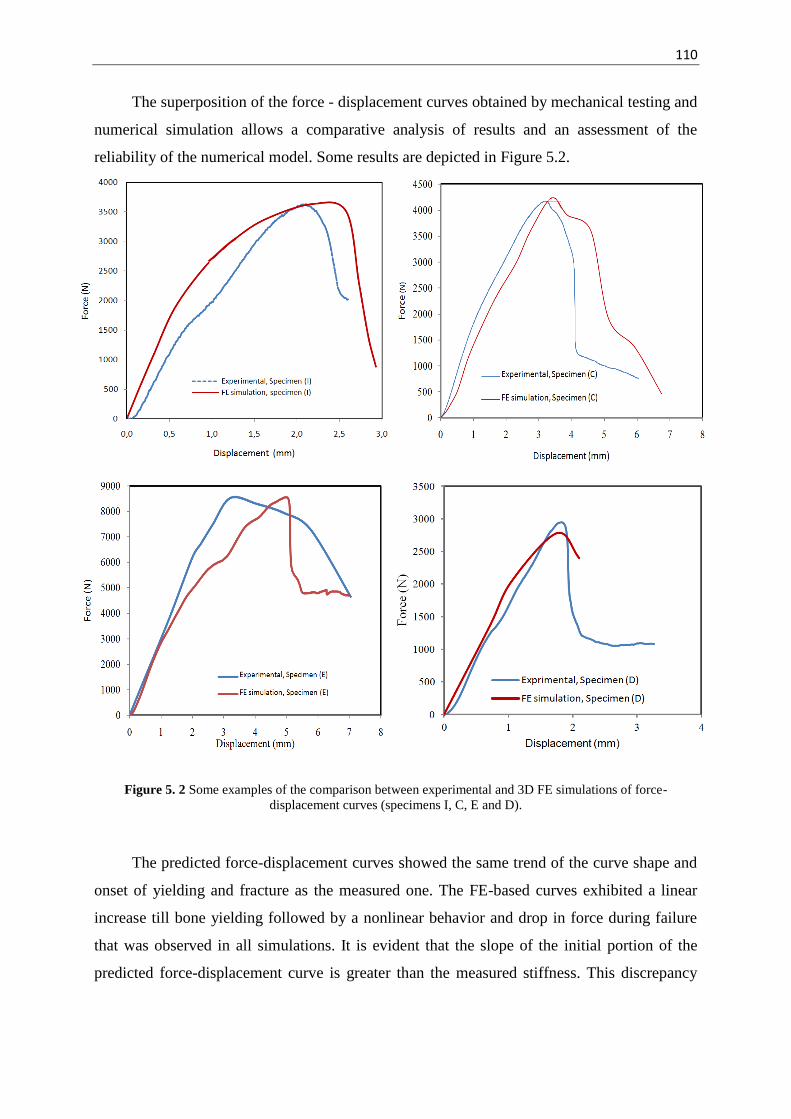
110
The superposition of the force - displacement curves obtained by mechanical testing and
numerical simulation allows a comparative analysis of results and an assessment of the
reliability of the numerical model. Some results are depicted in Figure 5.2.
Figure 5. 2 Some examples of the comparison between experimental and 3D FE simulations of force-displacement curves (specimens I, C, E and D).
The predicted force-displacement curves showed the same trend of the curve shape and
onset of yielding and fracture as the measured one. The FE-based curves exhibited a linear
increase till bone yielding followed by a nonlinear behavior and drop in force during failure
that was observed in all simulations. It is evident that the slope of the initial portion of the
predicted force-displacement curve is greater than the measured stiffness. This discrepancy

111
was explained by the strain-softening behavior of the bone [Keyak, 2001] which is not
implemented in the FE model.
The current FE proximal femur fracture model provided good agreement between
predicted and experimentally measured ultimate force at fracture with a correlation factor for
the entire data set R2 = 0.833 , Figure 5.3.
Figure 5. 3 Current predicted and experimental failure load correlation.
Our fit equation for the failure force under single limb stance conditions can be
expressed in as FExp = 0.912 FNum + 211.2 N, where FExp is the experimental force and FNum is
the predicted value of force. The fit equation from earlier models had less predictive power,
for example FExp = 0.77 FNum + 1150 N [Keyak et al., 2001, Keyak et al., 2005]. Prior
investigations of uniaxial quasi static compression test of human femur were conducted by
Bessho et al. [Bessho et al., 2007]. Using identical conditions under single limb stance of
femur loaded at 15°, Besso et al. found FExp = 0.809FNum + 1592 N [Besso et al., 2007]. Le
Bras et al. [Le Bras et al., 2006] performed the tests under the same conditions and have given
the results of failure forces similar to ours (3000 N and 8000 N) with a correlation between
experimental and numerical data of 0.84, see Figure 5.4.
y = 0,9124x + 211,21
R² = 0,833
1000
2000
3000
4000
5000
6000
7000
8000
9000
1000 2000 3000 4000 5000 6000 7000 8000 9000
Mea
sure
d F
aliu
re Loa
d , N
Prediced Failure load , N
A_D
B_G
C_D
D_G
E_D
F_G
G_G
I_G

112
Figure 5. 4 Predicted and experimental failure load correlation [Le Bras et al., 2006].
Even though, their models arrived at reliable fracture forces, they were unable to predict
the fracture profile as well as the complete force displacement curves. Furthermore, damage
accumulation was not evaluated.
5.2.2 Results and validation of three dimensional fracture pattern
Nonlinear continuum-level voxel models have been used before to study the mechanical
behaviour of the proximal femur beyond the yield point [Cody et al., 1999, Keyak et al.,
2001] up to and beyond maximum fracture stress values. Using the current damage based
model, damage is expected to start in the vicinity of the femur neck. This may be explained by
the thin cortical shell at the neck of the femur (see Figure 5.5a) that diminishes the strength of
the femoral neck [Zysset et al., 1999]. Besides, in this zone trabecular bone is dominant as
shown by the qualitative comparison in Figures 5.5a and 5.5b. The discontinuity due to
damage in the trabecular bone and the smallest section area may lead to stress concentration
and causes finally the failure in the vicinity of the femoral neck (see Figures 5.5 and 5.6).
(a) (b)
Figure 5. 5 Weak areas in femur bone. (a) cross section from CT scanner showing the regions of trabecular bone (left) with FE simulation of the accumulated damage (second left) for a tested sample (specimen I) (b)
BMD image taken from [Langton et al., 2009]. Dashed rectangle refers to neck zone and the solid circles refer to the lack (or cracks) of bone material at the femur shaft.

113
Microdamage in general refers to discrete microcracks, cross-hatched and diffuse
damage. In vivo, microdamage is found in both cortical and trabecular bone. In addition,
microdamage accumulation has been shown to underlie the development of stress fractures
and plays a role in the increased bone fragility associated with aging and osteoporosis. Many
trabeculae in osteoporotic bone are disconnected and whole regions without bone can exist in
the femoral neck zone producing the different types of neck fractures [Thomas et al., 2004].
The single limb stance configuration was able to reproduce the several typical femoral neck
fractures.
Exp
erim
enta
l te
st
FE
sim
ulat
ion
frac
ture
(D
amag
e co
ntou
r)
Figure 5. 6 Fracture sites (upper row) and 3D damage pattern (lower row) for sample (G).
In our sample size, different typical fractures were obtained: 13% cervical, 50%
subcapital, 25% subcapital-cervical and 12% typical facture in the femoral head. Figure 5.7
depicts some of the obtained fracture patterns.
Figure 5. 7 Different obtained fracture patterns of proximal femurs under single limb stance configuration. (Upper row: specimens F, B and I, Lower row: specimens C , E and A).

114
Not only the correlation between numerical and experimental values was similar to
previous studies, also the fracture location site and patterns were alike.
Few investigations have compared the predicted fracture location with that obtained
experimentally and have visibly shown conformity between them. Ota et al. [Ota et al., 1999]
reported on the accuracy of fracture site prediction, but only for one case. Some other studies
compared the experimental fracture site on radiographs with a non-linear model under limb
stance load at 20° [Keyak et al., 2001]. They reported that their models succeeded to
determine the fracture sites for 13 out of 18 specimens under single limb stance configuration.
Recently, Dall'Ara et al. [Dall’Ara et al., 2013] performed a nonlinear CT-based FE model
validation study of human femur loaded in single limb stance and sideways fall configuration.
They tested 36 pairs (17 males, 19 females) with age (76±12) years, range (46–96). In their
single limb stance test, the load was applied also at 20°. They found typical femoral fractures
in most cases (subcapital: 24%, neck: 54%, trochanteric: 13%, atypical in the femoral head:
3%, not clear: 6%). However, Dall’Ara et al’s model succeeded to qualitatively predict in
66% of all cases the failure location and the motion of the femoral head.
A representative example of the experimentally and numerically obtained fracture
pattern is shown in Figure 5.8 for one femur.
Figure 5. 8 Simulated 3D damage contour (left) and fracture sites (right) for a tested specimen (I).
Our results predict slightly different fracture profiles and locations compared to the
experimental results. Such differences may reside in the voxel mesh used for the current
models, the applied boundary conditions and the assigned material properties.

115
5.2.3 Results and validation of three dimensional model using digital image correlation technique
To compare the results of the 3D model to those obtained experimentally using the DIC
method, spatial contour plots of the displacement fields corresponding to different states of
loading were plotted for each femur.
As the surface of the femur is three-dimensional and neither uniform nor plane, the
measurement of the deformation components of the femur surface was not possible. Hence,
our comparison will be based only on the displacement fields gathered from DIC. To achieve
this, the constitutive behavior was divided into three phases: elastic, just before failure and
after failure. For each of these regions, we define different states of loading where we carry
out the comparison of experimental and numerical displacement fields.
These states are identified by the crosshead displacement. The example presented in
Table 5.1 is the specimen B.
Table 5. 1 Post processing treatments on a representative sample (B).
Displacement, mm Load, N Remarks
-0.001 0.00
0.643 991.87 State 1(elastic region)
1.295 1614.47
1.945 2429.39
2.666 3067.29 State 2 (just before failure)
3.333 3560.93 Maximum strength
3.999 1793.86 State 3 (just after failure)
4.666 1436.86
All surface displacement components were recorded. Figure 5.9 shows perspective plots
of the instantaneous displacement taken for the specimen (B), as an example, for the states 1,
2 and 3 defined in Table 5.1.

116
(a)
State 1
State 2
(b)
State 3
State 1
State 2
State 3
(c)
State 1
State 2
State 3
(d) Figure 5. 9 Measured displacement fields in the temporal matching of the compression experiment of a
representative specimen (B).(a) the chosen three states on the force displacements curve, (b) displacement values in y-direction, (c) displacement values in x-direction and (d) displacement values in z-direction.
State 1
State 2
State 3

117
Figure 5.9 shows the obtained displacement fields distribution for the states defined in
Table 5.1.
The vertical displacement component (dy) corresponding to the line of action of the
compressive force is the most relevant one. As shown in Figure 5.9a corresponding to state 3,
the experimental value of the vertical displacement is about 4 mm. DIC measures a maximum
value of 2.7 mm. Thus, there is a discrepancy of 50%. This deviation is mainly due to the
following reasons:
The crumbling and ensuing damage of the femoral head caused by the head
plate. This translates into a loss of local stiffness which can be easily identified
on the curve (such as between 1.3 and 1.8 mm on the curve, Figure 5.9a).
The maximum experimental displacement of 4 mm is the one of the head plate
and represents the displacement of the contact point of that plate with the femur
tip. The selection of the ROI for DIC was dictated by the need to observe
identical zones throughout the entire test. Hence, areas directly in contact with
the head plate were not tracked.
Throughout a compression (or tension) test, the local deformation varies within
the volume. Heterogeneity causes displacement and deformation to deviate more
from the values at the head plate the greater the distance from that point.
The displacements dx and dz are not zero as shown on Figure 5.9c and 5.9d. Those
components are measured when the femoral head is damaged and bent or broken.
The resultant displacement vectors comparisons are presented in Figures 5.10a, 5.10b
and 5.10c. The displacement is characterized by a gradual variation from the point of load
application (red arrows) about 1.6 mm (Fig 5.10b) to the lowest values about in the trochanter
region (blue values). The spatial variation of displacement comparison shows a remarkable
consistency between the numerical and experimental recordings.
The results presented in Figures 5.9 and 5.10 show that the higher part of the proximal
femur, i.e. the head and subcapital zone in Figure 5.9b (stat 3) were displaced by a value
ranging from 1.01 mm to 2.01 mm. The lower part of the proximal femur, i.e. the neck and
trochanter, were displaced by 0.02 mm to 0.27 mm. Similarly, at the femoral neck, if we take

118
Figure 5. 10 Comparison between the predicted displacements (right), mm and measured displacement fields, mm by DIC method (left) for specimen B. (a) elastic region at 991.87 N, (b) just before failure at 3067.29 N
and (c) just after failure at 1793.86 N.
(a)
(b)
(c)

119
average differences between the upper and lower parts of the proximal femur are 0.47 mm
and 0.18 mm respectively. With such a relatively high interface variation of the response, it
can be suggested that the failure may take place by shearing at the neck zone.
It is obvious that the measurement of the displacement with the DIC method is more
suitable than the strain gauges. As they permit to acquire only local point measurements while
the DIC method gives the local and global fields distribution.
5.3 Results and validation of the two dimensional finite element model
The clinical implementation of 3D CT/FE methods is still limited due to the
requirement of expensive computer hardware to achieve solutions of 3D FE models within a
clinically acceptable time, as well as, the need for robust 3D segmentation and meshing
techniques [Aspray et al., 2009]. Segmentation, meshing and FE analysis of a 2D geometry
can be accomplished fast and is potentially more robust than 3D CT/FE [Langton et al.,
2009]. DXA scanners are becoming more widely available and they play an increasingly
important role in clinical practice [Testi et al., 1999]. It is currently the clinical standard for
assessing osteoporotic fracture risk but is not a reliable predictor of fracture [Aspray et al.,
2009]. In several studies, the status of the proximal femur has been examined in vivo by
DXA.
In order to provide a practical and rapid tool, we simplified our 3D model to a 2D model
which is capable in helping the clinical purposes. This 2D model, preliminarily validated in
chapter (3), models test-I and test-II , will be validated using the 2D-DIC measuring technique
and finally its capability will be evaluated and discussed in the following subsections.
5.3.1 Results and validation of single limb stance model
In a 3D-DIC technique, color-coded displacement values represent at high spatial
resolution the topography of the moving surface when subjecting the femur to a load.
Notwithstanding the fact that the femur surfaces are not flat, the 2D-DIC visualization
technique is capable of representing an appropriate and realistic mapping of the fracture
pattern.
Contrary to the 2D-DIC technique, the spatial resolution of the 3D-DIC technique does
not allow locating the precise spot of fracture initiation. Hence, though the comparison is only
qualitative in nature, but not quantitative, the reliability of the 2D-DIC technique can be

120
corroborated and additionally lend support to the hypothesis that the out-of-plane deformation
component is less relevant for the deformation process and fracture profiles.
The local displacement and strain fields at the femur surface were evaluated by utilizing
7D software in 2D based on DIC technique. In the 2D-DIC procedure, images were taken at
each time increment. During image acquisition, the corresponding displacement and the
applied load were also recorded. Figure 5.11a presents the force-displacement response for a
representative specimen along with DIC data presented in Figure 5.11b. The fields of the
maximum shear, maximum/minimum principal strains are presented for three chosen states:
elastic loading (state 1), before failure (state 2) and post failure (state 3). The results indicate
distinctly different patterns of strain development for single limb stance configuration. The
maximum shear was found at the proximal femur with a distinct anterior concentration of
both maximum shear and minimum principal strains. This may be explained by the particular
density distribution at neck region supcabital zone. This result was also observed by other
investigations. Cristofolini et al. [Cristofolini et al., 2007] investigated, in vitro, the
occurrence of spontaneous fractures of proximal human femur. Surface strains were recorded
by using strain gauges. They found that the most common fracture initiation site was the
subcapital region (80% of their 10 cadaveric femur specimens). This is not surprising since
the boundary condition is essentially a constant axial displacement across the longitudinal y-
component where the shear takes the place. The reduced bone mass at the femur neck due to
the concentration of trabecular bone (as presented in Figure 5.5) and a high bone loss at this
site [Chevelley et al., 1991] suggest the initiation of fracture in this area. This lack of strength
was also elucidated in the current work as 75% occurred in the neck femur fracture of
subcapital and subcapital-cervical zone, as shown in Figure 5.7. The plots are more sensitive
to subtle differences of maximum shear distributions at trochanter and diaphyseal regions
which are also characterized by general homogenization of maximum and minimum strains
(Figure 5.11b, state 3) produced by the applied load.

121
(b)
Figure 5. 11 Shear and principal strain distribution for the two dimensional measurement areas of a proximal femur (specimen B). (a) the chosen three states on the force displacements curve (b) corresponding shear and
principal strain distributions (maximum and minimum) contours.
The measured strain values were ranged from 0.35% to 0.56%. In many other
investigations, when surface strains of femur are of interest, a larger number of strain gauges
were bonded on the femur surface [Cristofolini et al., 2007, Taddei et al., 2006, Viceconti et
Ma
xim
um
sh
ea
r M
axim
um
princip
al str
ain
State 3 State 2
Min
imum
prin
cip
al str
ain
State 1 State 2 State 3
State 1
State 3 State 2 State 1
State 1
State 2
State 3
(a)

122
al., 1998, Yosibash et al., 2007]. In these works, the local strains were reported as 0.33% (see
Figure 5.12) [Viceconti et al., 1998], between 0.1% to 1.0 % [Taddei et al., 2006] and 0.12%
to 0.16% [Taddei et al., 2007].
Figure 5. 12 Axial strains measured in vitro using strain gauges along the femoral shaft. Experimental data points are denoted by ‘x’ [Viceconti et al., 1998].
The distribution of deformations along the femur shaft for a representative femur
specimen is presented in Figure 5.13. The vertical deformation ( ) and horizontal
deformation ( ) are presented for two states: at maximum strength and just after failure. In
terms of values, the measured deformations corresponding to these two states are between -
0.55% and +0.33%. The extrema of these values occur in both compression and tension sides.
By comparing these findings with those using strain gauges along the femoral shaft
mentioned in the experimental work of Viceconti et al. [Viceconti et al., 1998]. A values of
-33% and +0.32% were found corresponding to the compression and tension sides.
Our goal in the current work is to use the DIC measurements for a qualitative
comparison. The comparison between our deformation measurements obtained with the DIC
with those reported in the literature [Taddei et al., 2006, Viceconti et al., 1998, Taddei et al.,
2007] suggest that our DIC measurements can be used for quantitative validation.

123
at maximum strength just after failure Deformation
at maximum strength just after failure
Deformation Figure 5. 13 Axial strains measured in vitro using DIC technique along the femoral
shaft (specimen B).
5.3.1.1 Results and validation of two dimensional fracture pattern
Damage in bone could be caused by shear failure of the organic matrix [Kotha and
Guzelsu, 2003]. The single limb stance configuration has been shown in previous studies to
produce maximum shear stresses in the femoral neck region in a manner consistent with
clinical subcapital fractures [Smith et al., 1992, Cotton et al., 1994] similar to the predicted
ones.
Stress-strain criteria are the most widely applied criteria for strength evaluation of
materials. Quasi brittle behavior could be accepted to behave linearly elastic before reaching
its proper threshold level of stress. In the elastic range, the stress criterion is equivalent to the
strain criterion. The strain equivalent criterion is based on a limiting energy of distortion, i.e.
energy associated with shear strains. This criterion has succeeded to give good validated

124
results and is widely used for estimating the proximal femoral fracture load and assessing hip
fracture risk [Ford et al., 1996, Keyak et al., 1998, Lotz et al., 1991a].
Trabeculae in the subcapital region collapsed under the applied load. The damage
distribution sequences of the presented specimens F and A given in Figure 5.14 (two left
columns) indicate that damage accumulation occurred during the loading which ultimately
formed a high strain concentration region in the form of shear band. In the current study, the
2D models were applied into two variants:
The first considers damage defined by all strain components (von Mises
equivalent strain) and for which results are presented in the first column of
Figure 5.14.
The second, damage was defined by shear strain only (equivalent shear strain)
and for which results are shown in the second column of Figure 5.14.
The fracture patterns obtained with the 2D models were compared with the maximal
shear strain, measured using 2D digital image correlation, just before the femur specimens
failure and the experimentally obtained fracture patterns in the two right columns of Figure
5.14.
It is well known that bone resistance to shear is weaker than in tension and compression.
The analysis revealed that equivalent strain was concentrated in the inferior cortex of the
subcapital region. Microcracks have been observed in cortical [Morgan et al., 2005] and
trabecular [Wachtel and Keaveny, 1997] tissue following compressive overloads and have
been suggested to result from local shear stresses.
The simulation presented in Figure 5.14 (second column) was applied with considering
only the effect of shear strain components under axial compression. The results show that the
damage computation incorporates exclusively the shear strain components. This can be
explained by behavior of bone under excessive mechanical load which is characterized by
diffuse microcracking and localizes in relatively narrow zone, referred to fracture process
zone [Vashishth et al., 2000].
This zone was the origin of a major crack that resulted in a catastrophic failure. In
normal gait, the greatest stresses occur in the subcapital and mid-femoral neck regions. Within
these regions, maximum compressive and shear stresses occur inferiorly and tensile stresses
of small magnitude occur superiorly [Lotz et al., 1995].

125
Numerical Experimental
damage defined by
all strain components
damage defined by shear strain only
Post testing y-
displacement due to shear
Experimental test
specimen (F)
specimen (A)
Figure 5. 14 Prediction of failure location. Damage defined by all equivalent strain components (first column). Damage defined by shear stain only (second column). Dashed circles highlight the failure location from the
experiments and are reported in solid on the models. The arrows indicate the fracture site. Solid circles at the diaphysis of the presented specimen (F) refers to a damaged zone that may be explained by a lack of mass
density in this specimen.
The failure due to equivalent shear strain was studied in the current work under single
limb stance configuration by using 2D FE models. The obtained damage contours are
compared with experimental failure due to shear. Figure 5.15 present some examples of this
comparison.
The predicted and actual fracture locations were consistent for all femora. The current
FE proximal femur fracture model provided excellent agreement between predicted and
experimentally (DIC) displacement values and distribution.

126
Numerical results of the 2D models Experimental results Specimen B :
Specimen C :
Specimen D :
Specimen G :
Figure 5. 15 FE and experimental Fracture patterns under single limb stance configuration.
As shown in the comparisons presented in Figure 5.16, the subcapital fracture resulted
under limb configuration. The region of the greatest principal displacement of the femur head
(1.47 mm to 2.3 mm) is the predicted fracture site at subcapital zone.

127
(a) (b)
Figure 5. 16 Displacement fields (mm) just before failure for specimen (B) measured by: (a) 2D-FE model (b) 2D-DIC method.
The formation of a shear band which ultimately causes the subcapital fracture is the
consequence of local material response. It depends mainly on the local apparent trabecular
bone density [Ford and Keaveny, 1996]. At the elastic deformation phase (prior to yielding),
the external load causes local homogeneous strains within the femur neck. After damage
initiation, strain gradient instability occurs due to the difference of resistance of the trabecular
bone and generates the shear band.
Our findings suggest that when damage taken into consideration, the predicted fracture
sites are more precised. Furthermore, the predicted fracture forces were less when defining
damage only by shear components suggesting that shear failure plays a large role in trabecular
bone fracture [Ford and Keaveny, 1996]. The proposed damage law defined by the von Mises
equivalent strain suggests that yielding and cracking begins when the elastic energy of
distortion (also known as the shear energy) reaches a critical values of applied strains [Hill,
1950]. The suggested equivalent strain in the FE damage model can be considered as an
adequate variable to capture the damaging process within bone since the equivalent strain is
expressed in function of the deviatoric strain tensor which captures the shearing component of
the applied strain.

128
5.3.1.2 Comparison between the predicted two dimensional model and experimental force displacement curves for single limb stance
Results from 2D FE analyses have been previously validated with those obtained with
a 3D FE analysis of CT data. Testi et al. [Testi et al., 1999] found good agreement between
the results of a 2D FE model with a DXA image to 3D FE model, and also validated the
results in-vitro. Based on 2D structural geometry derived from DXA, Mourtada et al.
[Mourtada et al., 1996] used the BMD data to propose a 3D model from a 2D DXA data.
Recently, Buijs and Dragomir-Daescu [Buijs and Dragomir-Daescu, 2011] used a 2D FE
model derived from CT scans of human femur. The strain distributions were identified from
recorded high speed video of the fracture procedure and were validated against the FE results.
While an acceptable agreement was found, our current approach proposes a 2D FE
based DXA projection from the BMD data. This model takes in consideration the material
properties for both cortical and trabecular tissues with significant accuracy. See Figure 5.17.
Figure 5. 17 Correlation between experimental and predicted proximal femur fracture under single limb stance configuration.
As shown in Figure 5.17 there is a significant linear correlation between the predicted
fracture load FE analysis and the measured values (r2 = 0.867). By applying the calibration
coefficient of 3, reasonable accuracy was obtained as shown in Figure 5.18.
y = 3,0096x R² = 0,8675
0
1000
2000
3000
4000
5000
6000
7000
8000
9000
10000
0 500 1000 1500 2000 2500 3000 3500
Exp
erim
enta
l fra
ctur
re fo
rce
, N
Predicted fracture force (FE_2D), N

129
Figure 5. 18 Experimental and equivalent 2D force displacement curves.
The results showed that our proposed coupled approach results in a good correlation
between 2D FE force displacement and measured curves. Even though the isotropic scalar
damage variable which is implemented in the proposed model achieves a good agreement
with the experimental obtained, the assumption of anisotropic damage may give more close
results.
5.3.1.3 Effect of force direction on femoral fracture load in single limb stance
The head of the femur is attached to the femoral shaft by the femoral neck, which varies
in length depending on human body anatomy. The cervical-diaphyseal angle varies around
0
500
1000
1500
2000
2500
3000
3500
0 1 2 3 4 5
Fo
rce
, N
Displacement, mm
Experimental
2D FE, Specimen (A)
0
500
1000
1500
2000
2500
3000
3500
0 1 2 3 4 5 6
Fo
rce
, N
Displacement, mm
Experimental
2D FE, Specimen (C)
0
1000
2000
3000
4000
5000
6000
7000
8000
0 1 2 3 4 5 6 7 8
Fo
rce
, N
Displacement, mm
Experimental
2D FE, Specimen (E)
0
1000
2000
3000
4000
5000
6000
7000
8000
9000
10000
0 1 2 3 4 5 6 7 8 9 10
Fo
rce
, N
Displacement, mm
Experimental
2D FE, Specimen (F)

130
125±5° in the normal adult. During the daily activities, the hip transmits a resultant contact
force (F) through the acetabulum to the head of femur [Bergmann et al., 2001].
According to this anatomy the angle excerted by hip on the head femur varies. In
addition, other normal activities, such as: slow walking, normal walking, fast walking,
upstairs, downstairs, standing up, sitting down, standing on 2-1-2 legs and bending of the
knee can vary the inclination of the resultant hip force on the head of the femur (see Figure
5.19).
Figure 5. 19 Contact force vector F (Frontal plan) during nine activities [Bergmann et al., 2001].
If we consider the 3° offset of the femoral shaft axis from the frontal plane [Hollister et
al., 1993 Sermon et al., 2012], the inclination of the contact force from the frontal plane varies
from 10° to 25° depending on the type of activity (see Table 5.2). These angles correspond to
daily activities and are based on the study performed by Bergmann et al. [Bergmann et al.,
2001].
Table 5. 2 Hip force angles versus the daily activities.
Hip loading angle Daily activities α ≤ 10° Standing on 2-1-2 legs
10° < α ≤15° Downstairs, fast walking, slow walking 15°< α ≤25° Normal walking, upstairs, Sitting down, standing up, knee bend
In the current work, model (C) was developed to study the effect of force direction to
represent the consequence of the daily activities on failure load under limb stance
configuration, Figure 5.20. Five angles (α = 5°,10°,15°,20° and 25°) of the load vectors on
proximal femur represent the various activities.
Force directions were referenced to the 2D plane. To evaluate the effect of the various
loading conditions on the head femur fracture, the applied force in each loading condition is
compared with the load at 20° that is considered as reference.
F F F

131
Figure 5. 20 Force directions for single limb stance loading condition (Frontal plane).
The force displacement curves are superposed to determine the force directions
achieving the lowest fracture load under single limb stance, Figure 5.21.
Figure 5. 21 Force displacement curves at different load angles: 5°,10°,15°, 20°, 25° (specimen I).
It is evident that the highest fracture forces occur at angles between 15° and 25°
corresponding to normal walking, sitting and walking upstairs. So the femurs are more
intensely resistant in these conditions (angles of 15° to 25°). The force acting on the femoral

132
head can be split into two different actions. The first one is the vertical component, generating
a bending moment on the head whereas the second (horizontal) component exerts a
compressive force on the head. When the angle increases, the vertical component will
decrease and the moment value on the proximal head will decrease.
Bergmann et al. [Bergmann et al., 2001] perform an investigation about the hip joint
loads during the nine daily activities. The objective of their study was to provide a database of
the measurements of hip contact forces of human proximal femur during the most frequent
activities of daily life. In their analysis, it was found that the measured axial component of the
3D resultant force, Fz , was close to the total resultant force as shown in Figure 5.22. This
suggests that this component has the major effect of proximal femur failure. In the current
study the vertical component, Fz , as well as the horizontal component, Fx ,were taken into
consideration for calculating the failure forces of proximal femur.
Figure 5. 22 Contact force F during nine activities [Bergmann et al., 2001].
The current investigation provides information on the forces applied by hip on the head
femur by the frequent daily activities angle.

133
However, the obtained results did not convey a significant influence of the angle on the
predicted fracture pattern, Figure 5.23. As a rule, the most of the resulted fracture types
remains subcapital fracture. Subcapital fractures are the most common types of spontaneous
fractures [Cotton et al., 1994].
(5°) (10°) (15°)
( 20°) (25°)
Figure 5. 23 Fracture pattern during different applied load directions under single limb stance configuration (specimen A).
In all specimens used by Bessho et al. [Bessho et al., 2007] under identical conditions
(limb stance, 20°), fractures occurs at the subcapital region. This was explained by the
collapse of trabeculae in the subcapital region. In their FE analysis it was found that the solid
and shell elements subjected to compressive failure were at the subcapital region. This
contributed to confirming the accuracy of the current simulation model.
5.3.2 Sideways fall configuration results
5.3.2.1 Resulted two dimensional fracture patterns under sideways fall configuration.
In order to evaluate the risk of fracture as well as its type, if the tested femur is exposed
to a sideways fall instead of single limb stance load, the 2D FE models were loaded until
fracture under sideway fall configuration. The applied loads and boundary conditions were
mentioned in chapter 3.

134
The resulting damage patterns and fracture types of some specimens are presented in
Figure 5.24.
Specimen A Specimen B
Specimen C Specimen D
Specimen F Specimen G
Figure 5. 24 Facture location and fracture pattern for side way fall configuration.
As shown in Figure 5.24, fracture starts at the same area (the weakest zone). The
predicted fracture types appear to be in the basiservical zone in sideways falls as shown in
Figure 5.24 for specimens A, B, C, D, F and G. In the specemines A and B, the highest
damage accumulation due to a fall occurs in the cortex of the femoral neck and large
compressive stresses develop in the superior region (Figure 5.24). Mayhew et al. [Mayhew et
al., 2005] reported that human proximal femurs have thinner superior than inferior cortices at
the mid femoral neck region. As shown in our results in specimens A and C, it was remraked
that the damage appears in the inferior cortex. This is evident as during the sideways fall on
the greater trochanter, the maximal compressive strain occurs at the superior femoral neck

135
[Lotz et al., 1995, Pinilla et al., 1996] with maximal tensile strain in the inferior cortex [de
Bakker et al., 2009].
Under axial compression load testing under sideways fall configuration, femurs
commonly fractured at the thin superior cortex [de Bakker et al., 2009]. In the current work,
the predicted fractures were found mainly at the femoral neck as the basicervical type in
specimens A, B and C or subcapital fracture in D, F and G. Very recently, the trabecular
bone micro architecture of the femoral neck was studied in elderly women both with and
without a hip fracture. The fractured cases had lower bone volume fraction, lower
connectivity density and higher trabecular separation. Particularly, the superolateral region of
the neck displayed substantial trabecular microarchitectural weakness in the elderly women
who had sustained a femoral neck fracture [Milovanovic et al., 2012].
5.3.2.2 Effect of load direction angle on the damage of human neck femoral under sideways fall configuration
Two-dimensional FE model (model C) of cadaveric femurs was developed to study the
effect of load direction on the damage of femoral neck. For the fall configuration, the force
was applied to the femoral head at an angle (α) with the y-direction, Figure 5.25. The surface
of the greater trochanter opposite the load was restrained in the direction of the applied load,
but is free to slide horizontally. The angle (α) represents the angle between the shaft and the
ground.
Figure 5. 25 Force directions for the sideways fall configuration.
In most sideways fall configurations investigations, a 10° angle (α) with the horizontal
was adopted. The angle (α=10°) represents the load at 0° is the reference case [Bouxsein et
al.,1995] which is used in most sideways fall configuration experimental tests.
X
Y

136
In this investigation, under sideways fall configurations, the femurs were subjected to
different load directions through changing the shaft angle with the horizontal from 0 to 15°.
This range of angles was taken in cw (clock wise) and ccw (counter clock wise) direction (see
Figure 5.26) in order to investigate the effect of load direction on proximal failure load. If
successfully validated, such methods could be clinically applied to predict patient bone
strength using simpler and less costly radiographs.
Figure 5. 26 An example of the predicted different damage patterns at different load directions (at the same increment state), specimen C.
At the same displacement, during a sideways fall on the greater trochanter, the greatest
compressive stresses occur in the superior femoral neck while the smaller tensile stresses
occur in the inferior region [de Baker et al., 2004].
(a) α =0°
(b) α =-5°
-α (cw)
(c) α =-10°
(d) α =-15°
Damage due to compressive stresses in superior femoral neck
(e) α =+5°
(f) α =+10°
(g) α =+15°
+α (ccw)

137
Clearly, a strong correlation between fracture load and load direction was found (R2 =
0.815). The most critical cases are ‘c’ and ‘g’ which correspond to α=-10° and
α= -15° respectively as shown in a representative sample (Figures 5.27a and 5.27b).
(a) (b)
Figure 5. 27 Effect of loading direction on predicted fracture load under sideways fall conditions (specimen ‘D’, age =91, Male, left femur). (a) Equivalent 2D Force-displacement curves at different loading angles
(b) impact of loading direction on fracture load.
It can be seen from Figure 5.26 that the amount of damage accumulation is also affected
by the loading angle. As these damage patterns resulted from stress fracture, they can
represent thus the resulted type of fracture pattern [Voo et al., 2004]. The obtained damage
profiles represent typical fractures types: cervical fracture propagating parallel to the neck in
the cases ‘b’, ‘c’ and ‘g’, showing two crack initiation sites laterally, which indicate the
fracture risk area and initiation of subcapital cracks in cases ‘c’ and ‘g’. Finally a cervical
fracture, propagating also parallel to the neck, but including a secondary subcapital crack on
the medial side results in case ‘d’.
However, it is hardly feasible to determine all parameters which influence femur
fracture. Other factors than scrutinized here might also affect the structural capacity of the
femur, and many studies on bone strength of the proximal femur have been reported. For
example, the study of Lotz and Hayes [Lotz et al., 1990] investigate the correlation between
fracture load of human femur and its density. They reported the loads and energies needed to
cause a proximal femur fracture. Courtney et al. [Courtney et al., 1995] studied the effect of
age and loading rate on the femur failure. They compared the loads at fracture of the proximal
femur from the cadavers of older and younger individuals. They reported a 20% increase in

138
failure load due to the high displacement rate [Courtney et al., 1994]. Keyak et al. [Keyak et
al., 2001] investigated the influence of loading direction on the fracture load of the elderly
proximal femur. Ford et al. [Ford et al., 1996] also reported the structural capacity of the
proximal femur in four loading configurations that represent a range of possible falls on the
greater trochanter. Pinilla et al. [Pinilla et al., 1996] studied the influence of changes in
loading angle, under sideways fall position, on the failure load of the proximal femur ex vivo
and on the fracture pattern. They assigned in their investigation three distinct loading angles
0°, 15° and 30° to simulate three fall positions: fall on the hip rolled slightly forward (0°
position), to side (15°) or rolling slightly backwards (30°). The 15° loading configuration was
identical to that used by Courtney et al. [Courtney et al., 1995]. The angle of the femoral shaft
with respect to the horizontal (defined as femoral shaft angle) was 10°. Their results showed
that a slight variation in the fall-related loading angle significantly reduces the failure load of
the proximal femur. The femurs tested at 30° failed at a 24% lower load than the ones tested
at 0° i.e. from 4000N at 0° to 3000N at 30°.
However, all these studies have highlighted that the loading direction influences the
generation of a proximal femur fracture. The limitation of these studies is that they used
subjects affected by osteoporosis. Furthermore, damage was not evaluated. In the current
thesis, both were taken into consideration through using the damage as a coupling approach
and the heterogeneous mesh.
The fracture patterns revealed by our model in sideways fall configuration were not
significantly dissimilar suggesting that the load direction has not a significant effect on the
fracture pattern at the used range of load directions (α=0° ± 15°). Our conclusion is confirmed
by Pinilla et al. [Pinilla et al., 1996] who discussed also whether the fracture location is
affected by loading direction. They found no significant difference in fracture patterns among
the three groups.
The damaged zone due to the accumulation of equivalent strain was qualitatively
compared with the an elastic equivalent strain field obtained with the 2D FEA model of
representative proximal femur image obtained from high speed video recordings using digital
image correlation from [Buijs and Dragomir-Daescu, 2011]. This qualitative example is
presented in Figure 5.28.

139
Figure 5. 28 A Qualitative comparison of damaged areas in sideways fall configuration (a) 2D damage accumulation (current FE model) (b) Elastic equivalent strain distributions in a validated 2D-FE model of
proximal femur [Buijs and Dragomir-Daescu, 2011].
Our results suggest that the damage occurs in areas which experience maximum strains.
Previous investigations have concluded that neck femur fractures are typically initiated by a
failure in the superior side of the femoral neck, followed by a failure in the inferior aspect of
the femoral neck [de Baker et al., 2009, Lotz et al., 1995]. This can be explained by several
factors:
The femurs with a longer moment arm are exposed to higher forces applied to
the hip [Wang et al., 2009].
A fall onto the greater trochanter may also generate an axial force along the
femoral neck, resulting in fracture due to the impact force.
The lower extremity rotates externally during a fall on the femoral neck which
impinges against the posterior acetabular rim. The acetabular rim then acts like
a fulcrum to concentrate the stress experienced by that region upon impact
[Koval & Zuckerman, 1994].
5.3.2.1 Effect of geometric parameters and density on the fracture force of human proximal femur under sideways fall configuration
There is indisputable evidence that BMD as measured by DXA, particularly at the
proximal femur, is a strong predictor of hip fracture [Cummings et al., 1993]. However,
considerable overlap exists in BMD values between subjects with and without hip fractures,
suggesting that the geometry the proximal femur may contribute to femoral neck strength
[Bergot et al., 2002].
(a) (b)
Accumulated damage
Maximum elastic equivalent strain

140
In this study of proximal fracture risk evaluation from hip DXA scans, our objective
was to test the potential of our proposed coupled damage approach to predict the proximal
femur under sideways fall configuration. Using the heterogeneous isotropic model, model C,
the effect of femoral neck width, femoral neck axis, cervical diaphyseal angle and density on
the strength of the proximal femur will be evaluated and compared with those obtained in
literature.
Figure 5.29 compiles the predicted femoral fracture load under sideways fall
configuration correlated with femur geometry and density. The effect of femoral neck width
(Figure 5.29a) and the femoral neck axis length (Figure 5.29b) support the results previously
reported in hip fracture patients [Alonso et al., 2000, Gnudi et al., 1999, Karlsson et al., 1996].
Figure 5. 29 Effect of femur geometry and density on the femur fracture load under sideways fall configuration. (d) (e)
(c)
(a) (b)

141
Hip axis length (Figure 5.29b) and neck shaft angle (Figure 5.29c) both contribute to
the moment arm of the hip and both have been independently shown to influence hip fracture
[Leslie et al., 2009, Patron et al., 2006].
However, this effect cannot be considered as universally valid in the current
investigation due to the small sample size and the absence of experimental validation tests.
Alternatively, some specimens have less resistance even though they are characterized by
higher neck density.
The results assembled in Figures (5.29d and 5.29e) imply the fact that the failure load
is proportional to the femoral neck density. Hence, it can be inferred that the model using the
isotropic behavior coupled to damage can give reasonable results.
5.4 Anisotropic finite element modeling results for single limb stance and sideways fall configurations
In the current work, 2D heterogeneous models coupled to quasi brittle isotropic
damage law were evaluated by assigning anisotropic properties for both cortical and
trabecular bone (Model B). The fracture of the femoral head and stiffness in both single limb
stance and sideways fall configurations were evaluated.
Under single limb stance configuration, the correlation between the predicted failure
load and the predicted stiffness was moderate (R2=0.51), Figure 5.30a. In contrast, fair
agreement (R2=0.75) was obtained for the correlation between the predicted stiffness and
BMD of the femoral neck, Figure 5.30b.
Figure 5. 30 Correlations under single limb stance configuration. (a) between 2D FE stiffness and predicted failure loads (b) between femoral neck density and predicted 2D FE stiffness.
R² = 0,7458
0
500
1000
1500
2000
2500
3000
3500
0,20 0,40 0,60 0,80 1,00
Pre
dic
ted
Stif
nes
s, N
/mm
2
BMD of Neck, g/cm2
(a) (b)
R² = 0,5058
0
1000
2000
3000
4000
5000
6000
7000
8000
9000
1000 1500 2000 2500 3000 3500
Pre
dic
ted
For
ce,
N
2D FE stiffness, N/mm

142
Although most studies adopted the isotropic assignment in their simulations, bone was
occasionally interpreted as being orthotropic [Peng et al., 2006, Taylor et al., 2002, Wirtz et
al., 2003]. So far, the impact of using a model with orthotropic material property assignment
compared to an isotropic model is still a matter of dispute [Peng et al., 2006].
For sideways fall configuration, the correlation between the predicted stiffness and
predicted force was relatively strong (R2 = 0.86) for our sample size specimens. The findings
were compared with a recently validated 2D model [Buijs and Dragomir-Daescu, 2011], see
Figures 5.31a and 5.31b.
Figure 5. 31 Correlation between stiffness and failure loads under sideways fall configuration. (a) predicted fracture load versus predicted stiffness obtained by current FE model, (b) Measured failure load versus predicted FE stiffness obtained by 2D FE model proposed by Buijs and Dragomir-Daescu, [Buijs and Dragomir-Daescu,
2011].
Our results show that the 2D FE models yield substantially accurate predictions of the
femoral stiffness and ultimate proximal femur strength. The predicted stiffness is correlated
with the neck femoral density by a not very significant correlation was found (R2=0.53), see
Figure 5.32a.
In the current study, we have investigated the relationships occurring between BMD of
the femoral neck, 2D bone structure parameters calculated from DXA images and predicted
bone 2D stiffness. It was reported that BMD can be used as a predictor of bone strength in
cortical bone, i.e., in the femoral shaft.
However, when trabecular bone is present in the specimen (as in the femoral neck),
BMD is of limited value in predicting bone strength, showing only a weak correlation with
stiffness. This has earlier been stressed by Buijs and Dragomir-Daescu, Figure 5.32. Their
data set shows a weak correlation (R2= 0.48).
(a) (b)
R² = 0,8547
0
1000
2000
3000
4000
5000
6000
7000
8000
0 500 1000 1500 2000 2500 3000
Pre
dic
ted
For
ce,
N
2D FE Stiffness, N/mm

143
Figure 5. 32 Correlation between femur neck density and femur stiffness under sideways fall configuration. (a) Current 2D FE model (b) Experimentally obtained stiffness versus BMD [Buijs and Dragomir-Daescu, 2011].
5.5 Conclusion
Our aim in this chapter was to validate the developed 3D FE models as well as the
simplified 2D models using eight experimentally tested femurs. In this chapter we validated
the proposed 2D and 3D FE models describing the progressive proximal femur fracture under
single stance load and sideways fall configurations in the quasi-static regime.
The adopted equivalent shear strain in the FE damage model can be considered as a
reliable variable able to simulate the fracture process till complete fracture.
The local and global surface deformation measurements of the proximal femur head was
carried out by DIC method.
Our 3D results succeeded to predict the complete force displacement curves as well as
the location of the fracture initiation. The total fracture patterns were slightly different from
those obtained experimentally suggesting that the used voxel mesh method may not lead to a
better prediction of the 3D fracture shape. Although CT based 3D FE analysis can give
reliable predictive information on the complex proximal femur, a 2D FE model from DXA
images may be sufficient for clinical purposes. The proposed simplified 2D model was
preliminarily validated by another previously published model under identical boundary
conditions. The obtained 2D force displacement curves were qualitatively compared with
results from experiments and from the literature. Our model achieves a qualitatively good
(a) (b)
R² = 0,533
y = 3554x - 1161
0
500
1000
1500
2000
2500
3000
0,00 0,20 0,40 0,60 0,80 1,00
2D
FE
sti
ffn
ess
, N
/mm
BMD of Neck, g/cm2

144
match. Contrary to the proposed 3D model, the 2D model succeeded to predict the fracture
location as well as total fracture profile by using voxel method.
The Femoral neck axis length, neck width, and neck-shaft angle were measured on
radiographs of ten proximal femora. Bone mineral density (BMD) was measured using dual
energy X-ray absorptiometry (DXA) for the region of interest. The strength of the femur was
determined by a mechanical test simulating a single limb stance and the fracture type
(subcapitcal, cervical or trochanteric) was subsequently determined and discussed. Among
our samples, 13% cervical, 50% subcapital, 25% subcapital-cervical and 12% atypical facture
in the femoral head were observed. Under sideways fall configuration, DXA total density was
more strongly correlated with femoral strength (R2= 0.76). A significant correlation was
observed between femoral strength and neck width (R2 = 0.65). Weak correlations were
observed between fracture force and femoral neck axis length (R2 = 0.18). Using ansiotorpic
material, the predicted 2D failure load was strongly correlated to the 2D stiffness (R2 = 0.85)
under sideways fall configuration. In contrast, a fair correlation was found between the
predicted 2D FE stiffness and DXA BMD of femoral neck (R2 = 0.53).
Some limitations could be pointed out. It is evident that the number of samples in the
current study was limited due to poor availability of human femurs. As a consequence, we
were not able to validate our numerical results in the sideways fall configuration. Besides, it
should be noted that the reason of using the 2D-DIC on the non-planar surfaces was to
perform a qualitative comparison as the objective was qualitative rather than quantitative.
145
GENERAL CONCLUSION
The literature review conducted has confirmed the potential of the FE modeling
technique to simulate the human femur fracture, and highlighted the relevance of appropriate
geometric and mechanical representation of individual behavior, thereby increasing the
discriminating power of models for risk fracture prediction. The first part of the current work
has identified the widespread relevance of proper geometric and mechanical representation of
individual specimens. Furthermore, this part is also focusing on determining the mechanical
properties of bone and their dependence on bone density in terms of damage limit.
In the second part, the validation of the proposed models is achieved by engineering
experimental setups for in vitro testing of the proximal femur and exerting loads causing
fracture profiles similar to the ones observed in the clinical practice.
After evaluating the literature, the main objectives have been formulated as follows:
Develop a 2D dual X-ray absorption and 3D quantitative computer tomography FE
models based on the CDM approach in order to predict the human hip progressive
fracture. The models take into account the geometry and mechanical properties of
each bone specimen. The behavior law retained to describe the bone material is
coupled to a quasi-brittle damage law to describe the progressive damaging
process leading to the crack initiation and propagation. The propagation of the
cracks were simulated by the the element deletion technique which consists in
deleting the local fractured element of the mesh when it the damage reach its
critical value of failure [Hambli et al., 2012, Hambli, 2013].
Development of an experimental validation technique based on three metrics: (i)
the force-displacement curve, (ii) the fracture pattern and (iii) the distribution of
the full-strain contour during the fracturing tests based on a powerful optical
resolution techniques. This validation procedure of femur deformation is
developed based on 2D and 3D Digital Image Correlation (DIC) method. In
addition to the advantage of a noncontact process, the DIC method measures and
quantifies the full-strain contour at all recorded instants using visual strain
gradients and is able to catch details absent in single point measurement such as
strain gauges. This technique permits to measure the global and spatially resolved

146
deformation at each instant throughout the experiment up to complete fracture.
Although the determination of surface topology deformation and strains of
proximal femur has its limitations, this optical approach can provide detailed data
that cannot be obtained by traditional methods such as strain gages. This additional
information is of great importance for a better understanding of mechanically
induced femur neck fracture and should find more widespread use in bone fracture
studies.
The results generated by previously published 3D FE models, which are also more
complex and computationally expensive, deviate more from measured data, for example Fexp
= 0.77 Fnum +1150 N [Keyak et al., 2001, Keyak et al., 2005]. Using identical conditions
under single limb stance of femur loaded at 15°, Besso et al. found Fexp = 0.809Fnum + 1592 N
[Besso et al., 2007].
The FE models introduced here are capable of predicting more accurate values of the
failure force of a proximal femur under single limb stance conditions. The correlation of
experimental and numerical data is given by Fexp = 0.912 FNum + 211.2 N, suggesting that the
applied innovative coupled approach is highly appropriate to address bone fracture.
The simulation results obtained with our model indicate the major role of damage and
its impact on the behavior of the neck femur fracture. A combination of densitometric and
geometric variables measured by 3D CT-scan explained 76% of the variability in the failure
force in single limb stance configuration and 69% with the DXA model [Bousson et al.,
2006]. Dall’Ara et al’s model [Dall’Ara et al., 2013] succeeded to predict only 66% of cases.
The contribution of the current model based on the experimental samples succeeded to predict
more than 80 % of cases. These findings emphasize the need for continued refining of the
model by introducing anisotropic damage. These findings encourage further studies that focus
on the use of 3D data provided by CT-scan and analyze separately the role of anisotropic
damage.
Once validated, this 3D FE model can be considered as a sophisticated tool for the
clinician to predict failure forces and fracture type though its main disadvantage is the
excessive consumption of computing time (up to 3 weeks). Therefore, the clinical
implementation of 3D CT/FE methods is still limited, in part due to the requirement of
expensive computer hardware to achieve solutions of 3D FE models within a clinically
acceptable time, as well as the need for robust 3D segmentation and meshing techniques.

147
DXA is currently the clinical standard for assessing the risk of osteoporotic fracture but is not
a reliable predictor of fracture.
The measuring technique (DIC) applied on in vitro experiments has enabled us to
identify our FE modeling tool as a viable research technique as fracture forces of a
considerable number of specimens in the two configurations could be reliably predicted.
In contrast to all previously developed models, the simplified 2D FE model coupled to
quasi-brittle damage law succeeded to describe the initiation and progressive propagation of
multiple cracks.
Our model can be applied also to simulate sideways fall configurations. In order to test
its predictive power under this condition, a geometric study was performed. The effect of
different geometrical parameters on the strength of the proximal femur was evaluated. These
investigations have highlighted the role of the neck-shaft angle (r = 0.67), the radius of the
femoral neck (r= 0.8), neck axis length (r = 0.43), and above all, the interaction of these three
parameters and their combined effect on the risk of fracture. However, the analysis of the
femur loaded in the configuration of lateral support calls for further research and should
ultimately achieve distinction between cervical fractures and trochanteric fractures, as
suggested by some clinical studies.
Finally, it should be mentioned that the proposed coupled quasi brittle damage can be
applied at both mesoscale i.e. cortical bone [Bettamer et al., 2012b] as well as at nanoscale
level [Barkaoui et al., 2011]. It gives reasonable results when compared with in vitro tests and
other models from the literature.
Using the proposed 2D and 3D isotropic damage models could also be extended to
include other parameters of anisotropic damage by analyzing, for example, the impact of a
change in bone mineral density, either global or local, loading environment for femur and
muscle forces in some cases.
However, some limitations of the present study must be noted. First, the small size of
the samples constitutes the main limitation of our study. The small sample size conceals any
direct experimental information about the sensitivity of the load at femoral fracture on the
direction of loading in the sideways fall configuration. Furthermore, the present FE
simulations of sideways fall simulated only one type of fall, i.e., the fall on the greater

148
trochanter, the applied quasi static load did not replicate the rates of loading (impact
velocities) of actual falls.
Second, as the bone tissue consists of highly structured sheets of proteins, calcium
phosphate, water, and cells (lamellae), it is highly unlikely that this tissue material is
homogeneous and isotropic. Strictly speaking, though good results were obtained, this
invalidates the assumption of homogeneity in the 2D model and of isotropy in the 3D model.
In vitro, more extensive validation is still necessary for the current simplified model
particularly for the simplified 2D model. First, other specimens should be tested in sideways
fall configuration, from both fractured and unfractured ones. If encouraging results are
achieved, this tool, which takes into account the geometric and densitometric characteristics
of each specimen, should enable the clinicians to refine the diagnosis of the fracture risk and
thus guide their decisions.

149
CONCLUSION GÉNÉRALE
L’étude bibliographique effectuée a mis en évidence le potentiel de la technique de modélisation
par éléments finis pour simuler la fracture de fémurs humains. Les principaux objectifs ont été
formulés comme suit:
Développer un modèle EF en 2D à partir de DEXA et un modèle EF en 3D à partir de la
tomodensitométrie XCT (X-ray Computed Tomography), basé sur le concept de la
mécanique d’endommagement (CDM) afin de prédire la fracturation progressive du col
du fémur humain. Une loi de comportement couplée à l’endommagement quasi-fragile a
été développée et implémentée au code de calcul Abaqus/Standard à l’aide de la routine
UMAT. Ceci a permis de décrire le processus d’endommagement progressive conduisant
à l'initiation et à la propagation des fissures. La propagation des fissures ont été simulées
par la technique de suppression des éléments, qui consiste à supprimer l'élément fracturé
du maillage quand le dommage atteindre sa valeur critique de rupture [Hambli et al.,
2012, Hambli, 2013].
Développement d'une technique expérimentale de validation sur la base de trois critères:
(i) la courbe force-déplacement, (ii) le type de fracture, et (iii) la distribution du contour
complet au cours des essais de fracturation basé sur une puissante technique de
résolution optique. Cette procédure innovante de validation de la déformation du fémur
est développée sur la base de corrélation d'images (DIC). Cette méthode a l’avantage
d’être une technique de mesure sans contact et permet de quantifier les contours complets
de déplacements et déformations à différentes séquences des essais jusqu'à la fracture
totale du fémur. Bien que la détermination de la déformation surfacique du fémur a ses
limites, cette approche optique peut fournir des données détaillées qui ne peuvent être
obtenus par des méthodes traditionnelles telles que les jauges de déformation. Cette
information supplémentaire est d'une grande importance pour une meilleure
compréhension sur les mécanismes de fracturation du col du fémur et doit trouver une
utilisation plus répandue dans les études sur les fractures des os.
Les résultats générés par les modèles EF 3D publiées dans la littérature, présentent des
corrélations correctes. Fexp = 0.77 Fnum +1150 N par [Keyak et al., 2001, Keyak et al., 2005].
Fexp = 0.809Fnum + 1592 N par [Besso et al., 2007].
Les modèles EF 3D aboutie à une équation plus précise donnée par Fexp = 0.912 FNum + 211.2
N, ce qui suggère que l'approche proposée est plus fiable pour prédire la fracture osseuse.
Les résultats de simulation obtenus avec notre modèle indiquent le rôle majeur de
l’endommagement et de son impact sur le comportement de la fracture du col du fémur.

150
Une combinaison de variables densitométriques et géométriques mesurés par CT-scan a
expliqué 76% de la variabilité dans la force à la rupture dans la configuration monopodal et 69%
avec le modèle DEXA [Bousson et al., 2006]. Le modèle de dall'Ara et al [dall'Ara et al., 2013] a
réussi à prédire que 66% des cas. La contribution du modèle actuel sur la base des échantillons
expérimentaux a réussi à prévoir plus de 80% des cas. Ces résultats soulignent la nécessité de
poursuivre le raffinage du modèle en introduisant dommages anisotrope. Ces résultats encouragent
d'autres études qui mettent l'accent sur l'utilisation des données 3D fournies par CT-scan et d'analyser
séparément le rôle de dommages anisotrope.
Une fois validé, ce modèle 3D EF peut être considéré comme un outil fiable destiné aux
cliniciens pour prédire les forces à la rupture et le type de fracture. Cependant, il nécessite une mise
en œuvre complexe pour imager les fémurs in vivo et générer les maillages EF pour les prédictions et
un temps de calcul très long. Par conséquent, la mise en œuvre clinique de méthodes 3D CT/EF reste
limitée. Actuellement, la DEXA est la norme clinique pour évaluer le risque de fracture ostéoporotique
mais n'est pas un indicateur fiable de fracture. En effet, dans l’optique d’une application clinique de
la prédiction par EF de la fracture osseuse, une modèle EF 2D simplifié basé sur l’imagerie DEXA a
été développé et validé par les essais.
Afin de tester son pouvoir de prédiction en configuration de chute latérale, une étude
paramétrique a été effectuée. L'effet des différents paramètres géométriques sur la résistance de la
partie proximale du fémur a été évalué. Ces recherches ont mis en évidence le rôle de l'angle cervico-
diaphysaire (r = 0,67), le rayon du col du fémur (r = 0,8), la longueur du colde l'axe (r = 0,43). La
conclusion de cette étude appelle à poursuivre les travaux en mode chute latérale et devrait à terme
aboutir à la prédiction des fractures cervicales et fractures trochantériennes, comme suggéré par
certaines études cliniques.
Cependant, certaines limites de la présente étude doivent être notées. Tout d'abord, la faible
taille des échantillons constitue la principale limite de notre étude incapable de fournir une étude
statistique robuste et effectuer des essais en mode chute latérale. Cependant, des simulations de
chutes. Un seul type de chute ont était effectuée basée sur la validation faite en mode monopodale.
Deuxièmement, le tissu osseux est constitué d’une structure multiéchelle hiérarchique (fibres,
ostéons, lamelles, travées, etc…). Par conséquence, il possède un comportement anisotrope et des
propriétés hétérogènes. Une simulation considérant un endommagement et une fracturation
anisotrope devra être menée pour améliorer la prédiction des faciès de fracture.
In vitro, une validation plus approfondie est encore nécessaire pour le modèle simplifié actuel
en particulier pour le modèle 2D simplifié. Premièrement, d'autres échantillons doivent être testés
dans la configuration de chute latérale. Si des résultats encourageants sont obtenus, cet outil, qui
prend en compte les caractéristiques géométriques et densitométriques de chaque spécimen, devrait
permettre aux cliniciens d'affiner le diagnostic du risque de fracture et ainsi orienter leurs décisions.
151
References Alho A., Husby T., Hoiseth A. (1988) Bone mineral content and mechanical strength. An ex vivo study on human femora at autopsy. Clinical Orthopaedics and Related Research, (227):292-297. Alonso C., Curiel M. et al. (2000) Femoral bone mineral density, neck-shaft angle and mean femoral neck width as predictors of hip fracture in men and women. Multicenter Project for Research in Osteoporosis. Osteoporosis International, (8):714-20. An Y., Draughn R. (2000) Mechanical testing of bone and the bone–implant interface. CRC, USA. Arthur Moore T., Gibson L. (2002) Microdamage accumulation in bovine trabecualr bone in uniaxial compression. Journal of Biomaterial, (124):63–71. Ashman R., Rho J. (1988) Elastic modulus of trabecular bone material. Journal of Biomechaics, (21): 177. Aspray T., Prentice A. et al. (2009) Low bone mineral content is common but osteoporotic fractures are rare in elderly rural Gambian women. Journal of Bone and Mineral Research, (11):1019-1025. Aufort G., Jennane R., Harba R., Benhamou C. (2007) Shape classification techniques for discrete 3D porous media. Application to trabecular bone., in: IEEE International conference on engineering in medicine and biology society. Lyon, France. Baca V., Horak Z., Mikulenka P., Dzupa V. (2008) Comparison of an inhomogeneous orthotropic and isotropic material models used for FE analyses. Journal of Medical Engineering and Physics, (30):924–930. Basso T., Klaksvik J., Syversen U., Foss O. (2012) Biomechanical femoral neck fracture experiments: A narrative review. Injury, (43):1633-1639. Baste S., El Guerjouma R., Gérard A. (1989) Mesure de l’endommagement anisotrope d’un composite céramique par une méthode ultrasonore. Revue Physics, (24):721-731. Bayraktar H., Morgan E. (2004) Comparison of the elastic and yield properties of human femoral cortical and trabecular bone tissue. Journal of Biomechanics, (37): 27-35. Beck T., Ruff C. et al. (1990) Predicting femoral neck strength from bone mineral data. A structural approach. Investigative Radiology, 25(1): 6-18. Bergmann G., Deuretzbacher G. et al. (2001) Hip contact forces and gait patterns from routine activities. Journal of Biomechanics, (34):859-871. Bergot C., Bousson V. et al. (2002) Hip fracture risk and proximal femur geometry from DXA scans. Osteoporosis International , (13):542-550.
Bessho M., Ohnishi I. et al. (2007) Prediction of strength and strain of the proximal femur by a CT-based finite element method. Journal of Biomechanics, (40):1745–1753. Bettamer A., Hambli R., Allaoui S. (2011) Finite element prediction of proximal femur fracture profile based on anisotropic behaviour law coupled to damage, ASBMR2011 Annual Meeting, September, San Diego, California, USA, September 16-20,2011.
152
Bettamer A., Hambli R., Allaoui S., Barkaoui A. (2012a) Proximal human femur fracture assessment using isotropic and orthotropic materials: a comparative FE-study using a quasi brittle damage models. 6th European Congress on Computational Methods in Applied Sciences and Engineering-ECCOMAS, Vienna, Austria,September 10-14, 2012. Bettamer A., Hambli R., Allaoui S., Barkaoui A. (2012b) A quasi brittle damage assessment simulation model of cortical bone specimens under compression load, 6th European Congress on Computational Methods in Applied Sciences and Engineering - ECCOMAS, Vienna, Austria, September 10-14, 2012. Black D., Bouxsein M. et al. (2008) Proximal femoral structure and the prediction of hip fracture in men: A large prospective study using QCT. Journal of Bone and Mineral Research, (23):1326-1333. Blain H., Chavassieux P. et al. (2008) Cortical and trabecular bone distribution in the femoral neck in osteoporosis and osteoarthritis. Bone, (43): 862–868. Bonfield W., Grynpass M. (1977) Anisotropy of Young’s modulus of bone. Nature, (270) : 453-454. Bonnaire F., Buitrago-Tellez C. et al. (2002) Correlation of bone density and geometric parameters to the mechanical strength of the femoral neck. Osteoporosis International, (11): 765-771. Bonnet N., Gadois C. et al. (2007) Protective effect of β blockers in postmenopausal women: Influence on fractures, bone density, micro and macroarchitecture. Bone, (40):1209–1216. Bouhas F., Millien A., Pop O., Petit C. (2008) Apport de la corrélation d’images à l’étude du comportement des enrobes bitumineux en fatigue par cisaillement. XXVIe Rencontres Universitaires de Génie Civil. 4-6 June 2008, France. Bousson V., Le Bras A. et al. (2006) Volumetric quantitative computed tomography of the proximal femur: relationships linking geometric and densitometric variables to bone strength. Role for compact bone. Osteoporosis International, (17):855–864 Bouxsein M., Courtney L., Hayes A. (1995) Ultrasound and densitometry of the calcaneus correlate with the failure loads of cadaveric femurs. Calcified Tissue International, (56): 99–103. Bouxsein M., Karasik D. (2006) Bone geometry and skeletal fragility. Current Osteoporosis Reports, (4):49-56. Bramer J., Barentsen R. et al. (1998) Representative assessment of long bone shaft biomechanical properties: an optimized testing method. Journal of Biomechanics, (31): 741-745. Brown J., Prince R. et al. (2009) Comparison of the effect of denosumab and alendronate on bmd and biochemical markers of bone turnover in postmenopausal women with low bone mass. Journal of Bone and Mineral Research, (24) :153-161. Buijs J., Dragomir-Daescu D. (2011) Validated finite element models of the proximal femur using two-dimensional projected geometry and bone density. Computer Methods and Programs in Biomedicine, (104):168-174
Bumrerraj S., Katz J. (2001) Scanning acoustic microscopy study of human cortical and trabecular bone. Annals of Biomedical Engineering, (12):1034-1042. Burr D., Martin R., Schaffler M., Radin E. (1985) Bone remodelling in response to in vivo fatigue microdamage. Journal of Biomechanics, (18):189–200.

153
Burr D., Stafford T. (1990) Validity of the bulk-staining technique to separate artifactual from in vivo bone microdamage. Clinical Orthopaedics and Related Research, (260):305–308. Burr D., Forwood M., Fyhrie D., Martin R., Schaffler M., Turner C. (1997) Bone microdamage and skeletal fragility in osteoporotic and stress fractures. Journal of Bone and Mineral Research, (12):6–15. Burr D., Turner C. et al. (1998) Does microdamage accumulation affect the mechanical properties of bone? Journal of Biomechanics, (31): 337-345. Burstein A., Reilly D., Martens M. (1976) Aging of bone tissue: mechanical properties. Journal of Bone Joint Surgery, (58): 82-6. Cann C. (1988). Quantitative CT for determination of bone mineral density: a review. Radiology, (166): 509-521. Canton B., Gilchrist M. (2010) Automated hexahedral mesh generation of complex biological objects. Strength, Fracture and Complexity, (6): 51–68. Carter D., Hayes W. (1976) Bone compressive strength: the influence of density and strain rate. Science, (194):1174-l 176. Choi K., Fyhrie D., Schaffler M. (1994) Failure mechanisms of compact bone in bending: a microstructural analysis. Transactions of the Annual Meeting 40th. Orthopaedic Research Society, 425. Cody D., Gross G. et al. (1999) Femoral strength is better predicted by finite element models than QCT and DXA. Journal of Biomechanical Engineering, (32): 1013–1020. Cotton D., Whitehead C. et al. (1994) Are hip fractures caused by falling and breaking or breaking and falling? Photoelastic stress analysis. Forensic Science International, (65):105–112. Courtney A., Wachtel E., Myers E., Hayes W. (1994) Effects of loading rate on strength of the proximal femur. Calcified Tissue International, (55):53–8. Courtney A., Wachtel E., Myers E., Hayes W. (1995) Age-related reductions in the strength of the femur tested in a fall loading configuration. The Jounral of Bone and Joint Surgery, (3):387– 395. Cowin S. (2001) Bone mechanics handbook, CRC Press. Boca Raton, FL. Cristofolini L., Juszczyk M. et al. (2007) In vitro replication of spontaneous fractures of the proximal human femur. Journal of Biomechanics, (40):2837–2845 Cummings S., Kelsey J., Nevitt M., O’Dowd K. (1985) Epidemiology of osteoporosis and osteoporotic fractures. Epidemiologic Reviews, (7):178-208. Cummings S., Rubin S., Black D. (1990) The future of hip fractures in the United States. Clinical Orthopaedics Related Research, (252):163-166. Cummings S., Black D. et al. (1993). Bone density at various sites for prediction of hip fractures. The Lancet, (341): 72-75. Currey J. (2002) Bones: Structure and Mechanics. Princeton University Press, Princeton. Currey J. (2010) Mechanical properties and adaptations of some less familiar bony tissues. Journal of the Mechanical Behavior of Biomedical Materials, (3):357-372.

154
Dall'Ara E., Luisier B. et al. (2013) A nonlinear QCT based finite element model validation study for the human femur tested in two configurations in vitro. Bone, (52):27-38. de Bakker P., Manske S. et al. (2009) During sideways falls proximal femur fractures initiate in the superolateral cortex: Evidence from high-speed video of simulated fractures. Journal of Biomechanics, (12): 1917-25 Delaere O., Dhem A., Bourgois R. (1989) Cancellous bone and mechanical strength of the femoral neck. Archives of Orthopaedic and Trauma Surgery, (108):72-75. Diab T., Condon K., Burr D., Vashishth D. (2006) Age-related change in the damage morphology of human cortical bone and its role in bone fragility. Bone, (38): 427–431. Dong X., Guo X. (2004) The dependence of transversely isotropic elasticity of human femoral cortical bone on porosity. Journal of Biomechanics, (37):1281–1287. Dragomir-Daescu D., Op Den Buijs J. et al. (2011) Robust QCT/FEA models of proximal femur stiffness and fracture load during a sideways fall on the hip. Annals of Biomedical Engineering, (2):742–755. Duchemin L. (2006) Prédiction du risque fracturaire de l'extrémité supérieure du fémur à partir d'une modélisation par éléments finis personnalisée. Thèse de l’Ecole National Supérieure d’Arts et Métiers, France. Ebacher V., Tang C. et al. (2007) Strain redistribution and cracking behavior of human bone during bending. Bone, (40): 1265–1275. Ebacher V., Guy P., Oxland T., Wang R. (2012) Sub-lamellar microcracking and roles of canaliculi in human cortical bone. Acta Biomaterialia, (8):1093-1100. Fazzalari N., Forwood M. et al. (1998) Assessment of cancellous bone quality in severe osteoarthrosis: bone mineral density, mechanics, and microdamage. Bone, (22): 381-388. Fedida R., Yosibash Z., Milgrom C., Joskowicz L. (2005) Femur mechanical simulation using high-order fe analysis with continuous mechanical properties. 2nd International Conference on Computational Bioengineering . Lisbon, Portugal, September 14-16. Fenech C., Keaveny T. (1999) A cellullar solid criterion for predicting the axial-shear failure properties of bovine trabecular bone. Journal of Biomechanics, (121):414–22. Fondrk M., Bahniuk E., Davy D., Michaels C. (1988). Some viscoplastic characteristics of bovine and human cortical bone. Journal of Biomechanics, (8): 623–630. Fondrk M., Bahniuk E., Davy D. (1999) A damage model for nonlinear tensile behavior of cortical bone. Journal of Biomechanical Engineering, (121):533–41. Ford C., Keaveny T. (1996) The dependence of shear failure properties of trabecular bone on apparent density and trabecular orientation. Journal of Biomechanics, (29):1309–1317. Ford C., Keaveny T., Hayes C. (1996) The effect of impact direction on the structural capacity of the proximal femur during falls. Journal of Bone and Mineral Research, (3):377–83. Frost H. (1960) Presence of microscopic cracks in vivo in bone. Henry Ford Hospital Medical Bulletin, (8):25–35.
155
Fyhrie D., Schaffler M.(1994) Failure mechanisms in human vertebral cancellous bone. Bone, (1): 105–109. Garcia D., Orteu J. (2001) 3D deformation measurement using stereocorrelation applied to experimental mechanics. The 10th FIG International Symposium on Deformation Measurements, 19-22 March, California, USA.
Garcia D., Zysset P., Charlebois M., Curnier A. (2009) A Three-dimensional elastic plastic damage constitutive law for bone tissue. Biomechanics and Modeling in Mechanobiology,(8):149–165.
Garrison J., Gargac J., Niebur G. (2011) Shear strength and toughness of trabecular bone are more sensitive to density than damage. Journal of Biomechanics,(16):2747-54. Gnudi S., Ripamonti C., Gualtieri G., Malavolta N. (1999) Geometry of proximal femur in the prediction of hip fracture in osteoporotic women. The British Journal of Radiology, (72):729–33. Goldstein S. (1987) The mechanical properties of trabecular bone: Dependence on anatomic location and function. Journal of Biomechanics, (20):1055-1061. Graves E. (1992) Detailed diagnoses and procedures, national hospital discharge survey, 1990. Vital and Health Statistics, Series 13, no. 113. U.S. Dept. of Health and Human Services. Guo X. (1994) Finite element modeling of damage accumulation in trabecular bone under cyclic loading. Journal of Biomechanics, ( 27):145–155. Hambli R. (2010) Application of neural networks and finite element computation for multiscale simulation of bone remodeling. Journal of Biomechanical Engineering, (11):114502. Hambli R. (2011) Multiscale prediction of crack density and crack length accumulation in trabecular bone based on neural networks and finite element simulation. International Journal for Numerical Methods in Biomedical, (4):461–75. Hambli R. (2012) A quasi-brittle continuum damage finite element model of the human proximal femur based on element deletion. Medical and Biological Engineering and Computing. DOI 10.1007/s11517-012-0986-5. Hambli R., Bettamer A., Allaoui S. (2012) Finite element prediction of proximal femur fracture pattern based on orthotropic behaviour law coupled to quasi-brittle damage. Medical Engineering and Physics, (34):202-210. Hambli R., Lespessailles E., Benhamou C. (2013) Integrated remodeling-to-fracture finite element model of human proximal femur behavior. Journal of the Mechanical Behavior of Biomedical Materials, (17):89–106. Hammer A. (1989) The structure of the femoral neck: a physical dissection with emphasis on the internal trabecular system. Annals of Anatomy, (192):168–177. Heini P., Franz T., Fankhauser C., Gasser B., Ganz R. (2004) Femoroplasty-augmentation of mechanical properties in the osteoporotic proximal femur: a biomechanical investigation of PMMA reinforcement in cadaver bones. Clinical Biomechanics,(19):506–512. Hill R. (1950) The mathematical theory of plasticity. Oxford, Clarendon Press.
Hoffmeister B., Smith S., Handley S., Rho J. (2000) Anisotropy of Young's modulus of human tibial cortical bone. Medical & Biological Engineering & Computing, (3):333-338.

156
Hollister A., Jatana S. et al. (1993) The axes of rotation of the Knee. Clinical Orthopaedics and Related Research, (290):259-268. Hoshaw S., Cody D., Saad A., Fyhrie D. (1997) Decrease in canine proximal femoral ultimate strength and stiffness due to fatigue damage. Journal of Biomechanics, (30): 323–329. Hoshen J., Kopelman R. (1976) Percolation and cluster distribution. Physical Review B, (14): 3438-3445. Jepsen K., Davy D. (1997) Comparison of damage accumulation measures in human cortical bone. Journal of Biomechanics, (30):891-894.
Johnell O., Kanis J. et al. (2005) Predictive value of BMD for hip and other fractures. Journal of Bone and Mineral Researche, (7):1185-94. Johnson T., Socrate S., Boyce M. (2010) A viscoelastic, viscoplastic model of cortical bone valid at low and high strain rates. Acta Biomaterialia, (6):4073-4080. Juszczyk M., Cristofolini L., Viceconti M. (2011) The human proximal femur behaves linearly elastic up to failure under physiological loading conditions. Journal of Biomechanics, (44):2259–2266. Kabel J., Van Rietbergen B. et al. (1999) The role of an effective isotropic tissue modulus in the elastic properties of cancellous bone. Journal of Biomechics, (32): 673–80. Kaneko T., Pejcic M., Tehranzadeh J., Keyak J. (2003) Relationships between material properties and CT scan data of cortical bone with and without metastatic lesions. Medical Engineering & Physics, (6):445–54. Kanis J., Johnell O. (2005) Requirements for DXA for the management of osteoporosis in Europe. Osteoporosis International, (3):229-38. Karlsson K., Sernbo I. et al. (1996) Femoral neck geometry and radiographic signs of osteoporosis as predictors of hip fracture. Bone, (18):327–30. Kaufer H., Matthews L., Sonstegard D. (1974) Stable fixation of intertrochanteric fractures. Journal of Bone Joint Surgery, (5): 899-907. Keaveny T., Wachtel E., Guo X., Hayes W. (1994) Mechanical behavior of damaged trabecular bone. Journal of Biomechanics, (11):1309–1318. Keaveny T., Wachtel E., Zadesky S., Arramon Y. (1999) Application of the Tsai–Wu quadratic multiaxial failure criterion to bovine trabecular bone. Journal of Biomechanical Engineering, (1):99–107. Keaveny T., Morgan E., Niebur G., Yeh O. (2001) Biomechanics of trabecular bone. Annual Review of Biomedical Engineering, 3(1):307–333. Kefalas V., Eftaxiopoulos D. (2012) Experimental study of cancellous bone under large strains and a constitutive probabilistic model. Journal of the Mechanical Behavior of Biomedical Materials, (6):41- 52. Kelsey J., Hoffman S. (1987) Risk factors for hip fracture. New England Journal of Medicine, (316):404-406.

157
Keyak J., Rossi S. (1983) Prediction of femoral fracture load using finite elements models: an examination of stress- and strain-based failure theories. Journal of Biomechanics, (33):209–14. Keyak J., Rossi S., Jones K., Skinner H. (1998) Prediction of femoral fracture load using automated finite elements modeling. Journal of Biomechanics, (31):125–33. Keyak J., Rossi S. (2000) Prediction of femoral fracture load using finite element models. Journal of Biomechanics, (33):209–14 Keyak J. (2001) Improved prediction of proximal femoral fracture load using nonlinear finite element models. Medical Engineering and Physics, (23):165–73. Keyak J., Rossi S., Jones K. (2001) Les CM, Skinner HB. Prediction of fracture location in the proximal femur using finite element models. Medical Engineering and Physics, (9):657–64. Keyak J., Falkinstein Y. (2003) Comparison of in situ and in vitro CT scan-based finite element model predictions of proximal femoral fracture load. Medical Engineering and Physics, (25):781–787. Keyak J., Kaneko T., Tehranzadeh J., Skinner H. (2005) Predicting proximal femoral strength using structural engineering models. Clinical Orthopedics and Related Research, (437):219-228. Keyak J., Koyama A. et al. (2009) Reduction in proximal femoral strength due to long duration spaceflight. Bone, (44):449–453. Khanoki S., Damiano P. (2013) Fatigue design of a mechanically biocompatible lattice for a proof-of-concept femoral stem. Journal of the Mechanical Behavior of Biomedical Materials, (22):65-83. Kotha S., Guzelsu N. (2003) Tensile damage and its effects on cortical bone. Journal of Biomechanics, (36): 1683-1689. Koval K., Zuckerman J. (1994) Hip fractures: overview and evaluation and treatment of femoral neck fractures. Journal of the American Academy of Orthopaedic Surgery, (2):141-149. Krajcinovic D., Fonseka G. (1981) The continuum damage theory of brittle materials. Part 1: general theory. Journal of Applied Mechanics, (48): 809-815. Kruzic J., Ritchie R. (2008) Fatigue of mineralized tissues: Cortical bone and dentin. Journal of the Mechanical Behavior of Biomedical Materials, (1):3-17. Kukla C., Gaebler C. et al. (2002) Predictive geometric factors in a standardized model of femoral neck fracture. Experimental study of cadaveric human femurs. Injury, (5): 427-433. Kulin R., Jiang F., Vecchio K. (2011) Effects of age and loading rate on equine cortical bone failure. Journal of the Mechanical Behavior of Biomedical Materials, (4): 57-75. La Borderie C., Berthaud Y., Pijaudier-Cabot G. (1990) Crack closure effects in continuum damage mechanics. Numerical implementation. Proceedings of the 2nd International Conference on Computer Aided. Ladd A., Kinney J., Goldstein D.(1998) Finite-element modeling of trabecular bone: comparison with mechanical testing and determination of tissue modulus. Journal of Orthopaedic Research, (16): 622-628.

158
Laporte S., Skalli W. et al. (2003) A biplanar reconstruction method based on 2D and 3D contours: application to the distal femur. Computer Methods in Biomechanics and Biomedical Engineering, (1):1-6. Lang T., Keyak J. et al. (1997) Volumetric quantitative computed tomography of the proximal femur: precision and relation to bone strength. Bone, (1): 101-108. Langton C., Pisharody S., Keyak J. (2009) Comparison of 3D finite element analysis derived stiffness and BMD to determine the failure load of the excised proximal femur. Medical Engineering & Physics, (6):668-672. Le Bras A., Laporte S. et al. (2003) Three-dimensional (3D) detailed reconstruction of human vertebrae from low-dose digital stereoradiography. The European Journal of Orthopaedic Surgery & Traumatology, (13):57–62. Le Bras A. (2004) Exploration des potentialités du système EOSTM pour la caractérisation mécanique de structures osseuses: application à l'extrémité supérieure du fémur. Thèse de l’Ecole National Supérieure d’Arts et Métiers, France. Le Bras A., Kolta S. et al. (2006) Assessment of femoral neck strength by 3-Dimensional X-ray absorptiometry. Journal of Clinical Densitometry, (9): 425-430. Lee T., Myers E., Hayes W. (1998) Fluorescence-aided detection of microdamage in compact bone. Journal of Anatomy, (193):179–184. Lee T., Arthur T., Gibson L., Hayes W. (2000) Sequential labelling of microdamage in bone using chelating agents. Journal of Orthopaedic Research, (18):322–325. Lee T., Mohsin S. et al. (2003) Detecting microdamage in bone. Journal of Anatomy, (203):161–172. Lee W., Kim T., Cho M., Lee S. (2005) Content adaptive finite element mesh generation of 3-D complex MR volumes for bioelectromagnetics problems, proceedings of the IEEE, Engineering in Medicine and biology 27th annual conference, 4373-4376. Leichter I., Margulies J. et al. (1982) The relationship between bone density, mineral content, and mechanical strength in the femoral neck. Clinical Orthopaedics and Related Research, (163): 272-281. Lemaitre J. (1985) Continuous damage mechanics model for ductile fracture. Journal of Engineering Materials and Technology, (107):83–9. Lemaitre J., Chaboche J. (1990) Mechanics of solid materials. Cambridge University Press. UK. Lemaitre J. (1996) A Course on damage mechanics. Berlin. Lenaerts L., Lenthe G. (2009) Multi-level patient-specific modelling of the proximal femur. A promising tool to quantify the effect of osteoporosis treatment Philosophical Transaction A, (367):2079-2093 Leslie W., Pahlavan P., Tsang J., Lix L. (2009) Prediction of hip and other osteoporotic fractures from hip geometry in a large clinical cohort. Osteoporosis International, (10): 1767-1774. Link T., Vieth V. et al. (2003) Structure analysis of high resolution magnetic resonance imaging of the proximal femur: in vitro correlation with biomechanical strength and BMD. Calcified Tissue International, (2): 156–165.

159
Lochmüller E., Zeller J. et al. (1998) Correlation of femoral and lumbar DXA and calcaneal ultrasound, measured in situ with intact soft tissues, with the in vitro failure loads of the proximal femur. Osteoporosis International, (8): 591–598. Lochmüller E., Groll O. et al. (2002) Mechanical strength of the proximal femur as predicted from geometric and densitometric bone properties at the lower limb versus the distal radius. Bone, (30): 207–216. Lotz J., Hayes W. (1990) The use of quantitative computed tomography to estimate risk of fracture of the hip from falls. The Journal of Bone and Joint Surgery, (72): 689–700. Lotz J., Cheal E., Hayes W. (1991a) Fracture prediction for the proximal femur using finite element models: Part I––Linear analysis. Journal of Biomechanical Engineering, (60):113:353. Lotz J., Cheal E., Hayes W. (1991b) Fracture prediction for the proximal femur using finite element models: Part II--Nonlinear analysis. Journal of Biomechanical Engineering, (4):361-365. Lotz J., Cheal E., Hayes W. (1995) Stress distributions within the proximal femur during gait and falls: implications for osteoporotic fracture. Osteoporosis International, (5):252–261 Malik L., Stover M., Martin B., Gibeling C. (2003) Equine cortical bone exhibits rising R-curve fracture mechanics. Journal of Biomechanics, (36):191–8. Mammone J., Hudson S. (1993) Micromechanics of bone strength and fracture. Journal of Biomechanics, (26):439–446. Mayhew P., Thomas C. (2005) Relation between age, femoral neck cortical stability, and hip fracture risk. The Lancet, (366):129-135. Mazars J., Pijaudier-Cabot G. (1989) Continuum damage theory. Application to concrete. ASCE Journal of Engineering Mechanics, (2):345-365. Mercer C., He M., Wang R., Evans A. (2006) Mechanisms governing the inelastic deformation of cortical bone and application to trabecular bone. Acta Biomaterialia, (2):59–68. Merz B., Niederer P., Muller R., Ruegsegger P. (1996) Automated finite element analysis of excised human femora based on precision -QCT. Journal of Biomechanical Engineering, (3): 387-390. Milovanovic P., Djonic D. (2012) Micro-structural basis for particular vulnerability of the superolateral neck trabecular bone in the postmenopausal women with hip fractures. Bone, (50): 63-68. Mirzaei M., Samiezadeh S., Khodadadi A., Ghazavi M. (2012) Finite element prediction and experimental verification of the failure pattern of proximal femur using quantitative computed tomography images. World Academy of Science, Engineering and Technology, (66):111-117. Morgan E., Lee J., Keaveny T. (2005) Sensitivity of multiple damage parameters to compressive overload in cortical bone. Journal of Biomechanical Engineering, (4):557-62. Mori S., Harruff R., Ambrosius W., Burr D. (1997) Trabecular bone volume and microdamage accumulation in the femoral heads of women with and without femoral neck fractures. Bone, (21):521-526. Mourtada F., Beck T. et al. (2005) Curved beam model of the proximal femur for estimating stress using dual-energy X-ray absorptiometry derived structural geometry. Journal of Orthopaedic Research, (3):483–492.

160
Murasawa G., Yoneyama S., Sakuma T., Takashi M. (2006) Influence of cyclic loading on inhomogeneous deformation behavior arising in NiTi shape memory alloy plate. Materials Transactions, (47): 780-786.
Nagaraja S., Couse T., Guldberg R. (2005) Trabecular bone microdamage and microstructural stresses under uniaxial compression. Journal of Biomechanics, (38):707-716. Nalla R., Kinney J., Ritchie R. (2003) Mechanistic fracture criteria for the failure of human cortical bone. Nature Materials, (2):164–8. Nalla K., Kruzic J., Kinney H., Ritchie O. (2005) Mechanistic aspects of fracture and R-curve behavior in human cortical bone. Biomaterials, (26):217–31. Nicolella D., Moravits D. et al. (2006) Osteocyte lacunae tissue strain in cortical bone. Journal of Biomechanics, (9):1735–1743. Norman T., Wang Z. (1997) Microdamage of human cortical bone: incidence and morphology in long bones, Bone, (20): 375-379. O’Brien F., Taylor D., Dickson G., Lee T. (2000) Visualisation of three-dimensional microcracks in compact bone. Journal of Anatomy, (197):413–420. O'Neal J., Diab T. et al. (2010) One year of alendronate treatment lowers microstructural stresses associated with trabecular microdamage initiation. Bone, (47):241-247. Orwoll E., Marshall L. et al. (2009) Finite element analysis of the proximal femur and hip fracture risk in older men. Journal of Bone and Mineral Research, (24):475-483. Ota T., Yamamoto I., Morita R. (1999) Fracture simulation of femoral bone using finite-element method: How a fracture initiates and proceeds. Bone and Mineral Metabolism, (175):108–112. Parker M., Dynan Y. (1998) Is Pauwels classification still valid?. Injury, (7):521-523. Patron M., Duthie R., Sutherland A. (2006) Proximal femoral geometry and hip fractures. Acta Orthopaedica Belgium, (1): 51-5. Pattin C., Caler W., Carter D. (1996) Cyclic mechanical property degradation during fatigue loading on cortical bone. Journal of Biomechanics, (29):69-79. Peng L., Bai J., Zeng X., Zhou Y. (2006) Comparison of isotropic and orthotropic material property assignments on femoral finite element models under two loading conditions. Medical Engineering & Physics, (28):227–233. Perilli E., Baleani M. et al. (2008) Dependence of mechanical compressive strength on local variations in microarchitecture in cancellous bone of proximal human femur. Journal of Biomechanics, (2):438-46. Peters W., Ranson W. (1982) Digital imaging techniques in experimental stress analysis. Optical Engineering, (3):427–31.
Pidaparti R., Burr D. (1992) Collagen fiber orientation and geometry effects on the mechanical properties of secondary osteons. Journal of Biomechanics, (8):869-80.

161
Pietruszczak S., Inglis D., Pande G. (1999) A Fabric-dependent fracture criterion for bone. Journal of Biomechanics, (32):1071–1079. Pietruszczak S., Gdela K., Webber C., Inglis D. (2007) On the assessment of brittle–elastic cortical bone fracture in the distal radius. Engineering Fracture Mechanics, (74):1917-1927. Pinilla T., Boardman K. et al. (1996) Impact direction from a fall influences the failure load of the proximal femur as much as age-related bone loss. Calcified Tissue International, (58):231–235 Pothuaud L., Rietbergen B. et al. (2004) A new computational efficient approach for trabecular bone analysis using beam models generated with skeletonized graph technique. Computer Methods in Biomechanics and Biomedical Engineering, (7): 205-213. Reginster J., Gillet P. et al. (1999) Direct costs of hip fractures in patients over 60 years of age in Belgium. Pharmaco Economics, (15):507-514. Reilly D., Burstein A. (1975) The elastic and ultimate properties of compact bone tissue. Journal of Biomechanics, (8): 393-405. Rho J., Kuhn-Spearing L., Zioupos P. (1998) Mechanical properties and the hierarchical structure of bone. Medical Engineering & Physics, (20):92–102. Rubin M., Jasiuk I. (2005) The TEM characterization of the lamellar structure of osteoporotic human trabecular bone. Micron, (7-8):653-664. Rudman K., Aspden R., Meakin J. (2006) Compression or tension? The stress distribution in the proximal femur. Biomedical Engineering Online, (5):12. Schaffler M., Pitchford W., Choi K., Riddle J. (1994) Examination of compact bone microdamage using back-scattered electron microscopy. Bone, (15): 483–488. Schaffler M., Choi K., Milgrom C. (1995) Aging and matrix microdamage accumulation in human compact bone. Bone, (17): 521-25. Schileo E., Taddei F. et al. (2007) Subject-specific finite element models can accurately predict strain levels in long bones. Journal of Biomechancis, (13):2982-9. Schileo E., Taddei F., Cristofolini L., Viceonti M. (2008) Subject- specific finite element models implementing a maximum principal strain criterion are able to estimate failure risk and fracture in human femurs tested in vitro. Journal of Biomechancis, (41):356–367. Sermon A., Boner K. et al. (2012) Biomechanical evaluation of bone-cement augmented Proximal femoral nail antirotation blades in a polyurethane foam model with low density. Clinical Biomechanics, (27):71–76. Shane E., Burr D., Ebeling P. et al. (2010) Atypical subtrochanteric and diaphyseal femoral fractures: Report of a task force of the American Society for Bone and Mineral Research. Journal of Bone Mineral Research, (25): 2267–2294. Smith M., Cody D. et al. (1992) Proximal femoral bone density and its correlation to fracture load and hip-screw penetration load. Clinical Orthopaedics and Related Research, (283):244–251.
Sobelman O., Gibeling J. et al. (2004) Do microcracks decrease or increase fatigue resistance in cortical bone? Journal of Biomechanics, (37):1295–1303.

162
Sutton M., Wolters W. et al. (1983) Determination of displacements using an improved digital correlation method. Image & Vision Computing, (1): 133-139.
Sztefek P., Vanleene M. et al. (2010) Using digital image correlation to determine bone surface strains during loading and after adaptation of the mouse tibia. Journal of Biomechanics, (43):599–605. Tadashi S., Skinner H., Keyak J. (2007) Feasibility of a percutaneous technique for repairing proximal femora with simulated metastatic lesions. Medical Engineering & Physics, (29):594–601. Taddei F., Cristofolini L. et al. (2006) Subject-specific finite element models of long bones: an in vitro evaluation of the overall accuracy. Journal of Biomechanics, (39):2457–2467. Taddei F., Schileo E. et al. (2007). The material mapping strategy influences the accuracy of CT-based finite element models of bones: an evaluation against experimental measurements. Medical Engineering and Physics, (9):973–979. Tanck E., Van Aken J. (2009) Pathological fracture prediction in patients with metastatic lesions can be improved with quantitative computed tomography based computer models. Bone, (45):777–783. Taylor W., Roland E. et al. (2002) Determination of orthotropic bone elastic constants using FEA and modal analysis. Journal of Biomechanics, (35):767–773. Testi D., Viceconti M., Baruffaldi F., Cappello A. (1999) Risk of fracture in elderly patients: a new predictive index based on bone mineral density and finite element analysis. Computer Methods and Programs in Biomedicine, (1):23-33. Testi D., Cappello A. et al. (2004) A new software for prediction of femoral neck fractures. Computer Methods and Programs in Biomedicine, (2):141-145.
Thomas C., Mayhew P. et al. (2004) Femoral neck trabecular bone: loss with aging and role in preventing fracture. Journal of Bone Mineral Research, (11):1808-1818. Thompson M., Schell H., Lienau J., Duda G. (2007) Digital image correlation: a technique for determining local mechanical conditions within early bone callus. Medical Engineering and Physics, (7):820-823. Thurner P., Wyss P. et al. (2006) Time-lapsed investigation of three-dimensional failure and damage accumulation in trabecular bone using synchrotron light. Bone, (39):289–99. Thurner P., Erickson B. et al. (2007) High-speed photography of compressed human trabecular bone correlates whitening to microscopic damage. Engineering Fracture Mechanics, (4):1928–1941. Tiwari V., Sutton M., McNeill S. (2007) Assessment of high speed imaging systems for 2D and 3D deformation measurements: methodology development and validation. Experimental Mechanics, (47):561–579. Trabelsi N., Yosibash Z. (2011) Patient-specific finite-element analyses of the proximal femur with orthotropic material properties validated by experiments. Journal of Biomechanical Engineering, (133): 1-11. Turner C., Rho J. et al. (1999) The elastic properties of trabecular and cortical bone tissues are similar: results from two microscopic measurement techniques. Journal of Biomechanics, (32): 437-441. Turner C. (2006) Bone strength: current concepts. Annals of the New York Academy of Science, (1068):429-446.

163
Tsai S., Wu E. (1971) A general theory of strength for anisotropic materials. Journal of Composite Materials, (5):58–80. Tyson J., Schmidt T., Galanulis K. (2002) Biomechanics deformation and strain measurements with 3d image correlation photogrammetry. Experimental Techniques, (26): 39–42. Ulrich D., Rietbergen B., Weinans H., Ruegsegger P. (1998) Finite element analysis of trabecular bone structure: a comparison of image-based meshing techniques. Journal of Biomechanics, (31): 1187-1192. Ural A., Vashishth D. (2006) Cohesive finite element modeling of age-related toughness loss in human cortical bone. Journal of Biomechanics, (39): 2974–2982. Ural A., Vashishth D. (2007) Effects of intracortical porosity on fracture toughness in aging human bone: A microCT-based cohesive finite element study. Journal of Biomechanical Engineering, (129): 625–631. Vacher P., Dumoulin S., Morestin F., Mguil-Touchal S. (1999) Bidimensional strain measurement using digital images. Proceedings of the Institution of Mechanical Engineers, (213): 811-817. Van Buskirk W., Ashman R. (1981) The elastic moduli of bone. The Joint ASME-ASCE Conference, (45): 131–143. Van der Linden J., Birkenhager-Frenkel D., Weinans J. (2001) Trabecular bone's mechanical properties are affected by its non-uniform mineral distribution. Journal of Biomechanics, (34): 1573-1580. Van der Steenhoven T., Schaasberg W. et al. (2012) Cyclic loading of fractured cadaveric femurs after elastomer femoroplasty: An in vitro biomechanical study. Clinical Biomechanics, (27):819-823. Van Rietbergen B., Odgaard A., Kabel J., Huiskes R. (1996) Direct mechanical assessment of elastic symmetries and properties of trabecular bone architecture. Journal of Biomechanics, (29):1653–1657. Van Rietbergen B., Müller R. et al. (1999) Tissue stresses and strain in trabeculae of a canine proximal femur can be quantified from computer reconstructions. Journal of Biomechanics, (32):165-173. Vashishth D., Behiri J., Bonfield W. (1997) Crack growth resistance in cortical bone: Concept of microcrack toughening. Journal of Biomechanics, ( 8):763–769. Vashishth D., Koontz J. et al. (2000) In vivo diffuse damage in human vertebral trabecular bone. Bone, (26):147-152. Vashishth D., Gibson G. et al. (2001) Influence of nonenzymatic glycation on biomechanical properties of cortical bone. Bone, (28):195-201 Vashishth D., Tanner E., Bonfield W. (2003) Experimental validation of a microcracking-based toughening mechanism for cortical bone. Journal of Biomechanics, (36):121–4. Vellas S., Gillette-Guyonnet S. et al. (2000) Chute, fragilité et ostéoporose chez la personne âgée : Un problème de santé publique. La Revue de Médecine Interne, (21):608–613. Verhulp E., Van Rietbergen B., Huiskes R. (2004) A three-dimensional digital image correlation technique for strain measurements in microstructures. Journal of Biomechanics, (9):1313-1320.

164
Viceconti M., Bellingeri L., Cristofolini L., Toni A. (1998) A comparative study on different methods of automatic mesh generation of human femurs. Medical Engineering & Physics, (1): 1-10. Viceconti M., Davinelli M., Taddei F., Cappello A. (2004) Automatic generation of accurate subject specific bone finite element models to be used in clinical studies. Journal of Biomechanics, (37):1597–605. Voo L., Armand M., Kleinberger M. (2004) Stress fracture risk analysis of the human femur based on computational biomechanics. Technical Digest, (25):223-230. Wachtel E., Keaveny T. (1997) Dependence of trabecular damage on mechanical strain. Journal of Orthopaedic Research, (5):781–787. Wang Z., Teo J. et al. (2005) Computational biochemical modeling of the lumber spine using marching- cubes surfaces smoothened finite element voxel meshing. Computer methods and Programs in Biomedicine, (80):25-35. Wang X., Niebur G. (2006) Microdamage propagation in trabecular bone due to changes in loading mode. Journal of Biomechanics, (39):781–790. Wang Q., Teo J., Ghasem-Zadeh A., Seeman E. (2009) Women and men with hip fractures have a longer femoral neck moment arm and greater impact load in a sideways fall. Osteoporosis International, (20): 1151-1156. Wirtz D., Pandorf T. et al. (2003) Concept and development of an orthotropic FE model of the proximal femur. Journal of Biomechanics, (36):289–293. Wolfram U., Wilke H., Zysset P. (2011) Damage accumulation in vertebral trabecular bone depends on loading mode and direction. Journal of Biomechanics, (44):1164-1169. Yang H., Shen L. et al. (1996) The relationship between loading conditions and fracture patterns of the proximal femur. Journal of Biomechanical Engineering, (118):575–578. Yang G., Kabel J. et al. (1999) The anisotropic Hooke’s law for cancellous bone and wood. Journal of Elasticity, (53): 125–146. Yang Q., Cox B., Nalla R., Ritchie R. (2006) Re-evaluating the toughness of human cortical bone. Bone, (38):878–887. Yang L., Zhang P. et al. (2007) Measurement of strain distributions in mouse femora with 3D-Digital speckle pattern interferometry. Optics Lasers in Engeering, (8):843-851. Yang P., Brüggemann G., Rittweger J. (2011) What do we currently know from in vivo bone strain measurements in humans? Journal of Musculoskelet and Neuronal Interactions, (1):8-20. Yoon H., Katz J. (1976) Ultrasonic wave propagation in human cortical bone. II Measurements of elastic properties and microhardness. Journal of Biomechanics, (9): 459-464 Yosibash Z., Trabelsi N., Milgromb C. (2007) Reliable simulations of the human proximal femur by high-order finite element analysis validated by experimental observations. Journal of Biomechanics, (40):3688–3699. Zhang D., Arola D., Rouland J. (2001) Evaluating the elastic modulus of bone using electronic speckle pattern interferometry. Experimental Technique, (25):32–34.

165
Zhang G., Qin L., Shi Y., Leung K. (2005) A comparative study between axial compression and lateral fall configuration tested in a rat proximal femur model. Clinical Biomechanics, (20): 729–735. Zhang J., Michalenko M., Kuhl E., Ovaert T. (2010) Characterization of indentation response and stiffness reduction of bone using a continuum damage model. Journal of the Mechanical Behavior of Biomedical Materials, (3):189-202. Zioupos P., Currey J. (1994) Extent of microcracking and morphology of microcracks in damaged bone. Journal of Material Science, (4):978-986. Zioupos P. (2001) Accumulation of in-vivo fatigue microdamage and its relation to biomechanical properties in ageing human cortical bone. Journal of Microscopy, (201):270-278. Ziylan T., Murshid K. (2002) An analysis of anatolian human femur anthropometry. Turkish Journal of Medical Science, (32): 231-235. Zysset P. (1994) A constitutive law for trabecular bone. Ph.D. thesis, Ecole Polytechnique Federale de Lausanne. Zysset P., Curnier A. (1996) A 3d damage model for trabecular bone based on fabric tensors. Journal of Biomechanics, (29):1549–1558.

166

Awad BETTAMER
PREDICTION DE LA FRACTURE OSSEUSE DU COL DU FEMUR : MODELISATION PAR ELEMENTS FINIS BASEE SUR LA MECANIQUE D’ENDOMMAGEMENT
ET VALIDATION EXPERIMENTALE
Résumé:
Les fractures causées par l'ostéoporose de l’extrémité supérieure du fémur sont devenues un problème majeur de sante publique. Par conséquent, ce sujet devient un axe de recherche de plus en plus important pour les cliniciens et les chercheurs biomédicaux. Le but de cette étude est de développer une nouvelle approche pour prédire la fracture du col du fémur. Cette étude propose de développer et valider des modèles par Eléments Finis (EF) en 2D et 3D, basés sur le concept de l’endommagement mécanique des milieux continus, permettant de simuler la fracture de la partie proximale du fémur en tenant compte de l’initiation progressive de fissures et leur progression. Deux configurations ont été utiliséesμ appui monopodal et chute.
L’ensemble des lois de comportements quasi fragile couplées à une loi d’endommagement sont implémentées en langage FORTRAN dans ABAQUS/Standard (sous-programme de type UMAT). La densité minérale osseuse (BMD) a été mesurée par l’absorptiométrie à rayon X en double énergie DXA pour la région d'intérêt. Les modèles ont été développés dans deux variantes (l’une isotrope et l’autre orthotrope) puis validés avec des résultats expérimentaux obtenus sur des essais en appui monopodale réalisés sur des fémurs humain. Durant ces essais, des mesures optiques basées sur la méthode de corrélation d'images numériques (DIC) ont été réalisées afin d’acquérir les différents champs de déplacement et de déformation.
Le modèle numérique 3D a réussi à prédire l’ensemble de la courbe force-déplacement ainsi que l'emplacement et l'amorce de la rupture des fémurs. Par ailleurs, Malgré sa robustesse, la variante 3D du modèle numérique reste difficilement exploitable dans l’état pour réaliser un diagnostique préventif dans des délais acceptables pour des cliniciens, car très consommatrice en temps de calcul. Pour pallier à cela, le modèle simplifié en 2D a été préliminairement validé sous les mêmes conditions aux limites et les résultats ont montré une bonne corrélation avec l’expérience. Ces travaux ont souligné le potentiel de la modélisation par éléments finis basée sur l’endommagement quasi-fragile à devenir un outil complémentaire de prédiction du risque de la fracture osseuse.
Mots clés : Fémur, Eléments finis, Expérimentation, Endommagement, Fracture, Validation.
PREDICTION OF PROXIMAL FEMUR FRACTURE: FINITE ELEMENT MODELING BASED ON MECHANICAL DAMAGE AND EXPERIMENTAL VALIDATION
Summary:
Femoral fractures caused by the osteoporosis become major problem of public health, and therefore, this subject becomes
an increasingly important goal for both clinicians and biomedical researchers. The purpose of this study is to develop a new coupled approach to predict the fracture of neck femoral. The current study proposes a validated 2D and 3D Finite Element (FE) models based on continuum damage mechanics in order to simulate human proximal femur fracture considering the progressive cracks initiation and propagation. These models are applied and validated under single limb stance and sideways fall configuration.
Quasi brittle behavior laws coupled to damage are implemented in FORTRAN and fed into ABAQUS/Standard codes to describe the constitutive behavior (subroutine UMAT). Bone mineral density (BMD) is measured using dual energy X-ray absorptiometry (DXA) for the region of interest. The models have been developed within two variants (one isotropic, the other anisotropic) and validated with experimental results of tests performed on human femur samples under single limb stance configuration. During these tests, optical measurements based on the method of digital image correlation (DIC) were conducted to acquire the various fields of displacement and deformation. To calculate the fracture risk of the femoral head, it is necessary to assign correctly the bone material properties.
The 3D FE models were able to predict the overall force-displacement curve, location and initiation of femur fractures. Moreover, despite its robustness, this 3D FE model is still limited to be used, within clinically acceptable time, for diagnostic purposes. To overcome this, the model was simplified into 2D model which has been preliminarily validated under identical boundary conditions and the results showed a good correlation with experiments. These studies have highlighted the potential of the finite element model based on quasi-brittle damage to become a complementary tool for predicting the risk of bone fracture.
Keywords : Femur, Finite element, Experiment, Damage, Fracture, Validation.
Laboratoire PRISME 8 rue Léonard de Vinci 45072 Orléans cedex 2