prediction of fracture propagation in human femur using...
TRANSCRIPT

Prediction of fracture propagationin human femur using the Finite
Element Method
Frida BengtssonLund, May 2018
Master’s Thesis inBiomedical Engineering
Faculty of Engineering, LTHDepartment of Biomedical Engineering
Supervisors: Lorenzo Grassi, Anna Gustafsson, HannaIsaksson


TitlePrediction of fracture propagation in human femur using the Finite El-ement Method
AuthorFrida Bengtsson
Number of pages71
FiguresCreated by the author if nothing else is indicated
Lunds UniversitetInstitutionen for biomedicinsk teknikBox 118SE-221 00 LundSverige
Copyright c©Lund University, Faculty of Engineering 2018E-husets tryckeriLund 2018


Acknowledgements
I would first of all like to thank my supervisors, Lorenzo Grassi, AnnaGustafsson and Hanna Isaksson: thank you for your patience, your sup-port and your guidance throughout this project. I have really learntso much during this time. Thank you also to all the members of theBiomechanics group, you made this time fun and made me feel welcomefrom the first day.
I would also like to say a special thanks to Professor T.C. Gasser fromthe Royal Institute of Technology (KTH) for making his work availablefor us and for all the Skype-sessions where he guided me through thesubroutines.
Last but definitely not least, I would like to thank my family and friendsfor always cheering me on and believing in me.


Contribution of the author
The concept and design of the study was planned by L. Grassi andH. Isaksson, who also provided CT-images from the two subjects usedin this project as well as data from their experimental results [1]. T.C.Gasser provided the FEAP software with the PUFEM subroutines whichpredicts crack initiation and propagation [2].
All numerical modeling has been carried out by the author, with as-sistance from the project supervisors and T.C. Gasser in implementingnew features. The analysis and interpretation of results has been car-ried out in collaboration between the author and the project supervisors.The author has written the full report, which has then been revised aftersuggestions by the project supervisors.


Abstract
Hip fractures constitute a major problem, both in terms of a lower lifequality for the people affected and socio-economical factors. Osteoporo-sis is a medical condition, defined by decreased bone mass, which resultsin a more fragile bone structure and a higher risk for fractures. Osteo-porosis accounts for a cost of e1.5 billion each year in Sweden alone,and the costs are increasing.
In order to prevent fractures from occurring, new robust methods forfracture risk assessments are needed. The majority of the computationalmethods available today show promising results, but do not account forthe individual bone geometry or materials and are often not able tocapture the complicated mechanical response of bone fractures.
In this project, a subject-specific FE modeling method was combinedwith a PUFEM-based code that worked on homogeneous materials. Aconvergence study was performed in order to find a suitable step-sizein the solution method, as well as a material parameters study to con-firm the accurate mechanical response of the models. The goal of thematerial parameter study was also to assess the influence in terms oflocation of fracture initiation point and fracture pathway.
At the current state, several models have been produced and tested,both homogeneous and heterogeneous models. In the homogeneousmodels, identical material parameters were used for cortical and tra-becular bone, whereas in the heterogeneous models different stiffnesseswere used for cortical and trabecular bone tissues. With these models,it was possible to calculate crack initiation and crack path as well as e.g.the stress distribution. To conclude, subject-specific FE-models showedpromising result as a method to predict fractures and could lead to animproved understanding of the mechanical responses of bone.


Sammanfattning
Aldre personer drabbas ofta av larbensfrakturer som idag utgor storaproblem, bade i form av stora socioekonomiska faktorer och i form aven sankt livskvalite for de drabbade. Den arliga kostnaden for den hartypen av frakturer uppskattas till e1.5 miljarder enbart i Sverige och kandarfor anses som en stor pafrestning pa samhallet. Osteoporos, ocksakallat benskorhet, ar en sjukdom som definieras av minskad bentathet,vilket resulterar i en skorare benstruktur som ytterligare okar risken foratt drabbas av en fraktur.
For att forhindra att frakturer sker behovs battre metoder for att kunnabedoma frakturrisken hos patienter. Idag finns ett flertal numeriskamodeller som visar lovande resultat - de kan fanga bens mekaniska egen-skaperna innan fraktur samt forutspa var och vid vilken belastning enfraktur sker. Dessa numeriska modeller kan dock i de flesta fall intemodellera langs vilken vag frakturen skulle utbreda sig, vilket hade varitfordelaktigt.
I detta projekt har patientspecifika finita elementmodeller tagits fram,dar vissa element har utokats med ytterligare frihetsgrader for att kunnabeskriva sprickors form och hur de propagerar genom benet (eng. par-tition of unity). En konvergensstudie genomfordes for att identifiera ettlampligt steg for den iterativa process som anvandes for att losa de finitaelementproblemen. En materialparameterstudie genomfordes aven medtva syften: att bekrafta modellernas rimlighet genom att utvardera detmekaniska beteendet vid olika varden for de olika materialparametrarnasamt att undersoka materialparametrarnas paverkan pa sprickbildningoch sprickpropagering.
I nulaget har flera olika modeller testats och utvarderats, bade ho-mogena modeller och heterogena modeller. I de homogena modellerna

har kortikal och trabekular benvavnad modellerats med identiska ma-terialparametrar, medan de i de heterogena modellerna har modelleratsolika. Med dessa modeller var det mojligt att forutspa bade platsen forsprickbildning samt utseendet av sjalva frakturen. Sammanfattningsvisvisade resultaten i detta projekt pa stora utvecklingsmojligheter ochhar potential att ge en okad forstaelse for benvavnads brottmekaniskabeteende.

List of acronyms &abbreviations
δ - Displacement
δc - Displacement at complete separation
ε - Strain
κ - Bulk modulus
Gc - Fracture energy
µ - Shear modulus
ν - Poisson’s ratio
σ - Stress
σmax - Cohesive strength
BC - Boundary condition
BMD - Bone mineral density
CCC - Cohesive crack concept
CT - Computed tomography
DIC - Digital image correlation
DXA - Dual-energy X-ray absorptiometry
E - Young’s modulus
FEAP - Finite element analysis program
FE - Finite element
HU - Hounsfield units
PUFEM - Partition of unity finite element method
SD - Standard deviation
SG - Strain gauge

Contents
Acknowledgements
Contribution of the author
Abstract
Sammanfattning
List of acronyms & abbreviations
1 Introduction 11.1 Aim . . . . . . . . . . . . . . . . . . . . . . . . . . . . . 21.2 Design of the study . . . . . . . . . . . . . . . . . . . . . 2
2 Theory 52.1 Bone . . . . . . . . . . . . . . . . . . . . . . . . . . . . . 52.2 Osteoporosis . . . . . . . . . . . . . . . . . . . . . . . . . 72.3 Fracture risk assessment . . . . . . . . . . . . . . . . . . 82.4 Bone mechanics . . . . . . . . . . . . . . . . . . . . . . . 9
2.4.1 Finite element bone models . . . . . . . . . . . . 102.4.2 Finite element modeling of fractures in bone . . . 11
2.5 PUFEM . . . . . . . . . . . . . . . . . . . . . . . . . . . 122.5.1 Cohesive crack concept . . . . . . . . . . . . . . . 132.5.2 Fracture initiation criterion . . . . . . . . . . . . 142.5.3 Two-step predictor-corrector algorithm . . . . . . 152.5.4 Solution methods . . . . . . . . . . . . . . . . . . 16
2.6 Background research for this project . . . . . . . . . . . 17
3 Materials & methods 213.1 Material . . . . . . . . . . . . . . . . . . . . . . . . . . . 213.2 Segmentation of CT images . . . . . . . . . . . . . . . . 21

CONTENTS
3.3 Mesh generation . . . . . . . . . . . . . . . . . . . . . . . 223.3.1 Coordinate system . . . . . . . . . . . . . . . . . 22
3.4 Finite element models . . . . . . . . . . . . . . . . . . . 233.4.1 Material model and material parameters . . . . . 233.4.2 Material limits . . . . . . . . . . . . . . . . . . . 243.4.3 Boundary conditions . . . . . . . . . . . . . . . . 26
3.5 Simulations . . . . . . . . . . . . . . . . . . . . . . . . . 273.5.1 Software . . . . . . . . . . . . . . . . . . . . . . . 273.5.2 Convergence study . . . . . . . . . . . . . . . . . 283.5.3 Material parameter study . . . . . . . . . . . . . 28
4 Results 314.1 Convergence study . . . . . . . . . . . . . . . . . . . . . 314.2 Material parameter study . . . . . . . . . . . . . . . . . 36
4.2.1 Baseline model . . . . . . . . . . . . . . . . . . . 364.2.2 Cohesive strength . . . . . . . . . . . . . . . . . . 404.2.3 Stiffness . . . . . . . . . . . . . . . . . . . . . . . 42
5 Discussion 495.1 Convergence study . . . . . . . . . . . . . . . . . . . . . 495.2 Material parameter study . . . . . . . . . . . . . . . . . 52
5.2.1 Baseline model . . . . . . . . . . . . . . . . . . . 525.2.2 Cohesive strength . . . . . . . . . . . . . . . . . . 525.2.3 Stiffness . . . . . . . . . . . . . . . . . . . . . . . 53
5.3 Comparison with experimental data . . . . . . . . . . . . 555.4 Limitations and future work . . . . . . . . . . . . . . . . 595.5 Ethical aspects . . . . . . . . . . . . . . . . . . . . . . . 61
6 Conclusions 63
References 63
Appendix 69
Chapter 1
Introduction
Hip fractures constitute a major issue for people worldwide. In the year1990, approximately 1.26 million people suffered from a hip fracture [3].A study shows that due to the increasing life expectancy, the number ofindividuals suffering from hip fractures will increase to 4.5 million casesper year worldwide by the year 2050 [3]. The high number of fractures,and more specifically fragility fractures, i.e. fractures which occur fromlittle trauma or impact, are both due to individual bone geometry andstructure, but can also be caused by metabolic bone diseases. Osteo-porosis is a condition defined by low bone mass, resulting in a fragilebone structure, which is more prone to fractures. This condition is af-fecting more and more people, resulting in an expected increase of costsand lower life quality for many people. Today, approximately 29% ofall females and 18% of all males over 45 years suffer from osteoporosis[4, 5] and it is estimated to cost e1.5 billion each year in Sweden alone[6]. In short, fractures account for both a decrease in life quality forthe people affected but also a major socio-economic effect, making it animportant issue to address. By introducing a more robust fracture riskassessment or prediction, preventive measures can be taken and therebydecreasing either the occurrence or the level of severity of a fracture.
One of the current methods for assessing fracture risk is by using FRAX,an online tool which generates the 10-year risk of suffering from a frac-ture. FRAX includes data regarding Bone Mineral Density (BMD), ameasure which is used to diagnose osteoporosis, as well as epidemio-logical factors such as age, gender and medical history [7]. However,it does not consider the individual bone geometry, maximum strengthor specific location or path for a fracture. For that purpose, the Finite
1

2 CHAPTER 1. INTRODUCTION
Element Method (FEM) have been proposed as a method to includethe patient-specific bone geometry and thus being able to calculate thestrain, bone strength and location of fracture onset [1, 8]. Althoughclassical FE-models have been able to accurately describe the mechan-ical response of a bone, they do not account for the more complicatedmechanisms in bone which allow a fracture to propagate. The Parti-tion of Unity Finite Element Method (PUFEM), an extended versionof the classical FEM, has been suggested as it adds degrees of freedomto a solution, thus allowing for modeling of discontinuities and therebycapturing the fracture path [9].
1.1 Aim
The aim of this project is to use PUFEM to create subject-specificfracture predictions by including both the bone geometry and materialparameters from clinical Computed Tomography (CT)-images.
1.2 Design of the study
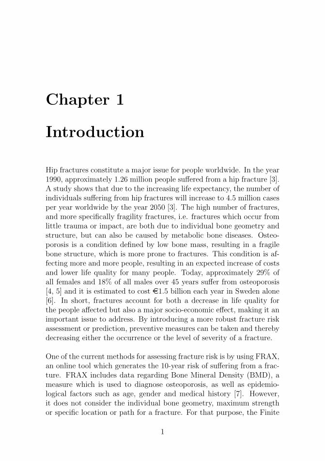
The design of the study is as follows: clinical CT-images were used togenerate subject-specific 3D-Finite element models for two human femurbones. Boundary and loading conditions were applied to resemble thosedefined in previous experiments [1]. The subject-specific finite elementmodels were used to predict fracture location and pathway and theresults were compared with experimental data [1].
1.2. DESIGN OF THE STUDY 3
Figure 1.1: Design of the study

4 CHAPTER 1. INTRODUCTION

Chapter 2
Theory
2.1 Bone
As part of the skeletal system, bones provide support and protection,allow movement, produce blood cells and act as a storage for mineralsand lipids. The human skeleton consists of 206 bones, which can be di-vided into several groups. One group is long bones, to which the femur,the thigh bone, belongs (see figure 2.1). The long shaft of the femur,which contains the marrow canal, is called the diaphysis. At each end,the epiphysis are located, the proximal located closest to the hip andthe distal located closest to the knee. The proximal femur can be seen inmore detail in figure 2.1 (b). The femoral head connects the limb to theupper body through the pelvis, and the greater and lesser trochanterare protruding areas acting as connection sites for larger ligaments andtendons. The part between the femoral head and the trochanters arereferred to as the femoral neck and is the region most commonly affectedby osteoporotic fractures [4].
5

6 CHAPTER 2. THEORY
Figure 2.1: Femur - location in the human body (a) and whole bonestructure (b)
In general, the long bones are built up of two types of bone tissue:compact (cortical) bone, and spongy (trabecular) bone. Both corticaland trabecular bone share the same basic composition, with cell-typescalled osteoblasts, osteoclasts and osteocytes. However, the two typesof bones are built up from different micro-structure depending on theirrespective function. In the cortical bone, the osteocytes are arrangedaround the so-called Haversian canal, and the lamellae oriented in thesame direction as the canal, i.e. along with the diaphysis of the bone.In trabecular bone, the lamellae create a network of branches, similarto a honeycomb-shape, called trabeculae (see figure 2.2). The purposeof these different structures of the bones is dependent on the functionsthey have. The cortical bone can, through the parallel arrangement ofthe lamellae and the much higher density, withstand large forces in thedirection of the lamellae (along the diaphysis). However, when exposedto a sideway force in relation to the lamellae orientation in cortial bone,it can quite easily break. On the other hand, the trabecular bone isconstructed in order to withstand multi-directional forces, but can ingeneral not withstand as large forces as cortical bone [4].

2.2. OSTEOPOROSIS 7
Figure 2.2: Compact and spongy bone [10]
2.2 Osteoporosis
Osteoporosis is a medical condition characterized by a decreased bonemass leading to a fragile bone structure and an increased risk of frac-tures. Osteoporosis can be a side-effect from another medical condition,but is generally a result of aging. The most common form of osteoporosisis therefore known as senile osteoporosis and affects most aging individ-uals. The normal bone loss, as an effect of aging, is an average of 0.7%bone mass decrease per year and is mostly affecting the areas whichcontain more trabecular bone, such as the femoral neck. These regionsare therefore the location where the majority of osteoporosis relatedfractures occur [5].
Osteoporosis is estimated to affect 29% of all women and 18% of allmen over the age of 45. Women, or more specifically, post-menopausalwomen, have a larger risk of suffering from fractures due to osteoporo-sis. This is due to the fact that after the entry of menopause, there isa decrease in certain hormones, which can accelerate the progression ofbone loss [4, 5]. In the year 2010, it was estimated that osteoporosisaccounted for an annual cost of e1.5 billion in Sweden alone, making itan important issue to address [6].
The current method for diagnosing osteoporosis is by measuring thebone mineral density (BMD). This is done by performing a 2D-dual-energy X-ray absorptiometry (DXA), which provides the mineral con-tent of a bone. By dividing the mineral content by the area scanned

8 CHAPTER 2. THEORY
with the 2D-DXA, a measure of the BMD is provided. With the averageBMD of a young, female reference population being x, osteoporosis isthen defined as a BMD < x-2.5 standard deviations (SD) [11].
Figure 2.3: Distribution of BMD for a female population
Figure 2.3 shows the distribution of the prevalence of osteoporosisfor a healthy female population and shows that approximately 15% ofthe population is osteopenic and 0.6% are suffering from osteoporosis[11]. Osteopenia, or low bone mass, is defined as BMD < x− 1 SD butBMD > x − 2.5 SD the mean and can be considered pre-osteoporosis.Values of BMD > x− 1 SD below the mean can be considered a normalvalue.
2.3 Fracture risk assessment
To assess the fracture risk of an individual, one method is to performa 2D-DXA, in order to get the BMD value. With this, the patient canbe categorized as normal, osteopenic or osteoporotic, and if needed, po-tential medication can be given [12].
Another current method is an online-tool called FRAX, developed atthe University of Sheffield in 2008 [7]. The purpose of FRAX is to gen-erate a 10-year prospect regarding the risk of suffering from a fracture.The tool combines the information about BMD with clinical risk factors

2.4. BONE MECHANICS 9
such as age, sex, weight, height, smoking and alcohol habits, as well asmedical history from parents.
Although the algorithms of FRAX provides promising results, thereare many improvements which can be implemented in order to increaseaccuracy. FRAX does not include any information about the bone ge-ometry, something which can be a significant factor in terms of fractureestablishment. Some suggestions of improvement to FRAX are also toinclude more clinical risk factors, another is to include personalized dataabout the maximum load a bone can withstand without fracturing [13].
2.4 Bone mechanics
Two basic measurements in mechanical testing are stress and strain.Stress (σ) is defined as force (F) distributed over an area (A) and usuallydenoted as:
σ = F/A (2.1)
with the unit N/m2 or Pascal (Pa). Strain (ε), on the other hand, isdefined as the relative deformation, i.e. the difference in length afterdeformation (L0 − L) over the original length (L0), or:
ε = (L0 − L)/L0 (2.2)
(unitless). A material parameter often used in biomechanics is the stiff-ness. The stiffness can either be extrinsic, defined as the slope of theelastic part of a load-deformation curve, or intrinsic. The intrinsic stiff-ness of a material is more commonly referred to as the Young’s modulus(E) and is defined as the slope of the elastic part of a stress-strain curve[14].
In order to capture the mechanical properties of bone, which is a highlycomplex material, several methods are available. In mechanical test-ing, the setups are usually equipped with a load cell which controls theforce to apply on a specimen, and something to produce an output interms of displacement [14]. Bending tests are one of the most commonlyused methods to test the mechanical response of samples. A three-pointbending tests is performed by placing the sample on two supports andapplying a load on the top [15] (see figure 2.4 (a)). A four-point bendingtest is very similar to a three-point bending test but with load being

10 CHAPTER 2. THEORY
applied on two locations instead of one. By placing strain gauges (SG)son specific locations of the sample, it is possible to capture the mechan-ical response in terms of strain distribution, as used in e.g. [16] (seefigure 2.4 (b)). Another method which provides a mapping of the straindistribution over an entire body is to use the method of digital imagecorrelation (DIC), further described in [1] (see figure 2.4 (c)).
Figure 2.4: Example of methods used in bone mechanics (a) Three-pointbending test [17], (b) Strain gauges [18], (c) Digital image correlation[1]. Reprinted with permission from John Wiley and Sons, Elsevier andASME
Although these types of measurements and testing methods can pro-vide accurate results, they all have some limitations when it comes tocapture the mechanical behavior of bone. The use of SGs is highly lim-ited by the number of SGs used and their specific location [15]. DICcould be considered an improvement to the use of SGs, since it can col-lect data from more points (more than 1000 points) than SGs (usually10-15 points). However, both methods are highly time consuming andthey are also limited to surface measurements.
2.4.1 Finite element bone models
The Finite Element Method (FEM) is a numerical method for approxi-mately solving differential equations. The main objective of the methodis to divide a body into a number of smaller parts, or elements, andcalculations are then performed on an element level where certain ap-proximations are made. One common approximation to be made is thata variable varies linearly in an element, even though it shows a typicalnon-linear behavior over the total body. By thereafter assembling theresults from each element, the FEM can achieve an approximated result

2.4. BONE MECHANICS 11
of the behavior of the entire body.
The simplicity of this method makes the FEM applicable on a variety ofproblems, for example heat conduction, fluid problems, torsion, bendingetc. For a more detailed description of the underlying mathematics ofFEM, the reader is referred to [19]. In recent years, the development ofFE programs has evolved with increasing computational power and anumber of softwares are available in order to solve non-linear, transient,partial differential equations [20].
A number of researchers have been using the FEM to model the me-chanical behavior of bones, without making the models subject-specific,among them e.g. [2]. However, a subject-specific model would presum-ably produce more accurate results since the e.g. strength of a boneis highly dependent of the bone geometry and the individual materialproperties. One of the first to use the FEM to predict fractures in bones,based on the subjects themselves, was J.C. Lotz et. al. [21]. They usedCT-images from two cadaver femora in order to capture the geometryof the proximal femur as well as material parameters and simulated asingle-leg-stance and a lateral fall. The results from the models, stressdistributions mapped over the entire geometry, were used to comparethe predicted data to in vitro measurements from SGs and failure loads[21]. Since J.C. Lotz et. al., several others have produced more elaboratemodels and to use FEM in biomechanics is a continuously growing area.
However, even though there are a number of models accurately de-scribing the biomechanical behavior of bones in terms of strain andstress distribution [1, 21] they do not include information about crackpropagation or fracture.
2.4.2 Finite element modeling of fractures in bone
In order to model discontinuities, such as a crack in a material, onemethod is to continuously update the mesh, by making refinements orcompletely remaking the mesh, to fit the new geometry following thediscontinuities. To avoid the need of continuously update the mesh,other methods were developed. In 1996, J.M. Melenk and I. Babuskadescribed the theory and possible fields of application for the Parti-tion of Unity Finite Element Method (PUFEM) [22]. The PUFEM is
12 CHAPTER 2. THEORY
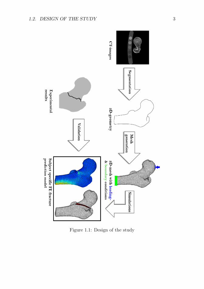
an further developed version of FEM based on the Partition of Unity,which enhances the solution space, making it possible to also handledifferential equations with strong discontinuities. By adding additionaldegrees of freedom to certain nodes, it allows a discontinuity, such as acrack, to take form while also avoiding re-meshing completely [23]. Fora more detailed description of the underlying mathematics of PUFEM,the reader is referred to section 2.5 and [22].
The introduction of PUFEM made it possible for further development ofbiomechanical modeling, where discontinuities such as cracks and frac-tures could be mathematically described. With PUFEM, the modelscould be used to produce the same output as using the standard FEM,i.e. e.g. stress and strain distributions, but in addition to this alsoparameters such as fracture energy and more accurate descriptions ofcrack paths and initiation. However, one downside of PUFEM in com-parison to the standard FEM is the need of larger computational powerand storage space.
2.5 PUFEM
A crack or failure of any material can be seen as a discontinuity inthe displacement or strain field and can be described using the strongdiscontinuity approach. Assuming a body ∂Ω0 exists and that a dis-continuity ∂Ω0d separates this body into sub-bodies which occupy thesub-domains ∂Ω0+ and ∂Ω0−. A deformation X maps the sub-domains∂Ω0+ and ∂Ω0− into their relative configurations ∂Ω+ and ∂Ω− (seefigure 2.5). With X being a material point, the resulting jump in thedisplacement field can be written as
u(X) = uc(X) +H(X)ue(X) (2.3)
where uc and ue are the regular and enhanced displacement field, re-spectively [2]. Furthermore, H represents the Heaviside function andtakes the values 0 for ∂Ω− and 1 for ∂Ω+. This means, that for ∂Ω−,the displacement of the material point X can be written as
u− = uc(X) + 0 · ue(X) = uc(X) (2.4)
and for ∂Ω+
u+ = uc(X) + 1 · ue(X) = uc(X) + ue(X) (2.5)

2.5. PUFEM 13
Figure 2.5: Strong discontinuity kinematics capturing a crack
In PUFEM, where the partition of unity is used, the general dis-placement field u can be written as
u =
nelem∑i=1
N IuIc +Hnelem∑i=1
N IuIe, (2.6)
where N I are the finite element shape functions, nelem the number ofnodes per element, H the Heaviside function and uIc and uIe are theregular and enhanced nodal displacements, respectively.
2.5.1 Cohesive crack concept
The cohesive crack concept (CCC) or cohesive zone model is a modelin which a fracture is assumed to be a gradual process where surfacesseparate from each other. The separation of surfaces is resisted by acohesive traction, and the stress (σ) will therefore first increase withincreasing surface displacement (δ) until a certain threshold called thecohesive strength (σmax) is reached. Thereafter, the stress decreasesto zero at the displacement at complete separation (δc), i.e. at thedisplacement where an open crack of the material, occurs [24]. Anintegration of the function described in figure 2.6, i.e. the area underthe graph, is equivalent to the fracture energy. The fracture energy (Gc)is the energy needed in order to achieve the separation of surfaces, i.e.to open the crack. The CCC is implemented in the present work tomodel a fracture in bone [2].

14 CHAPTER 2. THEORY
Figure 2.6: Cohesive Crack Concept
2.5.2 Fracture initiation criterion
In order to model crack or fracture initiation, a non-local version ofthe so-called Rankine Criterion can be used. The Rankine Criterionsays that failure occurs when the maximum principal stress in an ele-ment exceeds a predefined threshold, in this case the cohesive strength(σmax). The non-local Rankine criterion is based on the average stress,computed in a sphere with some determined radius. The element, lo-cated in the center of the sphere, is defined as cracked if the maximumprincipal stress in the sphere exceeds the cohesive strength (σmax). Theorientation of the crack is defined as perpendicular, i.e. the normal vec-tor (N), to the direction of the maximum principal stress.
To use a non-local fracture criteria can be considered an advantageto a local criteria since the appearing of cracks due to very local stressconcentrations can be avoided. Another advantage is that the fractureinitiation criterion becomes less mesh-dependent. By always averagingover a pre-determined volume, and not one element, which can varyin size, the results would be more consistent for different mesh sizes.Important to note is that the fracture initiation criterion only gives in-formation about the geometry of the crack, i.e. the propagated crackpath, and does not describe whether the crack has exceeded the en-ergy needed for a complete separation of materials, i.e. a crack opening[2, 25].

2.5. PUFEM 15
2.5.3 Two-step predictor-corrector algorithm
In order to track a crack propagation, a two-step predictor-correctoralgorithm has been proposed. As the name suggests, the algorithmconsists in short of two main steps: the first one is to predict the crack’spropagation according to the fracture initiation, i.e. which elementshave exceeded the criterion formulated above and therefore have poten-tial to fail, and the crack tip data. The crack tip data can be describedby the tip-point (Pt) and the tip-facet, as shown for the 2D-case in figure2.7.
Figure 2.7: Crack surface in 2D [9]. Reprinted with permission fromElsevier
In 3D, the crack-tip data, i.e. the discontinuities, can be describedby surfaces in shape of triangles or quadrilaterals. The triangles, orquadrilaterals, can be uniquely described by the point P, determinedby the crack front and located inside the discontinuity, and the normalvector N, determined by the direction of the maximum principal stress.As the predefined criterion is met by more and more elements, the crackwill propagate through the material.
16 CHAPTER 2. THEORY
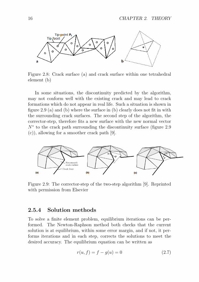
Figure 2.8: Crack surface (a) and crack surface within one tetrahedralelement (b)
In some situations, the discontinuity predicted by the algorithm,may not conform well with the existing crack and may lead to crackformations which do not appear in real life. Such a situation is shown infigure 2.9 (a) and (b) where the surface in (b) clearly does not fit in withthe surrounding crack surfaces. The second step of the algorithm, thecorrector-step, therefore fits a new surface with the new normal vectorN∗ to the crack path surrounding the discontinuity surface (figure 2.9(c)), allowing for a smoother crack path [9].
Figure 2.9: The corrector-step of the two-step algorithm [9]. Reprintedwith permission from Elsevier
2.5.4 Solution methods
To solve a finite element problem, equilibrium iterations can be per-formed. The Newton-Raphson method both checks that the currentsolution is at equilibrium, within some error margin, and if not, it per-forms iterations and in each step, corrects the solutions to meet thedesired accuracy. The equilibrium equation can be written as
r(u, f) = f − g(u) = 0 (2.7)

2.6. BACKGROUND RESEARCH FOR THIS PROJECT 17
where the the residual force r(u, f) is the difference between external,f , and internal, g(u), forces, respectively. In complete equilibrium, theresidual force would be equal to zero [26].
To solve the present finite element problem, a special case of the arc-length method is used. A pre-defined displacement, a length, is set foreach step in the solution to a control node (see values in table 3.3). Foreach step and displacement, the applied load is estimated accordinglyto meet equilibrium. If equilibrium is not met at the initial estimate ofthe load, iterations with new estimates of the load are performed untilthe absolute value of the residual force is smaller than the predefinedtolerance.
2.6 Background research for this project
This Master’s thesis is based on previous work from two research groups[1, 8, 2]. Their work will be summarized in the sections below.
Grassi et al. performed mechanical tests to simulate a single leg stancewith loading of the femur head until fracture. They used high-speedcamera recordings and DIC to obtain a full-field displacement map overthe proximal femur during mechanical tests for three human femurs.The femurs were cut approximately 5.5 cm below the lesser trochanter,and thereafter placed into a steel pot and fixated with a cold-curedepoxy-resin. A sketch of the experimental set up can be seen in figure2.10 [1]. Not only could the results obtained in this study be used as amore accurate representation of the displacement field, the results couldalso be used as validation for subject-specific FE models [8].

18 CHAPTER 2. THEORY
Figure 2.10: Sketch of the experimental setup in [1]
Grassi et al. extended their work to construct subject-specific FEmodels for the femur specimens [8]. By obtaining the geometry for eachfemur through a segmentation of clinical CT-images, a subject-specificmesh and FE model could be produced. The mesh had approximately100 000 tetrahedral elements and mechanical properties was modeledaccording to the Hounsfield units (HU)-values from CT-images. Bymodeling the same scenario as in [1], loading of the femur head up tofracture in a single leg stance, the results from [1] could be used as avalidation of the FE-predicted strains. The material model implementedwas a modified linear elastic model. In short, a material was given aspecific Young’s modulus which, when exceeding a predefined thresholdfor yield strain (εy), decreased to 5.5% of the tangent modulus. Theelement was defined as fractured when another threshold, the ultimatestrain limit (εf ), was exceeded (see figure 2.11) [8].
Figure 2.11: Material model used in [8]. Reprinted with permissionfrom Elsevier

2.6. BACKGROUND RESEARCH FOR THIS PROJECT 19
In 2007, Gasser and Holzapfel suggested using PUFEM, in order tomodel model fracture mechanical behavior of femur bone [2]. They com-bined the cohesive crack concept and the two-step predictor-correctoralgorithm (see sections 2.5.1 and 2.5.3) in order to model a crack prop-agation. Their model included a mesh of approximately 25 000 tetrahe-dral elements and modeled the entire femur as a homogeneous material.The study used the geometry from a standardized proximal femur. TheFE model was loaded on the femoral head, simulating a single leg stance,and were able to achieve results of bone failure comparable to exper-imental data in literature. Gasser and Holzapfel used a Neo-Hookeanmaterial model with the following strain-energy function:
Ψ = κ(ln(J))2/2 + µ(I : C − 3)/2 (2.8)
where κ is the bulk modulus, J is the determinant of the deformationgradient tensor, µ is the shear modulus, I the unit matrix, and C theright Cauchy Green deformation tensor.
In a Neo-Hookean material model, for given values of Young’s mod-ulus and Poisson’s ratio, the bulk and shear modulus can be describedwith the following equations:
κ =E
3(1− 2ν)(2.9)
µ =E
2(1 + ν)(2.10)
where E is the Young’s modulus, ν the Poisson’s ration, κ the bulkmodulus and µ the shear modulus.
In table 2.1 below, a comparison of [8] and [2] can be found. Thepurpose of the comparison was to capture the advantages with bothapproaches, and to create a FE-model which included the majority ofthese.

20 CHAPTER 2. THEORY
Table 2.1: Comparison of Grassi et. al. [8] and Gasser and Holzapfel[2]
AdvantageGrassi et. al.(2014, 2016)
Gasser, Holzapfel(2007)
Fine mesh xHeterogeneous material xSubject-specific models x
Fracture initiation x xFracture propagation x
Validation againstexperimental data
x

Chapter 3
Materials & methods
3.1 Material
CT-images from two male human femurs were used in this project. TheCT-images were obtained from Grassi et al. [1]. The data for thesamples used can be observed in table 3.1.
Table 3.1: Sample data [1]
Sample Age (yr) Height (cm) Weight (kg) Side (L/R)
1 58 183 85 R2 58 183 112 L
Both specimens were obtained through an ethically approved pro-tocol (ethical permission by National Authority for Medicolegal Affairs5783/2004/044/07) [1].
3.2 Segmentation of CT images
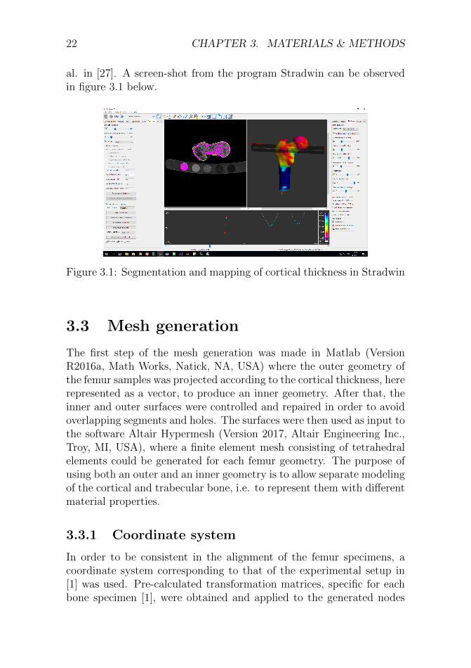
In order to obtain the three-dimensional geometry of the femurs, seg-mentation of the CT-images was performed in the software Stradwin(Version 5.3, Medical Research Imaging Group, Cambridge UniversityEngineering Department). Stradwin uses a semi-automatic segmen-tation method including thresholding to collect the three-dimensionalouter shape of the femurs. Stradwin also allows for a mapping of thethickness of cortical bone using the HU-values as described by Treece et
21
22 CHAPTER 3. MATERIALS & METHODS
al. in [27]. A screen-shot from the program Stradwin can be observedin figure 3.1 below.
Figure 3.1: Segmentation and mapping of cortical thickness in Stradwin
3.3 Mesh generation
The first step of the mesh generation was made in Matlab (VersionR2016a, Math Works, Natick, NA, USA) where the outer geometry ofthe femur samples was projected according to the cortical thickness, hererepresented as a vector, to produce an inner geometry. After that, theinner and outer surfaces were controlled and repaired in order to avoidoverlapping segments and holes. The surfaces were then used as input tothe software Altair Hypermesh (Version 2017, Altair Engineering Inc.,Troy, MI, USA), where a finite element mesh consisting of tetrahedralelements could be generated for each femur geometry. The purpose ofusing both an outer and an inner geometry is to allow separate modelingof the cortical and trabecular bone, i.e. to represent them with differentmaterial properties.
3.3.1 Coordinate system
In order to be consistent in the alignment of the femur specimens, acoordinate system corresponding to that of the experimental setup in[1] was used. Pre-calculated transformation matrices, specific for eachbone specimen [1], were obtained and applied to the generated nodes

3.4. FINITE ELEMENT MODELS 23
resulting from the mesh generation, resulting in the rotation visible infigure 3.2.
Figure 3.2: Transformation of coordinate system, (a) before, (b) after.Reprinted with permission from Elsevier [13]
3.4 Finite element models
3.4.1 Material model and material parameters
A Neo-Hookean material was used to model the bone tissue as describedin 2.6.
The modeled material was assigned the following parameter values, ac-cording to those used in [2], which for the following simulations can beseen as the ”baseline” values:
Table 3.2: Material parameters assigned to the finite element model [2]
Material parameter ValueYoung’s modulus (E) 10 GPa
Poisson’s ratio (ν) 0.35Bulk modulus (κ) 11.1 GPaShear modulus (µ) 3.7 GPa
Cohesive strength (σmax) 7.0 MPaFracture energy (Gc) 2.0 kJ/m2

24 CHAPTER 3. MATERIALS & METHODS
3.4.2 Material limits
The first model produced contained two materials, with the purposeof later being able to separately describing the cortical bone and onedescribe the trabecular bone. However, at this stage, the two materialswere modeled with the same material parameters, i.e. the model washomogeneous.
Figure 3.3: Mesh for sample 2 with 2 materials
To avoid crack formation in the distal region of the femur, a modelwith a dividing line below the lesser trochanter was also generated. Thepurpose of the dividing line was to be able to define that only the up-per material(s) were allowed to crack. The use of both a horizontaland a tilted line was investigated. The horizontal line was introducedto avoid crack formation in the proximity of the boundary conditions(BC)s (see section 3.4.3) and the tilted material line in order to avoidcrack formation due to bending in the lateral part of the shaft. Modelswith both three and four materials were tested. The models with threematerials were homogeneous (with the same material parameters in allmaterials), and the models with four materials could either be homoge-neous or heterogeneous (different material parameters for cortical andtrabecular bone, respectively).

3.4. FINITE ELEMENT MODELS 25
Figure 3.4: Mesh for sample 2, (a) horizontal line, 3 materials, (b)horizontal line, 4 materials, (c) tilted line, 3 materials, (d) tilted line, 4materials

26 CHAPTER 3. MATERIALS & METHODS
The meshes which were used for the final simulations were the fol-lowing (all with a tilted material line):
• three materials (homogeneous model), figure 3.4 (c)
• four materials (homogeneous model), figure 3.4 (d)
• four materials (heterogeneous model), figure 3.4 (d)
The purpose of having two homogeneous models, one with three andone with four materials, is to test the stability of the fracture initiationcriterion and two-step algorithm. The subroutines which implementedthese features did allow for multiple materials in a model, but a crackcould only form and propagate within the same material. That meantthat certain alterations of the subroutines had to be made in order toallow the crack to move from one material model to another. To con-firm the stability of the new subroutines, the result of the homogeneousmodel with four materials were compared to those of the homogeneousmodel with three materials. The reason for having three materials inone of the homogeneous models, and not only two, is simply to avoidre-segmentation. The initial model produced after segmentation con-sisted of two materials, resulting in a model of four materials after theintroduction of a material line. It was therefore easier to only con-vert the upper part into one material than to remake the initial model.Naturally, the lower part could also have been made into one material,but since it was not the region of interest in this project, it was notconsidered necessary.
3.4.3 Boundary conditions
Boundary conditions were applied by fixating all nodes located at themost distal part of the femoral shaft in the x- and z-directions (greenin figure 3.5) and two additional nodes fixated in all directions (x, y, z)(red in figure 3.5).
Forces were applied on the femoral head over a region correspondingto the area used in the experiment of [1], i.e. over the most superiornodes of the femoral head (blue in figure 3.5). According to the arc-length method as described in 2.5.4, the load was applied in steps, oriterations. Due to limitations of the software, it was at the current timeonly possible to perform 1 000 iterations.

3.5. SIMULATIONS 27
Figure 3.5: Illustration of boundary conditions, sample 1
3.5 Simulations
The simulations were performed using the solution method described insection 2.5.4. The control node used to apply the prescribed displace-ment were located on the lateral femoral head.
3.5.1 Software
In this project, the FEAP-software [28] was used in order to modelsubject-specific initiation and propagation of fractures in femur whensubjected to loading. Specifically, the subroutines written by Gasserand Holzapfel which implemented the fracture initiation criterion andthe fracture propagation algorithm (see sections 2.5.2 and 2.5.3) in theFEAP software were used in this project.
28 CHAPTER 3. MATERIALS & METHODS
3.5.2 Convergence study
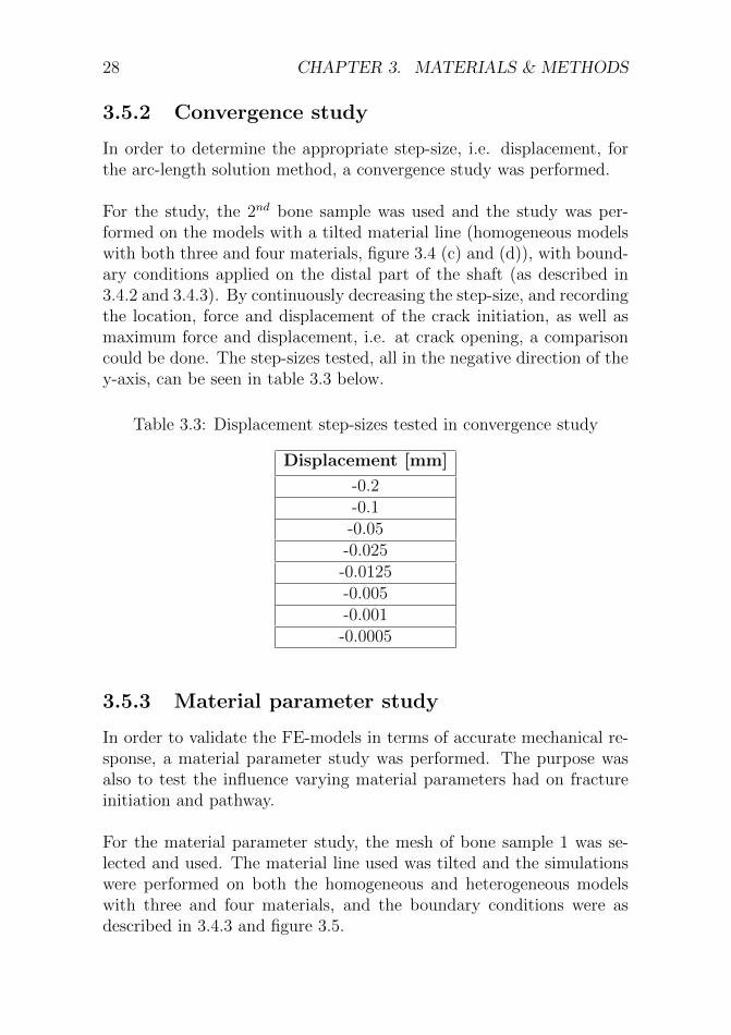
In order to determine the appropriate step-size, i.e. displacement, forthe arc-length solution method, a convergence study was performed.
For the study, the 2nd bone sample was used and the study was per-formed on the models with a tilted material line (homogeneous modelswith both three and four materials, figure 3.4 (c) and (d)), with bound-ary conditions applied on the distal part of the shaft (as described in3.4.2 and 3.4.3). By continuously decreasing the step-size, and recordingthe location, force and displacement of the crack initiation, as well asmaximum force and displacement, i.e. at crack opening, a comparisoncould be done. The step-sizes tested, all in the negative direction of they-axis, can be seen in table 3.3 below.
Table 3.3: Displacement step-sizes tested in convergence study
Displacement [mm]
-0.2-0.1-0.05-0.025-0.0125-0.005-0.001-0.0005
3.5.3 Material parameter study
In order to validate the FE-models in terms of accurate mechanical re-sponse, a material parameter study was performed. The purpose wasalso to test the influence varying material parameters had on fractureinitiation and pathway.
For the material parameter study, the mesh of bone sample 1 was se-lected and used. The material line used was tilted and the simulationswere performed on both the homogeneous and heterogeneous modelswith three and four materials, and the boundary conditions were asdescribed in 3.4.3 and figure 3.5.

3.5. SIMULATIONS 29
Cohesive strength
Simulations were performed on the meshes with varying values of thecohesive strength (σmax) and the other parameters remaining as thebaseline values (see table 3.2). The values tested can be seen in table3.4 below and are based on values from [29, 30, 31].
Table 3.4: Values of cohesive strength tested in material parameterstudy
Cohesive strength (σmax)
7 MPa20 MPa50 MPa100 MPa
Stiffness
Simulations were then performed with varying values of the Young’smodulus (E). First, the entire bone was modeled as homogeneous,i.e. all materials had the same material parameters, and the Young’smodulus varied according to the values in table 3.5a. The resultingvalues of bulk and shear moduli according to equation 2.9 and 2.10are also noted. Thereafter, the value of all material parameters of thecortical bone was fixed at the baseline level (see table 3.2), and the valuesof the Young’s modulus of the trabecular bone varied according to thevalues in table 3.5b. The variation of the values for the homogeneousvalues are based on the baseline values from [2] and results from [32].The values for the trabecular bone material are based on the maximumand minimum values presented in [33].

30 CHAPTER 3. MATERIALS & METHODS
Table 3.5: Values of Young’s modulus tested in material parameterstudy
(a) Homogeneous model (three andfour materials)
Homogeneous modelE [GPa] ν κ [GPa] µ [GPa]
5 0.35 6 210 0.35 11 420 0.35 22 730 0.35 33 11
(b) Heterogeneous model
Heterogeneous modelE [MPa] ν κ [MPa] µ [MPa]
250 0.35 278 93750 0.35 833 2781000 0.35 1111 3703000 0.35 3333 1111

Chapter 4
Results
4.1 Convergence study
The results from the convergence study regarding the step-size to beused in the arc-length method can be visualized below. Figure 4.1 showsthe distance between the crack initiation point for each value and thecrack initiation point for the smallest step-size. In figure 4.1, the valuesappear to have stabilized for the three smallest step-sizes, and no majorshift in crack initiation point can be seen. The entire convergence studywas performed on sample 2, both three and four homogeneous materials,with the material parameters as those defined as baseline values (seetable 3.2). The difference in the results between the models with threeand four materials can be explained by the different averaging methodswhich occurs when the crack formation is in the proximity of a materialline (see section 2.5.2 and 5.1 for more details).
31

32 CHAPTER 4. RESULTS
Figure 4.1: Results from convergence study, crack initiation point (inrelation to the crack initiation point of the smallest step-size, 0.0005mm) vs. step-size, sample 2
The crack initiation points as a function of step-size can also bevisualized in relation to the femoral geometry in the figure 4.2 below.For visual purposes, the element marked in the figure is the first elementat the bone surface to crack.

4.1. CONVERGENCE STUDY 33
Figure 4.2: Crack initiation point, sample 2, with (a) 3 materials, (b) 4materials
The force-displacement curves for the models tested displayed sim-ilar behavior with an initial phase of a more or less linear curve withpositive slope, followed by a sudden drop in the force. The point ofthe drop indicated the crack opening, i.e. the maximum force the bonemodel can withstand before cracking completely and the displacementat that time. The following figure, figure 4.3, shows a representativeexample of a force-displacement curve for sample 2, modeled with threehomogeneous materials. In the force-displacement curve, crack initia-tion and crack opening are indicated. In the current implementation,the subroutines do not allow to get accurate information about fracture

34 CHAPTER 4. RESULTS
energy, i.e. when the crack actually opens. What is denoted as crackopening in the figures below, is the maximum force, used as an indica-tion of crack opening based on similar behavior for existing data [1, 2].The part of the plot in figure 4.3 which follows the drop, should be con-sidered with caution. This part indicates a recovery phase after a crackopening. The increasing values indicates that there is still some partsin the structure which can bear load, for continuously increasing force.This is something which would not appear in real life and the valuesafter crack opening have therefore not been included in any analysis.
Figure 4.3: Example of a force-displacement curve, sample 2, with 3materials
Figure 4.4 shows the result of the registered forces at crack initiationand maximum force recorded, i.e. crack opening, in relation to varyingstep-sizes. The force is recorded at the nodes where the load is appliedwith load, i.e. the most superior nodes at the femoral head.

4.1. CONVERGENCE STUDY 35
Figure 4.4: Results from convergence study, force vs. step-size, sample2 (homogeneous models)
The results in figure 4.4 show a very similar behavior for the twomodels, i.e. there is a small difference in resulting force between thetwo. It can also be noted that the force required for crack initiationis close to unaffected by varying step-size. The step-size has howevera much larger impact on the maximum force recorded. From theseresults, it was concluded that a step-size of 0.005 mm would be themost appropriate to use. Further reductions of the step-size did notresults in significant changes in the predictions (see table 4.1).
Table 4.1: Convergence study, force at crack opening and force at crackinitiation for step-sizes 0.005 and 0.0005 mm
Crack initiation [N] Crack opening [N]Step-size 3 materials 4 materials 3 materials 4 materials
0.005 1550 1445 4259 43430.0005 1548 1430 4238 4368
Difference -0.13% -1.05% -0.50% +0.57%
36 CHAPTER 4. RESULTS
4.2 Material parameter study
4.2.1 Baseline model
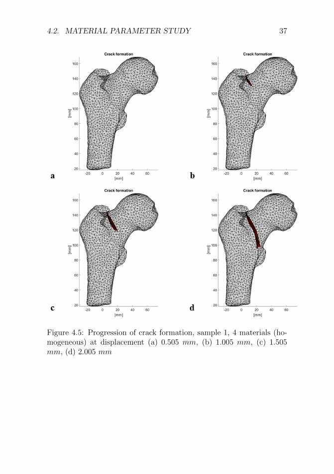
In figure 4.5 and 4.6 below, the crack formation and maximum principalstresses can be visualized. The results are from sample 1, homogeneouswith four materials, with the material parameters assigned as the base-line values. Each sub-figure shows one step in the solution, markedin the caption with the current displacement applied to the controlnode used in the arc-length method. As the crack propagates throughthe femoral neck (figure 4.5), a stress concentration clearly follows thecrack tip-point (figure 4.6). A larger stress concentration can also beseen at the lateral shaft which proves the purpose of the material line.For a better visual representation of the stress, the stresses of the nodesapplied with load, have been set to zero.
4.2. MATERIAL PARAMETER STUDY 37
Figure 4.5: Progression of crack formation, sample 1, 4 materials (ho-mogeneous) at displacement (a) 0.505 mm, (b) 1.005 mm, (c) 1.505mm, (d) 2.005 mm

38 CHAPTER 4. RESULTS
Figure 4.6: Progression of maximum principal stresses (with crack pro-gression superimposed), sample 1, 4 materials (homogeneous), at dis-placement (a) 0.505 mm, (b) 1.005 mm, (c) 1.505 mm, (d) 2.005 mm
In figure 4.7 below, the maximum principal stresses, crack formation,nodal displacements (enhanced by a factor 5 for clarifying purposes) anda plot of the elements cracked can be visualized. The prolongation ofelements in the femoral neck in figure 4.7 (c) of nodal displacementrepresents the location of the opened crack but gives the appearanceof the material being stretched. The images in figure 4.7 are from the

4.2. MATERIAL PARAMETER STUDY 39
final step of the simulation (at a displacement of 5 mm) and for thesame sample as described above, i.e. sample 1, with four materials(homogeneous) and baseline values for the material parameters.
Figure 4.7: Sample 1, 4 materials (homogeneous), (a) Maximum prin-cipal stresses, (b) Crack formation, (c) Nodal displacements (enhancedby a factor 5), (d) Elements cracked
40 CHAPTER 4. RESULTS
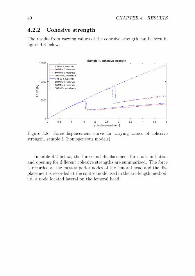
4.2.2 Cohesive strength
The results from varying values of the cohesive strength can be seen infigure 4.8 below:
Figure 4.8: Force-displacement curve for varying values of cohesivestrength, sample 1 (homogeneous models)
In table 4.2 below, the force and displacement for crack initiationand opening for different cohesive strengths are summarized. The forceis recorded at the most superior nodes of the femoral head and the dis-placement is recorded at the control node used in the arc-length method,i.e. a node located lateral on the femoral head.

4.2. MATERIAL PARAMETER STUDY 41
Table 4.2: Force and displacements at crack initiation and crack openingfor varying cohesive strength, sample 1 (homogeneous models)
(a) 3 materials
σmax[MPa]Crack initiation Crack openingForce[N]
Disp.[mm]
Force[N]
Disp.[mm]
7 1 619 0.47 4 637 1.5420 4 469 1.34 8 786 2.8150 10 396 3.39 - -100 - - - -
(b) 4 materials
σmax[MPa]Crack initiation Crack openingForce[N]
Disp.[mm]
Force[N]
Disp.[mm]
7 1 534 0.44 4 766 1.6020 4 217 1.26 8 339 2.7050 9 888 3.20 - -100 - - - -
As shown in table 4.2, no crack opening occurred for the two highestvalues of cohesive strength (50 and 100 MPa) and for the highest (100MPa), no crack occurred at all at the current displacement applied.For more details, see section 5.2.2. The onset of the crack paths for thehomogeneous models with varying cohesive strength looked similar forall values. A more accurate analysis was not possible due to the short(or non-existing) crack paths which occurred for the models with highervalues of cohesive strength. To quantify the variation of crack initiationpoint, the crack initiation point for the lowest value of cohesive strength(i.e. 7 MPa) was used as reference and the distance from the crack ini-tiation point for a cohesive strength 20 and 50 MPa was calculated.
The crack initiation point varied as a maximum of 3.23 mm for themodels with three materials (between the models with 7 and 20 MPa)and 0.0047 mm for the models with and four materials (between themodels with 7 and 50 MPa). The maximum difference in crack initia-tion point between the models of three and four materials was calculated
42 CHAPTER 4. RESULTS
as the difference of the mean of each coordinate, resulting in a maximumdifference in x-coordinate, with a value of 1.82 mm. For more details,see Appendix, table 7.1. The crack path did not noticeably change fromthe one presented for the baseline model, figure 4.5, and are thereforenot shown here.
4.2.3 Stiffness
Homogeneous model
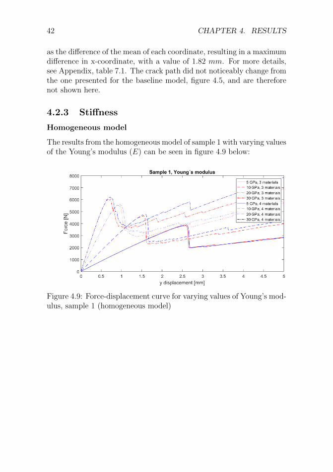
The results from the homogeneous model of sample 1 with varying valuesof the Young’s modulus (E) can be seen in figure 4.9 below:
Figure 4.9: Force-displacement curve for varying values of Young’s mod-ulus, sample 1 (homogeneous model)

4.2. MATERIAL PARAMETER STUDY 43
Table 4.3: Force and displacements at crack initiation and crack openingfor varying Young’s modulus, sample 1 (homogeneous model)
(a) 3 materials
E[GPa]Crack initiation Crack openingForce[N]
Disp.[mm]
Force[N]
Disp.[mm]
5 1 585 0.93 3 840 2.5710 1 619 0.47 4 637 1.5420 1 654 0.24 5 538 0.9330 1 643 0.16 6 035 0.67
(b) 4 materials
E[GPa]Crack initiation Crack openingForce[N]
Disp.[mm]
Force[N]
Disp.[mm]
5 1 495 0.88 3 883 2.6010 1 534 0.44 4 766 1.6020 1 550 0.22 5 641 0.9230 1 537 0.15 6 213 0.72
The crack path of the homogeneous models did not change notice-ably between neither the models with three and four materials, nor withvarying modulus compared to the models with baseline material values(figure 4.5). The difference in crack initiation point was calculated inthe same way as described in the end of section 4.2.2, with the crack ini-tiation point from the model with the lowest value of Young’s modulus(i.e. 5 GPa) as reference point. In the homogeneous model with threematerials the crack initiation point varied at a maximum with 3.23 mm(between the models with 5 and 10 GPa). For the model with fourmaterials, the corresponding value was 0.0008 mm (between the modelswith 5, 20 and 30 GPa).
The maximum difference in crack initiation point between the modelsof three and four materials was calculated as the difference of the meanof each coordinate, resulting in a maximum difference in x-coordinate,with a value of 1.90 mm. For more details, see Appendix, table 7.2.

44 CHAPTER 4. RESULTS
Heterogeneous model
The results from the heterogeneous model of sample 1 with the materialparameters of the cortical bone tissue fixed at baseline values (Young’smodulus = 10 GPa) and with varying values of the trabecular Young’smodulus (E) can be seen in figure 4.10 below:
Figure 4.10: Force-displacement curve for varying values of Young’smodulus of the trabecular bone (Young’s modulus for cortical bone fixedat 10 GPa), sample 1 (heterogeneous model)
The values of force and displacement at crack initiation can alsobe seen in table 4.4 below. Only the model with a trabecular Young’smodulus of 3 000 MPa reached a crack opening at a force of 4 044 Nand the displacement 2.54 mm. This was due to the softer trabecularmaterial in the other models (250, 750 and 1000 MPa), resulting inflatter slopes of the force-displacement curves. To reach the fractureenergy needed to achieve a crack opening, the displacement needs tobe higher. In the current case, the maximum displacement possible toapply was 5 mm, i.e. not enough to achieve a crack opening. For moredetails, see section 5.2.3.
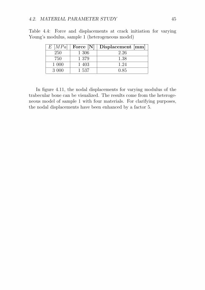
4.2. MATERIAL PARAMETER STUDY 45
Table 4.4: Force and displacements at crack initiation for varyingYoung’s modulus, sample 1 (heterogeneous model)
E [MPa] Force [N] Displacement [mm]250 1 306 2.26750 1 379 1.38
1 000 1 403 1.243 000 1 537 0.85
In figure 4.11, the nodal displacements for varying modulus of thetrabecular bone can be visualized. The results come from the heteroge-neous model of sample 1 with four materials. For clarifying purposes,the nodal displacements have been enhanced by a factor 5.

46 CHAPTER 4. RESULTS
Figure 4.11: Nodal displacements (enhanced by a factor 5) at an ap-plied displacement of 5 mm, sample 1 (heterogeneous model), (a) E =250MPa, (b) E = 750MPa, (c) E = 1000MPa, (d) E = 3000MPa
The crack paths for all the heterogeneous models exhibited a similarbehavior as the baseline model, figure 4.5, and are not therefore notshown here. Although the crack had propagated further in the modelwith the highest modulus compared to the lower, the onset of the crackslooked alike. For the crack initiation point, again calculated in the sameway as in section 4.2.2, with the crack initiation point from the modelwith the lowest value of Young’s modulus (i.e. 250 MPa) as reference

4.2. MATERIAL PARAMETER STUDY 47
point, the maximum difference was 0.0036 mm (between the modelswith 250 and 3000 MPa). For more details, see Appendix, table 7.3.

48 CHAPTER 4. RESULTS
Chapter 5
Discussion
The aim of this study was to use PUFEM in order to create subject-specific fracture predictions of the human femur. In order to reachthis aim, a subject-specific FE modeling method was combined with aPUFEM-based code that worked on homogeneous material. A conver-gence study was performed in order to find a suitable step-size in thesolution method, as well as a material parameters study to confirm theaccurate mechanical response of the models. The goal of the materialparameter study was also to assess the influence in terms of fractureinitiation point and pathway.
At the current stage, several models have been produced and tested,homogeneous models of three and four materials modeled with the samematerial parameters, and heterogeneous models of four materials withthe cortical and trabecular bone being modeled with different materialparameters. With these models, it was possible to calculate crack ini-tiation and path as well as obtaining the stress distribution and nodaldisplacements.
5.1 Convergence study
The purpose of the convergence study was to find the appropriate step-size to use in the solutions method. This was made by recording crackinitiation point, force and displacement at crack initiation as well as atcrack opening. When no significant changes were detected for decreas-ing step-size, the model had converged.
49

50 CHAPTER 5. DISCUSSION
The results from the convergence study, figure 4.1, show a clear con-vergence for the model consisting of three materials (decreasing step-size corresponding to decreasing differences in crack initiation point).For the model consisting of four materials, the results are not as clear.An increase in distance occurred between the step-sizes 0.1 and 0.05mm as well as between 0.001 and 0.0005 mm. However, the differencesbetween the step-sizes of 0.005 and 0.0005 mm are still noticeably small.
The results from the convergence study in terms of force versus vary-ing step-sizes, figure 4.4, showed very low variation in terms of forceand displacement for crack initiation (for displacement versus varyingstep-sizes, see Appendix, figure 7.1). The values of the maximum forceand displacement seem to demonstrate a slight decrease with decreasingstep-sizes. The values appear to have stabilized for the step-sizes 0.005,0.001 and 0.0005 mm, which correlates well with the results from thecrack initiation coordinates. Based on these results, three options ofstep-sizes remained; 0.005, 0.001 and 0.0005 mm. Because of the smalldifferences, and in order to save computational power and time, a step-size of 0.005 mm was used.
The purpose of testing homogeneous models with both three and fourmaterials was to test the stability of the fracture initiation criterionand two-step algorithm. The subroutines obtained from [2], which im-plemented these features in the FEAP-software, where not adapted forhandling crack propagation through multiple materials. This is a featureimplemented during this project and therefore need to be thoroughlytested and evaluated. The convergence study indicated a low, but nev-ertheless, an existing variation between the models consisting of threeand four materials. The homogeneous models consisting of three andfour materials are modeled with the exact same material parameters,and should therefore exhibit identical behavior. Even-so, a slight dif-ference can be seen between the two. These differences are most likelydue to the method of averaging in the Rankine criterion as describedin section 2.5.2. If this fracture initiation criterion is used in a modelconsisting of more than one material, there is a material line separatingthe different materials. If the element which is investigated is located inproximity of this material limit, the averaging process changes. If thesphere surrounding the element crosses a material line, the averagingonly includes those elements in the sphere, which belong to the same

5.1. CONVERGENCE STUDY 51
material as the element in question (see figure 5.1 (b)).
Figure 5.1: Averaging for the Rankine criterion in 2D over one (a) andtwo (b) materials
If changes were made to the subroutines describing the averagingmethod, so the averaging would be made independently of the numberof materials, the models are expected to behave alike.
A mesh convergence study was originally planned in order to test theappropriate mesh-size. Unfortunately, certain limitations in the subrou-tines which were used to implement the PUFEM in the FEAP software,made it impossible to perform simulations with meshes containing morethan 50 000 elements. This meant that simulations were limited to quitecoarse meshes for each bone sample, which each consisted of less than50 000 elements. To avoid the high number of elements which would bethe result in a refined mesh, the possibility to make local refinementswas also evaluated. By performing a local refinement of the femoralneck and an enlargement of the elements in the femoral shaft, head andthrochanter region, a mesh with less than 50 000 elements was achieved.However, the larger elements made the quality of the mesh poor, andsome of the details in the segmentation was lost. If no limitations inmesh-sizes were present, several different sizes could be evaluated. Asin the case of step-sizes, when no significant changes in results wouldbe detectable, the model would have converged, and a mesh-size couldbe selected. An ongoing collaboration with T.C. Gasser, is currentlyinvestigating the possibility to perform simulations with larger meshes.

52 CHAPTER 5. DISCUSSION
5.2 Material parameter study
5.2.1 Baseline model
The results from the simulations performed on sample 1, homogeneousmodel with four materials are shown in figure 4.5, 4.6 and 4.7. In figure4.5 it can be noted how the crack propagates through the femoral neckand in figure 4.6, how a stress concentration follows the crack tip. Infigure 4.6 a larger stress concentration can also be noted at the femoralshaft, proving the purpose of the material line introduces in the meshas described in section 3.4.2. Without these lines, the crack formationwould take place at the lateral femoral shaft instead of the femoral neck.
5.2.2 Cohesive strength
By increasing the cohesive strength in the different simulations, the ex-pected mechanical responses of the models are obtained. With increas-ing cohesive strength, the values of force and displacement for crackinitiation and crack opening increased accordingly (see figure 4.8 andtable 4.2). The results showed similar behavior for the models withthree and four materials, with a slight difference. Again, this differ-ence can be caused by the different methods of averaging as describedabove. For a cohesive strength of 50 and 100 MPa, neither of the mod-els showed a clear drop in force as a result of a crack opening. Thereason is that due to limitations in the implemented subroutines, it isonly possible to simulate 1 000 steps in a simulation. For the chosenstep-size of 0.005 mm, that is equivalent to a maximum displacement of5 mm. This means that if a longer simulation was possible, the modelswith the higher cohesive strength (50 and 100 MPa) would eventuallycrack as well.
For varying values of cohesive strength, a small variation in crack initi-ation point was obtained. For the models consisting of three materials,the maximum difference was 3.2 mm (between the models with a cohe-sive strength of 7 and 20 MPa), and for the model with four materialsit was 0.0047 mm (between the models with a cohesive strength of 7and 50 MPa). The largest difference in crack initiation point betweenthe models were 1.8 mm. These differences can be considered quiteinsignificant since the length of one element is approximately 3 mm.
5.2. MATERIAL PARAMETER STUDY 53
5.2.3 Stiffness
By increasing the values of the Young’s modulus for all materials inthe homogeneous models (see figure 4.9 and table 4.3), the expectedbehavior of the model in terms of mechanical response was obtained.For increasing values of Young’s modulus, the maximum force increasedaccordingly and the displacement at the same point decreased. Theforce needed for crack initiation was more or less the same for all val-ues, while the displacement needed decreased for increasing values of themodulus. The fact that the crack initiation force remained constant forvarying stiffness conforms well will the fracture initiation criteria whichis based on stress. The cohesive strength is basically a threshold whichdetermines when the crack will initiate, and since the cohesive strengthremained the same in all models tested in this section, the force neededfor crack initiation should have remained the same. The reason for thedecreasing displacement needed can be explained by the fracture energy.The fracture energy is defined as the area under the force-displacementcurve and with a steeper slope (a stiffer material), less displacement isneeded in order to reach the same area as for a flatter slope (a softermaterial).
A small variation in terms of crack initiation point was also seen withvarying Young’s modulus. The largest difference for the models con-sisting of three materials, was 3.23 mm (between the models with aYoung’s modulus of 5 and 10 GPa), and 0.0008 mm for the model withfour materials (between the models with a Young’s modulus of 5, 20and 30 GPa). The largest difference in crack initiation point betweenthe models of three and four materials was 1.90 mm.
The expected mechanical response was also obtained for the hetero-geneous model with varying values of the Young’s modulus. The forceneeded for crack initiation remained similar with increasing values, whilethe displacement decreased. However, for the models with a modulus of250, 750 and 1000 MPa, no crack opening occurred, i.e. no maximumforce and displacement at that point could be registered. This meansthat the maximum principal stress did exceed the cohesive strength(σmax), but the energy did not reach the fracture energy (Gc), as de-scribed above. Important to note is that due to limitations in the im-plemented subroutines, it is only possible to simulate 1 000 steps in asimulation. For the chosen step-size of 0.005 mm, that is equivalent to
54 CHAPTER 5. DISCUSSION
a maximum displacement of 5 mm. If the possibility to perform longersimulation existed, the models with the lower modulus would eventuallycrack as well. In addition, to obtain the energy level is at the currenttime also not possible. In order to obtain more insight into the behaviorof the models and how the crack is progressing, this would be a featurewhich would be desirable in the future.
In figure 4.11, the nodal displacements of the heterogeneous models canbe seen. With a ”softer” material, the material did not crack from thedisplacement applied on the model (5 mm), but deformed. The lowerthe modulus, the larger are the displacements, indicating a deformationof the bone (4.11 (a, b, c)). However, all models would eventually crackif a sufficiently large displacement was applied, as mentioned above. Inthe model with a modulus of 3000 MPa, figure 4.11 (d), where a crackdid occur, a ”prolongation” of the cracked elements can instead be seenand no significant bending. Even though the bone is modeled hetero-geneous, with varying values of the stiffness, the cohesive strength isthe same. A more accurate representation might be to have a differentcohesive strength for different stiffnesses.
Regarding the crack initiation point for the heterogeneous model, thelargest change for varying values of Young’s modulus was 0.0036 mm.The result that the crack initiation point is not affected by softeningthe trabecular bone, indicated that the cortical bone is responsible forcarrying the majority of the load applied. These results correspond wellwith existing results from literature which indicated the less significantimpact on bone strength of trabecular bone [34, 35]. The overall con-clusion from the material parameter study is that the crack initiationpoint seem to vary little with varying values of the material parameterschosen in this project (cohesive strength and stiffness). Neither did thecrack path seem to be much influenced by these variation. However,in some cases, the crack did not propagate far, making it hard to com-pare with longer pathways. The conclusion that the crack initiationpoint and path are not significantly influenced by varying the materialparameters chosen in this project, indicates that these are more likelyto be the results of the current boundary conditions and the bone ge-ometry. It was also noted that the models consisting of four materialsshowed less variation than the models consisting of three. This lesservariation might again been caused by the difference averaging methods

5.3. COMPARISON WITH EXPERIMENTAL DATA 55
described in section 2.5.2 and 5.1. For the models with four materials,the averaging will take place at a material limit, thus will the averag-ing be made over a smaller volume than it would in the model withthree materials. With a smaller volume to average over, the variationin maximum principal stress between the elements in that area couldbe expected to be smaller.
5.3 Comparison with experimental data
In order to validate the results obtained in this project, a comparisonwith the experimentally obtained crack path [1] and the crack initiationpoint from the numerical models [8] was made. Only small variationsin crack formation could be seen between the models, so for this com-parison, sample 1 with four materials and baseline material parameterswas used.
Figure 5.2: (a) Crack propagation, sample 1 with 4 materials, baselinematerial parameters (b) Experimentally obtained crack path (black) [1]and crack initiation from numerical models in [8] (red). Reprinted withpermission from Elsevier
Through a visual comparison, both the crack path and crack ini-

56 CHAPTER 5. DISCUSSION
tiation points seem to exhibit similar patterns. The crack path fromthe numerical models made in this project exhibits a straighter behav-ior than the experimentally obtained one. A reason for this could bethe lack of micro-structural organization of the bone in the numericalmodel. Where it in the real femur would have been cavities, is in thepresent case modeled as solid, homogeneous, matter. This makes it pos-sible for a straight crack path to develop in the model, but not in thereal femur. Another major contributor for the straight crack path is thecorrector-step of the two-step algorithm used for tracking cracks. Thisstep ensures for a smoother crack-surface.
The two red marks in figure 5.2 (b) indicate the starting points forthe crack resulting from the numerical models in [8]. The top elementcracked as a result of tension, the lower one of compression. In thepresent work, an element can only crack due to tension according to thecohesive crack concept, and the option to crack as a result of compres-sion is not implemented.
A comparison of the the force-displacement curves from the model basedon sample 1 (homogeneous model with four materials and baseline ma-terial parameters) with the results from [1] (see figure 5.3) was made.From this, it can be noted that the maximum force, and the displace-ment at this force, are significantly smaller for the first one (4 766 Nand 1.6 mm vs. 7 856 N and approximately 6.1 mm).
5.3. COMPARISON WITH EXPERIMENTAL DATA 57
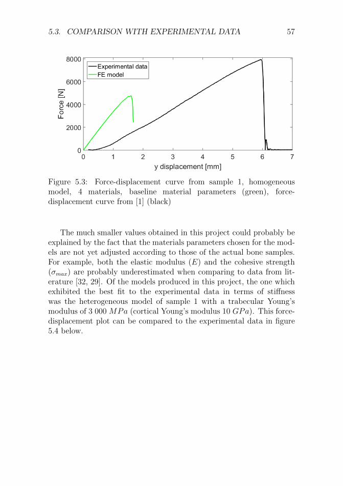
Figure 5.3: Force-displacement curve from sample 1, homogeneousmodel, 4 materials, baseline material parameters (green), force-displacement curve from [1] (black)
The much smaller values obtained in this project could probably beexplained by the fact that the materials parameters chosen for the mod-els are not yet adjusted according to those of the actual bone samples.For example, both the elastic modulus (E) and the cohesive strength(σmax) are probably underestimated when comparing to data from lit-erature [32, 29]. Of the models produced in this project, the one whichexhibited the best fit to the experimental data in terms of stiffnesswas the heterogeneous model of sample 1 with a trabecular Young’smodulus of 3 000 MPa (cortical Young’s modulus 10 GPa). This force-displacement plot can be compared to the experimental data in figure5.4 below.

58 CHAPTER 5. DISCUSSION
Figure 5.4: Force-displacement curve from sample 1, heterogeneousmodel, 4 materials, trabecular Young’s modulus 3 000 MPa (green),force-displacement curve from [1] (black)
As seen in figure 5.4, the slope of the curves, i.e. the stiffness, aremuch more similar. However, a large difference in crack opening canstill be seen, which would make the next step to adjust the values ofthe cohesive strength. In figure 5.5 below, the cohesive strength in themodel shown in 5.4 has been increased to a value of 20 MPa, resultingin the best fit to the experimental data so far.

5.4. LIMITATIONS AND FUTURE WORK 59
Figure 5.5: Force-displacement curve from sample 1, heterogeneousmodel, 4 materials, trabecular Young’s modulus 3 000 MPa, cohesivestrength 20 MPa (green), force-displacement curve from [1] (black)
Another reason for the differences between experiment and FE-models could be the different boundary conditions. Although the bound-ary conditions assigned to the models aimed at simulate those in theexperiments, the epoxy pot is missing from the models. This couldhave contributed to an overall higher stiffness, making its absence acontributor to the lower values in the models.
5.4 Limitations and future work
As a future step for this project, it would be appropriate to develop afinite element model with a more accurate representation of the materialparameters. Although the current solution of modeling the bone withtwo different materials, cortical and trabecular bone, is an improvementwhen comparing to homogeneous models, a more detailed mapping ofthe actual material parameters could be beneficial. The software Bone-mat [36] allows for a direct mapping of the elastic properties to eachfinite element by using the density from CT-images. The output is afinite element mesh containing the material properties in each elementwhich can be used as input in various finite element programs. However,at the current time, to combine Bonemat with the implemented subrou-tines in FEAP, is not possible. Due to the different averaging method

60 CHAPTER 5. DISCUSSION
which occurs when a material line is present, this would become verycumbersome since each element would be defined as a new material af-ter the use of Bonemat. From the author’s point of view, there are twooptions available: to define all elements as one material model, but toread in the element-specific material parameters from a separate file, orto change the averaging method. By altering the subroutines to allowaveraging over multiple material models, the Bonemat software couldmost probably be used.
Something which could be seen as a limitation in the current modelsis that the marrow canal is not considered. For a more realistic model,the marrow canal should be modeled with a significantly lower elasticmodulus than in the present case. However, this limitation is expectedto have a minor impact on the results in comparison to the experimentaldata provided in the project due to the mechanical setup. The part ofthe femur which would contain the marrow canal, i.e. the distal shaft, isin the mechanical tests of [1] fixed in the epoxy-pot, and would thereforebe expected to ”appear” stiffer.
This finite element model could, as mentioned above, be considered amore realistic representation of human bone than some existing models,due to the separate modeling of cortical and trabecular bone. However,the current model does not consider the actual trabeculae, the honey-comb shape. A further development of the model could therefore be aneven more thorough segmentation, where this is included. Important tonote is however that this would require micro-CT-images and a morepowerful mesh generation program. Although this could be a solutionfor obtaining a more accurate representation of bone, the method ofusing micro-CT-images would not be applicable if the fracture predic-tion were to be used on living human beings. The reason for this isthat micro-CT-images require a much higher radiation dose than whatwould be allowed in regions in the proximity of the reproductive or-gans, such as the region where the proximal femur is located. However,if the purpose of the fracture predictions would be for modeling only,the use of micro-CT-images might be appropriate. Although, studieshave shown that the trabecular part of the bone are less significant inpredictions of bone strength [34, 35], indicating that modeling of thetrabecular micro-structure would be unnecessary.

5.5. ETHICAL ASPECTS 61
In order to test the stability of the model, one option could be to trydifferent loading directions. Large fluctuations in e.g. crack initiationlocation for small changes in loading directions would indicate an in-stable model and adjustments would need to be made. Another optionwould also be to test different boundary conditions in order to confirmor contradict the assumption that the crack initiation point and pathis more influenced by those (and bone geometry) than by the materialparameters.
5.5 Ethical aspects
In this project, CT-images from two human femurs were used. Bothbone samples were previously used in the study of [1] and obtainedthrough an ethically approved protocol (ethical permission by NationalAuthority for Medicolegal Affairs 5783/2004/044/07). By re-using theseCT-images in an anonomyzed fashion, no new samples were needed andno personal data were handled.
At the current stage, the models are not sophisticated enough to beimplemented in clinics as a tool to predict fractures, but they have po-tential to be in the future. One can reflect on whether information aboutthis is beneficial or not. To get information as a patient that a fracturemay occur in a specific location and at a certain load may not be helpful.However, if this information can be used to predict generalized fracturerisk, then the patient may be treated for such with e.g. bisphosphonatesor new bone boosting drugs. Also increased physical activity, e.g. phys-ical therapy, can lead to better muscle control and thereby a reducedrisk of falling. All together this would be highly beneficial to the pa-tient. Another question to consider if the models would be implementedin clinics would be to determine who will receive this assessment. Toperform this type of fracture risk assessment, CT-images are currentlyneeded which would mean exposure to radiation for the patient. How-ever, the Biomechanics group in Lund are working to enable performingthese simulations on 2D DXA images, which would greatly reduce theradiation. Still, exposure to radiation should be avoided if possible andthe assessment would therefore be more appropriate to only offer topeople in a certain age or risk group.

62 CHAPTER 5. DISCUSSION

Chapter 6
Conclusions
The Finite Element models produced in this project are subject-specific,with both three and four materials modeled homogeneous and hetero-geneous, and are able to accurately predict the crack initiation point aswell as crack path when compared to experimental data.
The conclusion are that the models
• exhibit the expected results in terms of mechanical response withvarying material parameters.
• show that the crack initiation point and crack path are not signif-icantly influenced by varying material parameters, thus indicatingthat these are more likely the results of the currently prescribedboundary conditions and bone geometry.
• exhibit more variation in terms of crack initiation in models withthree materials than four. This indicates that the models withfour materials, modeled heterogeneously should be used for futuremodeling in order to obtain low variation and a more realisticrepresentation of bone.
63

64 CHAPTER 6. CONCLUSIONS

Bibliography
[1] Lorenzo Grassi, Sami P. Vaananen, Saber Amin Yavari, Jukka S.Jurvelin, Harrie Weinans, Matti Ristinmaa, Amir A. Zadpoor, andHanna Isaksson. Full-Field Strain Measurement During Mechani-cal Testing of the Human Femur at Physiologically Relevant StrainRates. Journal of Biomechanical Engineering, 136(11):111010,2014.
[2] T. Christian Gasser and Gerhard A. Holzapfel. A numerical frame-work to model 3-D fracture in bone tissue with application to fail-ure of the proximal femur. Solid Mechanics and its Applications,5:199–211, 2007.
[3] B Gullberg, O Johnell, and J A Kanis. World-wide Projections forHip Fracture. Osteoporos Int, 44(1997):407–413, 1997.
[4] Frederic H. Martini and Edwin F. Bartholomew. Essentials of hu-man anatomy & physiology. Pearson Education, Inc., Glenview,IL, USA, sixth edition, 2015.
[5] Vinay Kumar, Abul K. Abbas, Nelson Fausto, and Richard N.Mitchell. Robbins basic pathology. Saunders, Elsevier Inc, Philadel-phia, USA, eighth edition, 2007.
[6] A. Svedbom, E. Hernlund, M. Ivergard, J. Compston, C. Cooper,J. Stenmark, E. V. McCloskey, B. Jonsson, and J. A. Kanis. Osteo-porosis in the European Union: A compendium of country-specificreports. Archives of Osteoporosis, 8(1-2), 2013.
[7] Nelson B. Watts, Bruce Ettinger, and Meryl S. LeBoff. FRAXfacts. Journal of Bone and Mineral Research, 24(6):975–979, 2009.
65

66 BIBLIOGRAPHY
[8] Lorenzo Grassi, Sami P. Vaananen, Matti Ristinmaa, Jukka S. Ju-rvelin, and Hanna Isaksson. How accurately can subject-specific fi-nite element models predict strains and strength of human femora?Investigation using full-field measurements. Journal of Biomechan-ics, 49(5):802–806, 2016.
[9] Thomas C. Gasser and Gerhard A. Holzapfel. 3D Crack propaga-tion in unreinforced concrete. A two-step algorithm for tracking 3Dcrack paths. Computer Methods in Applied Mechanics and Engi-neering, 195(37-40):5198–5219, 2006.
[10] T.D Moran. Visual Histology - Histology Text Atlas Book, Chapter6: Bone.
[11] John A. Kanis. Diagnosis of osteoporosis and assessment of fracturerisk. Lancet, 359(9321):1929–1936, 2002.
[12] WHO. World Health Organization Scientific Group on the Assess-ment of Osteoporosis At Primary Health. 2004.
[13] Lorenzo Grassi. Femoral strength prediction using finite elementmodels. PhD thesis, Lund University, 2016.
[14] C. H. Turner and D. B. Burr. Basic biomechanical measurementsof bone: A tutorial. Bone, 14(4):595–608, 1993.
[15] Amnon Sharir, Meir Max Barak, and Ron Shahar. Whole bonemechanics and mechanical testing. Veterinary Journal, 177(1):8–17, 2008.
[16] L Cristofolini, M Viceconti, A Cappello, and A Toni. MECHAN-ICAL VALIDATION OF WHOLE BONE COMPOSITE FEMURMODELS. Journal of Biomechanics, 29(4):525–535, 1996.
[17] Olli Leppanen, Harri Sievanen, Jarkko Jokihaara, Ilari Pajamaki,and Teppo L N Jarvinen. Three-point bending of rat femur inthe mediolateral direction: Introduction and validation of a novelbiomechanical testing protocol. Journal of Bone and Mineral Re-search, 21(8):1231–1237, 2006.
[18] L. Grassi, E. Schileo, F. Taddei, L. Zani, M. Juszczyk, L. Cristo-folini, and M. Viceconti. Accuracy of finite element predictions insideways load configurations for the proximal human femur. Jour-nal of Biomechanics, 45(2):394–399, 2012.

BIBLIOGRAPHY 67
[19] Niels Ottosen and Hans Petersson. Introduction to the Finite Ele-ment Method. Pearson Education, Limited., Essex, Great Britain,1992.
[20] Robert L Taylor and Sanjay Govindjee. FEAP - A Finite ElementAnalysis Program, User manual, 2017.
[21] E. J. Lotz, J. C. Cheal and W. C. Hayes. Fracture Prediction forthe Proximal Femur Using Finite Element Models: Part I—LinearAnalysis. Journal of Biomechanics, 113(4):353–360, 1991.
[22] J. M Melenk and I Babuskab. The partition of unity finite ele-ment method: Basic theory and applications. Computer methodsin applied mechanics and englneerlng, (139):289–314, 1996.
[23] ABAQUS 6.12 Dassault Systemes R©. 10.7.1 Modeling disconti-nuities as an enriched feature using the extended finite elementmethod.
[24] B. R. K. Blackman, H. Hadavinia, Anthony J. Kinloch, and J. G.Williams. The use of a cohesive zone model to study the fractureof fibre composites and adhesively-bonded joints. InternationalJournal of Fracture, 119(1):25–46, 2003.
[25] T. Christian Gasser. Validation of 3D crack propagation in plainconcrete. Part II: Computational modeling and predictions of thePCT3D test. Computers and Concrete, 4(1):67–82, 2007.
[26] S. Krenk. Non-linear Modeling and Analysis of Solids and Struc-tures. Cambridge University Press, Cambridge, United Kingdom,2009.
[27] G. M. Treece, K. E S Poole, and A. H. Gee. Imaging the femoralcortex: Thickness, density and mass from clinical CT. MedicalImage Analysis, 16(5):952–965, 2012.
[28] Mechanics Structural Engineering, Materials, Department of Civiland Environmental Engineering, and Berkeley University of Cali-fornia. FEAP A Finite Element Analysis Program, 2017.
[29] Emer M. Feerick, Xiangyi Cheryl Liu, and Patrick McGarry.Anisotropic mode-dependent damage of cortical bone using the ex-tended finite element method (XFEM). Journal of the MechanicalBehavior of Biomedical Materials, 20:77–89, 2013.

68 BIBLIOGRAPHY
[30] Naiara Rodriguez-Florez, Alessandra Carriero, and Sandra J. She-felbine. The use of XFEM to assess the influence of intra-corticalporosity on crack propagation. Computer Methods in Biomechanicsand Biomedical Engineering, 20(4):385–392, 2017.
[31] Susan Mischinski and Ani Ural. Finite Element Modeling of Mi-crocrack Growth in Cortical Bone. Journal of Applied Mechanics,78(4):041016, 2011.
[32] Harun H. Bayraktar, Elise F. Morgan, Glen L. Niebur, Grayson E.Morris, Eric K. Wong, and Tony M. Keaveny. Comparison of theelastic and yield properties of human femoral trabecular and cor-tical bone tissue. Journal of Biomechanics, 37(1):27–35, 2004.
[33] Emil Fagelberg, Lorenzo Grassi, Per Aspenberg, and Hanna Isaks-son. Surgical widening of a stress fracture decreases local strainssufficiently to enable healing in a computational model. Interna-tional Biomechanics, 2(1):12–21, 2015.
[34] Janne E M Koivumaki, JerOme Thevenot, Pasi Pulkkinen, VolkerKuhn, Thomas M. Link, Felix Eckstein, and Timo Jamsa. Corti-cal bone finite element models in the estimation of experimentallymeasured failure loads in the proximal femur. Bone, 51(4):737–740,2012.
[35] Gerold Holzer, Gobert Von Skrbensky, Lukas A. Holzer, and Wolf-gang Pichl. Hip fractures and the contribution of cortical versustrabecular bone to femoral neck strength. Journal of Bone andMineral Research, 24(3):468–474, 2009.
[36] Insituto Ortopedico Rizzoli. Bonemat, 2015.

Appendix
Figure 7.1: Results from convergence study, displacement vs. step-size,sample 2 (homogeneous models)
69
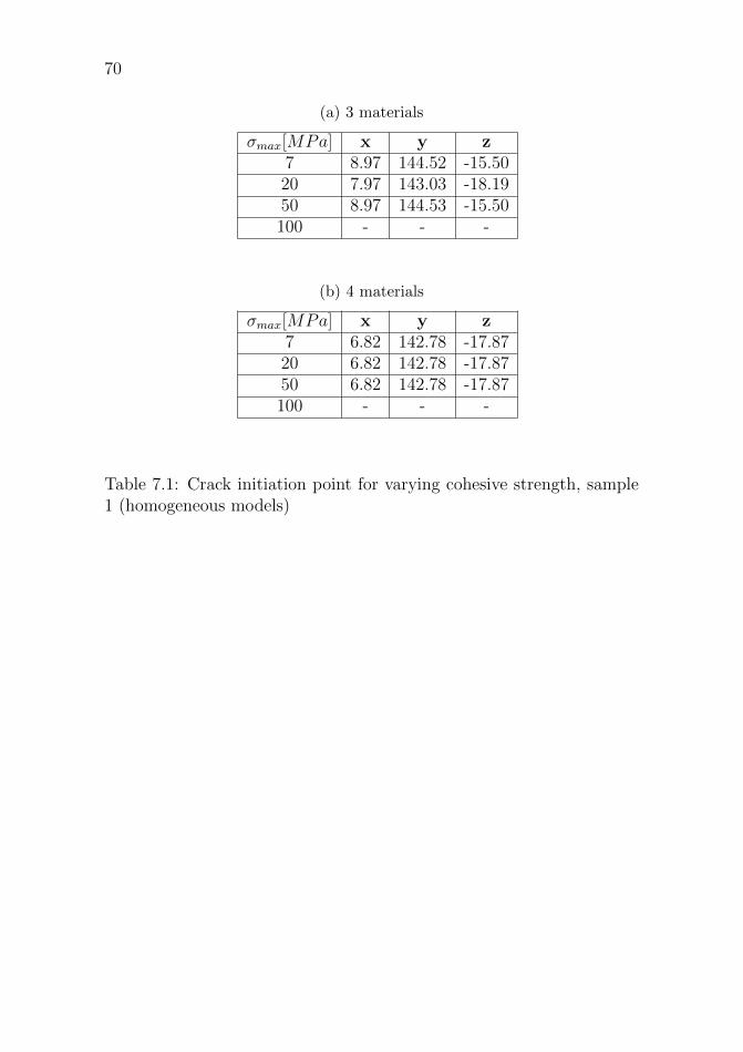
70
(a) 3 materials
σmax[MPa] x y z7 8.97 144.52 -15.5020 7.97 143.03 -18.1950 8.97 144.53 -15.50100 - - -
(b) 4 materials
σmax[MPa] x y z7 6.82 142.78 -17.8720 6.82 142.78 -17.8750 6.82 142.78 -17.87100 - - -
Table 7.1: Crack initiation point for varying cohesive strength, sample1 (homogeneous models)

71
(a) 3 materials
E [GPa] x y z5 7.97 143.03 -18.1910 8.97 144.52 -15.5020 8.97 144.52 -15.5030 8.97 144.52 -15.50
(b) 4 materials
E [GPa] x y z5 6.82 142.78 -17.8710 6.82 142.78 -17.8720 6.82 142.78 -17.8730 6.82 142.78 -17.87
Table 7.2: Crack initiation point for varying Young’s modulus, sample1 (homogeneous models)
E [MPa] x y z250 9.69 143.79 -16.12750 9.69 143.79 -16.121000 9.69 143.79 -16.123000 9.69 143.80 -16.12
Table 7.3: Crack initiation point for varying Young’s modulus, sample1 (heterogeneous models)