PREDICTION OF DOWNPULL ON HIGH HEAD GATES USING

COMPUTATIONAL FLUID DYNAMICS

A THESIS SUBMITTED TO

THE GRADUATE SCHOOL OF NATURAL AND APPLIED SCIENCES

OF

MIDDLE EAST TECHNICAL UNIVERSITY

BY

MEHMET AKIŞ UYSAL

IN PARTIAL FULLFILLMENT OF THE REQUIREMENTS

FOR

THE DEGREE OF MASTER OF SCIENCE

IN

CIVIL ENGINEERING

JANUARY 2014

Approval of the thesis:

PREDICTION OF DOWNPULL ON HIGH HEAD GATES USING

COMPUTATIONAL FLUID DYNAMICS

Submitted by MEHMET AKIŞ UYSAL in partial fulfillment of the requirements for the

degree of Master Science in Civil Engineering Department, Middle East Technical

University by,

Prof. Dr. Canan Özgen

Dean, Graduate School of Natural and Applied Sciences ____________

Prof. Dr. A. Cevdet Yalçıner

Head of Department, Civil Engineering ____________

Assoc. Prof. Dr. Mete Köken

Supervisor, Civil Engineering Dept., METU ____________

Prof. Dr. İsmail Aydın

Co-Supervisor, Civil Engineering Dept., METU ____________

Examining Committee Members

Prof. Dr. Zafer Bozkuş

Civil Engineering Dept., METU ____________

Assoc. Prof. Dr. Mete Köken

Civil Engineering Dept., METU ____________

Prof. Dr. İsmail Aydın

Civil Engineering Dept., METU ____________

Assoc. Prof. Dr. Şahnaz Tiğrek

Civil Engineering Dept., METU ____________

Assoc. Prof. Dr. Funda Kurtuluş

Aerospace Engineering Dept., METU ____________

Date: 29 January 2014

iv

I hereby declare that all information in this document has been obtained and

presented in accordance with academic rules and ethical conduct. I also declare that,

as required by these rules and conduct, I have fully cited and referenced all material

and results that are not original to this work.

Name, Last name : Mehmet Akış UYSAL

Signature :

v

ABSTRACT

PREDICTION OF DOWNPULL ON HIGH HEAD GATES USING

COMPUTATIONAL FLUID DYNAMICS

Uysal, Mehmet Akış

M.Sc., Department of Civil Engineering

Supervisor: Assoc. Prof. Dr. Mete KÖKEN

Co-Supervisor: Prof. Dr. İsmail AYDIN

January 2014, 78 Pages

For design purposes it is important to predict the downpull forces on the tunnel gates

installed in the intake of a hydropower plant. In this study downpull forces on the gates

are evaluated for different closure rates and for different gate lip geometries using

computational fluid dynamics and the results are compared to an existing experimental

study. Commercial ANSYS FLUENT software is used in the calculations. It is found that

downpull coefficients obtained from computational study showed good agreement with

the values calculated from the existing experimental study.

Keywords: Downpull, gate lip, computational fluid dynamics, pressure distribution

vi

ÖZ

HİDROLİK KAPAKLARDAKİ HİDRODİNAMİK YÜKLERİN HESAPLAMALI

AKIŞKANLAR DİNAMİĞİ KULLANILARAK BELİRLENMESİ

Uysal, Mehmet Akış

Yüksek Lisans, İnşaat Mühendisliği Bölümü

Tez Yöneticisi: Doç. Dr. Mete KÖKEN

Ortak Tez Yöneticisi: Prof. Dr. İsmail AYDIN

Ocak 2014, 78 Sayfa

Hidroelektrik santrallerin su alma yapısında bulunan hidrolik kapaklar üzerinde oluşan

hidrodinamik yüklerin belirlenmesi kapağın tasarımı için önem teşkil etmektedir. Bu

çalışmada, kapaklara etkiyen hidrodinamik yükler farklı kapak açıklıklarında ve farklı

kapak dudak geometrileri için hesaplamalı akışkanlar dinamiği kullanılarak incelenmiş ve

sonuçlar mevcut bir deneysel çalışma ile karşılaştırılmıştır. Hesaplamalarda ticari ANSYS

FLUENT yazılımı kullanılmıştır. Hesaplamalı yöntemden elde edilen aşağı çekme kuvvet

katsayılarının mevcut deneysel çalışma sonuçları ile uyum içerisinde olduğu bulunmuştur.

Anahtar Kelimeler: Aşağı çekme kuvveti, kapak dudağı, hesaplamalı akışkanlar dinamiği,

basınç dağılımı

vii

ACKNOWLEDGEMENTS

The author would like to express his gratitude to supervisor Assoc. Prof. Dr. A. Mete

Köken and co-supervisor Prof. Dr. İsmail Aydın for their guidance, advice, criticism,

encouragements and insight throughout the research.

viii

TABLE OF CONTENTS

ABSTRACT ................................................................................................................. V

ÖZ ............................................................................................................................... VI

ACKNOWLEDGEMENTS ........................................................................................ VII

TABLE OF CONTENTS...........................................................................................VIII

LIST OF FIGURES ...................................................................................................... X

LIST OF TABLES ....................................................................................................XIII

LIST OF SYMBOLS AND ABBREVIATIONS ...................................................... XIV

CHAPTERS

1. INTRODUCTION ................................................................................................. 1

1.1 Description of the Problem ............................................................................. 1

1.2 Scope and Aim of the Study ........................................................................... 3

1.3 Literature Review........................................................................................... 3

2. BACKGROUND ................................................................................................... 7

2.1 Multipurpose Hydraulic Model ...................................................................... 7

2.2 Forces on a Hydraulic Gate .......................................................................... 12

2.3 Downpull Force Coefficient ......................................................................... 13

2.4 Experimental Results ................................................................................... 14

2.4.1 Pressure Distributions on the Gate Lip ................................................... 14

2.4.2 Lip Downpull Coefficient—Reynolds Number Relationship .................. 19

2.4.3 Lip Downpull Coefficient as a Function of the Gate Opening and the Lip

Angle ..................................................................................................... 22

3. COMPUTATIONAL MODEL ............................................................................ 25

3.1 Mesh Generation with GAMBIT .................................................................. 25

3.1.1 Forming the Geometry .......................................................................... 25

ix

3.1.2 Forming the Grid.................................................................................... 28

3.1.3 Clustering .............................................................................................. 29

3.1.4 Near Wall Mesh ..................................................................................... 31

3.1.5 Mesh Size .............................................................................................. 32

3.1.6 Boundary Conditions ............................................................................. 33

3.2 ANSYS FLUENT Setup and Simulations ..................................................... 33

3.2.1 Importing the Mesh ................................................................................ 33

3.2.2 Scaling, Defining the Material and Gravity ............................................ 33

3.2.3 Turbulence Model .................................................................................. 34

3.2.4 Boundary Conditions ............................................................................. 35

3.2.5 Residuals ............................................................................................... 36

3.2.6 Simulations ............................................................................................ 37

3.3 Selecting the Domain Size ............................................................................ 38

3.4 Grid Dependence Study ................................................................................ 40

3.5 Computational Results .................................................................................. 41

3.5.1 Processing for Results ............................................................................ 41

3.5.2 Computational Models ........................................................................... 42

3.5.3 Pressure Distributions on the Gate Lip ................................................... 45

3.5.4 Lip Downpull Coefficient—Reynolds Number Relationship .................. 50

3.6 Comparison of Selected Flow Properties ...................................................... 53

3.6.1 Effect of Gate Opening .......................................................................... 53

3.6.2 Effect of Lip Angle ................................................................................ 59

3.6.3 Effect of Discharge ................................................................................ 64

3.7 Lip Downpull Coefficient as a Function of the Gate Opening and the Lip

Angle ........................................................................................................... 69

3.8 Comparison of Experimental and Computational Values .............................. 72

4. CONCLUSION .................................................................................................... 75

REFERENCES ............................................................................................................ 77

x

LIST OF FIGURES

FIGURES

Figure 2.1 Views from hydraulic model (Aydin et al., 2003) .......................................... 8

Figure 2.2 Experimental setup (Aydin et al., 2003) ........................................................ 9

Figure 2.3 Details of gate region (Aydin et al., 2003) ................................................... 10

Figure 2.4 Gate lip details (Aydin et al., 2003) ............................................................. 11

Figure 2.5 Pressure distribution on gate lip, Lip A (θ=26.5°). (Aydin et al., 2003) ....... 15

Figure 2.6 Pressure distribution on gate lip, Lip B (θ=36.7°). (Aydin et al., 2003) ....... 16

Figure 2.7 Pressure distribution on gate lip, Lip C (θ=44.7°). (Aydin et al., 2003) ....... 17

Figure 2.8 Pressure distribution on gate lip, Lip D (θ=51.6°). (Aydin et al., 2003) ....... 18

Figure 2.9 Downpull coefficient—Reynolds number relationship, y=0.1 (Aydin et al.,

2003) ........................................................................................................................... 19

Figure 2.10 Downpull coefficient—Reynolds number relationship, y=0.2 (Aydin et al.,

2003) ........................................................................................................................... 20

Figure 2.11 Downpull coefficient—Reynolds number relationship, y=0.4 (Aydin et al.,

2003) ........................................................................................................................... 20

Figure 2.12 Downpull coefficient—Reynolds number relationship, y=0.6 (Aydin et al.,

2003) ........................................................................................................................... 21

Figure 2.13 Downpull coefficient—Reynolds number relationship, y=0.8 (Aydin et al.,

2003) ........................................................................................................................... 21

Figure 2.14 Downpull coefficient as a function of gate opening and gate lip angle (Aydin

et al., 2003) ................................................................................................................. 23

Figure 3.1 Geometry formed by GAMBIT ................................................................... 27

Figure 3.2 Block based modelling ................................................................................ 28

Figure 3.3 Mesh refinement ......................................................................................... 30

xi

Figure 3.4 Mesh around the gate .................................................................................. 31

Figure 3.5 Mesh around gate and parts of upstream and downstream ........................... 31

Figure 3.6 Near-wall mesh ........................................................................................... 32

Figure 3.7 Residuals..................................................................................................... 38

Figure 3.8 Maximum system discharge (Aydin et al., 2003) ......................................... 43

Figure 3.9 Pressure distribution on gate lip, Lip A (θ=26.5°). (Computational) ............ 46

Figure 3.10 Pressure distribution on gate lip, Lip B (θ=36.7°). (Computational) ........... 47

Figure 3.11 Pressure distribution on gate lip, Lip C (θ=44.7°). (Computational) ........... 48

Figure 3.12 Pressure distribution on gate lip, Lip D (θ=51.6°). (Computational) .......... 49

Figure 3.13 Downpull coefficient—Reynolds number relationship, y=0.1

(Computational) ........................................................................................................... 50

Figure 3.14 Downpull coefficient—Reynolds number relationship, y=0.2

(Computational) ........................................................................................................... 51

Figure 3.15 Downpull coefficient—Reynolds number relationship, y=0.4

(Computational) ........................................................................................................... 51

Figure 3.16 Downpull coefficient—Reynolds number relationship, y=0.6

(Computational) ........................................................................................................... 52

Figure 3.17 Downpull coefficient—Reynolds number relationship, y=0.8

(Computational) ........................................................................................................... 52

Figure 3.18 Velocity magnitude distribution for (A) θ=26.5°, y=0.1, Q=0.0295 m3/s, (B)

θ=26.5°, y=0.5, Q=0.1107 m3/s, (C) θ=26.5°, y=0.9, Q=0.1216 m3/s............................ 55

Figure 3.19 Velocity profiles under the gate section for y=0.1, y=0.5 and y=0.9........... 56

Figure 3.20 Streamlines for (A) θ=26.5°, y=0.1, Q=0.0295 m3/s, (B) θ=26.5°, y=0.5,

Q=0.1107 m3/s, (C) θ=26.5°, y=0.9, Q=0.1216 m3/s ..................................................... 57

Figure 3.21 Turbulent Kinetic Energy for (A) θ=26.5°, y=0.1, Q=0.0295 m3/s, (B)

θ=26.5°, y=0.5, Q=0.1107 m3/s, (C) θ=26.5°, y=0.9, Q=0.1216 m3/s............................ 58

Figure 3.22 Velocity magnitude distribution for (A) θ=26.5°, y=0.4, Q=0.0947 m3/s, (B)

θ=36.7°, y=0.4, Q=0.0997 m3/s, (C) θ=44.7°, y=0.4, Q=0.0955 m3/s, (D) θ=51.6°, y=0.4,

Q=0.0953 m3/s ............................................................................................................. 60

xii

Figure 3.23 Velocity profiles under the gate section for θ=26.5°, θ=36.7°, θ=44.7° and

θ=51.6°........................................................................................................................ 61

Figure 3.24 Streamlines for (A) θ=26.5°, y=0.4, Q=0.0947 m3/s, (B) θ=36.7°, y=0.4,

Q=0.0997 m3/s, (C) θ=44.7°, y=0.4, Q=0.0955 m3/s, (D) θ=51.6°, y=0.4, Q=0.0953 m3/s

.................................................................................................................................... 62

Figure 3.25 Turbulent Kinetic Energy for (A) θ=26.5°, y=0.4, Q=0.0947 m3/s, (B)

θ=36.7°, y=0.4, Q=0.0997 m3/s, (C) θ=44.7°, y=0.4, Q=0.0955 m3/s, (D) θ=51.6°, y=0.4,

Q=0.0953 m3/s............................................................................................................. 63

Figure 3.26 Velocity magnitude distribution for (A) θ=51.6°, y=0.2, Q=0.0075 m3/s, (B)

θ=51.6°, y=0.2, Q=0.0343 m3/s, (C) θ=51.6°, y=0.2, Q=0.0487 m3/s ........................... 65

Figure 3.27 Velocity profiles under the gate section for Q=0.0075 m3/s, Q=0.0343 m3/s

and Q=0.0487 m3/s ...................................................................................................... 66

Figure 3.28 Streamlines for (A) θ=51.6°, y=0.2, Q=0.0075 m3/s, (B) θ=51.6°, y=0.2,

Q=0.0343 m3/s, (C) θ=51.6°, y=0.2, Q=0.0487 m3/s .................................................... 67

Figure 3.29 Turbulent Kinetic Energy for (A) θ=51.6°, y=0.2, Q=0.0075 m3/s, (B)

θ=51.6°, y=0.2, Q=0.0343 m3/s, (C) θ=51.6°, y=0.2, Q=0.0487 m3/s ........................... 68

Figure 3.30 Downpull coefficient as a function of the gate lip angle and the gate opening

(Computational) .......................................................................................................... 71

Figure 3.31 Downpull coefficient as a function of the gate lip angle and the gate opening

(Computational and experimental comparison) ............................................................ 74

xiii

LIST OF TABLES

TABLES

Table 2.1 Gate lip angles .............................................................................................. 11

Table 3.1 Material Definition ....................................................................................... 34

Table 3.2 Turbulence Model ........................................................................................ 35

Table 3.3 Wall Roughness Properties ........................................................................... 36

Table 3.4 System Configurations ................................................................................. 37

Table 3.5 Variation in KL for different upstream lengths .............................................. 39

Table 3.6 Variation in KL for different downstream lengths ......................................... 39

Table 3.7 Grid points and KL comparison ..................................................................... 41

Table 3.8 Simulations carried out (θ=26.5° and θ=36.7°) ............................................. 44

Table 3.9 Simulations carried out (θ=44.7° and θ=51.6°) ............................................. 44

xiv

LIST OF SYMBOLS AND ABBREVIATIONS

2D Two dimensional

3D Three dimensional

A Cross sectional area of the gate on horizontal plane

AhL Horizontally projected area of the gate lip

CFD Computational fluid dynamics

d/s Downstream

DP Downpull force on the gate

e Gate opening

e0 Tunnel height

g Gravitational acceleration

H Operating head on the gate bottom

H1 Reservoir water level

h2 Water level in the gate

h2* Piezometric head just upstream from the gate

h3 Water level in gate chamber

H4 Tail water level

hl̅ Average piezometric head acting on the gate lip

hp Piezometric head of the gate lip

KL Downpull force coefficient

p Pressure

Q Discharge

r Radius of the curvature of the gate lip entrance

Re Reynolds number

Rg Reynolds number under the gate lip cross section

xv

s Distance along inclined surface of the gate lip

TKE Turbulent kinetic energy

u/s Upstream

Ug Average velocity under the gate lip cross section

y Dimensionless gate opening (e/e0)

y+ Dimensionless wall distance

γw Specific weight of water

θ Lip angle

xvi

1

CHAPTER 1

INTRODUCTION

1.1 Description of the Problem

Rectangular cross-sectioned vertical leaf gates are commonly used in large cross-sectional

conduits, such as penstocks, which is the intake structure that controls water flow and

delivers water to hydraulic turbines. These gates are used for discharge control and

emergency closure operations. Vertical leaf gates are widely favored because they are

easily constructed, installed and easy on maintenance, comparing to the other types of

gates.

Because of being operated mostly under high heads, these vertical gates are under serious

forces while operating, which can be described as hydrodynamic loading, uplift or

downpull. The high speed water passing under the gate may lead to strong vibration

problems on the gate and on the hoisting mechanisms. These forces depend on several

parameters, including variables such as pipe and gate geometry.

It is a known fact that the bottom gate geometry plays an important role while predicting

these forces. The bottom of the gate, also known as the “gate lip” has a great influence on

several factors, such as cavitation damage on the gate, gate vibrations, downpull and uplift

forces on the gate and the discharge coefficient.

Many studies have been carried out in order to eliminate cavitation damage and vibrations,

minimize downpull or uplift and maximize the discharge coefficient. Among these

mentioned factors, downpull is considered to be of great importance.

2

Downpull forces on the gate occur by a reduced pressure while a fluid flows under the

gate. Since these forces act in the closing direction of the gate, the main concern arises for

the hoisting equipment of the gate. The hoist mechanism need to withstand the weight of

the gate and the downpull. In other words, hydrodynamic downpull determines the hoist

capacity of the gate, since the hoisting equipment plus frictional forces need to resist

downpull forces and weight of the gate. Occasionally, an uplift may occur if there is a

negative downpull, which may result in failure of gate closure if the gate is not heavy

enough, thus not sufficient to withstand this uplift force.

In order to determine the downpull, a pressure distribution profile on the gate has to be

measured or predicted. Studies show that the downpull on the gate is affected by both the

geometry of the gate and the rate of flow passing under the gate.

An easy to use lip downpull coefficient was introduced as a function of the lip angle and

the gate opening (Aydin et al., 2006). This dimensionless coefficient was calculated for

different gate lips and openings. Data coming from these experiments were summarized

as a function of lip angle and the gate opening and this function was intended to be used

in the prediction of downpull forces.

For investigating the effects of downpull, small scale model experiments have been done

for a long period of time. This approach generally results in high costs, measurement

difficulties, scaling problems and depends on the availability of equipment. Again, due to

the complexity and nonlinearity of the governing equations, the analytical approach is also

not considered as an advantageous approach compared to the experimental models.

On the other hand, numerical methods are considered to be notable approaches in the

recent years. As a result of advancements in computational power, computational fluid

dynamics (CFD) became more of a great importance and these advancements led a great

progression on this approach. As a result, numerical simulations became a major

approach, especially since the development of capable software.

3

1.2 Scope and Aim of the Study

This study is an attempt to validate results from experimental studies, carried out by Aydin

et al. (2002, 2003, 2006), which experiments were conducted in the Hydromechanics

Laboratory of Civil Engineering Department at METU.

The aim of the thesis is to examine pressure distribution on the gate lips for different lip

angles and gate openings with variable discharges using computational fluid dynamics,

with the aid of commercial GAMBIT and ANSYS FLUENT software and to compare the

results coming from the experimental setup of the system.

A dimensionless downpull force coefficient will be obtained from computational

calculations and will be compared to the downpull force coefficient coming from the

original experiments. Previous experimental study on this subject showing all steps will

be summarized for better understanding the concept.

This thesis is intended to demonstrate the potential use of computational fluid dynamics

by validating results with the experimental data.

1.3 Literature Review

Hydrodynamic loadings on hydraulic gates were investigated on hydraulic models.

Variables measured from hydraulic models were represented by graphics using

dimensionless parameters and are used to predict hydrodynamic loadings (Naudascher

1986, 1991). For this purpose, empirical formulas were also offered (Naudascher 1991).

A one-dimensional analysis of the discharge passing under a gate and downpull acting on

the same gate was presented by Naudascher et al. (1964, 1986).

It is claimed that geometrical characteristics of the gates such as operating head, gate

opening and bottom gate geometry, have a great influence on net downpull on a high head

vertical leaf gate (Sagar, 1977). In addition to geometry, boundary layers and turbulence

4

have effects on the downpull on the gate. Sagar stated that gate hoist capacity must be

determined precisely in order to ensure a risk-free closure of the gates.

A numerical analysis for calculating viscous flows controlled by a vertical lift gate and

hydrodynamic forces acting on the gate was developed by Amorim and Andrade (1999).

The numerical solution is obtained from the incompressible Navier-Stokes equations and

turbulence effects are simulated by a k-ε turbulence model. After completing simulations

with the numerical model, Amorim and Andrade compared results with available

experimental data at various opening positions.

Aydin (2002) investigated pressure drop and consecutive air demand behind high head

gates during emergency closure by physical and mathematical models. Aydin formed a

mathematical model for the unsteady flow due to closing gate by applying the integral

continuity and energy equations on control volumes upstream and downstream of the gate.

Hydrodynamic loadings acting on closing high head leaf gates, are studied experimentally

on hydraulic models and a mathematical model is developed and published as a part of

the research project titled as “Hydrodynamic Downpull on Closing Hydraulic Gates”

(Aydin et al., 2003).

Experimental work on downpull force on gates installed in the intake structures of

hydroelectric power plants including lip pressure distribution measurements and direct

weighing of downpull are presented by Aydin et al. (2006).

Akoz et al. (2009) have conducted laboratory experiments to measure the velocities of a

2D open channel flow under a sluice gate and carried out simulations using computational

fluid dynamics. Akoz had used different mesh sizes to investigate the effects of the mesh

size and compared k-ε and k-ω turbulence models for the same model. Akoz found out

that k-ε turbulence model has predicted the velocity field more accurate and faster by

means of simulation time, than the k-ω model.

5

Dargahi (2010) investigated the discharge characteristics of a bottom outlet with a moving

gate by FLOW-3D software. Dargahi used experimental results for an existing scale

model and measured pressurized and free-surface flow features. Dargahi found out that

the velocity and pressure distributions were predicted by the numerical analysis within a

maximum error of 2.6% and 10%, respectively.

6

7

CHAPTER 2

BACKGROUND

2.1 Multipurpose Hydraulic Model

All experiments summarized in this chapter were conducted by Aydin et al. in 2003, as a

part of a research project supported by METU and TÜBİTAK. The results were presented

in the report which was published in 2003.

For studying the effects of hydrodynamic downpull on different gate lips and gate

openings, a physical model for a typical intake structure was constructed as the

multipurpose hydraulic model by Aydin et al. (2003). All experiments were conducted on

this model. The general view of the model is shown in Figure 2.1 and the details are shown

in Figure 2.2 (not scaled).

Starting from the upstream, system consists of a reservoir, an intake region, 0.30 m x 0.24

m rectangular cross-sectioned gate area, a ventilation shaft, transition from rectangular to

circular cross section, circular shaped penstock, a control valve representing a turbine and

an open channel which is used for measuring the tail water level and the discharge. The

parts of the model which are observed are made of transparent Plexiglass material.

In the model, H1 represents the reservoir water level, h2 the water level in the gate, h3

shows the water level in gate chamber and H4 shows the tail water level. Cross sectional

tunnel height and gate opening are represented by e0 and e, respectively. The upstream

part, from reservoir to gate, is named as the intake structure, area near the gate is named

as gate area and the distance from gate to turbine valve is named as the penstock. The

details of the gate region are shown in Figure 2.3.

8

Figure 2.1 Views from hydraulic model (Aydin et al., 2003)

9

Fig

ure

2.2

Exper

imenta

l se

tup (

Ayd

in e

t al.,

2003)

10

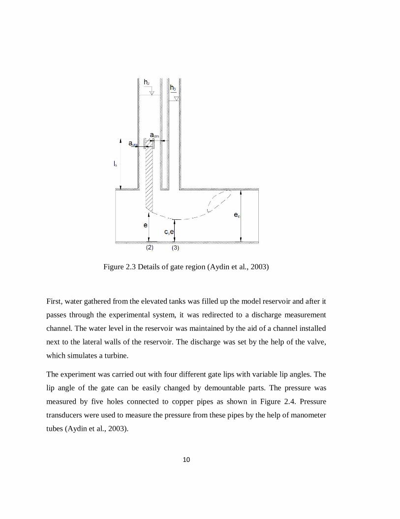
Figure 2.3 Details of gate region (Aydin et al., 2003)

First, water gathered from the elevated tanks was filled up the model reservoir and after it

passes through the experimental system, it was redirected to a discharge measurement

channel. The water level in the reservoir was maintained by the aid of a channel installed

next to the lateral walls of the reservoir. The discharge was set by the help of the valve,

which simulates a turbine.

The experiment was carried out with four different gate lips with variable lip angles. The

lip angle of the gate can be easily changed by demountable parts. The pressure was

measured by five holes connected to copper pipes as shown in Figure 2.4. Pressure

transducers were used to measure the pressure from these pipes by the help of manometer

tubes (Aydin et al., 2003).

11

Figure 2.4 Gate lip details (Aydin et al., 2003)

Four different lip angles were studied, which are considered to be covering complete

practical range and shown in Table 2.1.

Table 2.1 Gate lip angles

Lip Symbol n (cm) Lip angle, θ (degrees)

A 2 26.5

B 3 36.7

C 4 44.7

D 5 51.6

12

2.2 Forces on a Hydraulic Gate

Hydraulic gates with large cross-sectional area are subjected to several forces during their

operation. Normal load case of a hydraulic gate generally consists of frictional force,

hydrodynamic forces, dead weight, buoyant forces, transit loads and driving forces

(Erbisti, 2004).

A fully closed hydraulic gate is balanced in horizontal forces and is only subjected to

buoyant forces by means of vertical forces. The hydrostatic balance is disturbed if a

hydraulic gate is partially opened and the flow beneath the gate reaches high velocities

and reduces the pressure, which causes a non-uniform distribution of piezometric head

around the gate. Large hydrodynamic forces occur as these velocities reaches higher

values, hence leading an increase in the pressure difference (Erbisti, 2004).

The pressure difference occurring at the gate bottom causes a vertical force, which is

called the downpull force. Reducing hoist capacity by minimizing downpull, is the main

objective of many gate designers and researchers throughout the years (Sagar, 2000). Gate

downpull is determined by using an equation such as:

DP=γw. KL.A.H (2.1)

where

DP = Downpull force on the gate

γw = Specific weight of water

KL = Downpull force coefficient

A = Cross-sectional area of the gate on horizontal plane

H = Operating head on the gate bottom

13

2.3 Downpull Force Coefficient

Base variables that downpull force coefficient depends on are the lip angle, θ,

dimensionless gate opening, y (e/e0) and the system discharge, Q. If a dimensionless

coefficient is used instead of downpull force and Reynolds number for discharge, all

variables will become dimensionless. The measured piezometric head distributions are

used to estimate this dimensionless downpull coefficient.

KL =h2

∗ − hl̅

Ug2

2g

(2.2)

where h2∗ is the piezometric head just upstream from the gate and Ug is the average velocity

under the gate lip cross section.

hl̅ is defined as the average piezometric head acting on the gate lip and found from the

equation;

hl̅ =∫ hpdAhL

AhL (2.3)

where hp is the piezometric head and AhL is the horizontally projected area of the gate lip.

14

2.4 Experimental Results

2.4.1 Pressure Distributions on the Gate Lip

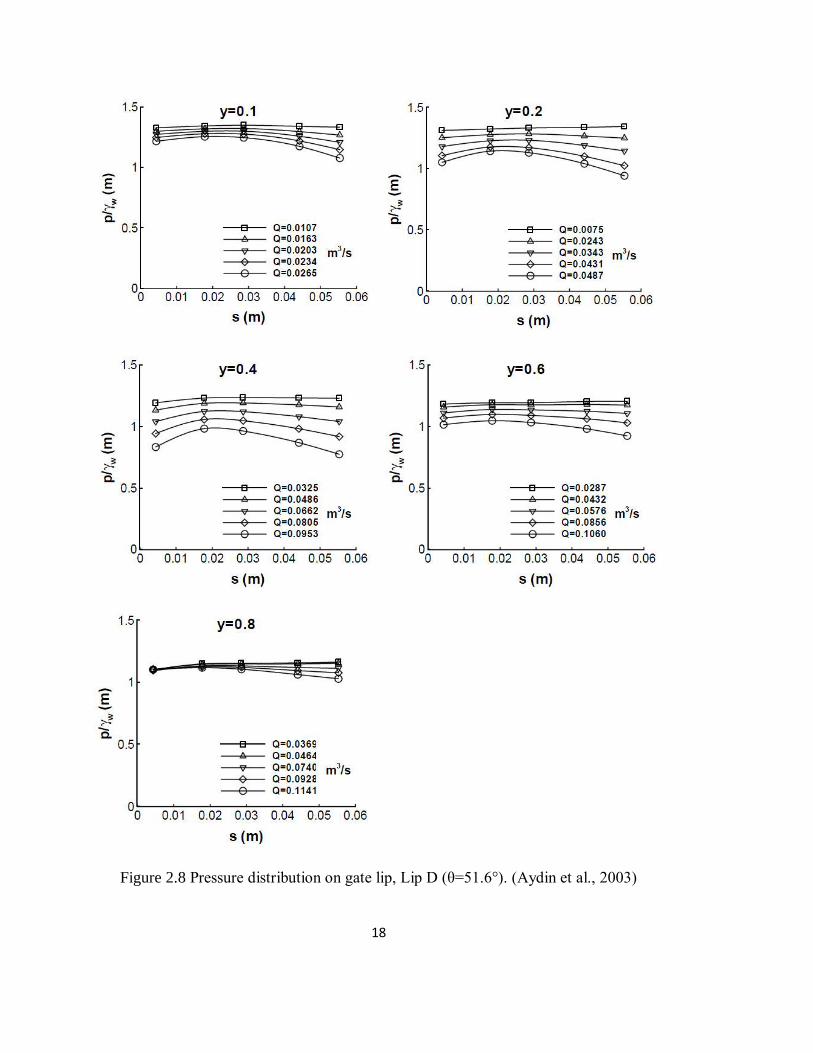
To investigate the variations of the downpull coefficient, five gate openings (y=0.1, 0.2,

0.4, 0.6, 0.8) and five different discharge values for each opening were experimented.

Pressure distributions on the gate lips were presented as a function of the distance s, along

the inclined gate lip face (in flow direction). Pressure distributions on four different gate

lips from experimental study are shown in Figures 2.5, 2.6, 2.7 and 2.8. Because of the

flow separation occurrence, it can be seen that the pressure near upstream edge is lower.

The data points shown in the figures are representing the piezometric readings taken from

the holes located on the demountable gate lip. Therefore, it should be said that the graphics

are based upon five data points only.

During the hydraulic study, the water level in the reservoir was greatly affected by the

fluctuations, consequently was subjected to small changes, thus it was difficult to maintain

the water level. Therefore it should be noted that the reservoir water level in each

experiment which the results are given through Figures 2.5 to 2.8 are not the same.

15

Figure 2.5 Pressure distribution on gate lip, Lip A (θ=26.5°). (Aydin et al., 2003)

16

Figure 2.6 Pressure distribution on gate lip, Lip B (θ=36.7°). (Aydin et al., 2003)

17

Figure 2.7 Pressure distribution on gate lip, Lip C (θ=44.7°). (Aydin et al., 2003)

18

Figure 2.8 Pressure distribution on gate lip, Lip D (θ=51.6°). (Aydin et al., 2003)

19

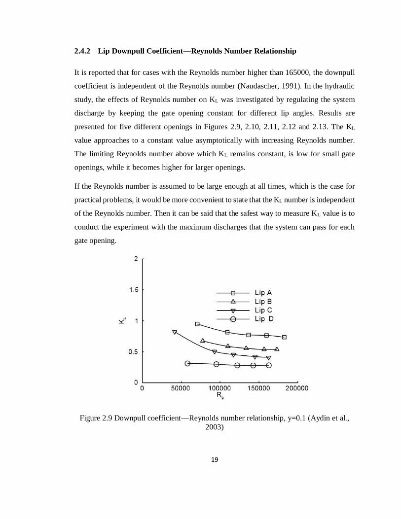
2.4.2 Lip Downpull Coefficient—Reynolds Number Relationship

It is reported that for cases with the Reynolds number higher than 165000, the downpull

coefficient is independent of the Reynolds number (Naudascher, 1991). In the hydraulic

study, the effects of Reynolds number on KL was investigated by regulating the system

discharge by keeping the gate opening constant for different lip angles. Results are

presented for five different openings in Figures 2.9, 2.10, 2.11, 2.12 and 2.13. The KL

value approaches to a constant value asymptotically with increasing Reynolds number.

The limiting Reynolds number above which KL remains constant, is low for small gate

openings, while it becomes higher for larger openings.

If the Reynolds number is assumed to be large enough at all times, which is the case for

practical problems, it would be more convenient to state that the KL number is independent

of the Reynolds number. Then it can be said that the safest way to measure KL value is to

conduct the experiment with the maximum discharges that the system can pass for each

gate opening.

Figure 2.9 Downpull coefficient—Reynolds number relationship, y=0.1 (Aydin et al.,

2003)

20

Figure 2.10 Downpull coefficient—Reynolds number relationship, y=0.2 (Aydin et al.,

2003)

Figure 2.11 Downpull coefficient—Reynolds number relationship, y=0.4 (Aydin et al.,

2003)

21

Figure 2.12 Downpull coefficient—Reynolds number relationship, y=0.6 (Aydin et al.,

2003)

Figure 2.13 Downpull coefficient—Reynolds number relationship, y=0.8 (Aydin et al.,

2003)

22

2.4.3 Lip Downpull Coefficient as a Function of the Gate Opening and the Lip

Angle

One of the most important outcome of this experimental study is the KL coefficient. This

coefficient was presented as function of two dimensionless variable, which are lip angle,

θ, and the dimensionless gate opening, y, in Figure 2.14.

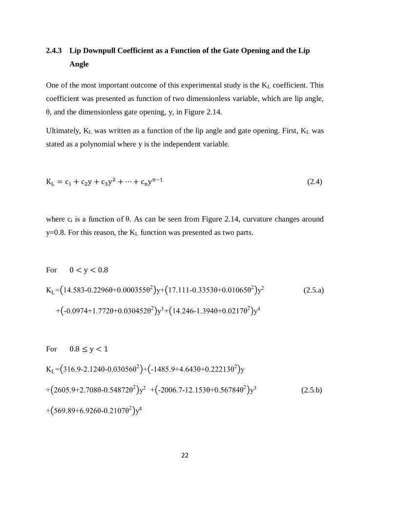
Ultimately, KL was written as a function of the lip angle and gate opening. First, KL was

stated as a polynomial where y is the independent variable.

KL = c1 + c2y + c3y2 + ⋯ + cnyn−1 (2.4)

where ci is a function of θ. As can be seen from Figure 2.14, curvature changes around

y=0.8. For this reason, the KL function was presented as two parts.

For 0 < y < 0.8

KL=(14.583-0.2296θ+0.000355θ2)y+(17.111-0.3353θ+0.01065θ

2)y2 (2.5.a)

+(-0.0974+1.772θ+0.030452θ2)y3+(14.246-1.394θ+0.0217θ

2)y4

For 0.8 ≤ y < 1

KL=(316.9-2.124θ-0.03056θ2)+(-1485.9+4.643θ+0.22213θ

2)y

+(2605.9+2.708θ-0.54872θ2)y2 +(-2006.7-12.153θ+0.56784θ

2)y3 (2.5.b)

+(569.89+6.926θ-0.2107θ2)y4

23

Equation 2.5 is valid for lip angles larger than 26° and smaller than 52° at every gate

opening (0<y<1). Downpull coefficient can be calculated from Equation 2.5 and then the

downpull force on the gate lip can be evaluated.

Figure 2.14 Downpull coefficient as a function of gate opening and gate lip angle (Aydin

et al., 2003)

24

25

CHAPTER 3

COMPUTATIONAL MODEL

GAMBIT v2.4.6 is used for forming the geometry and mesh generation. For simulations,

ANSYS FLUENT v14.0 is used as the solver, pre and post processor. The scale of the

computational model is selected to be the same as the experimental study.

3.1 Mesh Generation with GAMBIT

GAMBIT is a geometry and mesh generation software package designed to help analysts

and designers build and mesh the models for computational fluid dynamics (CFD) and

other scientific applications, usually used with FLUENT. GAMBIT's single interface for

geometry creation and meshing brings together most of FLUENT's preprocessing

technologies in one environment.

3.1.1 Forming the Geometry

The general geometry is adapted from the aforementioned experiment. Unlike the full

three dimensional experimental model, the system is modelled in 2D. The full domain and

final form of the geometry can be seen in Figure 3.1.

The geometry is adapted without the following features;

26

1. The ventilation chamber is not modelled and is not taken into account. It will be

seen later in this thesis that the results are not affected by the presence of the air

chamber.

2. Tail water region is not modelled as it was done in the experiment. Details of

downstream geometry of the pipe, such as its length, is not specified in the

numerical model, since the experiment has its own structure for regulating the flow

and a tank where the tail water is accumulated. Since it is hard to define such

structure, the region, namely the pipe after the gate, representing the downstream

of the gate is kept long enough in the numerical model to avoid any backflow

issues.

3. Intake is also modelled in a different way. Since it is needed to obtain a fully

developed flow before the gate, an intake structure was built in this experiment as

shown in Figure 2.2. However, in this computational study, for the sake of an easy

modelling, the intake region is modelled as a straight rectangular duct, and this

region is kept long enough for the flow to reach its fully developed state. The

upstream region can be defined as the pipe starting from inlet, reaches up to the

gate area. The length of the upstream region, along with the downstream length,

are decided by numerical experiments and will be discussed later in the thesis.

27

Fig

ure

3.1

Geo

met

ry f

orm

ed b

y G

AM

BIT

28

3.1.2 Forming the Grid

As it can be seen from the Figure 3.2, the geometry is generated using block-based

modelling. This type of modelling is helpful while forming the mesh, as one can control

the number of grid points and the grid size along the boundaries of these blocks.

Figure 3.2 Block based modelling

The reason for using block based modelling for the domain can be explained by two

elements;

- Since finer grid resolution is required close to the solid boundaries and the grid

elements get coarser as it approaches the center of the duct and away from the gate,

it is needed to do clustering. The clustering process is not carried out by a uniform

ratio, so blocking was considered as an option to control this element enlargement

process.

- In case of a need of a re-mesh of a specific part of the model, the block can be re-

meshed without the need of changing the non-related mesh in a further area. It is

also a time consuming process to re-mesh all the domain once the model is

changed. Block based modelling helps for this reason.

29

3.1.3 Clustering

Clustering, also known as grading or refinement can be defined as assigning a progressive

spacing between grid points, to change how accurately the solution is wanted to be

calculated in that region.

Mesh is refined near walls and clustered by blocks as it gets far away from the walls up to

some level as seen in Figure 3.3. Close to the solid walls a structured mesh is used along

a small band parallel to the side walls. Then, an unstructured grid is used towards the

center of the duct until the coarsening of the mesh is sufficient. A structured mesh is used

once again through a large band along the center. Refinement or coarsening are done

considering a smooth transition from walls to the center area.

This mesh refinement has been done in all models, in order to gather accurate results near

essential areas such as near walls and around the gate and especially gate lip. Since it is

desired to obtain the whole mesh with grid points as few as possible, some areas are

considered to be less important than these essential areas.

As can be seen from the Figure 3.3, quadrilateral elements are used for meshing. By

examining the mesh it can be seen that the quadrilateral mesh has lower skewness which

improves quality and convergence rate of the solution. It also gives better control of the

mesh, especially near walls.

30

Figure 3.3 Mesh refinement

Since more detailed data with less error is desired from gate lip calculations, the area

around the gate lip is meshed finer than the rest of the domain as shown in Figure 3.4.

After completion of meshing of each block, the generated mesh is checked for the quality.

The reason behind this check is because properties such as skewness can greatly affect the

accuracy and robustness of the CFD solution.

It is not practical to show the complete domain in the thesis. Therefore mesh around the

gate, part of the upstream and the transition of the mesh at downstream are shown in Figure

3.5.

31

Figure 3.4 Mesh around the gate

Figure 3.5 Mesh around gate and parts of upstream and downstream

3.1.4 Near Wall Mesh

In order to calculate the shear stresses and velocity profiles near wall precisely, structured

mesh is generated near walls, where the grid lines are perpendicular to the walls.

The geometry is modelled considering the near wall treatment. The mesh is stretched near

the walls so that the first grid point always falls inside the viscous sublayer.

32

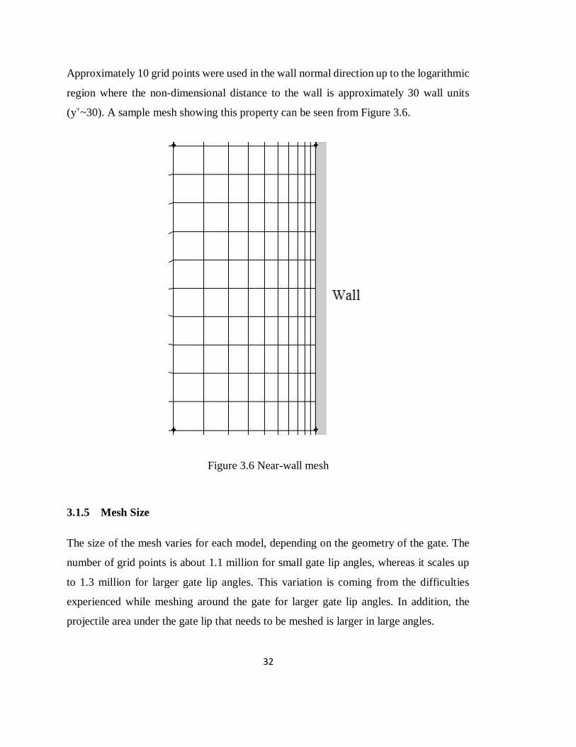
Approximately 10 grid points were used in the wall normal direction up to the logarithmic

region where the non-dimensional distance to the wall is approximately 30 wall units

(y+~30). A sample mesh showing this property can be seen from Figure 3.6.

Figure 3.6 Near-wall mesh

3.1.5 Mesh Size

The size of the mesh varies for each model, depending on the geometry of the gate. The

number of grid points is about 1.1 million for small gate lip angles, whereas it scales up

to 1.3 million for larger gate lip angles. This variation is coming from the difficulties

experienced while meshing around the gate for larger gate lip angles. In addition, the

projectile area under the gate lip that needs to be meshed is larger in large angles.

33

3.1.6 Boundary Conditions

The inlet section of the model is defined as “Velocity Inlet” and the outlet section is

defined as the “Pressure Outlet”. All boundaries, including the gate except inlet and outlet

are defined as “Wall” in GAMBIT. More information about the boundary conditions are

explained in the following sections.

3.2 ANSYS FLUENT Setup and Simulations

For simulations, ANSYS FLUENT is used. FLUENT is a state-of-the-art computer

program, written in C programming language for modeling fluid flow in complex

geometries and a variety of applications.

The mesh is transferred from GAMBIT. The procedure for a typical simulation is shown

step by step in the following sections.

3.2.1 Importing the Mesh

The mesh imported from GAMBIT to FLUENT. FLUENT automatically recognizes the

mesh and the boundary conditions, as these software are compatible with each other.

3.2.2 Scaling, Defining the Material and Gravity

Before being used, the system is scaled by an integrated scale function, since all GAMBIT

models are generated using centimeters, whereas meter is used as the length unit in

FLUENT. After that, water is defined as the material in the pipe and the zone is set to be

all water. Water is defined from the integrated database of FLUENT and the properties

are shown in Table 3.1.

34

Table 3.1 Material definition

Material Density Viscosity

water-liquid (h2o<l>) 998.2 kg/m3 0.001003 kg/m·s

The operating pressure of the system is set to be atmospheric pressure, which is 101325

Pascal, since the system is open to the atmosphere from the outlet. The gravity is set as

9.81 m/s2 acting in –y direction. It should be noted here that whether the model is solved

with or without gravity calculations, entering gravitational acceleration coefficient has a

negligible effect on the general solution of the problem.

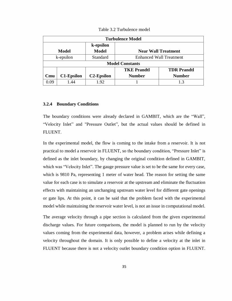
3.2.3 Turbulence Model

For turbulence modelling, k-epsilon turbulence model is used with the option “Enhanced

Wall Treatment”, because, as mentioned, near wall treatment is considered while

generating the computational grid. Enhanced wall treatment is a near-wall modeling

method that combines a two-layer model with enhanced wall functions. This option

requires that the mesh is to be fine enough near walls, to resolve the laminar sublayer.

Default option, which is the standard wall function is applicable in geometries meshed

with no near wall considerations. However it is not considered to be an advisable option,

since the degree of fineness, particularly near walls, is important especially in complex

geometries with high Reynolds numbers. Inputs for turbulence modelling is given in Table

3.2.

35

Table 3.2 Turbulence model

Turbulence Model

Model

k-epsilon

Model Near Wall Treatment

k-epsilon Standard Enhanced Wall Treatment

Model Constants

Cmu C1-Epsilon C2-Epsilon

TKE Prandtl

Number

TDR Prandtl

Number

0.09 1.44 1.92 1 1.3

3.2.4 Boundary Conditions

The boundary conditions were already declared in GAMBIT, which are the “Wall”,

“Velocity Inlet” and "Pressure Outlet”, but the actual values should be defined in

FLUENT.

In the experimental model, the flow is coming to the intake from a reservoir. It is not

practical to model a reservoir in FLUENT, so the boundary condition, “Pressure Inlet” is

defined as the inlet boundary, by changing the original condition defined in GAMBIT,

which was “Velocity Inlet”. The gauge pressure value is set to be the same for every case,

which is 9810 Pa, representing 1 meter of water head. The reason for setting the same

value for each case is to simulate a reservoir at the upstream and eliminate the fluctuation

effects with maintaining an unchanging upstream water level for different gate openings

or gate lips. At this point, it can be said that the problem faced with the experimental

model while maintaining the reservoir water level, is not an issue in computational model.

The average velocity through a pipe section is calculated from the given experimental

discharge values. For future comparisons, the model is planned to run by the velocity

values coming from the experimental data, however, a problem arises while defining a

velocity throughout the domain. It is only possible to define a velocity at the inlet in

FLUENT because there is not a velocity outlet boundary condition option in FLUENT.

36

This problem is solved by defining a boundary condition “Velocity Inlet” at the outlet of

the domain and entering the velocity value as negative, again by changing the original

condition defined in GAMBIT, which was “Pressure Outlet”. This process forces the

FLUENT to maintain the desired flow rate throughout entire domain.

Rest of the boundaries are left as “Wall”. Even if these boundaries was not defined,

FLUENT automatically detects that these locations should be set as a wall. Yet, all walls

were labeled differently for easy extraction of values, such as gate lip, which is named

separately and extracted to find pressure values isolated from its surroundings. Walls are

defined as stationary walls with no slip shear condition with the default wall roughness

coefficients which are given in Table 3.3.

Table 3.3 Wall roughness properties

Wall Roughness

Roughness Height (m) 0

Roughness Constant 0.5

3.2.5 Residuals

As the code iterates, "residuals" are calculated for each flow equation. These residuals

represent a kind of average error in the solution – if a predefined maximum residual is set

to be smaller, convergence takes more time. FLUENT checks five different convergence

residuals on each step of this iterative process. These residuals are for continuity, x-

velocity, y velocity, k and epsilon. The maximum residual criteria value is set to 10-6. This

value is tested to be sufficient to achieve a converged solution.

After scaling, setting gravity, the type of turbulence model, defining the material, setting

zone conditions, residuals, and boundary conditions, the system is initialized from the

outlet for faster convergence, the average velocity magnitude is set initially throughout

37

the whole flow domain. After initializing the setup, the simulation is run until desired

residuals are reached.

3.2.6 Simulations

The simulations carried out for each case until the desired residuals have been reached.

The average run time of a single model to reach that residuals, varies between 3 to 6 hours

with a computer with configurations given in Table 3.4.

Table 3.4 System configurations

Processor 1.6 GHz Intel Core i7 720QM

Memory 6GB, 1066 MHz DDR3

Chipset Intel HM55

Iteration count and simulation time depends on the gate opening and the discharge. For

smaller openings, the run time takes longer compared to the larger opening of gates. For

example, for y=0.2 opening model, where y is the ratio of the gate opening to the height

of the gate, the iteration count is around 7000 to reach the maximum residual, where in

y=0.4 it is around 5000. A typical iteration vs. residual count is shown in Figure 3.7. It is

seen that residuals experiences a quick drop at the beginning of the iterations, then they

continue to drop until all of the residuals reach or pass below the desired maximum

residual value. Once all residual criterion is achieved for all of the five residuals, the

simulation is stopped and the model becomes ready for post-processing.

For some selected models, simulation is run for further 1000 iterations for investigating if

further iterations has any effects on the solution. It is found out that the effects of further

iterations are negligible after reaching the predefined residual of 10-6.

38

Figure 3.7 Residuals

3.3 Selecting the Domain Size

The downstream and upstream part of the system can be defined as the domain part before

the gate and after the gate, respectively. It is noted that the downstream part should be

long enough to overcome backflow issues, and the upstream should be long enough to

develop a fully developed velocity profile. The length of these parts are decided by trial

and error. The system is modelled and solved for different lengths of these parts and then

a model size is selected and the rest of the simulations are carried out using that length.

The main purpose of these trials is to have a mesh of small size as much as possible.

Calculation time is significantly decreased if a smaller mesh size is used.

Trials are carried out using different lengths for the upstream and the downstream part.

The trials are started from 6 times duct height upstream and 16 times duct height

downstream, where the duct height is 30 cm, and the domain is meshed accordingly. The

upstream part is elongated by increments of 2 duct heights (2e0), while keeping the length

of the downstream part constant. These tests are done for two different gate openings with

maximum discharge that they can pass. The trials done for selecting the length of the

39

upstream for two gate openings and discharges are given in Table 3.5. The same procedure

is done for the downstream part. The downstream part is also elongated by 2e0 increments,

but this time keeping the length of the upstream part constant. Tests for selecting the length

of the upstream are done for the same two different gate openings with maximum

discharge that they can pass. The trials done for selecting the length of the downstream

for two gate openings and discharges are given in Table 3.6.

After simulations carried out by FLUENT, results are compared. After comparing the KL

values, 10e0 and 12e0 is decided to be the most suitable length at the upstream and

downstream, respectively.

Table 3.5 Variation in KL for different upstream lengths

Case y=0.2, θ=44.7°, Q=0.0496 m3/s y=0.4, θ=44.7°, Q=0.0955 m3/s

Lengths (u/s-d/s) 6e0-16e0 8e0-16e0 10e0-16e0 6e0-16e0 8e0-16e0 10e0-16e0

KL 0.63204 0.62719 0.62396 0.76721 0.76262 0.75975

% deviation 0.77192 0.51874 0.60068 0.37899

Table 3.6 Variation in KL for different downstream lengths

Case y=0.2, θ=44.7°, Q=0.0496 m3/s y=0.4, θ=44.7°, Q=0.0955 m3/s

Lengths

(u/s-d/s)

10e0-

12e0

10e0-

14e0

10e0-

16e0

10e0-

18e0

10e0-

12e0

10e0-

14e0

10e0-

16e0

10e0-

18e0

KL 0.62396 0.62396 0.62396 0.62396 0.75973 0.75974 0.75975 0.75975

%

deviation

0.00004 0.00004 0.00002

0.00048 0.00052 0.00053

40

The reason for selecting 10e0 and 12e0 lengths can be seen by looking at the error

percentages which are getting smaller as an optimum mesh is reached. After selecting 10e0

and 12e0 lengths, all the simulations are carried out using these lengths.

3.4 Grid Dependence Study

For investigating the effects of the grid size on the solution, a sample GAMBIT model is

re-meshed with two different meshes by lowering and increasing the size of the grid. Then,

these models are solved by FLUENT and the KL value is compared.

Lip angle θ=44.7° (Lip C) with y=0.4 gate opening is selected as the geometry to be used

in the grid dependence study. The selected model has 1265568 grid points before

modification. The mesh is lowered to 827598 grid points, where the percentage of

decrease is about 35%. Mesh increase is done to the same model by increasing the grid

points to 1625707, with the percentage about 28%. Largest possible discharge value for

the opening is selected for the simulations, which is 0.0955 m3/s.

The comparison of KL values and the number of grid points for these two models are given

in Table 3.7.

It is seen that lowering the mesh size by 34.6%, ends up with a 4.96% change in the KL

value and increasing the mesh size by 28.5%, ends up with a 0.22% change in KL value.

The change in the value obtained from lowering the mesh size, can be seen as an error

percentage which may likely alter the solution or gives incorrect results. By increasing the

mesh, it is seen that the change in the KL value is too small and can be considered as

insignificant.

Therefore, throughout this thesis, all models are generated using the mesh of Model 1.

41

Table 3.7 Grid points and KL comparison

Grid Points

Percentage relative to the

Original Model (Grid

size) KL

Percentage relative to

the Original Model (KL)

Model 1 1265568 0.7597

Model 2 827598 -34.61 0.7220 -4.96

Model 3 1625707 +28.46 0.7614 +0.22

3.5 Computational Results

3.5.1 Processing for Results

After simulations have been done, the static pressure on the gate lip is extracted from

FLUENT to a spreadsheet file. This file shows the static pressure on each node located on

the gate lip. After extracting this file, Equation 2.3, which is mentioned in the definition

of the downpull force coefficient is used to find head loss.

AhL, which is the projected area of each element along the gate lip, is found by subtracting

the neighbor x coordinates and taking their median whereas hp, the piezometric head is

found by dividing the static pressure to specific weight of water.

h2*, is defined as the piezometric head just upstream from the gate, that is the reservoir

head minus the entrance losses. Since the entrance losses have to be excluded for all the

cases investigated, an additional simulation without the gate is modelled and solved using

the same boundary conditions. The head losses due to friction coming from the presence

of the gate is eliminated by this type of approach. The static pressure value at the location

42

where the gate was used to be, is read from the FLUENT solutions and divided by specific

weight to find h2*.

Ug, which is the average velocity under the gate is also calculated from FLUENT for each

case. A vertical interface is defined at the desired location, which is the area under the

gate, and the average velocity is found by extracting area-weighted average.

hl̅ is calculated by integrating the piezometric head (denoted as static pressure over

specific weight in FLUENT) over the horizontally projected area of the gate lip. This

calculation is carried out for each grid point and corresponding projected element area and

the summation is made out using Microsoft Excel.

After revealing all unknowns, KL is calculated using Equation 2.2.

3.5.2 Computational Models

Compared to the experimental study, number of measured data points are much more in

the computational study, which gives an opportunity to monitor small changes of pressure

on the gate lip. Data is recorded for each grid point located on the gate lip, which starts

from the beginning of the curved part of the gate lip and ends at the tip of the lip. The

number of these grid points varies for each model but for the sake of a clear understanding,

it can be said that this number is about 700 on average.

The same experiments are modelled and simulated for the given discharges and gate

openings. In addition to the experimental gate openings that were simulated, nine more

gate openings (y=0.3, y=0.5, y=0.7, y=0.85, y=0.90, y=0.95, y=0.97, y=0.98, y=1.00) are

solved for a maximum discharge that the system can pass for each gate opening. These

discharges are selected from the proposed maximum discharge curve from the

experimental study. Maximum discharge is given as a function of gate opening in Figure

3.8, which is taken from the experimental study (Aydin et al., 2003).

43

Figure 3.8 Maximum system discharge (Aydin et al., 2003)

All model simulations which are done throughout this thesis are presented in Table 3.8

and Table 3.9. In addition to the ones summarized in these tables, additional simulations

are also carried out for the models without the presence of the gate. Therefore, the total

number of simulations done for this thesis is about 250.

44

Table 3.8 Simulations carried out (θ=26.5° and θ=36.7°)

Table 3.9 Simulations carried out (θ=44.7° and θ=51.6°)

y=0.10 0.0126 0.0184 0.0225 0.0260 0.0295 0.0136 0.0185 0.0221 0.0256 0.0280

y=0.20 0.0184 0.0313 0.0426 0.0485 0.0550 0.0212 0.0341 0.0440 0.0513 0.0573

y=0.30

y=0.40 0.0203 0.0384 0.0645 0.0723 0.0947 0.0286 0.0518 0.0711 0.0906 0.0997

y=0.50

y=0.60 0.0203 0.0402 0.0588 0.0795 0.1007 0.0382 0.0625 0.0823 0.1024 0.1182

y=0.70

y=0.80 0.0289 0.0455 0.0666 0.0850 0.1079 0.0421 0.0600 0.0831 0.1029 0.1211

y=0.85

y=0.90

y=0.95

y=0.97

y=0.98

y=1.00

0.0800

0.1107

0.1182

0.1220

0.1220

0.1219

0.1218

0.1216

0.1194

θ=26.5° θ=36.7°

Q (m3/s)

0.1107

0.1182

0.1194

0.1216

0.1218

0.0800

Gate

Opening

0.1219

0.1220

0.1220

y=0.10 0.0082 0.0159 0.0196 0.0238 0.0264 0.0011 0.0016 0.0203 0.0234 0.0265

y=0.20 0.0121 0.0267 0.0359 0.0441 0.0496 0.0075 0.0243 0.0343 0.043 0.049

y=0.30

y=0.40 0.028 0.053 0.069 0.082 0.096 0.033 0.049 0.066 0.081 0.095

y=0.50

y=0.60 0.0409 0.0605 0.0750 0.0899 0.1080 0.0287 0.0432 0.0576 0.0856 0.1060

y=0.70

y=0.80 0.0413 0.0606 0.0827 0.0985 0.1148 0.0369 0.0464 0.0740 0.0928 0.1141

y=0.85

y=0.90

y=0.95

y=0.97

y=0.98

y=1.00

Gate

Opening

Q (m3/s)

θ=44.7° θ=51.6°

0.1216

0.1218

0.0800

0.1107

0.1182

0.1194

0.1220

0.1220

0.1219

0.1220

0.1220

0.0800

0.1107

0.1182

0.1194

0.1216

0.1218

0.1219

45

3.5.3 Pressure Distributions on the Gate Lip

Pressure distributions on four different gate lips for five different gate openings at

different discharges from computational study are shown in Figures 3.9, 3.10, 3.11 and

3.12.

Since mesh size on the gate lip is very fine, there are approximately 700 data points where

all the flow quantities are recorded, remembering that in the experiments data is recorded

on only five points along the gate lip. Because of this, sudden changes on the pressure

along the gate lip can be captured within the simulations. Pressure values extracted from

FLUENT, which are shown in the figures, are “Static Pressure”, representing the

piezometric pressure.

It is seen that pressure on the gate lip experiences a sudden drop at the curved part of the

gate lip. This drop is more observable at gate openings y=0.2 and y=0.4. It can also be

said that, as the gate lip angle decreases, in other words, as the gate lip becomes more

parallel to the duct bottom, this pressure drop becomes more drastic as the flow

separations becomes more likely to occur as the gate lip becomes less streamlined. It is

also seen that another pressure drop occurs at the tip of the gate lip, as another flow

separation occurs at the tip. Unlike the previous observation, this pressure drop is more

noticeable for higher gate lip angles.

As it is mentioned in Chapter 2, the water level in the reservoir in experimental study is

not same for each model. However, in computational model, the upstream water level is

kept constant, which is 1 meter. Therefore, it is not possible to make a one to one

comparison for the pressure distributions of experimental study and computational study.

46

Figure 3.9 Pressure distribution on gate lip, Lip A (θ=26.5°). (Computational)

-0.5

0

0.5

1

1.5

0 0.02 0.04 0.06

p/γ

w(m

)

s (m)

y=0.1

Q=0.0126 m3/s Q=0.0184 m3/s

Q=0.0225 m3/s Q=0.0260 m3/s

Q=0.0295 m3/s

-0.5

0

0.5

1

1.5

0 0.02 0.04 0.06

p/γ

w(m

)

s (m)

y=0.2

Q=0.0184 m3/s Q=0.0313 m3/s

Q=0.0426 m3/s Q=0.0485 m3/s

Q=0.0550 m3/s

-0.5

0

0.5

1

1.5

0 0.02 0.04 0.06

p/γ

w(m

)

s (m)

y=0.4

Q=0.0203 m3/s Q=0.0384 m3/s

Q=0.0645 m3/s Q=0.0723 m3/s

Q=0.0947 m3/s

0

0.5

1

1.5

0 0.02 0.04 0.06

p/γ

w(m

)

s (m)

y=0.6

Q=0.0203 m3/s Q=0.0402 m3/s

Q=0.0588 m3/s Q=0.0795 m3/s

Q=0.1007 m3/s

0

0.5

1

1.5

0 0.02 0.04 0.06

p/γ

w(m

)

s (m)

y=0.8

Q=0.0289 m3/s Q=0.0455 m3/s

Q=0.0666 m3/s Q=0.0850 m3/s

Q=0.1079 m3/s

47

Figure 3.10 Pressure distribution on gate lip, Lip B (θ=36.7°). (Computational)

-0.5

0

0.5

1

1.5

0 0.02 0.04 0.06

p/γ

w(m

)

s (m)

y=0.1

Q=0.0136 m3/s Q=0.0185 m3/s

Q=0.0221 m3/s Q=0.0256 m3/s

Q=0.0280 m3/s

-0.5

0

0.5

1

1.5

0 0.02 0.04 0.06

p/γ

w(m

)

s (m)

y=0.2

Q=0.0212 m3/s Q=0.0341 m3/s

Q=0.0440 m3/s Q=0.0513 m3/s

Q=0.0573 m3/s

-0.5

0

0.5

1

1.5

0 0.02 0.04 0.06

p/γ

w(m

)

s (m)

y=0.4

Q=0.0286 m3/s Q=0.0518 m3/s

Q=0.0711 m3/s Q=0.0906 m3/s

Q=0.0997 m3/s

0

0.5

1

1.5

0 0.02 0.04 0.06

p/γ

w(m

)

s (m)

y=0.6

Q=0.0382 m3/s Q=0.0625 m3/s

Q=0.0823 m3/s Q=0.1024 m3/s

Q=0.1182 m3/s

0

0.5

1

1.5

0 0.02 0.04 0.06

p/γ

w(m

)

s (m)

y=0.8

Q=0.0421 m3/s Q=0.0600 m3/s

Q=0.0831 m3/s Q=0.1029 m3/s

Q=0.1211 m3/s

48

Figure 3.11 Pressure distribution on gate lip, Lip C (θ=44.7°). (Computational)

-0.5

0

0.5

1

1.5

0 0.02 0.04 0.06 0.08

p/γ

w(m

)

s (m)

y=0.1

Q=0.0082 m3/s Q=0.0159 m3/s

Q=0.0196 m3/s Q=0.0238 m3/s

Q=0.0264 m3/s

-0.5

0

0.5

1

1.5

0 0.02 0.04 0.06 0.08

p/γ

w(m

)

s (m)

y=0.2

Q=0.0121 m3/s Q=0.0267 m3/s

Q=0.0359 m3/s Q=0.0441 m3/s

Q=0.0496 m3/s

-0.5

0

0.5

1

1.5

0 0.02 0.04 0.06 0.08

p/γ

w(m

)

s (m)

y=0.4

Q=0.0283 m3/s Q=0.0533 m3/s

Q=0.0691 m3/s Q=0.0824 m3/s

Q=0.0955 m3/s

0

0.5

1

1.5

0 0.02 0.04 0.06 0.08

p/γ

w(m

)

s (m)

y=0.6

Q=0.0409 m3/s Q=0.0605 m3/s

Q=0.0750 m3/s Q=0.0899 m3/s

Q=0.1080 m3/s

0

0.5

1

1.5

0 0.02 0.04 0.06 0.08

p/γ

w(m

)

s (m)

y=0.8

Q=0.0413 m3/s Q=0.0606 m3/s

Q=0.0827 m3/s Q=0.0985 m3/s

Q=0.1148 m3/s

49

Figure 3.12 Pressure distribution on gate lip, Lip D (θ=51.6°). (Computational)

-0.5

0

0.5

1

1.5

0 0.02 0.04 0.06 0.08

p/γ

w(m

)

s (m)

y=0.1

Q=0.0107 m3/s Q=0.0163 m3/s

Q=0.0203 m3/s Q=0.0234 m3/s

Q=0.0265 m3/s

-0.5

0

0.5

1

1.5

0 0.02 0.04 0.06 0.08

p/γ

w(m

)

s (m)

y=0.2

Q=0.0075 m3/s Q=0.0243 m3/s

Q=0.0343 m3/s Q=0.0431 m3/s

Q=0.0487 m3/s

-0.5

0

0.5

1

1.5

0 0.02 0.04 0.06 0.08

p/γ

w(m

)

s (m)

y=0.4

Q=0.0325 m3/s Q=0.0486 m3/s

Q=0.0662 m3/s Q=0.0805 m3/s

Q=0.0953 m3/s

0

0.5

1

1.5

0 0.02 0.04 0.06 0.08

p/γ

w(m

)

s (m)

y=0.6

Q=0.0287 m3/s Q=0.0432 m3/s

Q=0.0576 m3/s Q=0.0856 m3/s

Q=0.1060 m3/s

0

0.5

1

1.5

0 0.02 0.04 0.06 0.08

p/γ

w(m

)

s (m)

y=0.8

Q=0.0369 m3/s Q=0.0464 m3/s

Q=0.0740 m3/s Q=0.0928 m3/s

Q=0.1141 m3/s

50

3.5.4 Lip Downpull Coefficient—Reynolds Number Relationship

Variation of lip downpull coefficient, KL, with Reynolds number for different lip

geometries is obtained from the simulation results and is presented for four different lip

angles through Figures 3.13 to 3.17. As it can be seen from these figures, KL is always

independent of the Reynolds number. Remember that in the experimental study KL was

independent from Reynolds number only for Re>1650000. Flow may have a transitional

behavior for low Reynolds numbers and k-epsilon (k-ε for short) turbulence model may

not be able to represent this. This may also be related to a steady 2D assumption made in

the simulations. It should also be noted that in practical problems the Reynolds numbers

encountered are much larger.

Figure 3.13 Downpull coefficient—Reynolds number relationship, y=0.1

(Computational)

0

0.1

0.2

0.3

0.4

0.5

0.6

0.7

0.8

0 5 0 0 0 0 1 0 0 0 0 0 1 5 0 0 0 0 2 0 0 0 0 0 2 5 0 0 0 0

KL

RG

Lip A

Lip B

Lip C

Lip D

51

Figure 3.14 Downpull coefficient—Reynolds number relationship, y=0.2

(Computational)

Figure 3.15 Downpull coefficient—Reynolds number relationship, y=0.4

(Computational)

0

0.2

0.4

0.6

0.8

1

1.2

0 1 0 0 0 0 0 2 0 0 0 0 0 3 0 0 0 0 0 4 0 0 0 0 0 5 0 0 0 0 0

KL

RG

Lip A

Lip B

Lip C

Lip D

0

0.2

0.4

0.6

0.8

1

1.2

1.4

0 1 0 0 0 0 0 2 0 0 0 0 0 3 0 0 0 0 0 4 0 0 0 0 0 5 0 0 0 0 0 6 0 0 0 0 0

KL

RG

Lip A

Lip B

Lip C

Lip D

52

Figure 3.16 Downpull coefficient—Reynolds number relationship, y=0.6

(Computational)

Figure 3.17 Downpull coefficient—Reynolds number relationship, y=0.8

(Computational)

0

0.2

0.4

0.6

0.8

1

1.2

0 1 0 0 0 0 0 2 0 0 0 0 0 3 0 0 0 0 0 4 0 0 0 0 0 5 0 0 0 0 0 6 0 0 0 0 0

KL

RG

Lip A

Lip B

Lip C

Lip D

-0.2

-0.1

0

0.1

0.2

0.3

0.4

0.5

0 1 0 0 0 0 0 2 0 0 0 0 0 3 0 0 0 0 0 4 0 0 0 0 0 5 0 0 0 0 0 6 0 0 0 0 0

KL

RG

Lip A

Lip B

Lip C

Lip D

53

3.6 Comparison of Selected Flow Properties

Three different properties, which are velocity magnitude, streamlines and turbulent kinetic

energy are selected to be graphically presented and compared for selected cases. Velocity

profiles under the gate lip section are also given. The case selection is made to show

variations in critical models.

First, to investigate the effects of gate opening, lip angle is kept constant and the gate

opening is changed for a maximum discharge that can pass for that gate opening. θ=26.5°

is selected to be the lip angle to be kept constant. Three gate openings are selected for a

constant lip angle, which are y=0.1, y=0.5 and y=0.9.

Then, lip angle is changed for a fixed gate opening with a maximum discharge to show

how the lip angle influences the solution. 40% gate opening (y=0.4) is selected to be kept

constant and the solutions are compared for four different gate lips. Note that 40% is the

gate opening where KL value reaches its maximum value where sudden pressure changes

are observable.

Finally, lip angle and gate opening is kept constant while changing the discharge to

demonstrate the effects of discharge on a typical model. θ=51.6° and y=0.2 are selected

to be fixed while changing the discharge value.

3.6.1 Effect of Gate Opening

Changes in the flow for three different gate openings, which are y=0.1, y=0.5 and y=0.9

are investigated. Figure 3.18 shows the velocity magnitude at three different gate

openings, namely y=0.1, y=5 and y=0.9. It is seen that flow is accelerating under the gate

section where the maximum velocity magnitude observed at that section is getting smaller

as the gate opening increases. Most crucial values are occurring at the gate opening of

10% where the maximum velocity magnitude is around 4.89 m/s. Velocity magnitudes

remain to be larger close to the bottom of the gate at the downstream of the gate section.

54

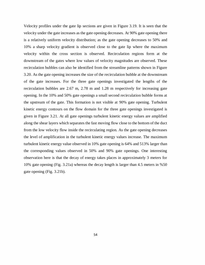
Velocity profiles under the gate lip sections are given in Figure 3.19. It is seen that the

velocity under the gate increases as the gate opening decreases. At 90% gate opening there

is a relatively uniform velocity distribution; as the gate opening decreases to 50% and

10% a sharp velocity gradient is observed close to the gate lip where the maximum

velocity within the cross section is observed. Recirculation regions form at the

downstream of the gates where low values of velocity magnitudes are observed. These

recirculation bubbles can also be identified from the streamline patterns shown in Figure

3.20. As the gate opening increases the size of the recirculation bubble at the downstream

of the gate increases. For the three gate openings investigated the lengths of the

recirculation bubbles are 2.67 m, 2.78 m and 1.28 m respectively for increasing gate

opening. In the 10% and 50% gate openings a small second recirculation bubble forms at

the upstream of the gate. This formation is not visible at 90% gate opening. Turbulent

kinetic energy contours on the flow domain for the three gate openings investigated is

given in Figure 3.21. At all gate openings turbulent kinetic energy values are amplified

along the shear layers which separates the fast moving flow close to the bottom of the duct

from the low velocity flow inside the recirculating region. As the gate opening decreases

the level of amplification in the turbulent kinetic energy values increase. The maximum

turbulent kinetic energy value observed in 10% gate opening is 64% and 513% larger than

the corresponding values observed in 50% and 90% gate openings. One interesting

observation here is that the decay of energy takes places in approximately 3 meters for

10% gate opening (Fig. 3.21a) whereas the decay length is larger than 4.5 meters in %50

gate opening (Fig. 3.21b).

55

Fig

ure

3.1

8 V

elo

cit

y m

agnit

ude

dis

trib

uti

on f

or

(A)

θ=

26.5

°, y

=0.1

, Q

=0.0

295 m

3/s

, (B

) θ=

26.5

°, y

=0.5

,

Q=

0.1

107 m

3/s

, (C

) θ=

26.5

°, y

=0.9

, Q

=0.1

216 m

3/s

(A)

(B)

(C)

56

Fig

ure

3.1

9 V

elo

cit

y p

rofi

les

under

the

gat

e se

ctio

n f

or

y=

0.1

, y=

0.5

and y

=0.9

57

Fig

ure

3.2

0 S

trea

mli

nes

for

(A)

θ=

26.5

°, y

=0.1

, Q

=0.0

295 m

3/s

, (B

) θ=

26.5

°, y

=0.5

, Q

=0.1

107 m

3/s

,

(C)

θ=

26.5

°, y

=0.9

, Q

=0.1

216 m

3/s

(A)

(B)

(C)

58

Fig

ure

3.2

1 T

urb

ule

nt

Kin

etic

Ener

gy f

or

(A)

θ=

26.5

°, y

=0.1

, Q

=0.0

295 m

3/s

, (B

) θ=

26.5

°, y

=0.5

,

Q=

0.1

107 m

3/s

, (C

) θ=

26.5

°, y

=0.9

, Q

=0.1

216 m

3/s

(A)

(B)

(C)

59

3.6.2 Effect of Lip Angle

Changes in the flow for four different lip angles, which are θ=26.5°, θ=36.7°, θ=44.7° and

θ=51.6°, are investigated. Velocity magnitude contours around the gate for the different

lip angles at 40% gate opening are given in Figure 3.22. Velocity magnitudes are amplified

beneath the gate for all the lip angles. However this amplification is largest at θ=51.6° and

smallest at θ=26.5°. Keeping in mind that discharge values are slightly different for the

four different gate lip angles and is largest for the lip angle of θ=36.7° one can say that

the amplification in the velocity magnitude increases as the gate lip angle increases. Figure

3.23 shows the velocity profiles under tip of the gate lip sections. It is seen that for large

lip angles (θ≥44.7°), the velocity reaches its maximum value at a very close distance to

the gate lip. Streamline patterns for the four lip angles investigated is given in Figure 3.24.

For all the lip angles two recirculation regions one at the upstream and one at the

downstream of the gate are present. As the lip angle increases the length of the

downstream recirculation region slightly increases. Figure 3.25 shows the turbulent

kinetic energy contours around the gate for the four different lip angles investigated. It

can be seen from this figure that as the gate lip angle increases the level of turbulence at

the downstream of the gate increases.

60

Fig

ure

3.2

2 V

elo

cit

y m

agnit

ude

dis

trib

uti

on f

or

(A)

θ=

26.5

°, y

=0.4

, Q

=0.0

947 m

3/s

, (B

) θ=

36.7

°,

y=

0.4

, Q

=0.0

997 m

3/s

, (C

) θ=

44.7

°, y

=0.4

, Q

=0.0

955 m

3/s

, (D

) θ=

51.6

°, y

=0.4

, Q

=0.0

953 m

3/s

(A)

(B)

(C)

(D)

61

Fig

ure

3.2

3 V

elo

cit

y p

rofi

les

under

the

gat

e se

ctio

n f

or

θ=

26.5

°, θ

=36.7

°, θ

=44.7

° an

d θ

=51.6

°

62

Fig

ure

3.2

4 S

trea

mli

nes

for

(A)

θ=

26.5

°, y

=0.4

, Q

=0.0

947 m

3/s

, (B

) θ=

36.7

°, y

=0.4

,

Q=

0.0

997 m

3/s

, (C

) θ=

44.7

°, y

=0.4

, Q

=0.0

955 m

3/s

, (D

) θ=

51

.6°,

y=

0.4

, Q

=0

.09

53 m

3/s

(A)

(B)

(C)

(D)

63

Fig

ure

3.2

5 T

urb

ule

nt

Kin

etic

Ener

gy f

or

(A)

θ=

26.5

°, y

=0.4

, Q

=0.0

947 m

3/s

, (B

) θ=

36.7

°, y

=0.4

,

Q=

0.0

997 m

3/s

, (C

) θ=

44.7

°, y

=0.4

, Q

=0.0

955

m3/s

, (D

) θ=

51

.6°,

y=

0.4

, Q

=0

.09

53 m

3/s

(A)

(B)

(C)

(D)

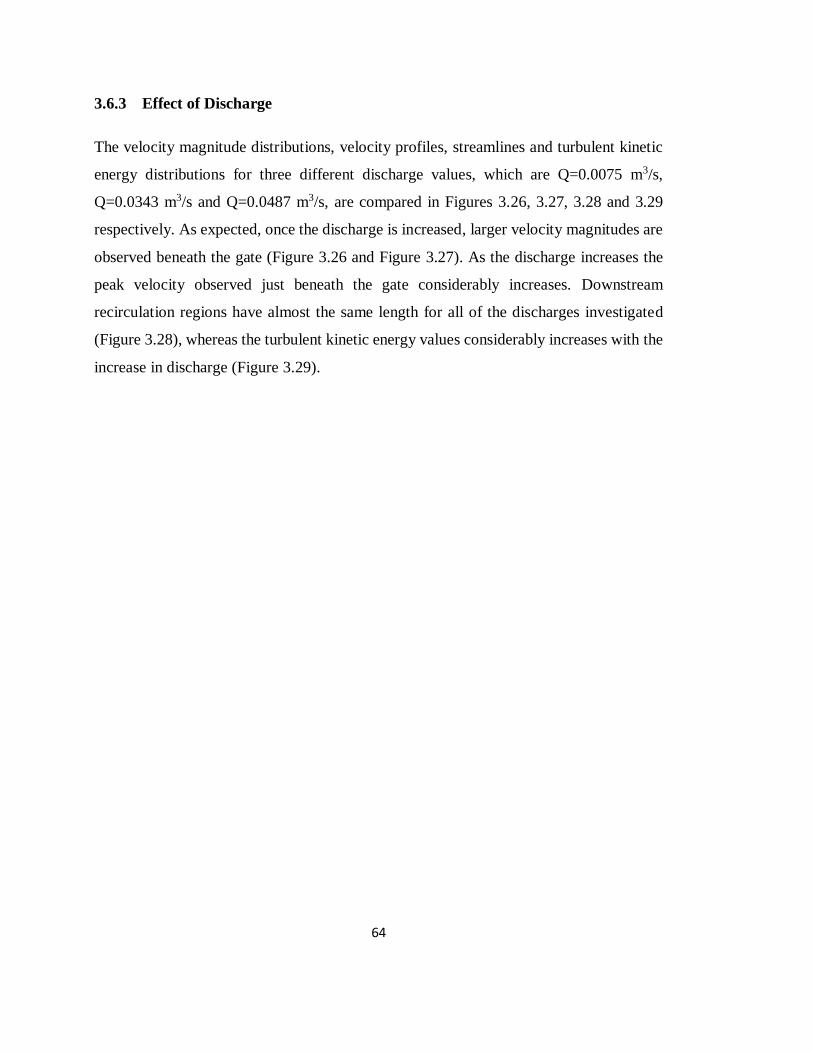
64

3.6.3 Effect of Discharge

The velocity magnitude distributions, velocity profiles, streamlines and turbulent kinetic

energy distributions for three different discharge values, which are Q=0.0075 m3/s,

Q=0.0343 m3/s and Q=0.0487 m3/s, are compared in Figures 3.26, 3.27, 3.28 and 3.29

respectively. As expected, once the discharge is increased, larger velocity magnitudes are

observed beneath the gate (Figure 3.26 and Figure 3.27). As the discharge increases the

peak velocity observed just beneath the gate considerably increases. Downstream

recirculation regions have almost the same length for all of the discharges investigated

(Figure 3.28), whereas the turbulent kinetic energy values considerably increases with the

increase in discharge (Figure 3.29).

65

Fig

ure

3.2

6 V

elo

cit

y m

agnit

ude

dis

trib

uti

on f

or

(A)

θ=

51.6

°, y

=0.2

, Q

=0.0

075 m

3/s

, (B

) θ=

51.6

°,

y=

0.2

, Q

=0.0

343 m

3/s

, (C

) θ=

51.6

°, y

=0.2

, Q

=0.0

487 m

3/s

(A)

(B)

(C)

66

Fig

ure

3.2

7 V

elo

cit

y p

rofi

les

under

the

gat

e se

ctio

n f

or

Q=

0.0

075 m

3/s

, Q

=0.0

343 m

3/s

and Q

=0.0

48

7 m

3/s

67

Fig

ure

3.2

8 S

trea

mli

nes

for

(A)

θ=

51.6

°, y

=0.2

, Q

=0.0

075 m

3/s

, (B

) θ=

51

.6°,

y=

0.2

, Q

=0

.03

43 m

3/s

,

(C)

θ=

51.6

°, y

=0.2

, Q

=0.0

487 m

3/s

(A)

(B)

(C)

68

Fig

ure

3.2

9 T

urb

ule

nt

Kin

etic

Ener

gy f

or

(A)

θ=

51.6

°, y

=0.2

, Q

=0.0

075 m

3/s

, (B

) θ=

51.6

°, y

=0.2

,

Q=

0.0

343 m

3/s

, (C

) θ=

51.6

°, y

=0.2

, Q

=0

.04

87 m

3/s

(A)

(B)

(C)

69

3.7 Lip Downpull Coefficient as a Function of the Gate Opening and the Lip

Angle

Figure 3.30 demonstrates downpull coefficient as a function of the gate lip angle and gate

opening, which is based on experimental study of Aydin et al. (2003). The details of this

study is given in Chapter 2.

Lip downpull coefficient, KL is zero at each side of the Figure 3.30, where the gate is fully

open (y=1) and fully closed (y=0). The reason for this is that at these two gate openings,

the piezometric head acting on the gate lip is equal to the piezometric head of the gate

section. It can be seen from the figure that the downpull coefficient is at its maximum

around 30-40% gate openings. The downpull coefficient is increasing with the decreasing

gate lip angle. Around 90% gate openings, the downpull coefficient is negative which

indicates that the piezometric head on the gate lip is larger than the piezometric head at

the gate section. In that case, an uplift occurs instead of a downpull.

As it is done in the experimental study, KL is stated as a polynomial where y is the

independent variable using data coming from computational results. The KL function will

also be presented as two parts, the same as the experimental study.

For 0 < y < 0.8

KL=(11-0.15532θ+0.00024897)y+(-12.429-0.092961θ+0.0043619θ2)y2 (3.1.a)

+(-13.521+1.1627θ-0.017538θ2)y3+(17.107-1.0551θ+0.01467θ

2)y4

For 0.8 ≤ y < 1

KL=(317.08-2.12203θ--0.030547θ2)+(-1485.1+4.6505θ+0.22251θ

2)y

+(2600.9+2.71θ-0.54836θ2)y2 +(-2004.1-12.128θ+0.56683θ

2)y3 (3.1.b)

+(570.65+6.93072θ-0.21095)y4

70

Because of the non-linearity of the y-KL curve, it is hard to obtain a generalized solution.

Coefficients of equation (2.5) are taken as initial guesses for the optimization of the

computational data. It should be noted that there is more than one solution for each of the

mentioned ranges, namely, 0<y<0.8 and 0.8≤y<1. Regardless of any similarities between

coefficients of equation (3.1) and (2.5), the equations obtained from computational study

give similar results to the experimental data.

Equation 3.1 is valid for 26°≤θ≤52°. Equation 3.1 will give the lip downpull coefficient,

KL, for given y and θ, and the downpull on the gate lip can be evaluated using this result.

Complete data set for the lip downpull coefficient, KL, evaluated using computed data of

this study are shown in Figure 3.30.

71

Fig

ure

3.3

0 D

ow

npu

ll c

oef

ficie

nt

as a

fu

nct

ion o

f th

e gat

e li

p a

ng

le a

nd

the

gat

e o

pen

ing (

Co

mputa

tio

nal)

72

3.8 Comparison of Experimental and Computational Values

Generally, two dimensional approach is an idealization to the three dimensional model. In

2D, for large Reynolds numbers, there is no turbulence due to absence of vortex tube

stretching in the third dimension. This prevents taking the effects of secondary flows into

account. These effects become more important for large openings, which have larger

velocity magnitudes, hence larger Reynolds numbers.

As it is mentioned in Chapter 2, the experimental model had a gate chamber, which is

absent for the computational model. For small gate openings, the momentum of the flow

and the pressure difference leads the water to flow over the gate, through the gate chamber,

causing leakage. Again, when the gate is fully closed, the experimental model might not

be able to prevent leakage, both through gate chamber and beneath the gate.

In preceding sections, downpull coefficient KL is presented as function of gate angle and

the gate opening, both for experimental and computational. In Figure 3.31, the KL values

coming from the computational study is sketched together with Equation 2.5, to see the

differences in dimensionless downpull coefficient, KL between experimental and

computational study.

Figure 3.31 shows that the computational KL values are matching with the Equation 2.5

where y is less than 0.8, except for Lip A, which is 26.5°. The computational KL values

for Lip A between y=0.3 and y=0.7 seem to be a little off from the experimental results.

However these values starts to get close to each other in range where y=0.8 and y=0.9,

where other values coming from other lip angles are apart from each other.

It is seen that after gate opening y=0.8, up to y=1.00, most computational KL values seem

to be far from experimental values. It should be noted here two gate openings (y=0.9333

and y=0.9666) used in the experiments conducted in hydraulic study, are not modeled in

computational study. Instead, three different gate openings, which are y=0.95, y=0.97 and

y=0.98 are used, considering that the KL values are more critical for gate openings close

73

to the fully opened gate. This may help the catch the behavior of the KL near y=1.00. In

Figure 3.31, between y=0.8 and y=1.00, experimental KL values are following a path away

from the axis, compared to the computational values which remain close to the axis.

Ultimately, both KL values at y=1.00 (where gate is fully opened) are zero or very close

to zero, therefore, if a curve is formed from the values of the computational study, it would

be more natural as it is following a smoother path (where there is no need for abrupt

changes of KL to reach 0 when y=1.00) compared to the experimental study.

74

Fig

ure

3.3

1 D

ow

npu

ll c

oef

ficie

nt

as a

fu

nct

ion o

f th

e gat

e li

p a

ng

le a

nd t

he

gat

e o

pen

ing

(Co

mputa

tio

nal and e

xper

imenta

l co

mp

aris

on)

75

CHAPTER 4

CONCLUSION

In this thesis, hydrodynamic downpull force is studied computationally on the created

models for variable gate openings and gate lip angles. Numerical models are generated to

represent the flow in a penstock or a tunnel and effects of this flow on a tunnel gate are

investigated.

It can be concluded that, for achieving the general accuracy of a CFD model, one should

consider the properties geometry, meshing, turbulence model and boundary conditions.

Domain size and the mesh generated for the simulations strongly affects the results.

The inflow and outflow sections should be selected at a sufficiently large distance

(10e0 and 12e0 for upstream and downstream, respectively) from the gate section

in order not to influence the results.

Grid independence check should be made in order to decide on the mesh size to

be used in the numerical study.

Grid refinement should be made at locations where large gradients on flow

quantities occur, or at locations where finer resolution is needed, i.e. because of

flow separation.

“Enhanced wall treatment” option in the turbulence model tab should be used for

flows which are massively separated, as for these flows logarithmic velocity

profile assumption is not valid.

76

The numerical simulations are efficient and less costly compared to the experimental

methods. However, it would be very beneficial to have at least one validation case from a

physical experiment. Yet, this thesis should be considered as a proof that CFD modelling

is a substitution to physical models.

FLUENT can be used with confidence in calculating the hydrodynamic downpull

coefficient KL for vertical high head gates, provided that the domain size, mesh size and

grid clustering is done correctly.

Steady, 2D flow assumptions are reasonable for the numerical simulations.

The range of applicability of findings of this study can be expanded by considering effects

of a moving gate on the downpull. In addition, results coming out from this study can also

be validated for a three dimensional model.

77

REFERENCES

Akoz, M. S., Kirkgoz, M. S., & Oner, A. A. (2009). Experimental and Numerical

Modeling of a Sluice Gate Flow. Journal of Hydraulic Research 47:2, 167-176.

Amorim, J. C., & Andrade, J. L. (1999). Numerical Analysis of the Hydraulic Downpull

on Vertical Lift Gates. Waterpower '99, 1-9.

Aydin, I. (2002). Air Demand Behind High Head Gates. Journal of Hydraulic Research

IAHR 40:1, 83-93.

Aydin, I., Dundar, O., & Telci, I. (2003). Hydrodynamic Loads on Closing Hydraulic

Gates (in Turkish). Ankara: METU.

Aydin, I., Telci, I., & Dundar, O. (2006). Prediction of Downpull on Closing High Head

Gates. Journal of Hydraulic Research IAHR 44:6, 822-831.

Dargahi, B. (2010). Flow Characteristics of Bottom Outlets with Moving Gates. Journal

of Hydraulic Research 48:4, 476-482.

Erbisti, P. C. (2004). Design of Hydraulic Gates. Tokyo: A.A Balkema Publishers.

Inc., A. (2011, November). ANSYS FLUENT User's Guide Release 14.0.

Inc., F. (2007, May). GAMBIT 2.4 Documentation.

Naudascher, E. (1986). Prediction and Control of Downpull on Tunnel Gates. Journal of

Hydraulic Engineering ASCE 112:5, 392-416.

Naudascher, E. (1991). Hydrodynamic Forces. Rotterdam: A.A. Balkema.

78

Naudascher, E., Kobus, H. E., & Rao, R. P. (1964). Hydrodynamic Analysis for High-

head Leaf Gates. Journal of the Hydraulics Division ASCE 90:3, 155-192.

Sagar, B. (1977). Downpull in High-head Gate Installations, Parts 1, 2, 3. Water Power

Dam Construct, (3), 38–39; (4), 52–55; (5), 29–35.

Sagar, B. (2000). Gate Lip Hydraulics. Water Power and Dam Construction.