prediction of 4340 steel hardness profile heat- treated by ... 4/issue 6/ijeit1412201412_03.pdf ·...
TRANSCRIPT

ISSN: 2277-3754
ISO 9001:2008 Certified International Journal of Engineering and Innovative Technology (IJEIT)
Volume 4, Issue 6, December 2014
14
Abstract— Laser hardening is one of the promising
manufacturing processes to enhance the materials mechanical
properties. Due to its capacity to heat locally and rapidly the
mechanical components, the process is able to produce reliable
parts able to challenge to wear and fatigue failures. However, it
is still difficult to predict the hardness profile using simulation or
experimental data since the process parameters and material
properties have a great effect on the process behavior. An
accurate prediction of the hardness profile heat-treated by laser
is a necessity to overcome the time consumption issue and
achieve best cost effective solution. The purpose of the present
study is to develop some approaches and compare them to
determine the hardness profile shape in relation with the laser
hardening parameters values range. The experimental data used
for modeling and validation were obtained based on systematic
tests according to Taguchi experimental design. Finally, artificial
neural network and mathematical based regression models are
built and confronted one to the other to converge towards the best
prediction model. The artificial neural network model is
distinguished by its high capability and good precision by
comparing the modeling and validation experimental data.
Keywords: Laser hardening; Hardness Profile; Experimental
data; Taguchi method; artificial neural network; nonlinear
regression.
I. INTRODUCTION
Surface hardening is very promising process applied to
low and medium-carbon steels to enhance wear resistance
and improve fatigue life. The surface hardening can be
performed using several techniques such as thermo
chemical, induction and laser processes. In fact, the laser
hardening process is more and more integrated in industries
since it permits to develop ultimate features mentioning
selective and local heating capacities, negligible distortion
and short cycle times. Secondly, it can be characterized by
its ability to improve the mechanical properties of the
materials by changing the superficial microstructure without
affecting greatly the core due to high temperature gradient
and high rate of its change. This combination of hard surface
and tough core is greatly desirable because it provides
favorable compressive stress distribution which reduces the
crack initiation and propagation processes [1]. Laser surface
hardening is considered by industrial to increase the
hardness and strength by quenching the material from the
austenite region to form hard marten site. Once the material
surface is heated by laser beam, the initial microstructure is
transformed to austenite in the regions heated above Ac3.
Thanks to the good harden ability of used steel (4340), the
austenitized layers are transformed to hard and fine
martensite forming the hardened region upon self-quenching
effect. An over-tempered region is noticed between the
hardened region and the material bulk which consist of
tempered martensite containing a small amount of retained
austenite. Emphasizing that high source of heat energy can
lead to melted region near the surface as shown in Figure 1
[2–3].
Fig 1. Schematic representation of regions produced by laser
hardening
The case depth that represents the hardened region depth
depends on the process parameters and material properties.
Therefore the process parameter value range should be
selected to ensure the complete austenitization of the steel
layer during the heat treatment. Over the past two decades,
laser hardening has experienced strong growth and because
of the growing number of applications, several studies are
performed with the aim to determine the optimal parameters
that affect the process outcome. As a result, the most
influential factors undisputed in laser hardening process are
the laser beam power and the scanning speed which can be
incorporated within the machine parameters category, that
affect strongly the interaction time of the laser radiation with
the hardened part of the component [4]. While other
parameters such the beam spot diameter, the focal length of
the laser, material absorption rate , the initial hardness and
the surface state of material can be considered minor
comparing to the two parameters mentioned above which
their influences varies from one to another [5]. The hardness
profile sensitivity can be defined as the behavior of outcome
variables in relation to process parameters levels. The case
depth (mm), the max and min hardness (HRC), the depth
and the hardness of the melted region are the usual outcome
variables with which the hardness profile regions can be
determined (Figure 2). Shiue and al [6] studied the effect of
Ilyes Maamri, Abderrazak El Ouafi and Noureddine Barka
Engineering Department, University of Quebec at Rimouski, QC, Canada
Prediction of 4340 Steel Hardness Profile Heat-
treated by Laser Using Artificial Neural
Networks and Multi Regression approaches

ISSN: 2277-3754
ISO 9001:2008 Certified International Journal of Engineering and Innovative Technology (IJEIT)
Volume 4, Issue 6, December 2014
15
the initial microstructure of AISI 4340 on hardness profile
behavior treated by CO2 laser; they mentioned that the
hardness curve can be generally divided into four regions,
such as the hardened zone, the over-tempered zone in which
the partial transformation occurred and the heat-unaffected
base metal. On the other hand, Purushothaman and al [7]
performed the laser hardening process using steel EN25 Nd:
YAG laser system, he denoted that the hardness profile
consist of three regions such as the hardened zone, the over-
tempered zone, and the heat-unaffected material core. He
denoted also that using the higher power densities, the
surface of the steel gets melted for all the travel speeds
which forming the melting zone.
Fig 2. Typical hardness curve
From literature survey, the few studies which have been
conducted with regard to the prediction of the laser
hardening process interest responses in relation with process
parameters levels were generally focused on the prediction
of the hardened layer dimension. As an experimental work,
Woo [8] estimated the hardened layer dimensions of SM45C
steel treated by 4 kW CO2 laser using special techniques for
prediction, such as the multi-regression model and the
artificial neural network model. He focused mainly on the
effect of the coating thickness on the hardened layer.
Shercliff and all [9] conducted a theoretical study that aims
the exploration of case depth prediction by developing an
approximate heat flow model. This model uses the laser
sources distribution such as Gaussian, rectangular and
uniform to exploit dimensional relationships between
process variables to provide ideal diagrams for the hardened
depth [9]. The literature reveals clearly the lack of works
that highlight the prediction of other hardness profile
outcomes. Based on the information related to the number of
the regions mentioned in references [6-7], and the lack of
the relevant work, it is highly possible and very interesting
to predict the overall hardness profile by estimating its
outcomes mentioned above. The originality of this research
lies in the development of robust models capable to predict
and characterize the hardness curve produced by the laser
heat treatment. This research makes it possible to predict the
three regions produced with high accuracy and provides the
useful ingredients to prepare an optimization of the laser
process. The objective of this study is to predict the hardness
profile of AISI 4340 steel treated by Nd: YAG laser source,
by using two prediction approaches. First, a multi-regression
mathematical model was developed for the purpose of
assessing the prediction accuracy of the ANN model. Data
used to train and validate the models are obtained from
experimental and validation tests which conducted based on
Taguchi orthogonal array method. The process parameters
in the present study were the laser power, the scanning
speed, the initial hardness and the surface nature. Finally, a
comparative study was performed to determine the accuracy
of each model for prediction the hardness profile.
II. EXPERIMENTATION
A. Experimental setup
AISI 4340 is a low alloy steel mainly used in power
transmission gears and shafts, aircraft landing gear, and
other structural parts with high performances. It’s known for
its good toughness, high harden ability, wear resistance and
excellent fatigue resistance. After initial drawing, heat
treatment is carried out to render the AISI 4340 steel
suitable for machining, and to meet the mechanical
properties limits specified for the steel’s particular
applications. Both CO2 and Nd: YAG systems have often
been used as an energy source for heat treatment in several
case studies. As a best utility to harden the superficial layer
of material, the Nd: YAG system provides a laser beam with
a short wavelength which allows the beam to penetrate more
heat energy than classical laser technology [10-11]. Because
of the AISI 4340 high consideration in the laser hardening
process [12-13], a sample material was used under the form
of parallelepiped plates (50 mm x 30 mm x 5 mm) to carry
out the experiment. The experience took place in a
laboratory equipped with Nd: YAG system with laser head
mounted on Fanuc 6 joints robot emphasizing the accuracy
of 50 m (Figure 3) and a micro-hardness Clemex machine
used to characterize the hardness profiles. The tested plates
were mounted on the robot table using clamps in a position
which allows the laser beam to travel longitudinally through
the plates with 310 mm focal length ( 2.226 mm focal
diameter).
Fig 3. Experimental setup - Laser cell
B. Experimental design (Taguchi method)
Once the experimental setup is effective, it is important to
select the useful tests with some rigor and minimum errors.
ISSN: 2277-3754
ISO 9001:2008 Certified International Journal of Engineering and Innovative Technology (IJEIT)
Volume 4, Issue 6, December 2014
16
In fact, a structured approach developed by Taguchi [14]
was used to determine best combinations of process
parameters to perform the study. In fact, it is an
experimental design used in order to achieve a high quality
level process and reduce the number of tests to what is
strictly necessary to make a decision and targeting a best
cost and time effectiveness. In the current study, two classes
of parameters were considered in which are the machine
parameters such as laser power (P) and scanning speed (V)
pointing that their values range has to be selected to ensure a
complete austenitisation [15]. The other factors are related
to the initial hardness (H) and the surface nature (S).
Table 1. Experiment tests factors levels
Factors Level
Initial hardness (HRC) 40, 50
Surface nature As treated (1) - finished (2)
Power (kW) 0.4, 0.7, 1.0 and 1.3
Speed (mm/s) 10, 20, 30 and 40
The experimental tests of this study are summarized in
Table 2. These tests were performed according to Taguchi
L16 orthogonal array based on the number of parameters
and their levels (Table 1). The hardness profile is
characterized by using Clemex micro-hardness measurement
machine which provide the hardness curve of each test in
the experiment. Table 3shows the output variables extracted
from hardness curve. Their values are key elements for the
hardness profile because their variations in relation to the
process parameters are what define the sensitivity of the
hardened profile. As noted in Figure 2, the hardness curve is
simulated with highlighted dots which are nothing but
coordinates that presents the output variables, and therefore
the best way to predict the hardness profile is by predicting
theses coordinates that represent a good characterization of
the hardness curve.
Table 2. Experimental tests (L16 orthogonal array)
Test P (kW) V (mm/s) H (HRC) S
1 0.4 10 40 1
2 0.4 20 40 1
3 0.4 30 50 2
4 0.4 40 50 2
5 0.7 10 40 2
6 0.7 20 40 2
7 0.7 30 50 1
8 0.7 40 50 1
9 1.0 10 50 1
10 1.0 20 50 1
11 1.0 30 40 2
12 1.0 40 40 2
13 1.3 10 50 2
14 1.3 20 50 2
15 1.3 30 40 1
16 1.3 40 40 1
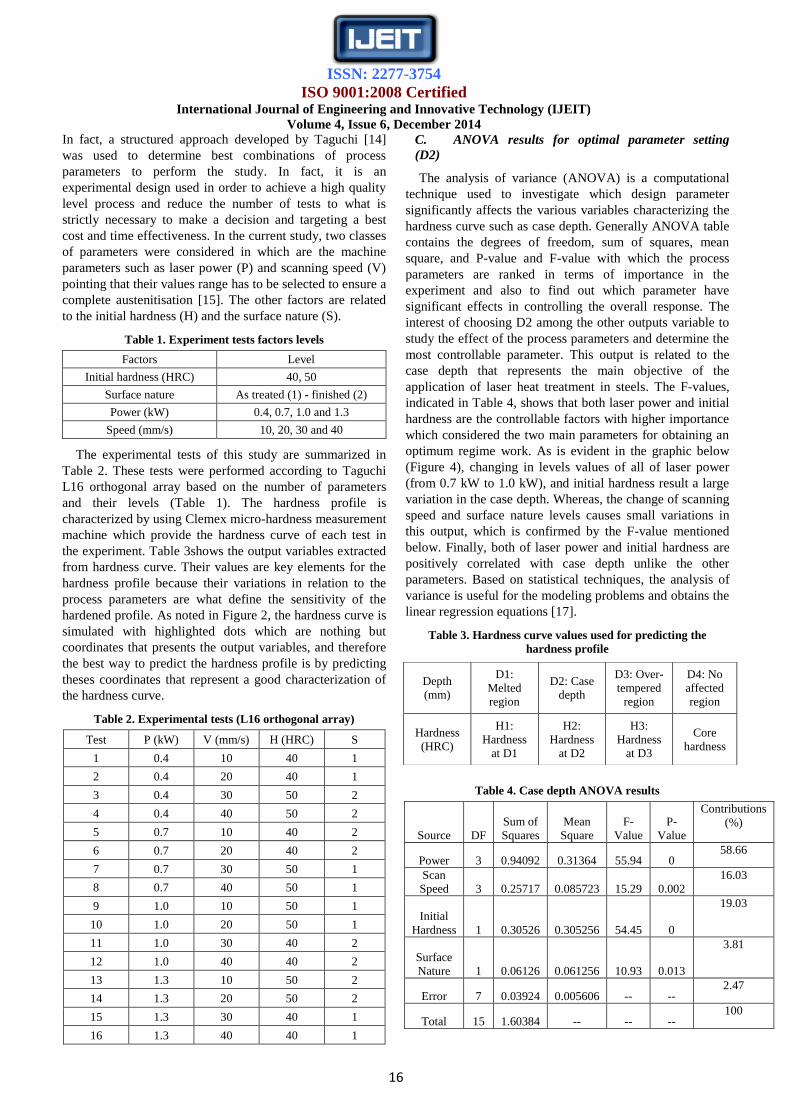
C. ANOVA results for optimal parameter setting
(D2)
The analysis of variance (ANOVA) is a computational
technique used to investigate which design parameter
significantly affects the various variables characterizing the
hardness curve such as case depth. Generally ANOVA table
contains the degrees of freedom, sum of squares, mean
square, and P-value and F-value with which the process
parameters are ranked in terms of importance in the
experiment and also to find out which parameter have
significant effects in controlling the overall response. The
interest of choosing D2 among the other outputs variable to
study the effect of the process parameters and determine the
most controllable parameter. This output is related to the
case depth that represents the main objective of the
application of laser heat treatment in steels. The F-values,
indicated in Table 4, shows that both laser power and initial
hardness are the controllable factors with higher importance
which considered the two main parameters for obtaining an
optimum regime work. As is evident in the graphic below
(Figure 4), changing in levels values of all of laser power
(from 0.7 kW to 1.0 kW), and initial hardness result a large
variation in the case depth. Whereas, the change of scanning
speed and surface nature levels causes small variations in
this output, which is confirmed by the F-value mentioned
below. Finally, both of laser power and initial hardness are
positively correlated with case depth unlike the other
parameters. Based on statistical techniques, the analysis of
variance is useful for the modeling problems and obtains the
linear regression equations [17].
Table 3. Hardness curve values used for predicting the
hardness profile
Table 4. Case depth ANOVA results
Source DF
Sum of
Squares
Mean
Square
F-
Value
P-
Value
Contributions
(%)
Power 3 0.94092 0.31364 55.94 0 58.66
Scan
Speed 3 0.25717 0.085723 15.29 0.002
16.03
Initial
Hardness 1 0.30526 0.305256 54.45 0
19.03
Surface
Nature 1 0.06126 0.061256 10.93 0.013
3.81
Error 7 0.03924 0.005606 -- -- 2.47
Total 15 1.60384 -- -- -- 100
Depth
(mm)
D1:
Melted
region
D2: Case
depth
D3: Over-
tempered
region
D4: No
affected
region
Hardness
(HRC)
H1:
Hardness
at D1
H2:
Hardness
at D2
H3:
Hardness
at D3
Core
hardness

ISSN: 2277-3754
ISO 9001:2008 Certified International Journal of Engineering and Innovative Technology (IJEIT)
Volume 4, Issue 6, December 2014
17
Fig 4. Effect of parameters on the case depth (D2)
III. HARDNESS PROFILE PREDICTION
As previously mentioned, this study aims to predict the
hardness profile of the AISI 4340 heat-treated by Nd: YAG
laser which four parameters were varied. The sequences of
prediction are made by dividing the hardness curve
according to of the four characterizing zones (Figure 2). As
result, these zones can be determined by four points with
their coordinates in terms of depth (mm) and hardness
(HRC) as given in Table 3. The fact that the hardness profile
can be drawn by using these coordinates, good prediction of
the hardness profile can be achieved by predicting those
coordinates. To achieve this goal, two approaches have been
used for prediction; the first was based on artificial neural
networks (ANN), which is a useful prediction tool that can
be implemented successfully in the research and
development of laser surface hardening [16]. The second
approach was based on analytical nonlinear regression.
A. Artificial Neural Network
Neural network is the ideal way of trying to simulate the
brain electronically, as oppose to the generic definition.
Artificial Neural Network (ANN) is term which narrows the
broad definition to the artificial intelligence (AI) research
field. ANN is widely used to challenge an overcome issues
provided by traditional analytical approaches. Several types
of ANN used for modeling such as; feed forward neural
network (FNN), radial basis function network(RBF),
Kohonen self-organizing network (KSON), learning vector
quantization (LVQ) and multilayer perceptron (MLP).
Because of its simplicity and great forecast ability for
modeling, multilayer perceptron (MLP) was used in this
study to learn the mapping characteristics and then to predict
the hardness profile from the experimental conditions
(power (P), scanning speed (S), initial hardness (H) and
surface nature (S)).As defined in numerical computing
software (Matlab), the architecture of the back propagation
neural network consists of three layers depending to the
number of the hidden layers; an input layer where its
neurons number is identical to input parameters number, an
output layer where also its neurons number is identical to
output variables number. Generally, one hidden layer is
sufficient to converge towards the desired model [18]. The
hidden layer consists in 12 neurons that met the requirement
for best prediction of hardness profile. The ANN modeling
architecture is presented in Figure 5.
Fig 5. ANN model architecture
B. Regression model
Among the most known techniques that can model and
analyze problems where some response variables are
influenced by several factors is the response surface
methodology [19]. It can be defined as collection of
mathematical and statistical techniques useful to generate
empirical models that present the relationship between the
input parameters and output responses of the problem. As a
second part of prediction, the present study is based on
response surface methodology to develop mathematical
models with best fits which can represent the relationship
between the interest responses and the process parameters.
A statistical tool was used to develop the approximating
model based on the same observed data that were used to
train Artificial Neural Networks where the purpose is to
compare the suitability of each model for predicting the
outcome variables. Usually, the mathematical formulation of
the approximation model is presented by the following
second order polynomial (equation 1):
(1)
Where: y can be applied to the different output D1, D2,
D3, D4, H1, H2 and H3. The variables
represent Power (W), Scanning speed (mm/s),
Initial hardness (HRC) and nature of surface respectively.
When presents the regression equation constant,
coefficients are linear terms, coefficients are
interaction termsand the coefficients are the quadratic
terms and is the number the process parameters. In order
to obtain mathematical models with best fits, it is critical to
select the number of regressors which they represent the
indeterminate of the model polynomial. The best way to
achieve the appropriate number of regressors for each
outcome regression model was done by an effective
technique. The technique is consists to select a minimum
number possible of regressors and verification of the
matched multiple coefficient of determination (R2).The
process is defined by a continuous increment in the number
of regressors until reaching of the best multiple coefficient
of determination (R2) based on confidence level less than
5%. Table 5 shows the adequate regression coefficients
values and corresponding regressors in the regression
ISSN: 2277-3754
ISO 9001:2008 Certified International Journal of Engineering and Innovative Technology (IJEIT)
Volume 4, Issue 6, December 2014
18
models developed during this study. It is obviously that the
best-fit models are represented by the quadratic form and the
models terms are statistically significant at p-value of less
than 5%. Table 6 presents the result of the analysis of
variance (ANOVA) that used to test the adequacy of the
regression model. The accuracy of the regression model
varies from an output to another according to F-value. Based
on the F-value, the regression model has an excellent ability
to predict D1 and D2, while its prediction accuracy
decreases for the other outputs.
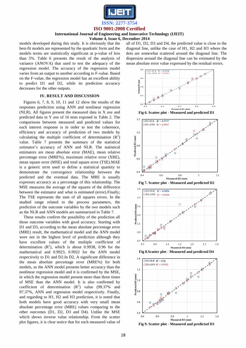
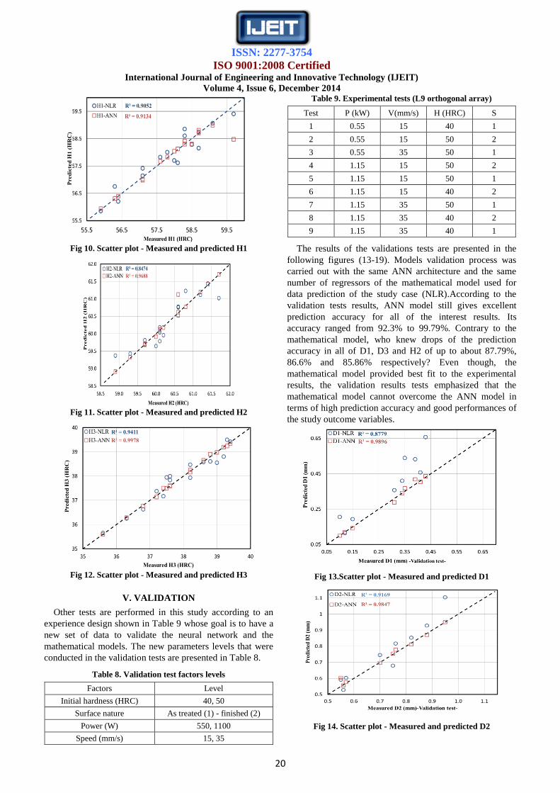
IV. RESULT AND DISCUSSION
Figures 6, 7, 8, 9, 10, 11 and 12 show the results of the
responses prediction using ANN and nonlinear regression
(NLR). All figures present the measured data in X axe and
predicted data in Y axe of 16 tests exposed in Table 2. The
comparisons between measured and predicted values for
each interest response is in order to test the coherence,
efficiency and accuracy of prediction of two models by
calculating the multiple coefficient of determination (R2)
value. Table 7 presents the summary of the statistical
estimator’s accuracy of ANN and NLR. The statistical
estimators are mean absolute error (MAE), mean relative
percentage error (MRE%), maximum relative error (XRE),
mean square error (MSE) and total square error (TSE).MAE
is a generic term used to define a statistical quantity to
demonstrate the convergence relationship between the
predicted and the eventual data. The MRE is usually
expresses accuracy as a percentage of this relationship. The
MSE measures the average of the squares of the difference
between the estimator and what is estimated (error).Finally;
The TSE represents the sum of all squares errors. In the
studied range related to the process parameters, the
prediction of the outcome variables by the two models such
as the NLR and ANN models are summarized in Table 7.
These results confirm the possibility of the prediction all
those outcome variables with good accuracy. Starting with
D1 and D3, according to the mean absolute percentage error
(MRE) result, the mathematical model and the ANN model
were not in the highest level of prediction although they
have excellent values of the multiple coefficient of
determination (R2), which is about 0.9938, 0.96 for the
mathematical and 0.9923, 0.9922 for the ANN model
respectively to D1 and D2.In D2, A significant difference in
the mean absolute percentage error (MRE%) for both
models, so the ANN model presents better accuracy than the
nonlinear regression model and it is confirmed by the MSE,
in which the regression model present more than three times
of MSE than the ANN model. It is also confirmed by
coefficient of determination (R2) value (99.37% and
97.37%, ANN and regression model respectively. Finally,
and regarding to H1, H2 and H3 prediction, it is noted that
both models have good accuracy with very small mean
absolute percentage error (MRE) values comparing to the
other outcomes (D1, D2, D3 and D4). Unlike the MSE
which shows inverse value relationship. From the scatter
plot figures, it is clear notice that for each measured value of
all of D1, D2, D3 and D4, the predicted value is close to the
diagonal line, unlike the case of H1, H2 and H3 where the
dots are somewhat scattered around the diagonal line. The
dispersion around the diagonal line can be estimated by the
mean absolute error value expressed by the residual errors.
Fig 6. Scatter plot - Measured and predicted D1
Fig 7. Scatter plot - Measured and predicted D2
Fig 8.Scatter plot - Measured and predicted D4
Fig 9. Scatter plot - Measured and predicted D3

ISSN: 2277-3754
ISO 9001:2008 Certified International Journal of Engineering and Innovative Technology (IJEIT)
Volume 4, Issue 6, December 2014
19
Table 5. Regression coefficients values and corresponding regressors in the regression models
Outcome Variables D1 D2 D3 D4 H1 H2 H3
-0.44244 -0.17386 0.04256 -0.54781 52.57226 68.8544 33.54686
0.000942 0.001851 0.001009 0.002168 0.024773 -0.02134 0.006167
0.012004 -0.01095 0.012663 0.026769 -0.67722 -0.08168 -0.02581
-4.2E-06 -5.2E-06 -8.3E-06 -1.6E-05 0.000147 4.33E-05 -1.7E-06
-1.8E-05 -4.4E-05 -2.6E-05 -2.9E-05 -0.00067 0.000539 0.000319
6.94E-05 8.06E-05 -5.6E-06 -0.00011 0.001278 -0.00194 -0.00397
-0.00059 -0.00047 -0.00092 -0.00123 0.01242 0.00574 0.00219
0.00545 0.01105 0.01144 0.01087 0.0566 -0.0198 -0.0063
-0.00559 -0.0102 -0.00953 -0.00782 -0.03858 0.035617 0.087031
2.59E-07 4.01E-07 5.01E-07 1.69E-07 1.35E-06 -1.7E-08 -8.6E-06
3.12E-05 0.000156 0.00015 0.000219 -0.00213 -0.00212 0.000188
0.000461 0.000778 0.000728 0.000947 0.004436 -0.00679 -0.0041
No. of regressors 11 11 11 11 11 11 11
Table 6. ANOVA of the mathematical model
Variables Sum of the squares Degrees of freedom
𝐹-ratio R2
Regression Residual Regression Residual
D1 0.809 0.005 14 4 57.735 0.9938
D2 0.816 0.022 14 4 13.448 0.9737
D3 0.899 0.0374 14 4 8.731 0.96
D4 1.580 0.023 14 4 24.866 0.9856
H1 15.215 1.625 14 4 3.405 0.9052
H2 7.116 1.281 14 4 2.019 0.8474
H3 17.621 1.102 14 4 5.811 0.9411
Table 7. Summary of statistical estimators performances - ANN and NLR
Variables
MAE MRE% XRE MSE TSE
R-M ANN-M R-M ANN-M R-M ANN-M R-M ANN-M R-M ANN-M
D1 0.0131 0.0132 5.1309 5.9179 0.0752 0.0796 0.000315 0.000397 0.0050544 0.006363
D2 0.0295 0.0107 4.7073 1.5731 0.1415 0.0889 0.00138 0.0003838 0.02208 0.006132
D3 0.0386 0.0139 5.3244 5.3244 0.1737 0.1021 0.002342 0.000541 0.03747 0.00867
D4 0.0303 0.0245 3.0091 2.0909 0.1376 0.2694 0.001444 0.003982 0.02311 0.06371
H1 0.2656 0.1360 0.4553 0.2196 1.1 1.3379 0.099818 0.101223 1.5971 1.61957
H2 0.219 0.0568 0.3626 0.0940 1.149 0.6103 0.0801 0.018161 1.2816 0.29058
H3 0.2219 0.0404 0.5829 0.1061 0.8935 0.1680 0.0689 0.00257 1.1026 0.041263
ISSN: 2277-3754
ISO 9001:2008 Certified International Journal of Engineering and Innovative Technology (IJEIT)
Volume 4, Issue 6, December 2014
20
Fig 10. Scatter plot - Measured and predicted H1
Fig 11. Scatter plot - Measured and predicted H2
Fig 12. Scatter plot - Measured and predicted H3
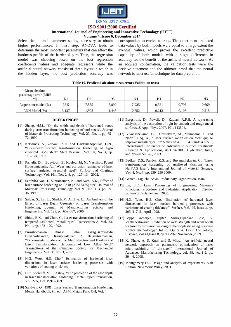
V. VALIDATION
Other tests are performed in this study according to an
experience design shown in Table 9 whose goal is to have a
new set of data to validate the neural network and the
mathematical models. The new parameters levels that were
conducted in the validation tests are presented in Table 8.
Table 8. Validation test factors levels
Factors Level
Initial hardness (HRC) 40, 50
Surface nature As treated (1) - finished (2)
Power (W) 550, 1100
Speed (mm/s) 15, 35
Table 9. Experimental tests (L9 orthogonal array)
Test P (kW) V(mm/s) H (HRC) S
1 0.55 15 40 1
2 0.55 15 50 2
3 0.55 35 50 1
4 1.15 15 50 2
5 1.15 15 50 1
6 1.15 15 40 2
7 1.15 35 50 1
8 1.15 35 40 2
9 1.15 35 40 1
The results of the validations tests are presented in the
following figures (13-19). Models validation process was
carried out with the same ANN architecture and the same
number of regressors of the mathematical model used for
data prediction of the study case (NLR).According to the
validation tests results, ANN model still gives excellent
prediction accuracy for all of the interest results. Its
accuracy ranged from 92.3% to 99.79%. Contrary to the
mathematical model, who knew drops of the prediction
accuracy in all of D1, D3 and H2 of up to about 87.79%,
86.6% and 85.86% respectively? Even though, the
mathematical model provided best fit to the experimental
results, the validation results tests emphasized that the
mathematical model cannot overcome the ANN model in
terms of high prediction accuracy and good performances of
the study outcome variables.
Fig 13.Scatter plot - Measured and predicted D1
Fig 14. Scatter plot - Measured and predicted D2

ISSN: 2277-3754
ISO 9001:2008 Certified International Journal of Engineering and Innovative Technology (IJEIT)
Volume 4, Issue 6, December 2014
21
Fig 15. Scatter plot - Measured and predicted D3
Fig 16. Scatter plot - Measured and predicted D4
Fig 17. Scatter plot - Measured and predicted H1
Fig 18. Scatter plot - Measured and predicted H2
Fig 19.Scatter plot - Measured and predicted H3
Figure 20 shows comparison between modeling and
validation. It is clear to notice that the figure contains three
curves which the black one represent the hardness profile
resulting from the validation (Test 7); while the other curves
are the predicted hardness profiles obtained by the
mathematical model (Blue dashed line) and the ANN model
(Red dashed line).It is clear to note through the form the
Figure 6 that the hardness curve provided by the ANN
model is almost identical to the measured hardness profile,
while there is no similarity between the measured hardness
profile and hardness curve provided by the mathematical
model (NLR). This means that the ANN model has a better
fit of the experimental results and provides a better
prediction of the hardness profile than the traditional
nonlinear regression model. Table 10 confirms that the
performances demonstrated by ANN model are superior
comparing to those produced by nonlinear regression. In
fact, the precision of ANN model of overall hardness curves
characterized by the variables Di and Hi is less than 4%.
Fig 20. Predicted and measured hardness curves (Validation -
Test 7)
VI. CONCLUSION
The paper presented a comparison study between two
prediction models used to evaluate the hardness profile of
plates made of 4340 and heat-treated by laser. Experimental
data used for the prediction are obtained by performing tests
through orthogonal arrays using Taguchi design in order to
ISSN: 2277-3754
ISO 9001:2008 Certified International Journal of Engineering and Innovative Technology (IJEIT)
Volume 4, Issue 6, December 2014
22
Select the optimal parameter setting necessary to obtain
higher performances. In first step, ANOVA leads to
determine the most important parameters that can affect the
hardness profile of the hardened part. Then, the regression
model was choosing based on the best regression
coefficients values and adequate regressors while the
artificial neural network consist of three layers in which in
the hidden layer, the best prediction accuracy was
correspondent to twelve neurons. The experiment predicted
data values by both models were equal to a large extent the
eventual values, which proves the excellent predictive
capability of both models with a slight difference in
accuracy for the benefit of the artificial neural network. As
an accurate confirmation, the validation tests were the
decisive statement and the ultimate proof that the neural
network is most useful technique for data prediction.
Table 10. Predicted absolute mean error (Validation tests)
REFERENCES
[1] Shang, H.M., “On the width and depth of hardened zones
during laser transformation hardening of tool steels”, Journal
of Materials Processing Technology, Vol. 23, No. 1, pp. 65–
72, 1990.
[2] Katsamas, A., Zervaki, A.D. and Haidemenopoulos, G.N.,
“Laser-beam surface transformation hardening of hypo
eutectoid Ck-60 steel”, Steel Research, Vol. 68, No. 3, pp.
119–124, 1997.
[3] Pantelis, D.I., Bouyiouri, E., Kouloumbi, N., Vassiliou, P. and
Koutsomichalis, A., “Wear and corrosion resistance of laser
surface hardened structural steel”, Surface and Coatings
Technology, Vol. 161, Nos. 2–3, pp. 125–134, 2002.
[4] SenthilSelvan, J., Subramanian, K., and Nath, A.K., Effect of
laser surface hardening on En18 (AISI 5135) steel, Journal of
Materials Processing Technology, Vol. 91, No. 1–3, pp. 29–
36, 1999.
[5] Safdar, S., Lin, L., Sheikh, M. A., Zhu. L., An Analysis of the
Effect of Laser Beam Geometry on Laser Transformation
Hardening, Journal of Manufacturing Science and
Engineering, Vol. 128, pp. 659-667, 2006 .
[6] Shiue, R.K., and Chen, C., Laser transformation hardening of
tempered 4340 steel, Metallurgical Transactions A, Vol. 23,
No. 1, pp. 163–170, 1992.
[7] Purushothaman Dinesh Babu, Gengusamynaidu
Buvanashekaran, Karupuudaiyar R. Balasubramanian,
“Experimental Studies on the Microstructure and Hardness of
Laser Transformation Hardening of Low Alloy Steel”
Transactions of the Canadian Society for Mechanical
Engineering, Vol. 36, No. 3, 2012.
[8] H.G. Woo, H.S. Cho,” Estimation of hardened layer
dimensions in laser surface hardening processes with
variations of coating thickness.
[9] H.R. Shercliff, M. F, Ashby, “The prediction of the case depth
in laser transformation hardening”. Metallurgical transaction,
Vol. 22A, Oct. 1991-2459.
[10] Sandven, O., 1981, Laser Surface Transformation Hardening,
Metals Handbook, 9th ed., ASM, Metals Park, OH, Vol. 4.
[11] Bergstrom, D.; Powell, D.; Kaplan, A.F.H. A ray-tracing
analysis of the absorption of light by smooth and rough metal
surfaces. J. Appl. Phys. 2007, 101, 113504.
[12] Buvanashekaran, G., Duraiselvam, M., Manoharan, S. and
Noorul Haq, A., “Laser surface modification technique to
improve metallurgical properties of AISI 304 stainless steel”,
International Conference on Advances in Surface Treatment:
Research & Applications, ASTRA-2003, Hyderabad, India,
and November 3–6, 2003.
[13] Badkar, D.S., Pandey, K.S. and Buvanashekaran, G., “Laser
transformation hardening of unalloyed titanium using
Nd:YAG laser”, International Journal of Material Science,
Vol. 4, No. 3, pp. 239–250 2009.
[14] Genichi Taguchi, Asian Productivity Organization, 1986.
[15] Ion, J.C., Laser Processing of Engineering Materials
Principles, Procedure and Industrial Application, Elsevier
Butterworth-Heinemann, 2005.
[16] H.G. Woo, H.S. Cho, “Estimation of hardened layer
dimensions in laser surface hardening processes with
variations of coating thickness”. Surface, Vol.102, Issue 3, pp.
205–217, 21 April 1998.
[17] Bappa Acherjee, Dipten Misra,Dipankar Bose, K.
Venkadeshwaran `Prediction of weld strength and seam width
for laser transmission welding of thermoplastic using response
surface methodology’ Jnl. of Optics & Laser Technology,
Elsevier, Vol 41,Issue 8, pp.956-967,November ,2009.
[18] K. Dhara, A. S. Kuar, and S. Mitra, “An artificial neural
network approach on parametric optimization of laser
micromachining of die-steel,” International Journal of
Advanced Manufacturing Technology, vol. 39, no. 1-2, pp.
39–46, 2008.
[19] Montgomery DC. Design and analysis of experiments. 5 th
Edition. New York: Wiley; 2001.
Mean absolute
percentage error (MRE
%) D1 D2 D3 D4 H1 H2 H3
Regression model (%) 36.5 7.555 5.899 7.935 0.581 0.796 0.669
ANN Model (%) 3.137 1.908 1.445 0.652 0.213 0.108 0.215