prediction intervals for future demand of existing products with an observed demand of zero

ARTICLE IN PRESS

Contents lists available at ScienceDirect

Int. J. Production Economics

Int. J. Production Economics 119 (2009) 75–89

0925-52

doi:10.1

� Cor

E-m

journal homepage: www.elsevier.com/locate/ijpe

Prediction intervals for future demand of existing products with anobserved demand of zero

Matthew Lindsey a,�, Robert Pavur b

a College of Business & Technology, University of Texas at Tyler, 3900 University Boulevard, Tyler, TX 75799, USAb ITDS Department, University of North Texas, P.O. Box 305249, Denton, TX 76203, USA

a r t i c l e i n f o

Article history:

Received 12 January 2008

Accepted 23 January 2009Available online 1 February 2009

Keywords:

Intermittent demand

Prediction intervals

Simulation

Poisson process

73/$ - see front matter & 2009 Elsevier B.V. A

016/j.ijpe.2009.01.006

responding author. Tel.: +1903 565 5807; fax:

ail address: [email protected] (M. Lin

a b s t r a c t

A proposed technique for forming reliable prediction intervals for the future demand

rate of existing products with observed demand of zero is illustrated using methodology

adapted from software reliability. By using the demand information from a group

of products which includes slow-moving products, prediction intervals for the future

demand rate of the products with an observed demand of zero are constructed. A

simulation study examined the reliability of these prediction intervals across

experimental conditions that included product group size, mean time between demand,

and Type I error levels. The proposed prediction intervals had empirical Type I errors

closer to their nominal values when there were a sufficient number of products with no

sales and also with some sales.

& 2009 Elsevier B.V. All rights reserved.

1. Introduction

The phenomenon of positive demand followed byextended periods of no demand occurs in numerousbusiness situations (Chatfield and Hayya, 2007). When aperiod of zero demand is observed for an existing product,a zero forecast for future demand may be a reasonableestimate for a product at the end of its life cycle.Alternatively, an estimate of zero for a product’s futuredemand may be too conservative if the product is merelyslow moving. Perhaps the period over which demand isobserved is too short to establish an accurate forecast forfuture demand. Dolgui and Pashkevich (2008) state that acommon difficulty in forecasting slow-moving inventoryis the lack of information about demand. Due to fluctua-tions in customer buying patterns resulting in randomperiods of no demand, a product’s demand may appear tobe zero, but its future demand may still be large enough towarrant carrying the product in the long run.

ll rights reserved.

+1903 566 7372.

dsey).

The estimated future demand rate for products is onecriterion used to determine the feasibility of keeping thatproduct in inventory. The research in this paper addressesthe issue of estimating the future demand rate of a groupof products that display no demand. These products arenot new products, but products whose demand has beenobserved over a specified period. If a product’s demand issmooth and continuous, traditional forecasting methodsoften provide reasonable estimates of its future demandrate.

Inventory management in an environment with pro-ducts experiencing intermittent demand can be tenuous,with little information to accurately forecast demand forany one product. Miragliotta and Staudacher (2004)examine how unstructured information such as expecta-tions about order placement probability can be embeddedinto the management of intermittent orders. To obtainimproved forecasts, knowledge of aggregate data has beenused in forecasting. Dalhart (1974) proposed productaggregation and illustrated substantial improvements inestimating seasonal indices with aggregate data. Studiessuch as Dekker et al. (2004) and Caniato et al. (2005)illustrate the potential improvement of using forecasting

www.sciencedirect.com/science/journal/proeco

www.elsevier.com/locate/ijpe

dx.doi.org/10.1016/j.ijpe.2009.01.006

mailto:[email protected]

ARTICLE IN PRESS

M. Lindsey, R. Pavur / Int. J. Production Economics 119 (2009) 75–8976

procedures with aggregated demand information overclassical methods of forecasting.

In contrast to aggregating data or forecasts for acombined set of data, an approach used in our paperemploys information about the demand of ‘‘peripheral’’products to predict the demand rate for a pool of productsthat have exhibited no observed demand over a specifiedtime period. This pool of products is a subgroup of a largergroup of products, some or all of which may be slowmoving. Using zero as the estimate of future demandmay be too little for products exhibiting zero demand.For example, the demand estimate may be conservativebecause the period in which demand is observed is tooshort to obtain accurate demand information. In ourresearch, observed products include this pool of productswith zero demand and the ‘‘peripheral’’ products thatshow positive demand. Unlike aggregate forecasting inwhich a forecast is made for the entire group, a proposeddemand estimate is made only for that pool of productsthat demonstrated zero demand.

Instead of assessing the accuracy of the estimate ofthe demand rate, our paper assesses the reliabilityof proposed prediction intervals for the demand rate. Thisassessment is made via a simulation study. Underlyingassumptions for the demand of the products are similar tothat used in previous studies that model slow-movinginventory. These assumptions are that products haveindependent demand and that the demand of a productfollows a Poisson process (Gelders and Van Looy, 1978;Bagchi et al., 1983; Schultz, 1987; and Johnston andBoylan, 1996). Dolgui and Pashkevich (2008) remarkthat the Poisson probability distribution dominates theresearch devoted to modeling product demand. Thesesame assumptions are used in our study in constructingprediction intervals for the demand rate of products withno observed demand. The slow-moving inventory thatwould be appropriate for the proposed models shouldhave an average demand per period that is low eitherbecause demand is infrequent or due to low averagedemand as defined by Boylan et al. (2008). Items withlumpy demand, such as demand derived from a materialsrequirement planning (MRP) system would not be appro-priate for the proposed model. Definitions of types ofslow-moving inventory are provided in Section 2.2.

Why examine the reliability of prediction intervals onthe demand rate of a group of products rather than focussolely on the accuracy of the demand rate itself? Supplychain managers require a reliable estimate of both theexpected demand rate and the estimate’s variance todetermine safety stock levels. Shenstone and Hyndman(2005) explain that underlying stochastic models can beused to construct prediction intervals for the purposesof obtaining safety stock levels. The upper and lowerlimits of a prediction interval for demand provide a rangefor the appropriate level of safety stock. Also, a singleestimate of demand rate may be misleading if the varianceis large. If the upper limit of the estimated demand ratefor a group of products is below an economically basedthreshold of demand, then a manager may have sufficientjustification to discontinue keeping the products ininventory. Shenstone and Hyndman (2005) compute

prediction intervals for the monthly demand for a servicepart for Saturn motor vehicles. Gardner (2006) discusseshow prediction intervals can be formed for variousforecasting methods.

Improved methodologies for constructing reliableprediction intervals for the future demand of slow-movingretail products are desirable for several reasons. First,sometimes incidental products, such as cufflinks at amen’s clothing store, need to be carried because theyare expected to be available. A company may even havea critical product that must be maintained althoughthe sales are sporadic. In these cases, managementmust determine an appropriate level of inventory tocarry. Second, the underlying demand distribution may bedifficult to estimate if observable sales are not available.More efficient techniques for predicting future demandsfor slow-moving inventories can lower holding costs,minimize obsolescence, reduce required working capital,increase cash flows, as well as improve the ability to fulfillcustomer orders.

In this research, prediction intervals for the futuredemand rate of slow-moving inventory will be proposedand assessed. The proposed prediction intervals for futuredemand rates of products with no sales and theirperformance over a variety of conditions has not beenpreviously explored. Prediction intervals account for boththe point estimate of future demand rate and its stand-ard deviation. The literature does not present or assessthis methodology for addressing the difficult problem ofestimating future demand rates for products with limitedor no demand over a specified time period. This studyassesses the robustness of the reliability of two-sidedprediction intervals (TSPIs) for the future demand rate ofexisting products with no observed demand.

2. Research background

2.1. Inventory control

To cope with the challenges of efficiently controllinginventory, companies have invested heavily in computersoftware packages such as MRP, manufacturing resourceplanning (MRPII) or enterprise resource planning (ERP)systems. The MRP software generally contains a materialprocurement module that handles the inventory manage-ment function by calculating the safety stock and reorderpoint based on a product’s demand history to ensure thatthe right part is at the right place when needed (Ornekand Cengiz, 2006). These integrated modules enhance thesoftware’s ability to forecast demand for fast-movingproducts, but often they perform poorly for products withintermittent demand (Razi and Tarn, 2003).

Relatively few products often represent the bulk of therevenue and the majority of the demand in the manu-facturing sector of the economy. These products aretypically the faster selling products. If a product has notsold over a specified duration of time, its demand wouldbe projected to be zero based on many of the popularforecasting models. Yet, this product may still sell enoughin the future to be worth carrying particularly if the

ARTICLE IN PRESS

M. Lindsey, R. Pavur / Int. J. Production Economics 119 (2009) 75–89 77

inventory cost is well managed. Our research will proposea methodology for predicting demand rates for intermit-tent or slow-moving merchandize that is adapted fromstatistical procedures developed for software reliability.

2.2. Definition and examples of slow-moving inventory

The methodology in this research is to observe a groupof products, which may even be a mixture of fast-movingand slow-moving goods, over a fixed time period, and thenconstruct a prediction interval for the future demandof the pool of products with observed demand of zero. Thedemand for each individual product both over the fixedtime period in which demand is observed and over futuretime periods is assumed to approximately follow aPoisson process. Since the demand for all products followa Poisson process, the products displaying no demand alsofollow a Poisson process. The classification of the demandpattern for these products may fall into one of the ‘‘slow’’categories defined by Boylan et al. (2008). A product withno history of demand could be considered slow-moving

and such a product is considered to have an averagedemand per period that is low. A product is slow movingbecause of ‘‘infrequent demand occurrences, low averagedemand sizes or both.’’ However, Boylan et al. (2008) statethat their framework is conceptual, rather than opera-tional, since ‘‘high’’ and ‘‘low’’ are not quantified. Manage-ment determines what is ‘‘low.’’ Boylan et al. (2008)classifies a product as intermittent if it is ‘‘an item withinfrequent demand occurrences.’’ Altay et al. (2008)suggest that products having zero demand more than30% of the time be classified as intermittent. Boylan et al.(2008) classifies a product as erratic if it is ‘‘an item whosedemand size is highly variable’’ and as lumpy if it is ‘‘anintermittent item for which demand, when it occurs, ishighly variable.’’ Erratic demand is characterized by a highcoefficient of variation. For the case of erratic or lumpydemand, the assumption of a product’s demand followinga Poisson process is not reasonable. Boylan et al. (2008)classifies a product as clumped if it is ‘‘an intermittent itemfor which demand, when it occurs, is constant (or almostconstant)’’.

Miragliotta and Staudacher (2004) present a historicalperspective on lumpiness in the academic literature so asto depict the ‘‘awareness path’’ to it. In our research, theterm slow moving is used to refer to demand character-ized by periods of zero demand. The proposed methodol-ogy in this paper is suitable for forecasting any of thespecial cases in the ‘‘slow’’ category provided that thedemand over the specified period is assumed to approxi-mately follow a Poisson process. Masters (1993) notedthat large retailers might have thousands of stock keepingunits (SKUs) that sell at a rate of only two or three permonth per store. Porras and Dekker (2008) classified2,226 items out of 8,494 spare parts used in their analysisof various re-order point methods to be suitable for thePoisson model. Considerable research has centered on theuse of the Poisson process in inventory management.Dolgui and Pashkevich (2008) state that slow-movingSKUs often has a demand pattern that can be represented

as a binary vector. In addition, they remark that theclassical way to model this type of slowing inventory isbased on the Poisson distribution.

Masters (1993) claims that a reasonable assump-tion for the demand of many retail products is thatthe demand follows a Poisson process. Masters (1993)explains that in the case where a relatively large numberof independent customers can be assumed to have anequal but small probability of purchasing a product, thePoisson distribution is appropriate. These retail productsmay be slow moving, but cannot be lumpy or discontin-uous with highly variable sales, for this assumption tohold. Censored products from groups of products thatfollow a Poisson process also follow a Poisson processaccording to Masters (1993). Thus, subgroups of groups ofproducts that follow a Poisson process also have thisunderlying assumption.

2.3. Forecasting methods for slow-moving goods

Many of the existing approaches to estimating de-mands for slow-moving products find their roots inresearch related to predicting usage rates for militaryspare parts, especially those onboard ships (Haber andSitgreaves, 1970). Haber and Sitgreaves (1970) surveyseveral forecasting methods for goods with sporadicdemand patterns, including a method that relies on expertopinion to pool usage figures for products with similardesigns. These items would for the most part be classifiedas having lumpy demand and would not follow theassumption of demand following a Poisson distribution.A limitation is that the number of categories to whichparts are classified needs to be determined to providesufficient data to obtain reliable estimates of demand.Their approach differs from the approach in this paper.Our approach first selects a group of products, some or allof which may be slow moving. Unlike forecasting thedemand for the entire group of products, our approachproposes a prediction interval for the demand rate of onlythe pool of products that have a demand of zero over aspecified time period in which demand is observed.

Unfortunately, many approaches to increasing produc-tivity, such as MRP II, depend on accurate forecasts(Willemain et al., 1994). Traditional methods for solvingthis problem are proposed by Haber and Sitgreaves (1970),Burton and Jaquette (1973), Croston (1972), and Williams(1984). Syntetos and Boylan (2001) proposed a modifiedmethod based on Croston’s procedure (1972) that cor-rected a suspected bias. These various methods generallysuggest different ways of classifying products and esti-mate demand for items in each category by using anappropriate technique. Altay et al. (2008) propose amodification of Holt’s method to forecast intermittentdemand when a trend is present based on the firmscompetitive priorities. Furthermore, Altay et al. (2008)provide an excellent and succinct literature review offorecasting demand for slow-moving items.

Silver (1965), Brown and Rogers (1973), and Smithand Vemuganti (1969) offer Bayesian approaches to fore-casting the demand for slow-moving goods based on

ARTICLE IN PRESS


historical data, which are often not available. Muckstadtand Thomas (1980), Silver (1970), and Thompstone andSilver (1975) have suggested additional models for specialcases involving slow-moving items. Leven and Segerstedt(2004) propose an ERP system implementation based onthe Croston’s (1972) method that is capable of forecastingslow-moving and fast-moving products; however theirapproach was criticized for being biased (Boylan andSyntetos, 2007). In addition to emphasizing the impor-tance of the distribution of demand, Sani and Kingsman(1997) also suggest that the variance of the forecast isan important factor in determining a proper method.Willemain et al. (2004) develop a distribution indepen-dent bootstrap method for estimating intermittent de-mand, which was demonstrated to outperform some ofthe above-mentioned methodologies. Altay et al. (2008)discuss bootstrapping and compare Croston’s method to amodified version of Holt’s method applied to forecastingdemand for spare parts.

2.4. Software reliability

In our research, prediction methodology used in soft-ware reliability is adapted for the study of slow-movinginventory. Many models based on the Poisson distribu-tion have been considered for estimating failure rates insoftware (Abdel-ghaly et al., 1986; Kaufman, 1996). Ascomputer software packages are developed, rigorous testingis required to identify faults or bugs before they are releasedto the customer. The rates of the occurrence of bugs havebeen found to follow a variety of distributions in addition tothe Poisson, including the exponential, gamma, Weibull,and geometric distributions (Abdel-ghaly et al., 1986; Miller,1986). However, Abdel-ghaly et al. (1986) suggest thatno one distribution has been shown to be superior to othersin forecasting the number of bugs a priori, leaving theprogrammer to determine which distribution best fits thehistorical data according to its predictive ability.

Ross (2002) proposes a statistical method for estimat-ing software reliability based on the occurrence of bugsfollowing a Poisson distribution. Since the estimationof the future demand rate for a pool of products with nohistory of demand will use methodology similar to thisprocedure, Ross’ (2002) approach will be presented in theremainder of this section. Note that bugs can be thoughtof as being products and a detected bug can be thought ofas a sale. An estimate of the future occurrences of errors isneeded on the bugs that have no history of error and areundetected. In inventory management, an estimate of thefuture demand rate is needed on the products with nohistory of demand.

The future error rate of bugs in a software applicationthat have not revealed any errors over a specified timeperiod can be estimated by using the information aboutother bugs that have only revealed one or two errors. In asimilar fashion, the future demand rate of products thathave not revealed any observed demand over a specifiedtime period can be estimated by using information aboutother products that have only revealed one or two sales.The assumption that the distribution of the errors in

software reliability and that the distribution of demand ofproducts follows a Poisson distribution are both sup-ported in the literature for each application. Because theassumptions, such as bugs and products acting indepen-dently and entities revealing no past occurrences, arethe same, the statistical techniques are applicable toboth problems. These techniques will be used to predictdemand for slow-moving products as described in thefollowing paragraphs. In particular, the estimator for theerror rate of bugs that have not revealed any errors(labeled M1ðtÞ=t below) is the statistic in which the countof the number of bugs from the total group of bugsthat have observed exactly one error is divided by theobserved time. For slow-moving products, the estimatorfor the demand rate of products with observed demandof zero is the statistic that divides the time for observingthe demand of a group of products into the count of thenumber of products with exactly one sale. This paperextends Ross (2002)’s approach by proposing predictionintervals for demand of products revealing no observeddemand and using a simulation study to assess thereliability of these intervals.

In the context of estimating demand for slow-movinginventory, the notation mentioned for software reliabilitycan be interpreted as shown below. In this study, L(t) willrepresent the demand rate for slow-moving productsthat have not experienced a previous sale over a specifiedperiod of time. By definition, L(t) is the sum of thetheoretical underlying demand rates for unsold products.

n number of productsli demand rate for product i, i ¼ 1,2,y,nt length of time period over which demand is

observedCi(t) equal to 1 if product i has no sales by time t and

0 otherwiseL(t) theoretical mean demand rate of products

experiencing no salesMj(t) number of products that have sold exactly j

items by time t

M1ðtÞ=t estimator of L(t)M1ðtÞ þ 2M2ðtÞ=t2 estimator of mean squared difference

between M1ðtÞ=t and L(t)

Suppose that there are n bugs contained in a softwarepackage. The number of errors caused by bug i is assumedto follow a Poisson distribution with a mean of li,i ¼ 1,2,y,n. Ross (2002) defines Ci(t) ¼ 1 if bug i has notcaused a detected error by time t40 and 0 otherwise,i ¼ 1,2,y,n. These indicator variables allow the remainingerror rate, which is the number of times an error willoccur for the remaining bugs, to be expressed as (1).This equation is an expression for the future error rateof the bugs that remain in the software because they havenot been detected over a specified time frame. That is, (1)expresses the remaining or future error rate. Estimatingthis quantity is important in the decision-making processof releasing the software to the market. Obviously, ahigh error rate would be unacceptable to the customer. Inthe context of slow-moving products, (1) represents thefuture demand rate of products that have not exhibited

ARTICLE IN PRESS


any demand over a specified time frame. That is, thisequation expresses the demand rate of products whoseobserved demand is zero. If the future demand of theseslow-moving products is high enough, a manager maydecide that the products are worth keeping in inventory.

LðtÞ ¼Xn

i¼1

liCiðtÞ (1)

To estimate L(t), Ross (2002) uses Mj(t) to denote thenumber of bugs that are responsible for j detected errorsby time t, j ¼ 1,2,y,n. For instance M1(t) is the numberof bugs that cause exactly one error, M2(t) is the number ofbugs that cause exactly two errors, and so on withPn

i¼1jMjðtÞ being the total number of detected errors. Itis shown in (2) that E½LðtÞ �M1ðtÞ=t� ¼ 0, which estab-lishes that M1ðtÞ=t is an unbiased estimate of the expectedvalue of L(t). The second moment of LðtÞ �M1ðtÞ=t is thesame as the expected value of M1ðtÞ þ 2M2ðtÞ=t2, which isa function of two computationally easy statistics �M1(t)and M2(t). Therefore, the mean squared difference be-tween L(t) and M1ðtÞ=t can be estimated by M1ðtÞþ

2M2ðtÞ=t2. These expressions are summarized in (2).

E½M1ðtÞ� ¼Pni¼1

lite�li t

E½LðtÞ� ¼Pni¼1

liE½CiðtÞ� ¼Pni¼1

lie�li t

E M1ðtÞt

h i¼ E½LðtÞ�

E½M2ðtÞ� ¼12

Pni¼1

ðlitÞ2e�lit

E LðtÞ � M1ðtÞt

h i2� �

¼Pni¼1

l2i e�li tþlie

�li t

t

� �¼

E½M1ðtÞ�þ2M2ðtÞ�t2

(2)

Note that the estimator for the expected future rate andits deviation from the theoretical demand rate shouldhave appeal to practitioners since M1(t) and M2(t) aresimply counting functions. In addition to errors from abug following a Poisson process, Ross (1985a) makes twobasic assumptions: bugs are independent and there is aprobability p of detecting a bug. In the context of slow-moving inventory, these two assumptions are incorpo-rated by assuming that the demand of each product isindependent of the demand of other products and thatthe probability of detecting a sale is equal to one; thatis, demand is detected with 100% certainty. However,Ross (2002) does not discuss the distribution of theseestimators, nor does he propose the use of predictionintervals.

3. Methodology

3.1. Estimating demand rate for a family of products with

zero demand

The same statistic used in estimating the future erroroccurrence rate in newly released software with all knownbugs removed is also the statistic that can be used toestimate the future occurrence rate of product sales after

exhibiting no sales over a specified time period. Accordingto Ross (1985a, b, 2002), the estimated error rate of asoftware package after debugging is equal to the numberof bugs that caused exactly one error, M1(t), divided by thelength of the testing period t in which these errors occur,that is, M1ðtÞ=t. It is possible for the error rate of each bugto be different although knowledge of the number oferrors caused by each detected bug is required. Hence, thedemand rate for each product could be different as well inconstructing prediction intervals for demand rates.

The distribution of the estimate of the future demandrate, M1ðtÞ=t, is examined via simulation. An illustrationof the effect of the product group size on the distributionof M1ðtÞ=t is presented in Fig. 3. Note that a product witha mean time between demand (MTBD) of 300, whichindicates that the expected time between consecutivedemands of a product is 300 time periods, would beconsidered relatively slow-moving over a time interval of100 periods. The distribution of M1ðtÞ=t is affected by boththe MTBD and the product group size.

As illustrated by the histograms in Fig. 3, the normalapproximation for the distribution of M1ðtÞ=t is not asgood for a product group size of 50 as for a size of 200. Ifthe skewness coefficient is sufficiently large in magnitudeunder a particular set of parameters, then the normaldistribution may not be a good approximation of thedistribution of M1ðtÞ=t. Also, there has to be enoughproducts that exhibit exactly one sale for the distributionof M1ðtÞ=t to approximately follow a normal distribution.For example, if all the products were fast moving, say witha MTBD of 10, then there would be very few productsobserved over 100 time periods that displayed either oneor zero demand. Hence, this study did not considerproducts with a MTBD of less than 50 since those productsyield few products with zero demand over a time frameof 100 periods. The simulation study in this paper willdetermine if the normal approximation used in the predi-ction intervals provides reliable estimates. After simulat-ing the distribution of M1ðtÞ=t to understand the shape ofits distribution, it is proposed that a normal distributionmay be a reasonable approximation, but the goodnessof fit for this approximation is dependent on the lengthof the observed period, the demand rates of products,and the number of products in the inventory system. Theproposed prediction intervals with 100(1�a)% confidencewill be of the form presented in (3) for products with nohistory of demand. The future demand rate may not bereliable if the actual distribution of M1ðtÞ=t is too skewed.Under certain parameter values such as a small productgroup size, the value of Za/2 in (3) may be too smallbecause of the magnitude of the skewness coefficient ofthe distribution of this estimator may be too large. That is,the nominal (stated) confidence level of (3) will no longerhold if the normal distribution is not a good approxima-tion of a distribution that is skewed. The reliability of suchintervals will be assessed over a variety of demand ratesand numbers of products.

M1ðtÞ

t� Za=2

ffiffiffiffiffiffiffiffiffiffiffiffiffiffiffiffiffiffiffiffiffiffiffiffiffiffiffiffiffiffiffiffiffiM1ðtÞ þ 2M2ðtÞ

t2

s(3)

ARTICLE IN PRESS


Note that M1ðtÞ=t is an attractive estimator, bothbecause it is an unbiased estimator of the expected valueof L(t) and because it can be easily computed in practice.Importantly, the variance of the difference of M1ðtÞ=t andL(t) or equivalently their expected squared differencedecreases over time as illustrated in (2). Furthermore,from (2), note that if the demand rate, li, is large, then theterm lie

�lit is small for i ¼ 1,2,y,n. Thus, in this case, theexpected value expression of M1(t) implies that therewould be a small number of products with only one sale.Thus, it is expected that M1ðtÞ=t will be small in the casewhen most products have high demand. In addition, notethat if t is large, M1ðtÞ=t will be small, thus implying a lowdemand rate for products that have not experienced a saleby time t. This is intuitive since a product with no demandover a very long time has little expectation of demand forthe future. An unbiased estimator of the squared differ-ence between L(t) and M1ðtÞ=t is M1ðtÞ þ 2M2ðtÞ=t2 asshown in (2). Since the expected value of this estimator isPn

i¼1l2i e�lit þ lie

�lit=2, the expected squared differencebecomes small when t is large and a small expectedsquared difference is desirable.

A natural question to ask is: How large should n

and t be so that the squared difference between L(t) andM1ðtÞ=t is sufficiently small? To address this question, abound on E[(L(t)�M1(t)/t)2] is derived as follows. First,the value of li that maximizes E[(L(t)�M1(t)/t)2] iscomputed. This value can be found by finding themaximum of the function f ðliÞ ¼ ðl

2i þ li=tÞe�lit ; i ¼

1;2;3; . . . ;n: The solution is given by (4) and verified tobe a maximum by the value of the second derivative in (5).

li ¼2� t þ

ffiffiffiffiffiffiffiffiffiffiffiffiffit2 þ 4

p2t

(4)

d2f ðliÞ

dl2i

¼ e�li t �


pt

" #; where li is given by ð4Þ (5)

A bound for the expected squared difference of L(t) andM1ðtÞ=t is stated in (6). Details of this derivation arepresented in Appendix A.

E LðtÞ �M1ðtÞ

t

� �2" #

p1:07n

t2assuming tX2 (6)

The value of t in (6) was assumed to be at least two sothat the constant 1.07 was small and close to a roundnumber like 1.0. Selecting the value of t to be larger wouldprovide a lower bound. This bound provides the practi-tioner with an upper limit for the expected squared errorwith knowledge of only n (number of total productsobserved) and t (time frame for observing demand). Thus,n and t can be selected in practice to provide a bound onthe expected squared error.

3.2. Product group and time frame used to assess proposed

prediction intervals

The term product group will be used to denote a groupor mixture of products, which may be dissimilar infeatures, but could be similar in either demand rates ora mixture of high and low demand rates. The term time

frame will refer to the length of time in which demandfor products is observed before computing the proposedprediction intervals. An implicit assumption of the simu-lation is that the demand for a product is independentof the demand for other products. Prediction intervals willbe referred to as being robust if they maintain their nominalType I error rate over a variety of experimental conditions.

An appropriate time frame needed to be selected toobserve simulated demand. After preliminary experimen-tation, a time frame of 100 time units was selected. Thischoice provided sufficient time to observe the demand ofslow-moving products over a variety of demand rates andstill be able to assess the performance of the proposedprediction intervals. Although a 100 time observationsappears to be a stiff restriction, a large sample size is notuncommon in forecasting. Note that for an ARIMA modelthat Box et al. (1994, p. 17) recommend, ‘‘yat least 50 andpreferably 100 observations or more should be used.’’ Forcertain demand rates, the proposed prediction intervalsare robust for a smaller number of time units, but 100 wasused to illustrate the efficacy of the proposed intervals.

It should be noted that time units can be hours, days,weeks, months, or quarters. For example, the time frameof 100 units can approximate one calendar quarter(90 days) if the time unit is days or 2 years (104 weeks)if the time unit is weeks. If the time unit is monthsor some larger period of time, this model would notbe appropriate and would require an excessive period oftime to gather the information. The prediction intervalsare used to forecast only the demand rate of productshaving zero observed demand, not the demand rate of theentire group of products both with and without demandhistory as in studies that aggregate products. The demandrate will be expressed in terms of MTBDs.

3.3. Interpreting prediction intervals for transaction rate

under compound Poisson assumption

For spare parts inventory, the number of items whosedemand is lumpy may be high, as much as 90%as indicated by a Vereecke and Verstraeten’s (1994)study using spare parts from a large chemical plant. Acompound Poisson process has been suggested as a modelfor lumpy demand (Porras and Dekker, 2008). A com-pound Poisson process allows for the transactionsor demand occurrences to follow a Poisson process, butfor the demand to be other than unit sized. That is, ateach demand transaction, a random variable is used tomodel the size of the demand, which may vary widely.The proposed prediction intervals can be used to forecastthe rate of demand occurrence for the entire group ofproducts having zero observed demand. The statistic Mj(t)needs to be redefined to be the number of products thathave exactly j demand occurrences by time t. Demand sizewould need to be analyzed separately. Porras and Dekker(2008) note that the two-parameter gamma distributionhas been proposed to fit demand size.

Thus, for the case of lumpy demand that followsa compound Poisson process, the results in this studyare useful for predicting the future rate of demand

ARTICLE IN PRESS


occurrences of products exhibiting no demand occur-rences. An inventory manager would need to use thisinformation along with knowledge of the distribution ofthe demand size in the decision making process ofdetermining future demand. As noted in Porras andDekker (2008), fitting demand data with a compoundPoisson process tends to be difficult in practice.

4. Simulation results

4.1. Effect of product group size on prediction intervals

A Monte Carlo simulation utilizing 5000 replicationswas conducted to estimate the Type I error rate of theprediction intervals across experimental parameters,namely, demand rate and number of products, over thespecified time frame of 100 units of time. As previouslystated, this time frame would be appropriate for itemswith hourly, daily or weekly data, and not longer periods,such as monthly or yearly. Thus, empirical confidencelevels for TSPIs are evaluated against their nominal100(1�a)% confidence levels.

An initial simulation was conducted to assess the effectof product group size on the reliability of the proposedprediction intervals. Product group sizes between 50 and1,000 were selected and the effect of the group size on theperformance of the prediction intervals was assessed atfour demand levels in terms of MTBD: 100, 200, or 300, ormixture of 50 and 400 (number of products held constantat 25 for MTBD of 400 in mixed group). The product groupwith both 50 and 400 MTBDs consisted of 25 productshaving an MTBD of 400 and the remaining 25–975products having an MTBD of 50. The products with anMTBD of 50 are considered to be fast moving productsrelative to the products with an MTBD of 400. The reasonthat group of products with 400 MTBDs was fixed at25 products is to examine the effect of the size ofrelatively fast moving products on the empirical con-fidence level of the prediction interval for the futuredemand rate of the product with zero demand.

Product group sizes were increased by 50 up to 500products and then by 100 up to 1,000 products. Productgroup sizes were incremented in this fashion to keep thetotal number of simulations reasonable while still gaininginsight into the performance of the models when theproduct group size is large. Product group sizes under500 were considered more practical to investigate thangroup sizes over 500. Throughout the simulation, productgroup sizes and MTBDs will not be evenly spaced sothat simulations can reveal information over widerranges of parameters while still examining performanceover parameter values where performance is thought tobe changing quickly. Ideally, the proposed predictionintervals should have empirical Type I error rates neartheir nominal alpha values, i.e., near the alpha levels of10%, 5%, and 1% for 90%, 95%, and 99% prediction intervals,respectively. An empirical Type I error will be considerednear its nominal alpha value if this error is within plus orminus two standard deviations of the nominal value(Zwick, 1986; Harwell, 1991). For example, at the 99%

confidence level, the empirical Type I error for 5,000simulations must be between

0:01� 2

ffiffiffiffiffiffiffiffiffiffiffiffiffiffiffiffiffiffiffiffiffiffiffiffiffiffiffiffiffiffiffiffiffiffiffið0:01Þð1� 0:01Þ

5000

r

or from 0.007 to 0.013 for the prediction interval to beconsidered reliable. For the 95% and 90% confidence levels,these intervals are 0.044–0.056 and 0.092–0.108, respec-tively. These endpoint values will be referred to as thereliability boundaries.

A summary of parameter values used in Fig. 1and discussed in the preceding paragraphs is in Table 1.The parameters used in this experiment were selectedprimarily to provide sufficient insight into the necessaryproduct group size as well as the demand rate that willresult in robust prediction intervals. General trendsare suggested as the parameter values change. Similar toits effect on the performance of other statistical proce-dures such as ANOVA procedures, the sample size(product group size) adversely affects the performanceof the proposed procedure when relatively small and thenreaches a level at which the performance is no longeraffected with increased sample size. When the samplesize was fixed at 200 for the product group size andMTBDs were varied over 11 values, the general trend wasthat either very large or very small MTBDs affected theperformance of the proposed prediction intervals. Theseresults appear plausible and are discussed in Section 5.The selections of parameters used in this simulation donot distort the general interpretations of the performanceof the TSPIs.

Fig. 1, graphically, and Table 2, numerically, reveal thatthe empirical Type I error rates of the proposed TSPIs overfour demand levels and 15 product group sizes are mostlywithin the reliability boundaries for group sizes over 200.Note that in Table 2 an asterisk is placed next to theempirical Type I error rates that are outside of thereliability boundaries. In Fig. 1, for product group sizesthat are small (i.e., 50 or 100) the empirical Type I error ishigher than the nominal. Whether demand rates areeither MTBD ¼ 100, MTBD ¼ 200, or mixed, the predictionintervals maintain nominal alpha levels for productsgroup sizes of 200 or larger. That is, at these productgroup sizes, the empirical Type I error is within thereliability boundaries.

Overall, there are more empirical Type I error ratesbeyond the reliability boundaries at a MTBD of 300 thanat the other three selected MTBDs. For a MTBD of 300,prediction intervals are not reliable for small productgroup sizes below 200 as well as for product group sizesof 450 and 500 at the 90% confidence level and for theproduct group size of 300 at the 95% confidence level.Furthermore, at a MTBD of 100, the empirical Type I errorsof the TSPIs are close to their nominal values and are neveroutside of the reliability boundaries for the conditionsselected. In Fig. 1, the empirical Type I error rates generallytend toward the nominal alpha levels as the product groupsize increases, suggesting that for product group sizes thatare large prediction intervals are more robust. However,very large product groups may not always be available inpractice. A product group size of 200 appears to be the

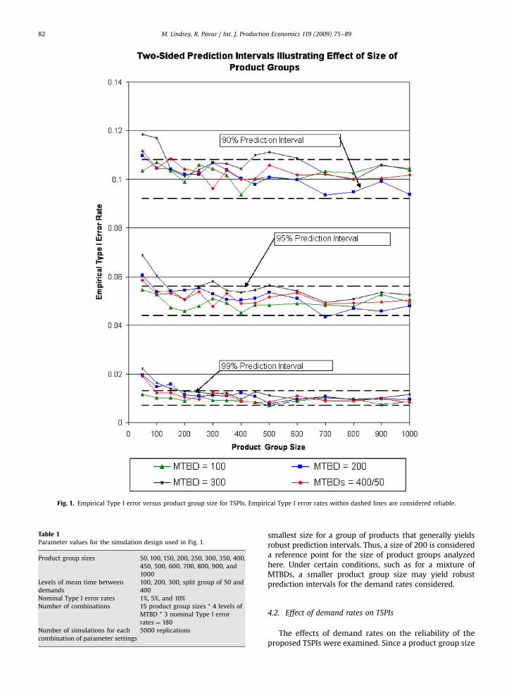
ARTICLE IN PRESS

Fig. 1. Empirical Type I error versus product group size for TSPIs. Empirical Type I error rates within dashed lines are considered reliable.

Table 1Parameter values for the simulation design used in Fig. 1.

Product group sizes 50, 100, 150, 200, 250, 300, 350, 400,

450, 500, 600, 700, 800, 900, and

1000

Levels of mean time between

demands

100, 200, 300, split group of 50 and

400

Nominal Type I error rates 1%, 5%, and 10%

Number of combinations 15 product group sizes * 4 levels of

MTBD * 3 nominal Type I error

rates ¼ 180

Number of simulations for each

combination of parameter settings

5000 replications


smallest size for a group of products that generally yieldsrobust prediction intervals. Thus, a size of 200 is considereda reference point for the size of product groups analyzedhere. Under certain conditions, such as for a mixture ofMTBDs, a smaller product group size may yield robustprediction intervals for the demand rates considered.

4.2. Effect of demand rates on TSPIs

The effects of demand rates on the reliability of theproposed TSPIs were examined. Since a product group size

ARTICLE IN PRESS

Table 2Empirical Type I error for TSPIs in Fig. 1.

Number of products 90% TSPI with MTBD ¼ 100 90% TSPI with MTBD ¼ 200 90% TSPI with MTBD ¼ 300 90% TSPI with MTBDs ¼ 400/50

50 0.103 0.110* 0.118* 0.112*

100 0.107 0.105 0.117* 0.105

150 0.103 0.104 0.104 0.108*

200 0.099 0.102 0.101 0.104

250 0.106 0.102 0.104 0.103

300 0.104 0.107 0.107 0.096

350 0.102 0.104 0.106 0.104

400 0.094 0.100 0.104 0.100

450 0.100 0.098 0.110* 0.100

500 0.101 0.109 0.111* 0.106

600 0.100 0.100 0.109* 0.102

700 0.103 0.094 0.102 0.102

800 0.103 0.095 0.100 0.100

900 0.106 0.099 0.106 0.100

1000 0.104 0.094 0.104 0.102


50 0.055 0.061* 0.069* 0.058*

100 0.052 0.054 0.060* 0.053

150 0.047 0.054 0.054 0.053

200 0.046 0.054 0.051 0.051

250 0.048 0.055 0.056 0.054

300 0.051 0.053 0.058* 0.048

350 0.049 0.051 0.054 0.053

400 0.045 0.050 0.054 0.049

450 0.048 0.051 0.057* 0.049

500 0.048 0.054 0.056 0.052

600 0.049 0.051 0.054 0.053

700 0.048 0.043* 0.049 0.049

800 0.048 0.047 0.051 0.049

900 0.053 0.046 0.054 0.050

1000 0.050 0.048 0.052 0.050


50 0.012 0.020* 0.022* 0.019*

100 0.010 0.015* 0.016* 0.012

150 0.010 0.016* 0.014* 0.012

200 0.009 0.011 0.013 0.010

250 0.011 0.011 0.012 0.010

300 0.009 0.011 0.012 0.013

350 0.009 0.011 0.012 0.011

400 0.009 0.012 0.010 0.010

450 0.008 0.011 0.013 0.008

500 0.007* 0.008 0.011 0.009

600 0.009 0.010 0.010 0.011

700 0.010 0.011 0.010 0.009

800 0.010 0.009 0.010 0.009

900 0.007* 0.010 0.010 0.010

1000 0.009 0.010 0.012 0.008

*Indicate TSPIs that are not reliable.


of 200 is considered a reference point as mentionedpreviously, a group of 200 products was used in furtheranalysis in which MTBDs ranging from 15 to 1000, asshown on the horizontal axis of Fig. 2, were used toexamine the reliability of the TSPIs. Fig. 2 reveals that theprediction intervals’ empirical Type I errors are higherwhen the demand rate is relatively high (relatively shortMTBD) or the demand rate is relatively low (relativelylong MTBD). The 90% and 95% TSPIs have confidence levelsclose to their respective 90% and 95% nominal levels for

MTBDs as high as 800. The 99% TSPIs are reliable forMTBDs between 30 and 300. The simulations suggest thatthe empirical Type I error rates are close to the nominalType I error for the underlying MTBD between 15 toaround 100, but then are less close as the MTBD increasestoward 1,000 at which point the TSPIs are no longerreliable.

Not every possible interval in the range investigatedwas examined. For faster moving products, changes inthe MTBD resulted in more substantial changes in the

ARTICLE IN PRESS

Fig. 2. Empirical Type I error versus MTBD for TSPI for 200 products. Empirical Type I error rates within dashed lines are considered reliable.


empirical Type I error rates of the TSPIs than for largerMTBDs so additional simulations were conducted in thatrange. Again, to keep the total number of simulations at areasonable level, values for MTBD were selected so thatmore simulations were conducted at MTBDs that were nottoo extreme.

A possible explanation for the results illustrated inFig. 2 is that the TSPIs have empirical Type I errors closerto their nominal value when there are a sufficient numberof products with no sales and a sufficient number ofproducts with some sales. When demand is high (shortMTBD), few periods with no sales exist. As the demanddecreases too much, many periods of zero demand exist,resulting in few products with observed sales. As

expected, the 99% TSPI is more reliable over a smallerrange of MTBDs than the 90% and 95% TSPIs.

5. Discussion and implications

Our research addressed the problem of estimatingfuture demand rates for products having a low demandrate. A new methodology adapted from software relia-bility models was investigated in a simulation studyacross a variety of experimental conditions includingproduct group size, MTBDs and Type I error levels.The lower and upper bounds of these proposed predictionintervals may be used by managers to make critical

ARTICLE IN PRESS


decisions about slow-moving products. For example, theupper bound on the demand rate from the TSPI can bemultiplied by the average price of the products displayingno demand over a fixed time period to obtain an estimateof the maximum rate of revenue in the future. If themaximum rate of revenue is too small to make theproducts worth holding, then a decision may be made toliquidate these products. The lower bound from the TSPImultiplied by the average product’s price provides anestimate of the minimum revenue. If a retailer must carrythese products out of necessity, then this value providesan estimate of the minimum revenue rate that a retailercan expect in the future. An inventory manager should usethe proposed prediction intervals as only one sourceof input in the decision making process of inventorymanagement. For example, an inventory manager mayhave expert knowledge about the demand of certainproducts or might know that the demand was high forcertain products before the observed period started. Thus,the manager should use all knowledge, including theresults of the proposed prediction intervals, in making afinal determination about stocking each product.

The purpose of this simulation study was to determineconditions under which the proposed prediction intervalswere reliable. The proposed prediction intervals werereferred to as being robust if they maintain their nominalconfidence level under changing conditions. The proposedprediction intervals were generally robust for productgroup sizes of 200 or more. Furthermore, an implicitassumption was that product demand was observed for100 time units. For this study, a time frame of 100 timeunits was selected as it provided sufficient time to observedemand using various underlying values for the demandrates in the simulation study. The choice of 100 time unitsis a limitation to this study for applications where a timeunit larger than a month would be required. For managersinterested in a different number of units for the timeframe, the simulation could be repeated for that value.

The results of this simulation study support theproposed prediction intervals as viable methodology togain insight into a range of likely values for the futuredemand rate of products with observed demand of zero.Under basic assumptions of a Poisson process for demandand independence of product demand, the predictionintervals are robust when the size of the group of productsis large with a sizable number of slow-moving products.As illustrated by the histogram in Fig. 3 with a productgroup size of 200 and an MTBD of 300, the normaldistribution is a good approximation for the distributionof M1ðtÞ=t. The results in Figs. 1 and 2 support robustperformance of the prediction intervals over a wide rangeof parameters.

A natural question that arises is ‘‘What are thethreshold values for the TSPIs to be robust with respectto product mix, product group size, demand rate, and timeframe?’’ Exact answers would require a rather extensivesimulation study. General guidelines and thoughts areprovided in the remainder of this section.

With respect to the time frame parameter, managersmay have some control over the length of time to observedemand before constructing TSPIs. The TSPIs should be

constructed for products displaying zero demand becausethe time frame over which demand is observed is notsufficiently long to observe the true demand rate of theproducts. If long enough time periods were selected thenthere would be few, if any, products with zero demand. Inthat case, traditional estimation would be fairly accuratesince most of the products would yield sufficient demandinformation. Through experimentation, the authors havefound that a sufficient threshold for the time frameparameter should be a value in which most of theproducts have exhibited at least one demand. Withrespect to the mixture parameter, the exact mixtureof slow-moving and fast-moving products does not appearto impact the performance of the TSPIs as much as thesample size of the product group. The next two para-graphs will address how and why the demand rate(MTBD) and product group size impact the performanceof the proposed prediction intervals. The last paragraph ofthis section explains that a violation of the underlyingassumptions used of the proposed methodology mayimpact the performance of the TSPIs. With these caveats,inventory managers may find the proposed predictionintervals to be an important source of information in thedecision process of maintaining inventory levels.

How and why are TSPIs affected by products that areselling too fast or too slow? As previously mentioned, if allproducts sell too fast or hardly at all, the TSPIs are notrobust. Thus, the demand rate plays an important rolein the proposed prediction intervals being reliable.The MTBD, which is the inverse of the demand rate, wasvaried to study the robustness of the proposed predictionintervals. If the MTBD was less than 20, that is, on averagea sale occurs sooner than every 20 time periods, proposedprediction intervals were not reliable. In other words, ifproducts were selling too fast, then the proposed predic-tion intervals will not be meaningful. The reason that theprediction intervals would not be meaningful is becausethe number of products with zero demand or evena demand of one unit of a product would be small.As illustrated by the histogram in Fig. 3 with a productgroup size of 50, the normal distribution is not a goodapproximation to the distribution of the demand ratewhen most products sell quickly and that poor approx-imation may make the empirical confidence level toosmall. Although prediction intervals on the future demandof products provide additional information in makingdecisions about safety levels of inventory (Shenstone andHyndman, 2005; Hong et al., 2008), this methodologyshould not be used in decision making about inventorylevels when the number of slow-moving products aresmall. However in the case of few slow-moving products,prediction intervals for the group of products usingtraditional estimation would be fairly accurate since mostof the products will yield sufficient demand informationover a reasonably specified time frame. As shown in thesimulation study, a proposed 90% prediction interval wasreliable for MTBDs ranging between 30 and 800 timeunits. At the 95% and 99% confidence levels, the necessaryMTBDs were between 20 and 800 time units and be-tween 30 and 300 time units, respectively. Products witha very small demand, for example, an MTBD in excess of

ARTICLE IN PRESS

0.0450

5

10

15

20

25

0.30

2.5

5.0

7.5

10.0

12.5

15.0

17.5

20.0

22.5

Per

cent

Per

cent

Empirical Rate

Empirical Rate0.06 0.075 0.09 0.105 0.12 0.135 0.15 0.165 0.18 0.195 0.21

0.33 0.36 0.39 0.42 0.45 0.48 0.51 0.54 0.57 0.6 0.63 0.66

Fig. 3. Distribution of 50 products over 100 time periods with MTBD of 300 and distribution of 200 products over 100 time periods with MTBD of 300.


800 time units, will be occurring too infrequently toprovide enough information to construct proposed pre-diction intervals that are reliable.

How and why are TSPIs affected by the size of theproduct groups? As previously mentioned, too fewproducts (small sample size) do not provide sufficientdata to obtain accurate estimates of the demand rate or itsvariation. Increasing the number of products resulted inimproved reliabilities for the proposed prediction inter-vals. The histograms in Fig. 3 clearly illustrate that a smallproduct group size results in the normal distribution notbeing a good approximation of the distribution of M1ðtÞ=t.Since the product group size of 200 did not providereliable prediction intervals for a number of MTBDs,especially large MTBDs, an additional study was con-ducted using a product group size of 600. Table 3summarizes the results. An R and a U denote whetherthe proposed prediction interval was reliable (R) or

unreliable (U), respectively. Interestingly, the largerproduct group size did not result in a substantial improve-ment in reliability. A possible explanation was that thereare MTBD levels at which demand is too low to obtainsufficient demand to provide reliable prediction intervalsregardless of the size of the product group. Thus, alarge sample size is needed, but as in most statisticalmethodology, there is little return for huge sample sizes asTable 3 illustrates.

How and why are TSPIs affected by violations of theunderlying assumptions? If the demand for productsdoes not follow a Poisson process, the proposed predictionintervals may not be reliable, i.e., the empirical confidencelevel may be much lower than the nominal level. Asin most statistical methodology, the distribution of thedata may easily affect the resulting distribution of theestimators. The normal approximation used in developingthe prediction intervals may be poor for data with lumpy

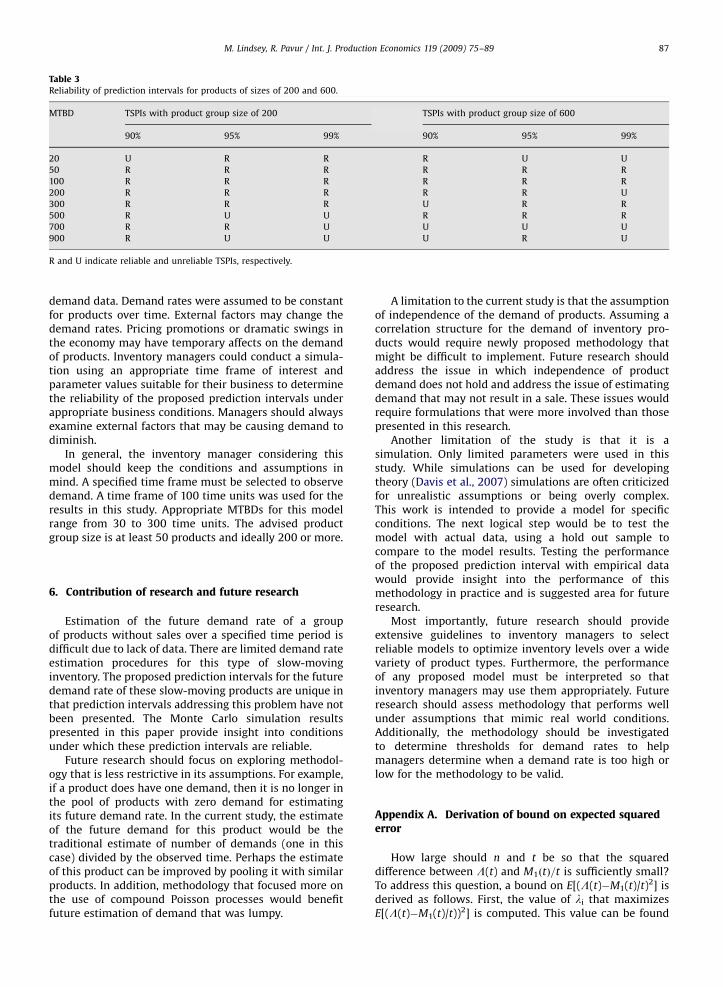
ARTICLE IN PRESS

Table 3Reliability of prediction intervals for products of sizes of 200 and 600.

MTBD TSPIs with product group size of 200 TSPIs with product group size of 600

90% 95% 99% 90% 95% 99%

20 U R R R U U

50 R R R R R R

100 R R R R R R

200 R R R R R U

300 R R R U R R

500 R U U R R R

700 R R U U U U

900 R U U U R U

R and U indicate reliable and unreliable TSPIs, respectively.


demand data. Demand rates were assumed to be constantfor products over time. External factors may change thedemand rates. Pricing promotions or dramatic swings inthe economy may have temporary affects on the demandof products. Inventory managers could conduct a simula-tion using an appropriate time frame of interest andparameter values suitable for their business to determinethe reliability of the proposed prediction intervals underappropriate business conditions. Managers should alwaysexamine external factors that may be causing demand todiminish.

In general, the inventory manager considering thismodel should keep the conditions and assumptions inmind. A specified time frame must be selected to observedemand. A time frame of 100 time units was used for theresults in this study. Appropriate MTBDs for this modelrange from 30 to 300 time units. The advised productgroup size is at least 50 products and ideally 200 or more.

6. Contribution of research and future research

Estimation of the future demand rate of a groupof products without sales over a specified time period isdifficult due to lack of data. There are limited demand rateestimation procedures for this type of slow-movinginventory. The proposed prediction intervals for the futuredemand rate of these slow-moving products are unique inthat prediction intervals addressing this problem have notbeen presented. The Monte Carlo simulation resultspresented in this paper provide insight into conditionsunder which these prediction intervals are reliable.

Future research should focus on exploring methodol-ogy that is less restrictive in its assumptions. For example,if a product does have one demand, then it is no longer inthe pool of products with zero demand for estimatingits future demand rate. In the current study, the estimateof the future demand for this product would be thetraditional estimate of number of demands (one in thiscase) divided by the observed time. Perhaps the estimateof this product can be improved by pooling it with similarproducts. In addition, methodology that focused more onthe use of compound Poisson processes would benefitfuture estimation of demand that was lumpy.

A limitation to the current study is that the assumptionof independence of the demand of products. Assuming acorrelation structure for the demand of inventory pro-ducts would require newly proposed methodology thatmight be difficult to implement. Future research shouldaddress the issue in which independence of productdemand does not hold and address the issue of estimatingdemand that may not result in a sale. These issues wouldrequire formulations that were more involved than thosepresented in this research.

Another limitation of the study is that it is asimulation. Only limited parameters were used in thisstudy. While simulations can be used for developingtheory (Davis et al., 2007) simulations are often criticizedfor unrealistic assumptions or being overly complex.This work is intended to provide a model for specificconditions. The next logical step would be to test themodel with actual data, using a hold out sample tocompare to the model results. Testing the performanceof the proposed prediction interval with empirical datawould provide insight into the performance of thismethodology in practice and is suggested area for futureresearch.

Most importantly, future research should provideextensive guidelines to inventory managers to selectreliable models to optimize inventory levels over a widevariety of product types. Furthermore, the performanceof any proposed model must be interpreted so thatinventory managers may use them appropriately. Futureresearch should assess methodology that performs wellunder assumptions that mimic real world conditions.Additionally, the methodology should be investigatedto determine thresholds for demand rates to helpmanagers determine when a demand rate is too high orlow for the methodology to be valid.

Appendix A. Derivation of bound on expected squarederror

How large should n and t be so that the squareddifference between L(t) and M1ðtÞ=t is sufficiently small?To address this question, a bound on E[(L(t)�M1(t)/t)2] isderived as follows. First, the value of li that maximizesE[(L(t)�M1(t)/t))2] is computed. This value can be found

ARTICLE IN PRESS


by finding the maximum of the function f(li) presentedbelow.

f ðliÞ ¼l2

i þ li

t

!e�lit ; i ¼ 1;2;3; . . . ;n

To find the max of f ðliÞ, df ðliÞ=dli ¼ 0.

2li þ 1

t

� �e�lit þ

l2i þ li

t

!ð�tÞe�li t ¼ 0

Therefore, tli2+(t�2)li�1 ¼ 0 and

E LðtÞ �M1ðtÞ

t

� �2" #

¼Xn

i¼1

l2i þ li

t

!e�li tp

Xn

i¼1

2�tþffiffiffiffiffiffiffiffit2þ4p

2t

� �2

þ2�tþ

ffiffiffiffiffiffiffiffit2þ4p

2t

t

0BBB@

1CCCAe�ð2�tþ


=2tÞt

¼Xn

i¼1

4�2tþt2þ4ffiffiffiffiffiffiffiffit2þ4p

�2tffiffiffiffiffiffiffiffit2þ4p

þt2þ4þ4t�2t2þ2tffiffiffiffiffiffiffiffit2þ4p

4t2

� �t

0BB@

1CCAe�ð2�tþ


=2tÞt

¼n

t2

ðt þ 2ffiffiffiffiffiffiffiffiffiffiffiffiffit2 þ 4

pþ 4Þ

2te�2�tþ


=2p1:07n

t2assuming tX2.

li ¼2� t þ


p2t

i ¼ 1,2,y,n. Now, the second derivative is presented.

d2f ðliÞ

dl2i

¼2

te�li t � t

2li þ 1

te�lit � ð2li þ 1Þe�lit

þ tðl2i þ liÞe

�li t

d2f ðliÞ

dl2i

¼ e�li t2

tþ tl2

i þ ðt � 4Þli � 2

The second derivative evaluated at

li ¼2� t þ


p2t

is

d2f ðliÞ

dl2i

¼ e�li t2

tþ t

2� t þffiffiffiffiffiffiffiffiffiffiffiffiffit2 þ 4

p2t

!224

þ ðt � 4Þ2� t þ


p2t

!� 2

#

¼ e�li t2

tþ

4� 4t þ t2 þ 2ð2� tÞffiffiffiffiffiffiffiffiffiffiffiffiffit2 þ 4

pþ t2 þ 4

4t

"

þ2t � t2 � 8þ 4t þ t


p� 4


p2t

� 2

#

¼ e�li t2

tþ

4� 2t þ t2 þ 2ffiffiffiffiffiffiffiffiffiffiffiffiffit2 þ 4

p� t


p2t

"

þ6t � t2 � 8þ t


p� 4


p2t

� 2

#

¼ e�lit �


pt

" #

The expected squared difference E½ðLðtÞ �M1ðtÞ=tÞ2� ismaximized at

li ¼2� t þ


p2t

i ¼ 1;2; . . .n.

For tX2, a bound for this expression is established.

Inequality above follows by noting that e�ð2�tþffiffiffiffiffiffiffiffit2þ4p

=2Þ isan increasing function in t with an upper bound of e�1 and

that t þ 2ffiffiffiffiffiffiffiffiffiffiffiffiffit2 þ 4

pþ 4=2t is a decreasing function in t.

The value of 1.07 is equal to the product of e�1 and the

expression t þ 2ffiffiffiffiffiffiffiffiffiffiffiffiffit2 þ 4

pþ 4=2t evaluated at t ¼ 2.

References

Altay, N., Rudisill, F., Litteral, L.A., 2008. Adapting Wright’s modificationof Holt’s method to forecasting intermittent demand. InternationalJournal of Production Economics 111 (2), 389–408.

Abdel-ghaly, A.A., Chan, P.Y., Littlewood, B., 1986. Evaluation of compet-ing software reliability predictions. IEEE Transactions on SoftwareEngineering 12 (9), 950–967.

Bagchi, U., Hayya, J.C., Ord, J.K., 1983. The Hermite distribution as a modelof demand during lead time for slow-moving items. DecisionSciences 14 (4), 447–466.

Boylan, J.E., Syntetos, A.A., 2007. The accuracy of a modified Crostonprocedure. International Journal of Production Economics 107 (2),511–517.

Boylan, J.E., Syntetos, A.A., Karakostas, G.C., 2008. Classification forforecasting and stock control: a case study. Journal of the OperationalResearch Society 59 (4), 473–481.

Box, G.E.P., Jenkins, G.M., Reinsel, G.C., 1994. Time Series Analysis:Forecasting and Control, third ed. Prentice-Hall, Englewood Cliffs, NJ.

Brown Jr., G.F., Rogers, W.F., 1973. A Bayesian approach to demandestimation and inventory provisioning. Naval Research LogisticsQuarterly 20 (4), 607–624.

Burton, R.W., Jaquette, S.C., 1973. The initial provisioning decision forinsurance type items. Naval Research Logistics Quarterly 20 (1),123–146.

Caniato, F., Kalchschmidt, M., Ronchi, S., Verganti, R., Zotteri, G., 2005.Clustering customers to forecast demand. Production Planning andControl 16 (1), 32–43.

Chatfield, D.C., Hayya, J., 2007. All-zero forecasts for lumpy demand: afactorial study. International Journal of Production Research 45 (4),935–950.

Croston, J.D., 1972. Forecasting and stock control for intermittentdemands. Operational Research Quarterly 23 (3), 289–303.

Dalhart, G. 1974. Class seasonality—a new approach. In: Proceedings ofthe American Production and Inventory Control Society 1974Conference, second ed., APICS, Washington, DC, pp. 11–16. Reprintedin Forecasting.

ARTICLE IN PRESS


Davis, J.P., Eisenhardt, K.M., Bingham, C.B., 2007. Developing theorythrough simulation methods. The Academy of Management Review32 (2), 480–499.

Dekker, M., van Donselaar, K., Ouwehand, P., 2004. How to useaggregation and combined forecasting to improve seasonal demandforecasts. International Journal of Production Economics 90, 151–167.

Dolgui, A., Pashkevich, M., 2008. Demand forecasting for multiple slow-moving items with short requests history and unequal demandvariance. International Journal of Production Economics 112,885–894.

Gardner Jr., E.S., 2006. Exponential smoothing: the state of the art—partII. International Journal of Forecasting 22 (4), 637–666.

Gelders, L.F., Van Looy, P.M., 1978. An inventory policy for slow and fastmovers in a petrochemical plant: a case study. Journal of theOperational Research Society 29 (9), 867–874.

Haber, S.E., Sitgreaves, R., 1970. A methodology for estimating expectedusage of repair parts with application to parts with no usage history.Naval Research Logistics Quarterly 17 (4), 535–546.

Harwell, M.R., 1991. Using randomization tests when errors areunequally correlated. Computational Statistics and Data Analysis 11(1), 75–85.

Hong, J.S., Koo, H.-Y., Lee, C.-S., Ahn, J., 2008. Forecasting serviceparts demand for a discontinued product. IIE Transactions 40 (7),640–646.

Johnston, F.R., Boylan, J.E., 1996. Forecasting for items with intermittentdemand. Journal of the Operational Research Society 47 (1), 113–121.

Kaufman, G.M., 1996. Successive sampling and software reliability.Journal of Statistical Planning and Inference 49 (3), 343–369.

Leven, E., Segerstedt, A., 2004. Inventory control with a modified Crostonprocedure and Erlang distribution. International Journal of Produc-tion Economics 90 (3), 361–367.

Masters, J.M., 1993. Determination of near optimal stock levels for multi-echelon distribution inventories. Journal of Business Logistics 14 (2),165–195.

Miller, D.R., 1986. Exponential order statistic models of softwarereliability growth. IEEE Transactions on Software Engineering 12(1), 12–24.

Miragliotta, G., Staudacher, A.P., 2004. Exploiting information sharing,stock management and capacity over sizing in the management oflumpy demand. International Journal of Production Research 42 (13),2533–2554.

Muckstadt, J.A., Thomas, L.J., 1980. Are multi-echelon inventory methodsworth implementing in systems with low-demand-rate items?Management Science 26 (5), 483–494.

Ornek, A., Cengiz, O., 2006. Capacitated lot sizing with alternativeroutings and overtime decisions. International Journal of ProductionResearch 44 (24), 5363–5389.

Porras, E., Dekker, R., 2008. An inventory control system for spareparts at a refinery: an empirical comparison of different re-order

point methods. European Journal of Operational Research 184 (1),101–132.

Razi, M.A., Tarn, J.M., 2003. An applied model for improving inventorymanagement in ERP systems. Logistics Information Management 16(2), 114–124.

Ross, S.M., 1985a. Statistical estimation of software reliability. IEEETransactions on Software Engineering SE11 (5), 479–483.

Ross, S.M., 1985b. Software reliability: the stopping rule problem. IEEETransactions on Software Engineering SE11 (12), 1472–1476.

Ross, S.M., 2002. Introduction to Probability Models, sixth ed. AcademicPress, New York.

Sani, B., Kingsman, B.G., 1997. Selecting the best periodic inventorycontrol and demand forecasting methods for low demand items.Journal of the Operational Research Society 48 (7), 700–713.

Schultz, C.R., 1987. Forecasting and inventory control for sporadicdemand under periodic review. Journal of the Operational ResearchSociety 38 (5), 453–458.

Shenstone, L., Hyndman, R.J., 2005. Stochastic models underlyingCroston’s method for intermittent demand forecasting. Journal ofForecasting 24 (6), 389–402.

Silver, E.A., 1965. Bayesian determination of the reorder point of a slow-moving item. Operations Research 13 (6), 989–997.

Silver, E.A., 1970. Some ideas related to the inventory control of itemshaving erratic demand patterns. Journal of the Canadian OperationalResearch Society 8 (2), 87–100.

Smith, R., Vemuganti, R., 1969. A learning model for inventory control ofslow-moving items. AIIE Transactions 1, 274–277.

Syntetos, A.A., Boylan, J.E., 2001. On the bias of intermittent demandestimates. International Journal of Production Economics 71 (1–3),457–466.

Thompstone, R.M., Silver, E.A., 1975. A coordinated inventory controlsystem for compound Poisson demand and zero lead time. Interna-tional Journal of Production Research 13 (6), 581–602.

Vereecke, A., Verstraeten, P., 1994. An inventory management modelfor an inventory consisting of lumpy items, slow movers and fastmovers. International Journal of Production Economics 35 (1/3),379–389.

Willemain, T.R., Smart, C.N., Schwarz, H.F., 2004. A new approach toforecasting intermittent demand for service parts inventories.International Journal of Forecasting 20 (3), 375–387.

Willemain, T.R., Smart, C.N., Shockor, J.H., DeSautels, P.A., 1994.Forecasting intermittent demand in manufacturing: a comparativeevaluation of Croston’s method. International Journal of Forecasting10 (4), 529–538.

Williams, T.M., 1984. Stock control with sporadic and slow-movingdemand. Journal of the Operational Research Society 35 (10),939–948.

Zwick, R., 1986. Rank and normal scores alternatives to Hotelling’s T2.Multivariate Behavioural Research 21 (2), 169–186.

prediction intervals for future demand of existing products with an observed demand of zero

Documents