prediction in mlm
TRANSCRIPT

Prediction in MLMModel comparisons and regularization
PSYC 575
October 13, 2020 (updated: 25 October 2020)
Learning Objectives
• Describe the role of prediction in data analysis
• Describe the problem of overfitting when fitting complex models
• Use information criteria to compare models
• Use regularizing priors to increase the predictive accuracy of complex models

Prediction

Yarkoni & Westfall (2017)1
• “Psychology’s near-total focus on explaining the causes of behavior has led [to] … theories of psychological mechanism but … little ability to predict future behaviors with any appreciable accuracy” (p. 1100)
[1]: https://doi.org/10.1177/17456916176933
Prediction in Data Analysis
• Explanation: Students with higher SES receive higher quality of education prior to high school, so schools with higher MEANSES tends to perform better in math achievement
• Prediction: Based on the model, a student with an SES of 1 in a school with MEANSES = 1 is expected to score 18.5 on math achievement, with a prediction error of 2.5
Can We Do Explanation Without Prediction?
• “People in a negative mood were more aware of their physical symptoms, so they reported more symptoms.”
• And then . . .
• “Knowing that a person has a mood level of 2 on a given day, the person can report anywhere between 0 to 10 symptoms”
• Is this useful?
Can We Do Explanation Without Prediction?
• “CO2 emission is a cause of warmer global temperature.”
• And then . . .
• “Assuming that the global CO2 emission level in 2021 is 12 Bt, the global temperature in 2022 can change anywhere between -100 to 100 degrees”
• Is this useful?

Predictions in Quantitative Sciences
• It may not be the only goal of science, but it does play a role• Perhaps the most important goal in some research
• A theory that leads to no, poor, or imprecise predictions may not be useful
• Prediction does not require knowing the causal mechanism, but it requires more than binary decision of significance/non-significance
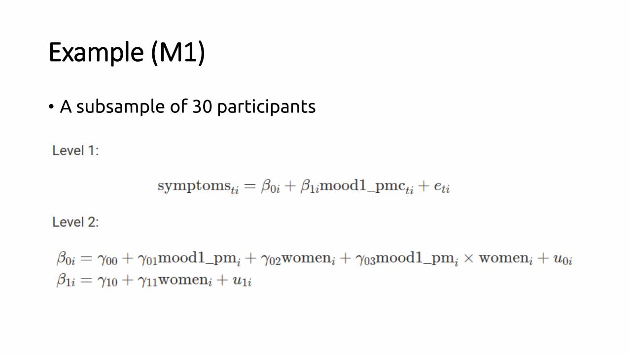
Example (M1)
• A subsample of 30 participants

Two Types of Predictions
• Cluster-specific: For a person (cluster) in the data set, what is the predicted symptom level when given the predictors (e.g., mood1, women) and the person- (cluster-)specific random effects (i.e., the u’s)
> (obs1 <- stress_data[1, c("PersonID", "mood1_pm", "mood1_pmc", "women")])
PersonID mood1_pm mood1_pmc women
1 103 0 0 women> predict(m1, newdata = obs)
Estimate Est.Error Q2.5 Q97.5
[1,] 0.3251539 0.8229498 -1.249965 1.966336
For person with ID 103, on a day with mood = 0, she is predicted to have 0.33 symptoms, with 95% prediction interval [-1.25, 1.97]
Two Types of Predictions
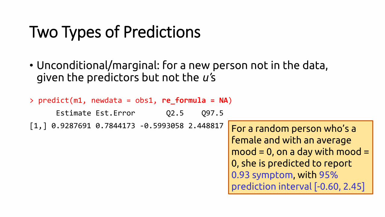
• Unconditional/marginal: for a new person not in the data, given the predictors but not the u’s
> predict(m1, newdata = obs1, re_formula = NA)
Estimate Est.Error Q2.5 Q97.5
[1,] 0.9287691 0.7844173 -0.5993058 2.448817 For a random person who’s a female and with an average mood = 0, on a day with mood = 0, she is predicted to report 0.93 symptom, with 95% prediction interval [-0.60, 2.45]
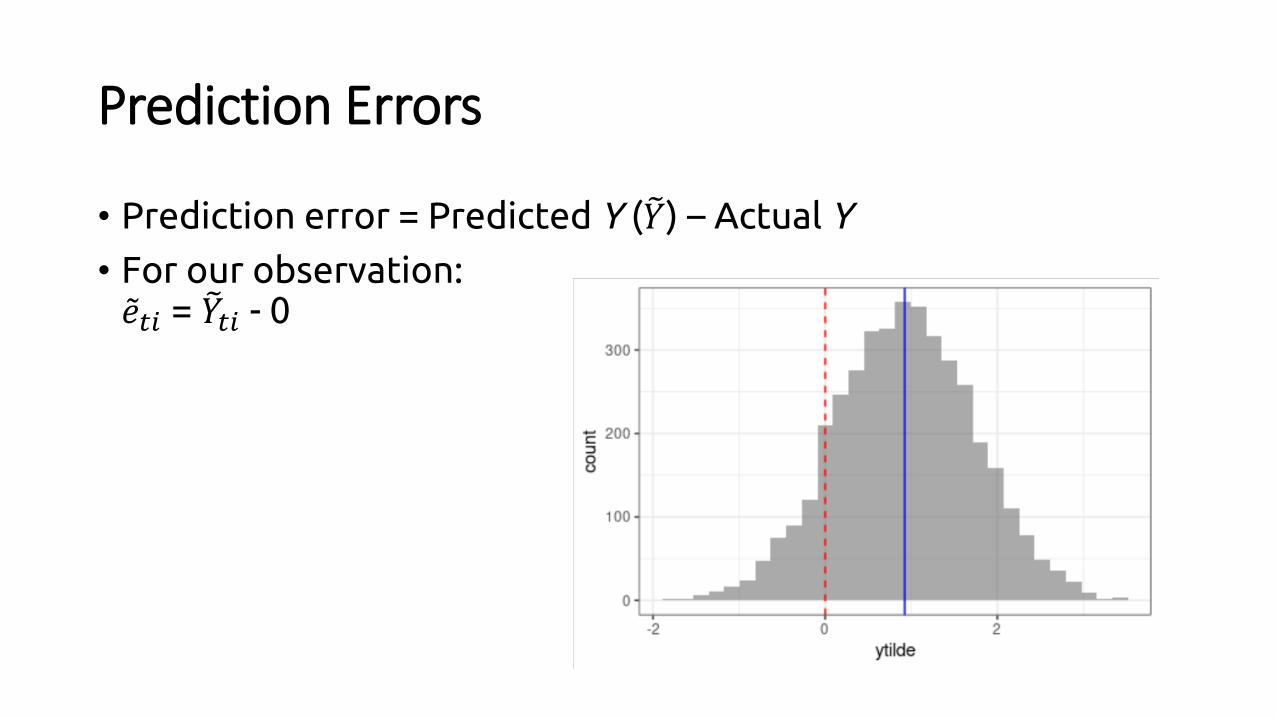
Prediction Errors
• Prediction error = Predicted Y ( ෨𝑌) – Actual Y
• For our observation:ǁ𝑒𝑡𝑖 = ෨𝑌𝑡𝑖 - 0

Average In-Sample Prediction Error
• Mean squared error (MSE): σσ ǁ𝑒𝑡𝑖2 /𝑁
• In-sample MSE: average squared prediction error when using the same data to build the model and compute prediction
• Here we have in-sample MSE = 1.04• The average squared prediction error is 1.04 symptoms

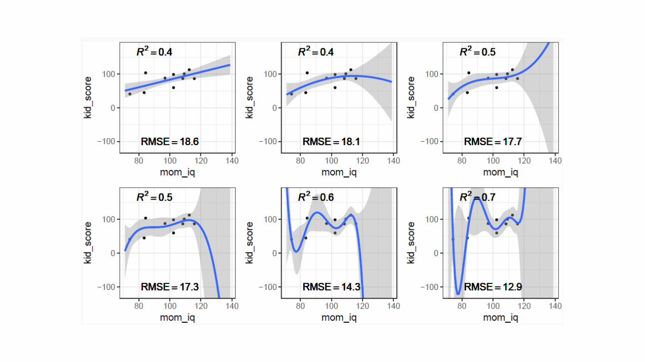
Overfitting
Overfitting
• When a model is complex enough, it will reproduce the data perfectly (i.e., in-sample MSE)
• It does so by capturing all idiosyncrasy (noise) of the data
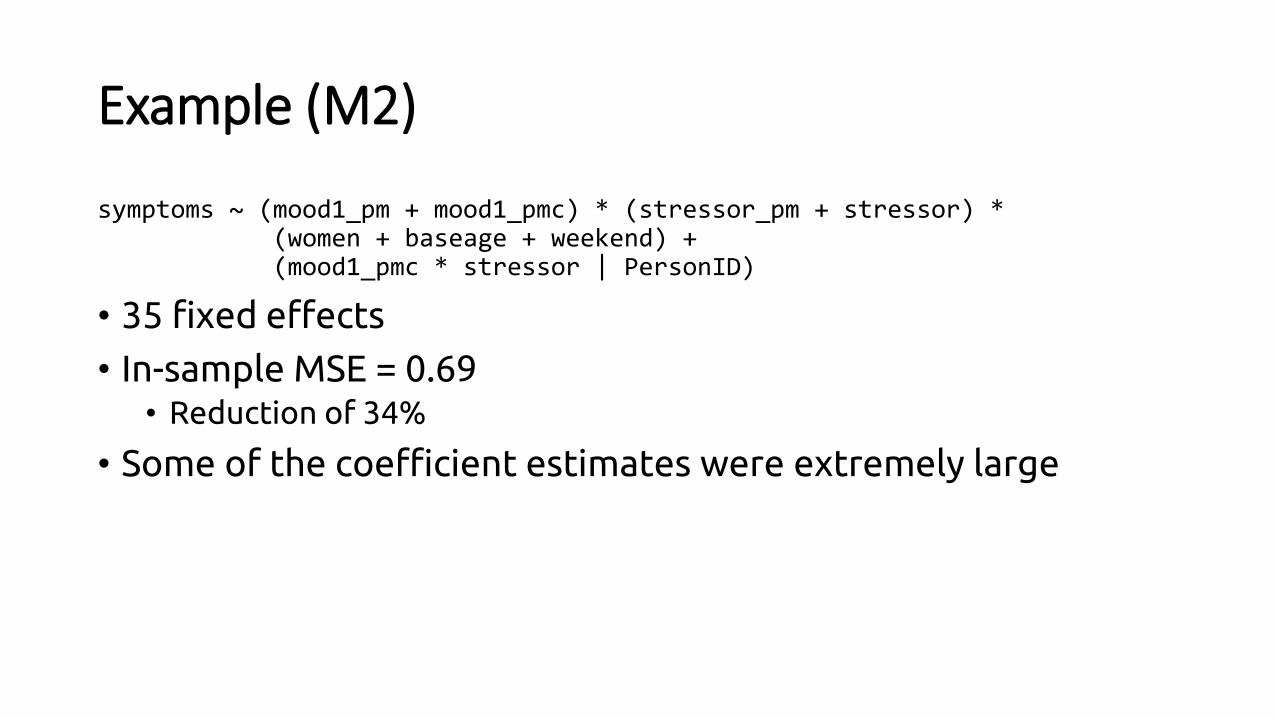
Example (M2)
symptoms ~ (mood1_pm + mood1_pmc) * (stressor_pm + stressor) * (women + baseage + weekend) + (mood1_pmc * stressor | PersonID)
• 35 fixed effects
• In-sample MSE = 0.69• Reduction of 34%
• Some of the coefficient estimates were extremely large
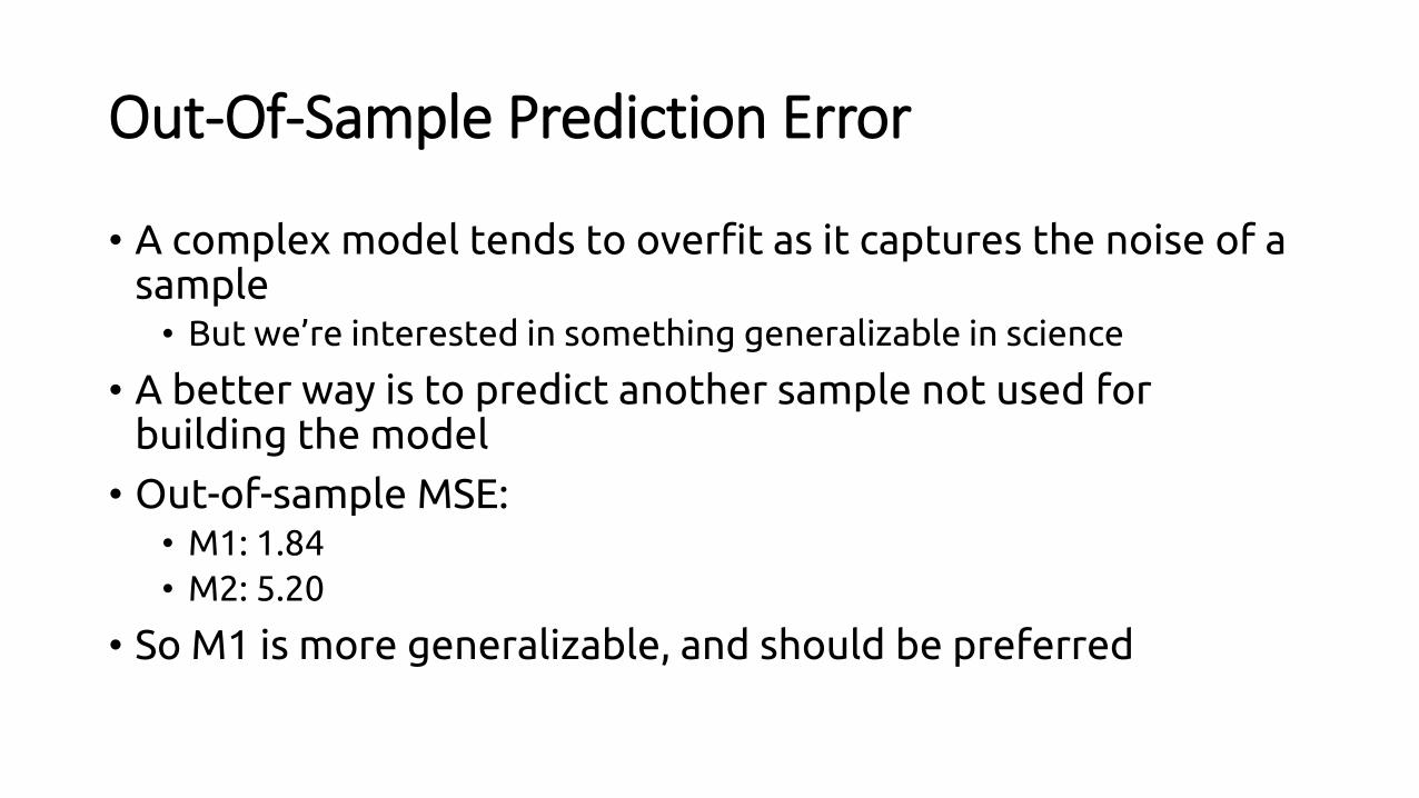
Out-Of-Sample Prediction Error
• A complex model tends to overfit as it captures the noise of a sample• But we’re interested in something generalizable in science
• A better way is to predict another sample not used for building the model
• Out-of-sample MSE:• M1: 1.84
• M2: 5.20
• So M1 is more generalizable, and should be preferred

Estimating Out-of-Sample Prediction Error
Approximating Out-Of-Sample Prediction Error
• But we usually don’t have the luxury of a validation sample
• Possible solutions• Cross-validation
• Information criteria
• They are basically the same thing; just with different approaches (brute-force and analytical)
K-fold Cross-Validation (CV)
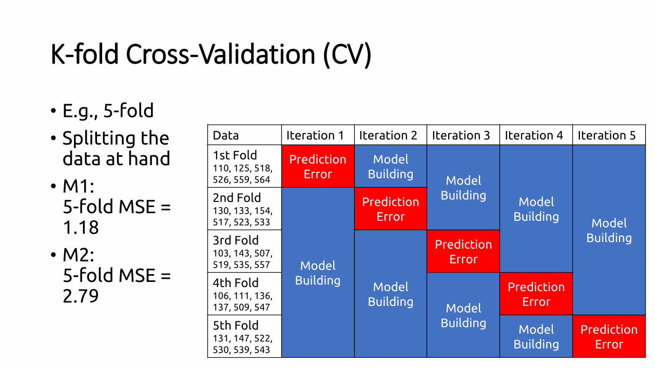
• E.g., 5-fold
• Splitting the data at hand
• M1: 5-fold MSE = 1.18
• M2:5-fold MSE = 2.79
Data Iteration 1 Iteration 2 Iteration 3 Iteration 4 Iteration 5
1st Fold110, 125, 518, 526, 559, 564
Prediction Error
Model Building
Model Building
Model Building
Model Building
2nd Fold130, 133, 154, 517, 523, 533
Model Building
Prediction Error
3rd Fold103, 143, 507,519, 535, 557
Model Building
Prediction Error
4th Fold106, 111, 136, 137, 509, 547 Model
Building
Prediction Error
5th Fold131, 147, 522, 530, 539, 543
Model Building
Prediction Error
Leave-One-Out (LOO) Cross Validation
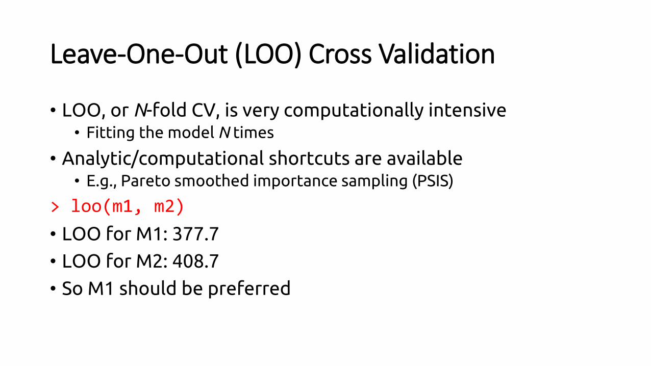
• LOO, or N-fold CV, is very computationally intensive• Fitting the model N times
• Analytic/computational shortcuts are available• E.g., Pareto smoothed importance sampling (PSIS)
> loo(m1, m2)
• LOO for M1: 377.7
• LOO for M2: 408.7
• So M1 should be preferred
Information Criteria
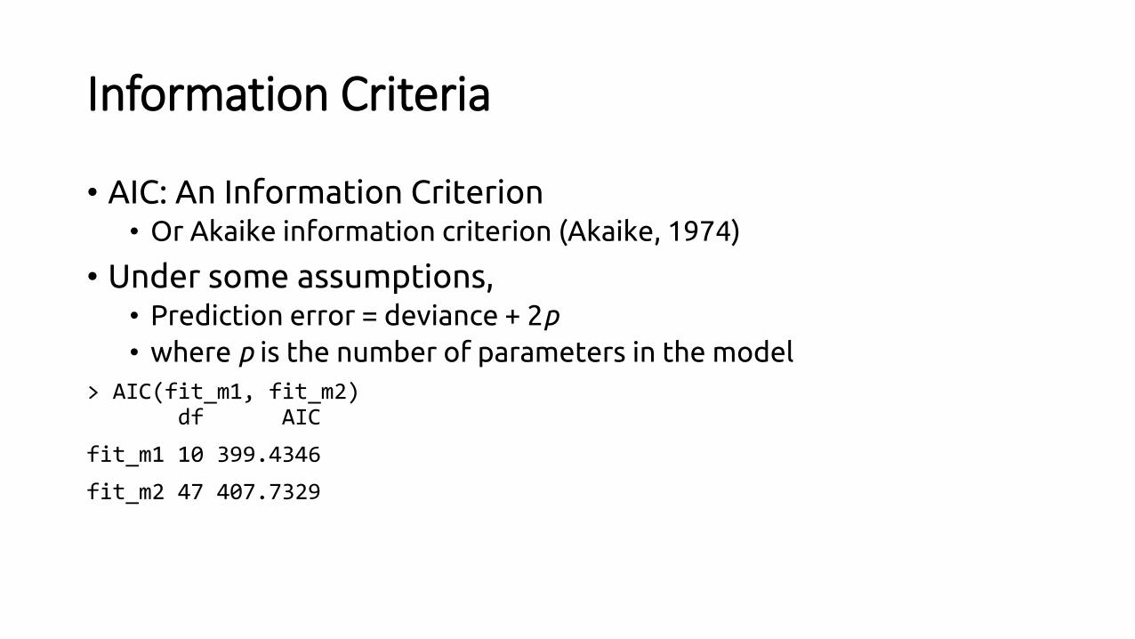
• AIC: An Information Criterion• Or Akaike information criterion (Akaike, 1974)
• Under some assumptions, • Prediction error = deviance + 2p
• where p is the number of parameters in the model
> AIC(fit_m1, fit_m2)df AIC
fit_m1 10 399.4346
fit_m2 47 407.7329

Information Criterion
• LOO in brms has a similar metric as the AIC, so it’s also called LOOIC
• LOO also approximates the complexity of the model (i.e., effective number of parameters)
> loo(m1)Estimate SE
elpd_loo -188.9 16.0p_loo 31.5 6.5Looic 377.7 32.1
> loo(m2)Estimate SE
elpd_loo -204.4 14.5p_loo 53.2 7.8Looic 408.7 29.0
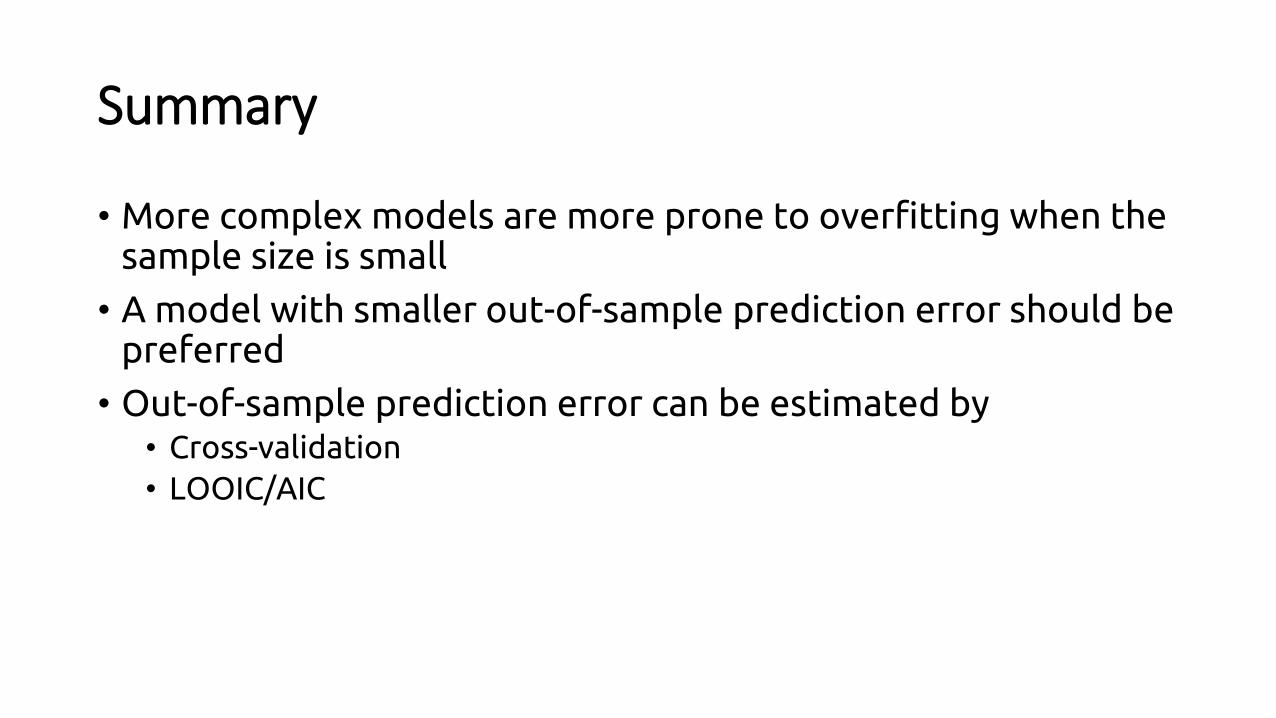
Summary
• More complex models are more prone to overfitting when the sample size is small
• A model with smaller out-of-sample prediction error should be preferred
• Out-of-sample prediction error can be estimated by• Cross-validation
• LOOIC/AIC

Regularization
Restrain a Complex Model From Learning Too Much
• Reduce overfitting by allowing each coefficient to only be partly based on the data
• The same idea as borrowing information in MLM• Empirical Bayes estimates of the group means are regularized
estimates
Regularizing Priors
• E.g., Lasso, ridge, etc
• A state-of-the-art method is the regularized horseshoe priors (Piironen & Vehtari, 2017)1
• Useful for variable selections when the number of predictors is large
• Because we need to compare predictors, the variables should be standardized (i.e., converted to Z scores)
• Let’s try on the full sample
[1]: https://projecteuclid.org/euclid.ejs/1513306866
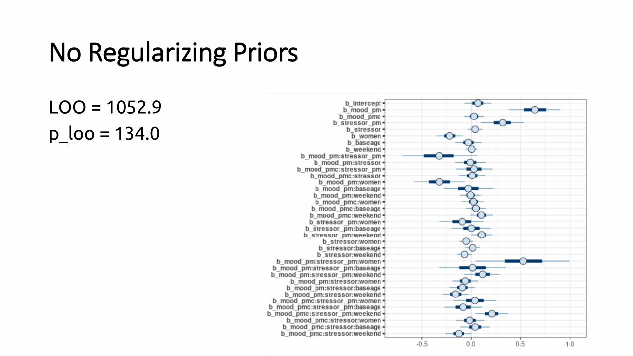
No Regularizing Priors
LOO = 1052.9
p_loo = 134.0
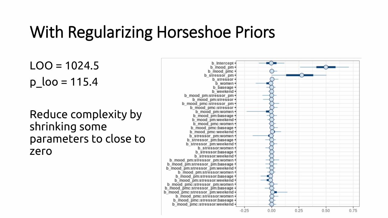
With Regularizing Horseshoe Priors
LOO = 1024.5
p_loo = 115.4
Reduce complexity byshrinking some parameters to close to zero
Summary
• Prediction error is a useful metric to gauge the performance of a model
• A complex model (with many parameters) is prone to overfitting when the sample size is small
• Models with lower LOOIC/AIC should be preferred as they tend to have lower out-of-sample prediction error
• Regularizing priors can be used to reduce model complexity and to promote better out-of-sample predictions
Topics Not Covered
• Other information criteria (e.g., mAIC/cAIC, BIC, etc)
• Classical regularization techniques (e.g., Lasso, ridge regression)
• Variable selection methods (see the projpred package)
• Model averaging