Prediction and Power inMolecular Sensors: Uncertaintyand Dissipation WhenConditionally MarkovianChannels are Driven by Semi-Markov EnvironmentsSarah E. MarzenJames P. Crutchfield

SFI WORKING PAPER: 2017-07-020

SFIWorkingPaperscontainaccountsofscienti5icworkoftheauthor(s)anddonotnecessarilyrepresenttheviewsoftheSantaFeInstitute.Weacceptpapersintendedforpublicationinpeer-reviewedjournalsorproceedingsvolumes,butnotpapersthathavealreadyappearedinprint.Exceptforpapersbyourexternalfaculty,papersmustbebasedonworkdoneatSFI,inspiredbyaninvitedvisittoorcollaborationatSFI,orfundedbyanSFIgrant.

©NOTICE:Thisworkingpaperisincludedbypermissionofthecontributingauthor(s)asameanstoensuretimelydistributionofthescholarlyandtechnicalworkonanon-commercialbasis.Copyrightandallrightsthereinaremaintainedbytheauthor(s).Itisunderstoodthatallpersonscopyingthisinformationwilladheretothetermsandconstraintsinvokedbyeachauthor'scopyright.Theseworksmayberepostedonlywiththeexplicitpermissionofthecopyrightholder.

www.santafe.edu

SANTA FE INSTITUTE

Santa Fe Institute Working Paper 2017-07-XXXarxiv.org:1707.03962 [physics.gen-ph]

Prediction and Power in Molecular Sensors:

Uncertainty and Dissipation When Conditionally Markovian ChannelsAre Driven by Semi-Markov Environments

Sarah E. Marzen1, ∗ and James P. Crutchfield2, †

1Physics of Living Systems, Department of Physics,Massachusetts Institute of Technology, Cambridge, MA 02139

2Complexity Sciences Center and Department of Physics,University of California at Davis, One Shields Avenue, Davis, CA 95616

(Dated: July 13, 2017)

Sensors often serve at least two purposes: predicting their input and minimizing dissipated heat.However, determining whether or not a particular sensor is evolved or designed to be accurate andefficient is difficult. This arises partly from the functional constraints being at cross purposes andpartly since quantifying the predictive performance of even in silico sensors can require prohibitivelylong simulations. To circumvent these difficulties, we develop expressions for the predictive accuracyand thermodynamic costs of the broad class of conditionally Markovian sensors subject to unifilarhidden semi-Markov (memoryful) environmental inputs. Predictive metrics include the instanta-neous memory and the mutual information between present sensor state and input future, whiledissipative metrics include power consumption and the nonpredictive information rate. Success inderiving these formulae relies heavily on identifying the environment’s causal states, the input’sminimal sufficient statistics for prediction. Using these formulae, we study the simplest nontriv-ial biological sensor model—that of a Hill molecule, characterized by the number of ligands thatbind simultaneously, the sensor’s cooperativity. When energetic rewards are proportional to totalpredictable information, the closest cooperativity that optimizes the total energy budget generallydepends on the environment’s past hysteretically. In this way, the sensor gains robustness to en-vironmental fluctuations. Given the simplicity of the Hill molecule, such hysteresis will likely befound in more complex predictive sensors as well. That is, adaptations that only locally optimizebiochemical parameters for prediction and dissipation can lead to sensors that “remember” the pastenvironment.

PACS numbers: 02.50.-r 89.70.+c 05.45.Tp 02.50.EyKeywords: predictive information rate, information processing, nonequilibrium steady state, thermodynamics

Introduction To perform functional tasks, synthetic

nanoscale machines and their macromolecular cousins si-

multaneously manipulate energy, information, and mat-

ter. They are information engines—systems that oper-

ate by synergistically balancing the energetics of their

physical substrate against required information genera-

tion, storage, loss, and transformation to support a given

functionality. Classically, information engines were con-

ceived as either potential computers [1]—that is, physi-

cal systems that can compute anything given the right

program—or as Maxwellian-like demons that use infor-

mation as a resource to convert disordered energy to use-

ful work [2–5]. Recently, investigations into functional

computation [6] embedded in physical systems led to

studies of the thermodynamics of various kinds of in-

formation processing [7], including the thermodynamic

costs of information creation [8], noise suppression [9],

error correction and synchronization [10], prediction [11–

∗ semarzen@mit.edu† chaos@ucdavis.edu

13], homeostasis [14], learning [15], structure [16], and

intelligent control [17].

Due to its broad importance to the survival of bio-

logical organisms, here we focus on a specific functional

computation in information engines: how sensory sub-

systems predict their environment. And, we introduce a

thermodynamic analysis that can address environmental

processes more complex than the memoryless and finite-

state Markov sources and Gaussian processes considered

in the above cited works.

Evolved and designed sensory systems are often tasked

with at least two, potentially competing, objectives: ac-

curately predicting inputs [18, 19] and minimizing re-

quired power and heat dissipation [20, 21] [22]. Accu-

rate and energy-efficient predictive models can be used

to optimize action policies, for example, to reap increased

rewards from the environment, even regardless of one’s

particular “reward function” [23–26].

Extracting such models from actual biological sensors

requires a nontrivial matching of sensory statistics and

sensor structure [14, 27]. Undaunted, much effort has

been invested to find minimally dissipative and maxi-

2

mally predictive sensors, often simplifying the challenges

by ignoring action policies—how the sensed information

is used. Some seek sensor models that maximize a combi-

nation of predictive power and (energetic) efficiency; e.g.

as in Refs. [12, 27]. Others validate learning rules based

on whether or not they maximize the aforementioned ob-

jective function [28, 29]. Finally, others compare real bi-

ological sensors to in silico null models; e.g. as in Ref.

[19].

These efforts require calculating predictive and dissi-

pative metrics of sensory models. For realistic null mod-

els, estimating predictive power from simulation can re-

quire prohibitively long simulations. To circumvent these

and related difficulties, then, one desires closed-form ex-

pressions for various predictive and dissipative metrics

in terms of the generators of environment behavior and

of the sensor-channel properties—the input-dependent

stochastic dynamical system describing the sensor. The

following provides these expressions for quite general sen-

sors: conditionally Markovian channels subject to com-

plex nonequilibrium steady-state environments that are

unifilar hidden semi-Markov processes. Our derivations

rely heavily on a recent characterization of the minimal

sufficient statistics for predicting such complex environ-

ments [30].

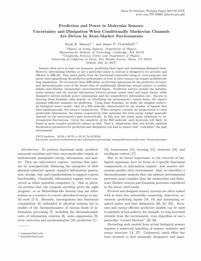
To illustrate the insights that arise from this, we study

an “optimal” Hill molecule model of ligand-gated chan-

nels; see Fig. 1. A Hill molecule is a conditionally Marko-

vian channel with its ligand concentration as input. We

assume that the ligand concentration is a realization of

a semi-Markov process, a generalization over previous ef-

forts that assumed Markovian [12] or Gaussian [27] pro-

cesses. Our generalization to arbitrarily temporally cor-

related inputs is necessary when, for instance, the Hill

molecule represents a nicotinic acetylcholine receptor on

a synapse and ligands are acetylcholine molecules since,

as a practical matter, neuronal dynamics are often non-

Markovian and non-Gaussian [31]. As a result, we find

that (i) increases in cooperativity (memory) of the Hill

molecule lead to increases in both predictive power and

power consumption, (ii) a large fraction of power con-

sumption comes from inefficient prediction, and (iii) sim-

ple gradient-based adaptation rules lead to hysteresis.

Background Central to our analysis is an apprecia-

tion of causal states (minimal sufficient statistics of pre-

diction and/or retrodiction), unifilar hidden semi-Markov

processes, and conditionally Markovian channels. We re-

view these concepts here, simultaneously introducing rel-

evant notation.

Environment Input symbols x take on any

value in the observation alphabet A. We

code the past of the input time series as←−x = . . . (x−2, τ−2), (x−1, τ−1), (x0, τ+) and the in-

Ligand Concentration

Time

xh

x

Hill Molecule

K x 0n

K c

FIG. 1. Hill molecule: (Top) Ion channel in a neuronal mem-brane in the open (left) and closed (right) states in whichions can and cannot travel through. (Below) Ligand concen-trations during the open-closed cycle of the molecule.

put’s future as −→x = (x0, τ−), (x1, τ1), (x2, τ2), . . ., where

τi is the total dwell time for symbol xi. To ensure a

unique coding, we stipulate that xi 6= xi+1. Note that

symbol x0 is seen for a total dwell time of τ+ + τ− = τ0;

that is, the present splits the dwell time τ0 into two.

As is typical,←−X is the random variable corresponding

to semi-infinite input pasts and−→X the random variable

corresponding to semi-infinite input futures. We now

briefly review the definition of causal states, as described

in Ref. [32]. Forward-time causal states S+, the minimal

sufficient statistics for prediction, are defined via the fol-

lowing equivalence relation: two semi-infinite pasts, ←−xand ←−x ′, are considered “predictively” equivalent if:

←−x ∼ε+ ←−x ′ ⇔ Pr(−→X |←−X =←−x ) = Pr(

−→X |←−X =←−x ′) .

The relation partitions the set of semi-infinite pasts into

clusters of pasts. Each cluster is a forward-time causal

state σ+. Reverse-time causal states S−, the minimal

sufficient statistics for retrodiction, are defined similarly.

Two semi-infinite futures, −→x and −→x ′, are considered

“retrodictively” equivalent if:

−→x ∼ε− −→x ′ ⇔ Pr(←−X |−→X = −→x ) = Pr(

←−X |−→X = −→x ′) .

This equivalence relation partitions the set of semi-

infinite futures into clusters, each cluster being a reverse-

time causal state σ−.

Forward- and reverse-time causal states are useful in

the ensuing calculations due to the following Markov

chains. First, forward-time causal states are a deter-

ministic function of the input past (σ+ = ε+(←−x )), and

reverse-time causal states are a deterministic function of

the input future (σ− = ε−(−→x )). Hence, we have the

Markov chains S+ → ←−X → −→

X and S− → −→X → ←−

X .

3

However, causal states are minimal sufficient statistics

of the past relative to the future and vice versa. And

so,←−X → S+ → −→X and

−→X → S− → ←−X are also valid

Markov chains. Invoking these Markov chains is called

causal shielding.

Let’s first address the more general case of unifilar hid-

den semi-Markov input, as in Ref. [30]. Forward-time

hidden states are labeled g, and causal states are thus

labeled by (g, x+, τ+). That is, the forward-time hid-

den state g, current emitted symbol x+, and time since

last symbol τ+ together comprise the forward-time causal

states for unifilar hidden semi-Markov input processes.

Dwell times are drawn from φg(τ); emitted symbols are

chosen with probability p(x|g); and g = ε+(g′, x′) is the

next hidden state given that the current hidden state is

g′ and the current emitted symbol is x′.

For the Hill molecule, we focus on semi-Markov in-

put. This greatly constrains the forward- and reverse-

time causal states, so that g and x+ are equivalent. The

forward-time causal states are thus described by the pair

(x+, τ+), where x+ is the input symbol infinitesimally

prior to the present and τ+ is the time since last symbol

(i.e., x−1). The reverse-time causal states are similarly

described by the pair (x−, τ−), where x− is the input

symbol infinitesimally after the present and τ− is the

time to next symbol (i.e., x1). Let T± be the random

variable describing time since (to) last (next) symbol.

The dwell time of symbol x has probability density func-

tion φx(τ), and the probability of observing symbol x

after x′ is q(x|x′). By virtue of how we have chosen to

encode our input: q(x|x) = 0.

Finally, the development to come requires our finding

the joint distribution ρ(σ+, σ−) of forward- and reverse-

time causal states. When the input is unifilar hidden

semi-Markov, efficiently finding ρ(σ+, σ−) is an open

problem. Nonetheless, we can say:

ρ(σ−|σ+) = ρ(g−, x−, τ−|g+, x+, τ+)

= δx+,x−

φg+(τ+ + τ−)

Φg+(τ+)p(g+|g−, x−) .

For semi-Markov input, this simplifies: ρ(σ+, σ−) =

ρ((x+, τ+), (x−, τ−)). As described in Ref. [30], we have:

ρ(x+, τ+) = µx+Φx+(τ+)p(x+) (1)

where:

Φx+(τ+) =

∫ ∞

τ+

φx+(t)dt, µx+ = 1/

∫ ∞

0

tφx+(t)dt ,

and p(x+) is the probability of observing symbol x+.

The latter probability is given by:

p(x+) = (diag(1/µx) eig1(q))x+.

The conditional distribution of reverse-time causal states

given forward-time causal states is then:

ρ(σ−|σ+) = ρ((x−, τ−)|(x+, τ+))

=φx+(τ+ + τ−)

Φx+(τ+)δx+,x− . (2)

Together, Eqs. (1) and (2) give the joint distribution

ρ(σ+, σ−) = ρ(σ+)ρ(σ−|σ+).

Sensory channel We assume the channel is condition-

ally Markovian. As such, its dynamics are fully specified

by input state-dependent kinetic rates. More precisely,

the channel state y, with corresponding random variable

Y , can take on any value in Y, and the rate at which

channel state y transfers to channel state y′ when the

input has value x is given by:

ky→y(x) := −∑

y′

ky→y′(x) .

Then, the probability p(y, t) of being in channel state y

at time t evolves as:

dp(y, t)

dt=∑

y′

ky′→y(x(t))p(y′, t) ,

where x(t) is the input symbol at time t.

To simplify notation and ease computation, we write

dynamical evolution rules in matrix-vector form. Let

~p(y, t) be the vector of probabilities that the channel is in

a particular state y at time t, and let M(x) be a matrix

of rates: My′,y(x) = ky→y′(x). Then, we have:

d~p(y, t)

dt= M(x(t))~p(y, t) . (3)

With this, it is clear that ~p(y, t) can oscillate or decay to a

steady state. The Perron-Frobenius theorem guarantees

that:

peq(x) := eig0(M(x)) ,

the probability distribution over channel states when lig-

and concentration is set to x, is unique.

Sensor Accuracy and Thermodynamics We

now introduce and justify predictive and dissipative met-

rics, present closed-form expressions for these metrics in

terms of aforementioned generators and channels, and ex-

plore the relationship between cooperativity in biochem-

ical sensing and prediction and dissipation.

4

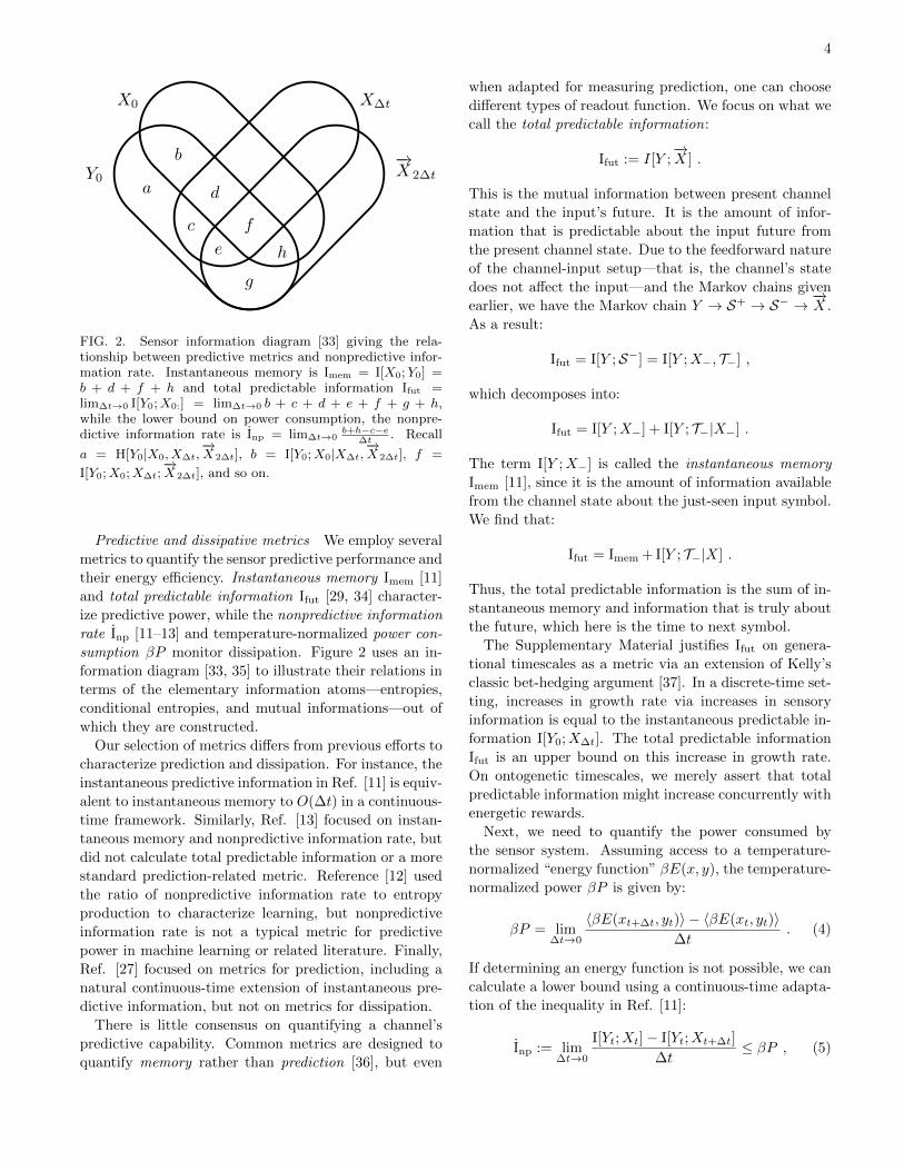
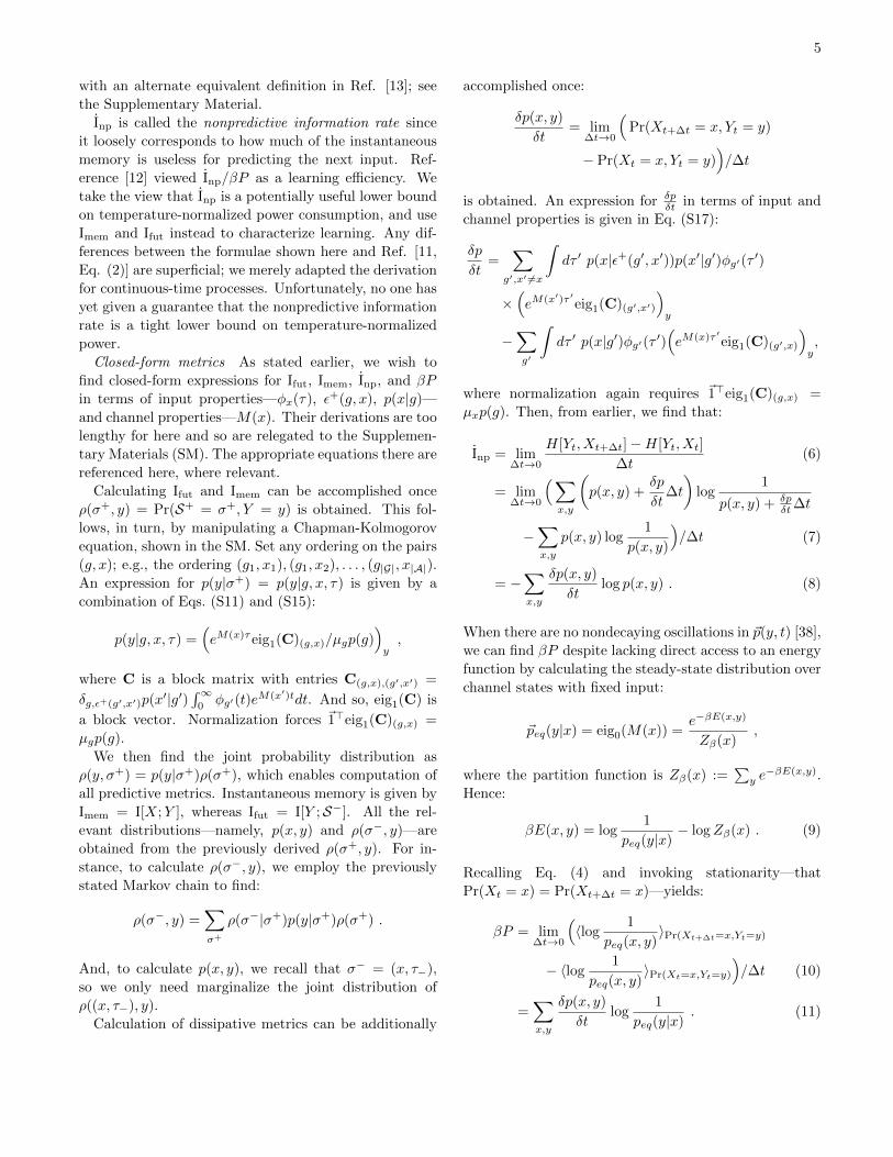
Y0

X0 X∆t

−→X 2∆t

a

b

c

g

d

he

f

FIG. 2. Sensor information diagram [33] giving the rela-tionship between predictive metrics and nonpredictive infor-mation rate. Instantaneous memory is Imem = I[X0;Y0] =b + d + f + h and total predictable information Ifut =lim∆t→0 I[Y0;X0:] = lim∆t→0 b + c + d + e + f + g + h,while the lower bound on power consumption, the nonpre-dictive information rate is Inp = lim∆t→0

b+h−c−e∆t

. Recall

a = H[Y0|X0, X∆t,−→X 2∆t], b = I[Y0;X0|X∆t,

−→X 2∆t], f =

I[Y0;X0;X∆t;−→X 2∆t], and so on.

Predictive and dissipative metrics We employ several

metrics to quantify the sensor predictive performance and

their energy efficiency. Instantaneous memory Imem [11]

and total predictable information Ifut [29, 34] character-

ize predictive power, while the nonpredictive information

rate Inp [11–13] and temperature-normalized power con-

sumption βP monitor dissipation. Figure 2 uses an in-

formation diagram [33, 35] to illustrate their relations in

terms of the elementary information atoms—entropies,

conditional entropies, and mutual informations—out of

which they are constructed.

Our selection of metrics differs from previous efforts to

characterize prediction and dissipation. For instance, the

instantaneous predictive information in Ref. [11] is equiv-

alent to instantaneous memory to O(∆t) in a continuous-

time framework. Similarly, Ref. [13] focused on instan-

taneous memory and nonpredictive information rate, but

did not calculate total predictable information or a more

standard prediction-related metric. Reference [12] used

the ratio of nonpredictive information rate to entropy

production to characterize learning, but nonpredictive

information rate is not a typical metric for predictive

power in machine learning or related literature. Finally,

Ref. [27] focused on metrics for prediction, including a

natural continuous-time extension of instantaneous pre-

dictive information, but not on metrics for dissipation.

There is little consensus on quantifying a channel’s

predictive capability. Common metrics are designed to

quantify memory rather than prediction [36], but even

when adapted for measuring prediction, one can choose

different types of readout function. We focus on what we

call the total predictable information:

Ifut := I[Y ;−→X ] .

This is the mutual information between present channel

state and the input’s future. It is the amount of infor-

mation that is predictable about the input future from

the present channel state. Due to the feedforward nature

of the channel-input setup—that is, the channel’s state

does not affect the input—and the Markov chains given

earlier, we have the Markov chain Y → S+ → S− → −→X .

As a result:

Ifut = I[Y ;S−] = I[Y ;X−, T−] ,

which decomposes into:

Ifut = I[Y ;X−] + I[Y ; T−|X−] .

The term I[Y ;X−] is called the instantaneous memory

Imem [11], since it is the amount of information available

from the channel state about the just-seen input symbol.

We find that:

Ifut = Imem + I[Y ; T−|X] .

Thus, the total predictable information is the sum of in-

stantaneous memory and information that is truly about

the future, which here is the time to next symbol.

The Supplementary Material justifies Ifut on genera-

tional timescales as a metric via an extension of Kelly’s

classic bet-hedging argument [37]. In a discrete-time set-

ting, increases in growth rate via increases in sensory

information is equal to the instantaneous predictable in-

formation I[Y0;X∆t]. The total predictable information

Ifut is an upper bound on this increase in growth rate.

On ontogenetic timescales, we merely assert that total

predictable information might increase concurrently with

energetic rewards.

Next, we need to quantify the power consumed by

the sensor system. Assuming access to a temperature-

normalized “energy function” βE(x, y), the temperature-

normalized power βP is given by:

βP = lim∆t→0

〈βE(xt+∆t, yt)〉 − 〈βE(xt, yt)〉∆t

. (4)

If determining an energy function is not possible, we can

calculate a lower bound using a continuous-time adapta-

tion of the inequality in Ref. [11]:

Inp := lim∆t→0

I[Yt;Xt]− I[Yt;Xt+∆t]

∆t≤ βP , (5)

5

with an alternate equivalent definition in Ref. [13]; see

the Supplementary Material.

Inp is called the nonpredictive information rate since

it loosely corresponds to how much of the instantaneous

memory is useless for predicting the next input. Ref-

erence [12] viewed Inp/βP as a learning efficiency. We

take the view that Inp is a potentially useful lower bound

on temperature-normalized power consumption, and use

Imem and Ifut instead to characterize learning. Any dif-

ferences between the formulae shown here and Ref. [11,

Eq. (2)] are superficial; we merely adapted the derivation

for continuous-time processes. Unfortunately, no one has

yet given a guarantee that the nonpredictive information

rate is a tight lower bound on temperature-normalized

power.

Closed-form metrics As stated earlier, we wish to

find closed-form expressions for Ifut, Imem, Inp, and βP

in terms of input properties—φx(τ), ε+(g, x), p(x|g)—

and channel properties—M(x). Their derivations are too

lengthy for here and so are relegated to the Supplemen-

tary Materials (SM). The appropriate equations there are

referenced here, where relevant.

Calculating Ifut and Imem can be accomplished once

ρ(σ+, y) = Pr(S+ = σ+, Y = y) is obtained. This fol-

lows, in turn, by manipulating a Chapman-Kolmogorov

equation, shown in the SM. Set any ordering on the pairs

(g, x); e.g., the ordering (g1, x1), (g1, x2), . . . , (g|G|, x|A|).

An expression for p(y|σ+) = p(y|g, x, τ) is given by a

combination of Eqs. (S11) and (S15):

p(y|g, x, τ) =(eM(x)τeig1(C)(g,x)/µgp(g)

)y,

where C is a block matrix with entries C(g,x),(g′,x′) =

δg,ε+(g′,x′)p(x′|g′)

∫∞0φg′(t)e

M(x′)tdt. And so, eig1(C) is

a block vector. Normalization forces ~1>eig1(C)(g,x) =

µgp(g).

We then find the joint probability distribution as

ρ(y, σ+) = p(y|σ+)ρ(σ+), which enables computation of

all predictive metrics. Instantaneous memory is given by

Imem = I[X;Y ], whereas Ifut = I[Y ;S−]. All the rel-

evant distributions—namely, p(x, y) and ρ(σ−, y)—are

obtained from the previously derived ρ(σ+, y). For in-

stance, to calculate ρ(σ−, y), we employ the previously

stated Markov chain to find:

ρ(σ−, y) =∑

σ+

ρ(σ−|σ+)p(y|σ+)ρ(σ+) .

And, to calculate p(x, y), we recall that σ− = (x, τ−),

so we only need marginalize the joint distribution of

ρ((x, τ−), y).

Calculation of dissipative metrics can be additionally

accomplished once:

δp(x, y)

δt= lim

∆t→0

(Pr(Xt+∆t = x, Yt = y)

− Pr(Xt = x, Yt = y))/∆t

is obtained. An expression for δpδt in terms of input and

channel properties is given in Eq. (S17):

δp

δt=

∑

g′,x′ 6=x

∫dτ ′ p(x|ε+(g′, x′))p(x′|g′)φg′(τ ′)

×(eM(x′)τ ′eig1(C)(g′,x′)

)y

−∑

g′

∫dτ ′ p(x|g′)φg′(τ ′)

(eM(x)τ ′eig1(C)(g′,x)

)y,

where normalization again requires ~1>eig1(C)(g,x) =

µxp(g). Then, from earlier, we find that:

Inp = lim∆t→0

H[Yt, Xt+∆t]−H[Yt, Xt]

∆t(6)

= lim∆t→0

(∑

x,y

(p(x, y) +

δp

δt∆t

)log

1

p(x, y) + δpδt∆t

−∑

x,y

p(x, y) log1

p(x, y)

)/∆t (7)

= −∑

x,y

δp(x, y)

δtlog p(x, y) . (8)

When there are no nondecaying oscillations in ~p(y, t) [38],

we can find βP despite lacking direct access to an energy

function by calculating the steady-state distribution over

channel states with fixed input:

~peq(y|x) = eig0(M(x)) =e−βE(x,y)

Zβ(x),

where the partition function is Zβ(x) :=∑y e−βE(x,y).

Hence:

βE(x, y) = log1

peq(y|x)− logZβ(x) . (9)

Recalling Eq. (4) and invoking stationarity—that

Pr(Xt = x) = Pr(Xt+∆t = x)—yields:

βP = lim∆t→0

(〈log

1

peq(x, y)〉Pr(Xt+∆t=x,Yt=y)

− 〈log1

peq(x, y)〉Pr(Xt=x,Yt=y)

)/∆t (10)

=∑

x,y

δp(x, y)

δtlog

1

peq(y|x). (11)

6

The distributions Pr(Xt+∆t = x, Yt = y) and Pr(Xt =

x, Yt = y) can be obtained from M(x). In other words,

when there are no recurrent cycles, we can calculate βP

directly from the kinetic rates ky→y′(x) and input gener-

ator (φg(τ), ε+(g, x), p(x|g)) alone.

Effect of cooperativity on prediction and dissipation

The Hill molecule is a common fixture in theoretical bi-

ology, as it is the simplest mechanistic model of coop-

erativity [39]. Recall Fig. 1. A Hill molecule can be in

one of two states, open or closed. When open, n ligand

molecules are bound; when closed, no ligand molecules

are bound. Hence, the state of the Hill molecule carries

information about the number of bound ligand molecules.

In other words, such molecules are sensors of their envi-

ronment.

Let us outline a simple dynamical model of the Hill

molecule. The rate of transition from closed C to open

O given a ligand concentration x is:

kC→O = kOxn . (12)

While the transition rate from open O to closed C is:

kO→C = kC . (13)

The steady-state distribution given fixed ligand concen-

tration is the familiar:

Preq(Y = O|X = x) =kOx

n

kC + kOxn

=xn

(kC/kO) + xn.

Although the mechanistic model makes sense only when

n is a nonnegative integer, this model is often used when

n is any nonnegative real number; increases in n can

still be thought of as increases in cooperativity. Equa-

tions (12)-(13) constitute a complete characterization of

channel properties.

Increasing the cooperativity n increases the steepness

of the molecule’s “binding curve”—the probability of be-

ing “on” as a function of concentration. In other words,

the sensor becomes more switch-like and less a propor-

tionately responding transducer of the input. If the con-

centration is greater than (kC/kO)1/n

, the switch is es-

sentially “on” if n is high. A more switch-like sensor

is useful if the optimal phenotype depends only upon

the condition “ligand concentration greater than X”.

Whereas, a less switch-like, smoother responding sensor

helps if the optimal phenotype depends on ligand con-

centration in a more graded manner.

The concentration scale is set by (kC/kO)1/n

, while

the time scale is set by 1/kC ; as such, we set both to

kO = kC = 1 without loss of generality. We imagine

0 2 4 6 8 10

n

0.00

0.01

0.02

0.03

0.04

0.05

0.06

0.07

0.08

0.09

Imem

Ifut

0 2 4 6 8 10

n

0

1

2

3

4

5

Inp

βP

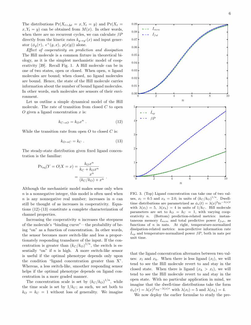
FIG. 3. (Top) Ligand concentration can take one of two val-

ues, xl = 0.5 and xh = 2.0, in units of (kC/kO)1/n. Dwell-

time distributions are parametrized as φx(t) = λ(x)2te−λ(x)t

with λ(xl) = 5, λ(xh) = 4 in units of 1/kC . Hill moleculeparameters are set to kO = kC = 1, with varying coop-erativity n. (Bottom) prediction-related metrics: instan-taneous memory Imem and total predictive power Ifut, asfunctions of n in nats. At right, temperature-normalizeddissipation-related metrics: non-predictive information rateInp and temperature-normalized power βP , both in nats perunit time.

that the ligand concentration alternates between two val-

ues: xl and xh. When there is less ligand (xl), we will

tend to see the Hill molecule revert to and stay in the

closed state. When there is ligand (xh > xl), we will

tend to see the Hill molecule revert to and stay in the

open state. With no particular application in mind, we

imagine that the dwell-time distributions take the form

φx(τ) = λ(x)2τe−λ(x)τ with λ(xl) = 5 and λ(xh) = 4.

We now deploy the earlier formulae to study the pre-

7

dictive capabilities and dissipative tendencies of a Hill

molecule subject to semi-Markov input. Previous stud-

ies of biological sensors found that increases in coopera-

tivity accompanied increases in channel capacity [40–42].

Others studied the thermodynamics of prediction of co-

operative biological sensors [12, 27], but did not use the

more general class of semi-Markov input and did not cal-

culate the full suite of metrics here, leaving much sensor

operation untouched.

An example—xl = 0.5, xh = 2.0 and kO = kC =

1.0, n = 2—illustrates that roughly 99% of Ifut is de-

voted to instantaneous memory Imem and roughly 25% of

βP is devoted to Inp. That is, the inefficiency in choosing

what information to store about the present input con-

tributes greatly to energetic inefficiency. These results

hold qualitatively even when the dwell-time distributions

are log-normal, i.e., are heavier-tailed.

Fig. 3 shows that increased cooperativity—that is,

increases in n—lead to increases in predictive perfor-

mance, qualitatively in line with Ref. [42]. Addition-

ally, the larger the cooperativity, the higher the fraction

of Imem / Ifut. Larger cooperativity, however, leads to

roughly linear increases in the power consumption and

the nonpredictive information rate, whereas increases

in predictive power take a more sigmoidal shape. We

therefore might prefer intermediate values of cooperativ-

ity (e.g., n ≈ 5) to larger values of cooperativity (e.g.,

n ≥ 10). This is qualitatively similar to the results of

Refs. [40, 41], in that physical constraints can force op-

timal information transmission at intermediate levels of

cooperativity.

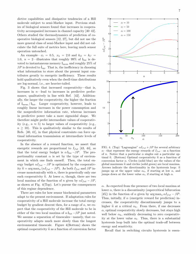
In the absence of a reward function, we assert that

energetic rewards are proportional to Ifut [43, 44], so

that the total energy budget is α Ifut−βP . The pro-

portionality constant α is set by the type of environ-

ment in which one finds oneself. Then, the total en-

ergy budget αIfut − βP is optimized by the cooperativ-

ity n = arg maxn (αIfut − βP ). As both Ifut and βP in-

crease monotonically with n, there is generically only one

such cooperativity n. At lower α, though, there are two

local maxima of the function of n given by αIfut − βP ,

as shown at Fig. 4(Top). Let’s pursue the consequences

of this regime dependence.

There are rules for how sensor biochemical parameters

adapt to the present environment. If adaptation rules for

cooperativity of a Hill molecule increase the total energy

budget by gradient descent then, for a range of α, we ex-

pect that the cooperativity of the Hill molecule to be in

either of the two local maxima of α Ifut−βP just noted.

We assume a separation of timescales—namely, that co-

operativity adapts much more slowly than the longest

environmental timescale. Figure 4(Bottom) shows the

optimal cooperativity n as a function of conversion factor

0 2 4 6 8 10

n

−4

−2

0

2

4

6

8

10

αI fut−βP

α = 10

α = 50

α = 100

α = 150

0 50 100 150 200

α

0

2

4

6

8

10

n

αhαl

FIG. 4. (Top) “Lagrangian” αIfut + βP for several arbitraryα—that represent the energy rewards of Ifut—as a functionof n. Notice that a particular α singles out a particular op-timal n. (Bottom) Optimal cooperativity n as a function ofconversion factor α. Circles (solid blue) are the values of theglobal maximum n and circles (solid green) are local maxima.Arrows indicate the directionality in the hysteresis loop: njumps up at the upper value αh, if starting at low α, andjumps down at the lower value αl, if starting at high α.

α. As expected from the presence of two local maxima at

lower α, there is a discontinuity (supercritical bifurcation

[45]) in the function of α given by arg maxn αIfut − βP .

Thus, initially, if α (energetic reward for prediction) in-

creases, the cooperativity discontinuously jumps to a

higher n at a critical αh. From there, if one decreases

α, optimal cooperativity slowly decreases, but stays high

well below αh, suddenly decreasing to zero cooperativ-

ity at the lower value αl. Thus, there is a substantial

hysteresis loop built into the optimal trade-off between

energy and sensitivity.

Recall that in switching circuits hysteresis is essen-

8

tial to adding stability to a switch’s response. Hystere-

sis stops “race” conditions in which the switch oscillates

wildly just as the threshold is passed, amplifying any

noise in the control and internal dynamics. In the Hill

molecule, hysteresis is helpful if a memory of past envi-

ronmental conditions (α) provides insight into future con-

ditions (future α). For example, the environment might

shift α suddenly to being low, but there is a replenish-

ment mechanism for the available energy that will soon

increase α again. Thus, we see that robustness to envi-

ronmental noise emerges naturally as the sensor adapts

to and anticipates changing external conditions.

Conclusion We provided closed-form expressions

for instantaneous memory, total predictable information,

nonpredictive information rate, and power consumption

for a conditionally Markovian channel subject to unifilar

hidden semi-Markov input.

In motivating these metrics for prediction and dissi-

pation on general timescales, we appealed to an exten-

sion of Kelly’s classic bet-hedging that arises from his

information-theoretic analysis of trading-off the benefits

of risky, but highly profitable resource investment against

the costs of sudden loss [37, 46]. Here, a sensor faces an

analogous challenge of high sensitivity but at an energy

cost that might be suddenly wasted when the environ-

mental conditions fluctuate. Similar bet-hedging strate-

gies have been implicated in other biological systems,

such as in seed germination in annual plants [47] and

bacteriophages [48] and in population biology [49, 50]

and evolution [46, 51] more generally. The present set-

ting, though, implicates such strategy optimization in a

substantially more elementary and primitive biological

subsystem.

Finally, we used these formulae to calculate the pre-

dictive performance and energetic inefficiency of a sim-

ple model of a biological sensor—a Hill molecule. We

found that increases in cooperativity yield increases in

both predictive performance and energy consumption

and that the relative balance between those increases nat-

urally leads to sensor robustness to environmental fluc-

tuations supported by dynamical hysteresis. Given the

Hill molecule’s simplicity as a model sensor, we expect

to find hysteresis and the resulting robustness in more

complex biological sensory systems.

The ease with which these various metrics were cal-

culated masks the difficulty of obtaining the necessary

closed-form expressions. (Cf. Supplementary Materials.)

We provided universal estimators for various predictive

and dissipative metrics for conditionally Markovian chan-

nels, as unifilar hidden semi-Markov processes are that

general. One practical consequence it that those wish-

ing to study the relationship between prediction and dis-

sipation need not simulate arbitrarily long trajectories.Instead, they can validate or invalidate predictive learn-

ing rules and sensor designs using the universal estima-

tors of these predictive and dissipative metrics. Then

they can efficiently search through parameter space for

“optimal” (predictive and energy-efficient) sensors. In

addition, given that the theories of random dynamical

systems and of input-dependent dynamical systems are

still under development [52], we believe the formulae pre-

sented here will lead in those domains to a precise gen-

eralization of time-scale matching for nonlinear systems

[27].

ACKNOWLEDGMENTS

We thank N. Ay, A. Bell, W. Bialek, S. Dedeo, C.

Hillar, I. Nemenman, and S. Still for useful conversa-

tions and the Santa Fe Institute for its hospitality during

visits, where JPC is an External Faculty member. This

material is based upon work supported by, or in part by,

the John Templeton Foundation grant 52095, the Foun-

dational Questions Institute grant FQXi-RFP-1609, the

U. S. Army Research Laboratory and the U. S. Army Re-

search Office under contract W911NF-13-1-0390. S.E.M.

was funded by an MIT Physics of Living Systems Fellow-

ship.

[1] C. H. Bennett. The thermodynamics of computation: a

review. Intl. J. Theo. Physics, 21(12):905–940, 1982.

[2] J. C. Maxwell. Theory of Heat. Longmans, Green and

Co., London, United Kingdom, ninth edition, 1888.

[3] L. Szilard. On the decrease of entropy in a thermody-

namic system by the intervention of intelligent beings.

Z. Phys., 53:840–856, 1929.

[4] D. Mandal and C. Jarzynski. Work and information pro-

cessing in a solvable model of Maxwell’s demon. Proc.

Natl. Acad. Sci. USA, 109(29):11641–11645, 2012.

[5] S. Deffner and C. Jarzynski. Information processing and

the second law of thermodynamics: An inclusive, hamil-

tonian approach. Phys. Rev. X, 3(4):041003, 2013.

[6] Here, when analyzing sensory information processing in

biological systems, we take care to distinguish intrin-

sic, functional, and useful computation [53–55]. Intrin-

sic computation refers to how a physical system stores

and transforms its historical information. We take func-

tional computation as information processing in a phys-

ical device that promotes the performance of a larger,

9

encompassing system. Whereas, we take useful computa-

tion as information processing in a physical device used

to achieve an external user’s goal. The first is well-suited

to analyzing structure in physical processes and deter-

mining if they are candidate substrates for any kind of

information processing. The second is well-suited for dis-

cussing biological sensors, while the third is well-suited

for discussing the benefits of contemporary digital com-

puters.

[7] J. M. R. Parrondo, J. M. Horowitz, and T. Sagawa. Ther-

modynamics of information. Nat. Physics, 11(2):131–139,

2015.

[8] C. Aghamohammdi and J. P. Crutchfield. Thermody-

namics of random number generation. Phys. Rev. E,

95(6):062139, 2017.

[9] M. Hinczewski and D. Thirumalai. Cellular signaling net-

works function as generalized Wiener-Kolmogorov filters

to suppress noise. Phys. Rev. X, 4(4):041017, 2014.

[10] A. B. Boyd, D. Mandal, and J. P. Crutch-

field. Correlation-powered information engines and

the thermodynamics of self-correction. Phys. Rev. E,

95(1):012152, 2017.

[11] S. Still, D. A. Sivak, A. J. Bell, and G. E. Crooks. Ther-

modynamics of prediction. Phys. Rev. Lett., 109:120604,

Sep 2012.

[12] A. C. Barato, D. Hartich, and U. Seifert. Efficiency

of cellular information processing. New J. Physics,

16(10):103024, 2014.

[13] J. M. Horowitz and M. Esposito. Thermodynamics with

continuous information flow. Phys. Rev. X, 4:031015, Jul

2014.

[14] A. B. Boyd, D. Mandal, and J. P. Crutchfield. Leverag-

ing environmental correlations: The thermodynamics of

requisite variety. J. Stat. Phys., 167(6):1555–1585, 2016.

[15] S. Goldt and U. Seifert. Stochastic thermodynamics of

learning. Phys. Rev. Lett., 118(1):010601, 2017.

[16] A. B. Boyd, D. Mandal, P. M. Riechers, and J. P.

Crutchfield. Transient dissipation and structural costs

of physical information transduction. Phys. Rev. Lett.,

118:220602, 2017.

[17] A. B. Boyd and J. P. Crutchfield. Maxwell demon dy-

namics: Deterministic chaos, the Szilard map, and the

intelligence of thermodynamic systems. Phys. Rev. Lett.,

116:190601, 2016.

[18] R. P. N. Rao and D. H. Ballard. Predictive coding in the

visual cortex: a functional interpretation of some extra-

classical receptive-field effects. Nat. Neurosci., 2(1):79–

87, 1999.

[19] S. E. Palmer, O. Marre, M. J. Berry, and W. Bialek.

Predictive information in a sensory population. Proc.

Natl. Acad. Sci. USA, 112(22):6908–6913, 2015.

[20] D. B. Chklovskii and A. A. Koulakov. Maps in the brain:

what can we learn from them? Annu. Rev. Neurosci.,

27:369–392, 2004.

[21] A. Hasenstaub, S. Otte, E. Callaway, and T. J. Sejnowski.

Metabolic cost as a unifying principle governing neuronal

biophysics. Proc. Natl. Acad. Sci. USA, 107(27):12329–

12334, 2010.

[22] We only consider online or real-time computations, so

that the oft-considered energy-speed-accuracy tradeoff

[56, 57] reduces to an energy-accuracy tradeoff.

[23] R. S. Sutton and A. G. Barto. Reinforcement learning:

An introduction. MIT Press, Cambridge, Massachusetts,

1998.

[24] M. L. Littman, R. S. Sutton, and S. P. Singh. In NIPS,

volume 14, pages 1555–1561, 2001.

[25] N. Brodu. Adv. Complex Sys., 14(05):761–794, 2011.

[26] D. Y. Little and F. T. Sommer. Learning and exploration

in action-perception loops. Closing the Loop Around Neu-

ral Systems, page 295, 2014.

[27] N. B. Becker, A. Mugler, and P. R. ten Wolde. Optimal

prediction by cellular signaling networks. Phys. Rev. lett.,

115(25):258103, 2015.

[28] F. Creutzig and H. Sprekeler. Predictive coding and the

slowness principle: An information-theoretic approach.

Neural Comp., 20(4):1026–1041, 2008.

[29] F. Creutzig, A. Globerson, and N. Tishby. Past-future

information bottleneck in dynamical systems. Phys. Rev.

E, 79(4):041925, 2009.

[30] S. Marzen and J. P. Crutchfield. Structure and random-

ness of continuous-time discrete-event processes. 2016.

arxiv.org:1704.04707.

[31] E. M. Izhikevich. Dynamical systems in neuroscience.

MIT press, Cambridge, Massachusetts, 2007.

[32] C. R. Shalizi and J. P. Crutchfield. Computational me-

chanics: Pattern and prediction, structure and simplicity.

J. Stat. Phys., 104:817–879, 2001.

[33] R. G. James, C. J. Ellison, and J. P. Crutchfield.

Anatomy of a bit: Information in a time series obser-

vation. CHAOS, 21(3):037109, 2011.

[34] S. Still, J. P. Crutchfield, and C. J. Ellison. Optimal

causal inference: Estimating stored information and ap-

proximating causal architecture. CHAOS, 20(3):037111,

2010.

[35] R. W. Yeung. A New Outlook on Shannon’s Information

Measures. IEEE Trans. Info. Th., 37(3):466–474, 1991.

[36] O. L. White, D. D. Lee, and H. Sompolinsky. Short-term

memory in orthogonal neural networks. Phys. Rev. Lett.,

92(14):148102, 2004.

[37] T. M. Cover and J. A. Thomas. Elements of Information

Theory. Wiley-Interscience, New York, second edition,

2006.

[38] J Schnakenberg. Network theory of microscopic and

macroscopic behavior of master equation systems. Rev.

Mod. Physics, 48(4):571, 1976.

[39] S. Marzen, H. G. Garcia, and R. Phillips. Statistical

mechanics of monod–wyman–changeux (mwc) models. J.

Mole. Bio., 425(9):1433–1460, 2013.

[40] G. Tkacik, A. M. Walczak, and W. Bialek. Optimizing

information flow in small genetic networks. Phys. Rev.

E, 80(3):031920, 2009.

[41] A. M. Walczak, G. Tkacik, and W. Bialek. Optimizing in-

formation flow in small genetic networks. II. Feed-forward

interactions. Phys. Rev. E, 81(4):041905, 2010.

[42] B. M. C. Martins and P. S. Swain. Trade-offs and

constraints in allosteric sensing. PLoS Comput. Bio.,

10

7(11):e1002261, 2011.

[43] S. Still. Information-theoretic approach to interactive

learning. EuroPhys. Lett., 85:28005, 2009. arxiv.org

physics 0709.1948.

[44] Naftali Tishby and Daniel Polani. Information theory of

decisions and actions. In Perception-action cycle, pages

601–636. Springer, 2011.

[45] S. H. Strogatz. Nonlinear Dynamics and Chaos: with ap-

plications to physics, biology, chemistry, and engineering.

Addison-Wesley, Reading, Massachusetts, 1994.

[46] C. T. Bergstrom and M. Lachmann. Shannon informa-

tion and biological fitness. In Information Theory Work-

shop, 2004. IEEE, volume IEEE 0-7803-8720-1, pages

50–54. IEEE, 2004.

[47] M. G. Bulmer. Delayed germination of seeds: Cohen’s

model revisited. Theo. Pop. Bio., 26:367–377, 1984.

[48] S. Maslov and K. Sneppen. Well-temperate phage: op-

timal bet-hedging against local environmental collapses.

Sci. Reports, 5:10523, 2015.

[49] D. Cohen. Optimizing reproduction in a randomly vary-

ing environment. J. Theo. Bio., 12:119–129, 1966.

[50] J. A. J. Metz, R. M. Nisbet, and S. A. H. Geritz. How

should we define fitness for general ecological scenarios?

Trends Ecol. Evol., 7:198–202, 1992.

[51] J. Seger and H. J. Brockmann. What is bet-hedging?

Oxford Surveys in Evolutionary Biology, 4:182–211, 1987.

[52] L. Arnold. Random dynamical systems. Springer Science

& Business Media, New York, New York, 2013.

[53] J. P. Crutchfield and K. Young. Inferring statistical com-

plexity. Phys. Rev. Let., 63:105–108, 1989.

[54] J. P. Crutchfield. The calculi of emergence: Compu-

tation, dynamics, and induction. Physica D, 75:11–54,

1994.

[55] J. P. Crutchfield and M. Mitchell. The evolution of

emergent computation. Proc. Natl. Acad. Sci., 92:10742–

10746, 1995.

[56] G. Lan, P. Sartori, S. Neumann, V. Sourjik, and Y. Tu.

The energy-speed-accuracy trade-off in sensory adapta-

tion. Nat. Physics, 8(5):422–428, 2012.

[57] S. Lahiri, J. Sohl-Dickstein, and S. Ganguli. A universal

tradeoff between power, precision and speed in physical

communication. arXiv:1603.07758, 2016.

1

Supplementary Materials

Prediction and Power in Molecular Sensors

Sarah E. Marzen and James P. Crutchfield

I. EXTENDING KELLY’S ARGUMENT

Although the use of mutual information for a biolog-

ical sensor may seem arbitrary, it gains operational sig-

nificance via a straightforward extension of Kelly’s bet-

hedging arguments [37, Ch. 6 of]. Here, we switch to a

discrete-time analysis. Kelly’s classic result states that a

population of organisms increases its expected log growth

rate by I[Yt;Xt+1]—the instantaneous predictive infor-

mation. Each organism stores information about the

past environments in a sensory variable y and chooses

stochastically from p(g|y) to exhibit phenotype g based

on this sensory variable. Kelly’s original derivation as-

sumed that only one phenotype can reproduce in each

possible environment. We extend this result by relaxing

this assumption, following Ref. [46]. Let nt be the num-

ber of organisms at time t; let p(g|yt) be the probability

that an organism expresses phenotype g given sensory

state yt; let xt be the sensory input at time t; and let

f(g, x) be the growth rate of phenotype g in environment

x. Then, we straightforwardly obtain:

nt+1 =∑

g

(p(g|yt)nt)f(g, xt+1)

=

(∑

g

p(g|yt)f(g, xt+1)

)nt .

This yields an expected log growth rate of:

r =

⟨log

nt+1

nt

⟩

=

⟨log

(∑

g

p(g|yt)f(g, xt+1)

)⟩

=∑

yt,xt+1

p(yt, xt+1) log

(∑

g

p(g|yt)f(g, xt+1)

).

We seek the bet-hedging strategy that maximizes ex-

pected log growth rate. That is, maximize r, subject

to the constraint that∑g p(g|yt) = 1 for all yt, via the

Lagrangian:

L =∑

yt,xt+1

p(yt, xt+1) log

(∑

g

p(g|yt)f(g, xt+1)

)

+∑

yt

λyt∑

g

p(g|yt) ,

with respect to p(g|yt). Following Ref. [46], let x be the

vector of optimal p(g|yt), let p be the vector of p(x|yt),and let W be the matrix with elements f(g, x). Then,

we find that:

(Wx)k = pk/∑

j

(W−1)jk

→ x = W−1(p� [1>W−1]�−1

)

is the maximizing conditional distribution if it is in the

interior of the simplex. This gives an expected log growth

rate:

r∗ =∑

yt,xt+1

p(yt, xt+1) logp(xt+1|yt)∑g(W

−1)g,xt+1

= −H[Xt+1|Yt]−∑

xt+1

p(xt+1) log∑

g

((W−1)g,xt+1) .

The difference between this expected log growth rate and

the maximal expected log growth rate of a population

without any sensing capabilities is:

∆r∗ = −H[Xt+1|Yt] +H[Xt+1]

= I[Yt;Xt+1] . (S1)

This is exactly the instantaneous predictive information,

which lower bounds the total predictable information cal-

culated here.

II. REVISITING THE “THERMODYNAMICS

OF PREDICTION”

For completeness, we review the derivation of Eq. (5).

Let xt represent the input at time t, let yt represent the

sensor state at time t, and let E(x, y) denote the system’s

energy function. We assume constant temperature. The

system’s temperature-normalized nonequilibrium free en-

ergy Fneq is given by:

βFneq[p(x, y)] = β〈E(x, y)〉 −H[Y |X] . (S2)

The validity of Ref. [11]’s derivation rests on the nonequi-

librium free energy being a Lyapunov function. Intu-

itively, this corresponds to an assumption that the system

reduces its nonequilibrium free energy when the sensor

thermalizes. If so, then:

βFneq[p(xt+∆t, yt)] ≥ βFneq[p(xt+∆t, yt+∆t)] ,

2

giving:

0 ≤ βFneq[p(xt+∆t, yt)]− βFneq[p(xt+∆t, yt+∆t)]

≤ (β〈E(xt+∆t, yt)〉 −H[Yt|Xt+∆t])

− (β〈E(xt+∆t, yt+∆t)〉 −H[Yt+∆t|Xt+∆t])

and, from stationarity, 〈E(xt+∆t, yt+∆t)〉 = 〈E(xt, yt)〉and H[Yt+∆t|Xt+∆t] = H[Yt|Xt], giving:

0 ≤ β (〈E(xt+∆t, yt)〉 − 〈E(xt, yt)〉)− (H[Yt|Xt+∆t]−H[Yt|Xt])

≤ lim∆t→0

β (〈E(xt+∆t, yt)〉 − 〈E(xt, yt)〉)∆t

− lim∆t→0

H[Yt|Xt+∆t]−H[Yt|Xt]

∆t.

We recognize the first term as the temperature-

normalized power βP . Hence, the nonpredictive infor-

mation rate is the increase in unpredictability of sensor

state Yt given a slightly delayed environmental state:

Inp := lim∆t→0

H[Yt|Xt+∆t]−H[Yt|Xt]

∆t≤ βP . (S3)

From standard information theory identities [37]—

namely, I[U ;V ] = H[U ]−H[U |V ]—we see that:

H[Yt|Xt+∆t]−H[Yt|Xt] = I[Yt;Xt]− I[Yt;Xt+∆t] .

Reference [11]’s main result follows directly:

Inp = lim∆t→0

I[Yt;Xt]− I[Yt;Xt+∆t]

∆t≤ βP . (S4)

Differences in presentation come from the difference

between discrete- and continuous-time formulations. To

make this clear, we present a continuous-time formula-

tion of the same result, following Ref. [13]. We start

from βFneq[p(xt, yt′)] being a Lyapunov function in t′:

0 ≥ β ∂Fneq[p(xt, yt′)]∂t′

= β∂

∂t′〈E(xt, yt′)〉

∣∣∣t′=t− ∂

∂t′H[Yt′ |Xt]|t′=t

= β

⟨∂E(xt, yt)

∂ytyt

⟩− ∂

∂t′H[Yt′ |Xt]|t′=t .

We then recognize β⟨∂E(xt,yt)

∂ytyt

⟩as the temperature-

normalized rate of heat dissipation βQ, so that:

βQ ≤ ∂

∂t′H[Yt′ |Xt]|t′=t .

In nonequilibrium steady state, ddt 〈E〉 = 0 and

ddt H[Yt|Xt] = 0. As a result, βQ+ βP = 0 and:

∂

∂t′H[Yt′ |Xt]|t′=t = − ∂

∂t′H[Yt|Xt′ ]|t′=t ,

giving:

βP ≥ ∂

∂t′H[Yt|Xt′ ]|t′=t , (S5)

which we recognize as the continuous-time formulation of

Eq. (S3). Again invoking stationarity, ddt H[Xt] = 0, and

so:

βP ≥ − ∂

∂t′I[Xt′ ;Yt]|t′=t , (S6)

the continuous-time formulation of Eq. (S4). We have, in

Eqs. (S3), (S4), (S5), and (S6), four equivalent definitions

for the nonpredictive information rate in the nonequilib-

rium steady state limit.

III. CLOSED-FORM EXPRESSIONS FOR UNIFILAR HIDDEN SEMI-MARKOV ENVIRONMENTS

To find ρ(σ+, y), we start with the following:

Pr(S+t+∆t = (g, x, τ), Yt+∆t = y)

=∑

g′,x,′,τ ′,y′

Pr(S+t+∆t = (g, x, τ), Yt+∆t = y|S+

t = (g′, x′, τ ′), Yt = y′) Pr(S+t = (g′, x′, τ ′), Yt = y′) . (S7)

We decompose the transition probability using the feedforward nature of the transducer as:

Pr(S+t+∆t = (g, x, τ), Yt+∆t = y|S+

t = (g′, x′, τ ′), Yt = y′) = Pr(S+t+∆t = (g, x, τ)|S+

t = (g′, x′, τ ′))

× Pr(Yt+∆t = y|S+t = (g′, x′, τ ′), Yt = y′) .

3

From the setup, we have:

Pr(Yt+∆t = y|S+t = (g′, x′, τ ′), Yt = y′) =

{ky′→y(x′)∆t y 6= y′

1− ky′→y′(x′)∆t y = y′,

with corrections of O(∆t2).

Now split this into two cases. As long as τ > ∆t, so that x = x′, we have:

Pr(S+t+∆t = (g, x, τ)|S+

t = (g′, x′, τ ′)) =Φg(τ)

Φg(τ ′)δ(τ − (τ ′ + ∆t))δx,x′δg,g′ .

Then, Eq. (S7) reduces to

Pr(S+t+∆t = (g, x, τ), Yt+∆t = y) =

∑

y′

Pr(S+t+∆t = (g, x, τ)|S+

t = (g, x, τ −∆t)) Pr(Yt+∆t = y|S+t = (g, x, τ −∆t), Yt = y′)

× Pr(S+t = (g, x, τ −∆t), Yt = y′)

=∑

y′ 6=y

Pr(S+t+∆t = (g, x, τ)|S+

t = (g, x, τ −∆t)) Pr(Yt+∆t = y|S+t = (g, x, τ −∆t), Yt = y′)

× Pr(S+t = (g, x, τ −∆t), Yt = y′)

+ Pr(S+t+∆t = (g, x, τ)|S+

t = (g, x, τ −∆t)) Pr(Yt+∆t = y|S+t = (g, x, τ −∆t), Yt = y)

× Pr(S+t = (g, x, τ −∆t), Yt = y)

=∑

y′ 6=y

Φg(τ)

Φg(τ −∆t)ky′→y(x) Pr(S+

t = (g, x, τ −∆t), Yt = y′)∆t

+Φg(τ)

Φg(τ −∆t)(1− ky→y(x)∆t) Pr(S+

t = (g, x, τ −∆t), Yt = y) , (S8)

plus terms of O(∆t2). We Taylor expand Φg(τ + ∆t) = Φg(τ)− φg(τ)∆t to find:

Φg(τ)

Φg(τ −∆t)= 1− φg(τ)

Φg(τ)∆t‘,

plus terms of O(∆t2). And, similarly, assuming differentiability, we write:

Pr(S+t = (g, x, τ −∆t), Yt = y′) = Pr(S+

t = (g, x, τ), Yt = y′)− d

dτPr(S+

t = (g, x, τ), Yt = y′)∆t‘,

plus terms of O(∆t2). Substitution into Eq. (S8) then gives:

Pr(S+t+∆t = (g, x, τ), Yt+∆t = y) =

∑

y′ 6=y

ky′→y(x) Pr(S+t = (g, x, τ), Yt = y′)

∆t+ Pr(S+

t = (g, x, τ), Yt = y)

− dPr(S+t = (g, x, τ), Yt = y)

dτ∆t− φg(τ)

Φg(τ)Pr(S+

t = (g, x, τ), Yt = y)∆t

− ky→y(x) Pr(S+t = (g, x, τ), Yt = y)∆t ,

plus terms of O(∆t2). For notational ease, we denote:

ρ((g, x, τ), y) := Pr(S+t = (x, τ), Yt = y) ,

4

which is equal to Pr(S+t+∆t = (g, x, τ), Yt+∆t = y) since we assumed the system is in a NESS. Then we have:

ρ((g, x, τ), y) =

∑

y′ 6=y

ky′→y(x)ρ((g, x, τ), y′)

∆t+ ρ((g, x, τ), y)− dρ((g, x, τ), y)

dτ∆t

− φg(τ)

Φg(τ)ρ((g, x, τ), y)∆t− ky→y(x)ρ((g, x, τ), y)∆t

plus corrections of O(∆t2). We are left equating the coefficient of the O(∆t) term to 0:

dρ((g, x, τ), y)

dτ=∑

y′ 6=y

ky′→y(x)ρ((g, x, τ), y′)− φg(τ)

Φg(τ)ρ((g, x, τ), y)− ky→y(x)ρ((g, x, τ), y) . (S9)

Our task is simplified if we separate:

ρ((g, x, τ), y) = p(y|g, x, τ)ρ(g, x, τ)

and if we recall that;

ρ(g, x, τ) = µgΦg(τ)p(g)p(x|g) .

These give:

dρ(g, x, τ)

dτ= −µgφg(τ)p(x)p(x|g). (S10)

Plugging Eq. (S10) into Eq. (S9) yields:

dp(y|x, τ)

dτρ(g, x, τ)− µgφg(τ)p(g)p(x|g)p(y|g, x, τ)

=∑

y′ 6=y

ky′→y(x)ρ(g, x, τ)p(y′|g, x, τ)− φg(τ)

Φg(τ)ρ(g, x, τ)p(y|g, x, τ)− ky→y(x)ρ(g, x, τ)p(y|g, x, τ) ,

where we note that:

µgφg(τ)p(g)p(x|g)p(y|g, x, τ) =φg(τ)

Φg(τ)ρ(g, x, τ)p(y|g, x, τ) .

Hence, we are left with:

dp(y|g, x, τ)

dτ=∑

y′ 6=y

ky′→y(x)p(y′|g, x, τ)− ky→y(x)p(y|g, x, τ) .

We can summarize this ordinary differential equation in matrix-vector notation as follows. Let ~v(g, x, τ) be the

vector:

~v(g, x, τ) :=

p(y1|g, x, τ)

...

p(y|Y||g, x, τ)

.

We have:

d~v

dτ= M(x)~v .

5

The solution to the equation above is:

~v(g, x, τ) = eM(x)τ~v(g, x, 0) . (S11)

The structure of M(x) guarantees that probability is conserved, as long as 1>~v(g, x, 0) = 1 for all x ∈ A.

Our next task is to find expressions for ~v(g, x, 0). We do this by considering Eq. (S7) in the limit that τ < ∆t.

More straightforwardly, we consider the equation:

ρ((g, x, 0), y) =∑

g′,x′

∫ ∞

0

dτφg′(τ)

Φg′(τ)δg,ε+(g′,x′)p(x|g)ρ((g′, x′, τ), y) , (S12)

which is based on the following logic. For probability to flow into ρ((g, x, 0), y) from ρ((g′, x′, τ), y′), we need the dwell

time for symbol x′ to be exactly τ and for y′ = y. (The latter comes from the unlikelihood of switching both channel

state and input symbol at the same time.) Again decomposing:

ρ((g′, x′, τ), y) = p(y|g′, x′, τ)ρ(g′, x′, τ)

= µg′Φg′(τ)p(g′)p(x′|g′)p(y|g′, x′, τ) (S13)

and, thus, as a special case:

ρ((g, x, 0), y) = p(y|g, x, 0)p(g)p(x|g)µg . (S14)

Plugging both Eqs. (S13) and (S14) into Eq. (S12), we find:

µgp(g)p(x|g)p(y|g, x, 0) =∑

g′,x′

∫ ∞

0

µg′p(g′)p(x′|g′)φg′(τ)δg,ε+(g′,x′)p(x|g)p(y|g′, x′, τ)dτ

µgp(g)p(y|g, x, 0) =∑

g′,x′

∫ ∞

0

µg′p(g′)p(x′|g′)φg′(τ)δg,ε+(g′,x′)p(y|g′, x′, τ)dτ .

Using Eq. (S11), we see that p(y|g′, x′, τ) =(eM(x′)τ~v(g′, x′, 0)

)y

and p(y|g, x, 0) = (~v(g, x, 0))y. So, we have:

µgp(g)~v(g, x, 0) =∑

g′,x′

µg′δg,ε+(g′,x′)p(g′)p(x′|g′)

(∫ ∞

0

φg′(τ)eM(x′)τdτ

)~v(g′, x′, 0) .

If we form the composite vector ~V as:

~U =

~u(g1, x1)

~u(g1, x2)...

~u(g|G|, x|A|)

:=

µg1p(g1)~v(g1, x1, 0)

...

µg|G|p(g|G|)~v(g|G|, x|A|, 0)

and the matrix (written in block form) as:

C :=

C(g1,x1)→(g1,x1) C(g1,x2)→(g1,x1) . . .

C(g1,x1)→(g1,x2) C(g1,x2)→(g1,x2) . . ....

.... . .

,

6

with:

C(g′,x′)→(g,x) = δg,ε+(g′,x′)p(x′|g′)

∫ ∞

0

φg′(t)eM(x′)tdt ,

we then have:

~U = eig1(C) . (S15)

Finally, we must normalize ~u(x) appropriately. We do this by recalling that 1>~v(g, x, 0) = 1, since ~v(g, x, 0) is a vector

of probabilities. Then we have:

~u(g, x)→ ~u(g, x)

1>~u(g, x)µgp(g) .

for each g, x.

To calculate predictive metrics—i.e., Imem and Ifut—we need p(x, y) and p(y, σ−). The former is a marginalization

of p(σ+, y) that we just calculated. The second can be calculated via:

p(σ−, y) =∑

σ+

p(σ−|σ+)p(y, σ+) ,

where

p(σ−|σ+) = p((g−, x−, τ−)|(g+, x+, τ+))

= δx+,x−p(g−|g+, x+)µg+φg+

(τ+ + τ−) .

Hence, we turn our attention to dissipative metrics.

For calculation of dissipative metrics, we only need:

δp

δt= lim

∆t→0

Pr(Xt+∆t = x, Yt = y)− Pr(Xt = x, Yt = y)

∆t.

Moreover, we can use the Markov chain Yt → S+t → Xt+∆t to compute it:

Pr(Xt+∆t = x, Yt = y) =∑

σ+

Pr(Xt+∆t = x|S+t = σ+) Pr(Yt = y,S+

t = σ+) .

We have:

Pr(Xt+∆t = x|S+t = σ+) = Pr(Xt+∆t = x|S+

t = (g′, x′, τ ′))

=

Φg′ (τ′+∆t)

Φg′ (τ′) x = x′

φg′ (τ′)

Φg′ (τ′)p(x|ε+(g′, x′))∆t x 6= x′

.

7

This, combined with p(σ+, y), gives:

Pr(Xt+∆t = x, Yt = y) =∑

g′,x′ 6=x

∫dτ ′ ρ((g′, x′, τ ′), y)

φg′(τ′)

Φg′(τ ′)∆t p(x|ε+(g′, x′))

+∑

g′

∫dτ ′

Φg′(τ′ + ∆t)

Φg′(τ ′)ρ((g′, x′, τ ′), y)

= Pr(Xt = x, Yt = y) + ∆t( ∑

g′,x′ 6=x

∫dτ ′p(x|ε+(g′, x′))

φg′(τ′)

Φg′(τ ′)ρ((g′, x′, τ ′), y)

−∑

g′

∫dτ ′

φg′(τ′)

Φg′(τ ′)ρ((g′, x, τ ′), y)

),

correct to O(∆t). Recalling that:

ρ((g′, x′, τ ′), y) = ρ(g′, x′, τ ′)p(y|g′, x′, τ ′)= p(x′|g′)Φg′(τ ′)

(eM(x′)τ ′~u(g′, x′)

)y,

gives:

δp

δt= lim

∆t→0

Pr(Xt+∆t = x, Yt = y)− Pr(Xt = x, Yt = y)

∆t

=∑

g′,x′ 6=x

∫dτ ′p(x|ε+(g′, x′))

φg′(τ′)

Φg′(τ ′)ρ((g′, x′, τ ′), y)−

∑

g′

∫dτ ′

φg′(τ′)

Φg′(τ ′)ρ((g′, x, τ ′), y) (S16)

=∑

g′,x′ 6=x

∫dτ ′ p(x|ε+(g′, x′))p(x′|g′)φg′(τ ′)

(eM(x′)τ ′~u(g′, x′)

)y

−∑

g′

∫dτ ′ p(x|g′)φg′(τ ′)

(eM(x)τ ′~u(g′, x)

)y. (S17)

From this, Eqs. (8) and (11) can be used to calculate Inp and βP .

IV. SPECIALIZATION TO SEMI-MARKOV INPUT

Up to this point, we wrote expressions for the general case of unifilar hidden semi-Markov input. We now specialize

to the semi-Markov input case. A great simplification ensues: hidden states g are the current emitted symbols x.

Recall that, in an abuse of notation, q(x|x′) is now the probability of observing symbol x after seeing symbol x′.

Hence, forward-time causal states are given by the pair (x, τ). The analog of Eq. (S11) is:

~p(y|x, τ) = eM(x)τ~p(y|x, 0) ,

and we define vectors:

~u(x) := µxp(x)~p(y|x, 0) .

The large vector:

~U :=

~u(x1)

...

~u(x|A)

8

is the eigenvector eig1(C) of eigenvalue 1 of the matrix:

C =

0 q(x1|x2)∫∞

0φx2

(τ)eM(x2)τdτ

. . .

q(x2|x1)∫∞

0φx1

(τ)eM(x1)τdτ

. . ....

.... . .

‘,

where normalization requires 1>~u(x) = µxp(x).

We continue by finding p(y), since from this we obtain H[Y ]. We do this via straightforward marginalization:

p(y) =∑

σ+

ρ(σ+, y) =∑

σ+

p(y|σ+)ρ(σ+)

=∑

x

∫ ∞

0

p(y|x, τ)ρ(x, τ) dτ

=∑

x

∫ ∞

0

(eM(x)τ~v(x, 0)

)yµxp(x)Φx(τ)dτ

=∑

x

((∫ ∞

0

eM(x)τΦx(τ)dτ

)~u(x)

)

y

.

This implies that:

~p(y) =∑

x

(∫ ∞

0

eM(x)τΦx(τ)dτ

)~u(x) .

From earlier, recall that ~u(x) := µxp(x)~p(y|x, 0).

Next, we aim to find p(x, y), again via marginalization:

p(x, y) =

∫ ∞

0

ρ((x, τ), y)dτ

=

∫ ∞

0

µxp(x)Φx(τ)p(y|x, τ)dτ

=

∫ ∞

0

µxp(x)Φx(τ)(eM(x)τ~v(x, 0)

)ydτ

=

((∫ ∞

0

eM(x)τΦx(τ)dτ

)~u(x)

)

y

. (S18)

From the joint distribution p(x, y), we easily numerically obtain I[X;Y ], since |A| <∞ and |Y| <∞.

For notational ease, we introduced Tt in this section as the random variable for the time since last symbol, whose

realization is τ . Finally, we require p(y|σ−) to calculate H[Y |S−], which we can then combine with H[Y ] to get an

estimate for Ifut. We utilize the Markov chain Y → S+ → S−, as stated earlier, and so have:

p(y|σ−) =∑

σ+

ρ(y, σ+|σ−)

=∑

σ+

p(y|σ+, σ−)ρ(σ+|σ−)

=∑

σ+

p(y|σ+)ρ(σ+|σ−) .

9

Eq. (S11) gives us p(y|σ+) as:

p(y|σ+) = p(y|x+, τ+)

=(eM(x+)τ+~v(x+, 0)

)y

and Eq. (2) gives us ρ(σ+|σ−) after some manipulation:

ρ(σ+|σ−) = ρ((x+, τ+)|(x−, τ−))

= δx+,x−

φx−(τ+ + τ−)

Φx−(τ−).

Combining the two equations gives:

p(y|x−, τ−) =∑

x+

∫ ∞

0

δx+,x−

φx−(τ+ + τ−)

Φx−(τ−)

(eM(x+)τ+~v(x+, 0)

)ydτ+

=1

Φx−(τ−)

((∫ ∞

0

φx−(τ+ + τ−)eM(x−)τ+dτ+

)~v(x−, 0)

)

y

.

From this conditional distribution, we compute H[Y |S− = σ−], and so H[Y |S−] = 〈H[Y |S− = σ−]〉ρ(σ−). In more

detail, define:

Dx(τ) :=

∫ ∞

0

φx(τ + s)eM(x)sds ,

and we have:

~p(y|x−, τ−) = Dx−(τ−)~u(x−)/µx−p(x−)Φx−(τ−) .

This conditional distribution gives:

H[Y |X− = x−, T− = τ−] = −∑

y

p(y|x−, τ−) log p(y|x−, τ−)

= −1>(

Dx−(τ−)~u(x−)

µx−p(x−)Φx−(τ−)log

(Dx−(τ−)~u(x−)

µx−p(x−)Φx−(τ−)

))

= − 1

µx−p(x−)Φx−(τ−)

(1>((Dx−(τ−)~u(x−)) log(Dx−(τ−)~u(x−))

)

− 1>(Dx−(τ−)~u(x−)) log(µx−p(x−)Φx−(τ−))).

We recognize the factor µx−p(x−)Φx−(τ−) as ρ(x−, τ−) and so we find that:

H[Y |X−, T−] =∑

x−

∫ ∞

0

ρ(x−, τ−) H[Y |X− = x−, T− = τ−]dτ−

= −∫ ∞

0

∑

x−

1>((Dx−(τ−)~u(x−)) log(Dx−(τ−)~u(x−))

) dτ−

+

∫ ∞

0

∑

x−

1>Dx−(τ−)~u(x−) log(µx−p(x−)Φx−(τ−))

dτ− .

This, combined with earlier formula for H[Y ], gives Ifut.

Finally, we wish to find an expression for the nonpredictive information rate Inp. We review the somewhat compact

derivation of δpδt in the more general case, specialized for semi-Markov input. This requires finding an expression for

10

Pr(Yt = y,Xt+∆t = x) as an expansion in ∆t. We start as usual:

Pr(Yt = y,Xt+∆t = x) =∑

x′

∫ ∞

0

Pr(Yt = y,Xt+∆t = x,Xt = x′, Tt = τ)dτ

and utilize the Markov chain Yt → S+t → Xt+∆t, giving:

Pr(Yt = y,Xt+∆t = x) =∑

x′

∫ ∞

0

Pr(Yt = y|Xt = x′, Tt = τ) Pr(Xt+∆t = x|Xt = x′, Tt = τ)ρ(x′, τ)dτ . (S19)

We have Pr(Yt = y|Xt = x, Tt = τ) from Eq. (S11). So, we turn our attention to finding Pr(Xt+∆t = x|Xt = x′, Tt =

τ). Some thought reveals that:

Pr(Xt+∆t = x|Xt = x′, Tt = τ) =

{q(x|x′) φx′ (τ)

Φx′ (τ)∆t x 6= x′

Φx′ (τ+∆t)Φx′ (τ) x = x′

, (S20)

plus corrections of O(∆t2). We substitute Eq. (S20) into Eq. (S19) to get:

Pr(Yt = y,Xt+∆t = x) =

∑

x′ 6=x

∫ ∞

0

Pr(Yt = y|Xt = x′, Tt = τ)q(x|x′) φx′(τ)

Φx′(τ)ρ(x′, τ)dτ

∆t

+

∫ ∞

0

Pr(Yt = y|Xt = x, Tt = τ)Φx(τ + ∆t)

Φx(τ)ρ(x, τ)dτ ,

plus corrections of O(∆t2). Recalling:

Φx(τ + ∆t)

Φx(τ)= 1− φx(τ)

Φx(τ)∆t ,

plus corrections of O(∆t2), we simplify further:

Pr(Yt = y,Xt+∆t = x) =

∑

x′ 6=x

∫ ∞

0

Pr(Yt = y|Xt = x′, Tt = τ)q(x|x′) φx′(τ)

Φx′(τ)ρ(x′, τ)dτ

∆t

+

∫ ∞

0

Pr(Yt = y|Xt = x, Tt = τ)ρ(x, τ)dτ

−(∫ ∞

0

Pr(Yt = y|Xt = x, Tt = τ)φx(τ)

Φx(τ)ρ(x, τ)dτ

)∆t ,

plus O(∆t2) corrections. We notice that:

∫ ∞

0

Pr(Yt = y|Xt = x, Tt = τ)ρ(x, τ)dτ = Pr(Yt = y,Xt = x) ,

so that:

lim∆t→0

Pr(Yt = y,Xt+∆t = x)− Pr(Yt = y,Xt = x)

∆t=∑

x′ 6=x

∫ ∞

0

Pr(Yt = y|Xt = x′, Tt = τ)q(x|x′) φx′(τ)

Φx′(τ)ρ(x′, τ)dτ

−∫ ∞

0

Pr(Yt = y|Xt = x, Tt = τ)φx(τ)

Φx(τ)ρ(x, τ)dτ .

11

Substituting Eqs. (S11) and (1) into the above expressions yields:

∑

x′ 6=x

∫ ∞

0

Pr(Yt = y|Xt = x′, Tt = τ)q(x|x′) φx′(τ)

Φx′(τ)ρ(x′, τ)dτ =

∑

x′

q(x|x′)((∫ ∞

0

φx′(τ)eM(x′)τdτ

)~u(x′)

)

y

and:

∫ ∞

0

Pr(Yt = y|Xt = x, Tt = τ)φx(τ)

Φx(τ)ρ(x, τ)dτ =

((∫ ∞

0

φx(τ)eM(x)τdτ

)~u(x)

)

y

,

so that we have:

lim∆t→0

Pr(Yt = y,Xt+∆t = x)− Pr(Yt = y,Xt = x)

∆t

=(∑

x′

q(x|x′)(∫ ∞

0

φx′(τ)eM(x′)τdτ

)~u(x′)−

(∫ ∞

0

φx(τ)eM(x)τdτ

)~u(x)

)y.

For notational ease, denote the lefthand side as δp(x, y)/δt. The nonpredictive information rate is given by:

Inp = lim∆t→0

I[Xt;Yt]− I[Xt+∆t;Yt]

∆t

= lim∆t→0

(H[Xt] +H[Yt]−H[Xt, Yt])− (H[Xt+∆t] + H[Yt]−H[Xt+∆t, Yt])

∆t

= lim∆t→0

H[Xt+∆t, Yt]−H[Xt, Yt]

∆t,

where we utilize stationarity to assert H[Xt] = H[Xt+∆t]. Then, correct to O(∆t), we have:

H[Xt+∆t, Yt] = −∑

x,y

(p(x, y) +

δp(x, y)

δt∆t

)log

(p(x, y) +

δp(x, y)

δt∆t

)

= −∑

x,y

p(x, y) log p(x, y)−∑

x,y

p(x, y)δp(x, y)/δt

p(x, y)∆t−

∑

x,y

δp(x, y)

δtlog p(x, y)∆t

= H[Xt;Yt]−∑

x,y

δp(x, y)

δtlog p(x, y)∆t ,

which implies:

Inp =∑

x,y

δp(x, y)

δtlog p(x, y) ,

with:

δp(x, y)

δt=

(∑

x′

q(x|x′)(∫ ∞

0

Φx′(τ)eM(x′)τdτ

)~u(x′)−

(∫ ∞

0

φx(τ)eM(x)τdτ

)~u(x)

)

y

(S21)

and p(x, y) given in Eq. (S18).