Accepted Manuscript

Prediction and optimization of machining parameters for minimizing powerconsumption and surface roughness in machining

Girish Kant, Kuldip Singh Sangwan, Head of Department

PII: S0959-6526(14)00801-4

DOI: 10.1016/j.jclepro.2014.07.073

Reference: JCLP 4565

To appear in: Journal of Cleaner Production

Received Date: 28 February 2014

Revised Date: 3 June 2014

Accepted Date: 26 July 2014

Please cite this article as: Kant G, Sangwan KS, Prediction and optimization of machining parametersfor minimizing power consumption and surface roughness in machining, Journal of Cleaner Production(2014), doi: 10.1016/j.jclepro.2014.07.073.

This is a PDF file of an unedited manuscript that has been accepted for publication. As a service toour customers we are providing this early version of the manuscript. The manuscript will undergocopyediting, typesetting, and review of the resulting proof before it is published in its final form. Pleasenote that during the production process errors may be discovered which could affect the content, and alllegal disclaimers that apply to the journal pertain.

MANUSCRIP

T

ACCEPTED

ACCEPTED MANUSCRIPT

Title: Prediction and optimization of machining parameters for minimizing power consumption and surface roughness in machining Author names and affiliations

Girish Kant, Kuldip Singh Sangwan*

Department of Mechanical Engineering, Birla Institute of Technology and Science, Pilani,

333031, India

* Corresponding Author Kuldip Singh Sangwan Head of Department Department of Mechanical Engineering Birla Institute of Technology and Science, Pilani, 333031, India Tel.: +91 1596 515 223; fax: +91 1596 244 183 Email: kss@pilani.bits-pilani.ac.in Abstract Energy and environmental issues have become pertinent to all industries in the globe because of sustainable development issues. However, the ever increasing demand of customers for quality has led to better surface finish and thus more energy consumption. The energy efficiency of machines tools is generally very low particularly during the discrete part manufacturing. This paper provide a multi-objective predictive model for the minimization of power consumption and surface roughness in machining, using grey relational analysis coupled with principal component analysis and response surface methodology, to obtain the optimum machining parameters. The statistical significance of the proposed predictive model has been tested by the analysis of variance (ANOVA) test. The obtained results indicate that feed is the most significant machining parameter followed by depth of cut and cutting speed to reduce power consumption and surface roughness. The constructed response surface contours can be used by the shop floor people to find and use the best combination of machining parameters for the given situation. The reduction of peak load through optimization will results in lowering the power consumption of the machine tools during non-cutting idling time. Keywords: power consumption; surface roughness; response surface methodology; grey relational analysis; principal component analysis; multi-objective optimization

MANUSCRIP

T

ACCEPTED

ACCEPTED MANUSCRIPT

1

Prediction and optimization of machining parameters for minimizing power consumption

and surface roughness in machining

Abstract

Energy and environmental issues have become pertinent to all industries in the globe because of

sustainable development issues. However, the ever increasing demand of customers for quality

has led to better surface finish and thus more energy consumption. The energy efficiency of

machines tools is generally very low particularly during the discrete part manufacturing. This

paper provide a multi-objective predictive model for the minimization of power consumption and

surface roughness in machining, using grey relational analysis coupled with principal component

analysis and response surface methodology, to obtain the optimum machining parameters. The

statistical significance of the proposed predictive model has been tested by the analysis of

variance (ANOVA) test. The obtained results indicate that feed is the most significant machining

parameter followed by depth of cut and cutting speed to reduce power consumption and surface

roughness. The constructed response surface contours can be used by the shop floor people to

find and use the best combination of machining parameters for the given situation. The reduction

of peak load through optimization will results in lowering the power consumption of the machine

tools during non-cutting idling time.

Keywords: power consumption; surface roughness; response surface methodology; grey

relational analysis; principal component analysis; multi-objective optimization

1. Introduction

The 1980s have witnessed a fundamental change in the way governments and

development agencies think about environment and development. The two are no longer

MANUSCRIP

T

ACCEPTED

ACCEPTED MANUSCRIPT

2

regarded as mutually exclusive. It has been recognized that a healthy environment is essential for

a healthy economy. Energy and materials are the two primary inputs required for the growth of

any economy and these are obtained by exploiting the natural resources like fossil fuels and

material ores. The industrial sector accounts for about one-half of the world’s total energy

consumption and the consumption of energy by this sector has almost doubled over the last 60

years (Fang et al., 2011). The consumption of critical raw materials (such as steel, aluminum,

copper, nickel, zinc, wood, etc) for industrial use has increased worldwide. The rapid growth in

manufacturing has created many economic, environmental and social problems from global

warming to local waste disposal (Sangwan, 2011). There is a strong need, particularly, in

emerging and developing economies to improve manufacturing performance so that there is less

industrial pollution, and less material & energy consumption. Energy efficiency and product

quality have become important benchmarks for assessing any industry. Machine tools have

efficiency less than 30% (He et al., 2012) and more than 99% of the environmental impacts are

due to the consumption of electrical energy used by the machine tools in discrete part machining

processes like turning and milling (Li et al., 2011). Sustainability performance of machining

processes can be achieved by reducing the power consumption (Camposeco-Negrete, 2013). If

the energy consumption is reduced, the environmental impact generated from power production

is diminished (Pusavec et al., 2010). However, sustainability performance may be reduced

artificially by increasing the surface roughness as lower surface finish requires lesser power and

resources to finish the machining. However, this may lead to more rejects, rework and time.

Therefore, an optimum combination of power and surface finish is desired for sustainability

performance of the machining process. A lot of research on the modeling and optimization of

machining parameters for surface roughness, tool wear, forces, etc has been done during last 100

MANUSCRIP

T

ACCEPTED

ACCEPTED MANUSCRIPT

3

years after the well known formula relating tool life to cutting speed was given by Taylor (Taylor

F.W, 1907). However, a little research has been done to optimize the energy efficiency of

machine tools. Moreover, in the past, metal cutting operations have been mainly optimized based

on economical and technological considerations without the environmental dimension (Yan and

Li, 2013). Reduction in power consumption will improve the environmental impact of machine

tools and manufacturing processes.

Machine tools require power during machining, build-up to machining, post machining

and in idling condition to drive motors and auxiliary equipments. However, the design of a

machine tool is based on the peak power requirement during machining of material which is very

high as compared to non-peak power requirement of the machine tool. This leads to higher

inefficiency of energy in machine tools. The optimization of machining parameters for minimum

power requirement is expected to lead to the application of lower rated motors, drives and

auxiliary equipments and hence save power not only during machining but as well as during

build-up to machining, post machining and idling condition. In addition to the machining

parameters, the power requirement during machining also depends upon workpiece properties

and cutting tool properties. In this study the work material is steel and cutting tool material is

uncoated tungsten carbide. This combination is the most widely used combination in the industry

and any reduction in power consumption is expected to lead to high saving of power in absolute

numbers. No doubt, steel is one of the widely researched materials in machining for more than

last half century, but there is a renewed interest in application of steel because of its

sustainability – 100% recyclable and almost indefinite life cycle. AISI 1045 steel is one of the

steel grades, widely used in different industries (construction, transport, automotive, power, etc.).

In order to maximize sustainability performance, the materials that are both in abundant supply

MANUSCRIP

T

ACCEPTED

ACCEPTED MANUSCRIPT

4

and have the potential for recycling/re-use with no significant environmental effect should be

used (Pusavec et al., 2010). Energy requirement for steel recycling is less than one third of

aluminium recycling.

There is a close interdependence among productivity, quality and power consumption of

a machine tool. The surface roughness is widely used index of product quality in terms of

various parameters such as aesthetics, corrosion resistance, subsequent processing advantages,

tribological considerations, fatigue life improvement, precision fit of critical mating surfaces, etc.

But the achievement of a predefined surface roughness below certain limit generally increases

power consumption exponentially and decreases the productivity. The capability of a machine

tool to produce a desired surface roughness with minimum power consumption depends on

machining parameters, cutting phenomenon, workpiece properties, and cutting tool properties,

etc. The first step towards reducing the power consumption and surface roughness in machining

is to analyze the impact of machining parameters on power consumption and surface roughness.

This paper aims at optimizing the power consumption and surface roughness simultaneously.

Optimization of machining parameters through experimentation is a not only tedious but costly

also, therefore, this paper presents a predictive mathematical model to optimize the power

consumption and surface roughness simultaneously. The multi-objective predictive model has

been developed using the grey relational analysis coupled with principal component analysis.

The response surface methodology has been used to optimize the machining parameters to

minimize the multi-objective function.

MANUSCRIP

T

ACCEPTED

ACCEPTED MANUSCRIPT

5

2. Literature Review

Process models have often targeted the prediction of fundamental variables such as stresses,

strains, strain rate, temperature, etc but to be useful for industry these variables must be

correlated to performance measures and product quality (accuracy, dimensional tolerances,

finish, etc) (Arrazola et al., 2013). Recent review papers on machining show that the most widely

machining performances considered by the researchers are surface roughness followed by

machining/production cost and material removal rate (Yusup et al., 2012). Recently, the

researchers have started to analyze and optimize the power consumption in machining (Aggarwal

et al., 2008; Camposeco-Negrete, 2013; Hanafi et al., 2012). Energy savings up to 6-40% can be

obtained based on the optimum choice of cutting parameters, tools and the optimum tool path

design (Newman et al., 2012). The various predictive modeling techniques used to determine

optimal or near-optimal cutting conditions are statistical regression analysis, response surface

methodology and artificial neural network. The widely used modeling technique is response

surface methodology (RSM) because it offers enormous information from even small number of

experiments (Pradhan, 2013). In addition, it is possible to analyze the influence of independent

parameters on performance characteristics. The various authors have used Taguchi method,

RSM, genetic algorithm, grey relation analysis, etc. as optimization techniques.

Bhushan (2013) used RSM and desirability analysis to determine the optimal machining

parameters during machining of AA7075-15 wt% SIC using tungsten carbide cutting tool to get

minimum power consumption and maximum tool life. The study revealed that cutting speed is

the most significant parameter followed by depth of cut, feed and nose radius.

MANUSCRIP

T

ACCEPTED

ACCEPTED MANUSCRIPT

6

Camposeco-Negrete (2013) applied Taguchi methodology and ANOVA to optimize the

cutting parameters during turning of AISI 6061 T6 under roughing condition to achieve

minimum energy consumption and minimum surface roughness. The results of this research

shows that feed rate (87.79%) is the most significant factor followed by depth of cut (6.59%) and

cutting velocity (5.18%) for minimizing energy consumption. However, the objective function

was not multi-objective; therefore, the power consumption and surface roughness were

considered in isolation to each other.

Hanafi et al. (2012) applied grey relational theory and Taguchi optimization methodology

to optimize the cutting parameters in machining of PEEK-CF30 using TiN tools under dry

conditions. The objective of optimization was to achieve simultaneously the minimum power

and best surface quality. The obtained results revealed that depth of cut (44.54%) is the most

influential parameters followed by cutting speed (36.14%) and feed rate (6.39%).

Aggarwal et al. (2008) used RSM and Taguchi’s technique to investigate the effect of

cutting speed, feed, depth of cut, nose radius, and cutting environment during turning of AISI

P20 tool steel on the power consumption. Results show that the cutting speed is the most

significant factor followed by depth of cut and feed.

Fratila and Caizar (2011) applied Taguchi methodology to optimize the cutting

conditions in face milling while machining AlMg3 with high speed steel (HSS) tool under semi

finishing conditions to get the best surface roughness and the minimum power consumption. The

appropriate orthogonal array, signal to noise ratio and Pareto analysis of variance (ANOVA)

were employed to analyze the effect of the mentioned parameters on the surface roughness. The

results indicate that the optimum cutting conditions to minimize power consumption are

MANUSCRIP

T

ACCEPTED

ACCEPTED MANUSCRIPT

7

minimum depth of cut, minimum feed rate, minimum cutting speed and maximum lubricant flow

rate.

Yan and Li (2013) presented a multi-objective optimization method based on weighted

grey relational analysis and RSM to optimize the cutting parameters in milling process during

dry cutting of medium carbon steel with carbide tool to achieve the minimum cutting energy,

maximum material removal rate and minimum surface roughness. The results indicate that width

of cut is the most influencing parameter followed by depth of cut, feed rate and spindle speed.

The experimental results indicate that RSM and grey relational analysis (GRA) are very useful

tools for multi-objective optimization of cutting parameters.

Abhang and Hameedullah (2010) developed a predictive model using RSM for turning of

EN-31 steel with tungsten carbide tool. The results show that feed rate has the most significant

effect on power consumption, followed by depth of cut, tool nose radius and cutting speed. It

was shown that the second order model is more precise than the first order model in predicting

the power consumption during machining.

Bhattacharya et al. (2009) investigated the effect of cutting parameters on surface finish

and power consumption during high speed machining of AISI 1045 steel with coated carbide tool

using Taguchi design and ANOVA. Cutting speed was observed as most significant factor to

reduce the power consumption followed by depth of cut.

Sarıkaya and Güllü, (2014) developed the mathematical models using RSM to study the

effect of cooling condition, cutting speed, feed rate and depth of cut on average surface

roughness (Ra) and average maximum height of the profile (Rz) during turning of AISI 1050

steel. ANOVA results showed that the feed rate and the cooling condition have the highest

influence on machined surface roughness. Feed rate was the most influencing factor with a

MANUSCRIP

T

ACCEPTED

ACCEPTED MANUSCRIPT

8

contribution of 68.68%, followed by cooling conditions with a contribution of 16.98% on Ra. Rz

was influenced by feed rate with a contribution of 77.50%. Confirmation experiments showed

that the percentage deviation between the actual and experimental data is between 2.72% and

7.14%.

Emami et al. (2014) used Taguchi method to investigate the performance of four

lubricants to reduce the cutting force, specific energy and surface roughness during near dry

grinding of Al2O3 engineering ceramic. Taguchi’s L16 orthogonal array was used for

experimental design. The optimal lubricant and grinding parameters including depth of cut, feed

rate and abrasive grain size for minimum cutting force, specific energy and surface roughness

were obtained. The feed rate was found to be the most significant machining parameter to

minimum specific energy.

Campatelli et al. (2014) utilized the RSM to analyze the effect of cutting speed, feed rate,

radial and axial depth of cut on energy consumption during milling of carbon steel. The optimal

value of the radial engagement to minimize the specific energy related to the efficiency of the

cutting was achieved at 1mm and the feed per tooth shows a 0.12 mm/tooth optimal value.

Cetin et al. (2011) evaluated the performance of vegetable based cutting fluids and

cutting parameters spindle speed, feed rate and depth of cut for reducing the surface roughness,

cutting and feed forces during turning of AISI 304L austenitic stainless steel with carbide insert

tool. Results indicate that the effects of feed rate and depth of cut were more effective than

cutting fluids and spindle speed on reducing the forces and improving the surface finish.

The above few works available for optimization of power and surface roughness for

different materials show contrasting results – few authors observed that cutting speed is the most

significant factor followed by depth of cut to reduce the power consumption (Aggarwal et al.,

MANUSCRIP

T

ACCEPTED

ACCEPTED MANUSCRIPT

9

2008; Bhattacharya et al., 2009; Bhushan, 2013). Other authors (Fratila and Caizar, 2011;

Hanafi et al., 2012) observed that depth of cut is the significant factor followed by cutting speed

to reduce the power consumption. Some authors (Abhang and Hameedullah, 2010; Camposeco-

Negrete, 2013) observed that feed rate is the significant factor followed by depth of cut to reduce

the power consumption. Therefore, more studies need to be carried out to observe the influence

of machining parameters on performance characteristics. A generalized relationship between the

cutting parameters and the process performance is hard to model accurately mainly due to the

nature of the complicated stochastic process mechanisms in machining. This paper is an attempt

to fill this gap in the research.

3. Research methodology and analysis methods

3.1 Research methodology

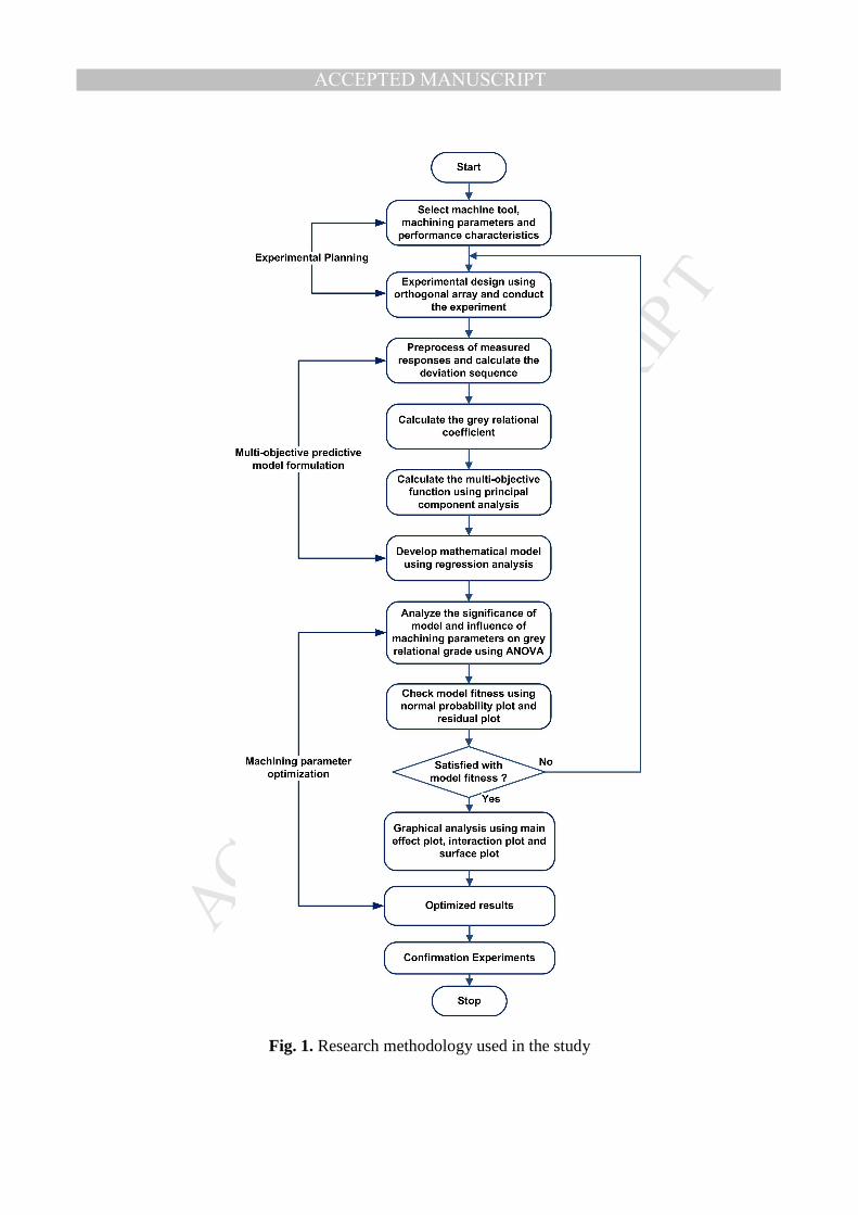
The research carried out for this paper can be broadly divided into three phase –

experimental planning; multi-objective predictive model formulation; and machining parameters

optimization – followed by result confirmation using experimental studies as shown in Fig. 1.

Insert Figure 1 here

In the first phase experimental plan was developed to select the machine tool, cutting

tools, machining material, machining parameters and their levels, and performance

characteristics (power consumption and surface roughness). Experiments were designed using

full factorial L27 orthogonal array through well known Taguchi method. Full array was selected

to get a wider range of experimental data. Next, machining experiments were conducted for the

MANUSCRIP

T

ACCEPTED

ACCEPTED MANUSCRIPT

10

27 combinations of orthogonal array to get the power consumption and surface roughness data.

In the second phase, GRA coupled with principal component analysis (PCA) has been used to

determine the best combination of parameters. GRA converts the multi-objective problem

(power consumption and surface roughness) into a single multi-objective function (grey

relational grade); and hence simplifies the optimization procedure. Principal component analysis

has been used to determine the weights of power consumption and surface roughness in the

multi-objective function. Next, a mathematical model was developed to predict the relationship

between machining parameters and grey relational grade using regression analysis. In the third

phase, the statistical significance of the developed model was analyzed using analysis of variance

(ANOVA). The fitness of developed model was checked using normal probability plot and

residual plot. The influence of machining parameters on multi-objective function (grey relational

grade) was determined using main effect and interaction plots. Response surface contours were

constructed for determining a range of optimum conditions for required power consumption and

surface roughness conditions. Lastly, experimental tests were carried out at the optimum

machining parameters to confirm the results.

3.2 Analysis Methods

This research uses the three methodologies to analyze the experimental data – response surface

methodology, grey relational analysis and principal component analysis. An overview of these

methodologies is provided here.

3.2.1 Response surface methodology

Engineering experiments aim at determining the conditions that can lead to optimum

performances. One of methodologies for obtaining the optimum performance is RSM. RSM was

MANUSCRIP

T

ACCEPTED

ACCEPTED MANUSCRIPT

11

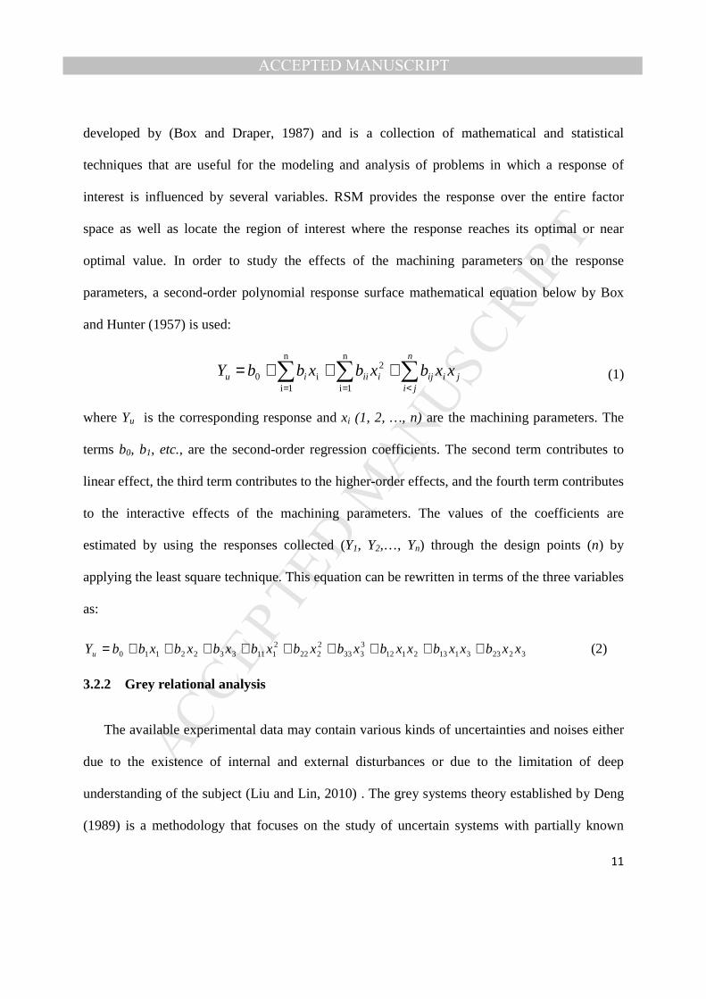
developed by (Box and Draper, 1987) and is a collection of mathematical and statistical

techniques that are useful for the modeling and analysis of problems in which a response of

interest is influenced by several variables. RSM provides the response over the entire factor

space as well as locate the region of interest where the response reaches its optimal or near

optimal value. In order to study the effects of the machining parameters on the response

parameters, a second-order polynomial response surface mathematical equation below by Box

and Hunter (1957) is used:

2n

1ii

n

1i0 ji

n

jiijiiiiu xxbxbxbbY ∑∑∑

<==

+++= (1)

where Yu is the corresponding response and xi (1, 2, …, n) are the machining parameters. The

terms b0, b1, etc., are the second-order regression coefficients. The second term contributes to

linear effect, the third term contributes to the higher-order effects, and the fourth term contributes

to the interactive effects of the machining parameters. The values of the coefficients are

estimated by using the responses collected (Y1, Y2,…, Yn) through the design points (n) by

applying the least square technique. This equation can be rewritten in terms of the three variables

as:

3223311321123333

2222

21113322110 xxbxxbxxbxbxbxbxbxbxbbYu +++++++++= (2)

3.2.2 Grey relational analysis

The available experimental data may contain various kinds of uncertainties and noises either

due to the existence of internal and external disturbances or due to the limitation of deep

understanding of the subject (Liu and Lin, 2010) . The grey systems theory established by Deng

(1989) is a methodology that focuses on the study of uncertain systems with partially known

MANUSCRIP

T

ACCEPTED

ACCEPTED MANUSCRIPT

12

information through generating, excavating, and extracting useful information from available

data. In grey systems theory, white indicate complete information, black unknown information

and grey partially known and partially unknown information (Liu and Lin, 2010). Machining is

known as one of the most complex system due to large variety of machining operations, input

and output variables, work material properties, and complex tool/work material interface (van

Luttervelt et al., 1998). Therefore, grey system theory has a wide range of applicability in

machining operations. The grey relational analysis consists of following steps (Tzeng et al.,

2009).

Data preprocessing

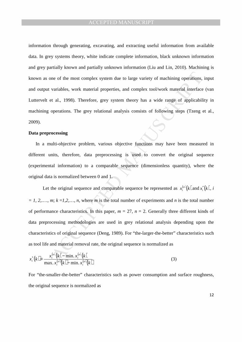
In a multi-objective problem, various objective functions may have been measured in

different units, therefore, data preprocessing is used to convert the original sequence

(experimental information) to a comparable sequence (dimensionless quantity), where the

original data is normalized between 0 and 1.

Let the original sequence and comparable sequence be represented as ( )( )kx oi and ( )kxi

*, i

= 1, 2,.…, m; k =1,2,…, n, where m is the total number of experiments and n is the total number

of performance characteristics. In this paper, m = 27, n = 2. Generally three different kinds of

data preprocessing methodologies are used in grey relational analysis depending upon the

characteristics of original sequence (Deng, 1989). For “the-larger-the-better” characteristics such

as tool life and material removal rate, the original sequence is normalized as

( )( ) ( ) ( ) ( )

( ) ( ) ( ) ( )kxkx

kxkxkx

oi

oi

oi

oi

i min. max.

min. *

−−

= (3)

For “the-smaller-the-better” characteristics such as power consumption and surface roughness,

the original sequence is normalized as

MANUSCRIP

T

ACCEPTED

ACCEPTED MANUSCRIPT

13

( )( )( ) ( ) ( )

( ) ( ) ( )( )kxkx

kxkxkx

oi

oi

oi

oi

i min. max.

max. *

−−

= (4)

For “a specific desired value”, the original sequence is normalized as

( )( ) ( )

( )( ) ( )( ){ }kxkx

kxkx

oi

oi

oi

i min. OD OD, max. .max

OD 1 *

−−

−−= (5)

where OD is the desired value.

Grey relational coefficients

After data processing, a grey relational coefficient is calculated with the preprocessed sequences.

The grey relational coefficient is defined as:

( ) ( )( ) ( ) .max0

.maxmin.**0

,

∆+∆∆+∆

=ζ

ζγk

kxkxi

i (6)

( ) ( )( ) 1 , 0 **0 ≤< kxkx iγ

where ( )ki0∆ is the deviational sequence of reference sequence ( )kx*0 and comparability

sequence ( )kxi*

, i.e. ( ) ( ) ( )kxkxk ii**

00 −=∆ is the absolute value of the difference between ( )kx*0

and ( )kxi* .

( )kik

0i

min .min min. ∆=∆∀∀

( )kik

0i

max .max max. ∆=∆∀∀

ζ is the distinguish coefficient. [ ]0,1 ∈ζ .

Grey relational grade

The grey relational grade is a weighted sum of the grey relational coefficients. It is defined as

follows:

MANUSCRIP

T

ACCEPTED

ACCEPTED MANUSCRIPT

14

( ) ( ) ( )( )kxkxxx i

n

kki

**0

1

**0 , , ∑

=

= γβγ (7)

∑=

=n

kk

1

1 β

where kβ denotes the weighted value of the kth response variable. In this study, the weights are

obtained from the principal component analysis.

The grey relational grade ( )**0 , ixxγ represents the level of correlation between the

reference and comparability sequence. It is a measurement of the absolute value of data

difference between two sequences and can be used to approximate the correlation between the

sequences. The value of grey relational grade is equal to one, if the two sequences are identical.

It indicates the degree of influence that the comparability sequence could exert over the reference

sequence.

3.2.3 Principal component analysis

Principal component analysis is the oldest and one of the best known techniques of multivariate

analysis. It was first introduced by Pearson in 1901 and developed independently by Hotelling

in 1933 (Jolliffe, 2002). It is a technique of dimensionality reduction, which transforms data

from the high-dimensional space to space of lower dimensions. It rotates the axes of data space

along lines of maximum variance. The axis of the greatest variance is called the first principal

component (Sanguansat, 2012). The dimension reduction is done by using only the first few

principal components as a basis set for the new space. Therefore, the subspace tends to be small

and may be dropped with minimal loss of information. PCA has the following advantages

(Sanguansat, 2012).

MANUSCRIP

T

ACCEPTED

ACCEPTED MANUSCRIPT

15

• Retains most of the useful information and reduces noise and other undesirable artifacts.

• The time and memory used in data processing are smaller.

• Provides a way to understand and visualize the structure of complex data sets.

• Helps to identify new meaningful underlying variables.

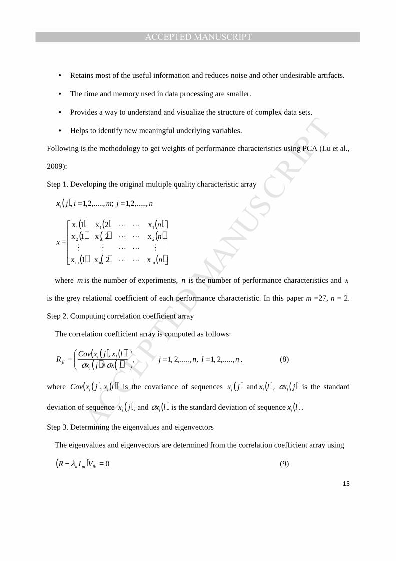
Following is the methodology to get weights of performance characteristics using PCA (Lu et al.,

2009):

Step 1. Developing the original multiple quality characteristic array

( ) njmijxi ,.....,2,1 ;,.....,2,1 , ==

( ) ( )( ) ( )

( ) ( )

( )( )

( )

=

n

n

n

x

m

2

1

mm

22

11

x

x

x

2x1x

2x1x

2x1x

M

LL

LLMM

LL

LL

where mis the number of experiments, n is the number of performance characteristics and x

is the grey relational coefficient of each performance characteristic. In this paper m =27, n = 2.

Step 2. Computing correlation coefficient array

The correlation coefficient array is computed as follows:

( ) ( )( )( ) ( )

×=

lxjx

lxjxCovR

ii

iijl σσ

,, nlnj ,.....,2 ,1 ,,.....,2 ,1 == , (8)

where ( ) ( )( )lxjxCov ii , is the covariance of sequences ( )jxi and ( )lxi , ( )jxiσ is the standard

deviation of sequence ( )jxi , and ( )lxiσ is the standard deviation of sequence( )lxi .

Step 3. Determining the eigenvalues and eigenvectors

The eigenvalues and eigenvectors are determined from the correlation coefficient array using

( ) 0=− ikmk VIR λ (9)

MANUSCRIP

T

ACCEPTED

ACCEPTED MANUSCRIPT

16

where kλ is the eigenvalues and nn

kk =∑

=1

λ , [ ]Tkmkkik aaaVnk ........ ,,.....,2 ,1 21== are the

eigenvectors corresponding to the eigenvalue kλ .

Step 4. Finding principle components

The uncorrelated principal component is formulated as:

( ) ik

n

immk VixY ⋅=∑

=1

(10)

where 1mY is the first principal component, 2mY is the second principal component and so on. The

principal components are aligned in the descending order with respect to variance. The

components with an eigenvalue greater than one are chosen to replace the original responses for

further analysis (Kaiser, 1960) .

4. Experimental Planning

4.1 Selecting machining parameters and performance characteristics

The turning experiments were carried out in dry cutting conditions using a centre lathe,

which has a maximum spindle speed of 2300 rpm and a spindle power of 5.5 kW. For increasing

rigidity of the machining system, workpiece material was held between chuck and tailstock and

the tool overhang was 20 mm. The choice of machining parameters was made by taking into

account the capacity/limiting cutting conditions of the lathe, tool manufacturer’s catalogue and

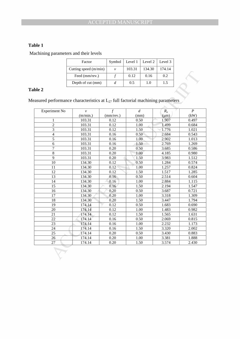
the values taken by researchers in the literature. Table 1 provides the three machining parameters

and the three levels for each parameter.

Insert Table 1 here

MANUSCRIP

T

ACCEPTED

ACCEPTED MANUSCRIPT

17

Material

The sample material for the research was AISI 1045 steel in the form of cylindrical shape

with 47 mm diameter and 250 mm cutting length.

Cutting tool inserts and holder

Uncoated tungsten carbide tools were used. The cutting tool used is proper for machining of

AISI 1045 steel with ISO P25 quality. Sandvik inserts with the ISO TNMG 16 04 12 designation

were mounted on the tool holder designated by ISO as PTGNR 2020 K16 having rake angle of

+7 degree, clearance angle of +6 degree and 0.4 mm nose radius.

4.3 Performance parameter measurement

A pre-cut of 1 mm depth was performed on each workpiece prior to actual turning using a

different cutting tool. This was done in order to remove the rust or hardened top layer from the

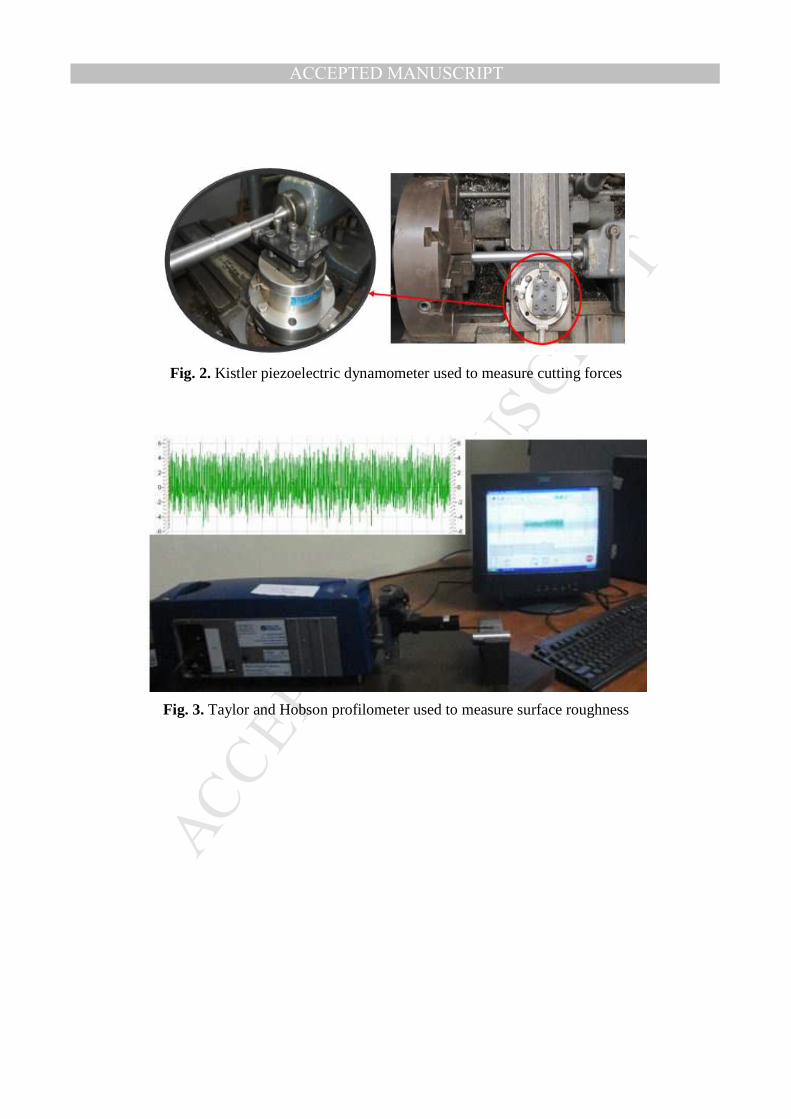
outside surface and to minimize any effect of non-homogeneity on the experimental results. An

indirect method of power measurement by measuring cutting forces is used to measure the power

consumed during machining. Kistler Type 9272 dynamometer shown in Fig. 2, connected to a

multichannel charge amplifier (Type 5070A) by a highly insulated connection cable, was used to

measure three force components (cutting force, feed force and radial force). The amplifier

amplifies the electrical charges delivered from the dynamometer into proportional voltages and

then the proportional forces were processed using Dynoware software package.

Insert Figure 2 here

MANUSCRIP

T

ACCEPTED

ACCEPTED MANUSCRIPT

18

After each test, once the cut for a specified time was over, the roughness of the finished

surface was measured by placing the workpiece on a V-block over a granite surface plate. Each

value was measured at three equally spaced locations around the circumference of the workpiece

to obtain the statistically significant data for test and then the mean of measurements was

calculated. Thus, probable observation errors were kept relatively small. Taylor and Hobson

make profilometer, shown in Fig. 3, is used for measuring the surface roughness. The equipment

was calibrated by measuring the known diameter of a high precision spherical ball. The

Taguchi’s L27 orthogonal array was used to obtain the experimental data. The experimental

combinations of machining parameters and the corresponding measured power consumption (P)

and surface roughness (Ra) are given in Table 2.

Insert Figure 3 here

Insert Table 2 here

5. Formulation of a multi-objective predictive mathematical model

5.1 Calculating the grey relation co-efficient using GRA

The experimental results for the Ra and P are listed in Table 2. Preprocessing sequence

(Table 3) was computed using Eq. (4) as both surface roughness and power consumption fit ‘the-

smaller-the-better’ methodology. ( )kx*0 shows the value for reference sequence and ( )kxi

* for

comparability sequence. The deviation sequence is computed using:

( ) ( ) ( ) 2220.07780.00000.1 **001 =−=−=∆ aiaa RxRxR

MANUSCRIP

T

ACCEPTED

ACCEPTED MANUSCRIPT

19

( ) ( ) ( ) 0000.00000.10000.1 **001 =−=−=∆ PxPxP i

Therefore the value of deviation sequence for comparability sequence one in Table 3 is:

( )0000.2220,0.0 01 =∆

Similarly, the deviation sequences for other comparability sequences were computed and the

values are shown in Table 3. Values of max∆ and min∆ are computed as:

( ) ( ) 0000.121 02708max =∆=∆=∆

( ) ( ) 0000.021 01011min =∆=∆=∆

Insert Table 3 here

The grey relational coefficient values using Eq. (6) are computed as:

( ) ( )( ) ( ) 6925.01.0000 .50 .22200

1.0000 .50 .00000

1

1 ,1

.max01

.maxmin.*1

*0 =

×+×+=

∆+∆∆+∆

=ζζγ xx

( ) ( )( ) ( ) 0000.11.0000 .50 .00000

1.0000 .50 .00000

2

2 ,2

.max01

.maxmin.*1

*0 =

×+×+=

∆+∆∆+∆

=ζ

ζγ xx

Therefore, ( ) ( )( ) ( )0000.1 ,6925.0 , **0 =PxRx iaγ

The same procedure was performed to get the grey relational coefficients for other comparability

sequences and values are shown in Table 3.

5.2 Computing grey relation grade

The next step is to compute grey relational grade which is a weighted sum of the grey

relational coefficients using Eq. (7). The computation of grey relational grade also requires

weights of the performance characteristics for which eigenvalues and eigenvectors are required.

MANUSCRIP

T

ACCEPTED

ACCEPTED MANUSCRIPT

20

Grey relational coefficient values shown in Table 3 are further used to evaluate the

corresponding coefficient matrix using Eq. (8). Eigenvalues, eigenvectors and corresponding

principal components are computed using Eq. (9) and Eq. (10) and shown in Table 4 and Table

5.

Insert Table 4 here

Insert Table 5 here

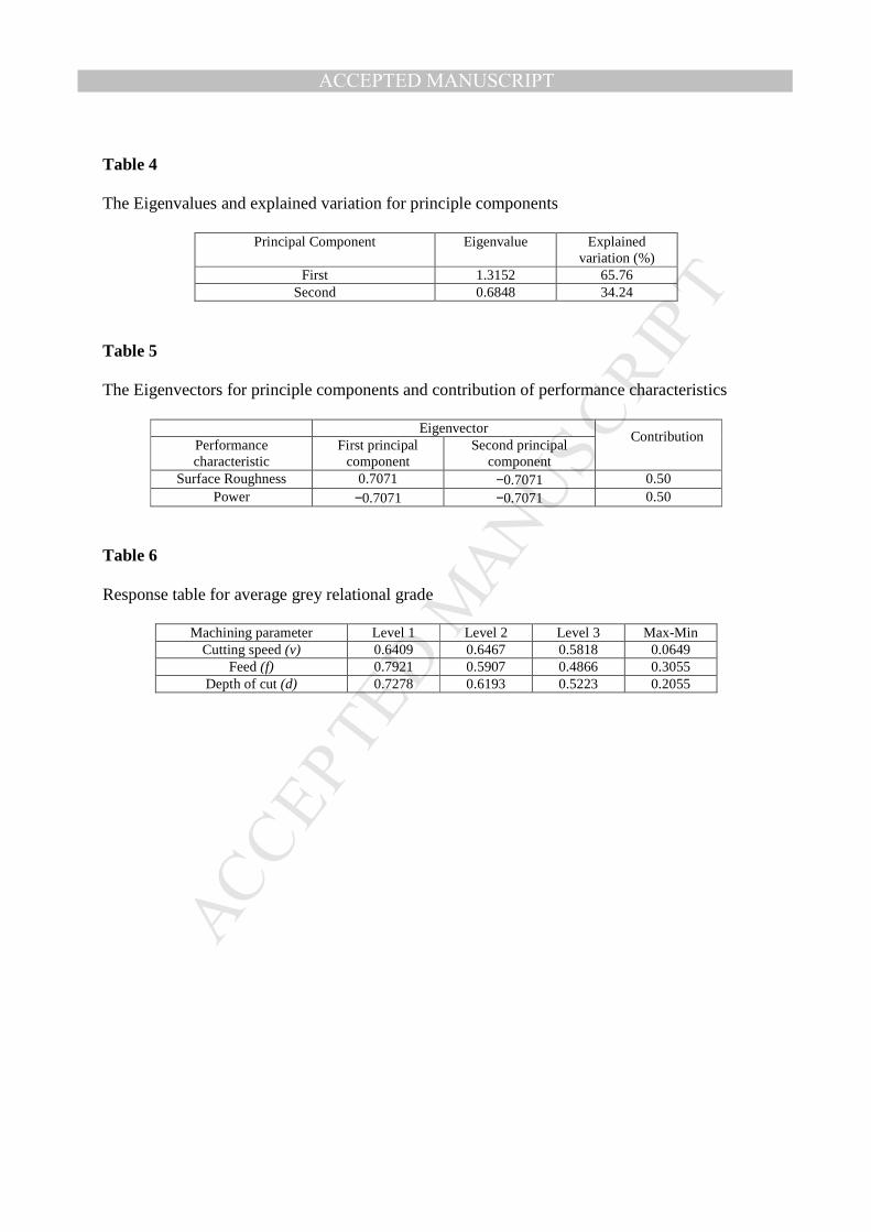
The variance contribution shown in Table 4 for the first principal component characterizing the

two performance characteristics is as high as 65.76%. The square of eigenvector can represent

the contribution of corresponding performance characteristic to the principle component.

Therefore, in this analysis, the square of eigenvector of first principle component was selected as

the weighting values of the related performance characteristic. Table 5 shows the weighting

value (contribution) of Ra and P. The equal weighting values of ‘Ra’ and ‘P’ clearly show that

the power consumption is as important as surface roughness for a machine tool. Therefore, the

coefficients, 1β and 2β in Eq. (6) were set as 0.5 and 0.5. Based on Eq. (6) and the data listed in

Table 3, the grey relational grade ( )**0 , ixxγ can be computed as follows:

( ) 8463.0500 0000.1 500 6925.0 , **0 =×+×= ..xx iγ

The grey relational grades for other 26 experimental values were calculated using above

methodology. The values are given in the last column of Table 3. Therefore, the optimization of

performance characteristics can be performed with respect to single grey relational grade rather

MANUSCRIP

T

ACCEPTED

ACCEPTED MANUSCRIPT

21

than multiple performance characteristics. This grey relation grade is a multi-objective function

integrating surface roughness and power consumption.

5.3 Finding best experimental run

The Taguchi method has been used to calculate the average grey relational grade for each

machining parameter level. It has been done by sorting the grey relational grades corresponding

to levels of the machining parameter in each column of the orthogonal array and taking an

average at the same level. The average grey relation grade for 1v is computed as follows:

( )6409.0

9

4186.05001.06459.05239.05614.07305.06934.08480.08463.01 =++++++++=v

Similarly, the average grey relational grade values for v, f and d at the three levels are computed

and given in Table 6.

Insert Table 6 here

The larger the grey relational grade, the better the corresponding performance

characteristics. Accordingly, the level that gives the largest average response is best. Thus, the

optimal levels of each parameter are the cutting speed at level 2 (134.3 m/min), feed at level 1

(0.12 mm/rev.) and depth of cut at level 1 (0.5 mm). Furthermore, the Max-Min value, which is

difference between the maximum and minimum value for each cutting parameter is calculated as

shown in Table 6. The Max-Min value of feed is maximum. Depth of cut and cutting speed are at

the second and third place respectively. It indicates that feed has the maximum influence on

average grey relational grade while cutting speed has the minimum influence.

MANUSCRIP

T

ACCEPTED

ACCEPTED MANUSCRIPT

22

5.4 Predictive mathematical formulation

The mathematical model for the grey relational grade prediction is developed using regression

analysis based on the grey relational grade values obtained. The developed predictive

mathematical model for grey relational grade is:

)0.157500 30.00031857 00274287.0 0230667.0 30.3958

0000256225.0 182721.0 0110.13 00703258.0 .718311(

Maximize

22

2

fdvdvfdf

vdfv

−−−++−−−+ (11)

Constraints : 103.31 m/min ≤ v ≤ 174.14 m/min

0.12 mm/rev. ≤ f ≤ 0.16 mm/rev.

0.5 mm ≤ d ≤ 1.5 mm

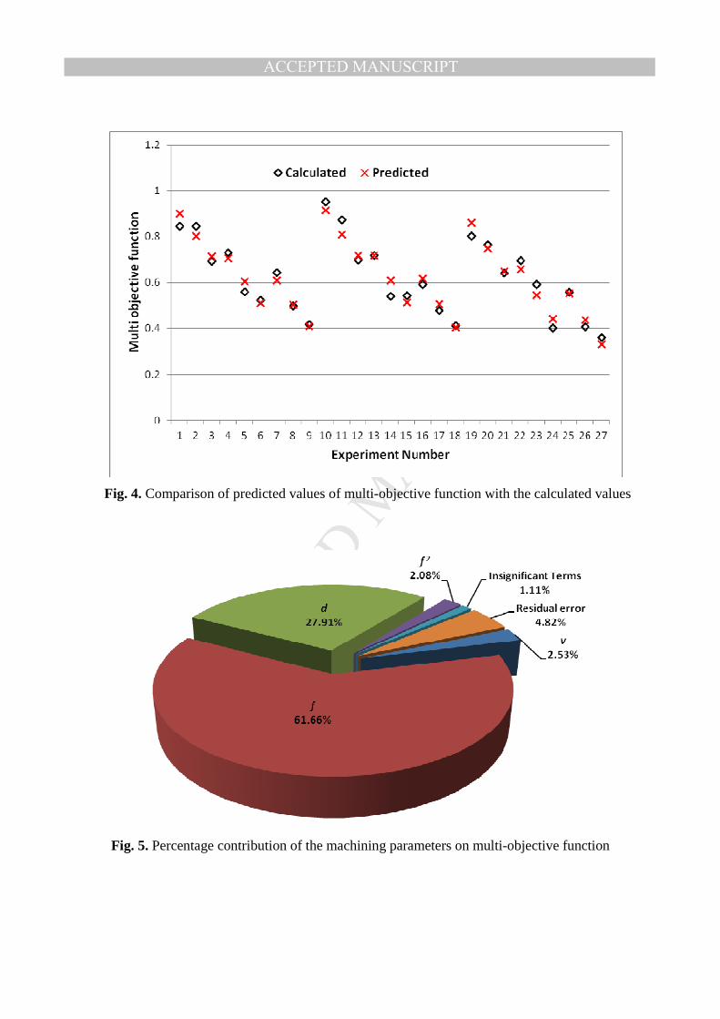
Fig. 4 shows the predicted values of grey relational grade, hereafter called multi-objective

function from the developed mathematical model and the calculated values of Table 3 obtained

using GRA. Both values are in good agreement to each other. The mean relative error between

the both values is 4.79%.

Insert Figure 4 here

6. Machining parameter optimization

6.1 Analysis of variance

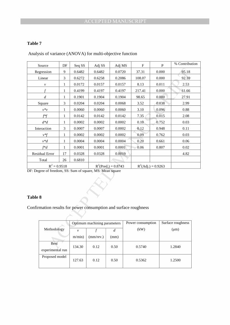
The relative importance among the machining parameters (v, f, d) for the multiple

performance characteristics (Ra and P) needs to be investigated so that the optimal parameters

can be decided effectively. The analysis of variance (ANOVA) has been applied to investigate

the developed model and the effect of machining parameters on the multi-objective function.

Table 7 shows ANOVA results for the linear [v, f, d,] quadratic [v 2, f 2, d2] and interactive [(v×f),

MANUSCRIP

T

ACCEPTED

ACCEPTED MANUSCRIPT

23

(v×d), (f×d)] factors. F-value, which is a ratio of the regression mean square to the mean square

error, is used to measure the significance of the model under investigation with respect to the

variance of all the terms including the error term at the desired significance level. Usually, F>4

means the change of the design parameter has a significant effect on the performance

characteristic. The F-value for linear terms is above 4. P-value or probability value is used to

determine the statistical significance of results at a confidence level. In this study the

significance level of α = 0.05 is used, i.e. the results are validated for a confidence level of 95%.

If the P-value is less than 0.05 then the corresponding factor has a statistically significant

contribution to the performance characteristic and if the P-value is more than 0.05 then it means

the effect of factor on the performance characteristic is not statistically significant at 95%

confidence level. The results show that all linear terms and f 2 are statistically significant at 95%

level. The last column of the Table 7 shows the percentage contribution of each source to the

total variation indicating the degree of influence on the results.

Insert Table 7 here

The percentage contribution of each term is also shown in Fig. 5. Feed (f) was found to be the

most significant machining parameter due to its highest percentage contribution of 61.66%

followed by the depth of cut (d) with 27.91% and cutting speed (v) with 2.53%. However, the

percentage contribution of quadratic term f 2 is 2.08%. The other quadratic and interaction terms

are insignificant.

Insert Figure 5 here

MANUSCRIP

T

ACCEPTED

ACCEPTED MANUSCRIPT

24

The other important coefficient is R2, which is defined as the ratio of the explained variation

to the total variation and is a measure of the degree of fit. As R2 approaches unity, the response

model fitness with the actual data improves. The value of R2 obtained was 0.9518 which

indicates that 95.18% of the total variations are explained by the model. The adjusted R2 is a

statistic that is adjusted for the “size” of the model, i.e. the number of factors. The value of the

R2 (Adj.) = 0.9263 indicating 92.63% of the total variability is explained by the model after

considering the significant factors. R2 (Pred.) = 87.43% is in good agreement with the R2 (Adj.)

and shows that the model is expected to explain 87.43% of the variability in any new data.

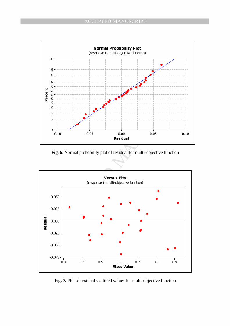
6.2 Model fitness check

The adequacy of the modal has been investigated by the examination of residuals. The

residual, which is the difference between the respective observed response and the predicted

response, is examined using normal probability plots and the plots of the residual versus the

predicted response as shown in Fig. 6 and Fig. 7 respectively. If the model is adequate, the points

on the normal probability plots of the residual should form a straight line. Fig. 6 reveals that the

residuals are not showing any particular trend and the errors are distributed normally. The

residual versus the predicted response plot in Fig. 7 also shows that there is no obvious pattern

and unusual structure. This suggests the adequacy of the developed model for evaluating the

multi-objective function.

Insert Figure 6 here

MANUSCRIP

T

ACCEPTED

ACCEPTED MANUSCRIPT

25

Insert Figure 7 here

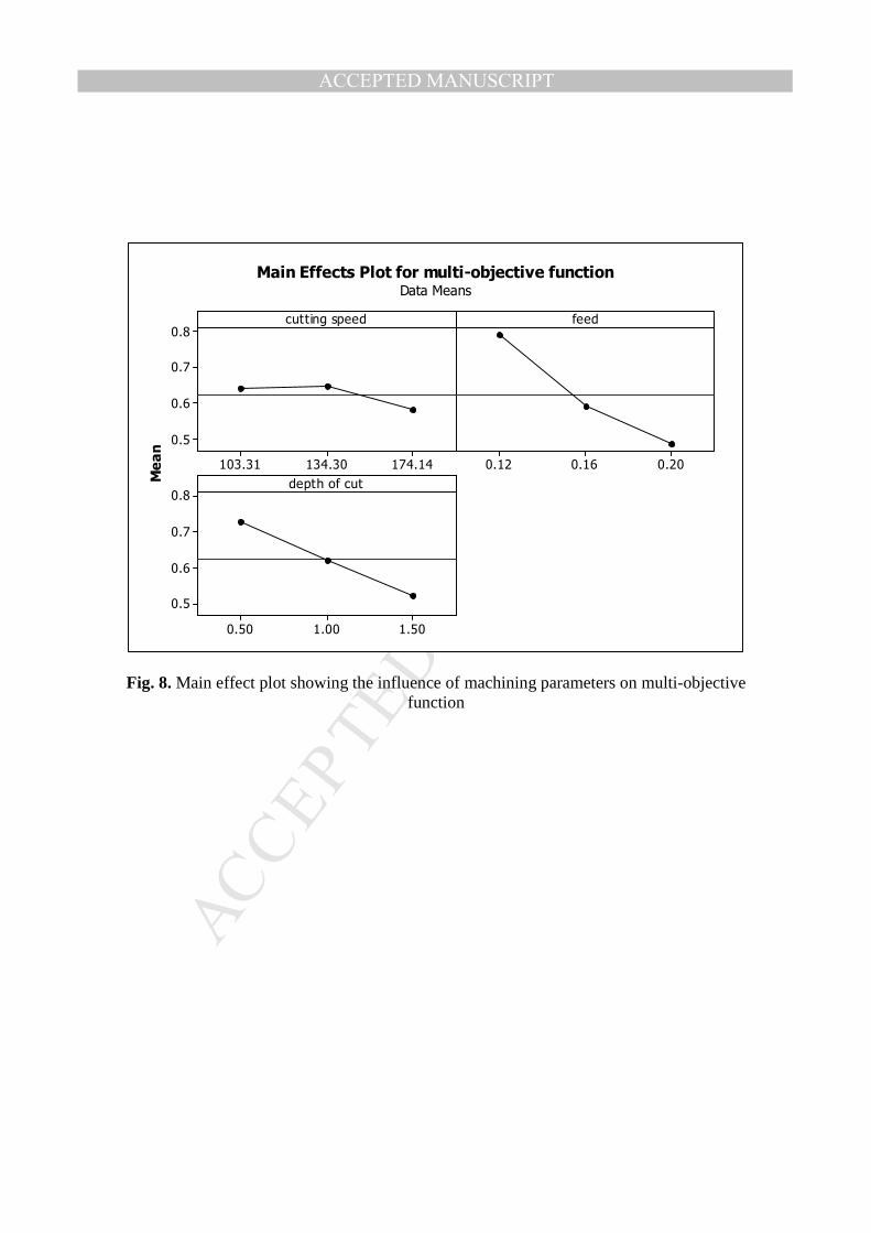
6.3 Parametric influence on multi-objective function

The main effects plot of machining parameters versus multi-objective function is shown in

Fig. 8. The slope of feed and depth of cut is large which shows that both have more impact on

multi-objective function (power consumption and surface roughness). The cutting speed has

almost negligible impact on multi-objective function. This trend is also supported by the

percentage contribution values in the ANOVA results in Table 7. Main effect plot clearly shows

that the multi-objective function will be maximum, when the values of feed and depth of cut are

smaller. Therefore, to get the better surface finish at minimum power consumption, the

recommended values are level 1 for feed and depth of cut and level 2 for cutting speed. The

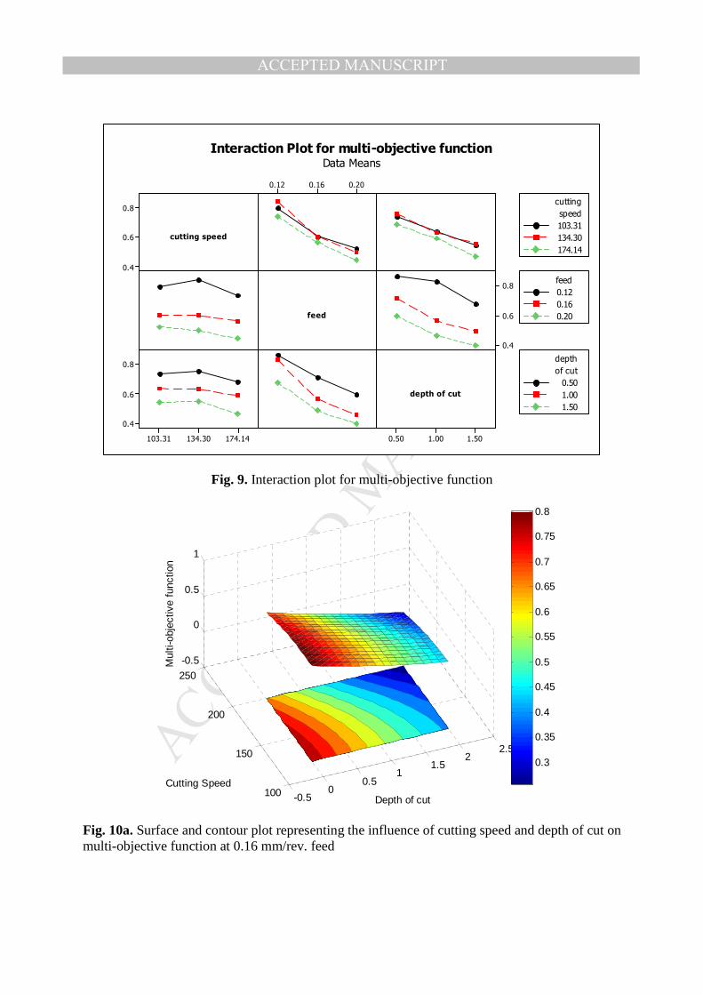
interaction plot for mean multi-objective function is shown in Fig. 9. This figures clearly shows

that the variation of cutting speed has low effect on the multi-objective function for both feed

and depth of cut variation as the spacing between the lines is small (row 1 column 2 for feed and

row 1 and column 3 for depth of cut). The variation of multi-objective function is high with

variation of feed and depth of cut (row 2 and column 3) as the multi-objective function value is

approximately 0.4 for level 3 feed and level 3 depth of cut, and this value is approximately 0.9

for level 1 of feed and depth of cut.

Insert Figure 8 here

Insert Figure 9 here

The 3D merged surface and contour plots for the multi-objective function are shown in Fig

10. Fig. 10a shows the surface and contour plots for multi-objective function with respect to

MANUSCRIP

T

ACCEPTED

ACCEPTED MANUSCRIPT

26

varying cutting speed and depth of cut at a fixed feed. It shows that at smaller values of cutting

speed and depth of cut, the multi-objective function is maximum and decreases with increase in

depth of cut even at smaller value of cutting speed. It again supports this observation that depth

of cut has more influence on multi-objective function as compared to cutting speed. Fig. 10b

shows the surface and contour plots for multi-objective function with respect to varying cutting

speed and feed at a fixed depth of cut. It reveals that at the smaller values of feed, the multi-

objective function is maximum. Even with increase in cutting speed at smaller values of feed the

multi-objective function is maximum and at higher values of feed it decreases. Fig. 10c indicates

that multi-objective function is maximum at lower values of depth of cut and feed and minimum

at larger values of depth of cut and feed. These 3D surface plots can be used for estimating the

power consumption and surface roughness values for any suitable combination of the machining

parameters, namely cutting speed, feed and depth of cut. This is very useful in practice for the

operator or part programmer.

Insert Figure 10a here

Insert Figure 10b here

Insert Figure 10c here

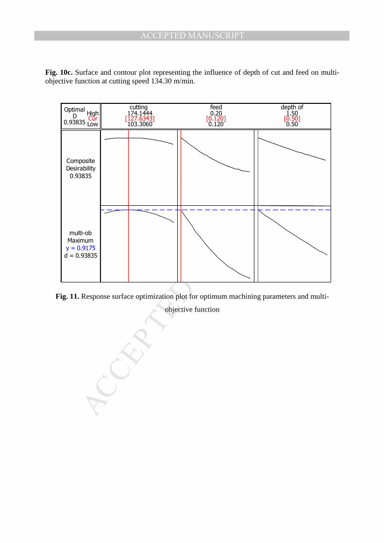
6.4 Optimum values of multi-objective function

One of the objectives of this study was to find the optimum values of machining parameters

to achieve the minimum power consumption and surface roughness. The response surface

optimization is an ideal technique for determination of these optimum machining parameters.

Response surface optimization was done using MINITAB and the results are shown in Fig. 11.

The optimal machining parameters for minimizing surface roughness and power consumption

MANUSCRIP

T

ACCEPTED

ACCEPTED MANUSCRIPT

27

obtained are – cutting speed of 127.63 m/min at feed rate of 0.12 mm/rev with 0.50 mm depth of

cut.

Insert Figure 11 here

7. Confirmation experiments

The confirmation experiments were conducted on the optimal machining parameters (v =

127.63 m/min, f = 0.12 mm/rev and d = 0.50 mm) predicted using the developed model. The

result of the confirmation runs for the power consumption and surface roughness are listed in

Table 8. It can be observed that the optimal machining parameters predicted by the developed

model will lead to lower power consumption and better surface roughness as shown in Table 8.

Insert Table 8 here

8. Discussion

8.1 The influence of machining parameters on power consumption and surface

roughness

Machine tools consume power to provide the relative movement to the cutting tool with

respect to the workpiece and rotation of spindle. The three machining parameters, viz. cutting

speed, feed and depth of cut determine the material removal rate. As the feed and depth of cut

increases, the undeformed chip section increases and hence the force required to remove this area

also increases which forces the machine tool to consume more power. The surface roughness

also increases with increase in feed. It is quite obvious because for a given tool nose radius the

MANUSCRIP

T

ACCEPTED

ACCEPTED MANUSCRIPT

28

theoretical surface roughness; Ra ≈ f 2/ 8r, where f is feed and r is nose radius of the cutting tool;

is a function of feed (Shaw, 1984). This situation can be explained as the increase in feed leads to

vibration and more heat generation and therefore contributes to higher surface roughness

(Sarıkaya and Güllü, 2014). In actual practice, build-up edge formation and vibration (chatter)

are the major factors affecting surface quality. An increase in cutting speed reduces the

possibility of built-up edge formation and hence improves the surface quality. This result

supports the argument that high cutting speeds reduce cutting forces together with the effect of

natural frequency and vibration, giving better surface finish (Cakir et al., 2009). The better

surface quality with least power consumption can be achieved at lower feed and depth of cut.

8.2 Comparative benefits between proposed model and literature models

This paper optimizes power consumption and surface roughness simultaneously during a

turning operation on AISI 1045. The authors were able to find only one research paper (Hanafi et

al, 2012) which provides simultaneous optimization of power and surface roughness during

turning operation but on a composite material. Hanafi et al (2012) used GRA and Taguchi

optimization methodology to optimize power consumption and surface roughness for poly-

etheretherkeytone material. The obtained results revealed that depth of cut is the most influential

parameters and feed rate is the least influential parameter. The current research shows that feed

rate is the most significant factor and cutting speed is least significant. This difference may be

because of difference in the workpiece material. However, the results of Camposeco-Negrete

(2013) while working on AISI 6061 T6 material demonstrated that feed is the most significant

factor and cutting speed is the least significant parameter for minimizing the total power

consumption. Abhang and Hameedullah (2010) also demonstrated the feed rate has the most

significant effect on power consumption, followed by depth of cut, tool nose radius and cutting

MANUSCRIP

T

ACCEPTED

ACCEPTED MANUSCRIPT

29

speed during machining of the turning of EN-31 steel with tungsten carbide tool. Cetin et al.

(2011) also indicated that the effects of feed rate and depth of cut are more effective than cutting

spindle speed on reducing the forces and improving the surface finish. Moreover, theoretically as

well as experimentally it is well known that feed rate has the maximum influence on surface

roughness during the machining of metals.

The proposed model does not assume the weights of the two factors, viz. power

consumption and surface roughness, but determines the weights of the factors using principal

component analysis. Hanafi et al (2012) have assumed the weights of the two factors.

The RSM technique used in this paper can model the response in terms of significant

parameters, their interactions and square terms. 3D surfaces generated by RSM can help in

visualizing the effect of parameters on response in the entire range specified whereas Taguchi’s

technique used by Emami et al. (2014), Camposeco-Negrete (2013), Hanafi et al (2012), etc

gives the average value of response at given level of parameters.

In this paper the mean relative error between the experimental and predicted data is 4.79%

and is well in agreement with the results from literature. The mathematical model developed

using RSM by the Sarıkaya and Güllü (2014) shows that the percentage deviation between the

experimental data and prediction data is between 2.72% and 7.14%.

Conclusions This paper presents a multi-objective predictive model for the minimization of power

consumption and surface roughness during the machining of AISI 1045 steel. It has been

observed that the predictive model provides optimum machining parameters. The predictive

model has been found statistically significant using ANOVA. The results of the proposed model

MANUSCRIP

T

ACCEPTED

ACCEPTED MANUSCRIPT

30

provide an improvement of 6.59% reduction in power consumption and 2.65% improvement in

surface roughness over the best experimental run. It has been observed that the feed is the main

influencing machining parameter for the minimization of power consumption and surface

roughness followed by the depth of cut and cutting speed. The 3D surface and contour plots

constructed during the study can be used for choosing the optimal machining parameters to

obtain particular values of power consumption and surface roughness or vice-versa these can be

used by the machine tool manufacturers to provide the range of cutting speeds, feed and depth of

cut for the particular application. This work can be further extended to analyze the effect of

different cutting conditions and cutting tools on power consumption and surface roughness

during machining.

References

Abhang, L.B., Hameedullah, M., 2010. Power Prediction Model for Turning EN-31 Steel Using Response Surface Methodology. J. Eng. Sci. Technol. Rev. 3, 116–122.

Aggarwal, A., Singh, H., Kumar, P., Singh, M., 2008. Optimizing power consumption for CNC turned parts using response surface methodology and Taguchi’s technique—A comparative analysis. J. Mater. Process. Technol. 200, 373–384.

Arrazola, P.J., Umbrello, D., Davies, M., Jawahir, I.S., 2013. Recent advances in modelling of metal machining processes. CIRP Ann. - Manuf. Technol. 62, 695–718.

Bhattacharya, A., Das, S., Majumder, P., Batish, A., 2009. Estimating the effect of cutting parameters on surface finish and power consumption during high speed machining of AISI 1045 steel using Taguchi design and ANOVA. Prod. Eng. 3, 31–40.

Bhushan, R.K., 2013. Optimization of cutting parameters for minimizing power consumption and maximizing tool life during machining of Al alloy SiC particle composites. J. Clean. Prod. 39, 242–254.

Box, G., Draper, N., 1987. Empirical model-building and response surface, Empirical model-building and. John Wiley & Sons, New York.

MANUSCRIP

T

ACCEPTED

ACCEPTED MANUSCRIPT

31

Box, G.E.P., Hunter, J.S., 1957. Multi-Factor Experimental Designs for Exploring Response Surfaces. Ann. Math. Stat. 28, 195–241.

Cakir, M.C., Ensarioglu, C., Demirayak, I., 2009. Mathematical modeling of surface roughness for evaluating the effects of cutting parameters and coating material. J. Mater. Process. Technol. 209, 102–109.

Campatelli, G., Lorenzini, L., Scippa, A., 2014. Optimization of process parameters using a Response Surface Method for minimizing power consumption in the milling of carbon steel. J. Clean. Prod. 66, 309–316.

Camposeco-Negrete, C., 2013. Optimization of cutting parameters for minimizing energy consumption in turning of AISI 6061 T6 using Taguchi methodology and ANOVA. J. Clean. Prod. 53, 195–203.

Cetin, M.H., Ozcelik, B., Kuram, E., Demirbas, E., 2011. Evaluation of vegetable based cutting fluids with extreme pressure and cutting parameters in turning of AISI 304L by Taguchi method. J. Clean. Prod. 19, 2049–2056.

Deng Julong, 1989. Introduction to Grey System Theory. J. Grey Syst. 1, 1–24.

Emami, M., Sadeghi, M.H., Sarhan, A.A.D., Hasani, F., 2014. Investigating the Minimum Quantity Lubrication in grinding of Al2O3 engineering ceramic. J. Clean. Prod. 66, 632–643.

Fang, K., Uhan, N., Zhao, F., Sutherland, J.W., 2011. A new approach to scheduling in manufacturing for power consumption and carbon footprint reduction. J. Manuf. Syst. 30, 234–240.

Fratila, D., Caizar, C., 2011. Application of Taguchi method to selection of optimal lubrication and cutting conditions in face milling of AlMg 3. J. Clean. Prod. 19, 640–645.

Hanafi, I., Khamlichi, A., Cabrera, F.M., Almansa, E., Jabbouri, A., 2012. Optimization of cutting conditions for sustainable machining of PEEK-CF30 using TiN tools. J. Clean. Prod. 33, 1–9.

He, Y., Liu, B., Zhang, X., Gao, H., Liu, X., 2012. A modeling method of task-oriented energy consumption for machining manufacturing system. J. Clean. Prod. 23, 167–174.

Jolliffe, I.T., 2002. Principal Component Analysis, Second. ed. Springer, New York, USA.

Kaiser, H.F., 1960. The Application of Electronic Computers to Factor Analysis. Educ. Psychol. Meas. 20, 141–151.

Li, W., Zein, A., Kara, S., Herrmann, C., 2011. Glocalized Solutions for Sustainability in Manufacturing, in: Hesselbach, J., Herrmann, C. (Eds.), Glocalized Solutions for Sustainability in Manufacturing: Proceedings of the 18th CIRP International Conference on Life Cycle Engineering. Springer-Verlag, Berlin Heidelberg, Germany, pp. 268–273.

Liu, S., Lin, Y., 2010. Grey Systems Theory and Applications. Springer Verlag, Berlin Heidelberg.

MANUSCRIP

T

ACCEPTED

ACCEPTED MANUSCRIPT

32

Lu, H.S., Chang, C.K., Hwang, N.C., Chung, C.T., 2009. Grey relational analysis coupled with principal component analysis for optimization design of the cutting parameters in high-speed end milling. J. Mater. Process. Technol. 209, 3808–3817.

Newman, S.T., Nassehi, a., Imani-Asrai, R., Dhokia, V., 2012. Energy efficient process planning for CNC machining. CIRP J. Manuf. Sci. Technol. 5, 127–136.

Pradhan, M.K., 2013. Estimating the effect of process parameters on MRR, TWR and radial overcut of EDMed AISI D2 tool steel by RSM and GRA coupled with PCA. Int. J. Adv. Manuf. Technol. 68, 591–605.

Pusavec, F., Krajnik, P., Kopac, J., 2010. Transitioning to sustainable production – Part I: application on machining technologies. J. Clean. Prod. 18, 174–184.

Sanguansat, P., 2012. Principle Component Analysis. InTech, Rijeka, Crotia.

Sangwan Kuldeep Singh, 2011. Development of a multi criteria decision model for justification of green manufacturing systems. Int. J. Green Econ. 5, 285–305.

Sarıkaya, M., Güllü, A., 2014. Taguchi design and response surface methodology based analysis of machining parameters in CNC turning under MQL. J. Clean. Prod. 65, 604–616.

Shaw, M.., 1984. Metal Cutting Principles. Oxford University Press, Oxford, New York, USA.

Taylor F.W, 1907. On the art of cutting metals. Trans. ASME 28, 31–350.

Tzeng, C.-J., Lin, Y.-H., Yang, Y.-K., Jeng, M.-C., 2009. Optimization of turning operations with multiple performance characteristics using the Taguchi method and Grey relational analysis. J. Mater. Process. Technol. 209, 2753–2759.

Van Luttervelt, C.A., Childs, T.H.C., Jawahir, I.S., Klocke, F., Venuvinod, P.K., Altintas, Y., Armarego, E., Dornfeld, D., Grabec, I., Leopold, J., Lindstrom, B., Lucca, D., Obikawa, T., Sato, H., 1998. Present Situation and Future Trends in Modelling of Machining Operations Progress Report of the CIRP Working Group “Modelling of Machining Operations”. CIRP Ann. - Manuf. Technol. 47, 587–626.

Yan, J., Li, L., 2013. Multi-objective optimization of milling parameters e the trade-offs between energy , production rate and cutting quality. J. Clean. Prod. 52, 462–471.

Yusup, N., Mohd, A., Zaiton, S., Hashim, M., 2012. Expert Systems with Applications Evolutionary techniques in optimizing machining parameters : Review and recent applications ( 2007 – 2011 ). Expert Syst. Appl. 39, 9909–9927.

MANUSCRIP

T

ACCEPTED

ACCEPTED MANUSCRIPT

Table 1

Machining parameters and their levels

Factor Symbol Level 1 Level 2 Level 3

Cutting speed (m/min) v 103.31 134.30 174.14

Feed (mm/rev.) f 0.12 0.16 0.2

Depth of cut (mm) d 0.5 1.0 1.5

Table 2

Measured performance characteristics at L27 full factorial machining parameters

Experiment No v (m/min.)

f (mm/rev.)

d (mm)

Ra

(µm) P

(kW) 1 103.31 0.12 0.50 1.907 0.497 2 103.31 0.12 1.00 1.499 0.684 3 103.31 0.12 1.50 1.776 1.021 4 103.31 0.16 0.50 2.684 0.543 5 103.31 0.16 1.00 2.902 1.013 6 103.31 0.16 1.50 2.769 1.269 7 103.31 0.20 0.50 3.685 0.586 8 103.31 0.20 1.00 4.185 0.980 9 103.31 0.20 1.50 3.983 1.512 10 134.30 0.12 0.50 1.284 0.574 11 134.30 0.12 1.00 1.257 0.824 12 134.30 0.12 1.50 1.517 1.285 13 134.30 0.16 0.50 2.514 0.604 14 134.30 0.16 1.00 2.884 1.115 15 134.30 0.16 1.50 2.194 1.547 16 134.30 0.20 0.50 3.687 0.721 17 134.30 0.20 1.00 3.318 1.309 18 134.30 0.20 1.50 3.447 1.794 19 174.14 0.12 0.50 1.683 0.690 20 174.14 0.12 1.00 1.483 0.982 21 174.14 0.12 1.50 1.565 1.631 22 174.14 0.16 0.50 2.069 0.815 23 174.14 0.16 1.00 2.232 1.173 24 174.14 0.16 1.50 3.320 2.002 25 174.14 0.20 0.50 3.430 0.883 26 174.14 0.20 1.00 3.381 1.888 27 174.14 0.20 1.50 3.574 2.430

MANUSCRIP

T

ACCEPTED

ACCEPTED MANUSCRIPT

Table 3

The calculated values of preprocessing sequences, deviational sequences, grey relational coefficient, and grey relational grade

Comparability sequence

Preprocessing sequence

Deviation sequence Grey relational coefficient

Grey relational

grade ( )aRx*0 ( )Px*

0 ( )ai R0∆ ( )Pi0∆ Ra P

1 0.7780 1.0000 0.2220 0.0000 0.6925 1.0000 0.8463 2 0.9173 0.9033 0.0827 0.0967 0.8581 0.8379 0.8480 3 0.8227 0.7289 0.1773 0.2711 0.7383 0.6484 0.6934 4 0.5126 0.9762 0.4874 0.0238 0.5064 0.9546 0.7305 5 0.4382 0.7331 0.5618 0.2669 0.4709 0.6519 0.5614 6 0.4836 0.6006 0.5164 0.3994 0.4919 0.5559 0.5239 7 0.1708 0.9540 0.8292 0.0460 0.3762 0.9157 0.6459 8 0.0000 0.7501 1.0000 0.2499 0.3333 0.6668 0.5001 9 0.0690 0.4749 0.9310 0.5251 0.3494 0.4878 0.4186

10 0.9908 0.9602 0.0092 0.0398 0.9819 0.9262 0.9541 11 1.0000 0.8308 0.0000 0.1692 1.0000 0.7472 0.8736 12 0.9112 0.5923 0.0888 0.4077 0.8492 0.5509 0.7000 13 0.5707 0.9446 0.4293 0.0554 0.5380 0.9003 0.7192 14 0.4443 0.6803 0.5557 0.3197 0.4736 0.6100 0.5418 15 0.6800 0.4568 0.3200 0.5432 0.6097 0.4793 0.5445 16 0.1701 0.8841 0.8299 0.1159 0.3760 0.8118 0.5939 17 0.2961 0.5799 0.7039 0.4201 0.4153 0.5434 0.4794 18 0.2520 0.3290 0.7480 0.6710 0.4007 0.4270 0.4138 19 0.8545 0.9002 0.1455 0.0998 0.7746 0.8335 0.8041 20 0.9228 0.7491 0.0772 0.2509 0.8663 0.6659 0.7661 21 0.8948 0.4133 0.1052 0.5867 0.8262 0.4601 0.6432 22 0.7227 0.8355 0.2773 0.1645 0.6432 0.7524 0.6978 23 0.6670 0.6503 0.3330 0.3497 0.6002 0.5884 0.5943 24 0.2954 0.2214 0.7046 0.7786 0.4151 0.3911 0.4031 25 0.2579 0.8003 0.7421 0.1997 0.4025 0.7146 0.5586 26 0.2746 0.2804 0.7254 0.7196 0.4080 0.4100 0.4090 27 0.2087 0.0000 0.7913 1.0000 0.3872 0.3333 0.3603

MANUSCRIP

T

ACCEPTED

ACCEPTED MANUSCRIPT

Table 4

The Eigenvalues and explained variation for principle components

Principal Component Eigenvalue Explained variation (%)

First 1.3152 65.76 Second 0.6848 34.24

Table 5

The Eigenvectors for principle components and contribution of performance characteristics

Eigenvector Contribution

Performance characteristic

First principal component

Second principal component

Surface Roughness 0.7071 −0.7071 0.50 Power −0.7071 −0.7071 0.50

Table 6

Response table for average grey relational grade

Machining parameter Level 1 Level 2 Level 3 Max-Min Cutting speed (v) 0.6409 0.6467 0.5818 0.0649

Feed (f) 0.7921 0.5907 0.4866 0.3055 Depth of cut (d) 0.7278 0.6193 0.5223 0.2055

MANUSCRIP

T

ACCEPTED

ACCEPTED MANUSCRIPT

Table 7

Analysis of variance (ANOVA) for multi-objective function

Source DF Seq SS Adj SS Adj MS F P % Contribution

Regression 9 0.6482 0.6482 0.0720 37.31 0.000 95.18

Linear 3 0.6272 0.6258 0.2086 108.07 0.000 92.10

v 1 0.0172 0.0157 0.0157 8.13 0.011 2.53

f 1 0.4199 0.4197 0.4197 217.41 0.000 61.66

d 1 0.1901 0.1904 0.1904 98.65 0.000 27.91

Square 3 0.0204 0.0204 0.0068 3.52 0.038 2.99

v*v 1 0.0060 0.0060 0.0060 3.10 0.096 0.88

f*f 1 0.0142 0.0142 0.0142 7.35 0.015 2.08

d*d 1 0.0002 0.0002 0.0002 0.10 0.752 0.03

Interaction 3 0.0007 0.0007 0.0002 0.12 0.948 0.11

v*f 1 0.0002 0.0002 0.0002 0.09 0.762 0.03

v*d 1 0.0004 0.0004 0.0004 0.20 0.661 0.06

f*d 1 0.0001 0.0001 0.0001 0.06 0.807 0.02

Residual Error 17 0.0328 0.0328 0.0019 4.82

Total 26 0.6810

R2 = 0.9518 R2(Pred.) = 0.8743 R2(Adj.) = 0.9263

DF: Degree of freedom, SS: Sum of square, MS: Mean square

Table 8

Confirmation results for power consumption and surface roughness

Methodology

Optimum machining parameters Power consumption

(kW)

Surface roughness

(µm) v

m/min)

f

(mm/rev.)

d

(mm)

Best

experimental run 134.30 0.12 0.50 0.5740 1.2840

Proposed model 127.63 0.12 0.50 0.5362 1.2500

MANUSCRIP

T

ACCEPTED

ACCEPTED MANUSCRIPT

Fig. 1. Research methodology used in the study

MANUSCRIP

T

ACCEPTED

ACCEPTED MANUSCRIPT

Fig. 2. Kistler piezoelectric dynamometer used to measure cutting forces

Fig. 3. Taylor and Hobson profilometer used to measure surface roughness

MANUSCRIP

T

ACCEPTED

ACCEPTED MANUSCRIPT

Fig. 4. Comparison of predicted values of multi-objective function with the calculated values

Fig. 5. Percentage contribution of the machining parameters on multi-objective function

MANUSCRIP

T

ACCEPTED

ACCEPTED MANUSCRIPT

0.100.050.00-0.05-0.10

99

95

90

80

70

60

50

40

30

20

10

5

1

Residual

Percent

Normal Probability Plot(response is multi-objective function)

Fig. 6. Normal probability plot of residual for multi-objective function

0.90.80.70.60.50.40.3

0.050

0.025

0.000

-0.025

-0.050

-0.075

Fitted Value

Residual

Versus Fits(response is multi-objective function)

Fig. 7. Plot of residual vs. fitted values for multi-objective function

MANUSCRIP

T

ACCEPTED

ACCEPTED MANUSCRIPT

174.14134.30103.31

0.8

0.7

0.6

0.5

0.200.160.12

1.501.000.50

0.8

0.7

0.6

0.5

cutting speed

Mean

feed

depth of cut

Main Effects Plot for multi-objective functionData Means

Fig. 8. Main effect plot showing the influence of machining parameters on multi-objective function

MANUSCRIP

T

ACCEPTED

ACCEPTED MANUSCRIPT

0.8

0.6

0.4

1.501.000.50

0.200.160.12

0.8

0.6

0.4

174.14134.30103.31

0.8

0.6

0.4

cutting speed

feed

depth of cut

103.31

134.30

174.14

speed

cutting

0.12

0.16

0.20

feed

0.50

1.00

1.50

of cut

depth

Interaction Plot for multi-objective functionData Means

Fig. 9. Interaction plot for multi-objective function

-0.50

0.51

1.52

2.5

100

150

200

250

-0.5

0

0.5

1

Depth of cut

Cutting Speed

Mul

ti-ob

ject

ive

func

tion

0.3

0.35

0.4

0.45

0.5

0.55

0.6

0.65

0.7

0.75

0.8

Fig. 10a. Surface and contour plot representing the influence of cutting speed and depth of cut on multi-objective function at 0.16 mm/rev. feed

MANUSCRIP

T

ACCEPTED

ACCEPTED MANUSCRIPT

-0.10

0.10.2

0.3

100

150

200

250

-2

-1

0

1

2

Feed

Cutting Speed

Mul

ti-ob

ject

ive

func

tion

0.4

0.6

0.8

1

1.2

1.4

1.6

1.8

Fig. 10b. Surface and contour plot representing the influence of cutting speed and feed on multi-objective function at 1 mm depth of cut

-0.10

0.10.2

0.3

-1

0

1

2

3

-2

-1

0

1

2

3

Feed

Depth of cut

Mul

ti-ob

ject

ive

func

tion

0.4

0.6

0.8

1

1.2

1.4

1.6

1.8

2

2.2

MANUSCRIP

T

ACCEPTED

ACCEPTED MANUSCRIPT

Fig. 10c. Surface and contour plot representing the influence of depth of cut and feed on multi-objective function at cutting speed 134.30 m/min.

CurHigh

Low0.93835D

Optimal

d = 0.93835

Maximum

multi-ob

y = 0.9175

0.93835

Desirability

Composite

0.50

1.50

0.120

0.20

103.3060

174.1444feed depth ofcutting

[127.6343] [0.120] [0.50]

Fig. 11. Response surface optimization plot for optimum machining parameters and multi-

objective function

MANUSCRIP

T

ACCEPTED

ACCEPTED MANUSCRIPT

Highlights

• Multi-objective predictive and optimization model for determination of machining

parameters.

• Two sustainable machining performance measures, viz. power consumption and surface

roughness are simultaneously optimized.

• The power consumed during the machining is as important as product quality.