predictingcodesmells and analysis of predictions: using
TRANSCRIPT

Mhawish MY, Gupta M. Predicting code smells and analysis of predictions: Using machine learning techniques and soft-
ware metrics. JOURNAL OF COMPUTER SCIENCE AND TECHNOLOGY 35(6): 1428–1445 Nov. 2020. DOI
10.1007/s11390-020-0323-7
Predicting Code Smells and Analysis of Predictions: Using Machine
Learning Techniques and Software Metrics
Mohammad Y. Mhawish and Manjari Gupta
Computer Science, Centre for Interdisciplinary Mathematical Sciences, Institute of Science, Banaras Hindu University
Varanasi 221005, India
E-mail: [email protected]; [email protected]
Received January 24, 2020; revised September 29, 2020.
Abstract Code smell detection is essential to improve software quality, enhancing software maintainability, and decrease
the risk of faults and failures in the software system. In this paper, we proposed a code smell prediction approach based on
machine learning techniques and software metrics. The local interpretable model-agnostic explanations (LIME) algorithm
was further used to explain the machine learning model’s predictions and interpretability. The datasets obtained from
Fontana et al. were reformed and used to build binary-label and multi-label datasets. The results of 10-fold cross-validation
show that the performance of tree-based algorithms (mainly Random Forest) is higher compared with kernel-based and
network-based algorithms. The genetic algorithm based feature selection methods enhance the accuracy of these machine
learning algorithms by selecting the most relevant features in each dataset. Moreover, the parameter optimization techniques
based on the grid search algorithm significantly enhance the accuracy of all these algorithms. Finally, machine learning
techniques have high potential in predicting the code smells, which contribute to detect these smells and enhance the
software’s quality.
Keywords code smell, code smell detection, feature selection, prediction explanation, parameter optimization
1 Introduction
In software development, there are functional and
non-functional quality requirements that the developers
have to follow to ensure software quality [1]. Deve-
lopers focus on pure functional requirements and ne-
glect the non-functional requirements such as maintain-
ability, evolution, testability, understandability, and
reusability [2]. The lack of non-functional quality re-
quirements causes poor software quality, which is lead-
ing to increased complexity and efforts for maintenance
and evolution due to the weakness of the software de-
sign. Code smells refer to the term used to describe
the lousy implementation structures of the software in-
troduced by Fowler et al. [3] They presented informal
definitions of 22 code smells.
Several studies examined the impact of code smells
on software [4–8], and they showed their adverse effects
on the quality of the software. They also presented
an analysis of the effect of code smells in increasing
the risk of faults and failures of the software system.
They found the challenge that code smells had an ad-
verse effect on the software evolution process and rec-
ommended refactoring the software to remove them.
Olbrich et al. [9, 10], Khomh et al. [11], and Deligian-
nis et al. [12] studied the impact of code smells on soft-
ware evolution by analyzing the frequency and size of
changes in software systems. They observed that the
classes infected by code smells have a higher change fre-
quency and need more effort for maintenance. Perez-
Castillo and Piattini [13] revealed that removing God
Class smells results in a decrease in the cyclomatic
complexity of the source code in the software system.
Li and Shatnawi [14] studied the roles of code smells in
class error probability in the software systems. Their
results showed that the software components infected
with code smells have a higher probability of class er-
Regular Paper
Special Section on Software Systems 2020
©Institute of Computing Technology, Chinese Academy of Sciences 2020

Mohammad Y. Mhawish et al.: Predicting Code Smells and Analysis of Predictions 1429
rors than other components.
The above studies [4–14] recommended performing
detection and refactoring techniques to eliminate code
smells to enhance the non-functional attributes of the
software.
The term code smell detection was first proposed
by Fowler et al. [3] They marked the code smells in or-
der to refactor the software systems. Later, several ap-
proaches were proposed for the specification and de-
tection of code smells. These approaches apply diffe-
rent methods and produce different results. Some
approaches propose using manual detection methods
such as in [15–17], based on Fowler et al.’s [3] smell
identification. However, manual detection techniques
are not useful as they are more time-consuming for
large software and error-prone with different developers
of various ranks of experience. Automatic detection
approaches were proposed based on different detec-
tion methods, i.e., metrics-based smell detection [18, 19],
heuristic-based smell detection [20], and machine learn-
ing based smell detection [21–24].
1.1 Problem Statement
Researchers developed many empirical studies and
tools to detect code smells, and they got different re-
sults when applying the same case study. Several
reviews and comparison studies [25–28] indicated that
there are many reasons and challenges of the different
outcomes, including the difficulty of finding formal def-
initions for code smells. Moreover, the given tools are
not fair in detecting all code smells, as they focus on
certain code smells.
For machine learning based approaches, we observe
that the accuracy of these techniques depends on the
quality of the datasets used to train the algorithms.
However, it may not be enough to build big-sized
datasets that include all software sizes and domains to
find a high accuracy. Many other factors should also be
taken into account listed as follows:
• the manner of dataset construction with balanced
instances and metrics distribution;
• the pre-processing steps, such as selecting the met-
rics in datasets in datasets using the feature selection
methods, because building a dataset with redundant
features might cause inaccurate prediction models;
• the manner of using a machine learning model
as a white-box model, so that it is possible to explain
the model behavior, how the model predicts, and what
metrics support those predictions.
In this paper, the datasets we use are built by re-
forming the datasets published by Fontana et al. [24] We
rebuild datasets to provide a more realistic distribution
of code smells in software systems. In Subsection 3.1,
we discuss the entire process of reforming the datasets.
1.2 Research Objectives and Contributions
This paper aims to investigate machine learning
techniques with different forms of code smell datasets
in order to build a predictive model that is capable of
detecting different types of code smells in source code.
In this paper, we build two prediction models:
binary-label and multi-label prediction models. We
conduct a series of experiments to investigate our ap-
proach’s effectiveness by building a code smell detec-
tion framework. We use the local interpretable model-
agnostic explanations (LIME) algorithm [29] to provide
a better comprehension of how the machine learning
model makes its decision and defines the features that
influence the prediction model decisions. We examine
the efficiency of machine learning algorithms to predict
the code smells in the dataset that contains more than
one smell (multi-label dataset) so that it is possible to
examine the validation of the software metrics in dis-
tinguishing between smelly and non-smelly instances.
We apply two feature selection methods to select the
most relevant features. It is not only to study the im-
pact of feature selection on enhancing the accuracy of
the model but also to extract the software metrics that
play a significant role in the prediction process. We
use the grid search algorithm for tuning parameters of
machine learning algorithms [30].
The rest of this paper is structured as follows. Sec-
tion 2 provides related work. In Section 3, we offer the
solution approach and the research framework. Sec-
tion 4 presents the results of the conducted experi-
ments. Whereas in Section 5, we discuss the threats
to validity. Finally, Section 6 comes up with the con-
clusions of our work.
2 Related Work
Many approaches propose the detection of code
smells in software systems. Some of them are metrics-
based approaches [18, 31–33]. In these approaches, re-
searchers propose software metrics that contain soft-
ware properties and capture the characteristics of the
code smells. The detection is performed by applying a
suitable metrics threshold for each smell. These tech-
niques vary in the selected software metrics and the

1430 J. Comput. Sci. & Technol., Nov. 2020, Vol.35, No.6
methodology of using them for detection [26]. The limi-
tation of the metric-based approach is that there is no
agreement on the metrics and their threshold values.
Therefore, precision is low in the case of metrics-based
approaches. The rules-based approaches [20, 34] are ap-
plied by defining a set of rules for each smell, and the
detection is performed when these rules fulfill the spe-
cific smell definition. The rule-based approaches can
detect some of the code smells that could not be de-
tected by metric-based approaches. Several approaches
use a semi-automated process for code smell detection
based on visualization techniques [35–38]. The detection
process in these approaches is the integration of human
proficiency with the automated detection process. The
visualization-based approaches give more explanation
views for the comprehension and discernment of code
smells in the source code. The limitation of these tech-
niques is that they are error-prone because of wrong
human judgment.
On the other hand, many published approaches use
machine learning techniques in detection. In this pa-
per, we focus on the existing approaches that use su-
pervised methods for building the code smell detection
mode. Kreimer [39] proposed a detection approach de-
tecting two code smells (long method and large class)
based on a decision tree model. The approach was
tested on two small-scale software: WEKA package
and IYC system. It was found out that the prediction
model is useful in detecting code smells. Amorin et
al. [40] confirmed Kreimer’s findings by testing his deci-
sion tree model over the medium-scale system. Khomh
et al. [41, 42] proposed an approach using Bayesian be-
lief networks in order to detect three code smells from
open-source software. They transformed the specifica-
tion rule cards [20] into Bayesian belief networks in [41].
They proposed the Bayesian detection expert approach
in [42], in which the Bayesian belief networks are built
without depending on rule cards. A goal question met-
ric methodology is used to extract the information from
smells definition. Also, Vaucher et al. [43] proposed an
approach to track the evolution of Blob smell based on
a Naive Bayes technique. They used artificial immune
systems algorithms. These algorithms are inspired by
the human immune system. Hassaine et al. [44] pro-
posed an approach to detect three code smells from two
open-source systems. Maiga et al. [45] used a support
vector machine based approach to build a code smell
detection model. The SVM classifier is trained using
datasets that contain software metrics as features for
each instance. They extended their work by propos-
ing SMURF [46], taking into account the feed of practi-
tioners. Fontana et al. [21–24] proposed several effective
approaches in this research area. In their work, four
datasets were built for four code smells through ana-
lyzing 74 software systems [47]. They conducted their
experiments using 16 machine learning algorithms. In
[23], the authors focused on the classification of code
smell severity using machine learning techniques.
Recently, Pecorelli et al. [48] have proposed a large-
scale comparative study to compare the performance of
heuristic-based and machine learning techniques using
metrics for code smell detection. They built a machine
learning approach in order to detect five code smells
(God Class, Spaghetti Cod, Class Data Should be Pri-
vat, Complex Class, and Long Method). The result of
their study is that the heuristic-based technique has a
slightly better performance than machine learning ap-
proaches. The dataset contains a set of 8 534 manually
validated code smell instances extracted from 125 re-
leases of 13 software systems. The independent vari-
ables (software metrics) are the same variables used
by both approaches (the heuristic and machine learn-
ing approach). They compared four machine learn-
ing algorithms, Random Forest, J48, Support Vector
Machine, and Naıve Bayes algorithm. Then the algo-
rithm’s hyper-parameters were adjusted using the grid
search algorithm [30] and the validity of each algorithm
was calculated using 10-fold cross-validation.
3 Approach and Research Framework
In this approach, we build a code-smells predic-
tion framework based on software metrics and machine
learning techniques. Software metrics play a key role
in measuring software quality and understanding the
characteristics of the source code. Metrics control the
static information of source code, such as the numbers
of classes, methods, and parameters, and besides, mea-
sure the coupling and cohesion between objects in the
system. Fig.1 shows the list of steps we follow to build
the code smell prediction framework. Initially, we pre-
pare the datasets by reforming the original datasets [24].
Then we apply pre-processing steps to the datasets and
identify the optimal algorithm’s parameters. We train
machine learning algorithms on the dataset and calcu-
late their performance. Finally, we discuss the perfor-
mance of the algorithms and interpret the results.

Mohammad Y. Mhawish et al.: Predicting Code Smells and Analysis of Predictions 1431
Original
DatasetsNormalization
Parameter Optimization
Machine Learing Algorithms
Interpretation and
Explain
Prediction Models
Evaluate
Results
Feature
Selection
Methods
Build
Code-
Smells
Datasets
Fig.1. Proposed work.
We identify the following research questions that we
are going to address in this study.
RQ1. What is the effectiveness of applying machine
learning techniques to solve the code smell detection
problem and what are the critical software metrics that
have a substantial influence on the prediction process to
predict each code smell using the binary-label datasets?
Motivation. To study and analyze the power of
machine learning techniques to build a code smell de-
tection framework that can detect code smells in object-
oriented software using software metrics.
RQ2. What is the effectiveness of using ma-
chine learning techniques to predict code smells from
a dataset containing multiple smells?
Motivation. To build a multi-label prediction
model to investigate the effectiveness of machine learn-
ing and software metrics in distinguishing between
smelly and non-smelly instances.
RQ3. Do feature selection techniques affect the per-
formance of the prediction models?
Motivation. To study the impact of feature selec-
tion methods on improving the model accuracy and ex-
tract the software metrics that play a significant role in
the code-smells prediction process.
RQ4. Does the parameter optimization technique
have an impact on prediction accuracy?
Motivation. To investigate the influence of tuning
the machine learning algorithm parameters on perfor-
mance accuracy.
3.1 Datasets and Dataset Representation
In this paper, we use three types of datasets to
build the code smell prediction framework. We use
the dataset published by Fontana et al.[24] to build our
dataset. In their work, they generated four datasets
based on smelly code, and they created them using 74
open-source systems.
Fontana et al.[24] chose a set of four code smells to
build their datasets, based on some studies (Olbrich et
al. [9, 10], Khomh et al. [11], and Deligiannis et al. [12]).
These studies investigated the adverse impact of code
smells on the software quality and note that these four
code smells are the most important smells affecting the
software quality by affecting the maintenance and the
developing efforts throughout affecting object-oriented
quality dimensions: encapsulation, data abstraction,
coupling, cohesion, complexity, and size.
In Class-Level code smells, 61 software metrics are
computed for Data Class and God Class. In the
Method-Level code smells, 82 software metrics are com-
puted for Long Method and Feature Envy. For details
on the used software metrics, you can see the definitions
reported on the web page 1○.
Fontana et al. [24] generated and labeled datasets.
They used several detection tools called advisors:
PMD 2○, Anti-pattern Scanner [49], iPlasma 3○, Fluid
Tool [50], and Marinescu detection rules [19]. They fil-
tered and relabeled results manually with the help of
three students of Master’s degree. Each dataset con-
tains 140 smells and 280 no-smell examples.
Four code smells are used in our approach. The code
smells contain God Class, Data Class, Feature Envy
and Long Method. God Class and Data Class belong
to the class level. Feature Envy and Long Method be-
long to the method level. The definitions of these code
smells are as follows [51].
God Class refers to a huge class that contains many
lines of code, methods, or fields. God Class is consi-
dered to be the most complex code smell due to many
operations and functions occurring within it. It causes
problems that are related to size, coupling, and comple-
xity.
1○Metric Definitions. https://github.com/bniyaseen/codesmell/blob/master/metricdefinitions.pdf, Sept. 2020.2○PMD. https://pmd.github.io/, Sept. 2020.3○iPlasma. http://loose.upt.ro/iplasma/, Sept. 2020.

1432 J. Comput. Sci. & Technol., Nov. 2020, Vol.35, No.6
Data Class refers to the class used to store the
data used by other classes. Data Class contains only
fields and accessor methods (getters/setters) without
any behavior methods or complex functionalities. It
causes problems related to data abstraction and encap-
sulation.
Feature Envy refers to the method that accesses
data or uses operations belonging to different classes
rather than its own data or operations by making many
calls to use other classes. It causes problems related to
the strength of coupling.
Long Method refers to the large-sized method due
to the size of code lines and the functionalities im-
plemented inside the method. It causes problems re-
lated to the strength of understanding the operations
in methods.
In our approach, we create two new datasets by
modifying the original dataset [24] in order to increase
the data’s realism [52]. We use three types of datasets to
conduct a series of experiments in this study: the first
type is the original dataset [24] named ORI D, the sec-
ond type is the reformed dataset that we build from the
original dataset, named REFD D, and the third type is
the multi-label dataset named MULTI L D.
Before preparing the new datasets, we have to
be sure about balancing metrics distributions be-
tween smelly and non-smelly instances in the original
datasets. Therefore, we build a classifier model and
train it on the original datasets. We use three-fold
cross-validation to evaluate the classifier. Then we col-
lect the confidence value of the instances in each test-
ing fold. Based on those confidence values, we remove
the non-smelly instances with the classification confi-
dence value higher than 95% so that we ensure some
more realistic results in the metrics distributions be-
tween smelly and non-smelly instances [53, 54].
To build the REFD D dataset, we separate smelly
instances from non-smelly instances for each dataset in
the same level (Class-Level and Method-Level). Next,
we consider the other smelly instances as non-smelly
instances. Then we merge the smelly instances with a
satisfying number of non-smelly instances and remove
the duplicate instances. Table 1 presents the statistics
of the REFD D dataset.
We create the MULTI L D dataset to investigate
the effectiveness of multi-label prediction models in the
prediction of the code smells. Each dataset is con-
structed by merging all class-level datasets into one
dataset, and method-level datasets into one dataset
based on the following scenario. For each dataset in
the same level, we merge all smelly instances, and we
remove the duplicate if any is found. We then select a
satisfying number of non-smelly instances and combine
them with the instances that have two smells. Finally,
the results are two datasets: a method-level dataset
that contains three labels (Long Method, Feature Envy,
and no-smell) and a class-level dataset that contains
three labels (God Class, Data Class, and no-smell). Ta-
ble 2 presents the statistics of the MULTI L D dataset.
Table 1. REFD D Binary-Label Dataset Statistics
Code Smell Label Number of Instances Fraction
Data Class No-smell 270 0.66
Data Class 140 0.34
God Class No-smell 270 0.66
God Class 140 0.34
Long Method No-smell 229 0.62
Long Method 140 0.38
Feature Envy No-smell 229 0.62
Feature Envy 140 0.38
Table 2. MULTI L D Multi-Label Dataset Statistics
Code Smell Label Number of Instances Fraction
Class level No-smell 167 0.38
Data Class 140 0.31
God Class 140 0.31
Method level No-smell 146 0.58
Feature Envy 55 0.21
Long Method 55 0.21
3.2 Dataset Normalization
Several machine learning algorithms can sometimes
converge much faster on normalized data and have
more influence when a model is sensitive to the magni-
tude. For example, before applying the Support Vector
Machine algorithm, normalization is essential to avoid
the domination of higher numerical ranges on small
numerical ranges where the high metric values might
cause mathematical problem, especially in kernel-based
algorithms [55].
In this paper, the Min-Max normalization tech-
nique is used to transform the features’ values in the
dataset between 0 and 1 [56]. The Min-Max normali-
zation technique provides linear transformation on an
original range of data, which preserves the relationships
among the original data values. The following equation
performs a mapping change v of attribute A from range
[min A, max A] to a new range [new min A, new max
A].
v′ =v −minA
maxA−minA.

Mohammad Y. Mhawish et al.: Predicting Code Smells and Analysis of Predictions 1433
We apply normalization on the input data in kernel-
based algorithms and keep the input data as in the
other algorithms.
3.3 Feature Selection
Feature selection is one of the significant pre-
processing steps of the classification task. It aims to
choose the most relevant features to improve the per-
formance of the classifier. It reduces the high dimen-
sion of features in datasets to reduce the computational
complexity and increases the classifier performance by
removing the redundant features that might be pre-
sented as noise in datasets.
In this paper, we use the genetic algorithm (GA) [57]
to build feature selection methods, which is an adaptive
heuristic search algorithm that is based on the evolu-
tionary ideas of natural selection and genetics.
A genetic algorithm is considered as a powerful ap-
proach for feature selection methods, which generates
solutions for optimizing a feature selection problem us-
ing techniques inspired by natural evolution, such as
inheritance, mutation, selection, and crossover. The
initial population is generated randomly, and the fit-
ness function decides the goodness of each chromosome.
The crossover and the mutation are genetic algorithm
operators. In the crossover, a random crossover point is
selected, and the tails of its two parents are swapped to
get new off-springs. In the mutation, it flips the gene
value of a chromosome to get a new solution. These
new solutions are further explored for their goodness
by the fitness function, as shown in Fig.2.
We propose two feature selection methods based on
the genetic algorithm: GA-Naıve Bayes and GA-CFS.
The major difference between them is the fitness func-
tion. We choose different values for the GA operators
and the number of generations. The algorithm is ex-
ecuted on these different values repeatedly to find the
most appropriate GA settings [58, 59].
In GA-Naıve Bayes, the population size (the number
of generated chromosomes in each generation) is set to
20 chromosomes. The maximum number of generations
is set up to 30. The selection of chromosomes is made by
using the non-dominated categorization in order to ap-
ply the multi-objective search. The crossover function
type used is the one-point crossover. The probability of
the crossover is set to 0.95, and the probability of muta-
tion is set to 0.1. The fitness value for each chromosome
is the classification accuracy generated using the 10-fold
cross-validation by training the Naıve Bayes classifier.
Code Smell
Datasets
Initialize Features
Population
Calculate
Accuracy
YesOptimal
Features
GA-Operations
Selective Re-ProductionCrossoverMutation
No
Satisfied Stopping
Criteria
Fig.2. Proposed feature selection method.
In GA-CFS, the population size is set to 20 chro-
mosomes, and the maximum number of generations is
set to 100. The tournament selection method is used
to select chromosomes, which are recombined for the
next generation. One-point crossover is used with the
crossover rate of 0.95, and the probability of muta-
tion is set to 0.1. The fitness value for each chromo-
some is the correlation-based feature selection (CFS)
value generated by CFS features sub-set evaluator [60],
whereas CFS evaluates the goodness of subsets of fea-
tures by considering the degree of correlated features
in the class. The high degree of correlation feature re-
turns a low CFS performance value, and a low degree
of correlation returns a high CFS performance value.
3.4 Machine Learning Techniques Used
In this paper, we use six machine learning algo-
rithms. The criteria for choosing these algorithms rely
on accomplishing diversity among the machine learning
algorithms in order to select the most common methods
used from each category.
From kernel-based algorithms, we use the support
vector machine (SVM). The SVM is a supervised learn-
ing method that was introduced by Vapnik [61]. The
strengths of the SVM are that its training is com-
paratively easy, and it can deal with high-dimension
datasets by avoiding the pitfalls of a very high-
dimensional representation of the dataset. We use the
SVM with the RPF kernel function.
1434 J. Comput. Sci. & Technol., Nov. 2020, Vol.35, No.6
In network-based algorithms, we choose the deep
neural network (Deep Learning) as well as the multi-
layer perceptron algorithms (MLP). A deep neural net-
work is a multi-layer artificial neural network contain-
ing many hidden layers between the input and the out-
put layers. Each layer provides their output as input
to the next layer, while the final output layer gives
the final classification of them. Each hidden layer con-
sists of many units with the tanh or rectifier activation
functions [62]. In H2O’s Deep Learning 4○ that we use,
many adjustable parameters affect the classification ac-
curacy, including the number of hidden layers with the
number of units in each layer, learning rate, and activa-
tion function. A multi-layer perceptron (MLP) is an ar-
tificial neural network. It consists of an input layer, an
output layer, and at least one hidden layer. Each layer
consists of nodes, and each node in hidden and output
layers used a nonlinear activation function called sig-
moid. A multi-layer perceptron uses back-propagation
for training the classifier model.
The last category in the machine learning algorithm
that we use is tree-based algorithms. These algorithms
are considered as one of the most accurate and com-
monly used supervised learning methods. The tree-
based method is a nonlinear mode. These methods
map nonlinear relationships among features and target
classes, and it is able to build a high accuracy prediction
model with ease of interpretation [63]. In this paper, we
use three kinds of tree-based algorithms: Decision Tree,
Random Forest, and Gradient Boosted Trees. The De-
cision Tree is a supervised learning algorithm used in
classification problems. It consists of a collection of
nodes; for each node, there are splitting rules for one
specific feature. In classification problems, the data is
passed from the root to leaves, and the splitting rule
in each node separates the value of the feature accord-
ing to predictor classes. The new nodes are repeat-
edly built until it reaches the stopping criteria [64]. The
Random Forest is an ensemble of many decision trees
trained with the bagging method. Bagging is an ensem-
ble technique that is used to reduce the variance of the
prediction model by combining the results of multiple
classifiers modeled on different sub-sets of instances of
the dataset. The gradient boosted tree (GBT) is a ma-
chine learning technique that combines gradient-based
optimization and boosting. Gradient-based optimiza-
tion uses gradient computations to minimize a model’s
loss of function regarding the training data [65]. Gra-
dient boosted trees are a group of classification tree
models that obtain predictive results through gradually
improved estimations.
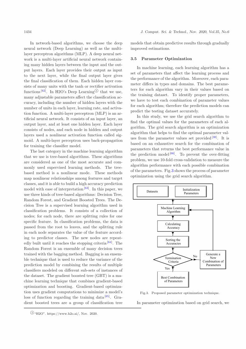
3.5 Parameter Optimization
In machine learning, each learning algorithm has a
set of parameters that affect the learning process and
the performance of the algorithm. Moreover, each para-
meter differs in types and domains. The best parame-
ters for each algorithm vary in their values based on
the training dataset. To identify proper parameters,
we have to test each combination of parameter values
for each algorithm; therefore the prediction models can
predict the testing dataset accurately.
In this study, we use the grid search algorithm to
find the optimal values for the parameters of each al-
gorithm. The grid search algorithm is an optimization
algorithm that helps to find the optimal parameter val-
ues from the parameter values set provided [30]. It is
based on an exhaustive search for the combination of
parameters that returns the best performance value in
the prediction model [66]. To prevent the over-fitting
problem, we use 10-fold cross-validation to measure the
algorithm performance with each possible combination
of the parameters. Fig.3 shows the process of parameter
optimization using the grid search algorithm.
Machine Learning Algorithm
Termination Criteria
Datasets
Generate a New
Combination of Parameters
Sorting the Accuracies
Best Combination of Parameters
InitializationParameters
Calculating Accuracy
No
Yes
Fig.3. Proposed parameter optimization technique.
In parameter optimization based on grid search, we
4○“H2O”. https://www.h2o.ai/, Nov. 2020.

Mohammad Y. Mhawish et al.: Predicting Code Smells and Analysis of Predictions 1435
identify a set of values for each parameter. For nomi-
nal parameters, we assign the nominal values as shown
in Table 3. We discretize the numeric parameters by
setting the value range as well as a number of steps in
the range. The values that must be tested are assigned
within upper and lower bounds of the range based on
the specified number of steps that are assigned for each
parameter, as shown in Table 4.
Table 3. Tuning Algorithms’ Nominal Parameters
Model Parameter Parameter Option
Decision tree Criterion Gain ratio, informationgain, Gini index,accuracy
Deep learning Activation function Tanh, Rectifier
Table 4. Tuning Algorithms’ Numeric Parameters and Numberof Steps Assigned for Each Parameter
Model Parameter Start End Step
Value Value
Random Forest Number of trees 1 100.0 10
Maximal depth 1 100.0 10
Gradient Boosted Number of trees 1 200.0 10Trees
Maximal depth 1 100.0 10
Decision Tree Maximal depth 1 100.0 10
Deep Learning Learning rate 0 1.0 10
SVM C 0 2 000.0 10
Gamma 1 100.0 10
MLP Learning rate 0 1.0 5
Momentum rate 0 0.5 5
3.6 Validation Methodology
In this study, we conduct a series of experiments
and apply a validation scenario to evaluate each experi-
ment’s performance. First, we use the 10-fold cross-
validation during the training process. The 10-fold
cross-validation is used to evaluate machine learning
models by dividing the dataset into 10 parts with 10
times of repetition. In each repetition, one different
part from data is taken as a test dataset, and the other
parts are for training the mode. Then, we test the
trained models with unseen test dataset (20% split-
ted from the dataset before training). The unseen test
datasets are used to explain the models’ predictions and
avoid generalization errors.
3.6.1 Performance Measures
For measuring the effectiveness of each experiment,
we consider five performance parameters such as preci-
sion, recall, F -score, area under the ROC curve (AUC),
and accuracy.
Precision & Recall. The precision measures the per-
centage of the correctly detected code smells instances
by the machine learning mode. The recall measures
what code smells instances are actually being detected
by the machine learning mode. Precision (P) and recall
(R) are calculated using the following formula.
precision =TP
TP + FP,
recall = true positive rate (TPR) =TP
TP + FN.
• True positive (TP ) denotes the instances that the
model correctly predicts in the positive class.
• False positive (FP ) denotes the instances that the
model incorrectly predicts in the positive class.
• True negative (TN) denotes the instances that the
model correctly predicts in the negative class.
• False negative (FN) denotes the instances that
the model incorrectly predicts in the negative class.
F -score (F-measure) is the harmonic average of pre-
cision and recall, while the precision is the positive-
classified instances that are positive, and the recall is
the real-positive instances classified as positive. F -
measure is a way of having a single number by com-
bining the two other measures (precision and recall)
and is calculated using the following formula.
F -score = 2×precision× recall
precision+ recall.
Accuracy is one of the performance measures for
classification. It is the percentage of correctly classified
instances in the positive and negative classes calculated
as follows.
Accuracy(AC) =TP + TN
TP + TN + FP + FN.
Area Under the ROC Curve (AUC). AUC is one
of the common measures of model accuracy for classi-
fication models by computing the area under the re-
ceiver operating characteristic (ROC) curves. ROC
curves are a way to visualize the tradeoffs between true-
positive and false-positive rates in a classifier to analyze
and compare the performance of the classifier models
through visual analytics.
3.6.2 Prediction Models Explanation
The use of classification accuracy to report the pre-
diction model’s performance could not be enough, and
it does not give a much comprehensive view about the
model behavior and the capability to draw its conclu-
sion.

1436 J. Comput. Sci. & Technol., Nov. 2020, Vol.35, No.6
We calculate the model’s confidences for each
prediction, which gives machine learning model’s
behavior [67]. Moreover, we use a model interpretation
method called the LIME algorithm to provide more
understanding of how the model makes its decision
and which features influence the model to make its
decision [68]. The LIME algorithm calculates each fea-
ture’s importance by generating a set of data points
around each feature individually. Then it applies the
trained model and observes the impact of each data
point in the prediction output. The local importance
of each feature is the correlation between the feature
and its effects on the prediction. Finally, each fea-
ture’s global importance is calculated and provided as
output [29].
4 Experimental Results and Discussions
In this section, we introduce results and discussions
for the experiments conducted in our approach.
4.1 First Experiment: Code Smells Prediction
Models from Binary-Label Datasets
To answer RQ1, we test the machine learning algo-
rithms on two types of datasets ORI D and REFD D.
The performance of the prediction models for the four
code smells datasets is reported in Table 5 and Ta-
bles S1–S3 of the online resource 5○. Each model’s
performance is calculated using 10-fold cross-validation
during the training process with a 20% unseen test
dataset.
4.1.1 Data Class
Table 5 shows the performance result of Data Class
prediction in ORI D and REFD D datasets. The Ran-
dom Forest algorithm scores the best 10-fold cross-
validation accuracy of 99.71% and 99.70% in the ORI D
and the REFD D datasets, respectively, and it scores
100% accuracy in the unseen test dataset in REFD D.
For the rest of the models, there is no significant diffe-
rence in accuracy, where the accuracy ranges from 95%
in MLP to 98% in GBT. By computing the confidence
level for each prediction, we find that the Random For-
est model is most likely to predict more non-smelly in-
stances as compared with Data Class instances with
confidence level of 100% in the ORI D dataset and
around 70% in the REFD D dataset. Hence, despite
the high accuracy of the model, it is not reliable be-
cause of the high divergence in the confidence level in
the ORI D dataset.
Using the LIME algorithm, the metrics that sup-
port the Random Forest model’s decision for predicting
smelly instances are the number of accessor methods
(NOAM), the weight of class (WOC), and response for
a class (RFC). On the other hand, the metrics that sup-
port the model’s decision for predicting the non-smelly
instances are weighted methods count of not accessor
or mutator methods (WMCNAMM), called foreign not
accessor or mutator methods (CFNAMM), and lines
of code without accessor or mutator methods (LOC-
NAMM).
Table 5. Data Class: Evaluation Results for ORI D and REFD D Datasets
Dataset Model Cross-Validation Validation Test
Accuracy (%) AUC (%) F -Score (%) R (%) P (%) Accuracy (%) R (%) P (%)
ORI D Deep learning 96.47 99.70 97.14 94.64 100.00 97.62 98.21 98.21
Decision tree 97.34 89.70 98.02 98.68 97.50 98.81 98.21 100.00
GBT 98.51 99.90 98.88 98.22 99.58 100.00 100.00 100.00
SVM 97.06 99.20 97.80 98.22 97.58 94.05 94.64 96.36
Random forest 99.71 100.00 99.79 100.00 99.58 97.62 100.00 96.55
MLP 95.87 96.60 96.90 97.33 96.69 95.24 98.21 94.83
REFD D Deep learning 97.23 98.90 97.87 97.66 98.13 96.34 98.15 96.36
Decision tree 97.85 74.40 98.34 97.68 99.07 98.78 100.00 98.18
GBT 98.79 100.00 99.06 98.18 100.00 97.56 96.30 100.00
SVM 96.01 99.00 96.96 96.75 97.21 95.12 96.30 96.30
Random forest 99.70 100.00 99.78 100.00 99.57 100.00 100.00 100.00
MLP 95.41 96.00 96.56 98.14 95.15 96.34 98.15 96.36
5○The online resource mentioned in this paper is available at: https://doi.org/10.6084/m9.figshare.13078547, Oct. 2020.

Mohammad Y. Mhawish et al.: Predicting Code Smells and Analysis of Predictions 1437
4.1.2 God Class
In Table S1 of the online resource 6○, we present the
performance result of God Class prediction in ORI D
and REFD D datasets. The Gradient Boosted Trees
(GBT) and Random Forest algorithms have shown the
best score of 10-fold cross-validation values of 98.48%
in the REFD D dataset, and 97.61%, 97.60% in the
ORI D dataset. The Random Forest algorithm has
recorded the best F -score and AUC values of 98.84%
and 99.70% in the REFD D dataset respectively. In
the unseen test dataset, the Random Forest algorithm
scores the accuracy of 93.90% in the REFD D dataset
and 98.81% in the ORI D dataset.
The confidence level of predicting God Class in
ORI D and REFD D datasets is 92%, 77% for the GBT
model respectively, and 97%, 94% for the Random For-
est model respectively. The software metrics that sup-
port the Random Forest model’s decision to predict
God Class prediction are the weighted methods count of
not accessor or mutator methods (WMCNAMM), lines
of code without accessor or mutator methods (LOC-
NAMM), lines of code (LOC), weighted methods count
(WMC), and the number of called classes (FANOUT).
4.1.3 Long Method
The best algorithm for predicting Long Method
smells is the Random Forest algorithm with an accu-
racy of 99.71% and 95.97% in the ORI D and REFD D
datasets as shown in Table S2 of the online resource 6○.
The highest AUC value of 100% was recorded for GBT
and Random Forest algorithms in the ORI D dataset.
The Random Forest also scores the best F -score value
in ORI D and REFD D datasets of 99.78% and 96.61%
respectively. In the unseen test dataset, the Random
Forest algorithm in the ORI D dataset scores 100% ac-
curacy with 100% precision. Whereas, GBT and Deci-
sion Tree algorithms score the best accuracy of 89.19%
in the unseen test dataset in REFD D.
In the REFD D dataset, all of the models have
a higher confidence level to predict Long Method in-
stances than non-smelly instances. The GBT model
scores the highest confidence level of 94% in the
REFD D dataset. While in the ORI D dataset, the
Random Forest model is likely to predict more non-
smelly instances as compared with Long Method in-
stances with a confidence level of 57%. The essential
metrics that support the GBT model’s decision are the
number of code lines in the method (LOC-method), cy-
clomatic complexity (CYCLO), the number of methods
overridden (NMO) in the class, access to local data
(ATLD), the number of local variables (NOLV), and
lines of code in the package (LOC-package).
4.1.4 Feature Envy
As shown in Table S3 of the online resource 6○,
the Random Forest and Decision Tree algorithms
achieve the highest accuracies of 97.64%, 97.97% in the
REFD D dataset respectively, and 97.34%, 97.03% in
the ORI D dataset respectively. Moreover, the Ran-
dom Forest algorithm scores the best F -score values of
98.12%, 97.96%, and the best AUC values of 99% in
the ORI D and REFD D datasets. In the unseen test
dataset, the Random Forest and Decision Tree algo-
rithms score the best accuracies of 97.62% in the ORI D
dataset and 95.95% in the REFD D dataset.
The Decision Tree model scores the highest confi-
dence level of predicting Feature Envy by 98% in the
REFD D dataset. The software metrics that support
this decision are access to foreign data (ATFD) and
coupling dispersion (CDISP).
4.1.5 Discussion About Software Metrics and Their
Effectiveness in Code Smell Prediction
From the results reported in Table 5 and Tables S1–
S3 of the online resource 6○, we observe that the best
algorithms for predicting code smells are tree-based al-
gorithms. The prediction process in these algorithms is
done by the prediction rules consisting of metrics and
thresholds for these metrics. We extract the prediction
rules generated by the Decision Tree algorithm in order
to study the effectiveness of using software metrics to
predict code smells.
Based on these rules, the model predicts the most
Data Class instances under the following conditions.
WOC type 6 0.356 &&
NOAM type >
2.500 && RFC type 6 43
Most of the Data Class instances are detected if the
weight of the class (WOC) is less than or equal to 0.356,
the class has more than two accessor methods, and the
value of the response (RFC) for the class is less than
43. These metrics measure several quality dimensions
of software. NOAM measures the coupling, RFC mea-
sures the complexity, and WOC measures the size.
In the God Class dataset, the prediction rules to
predict God Class instances are as follows.
6○The online resource mentioned in this paper is available at: https://doi.org/10.6084/m9.figshare.13078547, Oct. 2020.

1438 J. Comput. Sci. & Technol., Nov. 2020, Vol.35, No.6
WMCNAMM > 47.50
Or
WMCNAMM 6 47.50 && LOCNAMM >415
The most God Class instances are being detected if
weighted methods count of not accessor or mutator
methods (WMCNAMM) is greater than 47.50. The re-
maining instances are detected when the WMCNAMM
value is less than or equal to 47.50 and lines of code
without accessor or mutator methods (LOCNAMM) is
higher than 415, where WMCNAMM and LOCNAMM
measure the complexity and the size of the software.
In the Long Method dataset, the prediction rules to
predict Long Method instances are as follows.
LOC method > 79.50 && CYCLO method >7.50
Based on these conditions, the model detects the
Long Method smells if the number of code lines (LOC)
of the method is greater than 79.50, and the cyclo-
matic complexity (CYCLO) of the method is greater
than 7.50, where both of these metrics measure the size
of the software.
In the Feature Envy, the prediction rules to predict
Feature Envy instances are as follows.
ATFD method > 4.50 && LAA method 6 0.323
The rules state that most of the Long Method in-
stances are detected when the value of access to for-
eign data (ATFD) is greater than 4.50. The remaining
false-positive instances are filtered through the second
rule when the value of the locality of attribute accesses
(LAA) is less than or equal to 0.323, where ATFD and
LAA measure the complexity and encapsulation of the
software.
Table 6 shows a comparison of our approach with
other related work. These approaches applied ma-
chine learning to the binary-label dataset proposed by
Fontana et al. [24] In the Data Class dataset, our ap-
proach scores the best accuracy of 99.70% and F -score
of 99.78% using the Random Forest algorithm while
the Fontana et al.’s approach [24] scores 99.02% accu-
racy and 99.26% F -score using the B-J48 Pruned al-
gorithm. Likewise, in the God Class dataset, our ap-
proach scores the best accuracy of 98.48% and F -score
of 98.83% using the GBT algorithm while Fontana et
al.’s approach [24] scores 97.55% accuracy and 98.14%
F -score using the Naıve Bayes algorithm. In the Long
Method dataset, Fontana et al.’s approach [24] scores
the best accuracy of 99.43% and 99.49% F -scored us-
ing the B-J48 Pruned algorithm. In contrast, Guggu-
lothu and Moiz’s approach [69] scores 95.9% accuracy
and 96% F -score while our approach scores 95.97% ac-
curacy and 96.61% F -score using the Random Forest
algorithm. In the Feature Envy dataset, our approach
scores 97.97% accuracy and 98.39% F -score using the
Decision Tree algorithm. In comparison, Fontana et
al.’s approach [24] scores 96.64% accuracy and 97.44%
F -score using the B-JRip algorithm, while Guggulothu
and Moiz’s approach [69] scores the best accuracy of
99.1% and 99% F -score using the B-J48 Pruned algo-
rithm.
4.2 Second Experiment: Code Smell
Prediction Models from Multi-Label
Datasets
To answer RQ2, we apply a multi-label prediction
on the MULTI L D dataset. Tables 7 and 8 show the
performance results of six machine learning algorithms
for predicting code smells in multi-label datasets.
In the Class-Level dataset, the Random Forest al-
gorithm scores the highest cross-validation accuracy
of 97.11% with 97.22% weighted mean precision (P),
and 97.31% weighted mean recall (R). By measuring
each prediction’s confidence level in the Random Forest
model, the results indicate that the model has the high-
est confidence level to predict the God Class of 91%.
The most critical metrics that support the Random
Forest decision are weighted methods count (WMC),
weighted methods count of not accessor or mutator
methods (WMCNAMM), average methods weight of
not accessor or mutator methods (AMWNAMM), lines
of code without accessor or mutator methods (LOC-
NAMM), and response for a class (RFC).
Table 6. Comparison Among Our Approach with Other Related Work (Binary-Label Dataset)
Code Smells Fontana et al. [24] Guggulothu & Moiz [69] Our ApproachDataset
Best Accuracy F -Score Best Accuracy F -Score Best Accuracy F -Score
Algorithm (%) (%) Algorithm (%) (%) Algorithm (%) (%)
Data Class B-J48 Pruned 99.02 99.26 N/A N/A Random Forest 99.70 99.78
God Class Naıve Bayes 97.55 98.14 N/A N/A GBT 98.48 98.83
Long Method B-J48 Pruned 99.43 99.49 Random Forest 95.90 96 Random Forest 95.97 96.61
Feature Envy B-JRip 96.64 97.44 B-J48 Pruned 99.10 99 Decision Tree 97.97 98.39

Mohammad Y. Mhawish et al.: Predicting Code Smells and Analysis of Predictions 1439
Table 7. Evaluation Results for the Class-Level Dataset
Model Accuracy (%) God Class Data Class No-Smell
R (%) P (%) R (%) P (%) R (%) P (%)
Deep Learning 91.75 97.14 88.89 95.71 93.06 83.83 93.33Decision Tree 95.97 96.43 94.41 99.29 96.53 92.81 96.88GBT 96.20 97.14 95.10 100.00 95.89 92.22 97.47SVM 93.10 91.43 96.24 92.86 97.01 94.61 87.78Random Forest 97.11 98.57 95.83 99.29 97.20 94.01 98.12MLP 92.19 94.29 92.96 92.14 94.85 90.42 89.35
Table 8. Evaluation Results for the Method-Level Dataset
Model Accuracy (%) Feature Envy Long Method No-Smell
R (%) P (%) R (%) P (%) R (%) P (%)
Deep Learning 94.15 98.18 93.10 83.64 92.00 96.58 95.27Decision Tree 96.11 98.18 96.43 96.36 88.33 95.21 99.29GBT 96.12 98.18 93.10 94.55 89.66 95.89 100.00SVM 93.34 90.91 96.15 90.91 84.75 95.21 95.86Random Forest 96.91 98.18 96.43 100.00 90.16 95.21 100.00MLP 92.94 89.09 94.23 96.36 91.38 93.33 93.33
As shown in Table 7, the Random Forest scores the
best recall value of 98.57% and 99.29% in predicting
the God Class instance, and the Data Class instances
respectively. The model predicts most of the smelly in-
stances with high recall value despite the little low pre-
cision value, due to the false positives from non-smelly
instances.
Through the interpretations of the prediction rules
in the Decision Tree model, we find that the main met-
rics that support the model to predict God Class are
weighted methods count (WMC), and called foreign not
accessor or mutator methods (CFNAMM). The model
predicts the most God Class instances in the dataset
when WMC > 43.5, while the model distinguishes be-
tween God Class instances and non-smelly instances
with high recall and precision when CFNAMM > 2.5.
On the other side, the main metrics that support the
model to predict Data Class instances are the number
of accessor methods (NOAM) and the number of in-
herited methods (NIM). The model predicts the most
Data Class instances in the dataset when WMC 6 43.5
& NOAM > 2.5 & NIM 6 26.977. Fig.4 shows the
entire prediction rules for the Class-Level dataset.
Table 8 shows models performance in the Method-
Level dataset. The Random Forest model scores the
highest accuracy of 96.91%. The recall values in this
model to predict Feature Envy and Long Method smells
are 98.18% and 100% respectively. The model has the
confidence of 55% and 42% to predict Long Method and
Feature Envy smells respectively. The essential metrics
that support the model’s decision to predict the Long
Method are cyclomatic complexity (CYCLO) and the
locality of attribute accesses (LAA). Besides, the met-
ric that supports the model decision to predict Feature
Envy is access to foreign data (ATFD).
In the Decision Tree model, the prediction rules
show that the main metrics that support the model to
predict Long Method instances are ATFD and CYCLO.
Most of the Long Method instances are detected when
ATFD 6 4.500 and CYCLO > 7.500. The critical met-
rics that support the model to predict Feature Envy are
LAA and ATFD. The model detects the most Feature
Envy instances in the dataset when LAA 6 0.560 and
ATFD > 4.500. Fig.5 shows the entire prediction rules
for the Method-Level dataset.
Table 9 presents a comparison between our ap-
proach and other related approaches in the multi-label
dataset. As presented in the table, our approach
achieves the best accuracy of 97.11% and 96.91% when
using the Random Forest algorithm in the Class-Level
and Method-Level datasets respectively. In the ap-
proach proposed by Kiyak et al. [70], the Random Forest
algorithm scores the best accuracy of 96.9% and 93.6%
in the Class-Level and Method-Level datasets. In Gug-
gulothu and Moiz’s approach [69], the Random Forest
scores the best accuracy of 93.5% in the Method-Level
dataset.
4.3 Third Experiment: Impact of Feature
Selection Methods on Code Smell
Prediction Models
This experiment aims to investigate the influence
of the feature selection techniques on enhancing the
model accuracy and recognizing the software metrics

1440 J. Comput. Sci. & Technol., Nov. 2020, Vol.35, No.6
WMC
> 43.5 43.5
2.5> 2.5
2.5> 2.5
> 26.9
26.9
CFNAMM NOAM
God Class
Data Class
Result:God Class = 111Data Class = 0
No-Smell = 2
Result:God Class = 1Data Class = 0
No-Smell = 6
Result:God Class = 0Data Class = 0
No-Smell = 93
Result:God Class = 1Data Class = 0
No-Smell = 7
Result:God Class = 0
Data Class = 11
No-Smell = 2
No-Smell
No-Smell
No-SmellNIM
<-
< <- -
<-
Fig.4. Prediction rules (class-level dataset).
0.56
> 4.5
> 0.56 > 7.5
ATFD
LAA CYCLO
Result:Feature Envy = 0Long Method = 3
No-Smell = 0
Result:Feature Envy = 55Long Method = 1
No-Smell = 2
Result:Feature Envy = 0Long Method = 51
No-Smell = 5
Result:Feature Envy = 0Long Method = 0No-Smell = 139
4.5
7.5
Long Method Feature Envy Long Method No-Smell
<- <-
<-
Fig.5. Prediction rules (method-level dataset).
Table 9. Comparison of Our Approach and Other Related Works (Multi-Label Dataset)
Code Smells Kiyak et al. [70] Guggulothu & Moiz [69] Our Approach
DatasetBest Algorithm Accuracy (%) Best Algorithm Accuracy (%) Best Algorithm Accuracy (%)
Method-Level Random Forest 93.6 Random Forest 93.5 Random Forest 96.91
Class-Level Random Forest 96.9 N/A N/A Random Forest 97.11
that play a substantial role in the code smells prediction
process. To answer RQ3, we use two feature selection
methods based on the Genetic algorithm. In Tables S4
and S5 of the online resource 7○, we present the selected
sets of features that are created by feature selection
methods for binary-label and multi-label datasets. The
7○The online resource mentioned in this paper is available at: https://doi.org/10.6084/m9.figshare.13078547, Oct. 2020.

Mohammad Y. Mhawish et al.: Predicting Code Smells and Analysis of Predictions 1441
GA-Naıve Bayes and GA-CFS methods select nine and
seven metrics in Data Class and God Class respec-
tively, 11 and seven metrics in Feature Envy respec-
tively, and both eight metrics in LongMethod, as shown
in Table S4 of the online resource 8○. In the Class-
Level dataset, the GA-Naıve Bayes method selects 13
metrics while the GA-CFS selects 17 metrics. In the
Method-Level dataset, the GA-Naıve Bayes method se-
lects 12 metrics, while the GA-CFS selects five metrics,
as shown in Table S5 of the online resource 8○.
In Tables 10 and 11, we compare the percentage ac-
curacy of all algorithms before and after applying fea-
ture selection method. In general, a slight enhancement
occurs in most of the models. The GA-CFS method
is the most efficient in enhancing accuracy. The re-
sults indicate that using all-features yield better perfor-
mance in some cases of the Random Forest and GBT
algorithms. On the other hand, the feature selection
methods significantly enhance accuracies in some mod-
els such as Decision Tree, SVM, and Deep Learning
model.
4.4 Fourth Experiment: Impact of Tuning
Machine Learning Parameters on Code
Smell Prediction Models
To answer RQ4, we look at the influence of tuning
the machine learning algorithm’s parameters on perfor-
mance. The six different combinations of parameters
for each algorithm are presented in Tables 12–14 and
Tables S6-S8 of the online resource 8○.
In the Random Forest model, the best accuracy of
99.70% is achieved when the number of trees is 31, and
the maximal depth is 21. Table 12 shows that when
the number of trees grows and the maximal depth re-
mains constant, the accuracy decreases. In the GBT
model, the best accuracy is recorded as 98.48% when
the number of trees and the maximal depth is 12.
When the maximal depth is reduced to 2, the accuracy
is decreased to 97.87%. In the Decision Tree model,
the best accuracy of 95.61% is scored when the crite-
rion is a gain ratio, and the maximal depth is 9. As
observed, when the criterion is changed to “accuracy”
Table 10. Effect of Feature Selection Methods on Prediction Models for the Binary-Label Dataset
Code Smells Model GA-Naıve Bayes GA-CFS ALL Features
DatasetAccuracy (%) F -Score (%) Accuracy (%) F -Score (%) Accuracy (%) F -Score (%)
Data Class Deep Learning 96.94 97.70 97.24 97.93 97.23 97.87
Decision Tree 96.03 97.00 98.16 98.57 97.85 98.34
GBT 97.86 98.36 98.17 98.59 98.79 99.06
SVM 97.55 98.17 98.17 98.59 96.01 96.96
Random Forest 98.48 98.85 99.39 99.55 99.70 99.78
MLP 92.67 94.38 86.60 89.12 95.41 96.56
God Class Deep Learning 98.79 99.08 98.17 98.62 98.17 98.57
Decision Tree 97.57 98.14 98.47 98.83 97.86 98.37
GBT 98.18 98.63 98.48 98.83 98.48 98.83
SVM 98.48 98.86 97.88 98.42 97.88 98.42
Random Forest 98.18 98.62 98.48 98.85 98.48 98.84
MLP 98.17 98.64 86.60 89.12 97.26 97.98
Long Method Deep Learning 94.59 95.56 95.29 96.04 93.26 94.23
Decision Tree 94.24 95.08 94.28 95.25 95.61 96.34
GBT 94.57 95.43 95.97 96.66 95.61 96.90
SVM 94.57 95.56 94.61 95.54 90.86 92.61
Random Forest 94.93 95.71 95.95 96.63 95.97 96.61
MLP 93.60 94.77 97.88 98.42 92.55 93.88
Feature Envy Deep Learning 97.97 98.43 98.32 98.67 94.93 95.70
Decision Tree 97.97 98.39 96.64 97.34 97.97 98.39
GBT 96.97 97.58 97.30 97.85 97.63 98.13
SVM 97.63 98.12 97.31 97.89 96.30 97.02
Random Forest 97.97 98.40 97.98 98.39 97.64 98.12
MLP 96.29 97.15 95.63 96.69 92.92 94.30
8○The online resource mentioned in this paper is available at: https://doi.org/10.6084/m9.figshare.13078547, Oct. 2020.

1442 J. Comput. Sci. & Technol., Nov. 2020, Vol.35, No.6
Table 11. Effect of Feature Selection Methods on PredictionModels for the Multi-Label Dataset
Code Smells Model Accuracy (%)
Dataset GA-Naıve GA-CFS All
Bayes Features
Class-Level Deep Learning 91.30 92.86 91.75
Decision Tree 94.64 96.42 95.97
GBT 95.31 96.20 96.20
SVM 92.20 93.08 93.10
Random Forest 95.31 96.88 97.11
MLP 92.20 91.09 92.19
Method-Level Deep Learning 94.15 94.17 94.15
Decision Tree 96.11 96.11 96.11
GBT 96.12 95.71 96.12
SVM 93.34 94.57 93.34
Random Forest 96.91 96.11 96.91
MLP 92.94 93.38 92.94
Table 12. Effect of Parameter Optimization Technique on theAccuracy of the Random Forest Model
Number of Trees Maximal Depth Accuracy (%)
31 21 99.70
41 21 99.09
100 21 98.78
11 31 98.16
1 21 94.80
1 80 91.77
Table 13. Effect of Parameter Optimization Technique on theAccuracy of the Gradient Boosted Trees Model
Number of Trees Maximal Depth Accuracy (%)
12 12 98.48
5 2 98.17
7 2 97.87
3 31 97.57
12 2 97.87
14 2 97.87
Table 14. Effect of Parameter Optimization Technique on theAccuracy of the Decision Tree Model
Maximal Depth Criterion Accuracy (%)
9 Gain ratio 95.61
9 Accuracy 94.28
9 Gini index 93.59
9 Information gain 91.86
100 Gini index 93.59
100 Information gain 91.86
or “Gini index” or “information gain” with a fixed num-
ber of maximal depths, the accuracy of the model de-
creases. In the SVMmodel, the best accuracy of 97.63%
is scored when the value of parameter C is 1 800 and
gamma is zero. It is observed that when the value of
C is 1 800, the accuracy decreases gradually as gamma
increases. In the Multilayer Perceptron model, the best
combination of parameters that score the best accuracy
is 0.45 for Learning Rate and 0.5 for Momentum Rate.
In the same case, when the Momentum Rate is set to
0, the accuracy is decreased from ∼97% to ∼94%. The
Deep Learning model achieves the best accuracy when
the learning rate equals 1, and the activation function
is the rectifier. In the same case, when the learning
rate equals 1 and the activation function is tanh, the
accuracy is decreased from 98.32% to 96.97%. When
the activation function is the rectifier, and the learning
rate value is 0.9, the accuracy decreases to 96.62%.
From the results, we observe that the parameter op-
timization technique positively effects on enhancing the
accuracy of the machine learning algorithms.
5 Threats to Validity
In this section, we discuss the possible threats that
might have affected our approach and how we mitigate
them.
5.1 Threats to Internal Validity
The main threat to internal validity is datasets. The
datasets used in our approach are constructed from
datasets published by Fontana et al. [24] According to
the study published by Di Nucci et al. [71], the reference
datasets are unreliable datasets that show a lack in the
real distribution of code smells and imbalanced metrics
distributions.
We manage this threat by modifying the original
datasets in order to increase the realism of the data
in terms of smells actual presence in the software sys-
tem. The distribution of the dataset is modified by
mixing instances of other smells with non-smelly in-
stances. Moreover, we remove the non-smelly instances
with a classification confidence value that is higher than
95% to ensure a more smoothed boundary between the
metrics distributions, as described in Subsection 3.1.
5.2 Threats to Conclusion Validity
This threat centers on evaluating the performance of
the prediction models. We use 10-fold cross-validation
in order to evaluate the predictive models by using
many evaluation metrics, including accuracy, AUC, F -
measure, precision, and recall. These evaluation met-
rics may not be enough to evaluate the predictive model
and may not have the ability to predict smelly instances

Mohammad Y. Mhawish et al.: Predicting Code Smells and Analysis of Predictions 1443
due to many reasons, including the result of the ma-
chine learning models being a black box.
We manage this threat by calculating the confidence
value for each prediction and extracting the metrics
that support the prediction model to take its decision.
This explanation provides more information about the
model behavior in the prediction and shows the factors
that affect the results.
5.3 Threats to External Validity
The threats to external validity are summarized as
follows. First, the number of code smells used in our
experiments is limited to only two class-level and two
method-level smells. Second, our findings may not be
enough to generalize to all software in the industrial
domain.
6 Conclusions
In this paper, we proposed an approach based on
machine learning and software metrics to detect code
smells from software systems and found the metrics that
play critical roles in the detection process. Two types
of datasets were created by using the dataset published
by Fontana et al. [24] The Genetic algorithm is applied
for feature selection methods, and it is observed that
the accuracy of all algorithms can be enhanced by se-
lecting the most relevant features in each dataset. The
Grid search algorithm used in the parameter optimiza-
tion technique significantly enhanced the accuracy of
all algorithms.
We conducted a set of experiments using six
machine learning algorithms. In the Binary-Label
datasets, the tree-based algorithms achieve the best ac-
curacy values. The Random Forest tree model achieves
the best accuracy of 99.71% and 99.70% in predicting
the Data Class in the ORI D and REFD D datasets
respectively. The GBT algorithm achieves 97.60% and
98.48% to predict the God Class in the ORI D and
REFD D datasets respectively. In the Long Method,
the Random Forest algorithm scores the accuracy of
99.71% and 95.97% in the ORI D and the REFD D
datasets respectively. The Decision Tree algorithm
achieves the accuracy of 97.03% and 97.97% in the
Feature Envy code smells in the ORI D and REFD D
datasets respectively.
We also conducted a set of experiments using multi-
label datasets. In the Class-Level dataset, the tree-
based models achieve the best performance results with
the accuracy of 97.11%, 96.20%, and 95.97% by Ran-
dom Forest, GBT, and Decision Tree algorithms respec-
tively. The Random Forest algorithm achieves the best
recall and precision of 98.57% and 95.83% for predicting
God Class respectively. Further, the best recall and the
precision to predict Data Class are 99.29% and 97.20%
respectively. In the Method-Level dataset, the tree-
based models achieve the best performance of 96.91%,
96.12%, and 96.11% by Random Forest, GBT, and De-
cision Tree algorithms respectively. The Random For-
est algorithm scores the best recall and the precision
of 100% and 90.16% for the Long Method smell respec-
tively. In addition, the Random Forest algorithm scores
the best recall and precision of 98.18% and 96.43% for
Feature Envy smells respectively.
Finally, the machine learning techniques showed
high potential in predicting the code smells that en-
hance the quality of software.
References
[1] Wiegers K, Beatty J. Software Reqirements. Pearson Edu-
cation, 2013.
[2] Chung L, do Prado Leite J C S. On non-functional re-
quirements in software engineering. In Conceptual Mod-
eling: Foundations and Applications-Essays in Honor of
John Mylopoulos, Borgida AT, Chaudhri V, Giorgini P, Yu
E (eds.), Springer, 2009, pp.363-379.
[3] Fowler M, Beck K, Brant J, Opdyke W, Roberts D. Refac-
toring: Improving the Design of Existing Code (1st edition).
Addison-Wesley Professional, 1999.
[4] Yamashita A, Moonen L. Exploring the impact of inter-
smell relations on software maintainability: An empirical
study. In Proc. the 35th Int. Conf. Softw. Eng., May 2013,
pp.682-691.
[5] Yamashita A, Counsell S. Code smells as system-level in-
dicators of maintainability: An empirical study. J. Syst.
Softw., 2013, 86(10): 2639-2653.
[6] Yamashita A, Moonen L. Do code smells reflect important
maintainability aspects? In Proc. the 28th IEEE Int. Conf.
Softw. Maintenance, September 2012, pp.306-315.
[7] Sjøberg D I K, Yamashita A, Anda B C D, Mockus A, Dyba
T. Quantifying the effect of code smells on maintenance ef-
fort. IEEE Trans. Softw. Eng., 2013, 39(8): 1144-1156.
[8] Sahin D, Kessentini M, Bechikh S, Ded K. Code-smells
detection as a bi-level problem. ACM Trans. Softw. Eng.
Methodol., 2014, 24(1): Article No. 6.
[9] Olbrich S, Cruzes D S, Basili V, Zazworka N. The evolu-
tion and impact of code smells: A case study of two open
source systems. In Proc. the 3rd International Symposium
on Empirical Software Engineering and Measurement, Oc-
tober 2009, pp.390-400.
[10] Olbrich S M, Cruzes D S, Sjoøberg D I K. Are all code smells
harmful? A study of God Classes and Brain Classes in the
evolution of three open source systems. In Proc. the 26th
IEEE Int. Conf. Softw. Maintenance, September 2010.

1444 J. Comput. Sci. & Technol., Nov. 2020, Vol.35, No.6
[11] Khomh F, Penta D M, Gueheneuc Y G. An exploratory
study of the impact of code smells on software change-
proneness. In Proc. the 16th Working Conference on Re-
verse Engineering, October 2009, pp.75-84.
[12] Deligiannis I, Stamelos I, Angelis L, Roumeliotis M, Shep-
perd M. A controlled experiment investigation of an object-
oriented design heuristic for maintainability. J. Syst. Softw.,
2004, 72(2): 129-143.
[13] Perez-Castillo R, Piattini M. Analyzing the harmful ef-
fect of god class refactoring on power consumption. IEEE
Softw., 2014, 31(3): 48-54.
[14] Li W, Shatnawi R. An empirical study of the bad smells and
class error probability in the post-release object-oriented
system evolution. J. Syst. Softw., 2007, 80(7): 1120-1128.
[15] Ciupke O. Automatic detection of design problems in
object-oriented reengineering. In Proc. the 30th Interna-
tional Conference on Technology of Object-Oriented Lan-
guages and Systems, Delivering Quality Software, August
1999, pp.18-32.
[16] Travassos G, Shull F, Fredericks M, Basili V R. Detecting
defects in object-oriented designs: Using reading techniques
to increase software quality. ACM SIGPLAN Notices, 1999,
34(10): 47-56.
[17] Dashofy E M, van der Hoek A, Taylor R N. A comprehen-
sive approach for the development of modular software ar-
chitecture description languages. ACM Trans. Softw. Eng.
Methodol., 2005, 14(2): 199-245.
[18] Vidal S, Vazquez H, Dıaz-Pace J A, Marcos C, Garcia A,
Oizumi W. JSpIRIT: A flexible tool for the analysis of code
smells. In Proc. the 34th Int. Conf. Chil. Comput. Sci. Soc.,
November 2016.
[19] Marinescu R. Measurement and quality in object-oriented
design. In Proc. the 21st IEEE Int. Conf. Softw. Mainte-
nance, September 2005, pp.701-704.
[20] Moha N, Gueheneuc Y, Duchien L, le Meur A. DECOR:
A method for the specification and detection of code and
design smells. IEEE Trans. Softw. Eng., 2010, 36(1): 20-36.
[21] Fontana F A, Zanoni M, Marino A, Mantyla M V. Code
smell detection: Towards a machine learning-based ap-
proach. In Proc. the 2013 IEEE Int. Conf. Softw. Main-
tenance, September 2013, pp.396-399.
[22] Azadi U, Fontana F A, Zanoni M. Machine learning based
code smell detection through WekaNose. In Proc. the 40th
Int. Conf. Softw. Eng., May 2018, pp.288-289.
[23] Fontana F A, Zanoni M. Code smell severity classification
using machine learning techniques. Knowledge-Based Syst.,
2017, 128: 43-58.
[24] Fontana F A, Mantyla M V, Zanoni M, Marino A. Compar-
ing and experimenting machine learning techniques for code
smell detection. Empir. Softw. Eng., 2016, 21(3): 1143-
1191.
[25] Sharma T, Spinellis D. A survey on software smells. J. Syst.
Softw., 2018, 138: 158-173.
[26] Rasool G, Arshad Z. A review of code smell mining tech-
niques. J. Softw. Evol. Process, 2015, 27(11): 867-895.
[27] Fernandes E, Oliveira J, Vale G, Paiva T, Figueiredo E.
A review-based comparative study of bad smell detec-
tion tools. In Proc. the 20th International Conference on
Evaluation and Assessment in Software Engineering, June
2016, Article No. 18.
[28] Fontana F A, Braione P, Zanoni M. Automatic detection of
bad smells in code: An experimental assessment. J. Object
Technol., 2012, 11(2): Article No. 5.
[29] Riberro M T, Singh S, Guestrin C. “Why should I
trust you?”: Explaining the predictions of and classifier.
https//arxiv.org/abs/1602.04938, Oct. 2020.
[30] Chicco D. Ten quick tips for machine learning in computa-
tional biology. BioData Mining, 2017, 10(1): 35.
[31] Marinescu R. Detection strategies: Metrics-based rules
for detecting design flaws. In Proc. the 20th IEEE Inter-
national Conference on Software Maintenance, December
2004, pp.350-359.
[32] Abılio R, Padilha J, Figueiredo E, Costa H. Detecting code
smells in software product lines — An exploratory study.
In Proc. the 12th International Conference on Information
Technology-New Generations, April 2015, pp.433-438.
[33] Fenske W, Schulze S. Code smells revisited: A variability
perspective. In Proc. the 9th International Workshop on
Variability Modelling of Software-Intensive Systems, Jan-
uary 2015, Article No. 3.
[34] Suryanarayana G, Samarthyam G, Sharma T. Refactoring
for Software Design Smells: Managing Technical Debt (1st
edition). Morgan Kaufmann, 2014.
[35] Baudry B, Traon Y L, Sunye G, Jezequel J M. Measuring
and improving design patterns testability. In Proc. the 9th
IEEE International Software Metrics Symposium, Septem-
ber 2003.
[36] Langelier G, Sahraoui H, Poulin P. Visualization-based ana-
lysis of quality for large-scale software systems. In Proc. the
20th IEEE/ACM International Conference on Automated
Software Engineering, November 2005, pp.214-223.
[37] Murphy-Hill E, Black A P. An interactive ambient visuali-
zation for code smells. In Proc. the 5th International Sym-
posium on Software Visualization, October 2010, pp.5-14.
[38] de Figueiredo Carneiro G, Silva M, Mara L et al. Identifying
code smells with multiple concern views. In Proc. the 24th
Brazilian Symposium on Software Engineering, September
2010, pp.128-137.
[39] Kreimer J. Adaptive detection of design flaws. Electron.
Notes Theor. Comput. Sci., 2005, 141(4): 117-136.
[40] Amorim L, Costa E, Antunes N, Fonseca B, Ribeiro M.
Experience report: Evaluating the effectiveness of decision
trees for detecting code smells. In Proc. the 26th IEEE In-
ternational Symposium on Software Reliability Engineer-
ing, November 2015, pp.261-269.
[41] Khomh F, Vaucher S, Gueheneuc Y G, Sahraoui H. A
Bayesian approach for the detection of code and design
smells. In Proc. the 9th International Conference on Qua-
lity Software, August 2009, pp.305-314.
[42] Khomh F, Vaucher S, Gueheneuc Y G, Sahraoui H. BD-
TEX: A GQM-based Bayesian approach for the detection
of antipatterns. J. Syst. Softw., 2011, 84(4): 559-572.
[43] Vaucher S, Khomh F, Moha N, Gueheneuc Y G. Tracking
design smells: Lessons from a study of god classes. In Proc.
the 16th Working Conference on Reverse Engineering, Oc-
tober 2009, pp.145-154.
[44] Hassaine S, Khomh F, Gueheneuc Y G, Hamel S. IDS: An
immune-inspired approach for the detection of software de-
sign smells. In Proc. the 7th International Conference on
the Quality of Information and Communications Techno-
logy, September 2010, pp.343-348.

Mohammad Y. Mhawish et al.: Predicting Code Smells and Analysis of Predictions 1445
[45] Maiga A, Ali N, Bhattacharya N et al. Support vec-
tor machines for anti-pattern detection. In Proc. the 27th
IEEE/ACM International Conference on Automated Soft-
ware Engineering, September 2012, pp.278-281.
[46] Maiga A, Ali N, Bhattacharya N, Sabane A, Gueheneuc
Y G, Aimeur E. SMURF: A SVM-based incremental anti-
pattern detection approach. In Proc. the 19th Working
Conference on Reverse Engineering, October 2012, pp.466-
475.
[47] Tempero E, Anslow C, Dietrich J et al. The Qualitas Cor-
pus: A curated collection of Java code for empirical studies.
In Proc. the 17th Asia Pacific Software Engineering Confe-
rence, November 2010, pp.336-345.
[48] Pecorelli F, Palomba F, di Nucci D, de Lucia A. Comparing
heuristic and machine learning approaches for metric-based
code smell detection. In Proc. the 27th Int. Conf. Progr.
Compr., May 2019, pp.93-104.
[49] Wieman R. Anti-Pattern Scanner: An approach to detect
anti-patterns and design violations [Master Thesis]. Depart-
ment of Computer Science, Delft University of Technology,
2011.
[50] Nongpong K. Integrating “code smells” detection with
refactoring tool support [Ph.D. Thesis]. University of
Wisconsin-Milwaukee, 2012.
[51] Riel A J. Object-Oriented Design Heuristics (1st edition).
Addison-Wesley Professional, 1996.
[52] Chawla N V, Bowyer K W, Hall L O, Kegelmeyer W P.
SMOTE: Synthetic minority over-sampling technique. J.
Artif. Intell. Res., 2002, 16: 321-357.
[53] Do T D, Hui S C, Fong A C M. Associative classification
with prediction confidence. In Proc. the 4th International
Conference on Machine Learning and Cybernetics, August
2005, pp.199-208.
[54] Malhotra R. Empirical Research in Software Engineering:
Concepts, Analysis, and Applications (1st edition). Chap-
man and Hall/CRC, 2015.
[55] Forman G, Scholz M, Rajaram S. Feature shaping for lin-
ear SVM classifiers. In Proc. the 15th ACM SIGKDD In-
ternational Conference on Knowledge Discovery and Data
Mining, June 2009, pp.299-308.
[56] Jain A, Nandakumar K, Ross A. Score normalization in
multimodal biometric systems. Pattern Recognit., 2005,
38(12): 2270-2285.
[57] Yang J, Honavar V. Feature subset selection using a genetic
algorithm. IEEE Intell. Syst., 1998, 13(2): 44-49.
[58] Cassar I R, Titus N D, Grill W M. An improved ge-
netic algorithm for designing optimal temporal patterns of
neural stimulation. J. Neural Eng., 2017, 14(6): Article
No. 066013.
[59] Hassanat A, Almohammadi K, Alkafaween E, Abunawas
E, Hammouri A, Prasath V B. Choosing mutation and
crossover ratios for genetic algorithms — A review with a
new dynamic approach. Information, 2019, 10(12): Article
No. 390.
[60] Hall M A. Correlation-based feature subset selection for ma-
chine learning [Ph.D Thesis]. Department of Computer Sci-
ence, The University of Waikato, 1998.
[61] Vapnik V N. An overview of statistical learning theory.
IEEE Trans. Neural Networks, 1999, 10(5): 988-999.
[62] LeCun Y, Bengio Y, Hinton G. Deep learning. Nature, 2015,
521(7553): 436-444.
[63] Aha D W, Kibler D, Albert M K. Instance-based learning
algorithms. Mach. Learn., 1991, 6(1): 37-66.
[64] Rokach L, Maimon O Z. Data Mining with Decision Trees:
Theory and Applications. World Scientific, 2007.
[65] Malohlava M, Candel A, Click C, Roark H, Parmar
V. Gradient boosting machine with H2O. https://www.h-
2o.ai/wp-content/uploads/2018/01/GBM-BOOKLET.pdf,
May 2020.
[66] Hsu C W, Chang C C, Lin C J. A practical
guide to support vector classification. Technical Re-
port, Taiwan University, 2008. https://www.csie.ntu.ed-
u.tw/˜cjlin/papers/guide/guide.pdf, May 2020.
[67] Thomas I L, Allcock G M. Determining the confidence
level for a classification. Photogramm. Eng. Remote Sens-
ing, 1984, 50(10): 1491-1496.
[68] Chakraborty S, Tomsett R, Raghavendra R et al. In-
terpretability of deep learning models: A survey of
results. In Proc. the 2017 IEEE SmartWorld Ubiqui-
tous Intell. Comput. Adv. and Trust. Comput. Scalable
Comput. and Commun. Cloud Big Data Comput., In-
ternet People Smart City Innov. SmartWorld/SCALC-
OM/UIC/ATC/CBDCom/IOP/SCI, August 2017.
[69] Guggulothu T, Moiz S A. Code smell detection using multi-
label classification approach. Softw. Qual. J., 2020, 28:
1063-1086.
[70] Kiyak E O, Birant D, Birant K U. Comparison of multi-
label classification algorithms for code smell detection.
In Proc. the 3rd International Symposium on Multidisci-
plinary Studies and Innovative Technologies, October 2019.
[71] di Nucci D, Palomba F, Tamburri D A, Serebrenik A, de
Lucia A. Detecting code smells using machine learning tech-
niques: Are we there yet? In Proc. the 25th IEEE Int. Conf.
Softw. Anal. Evol. Reengineering, March 2018, pp.612-621.
Mohammad Y. Mhawish received
his Ph.D. degree in computer science
from DST-Centre for Interdisciplinary
Mathematical Sciences, Banaras Hindu
University, Varanasi, in 2019. His
research interests mainly include soft-
ware engineering, software security, and
artificial intelligence.
Manjari Gupta is currently working
as an associate professor (computer
science) in the DST-Centre for Inter-
disciplinary Mathematical Sciences,
Banaras Hindu University, Varanasi.
She is currently working in the area
of software engineering and artificial
intelligence.