predicting viral marketing propagating efficiency within ... · pdf filepredicting viral...

PREDICTING VIRAL MARKETING PROPAGATING

EFFICIENCY WITHIN GIVEN DEADLINE

Li Yu, School of Information, Renmin University of China, Beijing, P.R.China,

[email protected] (corresponding author)

Nan Wang, School of Information, Renmin University of China, Beijing, P.R.China, wangnan19900401@ ruc.edu.cn

Abstract

As a new developed marketing strategy in recent years, viral marketing attracts great attention from

scholars and enterprises. Many enterprises try to adopt it for marking new product in order to greatly

improve large sales and to quickly recoup the cost. But how marketing efficiency is actually? How

fast marketing propagating speed is on earth? Especially for a given deadline, can the enterprise

predict the sales when viral marketing is used? In this paper, a predicting method based on deadline

graph is proposed to evaluate the viral marketing efficiency within given deadline. Specifically, two

methods are first proposed to generate deadline graph, respectively Shortest-Distance methods and

Time-Iteration method, based on which, a Reverse Tree method is exploited to predict the activated

(buying) probability of the users. A lot of experiments are made to test our proposed method by using

three datasets, respectively Twitter, Friendster and Random. The experiment results clearly show that

deadline graph is a very key and necessary technique for evaluating viral marketing propagating

efficiency within given deadline since overwhelming advantages over traditional method are gained

by the method based on deadline graph in our experiment.

Keywords: Viral Marketing, Social Network, Information Diffusion, Social Commerce, Influence

Delay

1 INTRODUCTION

In recent years, social network quickly are developed, such as Facebook, Twitter et al. A lot of

applications based on social networks are explored. As one of applications based on social network,

viral marketing has received a great deal of attention from scholars and enterprises (Leskovec et al.

2006; Cao et al. 2009; Li et al. 2010). In viral marketing, users are encouraged to recommend

products to their friends, who would also recommend it to other friends, so that the marketing

information is propagated like a contagious disease or a computer virus.

Although a lot of studies are made, there still have some key questions to be answered in practice

application. For example, how to accurately evaluate its marketing efficiency? Especially, how to

evaluate the efficiency within a limit time span? The evaluation is very important and key when the

enterprise decides whether the viral marketing is used. In the following, a research scenario is first

given in order to describe our research issue and motivation.

Scenario Background

Tom is a marketing manager employed in a company. One day, one of his friends talked with him

about viral marketing developed in recent years. As a senior marketing manager, he realizes viral

marketing is a very important market strategy and hope it is used in his company. Next day, he

come to his boss’ office and suggests it to his boss for marketing a new kind of cell phone recently

developed by their company. Their detailed conversation is shown as in following.

A Conversation Between A Boss and Marketing Manager

Tom: Boss, recently viral marketing is very hot and popular as a novel marketing strategy for new

product. I strongly suggest that our company use it for marketing the new kind of recently

developed cell phone by our company.

Boss: How good is it? Why it is so hot? Can you quickly detail it?

Tom: Though viral marketing strategy, starting from some influential users (seed users), then by

spreading from 1 to 10, and 10 to 100, marketing information about new cell phone can be

quickly spread, and we will quickly marketing it and gain high profit.

Boss: It sounds VERY GOOD! Our company will quickly recoup the cost within very short time.

The capital turnover question will be resolved in our company. (Boss is very EXCITING)...

(But after being exciting for two minutes, the boss say) It is really so good? (Boss is

pondering and has some doubt about viral marketing.)

Tom: (Notice his boss has some doubt, he also not so confident as before, but he still say) Maybe

it is not so quick as we imagine, but I guess it should be very quick.

Boss: Don’t guess!!!(It seem that the boss got a little angry, then say) Can you evaluate and

predict marketing efficient before it is used? For example, can you tell me that after half a

year when the marketing is used, how many products will be bought?

Tom: Let me think more carefully…

Figure 1. An Example for Research Scenario

In this paper, we try to develop a predicting method on evaluating viral marketing efficiency within a

given time span in order to help Tom to answer the question proposed by his boss. In order to do it, in

this paper, the concept on influence time is proposed to reflect the delay of influence propagating

from a user to another user. Then influence propagating graph with influence time is build. Two

methods are developed to generate deadline graph and a method is proposed to predict the influence

level of node user. Based on it, evaluation on viral marketing efficiency within deadline constraint is

implemented.

Although it is a fact that seed uses make great effect on viral marketing efficiency, it is not be studied

in this paper since a lot of researches are made about how to select seed users to maximize influence

(Kempe et al. 2003; Leskovec et al. 2007; Chen et al. 2012) . In this paper, we only focus on

evaluating the marketing propagating efficiency within given deadline when seed uses are selected.

The remaining parts of the paper are organized as follows. Related work is surveyed in next section.

In section 3, influence propagation graph with influence time and linear threshold propagation model

in viral marketing are introduced. In section 4, two methods are proposed to generate deadline graph,

respectively Shortest-Distance method Time- Iteration method. In section 5, Reverse Tree algorithm

is exploited to predict activated probability of node user. In section 6, experiments are performed to

test the proposed method. Finally, conclusions are drawn and directions for future research are

discussed.

2 RELATED WORKS

Viral marketing is a new marketing method that takes advantage of electronic communications (e.g.,

email) and social networks (e.g., Facebook and MySpace) to trigger cascade adoptions throughout the

internet (Leskovec et al. 2006; Bruyn and Lilien 2008; Cao et al. 2009; Li et al. 2010). It is a very

controversial field encompassing influence propagation graph, propagating modeling (Kempe et al.

2003; Leskovec et al. 2006), discovery of influential users (Goyal et al. 2008; Li et al. 2010; Trusov et

al. 2010), pricing strategies (Arthur et al. 2009; Immorlica and Mirrokni 2010), and influence

maximization (Wei et al. 2012). Influence propagation graph (Kempe et al. 2003; Bruyn and Lilien

2008; Grabisch and Rusinowska 2008). Leskovec et al. (2006) first built an influence propagation

graph (IPG) based on users’ recommendation behaviors. Many succeeding studies are based on this

directed graph (Goyal et al. 2008; Arthur et al. 2009; Andrew and Toubia 2010).

Another key element is the propagation model in viral marketing, which describes how marketing

information is transmitted from seed users to other users. Independent Cascade Model (IC) and linear

threshold (LT) are two of the most basic and widely studied propagation models today. The

independent cascade (IC) model proposed by Kempe et al. (2003) is the most widely used model of

viral marketing. Li et al.(2012) propose k-order propagation model in the context of viral marketing,

which extends IC model.

Although a lot of researches on viral marketing are made, influence delay is considered in very few

researches. However it is key element to predict the viral marketing propagating efficiency. Without

consideration of influence delay, it is impossible to evaluate marketing propagating efficiency. In fact,

the time-delay phenomenon in information diffusion has been explored in statistical physics. Iribarren

and Moro (2009) observed from a large-scale Internet viral marketing experiment in Europe that the

dynamics of information diffusion are controlled by the heterogeneity of human activities. More

recently, using time stamped phone call records, Karsai et al. (2011) found that the spreading speed of

information on social networks is much slower than one may expect, due to various kinds of

correlations, such as community structures in the graph, weight-topology correlations, and busty event

on single edges.

Most similar to my research, Wei et al.(2012) extend Independent Cascade model by incorporating

time-delayed influence diffusion, and proposed Independent Cascade with Meeting events(IC-M). In

IC-M model, each edge is also associated with a meeting probability m(u, v). But it is

impossible to predict the propagating spread within a given time span when meeting probability is

only used. In fact, influence delay is not only associated to the probability that two users meet, but

also related to user’s characteristic and other factors. The most greatest difference from the research

by Wei et al.(2012) is that influence time is used to describe the influence delay from a user to another

user in viral marketing, which makes possible to predict propagating spread within given deadline.

For example, we can predict the propagating spread after two months since viral marketing starts. The

second difference from the research by Wei et al.(2012) is that our research focus on linear threshold

model while their research focus on independent cascade model.

3 VIRAL MARKETING PROPAGATING GRAPH WITH

INFLUENCE TIME

3.1 Influence Propagating Graph

In viral marketing, the purchasing decisions of users are heavily influenced by recommendations and

referrals from their friends. The influence relationship among users can result in influence

propagation. Theoretically, it is almost impossible to obtain completely accurate data to describe the

influence relationship among users. However, such a relationship can be estimated through users’

interactive behavior. For example, if Tom always buys a product after knowing that his friend John

has bought the same product, we can believe that Tom is influenced by John in purchasing certain

products. In particular, John has an influence on Tom if the following two conditions are satisfied: (i)

Tom and John have been friends in a social network before they buy a product, and (ii) the time of

John’s purchase of the product is earlier than that of Tom’s. When many products are involved, we

can reasonably believe that John has a strong influence on Tom. Based on the above idea, the

influence propagation graph can be built, as detailed by Leskovec et al. (2007).

3.2 Influence Propagating Graph with Influence Time

Including influence probability of a node user on another, in this paper, influence time is incorporated

to propagating graph. Influence time is a time span which is spent for influence successfully

propagating from a user to another user, such as two months, three day, five hours etc. I. It could be

related to the confidence degree of a user to another user, user’ characteristic, and product

characteristic.

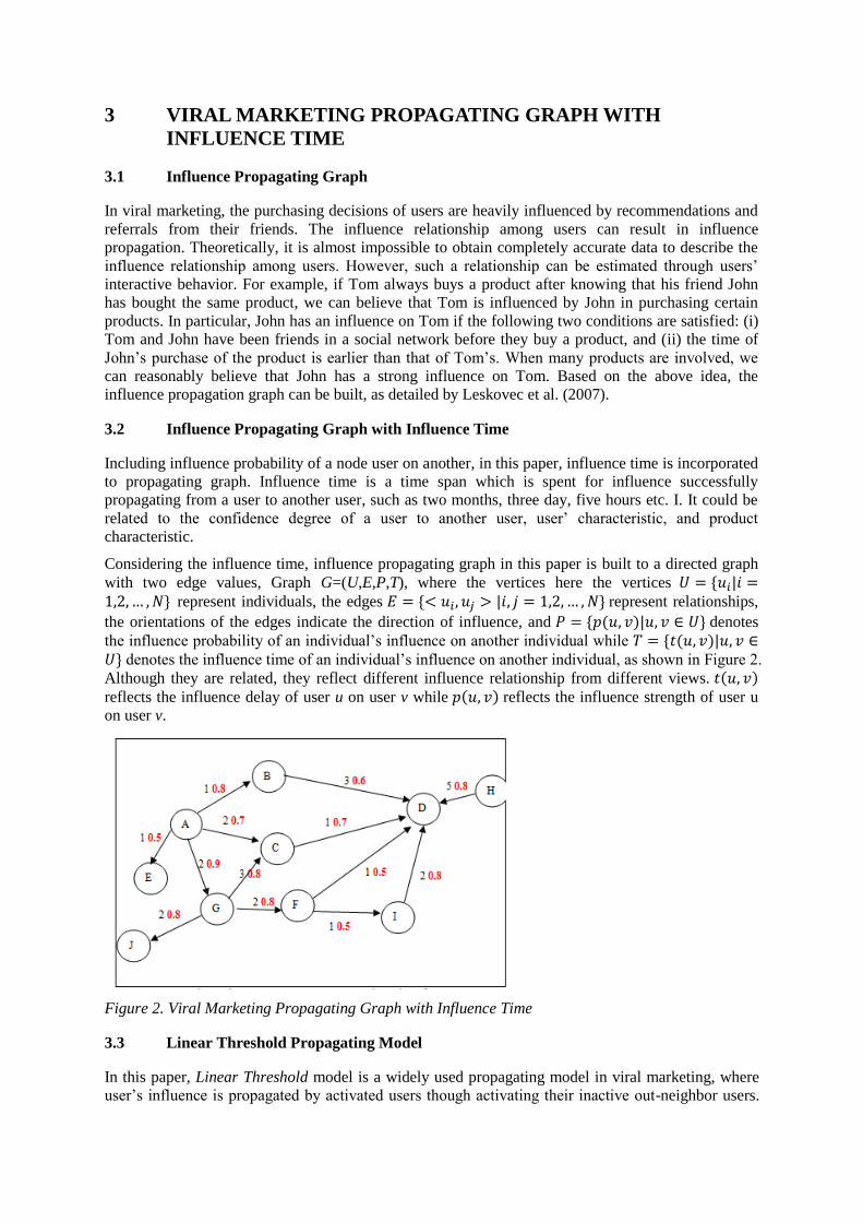
Considering the influence time, influence propagating graph in this paper is built to a directed graph

with two edge values, Graph G=(U,E,P,T), where the vertices here the vertices represent individuals, the edges represent relationships,

the orientations of the edges indicate the direction of influence, and denotes

the influence probability of an individual’s influence on another individual while denotes the influence time of an individual’s influence on another individual, as shown in Figure 2.

Although they are related, they reflect different influence relationship from different views.

reflects the influence delay of user u on user v while reflects the influence strength of user u

on user v.

Figure 2. Viral Marketing Propagating Graph with Influence Time

3.3 Linear Threshold Propagating Model

In this paper, Linear Threshold model is a widely used propagating model in viral marketing, where

user’s influence is propagated by activated users though activating their inactive out-neighbor users.

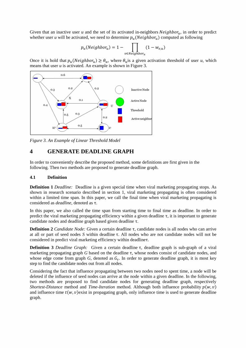
Given that an inactive user u and the set of its activated in-neighbors , in order to predict

whether user u will be activated, we need to determine computed as following

∏

Once it is hold that , where is a given activation threshold of user u, which

means that user u is activated. An example is shown in Figure 3.

Figure 3. An Example of Linear Threshold Model

4 GENERATE DEADLINE GRAPH

In order to conveniently describe the proposed method, some definitions are first given in the

following. Then two methods are proposed to generate deadline graph.

4.1 Definition

Definition 1 Deadline: Deadline is a given special time when viral marketing propagating stops. As

shown in research scenario described in section 1, viral marketing propagating is often considered

within a limited time span. In this paper, we call the final time when viral marketing propagating is

considered as deadline, denoted as .

In this paper, we also called the time span from starting time to final time as deadline. In order to

predict the viral marketing propagating efficiency within a given deadline , it is important to generate

candidate nodes and deadline graph based given deadline .

Definition 2 Candidate Node: Given a certain deadline , candidate nodes is all nodes who can arrive

at all or part of seed nodes S within deadline . All nodes who are not candidate nodes will not be

considered in predict viral marketing efficiency within deadline .

Definition 3 Deadline Graph: Given a certain deadline , deadline graph is sub-graph of a viral

marketing propagating graph G based on the deadline , whose nodes consist of candidate nodes, and

whose edge come from graph G, denoted as . In order to generate deadline graph, it is most key

step to find the candidate nodes out from all nodes.

Considering the fact that influence propagating between two nodes need to spent time, a node will be

deleted if the influence of seed nodes can arrive at the node within a given deadline. In the following,

two methods are proposed to find candidate nodes for generating deadline graph, respectively

Shortest-Distance method and Time-Iteration method. Although both influence probability and influence time exist in propagating graph, only influence time is used to generate deadline

graph.

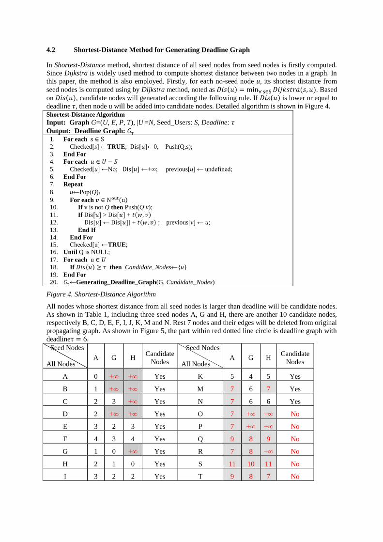
4.2 Shortest-Distance Method for Generating Deadline Graph

In Shortest-Distance method, shortest distance of all seed nodes from seed nodes is firstly computed.

Since Dijkstra is widely used method to compute shortest distance between two nodes in a graph. In

this paper, the method is also employed. Firstly, for each no-seed node u, its shortest distance from

seed nodes is computed using by Dijkstra method, noted as . Based

on , candidate nodes will generated according the following rule. If is lower or equal to

deadline , then node u will be added into candidate nodes. Detailed algorithm is shown in Figure 4.

Shortest-Distance Algorithm

Input: Graph G=(U, E, P, T), |U|=N, Seed_Users: S, Deadline:

Output: Deadline Graph:

1. For each s S

2. Checked[s] ←TRUE; D s[ ]←0; Push(Q,s);

3. End For

4. For each 𝑆

5. Checked[u] ←No; D s[ ] ←+∞; previous[u] ← undefined;

6. End For

7. Repeat

8. u←Pop(Q)；

9. For each Nout u 10. If v is not Q then Push(Q,v);

11. If D s[ ] > D s[ ] +

12. D s[ ] ← D s[ ]] + ; previous[v] ← u;

13. End If

14. End For

15. Checked[u] ←TRUE;

16. Until Q is NULL;

17. For each u

18. If then Candidate_Nodes←{u}

19. End For

20. ←Generating_Deadline_Graph(G, Candidate_Nodes)

Figure 4. Shortest-Distance Algorithm

All nodes whose shortest distance from all seed nodes is larger than deadline will be candidate nodes.

As shown in Table 1, including three seed nodes A, G and H, there are another 10 candidate nodes,

respectively B, C, D, E, F, I, J, K, M and N. Rest 7 nodes and their edges will be deleted from original

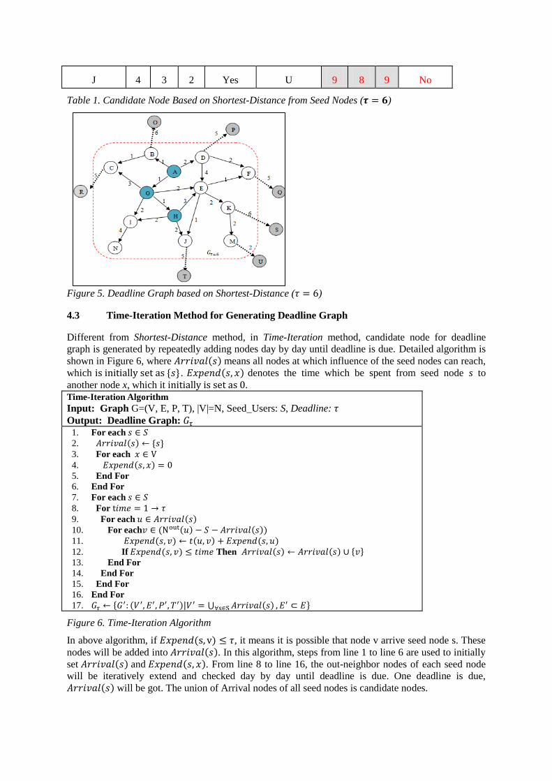
propagating graph. As shown in Figure 5, the part within red dotted line circle is deadline graph with

deadline .

Seed Nodes

All Nodes A G H

Candidate

Nodes

Seed Nodes

All Nodes A G H

Candidate

Nodes

A 0 +∞ +∞ Yes K 5 4 5 Yes

B 1 +∞ +∞ Yes M 7 6 7 Yes

C 2 3 +∞ Yes N 7 6 6 Yes

D 2 +∞ +∞ Yes O 7 +∞ +∞ No

E 3 2 3 Yes P 7 +∞ +∞ No

F 4 3 4 Yes Q 9 8 9 No

G 1 0 +∞ Yes R 7 8 +∞ No

H 2 1 0 Yes S 11 10 11 No

I 3 2 2 Yes T 9 8 7 No

J 4 3 2 Yes U 9 8 9 No

Table 1. Candidate Node Based on Shortest-Distance from Seed Nodes ( )

Figure 5. Deadline Graph based on Shortest-Distance ( )

4.3 Time-Iteration Method for Generating Deadline Graph

Different from Shortest-Distance method, in Time-Iteration method, candidate node for deadline

graph is generated by repeatedly adding nodes day by day until deadline is due. Detailed algorithm is

shown in Figure 6, where means all nodes at which influence of the seed nodes can reach,

which s t set s . denotes the time which be spent from seed node s to

another node x, which it t s set s .

Time-Iteration Algorithm

Input: Graph G=(V, E, P, T), |V|=N, Seed_Users: S, Deadline:

Output: Deadline Graph:

1. For each 𝑆

2. ← 3. For each V

4.

5. End For

6. End For

7. For each 𝑆

8. For t 𝑚 → 9. For each

10. For each Nout 𝑆 11. ← +

12. If ≤ 𝑚 Then ← ∪ 13. End For

14. End For

15. End For

16. End For

17. ← ′: 𝑉′ ′ ′ ′ 𝑉′ ⋃ ′ ⊂

Figure 6. Time-Iteration Algorithm

In above algorithm, if s v ≤ , it means it is possible that node v arrive seed node s. These

nodes will be added into . In this algorithm, steps from line 1 to line 6 are used to initially

set and . From line 8 to line 16, the out-neighbor nodes of each seed node

will be iteratively extend and checked day by day until deadline is due. One deadline is due,

will be got. The union of Arrival nodes of all seed nodes is candidate nodes.

Let’s look an example again as shown in Figure 5. Also supposed that deadline is set as days.

As done by Time-Iteration algorithm, starting from seed nodes, seed node A can arrive at node A and

B after one day while it can arrive node A, B, C and D after two days. After deadline, the seed node A

can arrive 6 nodes, that is to say, {A、B、C、D、F、E}, as shown in Table 2.

Time

0 A G H

1 A、B G H

2 A、B、C、D G、I、E H、I、J

3 A、B、C、D G、I、E、F、J、C H、I、J、E、

4 A、B、C、D、F G、I、E、F、J、C、K H、I、J、E、F

5 A、B、C、D、F G、I、E、F、J、C、K、M H、I、J、E、F、K

6 A、B、C、D、F、E G、I、E、F、J、C、K、M、N H、I、J、E、F、K、N

Candidate Nodes {A, B, C, D, E, F, G, H, I, J, K, L, M, N}= ∪ ∪

Table 2. Arrival Nodes of Seed Node A Within Deadline Based on Time-Iteration

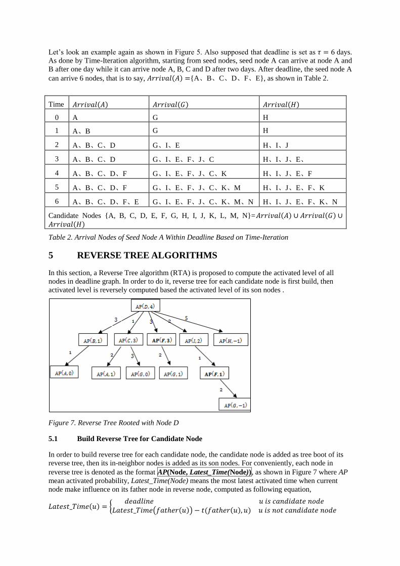
5 REVERSE TREE ALGORITHMS

In this section, a Reverse Tree algorithm (RTA) is proposed to compute the activated level of all

nodes in deadline graph. In order to do it, reverse tree for each candidate node is first build, then

activated level is reversely computed based the activated level of its son nodes .

Figure 7. Reverse Tree Rooted with Node D

5.1 Build Reverse Tree for Candidate Node

In order to build reverse tree for each candidate node, the candidate node is added as tree boot of its

reverse tree, then its in-neighbor nodes is added as its son nodes. For conveniently, each node in

reverse tree is denoted as the format AP(Node, Latest_Time(Node)), as shown in Figure 7 where AP

mean activated probability, Latest_Time(Node) means the most latest activated time when current

node make influence on its father node in reverse node, computed as following equation,

𝑚 {

𝑚 ( )

For example, supposed deadline , in reverse tree rooted by candidate node D, the node D is

denoted as , and its son node B will be denoted as A because the time be delayed 3

day when the influence of node B arrive at node D. That is to say, if activated probability of node D

within deadline wants to be computed, then activated probability of its son node B within 1 day (4

days – 3 days) must be firstly computed. In fact, in the example, in order to compute , we

need to compute , , , and Starting from

candidate node, its son nodes are travelled by breadth-first-search until the most latest activated time

of a node is zero or negative.

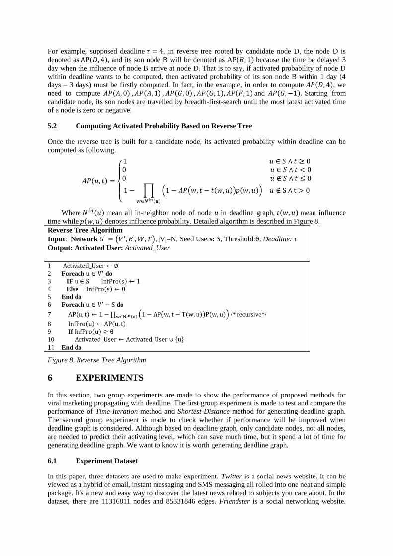
5.2 Computing Activated Probability Based on Reverse Tree

Once the reverse tree is built for a candidate node, its activated probability within deadline can be

computed as following.

{

𝑆 𝑆 𝑆 ≤

∏ ( ( ) )

S t

Where mean all in-neighbor node of node u in deadline graph, mean influence

time while denotes influence probability. Detailed algorithm is described in Figure 8.

Reverse Tree Algorithm

Input: Network (𝑉′ ), |V|=N, Seed Users: S, Threshold: , Deadline:

Output: Activated User: Activated_User

1 ct v ted User ← ∅

2 Foreach u V′ do

3 IF u S I f ro s ←

4 Else I f ro s ←

5 End do

6 Foreach u V′ S do

7 u t ← ∏ ( (w t T w u ) w u )w Nin u /* recursive*/

8 I f ro u ← u t

9 If I f ro u

10 ct v ted User ← ct v ted User ∪ u 11 End do

Figure 8. Reverse Tree Algorithm

6 EXPERIMENTS

In this section, two group experiments are made to show the performance of proposed methods for

viral marketing propagating with deadline. The first group experiment is made to test and compare the

performance of Time-Iteration method and Shortest-Distance method for generating deadline graph.

The second group experiment is made to check whether if performance will be improved when

deadline graph is considered. Although based on deadline graph, only candidate nodes, not all nodes,

are needed to predict their activating level, which can save much time, but it spend a lot of time for

generating deadline graph. We want to know it is worth generating deadline graph.

6.1 Experiment Dataset

In this paper, three datasets are used to make experiment. Twitter is a social news website. It can be

viewed as a hybrid of email, instant messaging and SMS messaging all rolled into one neat and simple

package. It's a new and easy way to discover the latest news related to subjects you care about. In the

dataset, there are 11316811 nodes and 85331846 edges. Friendster is a social networking website.

The service allows users to contact other members, maintain those contacts, and share online content

and media with those contacts. This is the data set crawled by Stephen Booher

([email protected]) on Nov, 2010 from Friendster. It includes 100199 nodes and 14067887

edges. In addition to Twitter and Friendster dataset, a Random dataset is randomly generated for our

experiments.

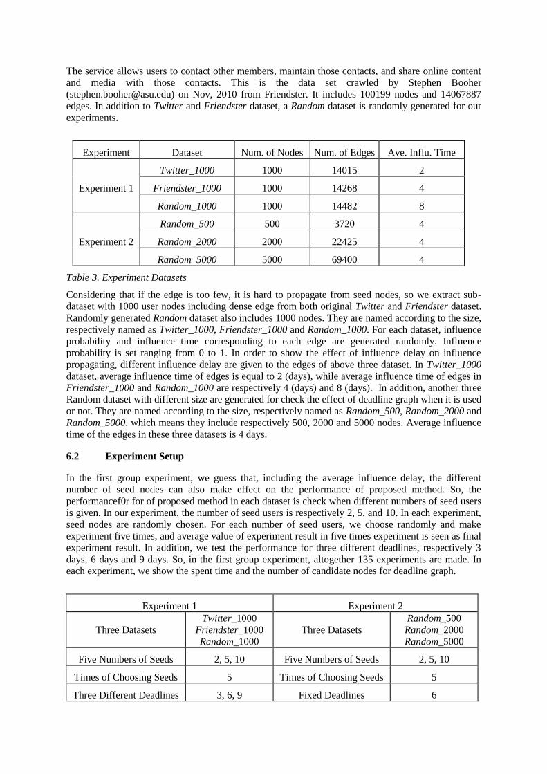
Experiment Dataset Num. of Nodes Num. of Edges Ave. Influ. Time

Experiment 1

Twitter_1000 1000 14015 2

Friendster_1000 1000 14268 4

Random_1000 1000 14482 8

Experiment 2

Random_500 500 3720 4

Random_2000 2000 22425 4

Random_5000 5000 69400 4

Table 3. Experiment Datasets

Considering that if the edge is too few, it is hard to propagate from seed nodes, so we extract sub-

dataset with 1000 user nodes including dense edge from both original Twitter and Friendster dataset.

Randomly generated Random dataset also includes 1000 nodes. They are named according to the size,

respectively named as Twitter_1000, Friendster_1000 and Random_1000. For each dataset, influence

probability and influence time corresponding to each edge are generated randomly. Influence

probability is set ranging from 0 to 1. In order to show the effect of influence delay on influence

propagating, different influence delay are given to the edges of above three dataset. In Twitter_1000

dataset, average influence time of edges is equal to 2 (days), while average influence time of edges in

Friendster_1000 and Random_1000 are respectively 4 (days) and 8 (days). In addition, another three

Random dataset with different size are generated for check the effect of deadline graph when it is used

or not. They are named according to the size, respectively named as Random_500, Random_2000 and

Random_5000, which means they include respectively 500, 2000 and 5000 nodes. Average influence

time of the edges in these three datasets is 4 days.

6.2 Experiment Setup

In the first group experiment, we guess that, including the average influence delay, the different

number of seed nodes can also make effect on the performance of proposed method. So, the

performancef0r for of proposed method in each dataset is check when different numbers of seed users

is given. In our experiment, the number of seed users is respectively 2, 5, and 10. In each experiment,

seed nodes are randomly chosen. For each number of seed users, we choose randomly and make

experiment five times, and average value of experiment result in five times experiment is seen as final

experiment result. In addition, we test the performance for three different deadlines, respectively 3

days, 6 days and 9 days. So, in the first group experiment, altogether 135 experiments are made. In

each experiment, we show the spent time and the number of candidate nodes for deadline graph.

Experiment 1 Experiment 2

Three Datasets

Twitter_1000

Friendster_1000

Random_1000

Three Datasets

Random_500

Random_2000

Random_5000

Five Numbers of Seeds 2, 5, 10 Five Numbers of Seeds 2, 5, 10

Times of Choosing Seeds 5 Times of Choosing Seeds 5

Three Different Deadlines 3, 6, 9 Fixed Deadlines 6

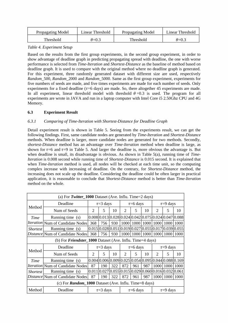
Propagating Model Linear Threshold Propagating Model Linear Threshold

Threshold =0.3 Threshold =0.3

Table 4. Experiment Setup

Based on the results from the first group experiments, in the second group experiment, in order to

show advantage of deadline graph in predicting propagating spread with deadline, the one with worse

performance is selected from Time-Iteration and Shortest-Distance as the baseline of method based on

deadline graph. It is used to compare with the original method where no deadline graph is generated.

For this experiment, three randomly generated dataset with different size are used, respectively

Random_500, Random_2000 and Random_5000. Same as the first group experiment, experiments for

five numbers of seeds are made, and five times experiments are made for each number of seeds. Only

experiments for a fixed deadline ( =6 days) are made. So, there altogether 45 experiments are made.

In all experiment, linear threshold model with threshold =0.3 is used. The program for all

experiments are wrote in JAVA and run in a laptop computer with Intel Core i5 2.50Ghz CPU and 4G

Memory.

6.3 Experiment Result

6.3.1 Comparing of Time-Iteration with Shortest-Distance for Deadline Graph

Detail experiment result is shown in Table 5. Seeing from the experiments result, we can get the

following findings. First, same candidate nodes are generated by Time-Iteration and Shortest-Distance

methods. When deadline is larger, more candidate nodes are generated for two methods. Secondly,

shortest-Distance method has an advantage over Time-Iteration method when deadline is large, as

shown for =6 and =9 in Table 5. And larger the deadline is, more obvious the advantage is. But

when deadline is small, its disadvantage is obvious. As shown in Table 5(a), running time of Time-

Iteration is 0.008 second while running time of Shortest-Distance is 0.015 second. It is explained that

when Time-Iteration method is used, all nodes will be checked at each time unit, so the computing

complex increase with increasing of deadline. On the contrary, for Shortest-Distance method, the

increasing does not scale up the deadline. Considering the deadline could be often larger in practical

application, it is reasonable to conclude that Shortest-Distance method is better than Time-Iteration

method on the whole.

(a) For Twitter_1000 Dataset (Ave. Influ. Time=2 days)

Method Deadline =3 days =6 days =9 days

Num of Seeds 2 5 10 2 5 10 2 5 10

Time

Iteration

Running time (s) 0.008 0.013 0.028 0.024 0.042 0.075 0.024 0.047 0.088

Num of Candidate Nodes 368 756 930 1000 1000 1000 1000 1000 1000

Shortest

Distance

Running time (s) 0.015 0.028 0.051 0.019 0.027 0.055 0.017 0.039 0.055


(b) For Friendster_1000 Dataset (Ave. Influ. Time=4 days)


Num of Seeds 2 5 10 2 5 10 2 5 10

Time

Iteration

Running time (s) 0.004 0.006 0.009 0.025 0.054 0.095 0.044 0.088 0.169


Shortest

Distance

Running time (s) 0.011 0.027 0.055 0.015 0.029 0.060 0.016 0.032 0.061


(c) For Random_1000 Dataset (Ave. Influ. Time=8 days)


Num of Seeds 2 5 10 2 5 10 2 5 10

Time

Iteration

Running time (s) 0.003 0.004 0.006 0.012 0.017 0.033 0.048 0.096 0.155


Shortest

Distance

Running time (s) 0.011 0.026 0.062 0.015 0.034 0.050 0.018 0.033 0.065


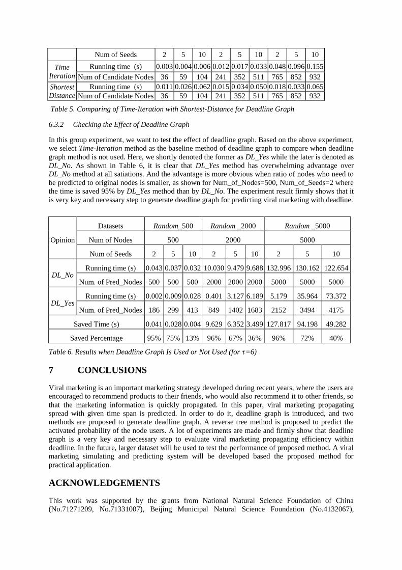
Table 5. Comparing of Time-Iteration with Shortest-Distance for Deadline Graph

6.3.2 Checking the Effect of Deadline Graph

In this group experiment, we want to test the effect of deadline graph. Based on the above experiment,

we select Time-Iteration method as the baseline method of deadline graph to compare when deadline

graph method is not used. Here, we shortly denoted the former as DL_Yes while the later is denoted as

DL_No. As shown in Table 6, it is clear that DL_Yes method has overwhelming advantage over

DL_No method at all satiations. And the advantage is more obvious when ratio of nodes who need to

be predicted to original nodes is smaller, as shown for Num_of_Nodes=500, Num_of_Seeds=2 where

the time is saved 95% by DL_Yes method than by DL_No. The experiment result firmly shows that it

is very key and necessary step to generate deadline graph for predicting viral marketing with deadline.

Opinion

Datasets Random_500 Random _2000 Random _5000

Num of Nodes 500 2000 5000

Num of Seeds 2 5 10 2 5 10 2 5 10

DL_No Running time (s) 0.043 0.037 0.032 10.030 9.479 9.688 132.996 130.162 122.654

Num. of Pred_Nodes 500 500 500 2000 2000 2000 5000 5000 5000

DL_Yes Running time (s) 0.002 0.009 0.028 0.401 3.127 6.189 5.179 35.964 73.372

Num. of Pred_Nodes 186 299 413 849 1402 1683 2152 3494 4175

Saved Time (s) 0.041 0.028 0.004 9.629 6.352 3.499 127.817 94.198 49.282

Saved Percentage 95% 75% 13% 96% 67% 36% 96% 72% 40%

Table 6. Results when Deadline Graph Is Used or Not Used (for =6)

7 CONCLUSIONS

Viral marketing is an important marketing strategy developed during recent years, where the users are

encouraged to recommend products to their friends, who would also recommend it to other friends, so

that the marketing information is quickly propagated. In this paper, viral marketing propagating

spread with given time span is predicted. In order to do it, deadline graph is introduced, and two

methods are proposed to generate deadline graph. A reverse tree method is proposed to predict the

activated probability of the node users. A lot of experiments are made and firmly show that deadline

graph is a very key and necessary step to evaluate viral marketing propagating efficiency within

deadline. In the future, larger dataset will be used to test the performance of proposed method. A viral

marketing simulating and predicting system will be developed based the proposed method for

practical application.

ACKNOWLEDGEMENTS

This work was supported by the grants from National Natural Science Foundation of China

(No.71271209, No.71331007), Beijing Municipal Natural Science Foundation (No.4132067),

Humanity and Social Science Youth Foundation of Ministry of Education of China

(No.11YJC630268), Special Fund for Fast Sharing of Science Paper in Net Era by CSTD

(No.2013112), Opening Project of State Key Laboratory of Digital Publishing Technology,

Fundamental Research Funds for the Central Universities, and the Research Funds of Renmin

University of China.

References

Arthur, D. Motwani, R., Sharma, A., Xu, Y., (2009). "Pricing Strategies for Viral Marketing on Social

Networks," in Proceedings of the 5th International Workshop on Internet and network economics.

Verlag Berlin, Heidelberg pp. 101-112.

Bruyna, A.D., Lilien, G.L., (2008). "A Multi-stage Model of Word-of-mouth Influence through Viral

Marketing," International Journal of Research in Marketing. (25:3), pp. 151-163.

Cao, J.W., Knotts, T., Xu, J., Chau, M., (2009). "Word of Mouth Marketing through Online Social

Networks," In Proceedings of American Conference on Information System. pp. 291-292.

Chen, W., Wang, C. and Wang, Y., (2010). "Scalable Influence Maximization for Prevalent Viral

Marketing in Large-scale Social Networks," In Proceeding of the ACM International Conference

on knowledge discovery and data mining, PP.1029–1038.

Goyal, A., Bonchi, F., Lakshmanan, L., (2008). "Discovering Leaders from Community Actions," In

Proceeding of the 17th ACM conference on information and knowledge management. pp. 179-

182.

Iribarren, J. L., and Moro, E. (2009). "Impact of Human Activity Patterns on the Dynamics of

Information Diffusion," Physics Review Letters 103:038702.

Immorlica, N., Mirrokni, V., (2010). "Optimal Marketing and Pricing Over Social Networks," In

Proceedings of the 19th International World Wide Web conference. pp. 1349-1350.

Karsai, M., Kivel a, M., Pan, R. K., Kaski, K., Kert esz, J.;Barab asi, A.-L. and Saram aki, J. (2011).

"Small But Slow World: How Network Topology and Burstiness Slow Down Spreading," Physics

Review Letters 83:025102.

Kempe, D., Kleinberg, J., Tardos, E., (2003). "Maximizing the Spread of Influence Through A Social

Network," In Proceedings of the 9th ACM SIGKDD international conference on knowledge

discovery and data mining, pp. 137-146.

Kiss, C., G. and Rusinowska M., (2008). "Identification of Influencers-Measuring Influence in

Customer Networks," Decision Support Systems. (46:1), pp. 233-253.

Leskovec, J., Krause, A., Guestrin, C., Faloutsos, C., VanBriesen, J., Glance, N.S., (2007). "Cost-

effective Outbreak Detection in Networks," In Proceeding of the 13th ACM International

Conference on knowledge discovery and data mining. pp. 420-429.

Leskovec, J., Adamic, L., Huberman, B., (2006). "The Dynamics of Viral Marketing," In Proceedings

of the 7th ACM conference on Electronic Commerce. pp. 228-237.

Li, Y., Lin, C., Lai, C., (2010). "Identifying Influential Reviewers for Word-Of-Mouth Marketing,"

Electronic Commerce Research and Applications. (9:4), pp. 294-304.

Li, Y., Qiulin, L., Xun, L., (2012). "Research on Viral Marketing Propagating Oriented to Marketing

Context," In Proceedings of International Conference on Information System, Orlando Florida

USA

Trusov, M., Boapati, A., Bucklin, R. (2010). "Determining Influential Users in Internet Social

Networks," Journal of Marketing Research, (47:4), pp. 643-658.

Wei, C., Wei, L. and Ning, Z., (2012). "Time-critical Influence Maximization in Social Networks

with Time Delayed diffusion Process," In Proceedings of the 26th Conference on Artificial

Intelligence, Toronto, Canada,

predicting viral marketing propagating efficiency within ... · pdf filepredicting viral...

Documents