1

PREDICTING THE FACTOR CONTENT OF TRADE: THEORY AND EVIDENCE1

Daniel M. Bernhofen2

School of Economics and GEP

University of Nottingham

January 27, 2007

PRELIMINARY DRAFT

Abstract

This paper examines the multi-cone specification of the factor proportion theory of

international trade. I show that Helpman’s bilateral restrictions on the factor of content of trade, which have found recent empirical support by Choi and Krishna (2004), need to be amended to account for multilateralism. I identify additional restrictions and show that these restrictions form the building block for a multi-lateral specification which extends Alan Deardorff’s two-country, two-factor, multiple goods chain of comparative advantage prediction to multiple countries and factors. Applying Choi and Krishna’s data set to the multi-lateral specification, I find little empirical support for the prediction of the model. “It is not possible through merely bilateral comparison to develop a…theory of

efficient multilateral specialization”. (Lionel McKenzie, 1954, p. 180)

1. Introduction

In a recent paper Choi and Prishna (2004) claim to provide a significant

advancement in testing the Heckscher-Ohlin theory of international trade. The authors

provide empirical support for a prediction on the bilateral factor content of trade,

originally developed by Helpman (1984). Helpman’s bilateral specifications have the

attractive features of relying on ‘post-trade’ factor price comparisons and claim to

1 I am grateful to Pravin Krishna for providing me access to the data set used in Choi and Krishna (2004). 2 Address for Correspondence: School of Economics and Leverhulme Centre for Research on Globalization and Economic Policy, University of Nottingham, University Park, Nottingham, NG7 2 RD, UK. Tel: 44 115 846 7055, Fax: 44 115 951 4159, email: daniel.bernhofen@nottingham.ac.uk.

2

hold under nonequalization of factor prices and in the absence of any assumptions

regarding consumer preferences.3

This paper makes two contributions. On the theoretical side, I show that

Helpman’s (1984) prediction in which the bilateral trade flows between country’s i

and j are predicted solely by the factor price difference between these two countries is

an inappropriate Heckscher-Ohlin specification in a multi-country world. The

intuition for this is that in Helpman’s formulation factor prices embody information

about a country’s underlying factor scarcities. As a result, a prediction on the pattern

of trade between countries i and j must also incorporate information about the relative

factor prices of any third country k. In fact, in a general trading equilibrium the

pattern of international specialization must be predicted by factor scarcity measures of

all trading partners.

Building on Helpman’s proof for deriving bilateral restrictions, I incorporate

multi-lateralism into the model. I identify additional restrictions that have to hold in

a trading equilibrium. I show that these restrictions define country-specific cones of

diversification where the theory predicts that the factor content of any export flow,

bilateral or multilateral, must lie within this cone. This specification extends Alan

Deardorff’s (1979) well-known two-country, two-factor, multiple goods chain of

comparative advantage prediction to multiple factors and countries.

In the second part of the paper, I apply Choi and Krishna’s (2004) data set to

the theory. In general, I find little empirical support for the multi-cone specifiation.

With the exception of the two countries who occupy a boundary cone, none of the

other countries’ exports fall into the correct cone. When testing the restrictions

individually, I find that the success rate is as good as the toss of a coin.

The paper is organized as follows. Section 2 revisits Helpman (1984) and

shows that Helpman’s prediction will coincide with Deardorff’s (1979) multi-cone

chain of comparative prediction only in the two-country case. Section 3 derives the

multi-cone specification of the Heckscher-Ohlin model in the case of multiple

countries. Section 4 provides a brief summary of Choi and Krishna’s (2004) data set.

Section 5 gives the empirical results and section 6 contains the conclusion.

3 Helpman and Krugman (1985, pp. 24-27) and Feenstra (2004, pp.58-60) provide detailed discussions of Helpman (1984); Staiger (1986) extends Helpman’s analysis to deal with intermediates. Building on Choi and Krishna (2004), Lai and Zhu (2006) provide further empirical support for a modified prediction that incorporates technological differences.

3

2. Revisiting the chain of comparative advantage

Helpman’s specification aims to extend Deardorff’s (1979) and Brecher and

Choudhri’s (1982) two-country, two-factor “chain formulation” to multiple countries

and factors. The central theme in these papers is to provide predictions in the spirit of

Heckscher-Ohlin, but in the absence of factor price equalization. All three papers

investigate the property of a competitive free trade equilibrium with two key

characteristics. First, all countries possess identical production functions. Second,

countries’ factor endowments are assumed to be sufficiently dissimilar so that

countries’ free trade factor prices are different.

Formally, consider a competitive equilibrium with m countries, n goods, l

factors and a common technology matrix, A(.)=<aντ(.)>, where aντ are the units of

factor ν necessary to produce 1 unit of good τ. Although identical technologies imply

the same functional forms for aντ, the equilibrium least-cost input coefficients will

depend on country specific factor prices.

If Tij denotes the vector of gross imports of country j from country i, Fij

denotes the factor content of Tij evaluated at the exporter’s input techniques, i.e.

Fij=A(wi)Tij, where wi is the free-trade factor price vector of the exporting country i.

For two countries, i and j, who are engaged in bilateral trade, Helpman (1984) derives

the following prediction on the bilateral factor content of trade Fij:

(wj-wi)'Fij ≥ 0. (1)

By symmetry, we obtain an equivalent prediction on the gross trade flow from

country j to country i:

(wi-wj)'Fji ≥ 0. (2)

Adding (1) and (2) results in a bilateral prediction on the net trade flow between

countries i and j:

(wj-wi)'(Fij-Fji) ≥ 0. (3)

Inequality (3) has been interpreted as saying that factors embodied in trade

should flow towards the country with the higher factor price. If factor ν has a higher

4

absolute price in country j, wjν-wi

ν >0, then j will, ”on average”, be a net importer of

that factor relative to country i, i.e. Fijν- Fji

ν > 0.

However, the predictions in (1)-(2) seem to be at odds with the fact that in a

general equilibrium with multiple countries, any trade flow must be determined by

relative measures of factor scarcities of all trading partners. In particular, the

predictions on Fij and Fji take into account only information on bilateral factor price

differences of the two trading partners, without considering the factor prices of any

other third countries. In what follows, I will show that (1)-(2) generalizes Brecher

and Choudhri’s (1982) factor content version of Heckscher-Ohlin to multiple factors,

but not to multiple countries.

Figure 1: Multi-cone commodity-content prediction

Figure 1 depicts the Lerner-Pearce diagram for the case of 6 goods, 2 factors

(labour and capital) and 3 countries. The goods’ isoquants, numbered from 1 to 6,

depict the input combinations that can produce $1 worth of output at the free trade

prices. The goods numbering pertains to their capital-intensity ranking, where good 1

is most capital-intensive and good 6 is least capital-intensive. The rays (K/L)i denote

the countries’ capital labour ratios and ωi (=(wi/ri)) represent the countries’ free trade

5

wage-rental ratios (i=1,..3). The implicit assumption behind this specification is that

there is a one-to-one correspondence between the factor endowment ranking and the

ranking of free trade equilibrium factor price ratios ωi (=(wi/ri)): (K/L)1 > (K/L)2 >

(K/L)3 <=> (w1/r1) > (w2/r2) > (w3/r3). In any pair-wise comparison, the more

capital-abundant country is expected to have a higher equilibrium wage-rental ratio.

Since countries’ factor endowments are assumed to be in different cones of

diversification, the three countries will specialize in the production of different

goods.4 In a trading equilibrium, the most capital-abundant country 1 will produce

and export the most capital-intensive goods 1 and 2; country 2 will produce and

export goods 3 and 4 and the most labour abundant country 3 will produce and export

the most labour-intensive goods 5 and 6.5 This is the Heckscher-Ohlin commodity-

chain prediction, which goes back to Jones (1956-57), Bhagwati (1972) and Deardorff

(1979).

Alternatively, instead of considering the pattern of commodity trade, this

framework makes also predictions on factor content of trade. In reference to Figure 1,

Helpman (1984, p. 90) writes:

“It is now a simple matter to observe that the more capital-rich a country is,

the more capital and less labour is uses per dollar output in all lines of production

(more generally, it never uses less capital and more labour). Hence, whatever trade

there may exist between two countries, exports of the relatively capital rich country

will embody a higher capital-labour ratio than exports of the relatively labour rich

country. This describes a clear bilateral factor content pattern of trade (see Brecher

and Choudhri, 1982)”.

The key point here is that the factor content comparison pertains to all exports

by countries i and j: bilateral, multi-lateral, and independent of destination.

Consequently, the emphasis of (1)-(3) on bilateral trade is misleading, unless we are

in Brecher and Choudhri’s (1982) two-country framework where there is no

distinction between bilateral and multi-lateral trade.

4 There are three cones of diversification, defined by the lines (not drawn) between the origin and the 6 depicted tangencies. 5 Although this framework doesn’t make any explicit assumption about preferences, it implicitly assumes that preferences are such that the free trade equilibrium actually exists. In particular, to ensure that there is some trade, one needs to assume that consumers care about foreign-produced goods.

6

Let Ti denote any equilibrium export flow by country i . The corresponding

factor content of exports is then defined as Fi=A(wi)Ti. In the two-factor case, the

factor content prediction is given by:

3

3

2

2

1

1

LK

LK

LK

≥≥ , (4)

where Fi=(Ki,Li) is any factor content of export vector for country i. The prediction in

(4) is the factor content version of the commodity prediction from Figure 1.

Geometrically, it corresponds to a three-cone partitioning (C1, C2, C3) of the labour-

capital space, where the cones are defined by the equilibrium capital-labour ratios of

the respective commodities. Figure 2 illustrates that the theory predicts that Fi∈ Ci for

all i. For example, any factor content of exports vector F1 of country 1 must have a

capital-labour ratio that is higher than its least-capital-intensive good, i.e. good 2. The

capital-labour ratio of any export vector F2 of country 2 must be between the capital-

labour ratios of good 2 and good 4 and the capital-labour ratio of any export vector F3

of country 3 must be lower than the capital-labour ratio of good 4.

Figure 2: Multi-cone factor-content prediction

C2

L

KC1

F1

F2

F3C3

7

We can compare this now to Helpman’s predictions (1)-(2). Assuming that

country i is capital abundant relative to country j, i.e. wi/ri > wj/rj, (1) and (2) lead to

the following inequalities6:

ji

ji

ij

ji

ij

ij

LK

rrww

LK

≥−

−≥ (5)

Figure 3: Helpman’s bilateral ‘two-cone specification’

Figure 3 captures (5) geometrically and illustrates the difference to the multi-

cone specification given in Figure 2. In the case of three countries, Helpman’s

predictions correspond to three different two-cone partitionings (Cij, Cji) of the labour-

capital space, one for each country pair. It is immediately clear that (5) will coincide

with the multi-cone specification only in a two-country world.

3. Deriving multi-cone factor content of trade predictions

In this section I derive general factor content of trade predictions and show

that they generalize the predictions in Figure 2 to multiple factors and countries. I

accomplish this by using Helpman’s strategy for deriving (1) and (2). Helpman

arrives at (1) through two steps: (i) a ‘thought experiment’ on a factor endowment gift

6 Without loss of generality we have assumed that wi>wj. The identical technology assumption implies then that rj>ri , which guarantees that the ratio of factor price differences is positive.

Cji

L

KCij

Fij

Fji

(wi-wj)/(rj-ri)

8

and (ii) the concavity property of GDP function.7 In a free trade equilibrium a

country’s GDP can be written as G(p,Vj)= p′Yj=wj′ Vj, where Vj denotes the country’s

endowment vector, Yj its production vector and p the free trade equilibrium goods

price vector. Helpman postulates then the following relationships:

wiFij =pTij ≤ G(p,Vj+Fij)-G(p,Vj), (6)

G(p,Vj+Fij)-G(p,Vj) ≤ wj′ Fij. (7)

Inequalities (6) and (7) can be interpreted as providing lower and upper bounds for

gain in revenue, G(p,Vj+Fij)-G(p,Vj), economy j would obtain from a hypothetical

endowment gift of Fij. Inequality (7) follows directly from the concavity property of

the GDP function: the gain in revenue must be smaller than the gift Fij valued at the

shadow price wj associated with Vj. Inequality (6) is based on factor price

differences between countries. If country j were given a factor endowment gift of Fij,

then the assumption of identical technologies implies that it would be feasible for

country j to produce Tij itself and obtain the revenue p′ Tij.8 However, since factor

prices in country j are different than in i, country j could do ‘potentially better’ than

that. Consequently p′ Tij provides a lower bound for the revenue gain G(p,Vj+Fij)-

G(p,Vj). Using the zero-profit condition, p′ Tij=wi′ Fij, and combining (6) and (7), we

obtain (1).

However, it has remained unnoticed that the underlying logic applies to any

other third country k and to any exports by country i. Consider any export vector Ti by

country i. For example, if country k were given an endowment gift of Fi=A(wi)Ti, the

country’s increase in GDP, G(p,Vk+Fi)-G(p,Vk), would be at least as large as p′ Ti, i.e.

wiFi = pTi ≤ G(p,Vk+Fi)-G(p,Vk). (8)

On the other hand, the endowment gift Fi evaluated at country k’s equilibrium

or shadow price vector wk provides an upper bound for the revenue gain of country k:

G(p,Vk+Fi)-G(p,Vk) ≤ wk′ Fi. (9)

7 In what follows, I revisit Helpman’s proof by adopting the user-friendly notation used by Feenstra (2004, p. 58-59). 8 It is implicitly assumed that the factor reallocation does not affect the equilibrium price vector p.

9

Combining (8) and (9), one obtains

(wk-wi)'Fi ≥ 0, for all k≠i, (10)

Inequality (10), which is the main theoretical result of this paper, differs from

Helpman’s bilateral prediction (1) in two ways. First, it yields predictions on the

factor content of all exports by country i, bilateral and multilateral. Second, each

factor content of exports Fi is restricted by the difference between the factor price in i

and the factor price in each of its (m-1) trading partners. The intuition behind (10) is

that in this specification of the neoclassical trade model, free trade factor prices

embody information about countries’ underlying factor scarcities. As a result, in a

world with more than 2 countries, a factor flow between countries i and j can’t be

accurately predicted by using only information about factor scarcities of countries i

and j, but must incorporate factor price information of all trading partners.

The restrictions in (10) can be viewed as defining a country-specific cone Ci in

the factor endowment space,

Ci= Iik≠

{F∈Rl | (wk-wi)F ≥ 0} (11)

where the theory predicts that Fi∈Ci for any factor content of exports Fi. The key

point here that each cone is constructed by using factor prices of all trading partners,

i.e. Ci=Ci(w1,…wm).

To illustrate that (11) generalizes the factor content prediction of Figure 2, let

us construct Ci in the two-factor, three-country case. We assume, without loss of

generality, that the free trade equilibrium is characterized by a factor price ordering,

w1>w2>w3 and r1<r2<r3, which is compatible with Figure 1. Applying the factor price

data to (11), the cones are given by:

C1={(K,L)| ≥LK max{

13

31

12

21,

rrww

rrww

−

−

−

− }}, (12a)

C2={(K,L}| 23

32

rrww

−

−≤≤

LK

12

21

rrww

−

− }, (12b)

10

C3={(K,L)| ≤LK min{

23

32

13

31,

rrww

rrww

−

−

−

− }}. (12c)

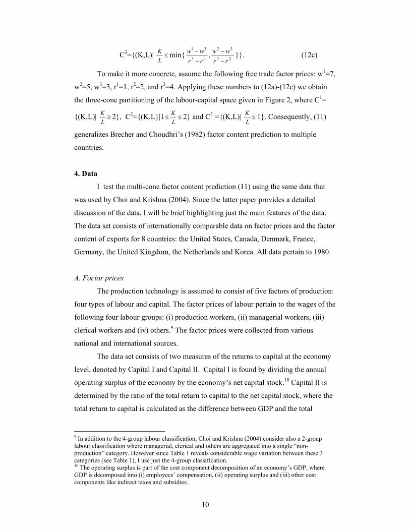
To make it more concrete, assume the following free trade factor prices: w1=7,

w2=5, w3=3, r1=1, r2=2, and r3=4. Applying these numbers to (12a)-(12c) we obtain

the three-cone partitioning of the labour-capital space given in Figure 2, where C1=

{(K,L)| ≥LK 2}, C2={(K,L}|1 ≤≤

LK 2} and C3 ={(K,L)| ≤

LK 1}. Consequently, (11)

generalizes Brecher and Choudhri’s (1982) factor content prediction to multiple

countries.

4. Data

I test the multi-cone factor content prediction (11) using the same data that

was used by Choi and Krishna (2004). Since the latter paper provides a detailed

discussion of the data, I will be brief highlighting just the main features of the data.

The data set consists of internationally comparable data on factor prices and the factor

content of exports for 8 countries: the United States, Canada, Denmark, France,

Germany, the United Kingdom, the Netherlands and Korea. All data pertain to 1980.

A. Factor prices

The production technology is assumed to consist of five factors of production:

four types of labour and capital. The factor prices of labour pertain to the wages of the

following four labour groups: (i) production workers, (ii) managerial workers, (iii)

clerical workers and (iv) others.9 The factor prices were collected from various

national and international sources.

The data set consists of two measures of the returns to capital at the economy

level, denoted by Capital I and Capital II. Capital I is found by dividing the annual

operating surplus of the economy by the economy’s net capital stock.10 Capital II is

determined by the ratio of the total return to capital to the net capital stock, where the

total return to capital is calculated as the difference between GDP and the total

9 In addition to the 4-group labour classification, Choi and Krishna (2004) consider also a 2-group labour classification where managerial, clerical and others are aggregated into a single “non-production” category. However since Table 1 reveals considerable wage variation between these 3 categories (see Table 1), I use just the 4-group classification. 10 The operating surplus is part of the cost component decomposition of an economy’s GDP, where GDP is decomposed into (i) employees’ compensation, (ii) operating surplus and (iii) other cost components like indirect taxes and subsidies.

11

employee compensation. Since Capital I is net of taxes on production, while capital II

is gross of indirect taxes, the latter will provide a higher estimate than the former.

Table 1 reports the factor prices for each factor category and country in US

dollars. The figures suggest quite a bit of factor price variation in the labour

categories across countries. Not surprisingly, Korean wages are the lowest in all

labour categories by a substantial margin. Comparing the Korean wage with the

sample median (which excludes Korea), the Korean wage ranges from 12% (“others”)

to 27% (“managerials”) of this median. Since Korea has also the highest rental price

of capital (for both capital measures) Korea occupies the ‘lower boundary cone’ in

the labour-capital space, i.e. it is the least capital-abundant country.

The contenders for the most capital abundant country are capital-measure

specific: Denmark for Capital I and the US for Capital II. Both take a middle position

in their nominal labour costs (i.e. their labour costs are, on average, below the median

of the sample excluding Korea). Denmark has the lowest rental rate of capital using

Capital I and the US has the lowest rental rate of capital for Capital II. However, the

relative capital abundance is a bit more pronounced for Denmark than for the US:

Capital I for Denmark is 58% of the sample median whereas the Capital II for the US

is only 87% of the sample median.11

Table 1: Factor Prices

Category US Canada Denmark France Germany UK Netherlands KoreaA. Labour (in U.S. Dollars) Production 13,059 12,592 13,333 14,715 18,789 12,595 18,177 1,638Managerial 26,589 21,165 24,985 40,855 34,011 21,011 36,670 7,189Clerical 14,869 11,460 17,313 16,221 16,389 9,323 18,363 2,910Others 21,578 16,960 15,788 22,859 24,544 14,529 25,083 2,495B. Capital Capital I 0.08 0.103 0.053 0.078 0.091 0.075 0.097 0.155Capital II 0.165 0.19 0.174 0.18 0.203 0.203 0.185 0.234Source: Choi and Krishna (2004)

B. Factor content of trade

The factor content of trade vectors are constructed by combining data from a

17 sector ISIC classification with the corresponding country-specific technology

matrices. From the 17 sectors, nine are two-digit manufacturing industries and eight

11 These sample medians are again exclusive of Korea.

12

are one-digit non-manufacturing sectors. The industries and their classification

numbers are listed in Table A1 of the Appendix.

The country-specific technology matrices give the total (direct and indirect)

factor inputs required to produce one dollar of net output in each industry. Each

technology matrix Ac is constructed by multiplying a country’s direct input matrix BC

(factor by industry categorization) with its input-output matrix Ťc (industry by

industry categorization) such that Ac= BC(I- Ťc)-1.12 This specification of the

technology matrix guarantees that the factor content takes into account only

domestically produced intermediate goods.

5. Empirical results

I apply the above data set to predictions on the factor content of gross and net

exports. Section 5.1 contains the empirical results on the factor content of gross

exports and section 5.2. focuses on net trade flows. Although the underlying theory

makes predictions on the pattern of gross exports, we investigate also the implications

for net export flows to allow for a direct comparison with Choi and Krishna (2004).

5.1 Predicting the factor content of gross exports

First, I examine the correct multi-lateral specification (11) and investigate how

many exports fall in the corresponding multi-lateral cone, i.e. fulfill all the

inequalities given in (10). Given that there are 8 countries, we have a sample of 56

bilateral and 8 multi-lateral exports, where the latter is defined as the factor content of

a country’s exports to all 7 trading partners. Table 2 summarizes the results of the

multi-lateral test of the theory. The findings are quite stark. Table 2 reveals that either

all or none of a country’s exports fall in its multi-cone prediction with no systematic

differences between bilateral and multi-lateral trade flows.13

12 The direct input matrix BC measures how much direct input of each factor is required to produce one dollar of gross output in each industry. The input-output matrix Ťc measures how much output an industry must buy from another industry to produce one dollar of its gross output. 13 Since I didn’t find any different results when considering trade flows to a subset of trading partners (e.g. US exports to France and Germany only), I report only the findings for the multi-lateral exports to all sample trading partners.

13

Table 2

Exports falling in the correct multi-lateral cones Capital I Capital II Correct % of total Correct % of total United States 0 0.00 0 0.00Canada 0 0.00 0 0.00Denmark 8 1.00 0 0.00France 0 0.00 0 0.00Germany 0 0.00 0 0.00United Kingdom 0 0.00 0 0.00Netherlands 0 0.00 0 0.00Korea 8 1.00 8 1.00all countries 16 0.25 8 0.125Total of 64 exports (7 bilateral and 1 multi-lateral flow per country)

Overall, the results suggest poor support for the multi-lateral specification: the

success rate is 25% for the capital I measure and 12.5% for the capital II measure.

While all Korean exports are compatible with the predictions, Denish exports fall in

this country’s cone for the capital I measure, but not for the capital II measure; none

of the exports of the other 6 countries fall in the correct cone.

To allow a comparison with Helpman’s bilateral specification, we applied the

data to the bilateral restrictions given in (1). The results are given in Table 3. The

average success rate of the bilateral specification is 55%. Although there is

considerable variation across countries, ranging form 0% (Capital I for Netherlands)

to 100% (Korea), the sample average is the same for both capital measures. Although

the bilateral specification is just based on a single restriction, the success rate is just a

bit over 50%. If we exclude the Korean exports, the bilateral specification is about as

successful as the toss of a coin, i.e. 49%.

Table 3

Exports falling in the (country-pair specific) bilateral cones Capital I Capital II correct % of total correct % of total United States 3 0.43 6 0.86Canada 4 0.57 5 0.71Denmark 7 1.00 5 0.71France 3 0.43 3 0.43Germany 1 0.14 0 0.00United Kingdom 6 0.86 4 0.57Netherlands 0 0.00 1 0.14Korea 7 1.00 7 1.00all countries 31 0.55 31 0.55excluding Korea 24 0.49 24 0.4956 bilateral exports (7 per country); 49 exports excluding Korea

14

Figure 4 provides the basic intuition for the results reported in Table 2 and 3.

The additional restrictions implied by the multi-lateral specification yield much

smaller cones for each country than suggested by the bilateral specification. The high

“success rate” of Korea’s exports in the multi-lateral specification can be explained by

its relative “factor price distinctiveness”, resulting in Korea occupying the relatively

large boundary cone C8 within the capital-labour space. On the other hand, (12b)

suggests that similarity of factor prices corresponds to “middle cones” that are fairly

close to each other and the predictions are not likely to hold.

Figure 4: Multi-cone versus bilateral specification with 8 countries

One might argue that the lack of empirical support for the multi-cone model

might be the result of the relative strictness of the specification in (11) since it

requires that an export flow must fulfil a total of seven restrictions to fall in the

correct multi-lateral cone. However, small measurement errors might prevent this

from happening. To investigate this, we now deviate from grouping the restrictions

into cones and investigate the sign of the restrictions separately. Specifically, we test

the following restrictions on the factor content of bilateral trade

(wk-wi)'Fij ≥ 0, for all j≠i, k≠i. (13)

For 8 countries, (13) implies a total of 49 restrictions for each country: 7

bilateral exports are each restricted by 7 different factor price differences. The results,

which are reported in Table 4, are similar to the numbers reported in Table 3.

Although there is substantial variation across countries, average success rate is 0.57

L

K

L

K

Cij

Cji

Ci

Cj

C1

C8

C2

15

and 0.56 for the Capital I and capital II, respectively. As before, the magnitude of the

average is driven by Korea; excluding Korea, the success rate is about 50%.

Table 4

Summary of sign restrictions on gross exports Capital I Capital II positive % of total Positive % of total United States 26 0.53 42 0.86Canada 28 0.57 41 0.84Denmark 49 1.00 35 0.71France 22 0.45 21 0.43Germany 7 0.14 0 0.00United Kingdom 42 0.86 25 0.51Netherlands 0 0.00 7 0.14Korea 49 1.00 49 1.00all countries 223 0.57 220 0.56excluding Korea 174 0.51 171 0.50392 restrictions (49 per country); 343 restrictions excluding Korea

5.2 Revisiting Choi and Krishna (2004)

In this section we test the multi-lateral restrictions on the two-way trade flows

between countries i and j, which allows for a direct comparison with the research

results in Choi and Krishna (2004). Instead of testing the predictions (1) and (2) on

gross exports Fij and Fji separately, Choi and Krishna test the predictions (3) on net

exports Fij-Fji.14 For ease of interpretation, (3) can be written as follows:

jijiji

jiiijj

FwFwFwFw

++ ≥ 1 (14)

Inequality (14) can be interpeted as follows. For a given country pair, the left-hand

side is the sum of the importer’s counterfactual production costs (using the exporter’s

factor usage and the importer’s factor prices) over the sum of the actual costs of

producing these imports. The theory predicts then that this ratio must be greater than

or equal to 1.

Table A2 in the Appendix contains a replication of Choi and Krishna’s test of

(14). The tests perform remarkably well; the success rate is 86% using Capital I and

71% using Capital II. Remarkably, the ratios that are below 1 violate the condition

only by very small margins.

14 In a previous working paper version of their 2004 article, the authors test (1) and (2) separately.

16

However, the previous analysis suggests that there are many predictions to be

tested. Specifically, applying (13) to the two-way trade flows Fij and Fji, we obtain the

following.

θ=++

jijiji

jilijk

FwFwFwFw ≥ 1 for all k,l (15)

It is immediately clear that inequality (14) is just a special case of (15), since

the latter implies many more cost comparisons. The counterfactual production cost in

the numerator is more general. It is the cost using the exporter’s factor usage and the

the factor prices of either the importer or any other third country. While (14) yields a

single prediction, (15) yields 49 different prediction per country pair, implying a total

of 1372 predictions.

Table 5

Testing the correct sign of θ (49 restrictions per country pair) Capital I

Canada Denmark France Germany UK Netherlands Korea US 0.55 0.84 0.49 0.20 0.67 0.49 1.00Canada 0.88 0.51 0.18 0.76 0.45 1.00Denmark 0.92 0.37 0.96 0.47 1.00France 0.06 0.63 0.12 1.00Germany 0.31 0.02 1.00UK 0.51 1.00Netherlands 1.00All 0.62 (% of correct signs of 1372 restrictions (28 country pairs)) excl. Korea 0.49 (% of correct signs of 1029 restrictions (21 country pairs)) Capital II

Canada Denmark France Germany UK Netherlands Korea US 0.78 0.78 0.59 0.16 0.73 0.57 1.00Canada 0.82 0.53 0.10 0.67 0.51 1.00Denmark 0.92 0.12 0.71 0.39 1.00France 0.04 0.41 0.20 1.00Germany 0.12 0.00 1.00UK 0.49 1.00Netherlands 1.00All 0.59 (% of correct signs of 1372 restrictions (28 country pairs)) excl. Korea 0.46 (% of correct signs of 1029 restrictions (21 country pairs))

The entries in Table 5 contain the the percentages of correct signs of (15) for

each country pair. The results are quite similar to what we have found in the previous

section. The theory fits perfectly for bilateral trade flows with Korea. Overall, the

success rate is around 60%; if one excludes Korea, the success rate drops to under

50%. Table A3 of the Appendix gives the average magnitudes of θ. The fact that the

17

average magnitude of a sample of 1029 restrictions (excluding Korea) is either 1.01

(using Captital I) or 1.00 (using Capital II), suggest that Choi and Krishna’s positive

results might be just reflecting factor price equalization.

6. Conclusion

…

References

Bhagwati, Jagdish, N. 1972. “The Heckscher-Ohlin Theorem in the Multi-Commodity

Case.” Journal of Political Economy 80: 1052-1055.

Brecher, Richard A., and Ehsan U. Choudhri. 1982. “The Factor Content of

International Trade without Factor Price Equalization.” Journal of

International Economics 12 (May): 277-83.

Choi, Yong-Seok, and Pravin Krishna. 2004. “The Factor Content of Bilateral Trade:

An Empirical Test.” Journal of Political Economy 112 (June): 887-913.

Deardorff, Alan, V. 1979. “Weak Links in the Chain of Comparative Advantage”.

Journal of International Economics 9 (May): 197-209.

Deardorff, Alan, V. 1980. “The General Validity of the Law of Comparative

Advantage”. Journal of Political Economy 88 (October): 941-57.

Deardorff, Alan, V. 1982. “The General Validity of the Heckscher-Ohlin Theorem”.

American Economic Review 72 (September): 683-94.

Dixit, Aninash and Victor Norman, 1980. Theory of International Trade. Cambridge,

UK: Cambridge University Press.

Feenstra, Robert C. 2004. Advanced International Trade: Theory and Evidence.

Princeton, New Jersey: Princeton University Press.

Helpman, Elhanan. 1984. “The Factor Content of Foreign Trade”. Economic Journal.

94 (March): 84-94.

Helpman, Elhanan, and Paul Krugman. 1985. Market Structure and Foreign Trade:

Increasing Returns, Imperfect Competition, and the International Economy.

Cambridge, Mass: MIT Press.

Jones, Ronald, W. 1956-57. “Factor Proportions and the Heckscher-Ohlin Theorem”.

Review of Eonomic Studies 24: 1-10.

18

Lai, Huiwen and Susan C. Zhu, 2006, “Technology, Endowments, and the Factor

Content of Bilateral Trade”, forthcoming in Journal of International

Economics.

McKenzie, Lionel, W. 1954. ”Specialization and Efficiency in World Production.”

Review of Economic Studies 21: 165-80.

Staiger, Robert, W., 1986. “Measurement of the Factor Content of Foreign Trade with

Traded Intermediates.” Journal of International Economics 21 (November):

361-68.

Vanek, Jaroslav. 1968. “The Factor Proportions Theory: The N-Factor Case”, Kyklos

24: 749-56.

19

Appendix

Table A1: Industry classification

Industry Description ISIC Code

Agriculture, hunting, forestry and fishing 1Mining and quarrying 2Food, beverages, and tobacco 31Textiles, apparel, and leather 32Wood products 33Paper, paper products and printing 34Chemical products 35Nonmetallic mineral products 36Basic metal industries 37Fabricated metal products and machinery 38Other manufacturing 39Electricity, gas and water 4Construction 5Wholesale and retail trade, retaurants and hotels 6Transport, storage and communication 7Finance, insurance, real estate and business services 8Community, social and personal services 9

20

Table A2: Replication of Choi and Krishna (2004) (left-hand side of (14))

Replication of Choi and Krishna (2004) Capital I CA DE FR GER UK NE KO US 1.00 1.03 1.05 1.00 0.98 1.18 1.72 CA 1.14 1.06 1.01 1.01 1.17 1.62 DE 1.08 0.99 1.04 1.03 2.45 FR 0.99 1.04 1.01 2.73 GER 0.97 1.00 2.35 UK 1.10 1.88 NE 3.62 Average 1.37 28 restrictions with Korea w.out KO 1.04 21 restrictions without Korea ≥1 24 28 0.86 % of correct sign w.out KO 17 21 0.81 % of correct sign Capital II CA DE FR GER UK NE KO US 1 0.9976 1.06 0.99998 1.01 1.14 1.53 CA 1.03 1.04 0.99 0.9953 1.14 1.48 DE 1.08 0.99 1.03 1.02 1.99 FR 0.99 1.03 1.01 2.29 GER 0.99 0.99 2 UK 1.07 1.65 NE 3.01 Average 1.27 28 restrictions with Korea w.out KO 1.03 21 restrictions without Korea ≥1 20 28 0.71 % of correct sign w.out KO 13 21 0.62 % of correct sign

21

Table A3: Average Magnitude of θ (left-hand side of (15))

Average value of θ (entry= average of 49 predictions) Capital I CA DE FR GER UK NE KO US 1.02 1.14 1.00 0.89 1.08 0.99 1.99 CA 1.18 1.00 0.88 1.10 0.96 2.04 DE 1.15 0.97 1.23 0.99 2.80 FR 0.86 1.05 0.87 2.74 GER 0.94 0.79 2.08 UK 1.04 1.76 NE 3.34

average 1.35 1372 restrictions (28x49)

w.out KO 1.01 1029 restriction (21x49)

Capital II CA DE FR GER UK NE KO US 1.06 1.07 1.04 0.92 1.05 1.03 1.78 CA 1.07 1.01 0.90 1.05 1.00 1.85 DE 1.15 0.93 1.06 0.98 1.91 FR 0.87 0.99 0.93 2.33 GER 0.91 0.84 1.81 UK 1.05 2.06 NE 2.89

average 1.27 1372 restrictions (28x49)

w.out KO 1.00 1029 restriction (21x49)