Page 1 of 28

Will you be better off in four years?

Predicting the Breakeven Point for

A US Government Budget Surplus

§ 1. Summary

Will you (we) be better off in four years than you are today? This is the question

before Americans as the US Presidential election is approaching and the country

faces both high unemployment and unprecedented levels of debt/annual deficits.

It is shown here that the breakeven point for producing a budget surplus can be

determined easily by preparing a graph of Surplus (or Deficits) versus the Receipts.

A review of the Surplus-Receipts-Outlays (S, R, O) data for the US Government,

for all the years going back to 1901, shows that there were brief periods (1901-

1916, 1924-1929, 1976-1979, 1992-2000) when the receipts R increased and the

deficits decreased and also turned into a surplus in some cases (most recently in the

Clinton years), following an amazingly simple linear relationship. In other words,

the linear law y = hx + c = h(x – x0) describes the mathematical relation between

the receipts x and the surplus (or deficit) y. The breakeven, or cut-off, point, when

the surplus or deficit is exactly zero, is, therefore, given by x = x0 = - c/h.

The numerical values of h and c, for the different time periods (when the linear

relations were observed) can be calculated and the change in the cut-off receipts x0

can be determined as a function of time.

Page 2 of 28

Table of Contents

§

No.

Topic Page

No.

1. Summary 1

2. Introduction 3

3. Surplus-Receipts Diagram 1976-1984 8

4. Surplus-Receipts Diagram 1960-2001 10

5. Brief Discussion 14

6. Some Quotes to Ponder 17

7. List of References 19

8. Appendix I: Bibliography of Related Articles 21

Page 3 of 28

§ 2. Introduction

The question on my mind today is not “Are you better off than you were four years

ago?”, as posed by then candidate Ronald Reagan, in his concluding remarks of the

1980 Presidential debates. This shook the nation and devastated the incumbent

Carter and launched the Reagan revolution. Rather, the question that lurks in my

mind and, I suspect, in the minds of many others, is “Will you be better off in

four years than you are today?” (see also Robert Samuelson, click here).

It is not the past or even the present that matters. It is the future that matters.

After the near total financial meltdown experienced by the US in 2008, and the

bank bailouts, and the auto bailouts, a trillion dollars is now truly beginning to

sound like pocket change! The total US national debt crossed the $16T ($16

trillion) mark on August 31, 2012, just as the 2012 fall US Presidential campaign

was kicking into high gear. This also got me thinking once again about the national

debt and annual budget deficit and the utter hopelessness one feels about what lies

ahead after the votes are indeed cast on November 6, 2012.

The national debt crossed the $1T (one trillion) mark between FY1981 and

FY1982 and has now experienced eight doublings, or two quadruplings, in just a

little under 31 years (the fiscal year ends on Sep 30, 2012). The annual Outlays (O)

of the US government crossed the $1T mark, for the first time, in 1987 and the

annual receipts (R) crossed the $1T mark in 1990. During all this time, the annual

deficits and the debt just kept on piling higher and deeper. Now even the annual

deficits, yes, just the annual deficits, have also crossed the $1T mark since 2009.

The deficit was $1.413 T in 2009 and decreased slightly $1.293 T in 2010 and to

$1.299 T in 2011. All the figures given here can all be found in the Historical

Tables attached to the Fiscal Year 2013 Budget of the US Government (click here,

then on Section 1 to go to Table 1.1 for the receipts, outlays and deficits data and

then on Section 7 for the national debt data), see also Ref. [1].

During the recently concluded Democratic National Convention, former President

Clinton made the following remarks about his years in office, when he was

Page 4 of 28

speaking to the delegates from his home state of Arkansas, the day before his

speech nominating the incumbent President Obama for re-election, see Ref.[2].

“Then I served for eight years, and we kept bringing the deficit down. We had four

surplus budgets in a row. Then what happened? We put them [Republicans] back

in – or rather the Supreme Court did - …… We had a projected surplus of $5.7

trillion and turned it into a projected debt of $5.8 trillion.”

I did not hear the Clinton DNC speeches but read about them the next day and the

above got me thinking. If the annual deficits slowly turned into a surplus, there

must be a breakeven point at which the government receipts are just equal to the

outlays. A deficit will result if receipts are lower the outlays and will decrease as

the receipts increase. A surplus will then be produced when receipts exceed the

outlays. In other words,

Surplus = Receipts – Outlays Or, S = R – O …………(1)

Equation 1 is the basic equation that describes the financial performance of the

government. The implications of this equation have been discussed in recent

articles available at this website, see Refs. [3-6], see also related articles on the US

national debt Refs. [7-10]. Equation 1is exactly analogous to the equations 2 and 3

below which describe the financial performance of a company and the performance

of a heat engine, such as the engines used in a modern automobile, locomotive, an

aircraft, or a rocket engine.

Profits = Revenues – Costs Or, P = R – C …………(2)

Work = Heat In – Heat Out Or, W = Q1 – Q2 …………(3)

Unlike the financial data for a company, where only P and R values are available

(“costs” are often not stated), or the performance data for a heat engine, where only

the work W, or the “horsepower” delivered is stated, all the three quantities that

enter into the performance equation, S, R, O, for each year, going back to 1901, are

available for a critical study of the “Government Engine” is working. Quite

amazingly, for the Clinton years, graph of surplus S versus receipts R is a near

PERFECT straight line, see Figure 1. As the receipts x increase the deficits

Page 5 of 28

(negative surplus) y decrease, exactly as mentioned by Clinton to the Arkansas

delegation, and then move into the positive territory when the receipts exceed the

minimum value x0. The numerical values of the slope h and the intercept c in the

equation of this straight line, y = hx + c = h(x – x0), can be determined using linear

regression analysis. Thus, we find that y = 0.5845x – 945.04 with a linear

regression coefficient r2 = 0.998. Recall that for a PERFECT positive correlation,

when all the data point lie EXACTLY on the straight line, r2 = +1.000.

Figure 1: The US last enjoyed a budget surplus, for four consecutive years, under

President Clinton. As the government receipts increased during the Clinton years,

surpluses also increased, following a simple linear law as shown here. Deficits

disappeared when receipts exceeded the cut-off level x0 = - c/h = $1616.93 billion.

The linear Surplus-Receipts relation deduced for the Clinton years can therefore

be used with a great deal of confidence to estimate the cut-off, or minimum,

revenue x0 = -c/h, at which Receipts = Outlays, or Surplus = 0, exactly. The cut-off

-300

-200

-100

0

100

200

300

400

0 500 1000 1500 2000 2500

Receipts, x [$, billions]

Su

rplu

s,

y [

$,

bil

lio

ns

]

Clinton years y = hx + c = h(x – x0) = 0.5845x – 945.04

= 0.5845 (x – 1616.93)

r2 = 0.998

x0

1994

2000

2001

Page 6 of 28

minimum equals $ 1616.93 billion or $1.6T (1.6 trillion) which is very nearly

equal to 10% of the US national debt as of August 31, 2012.

The government’s receipts for 2010 and 2011 were $2.163 T and $2.303 T,

respectively. Yet, instead of a surplus, as implied by linear extrapolation, deficits

in excess of a trillion dollars were observed. The deficit for 2010 was $1.293 T and

for 2011 it was $1.299T. This clearly means that the “ costs” for the government’s

operations, the minimum receipts needed x0, has increased between 2000 and 2011.

Although the receipts R have increased, the outlays O have increased even more.

Do we have a spending problem, as President Reagan said famously, i.e., are

outlays out of control? Or, do we have a revenue problem, i.e., insufficient

receipts? This is the question that has dominated the political discourse on

this topic ever since President Reagan said,

“We do not have a revenue problem, we have a spending problem. We don’t

have a trillion dollar debt because we haven’t taxed enough. We have a

trillion dollar debt because we spend too much.”

- President Reagan, on March 28, 1982, addressing the National

Association of Realtors in Washington (click here and here).

Going back to Figure 1, we notice that the receipts dropped, even during the

Clinton years, between 2000 and 2001. This trend has continued since then as can

be seen from Figure 2 in Ref. [4] and the fuller discussion offered in Ref.[5].

The main purpose here is to show how the cut-off receipts x0 (the minimum

receipts or the maximum outlays to produce a surplus), has changed as a function to

time to rise to the level of $1616.93 billion observed in the Clinton years.

The review of all of the (S, R, O) data, from 1901 to 2011, indicates that a budget

surplus was produced for only 30 of the 111 years for which data is available; see

Table 1 in Ref.[3]. And, following the definition of the thermal efficiency η of a

heat engine, which is defined as the ratio η = W/Q1, we can define the efficiency E

of the “Government Engine” as the ratio E = S/R. The efficiency E varies widely

with a low value of 0.33% in 1960 and the highest value of 28.8% in 1927. For the

Page 7 of 28

Clinton years, the efficiency varied between 4% in 1998 to a maximum of 11.7%

in 2000. More interestingly, the Surplus-Receipts (S-R) diagrams show the same

linear trend that we observe in Figure 1, but only for brief periods. As receipts

increase deficits decrease and turn into surplus.

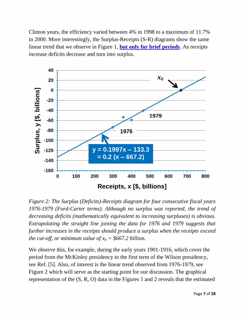
Figure 2: The Surplus (Deficits)-Receipts diagram for four consecutive fiscal years

1976-1979 (Ford-Carter terms). Although no surplus was reported, the trend of

decreasing deficits (mathematically equivalent to increasing surpluses) is obvious.

Extrapolating the straight line joining the data for 1976 and 1979 suggests that

further increases in the receipts should produce a surplus when the receipts exceed

the cut-off, or minimum value of x0 = $667.2 billion.

We observe this, for example, during the early years 1901-1916, which cover the

period from the McKinley presidency to the first term of the Wilson presidency,

see Ref. [5]. Also, of interest is the linear trend observed from 1976-1979, see

Figure 2 which will serve as the starting point for our discussion. The graphical

representation of the (S, R, O) data in the Figures 1 and 2 reveals that the estimated

-160

-140

-120

-100

-80

-60

-40

-20

0

20

40

0 100 200 300 400 500 600 700 800

Receipts, x [$, billions]

Su

rplu

s,

y [

$,

bil

lio

ns

]

1976

1979

y = 0.1997x – 133.3 = 0.2 (x – 667.2)

x0

Page 8 of 28

cut-off receipts x0 was $667.2 billion based on the US economy in 1976-1979 but

was up to $1616.93 billion in the 1994-2000 period.

We will now consider how this transition occurred using the S-R diagrams.

§ 3. The Surplus-Receipts Diagram for 1976-1984

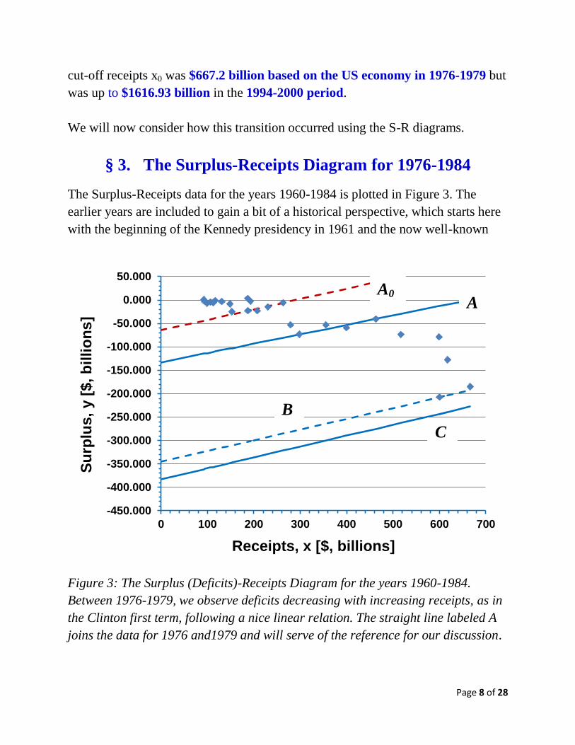
The Surplus-Receipts data for the years 1960-1984 is plotted in Figure 3. The

earlier years are included to gain a bit of a historical perspective, which starts here

with the beginning of the Kennedy presidency in 1961 and the now well-known

Figure 3: The Surplus (Deficits)-Receipts Diagram for the years 1960-1984.

Between 1976-1979, we observe deficits decreasing with increasing receipts, as in

the Clinton first term, following a nice linear relation. The straight line labeled A

joins the data for 1976 and1979 and will serve of the reference for our discussion.

-450.000

-400.000

-350.000

-300.000

-250.000

-200.000

-150.000

-100.000

-50.000

0.000

50.000

0 100 200 300 400 500 600 700

Receipts, x [$, billions]

Su

rplu

s,

y [

$,

bil

lio

ns

]

A A0

B

C

Page 9 of 28

Kennedy-Johnson tax cuts which are now widely believed to have invigorated the

economy (at least this is the opinion of those who believe in the benefits of such

tax cuts, see Refs. [11-22]). The straight line labeled A is our reference, and joins

the data for 1976 and1979, as in Figure 2.

Notice that the (S, R) data starts deviating from line A after 1979. Also, the data

for prior years is deviating from another line labeled A0 and approaches the line A.

What we witness here is like a transition between the parallels A0, A, and B.

Line A0 : y = 0.222x – 64.6 = 0.22 (x – 290.85) joining 1971 to 1974

Line A: y = 0.1997x – 133.3 = 0.20 (x – 667.2) joining 1976 and 1979

Line B: y = 0.229x – 345.3 = 0.23 (x - 1508.5) joining 1983 and 1987

Line C: y = 0.232x – 382.7 = 0.23 (x – 1648.8) joining 1985 and 1989

The equations of these lines were deduced from the actual (S, R) data. The Lines B

and C are indeed PERFECT parallels with identical slopes. The slopes of the other

lines differ only in the second decimal place. We see, therefore, a movement of the

data, or a cascading of the surplus, to lower and lower values (deficits increasing)

along these parallels even as the receipts increased year after year. More

importantly, this means that the cut-off revenue x0 varies as a function of time and

is NOT a constant. This is a complex system whose behavior we are trying to

understand using the simplest of all possible mathematical models.

Gerald Ford (seen receiving a kiss from his wife,

Betty) was the 40th vice president (1973-1974),

serving under President Richard Nixon. He was

appointed to the office after Agnew’s

resignation, the first person to be named vice

president under terms of the 25th Amendment.

Ford’s name at birth was Leslie King Jr. His

parents separated and he later took the name

of his mother’s second husband, although he

was never formally adopted.

http://img3.catalog.photos.msn.com/Image.aspx?uuid=5bcd672c-c35f-47e6-86e4-

1985453c4a96&w=628&h=498&so=2

Page 10 of 28

Figure 4: An expanded S-R diagram for the years 1960-1974 (Kennedy-Johnson to

Nixon-Ford) years.

Deficits also turned into a surplus moving along the line labeled B0, Figure 4, with

the equation y =0.119x – 19.02 – 0.12 (x -159.67), joining the 1962 and 1969 data

points. This is not a movement along parallels but the trend of “cascading” down to

higher deficit levels is similar. The solid blue dots are the cut-off receipts.

§ 4. The Surplus-Receipts Diagram for 1960-2001

The movement along parallels that is evident in Figure 3 (see also Figure 5 which

includes the data for subsequent years, through 2001) also has another and more

interesting implication and seems to provide empirical evidence for what might be

called the “economic” work function. This is analogous to the “work function” W

introduced in physics by Einstein, in 1905, to explain the puzzling (and equal

complex) phenomenon called photoelectricity. This has been discussed in Refs.[3-

-50.00

-40.00

-30.00

-20.00

-10.00

0.00

10.00

20.00

30.00

0.00 50.00 100.00 150.00 200.00 250.00 300.00 350.00

Receipts, x [$, billions]

Su

rplu

s,

y [

$,

bil

lio

ns

]

A0

x0

x0

y = 0.222x – 64.6 = 0.22 (x – 290.85)

B0

1967

1968

1969

1962

1960

Page 11 of 28

6] and the reader is referred to those articles. It is sufficient to note here that

Einstein’s photoelectric law, K = E – W = hf – W, is also a linear law which can be

written as y = hx + c = h(x – x0) where x is the frequency f, h the Planck constant

and hx = E the energy of a photon, y = K is the energy of the electron (produced

when light shines on the surface of a metal, light being a stream of photons all

having the energy hx), c is the negative of the work function W and x0 = -c/h = f0

= W/h is the cut-off frequency, the minimum frequency above which electrons are

produced (or a minimum photon energy W = hx0 = hf0 that must be exceeded).

Figure 5: The Surplus (Deficits)-Receipts Diagram for the years 1960-2001. Here

we consider the data going beyond 1984 all the way through the Clinton years. The

same three lines A, B, C are included here as in Figure 3.

Money in economics can be treated just like energy in physics (and vice versa) and

the above means that the US economy, at different times, is behaving like light

shining on different metals with different values of the work function W. Each

metal is different and has very different number of electrons in what is called the

-500

-400

-300

-200

-100

0

100

200

300

400

0 500 1000 1500 2000 2500

Receipts, x [$, billions]

Su

rplu

s,

y [

$,

bil

lio

ns

]

A

C

B

1985 1989

1981

1992

2000

2001

Page 12 of 28

valence shell. (We are using the simple model of the atom with a nucleus and

electrons in orbit in different “shells”, the outermost being the “valence” shell.)

How electrons are bound to the metal is therefore different and this changes the

work function W. The K-f graph for the photoelectric effect is a series of parallels

each having the slope h equal to the Planck constant and an intercept c = - W on

the y-axis and an intercept x = x0 = f0 on the x-axis.

It appears that we are witnessing similar changes here – the economic environment

is like the complex environment in which electrons exist in a metal. As it changes,

the economic work function changes and the system cascades down the parallels

until it meets another. The data for 1983 and 1984 indeed fall on or close to

parallel line B with the data for the intervening years representing a “transition”.

We also see the same type of a transition between the lines A0 and A. Recall that

the line A0 joins the data for 1971 and 1974. If the US economy had continued

along this line a surplus would have reported once the receipts exceeded the cut-off

x0 = $291 billion. The receipts for 1976, $298.060, were slightly in excess of this

cut-off. Alas, no surplus was observed! The explanation lies in the fact that the

“economic” work function had changed, i.e., x0 (the cut-off revenue) had increased

due to the changed economic environment.

Considering Figure 5, we see the data for 1983 and 1984 on the parallel B and the

data for 1985 and 1989 on the parallel C. Between 1981 and 1982, the national

debt crossed the trillion dollar, and so it is that President Reagan said on March 28,

1982, see Refs.[14-16], “We don’t have a trillion dollar debt because we haven’t

taxed enough. We have a trillion dollar debt because we are spending too much.”

Then, in 1989-1990, the annual receipts crossed the $1T mark, and now the annual

deficits have also crossed the $1T mark (in 2009).

It is also of interest to note that the cut-off revenue x0 deduced from the 1985 to

1989 data, the equation for Line C, equals $1648.8 billion. If the (S, R) data had

continued along line C, a surplus would be observed only when receipts exceeded

$1.65 trillion. In other words, the seeds for the debt-deficits problems that we are

witnessing today were sown a long time ago. (We can appreciate this further, from

the discussion to follow.)

Page 13 of 28

Instead of moving up the parallel C, the (S, R) data kept cascading down further

until we see a dramatic change in the slope starting with FY 1992. (One could

readily visualize straight lines with a negative connecting the data for the transition

years.) This marks the second half of the senior Bush term and the trend of both

increasing receipts with decreasing deficits continued through 2000. The slope of

the S-R line changed from a negative value to a positive value (see Figure 2 in Ref.

[3]) and a surplus was reported when the receipts exceeded $1616.93 billion.

Figure 6: The regression line for the Clinton years (1994-2000, labeled CL) is

added here. Because of the steeper positive slope h = 0.5845, this Clinton line

intersects the parallels A, B, C and crosses the x-axis (zero surplus or deficit) at a

point between the cut-off revenues deduced from lines B and C.

Quite interestingly, as illustrated graphically in Figure 6, the cut-off value observed

during the Clinton years ($1616.94 billion), when a surplus was finally reported,

falls between the cut-off values of $1508.5 billion and $1648.8 billion deduced by

extrapolation of the lines B and C.

-500

-400

-300

-200

-100

0

100

200

300

400

500

0 500 1000 1500 2000 2500

Receipts, x [$, billions]

Su

rplu

s,

y [

$,

bil

lio

ns

]

y= hx + c = h(x – x0) = 0.5845x – 945.04

= 0.5845 (x – 1616.93) r2 = 0.998

CL

Page 14 of 28

This is further proof of the observation made earlier that the “seeds of the

current debt-deficit problem that we are facing today were sown a long time

ago”. The following observations provide further confirmation.

1. As deficits changed to surplus, the (S, R) data following the Clinton line CL

rises to a peak value just shy of the extrapolation of line A, deduced from the

1971 and 1974 data (the Nixon years).

2. When the deficits were decreasing the (S, R) data fall on or close to the lines

B and C deduced from the 1980s data (Reagan-senior Bush).

3. When the receipts fell between 2000 and 2001 and the surplus decreased, the

(S, R) data again lies close the extrapolation suggested by Line B.

§ 5. Brief Discussion

The brief review of the (S, R, O) data, from 1960-2011, presented here (following

up on discussions in Refs.[3-6]), shows that the Clinton-years trend, of decreasing

deficits which turn into a surplus as receipts increase, has also been in earlier

periods but only briefly, example 1976-1979. Sometimes this is observed with data

for nonconsecutive years, although in chronological order (example the line B0 of

Figure 4, for 1962-1969, with 1967 and 1968 data falling below the line). The

implications of the remarkably linear Surplus-Receipts line, labeled as the Clinton

line (CL) was discussed earlier, Ref.[3], using the simple breakeven model for the

profitability of a company. We will consider this again here, to clarify the

implications of this linear trend further.

If we consider the operation of a company, with a profit motive, making and

selling N units of some products, all of the revenues of the company, “pN”, do not

appear as profits. Some of it must be given up, in the form of fixed costs, say “a”,

and the variable costs, say “bN”, associated with the operation of the company. It

is readily shown that the revenues x and the profits y, in this scenario, are related

by the linear law, y = hx + c = h(x – x0) where x0 = -c/h = ap/(p –b). The detailed

steps of the derivation may be found in Ref. [3]. Here “a” is the fixed cost, “b” the

unit variable cost, and “p” the unit price. A profit will appear only if the fixed cost

Page 15 of 28

“a” is exceeded. Even after the fixed costs are exceeded, only the portion (pN –

bN) of the additional revenues will appear as profits because of the variable costs.

Hence, profits appears at the breakeven x0 = ap/(p – b) > a. The intercept c = -a.

This is the intercept made on the y-axis (not of current interest). It is the intercept

made with the x-axis (the breakeven value x0) which is of interest to us here.

Fixed cost = a = -c, intercept on y-axis

Breakeven x0 = ap/(p –b) = a /[1 – (b/p)] = a/h > a since h < 1

Likewise, as government’s receipts increase, we expect the surplus to increase.

However, not all of the receipts will appear as a surplus. Some of the receipts must

be given up to meet the outlays, which are analogous to the costs of operation for a

company. The breakeven, or cut-off, receipts x0, also equals the maximum outlays

at any point in time. This cut-off receipts x0 has been going up consistently since

1901. For example, the breakeven estimated from the 1976-1979 data, when

deficits were being reported, was $667.2 billion. No surplus, however, appeared

when the receipts exceeded this level by 1985. A surplus was finally observed only

during the Clinton years. Deficits have reappeared since then. The transition to

higher and higher breakeven levels is illustrated here using the simple Surplus

(Deficits)-Receipts diagrams.

The “budget cuts” must first focus on the outlays that exceed the maximum x0,

just as we must distinguish between the bare minimum necessities of life and the

luxuries of life. This is the significant difference of the implications of the

constants “a” and “b” in the breakeven analysis for a simple company. Both are

related to costs, but in a very different manner.

To increase one’s savings (akin to the goal of producing a surplus) one has to focus

first on reducing the luxuries. One cannot focus on cutting the bare minimum

necessities that affect one’s standard of living. This would be like the misguided

focus on reducing the fixed cost “a” for a company, whereas a struggling company

must first focus its attention on reducing the unit variable cost “b”. The second step

would be to focus on reducing the fixed cost “a”. The same applies to the problem

improving the efficiency of the government by addressing the contentious,

divisive, but necessary, problem of budget cuts.

Page 16 of 28

The focus on cost-cutting by several global companies, with a focus on reducing

the head count/labor costs appears to be an example of focus on “a” as opposed to

“b” and this has, probably, led to the long term decline of many companies and

also the overall decline of the US economy. The Einstein and Henry Ford quotes

that follow are noteworthy in this context. The Reagan quote is also noteworthy

and serves as a reminder that government does have a role to play, especially in

times of a severe crisis; see also Greer, Ref.[18].

In summary, the linear law y = hx + c = h(x – x0) provides a simple and consistent

explanation for some of the key characteristics of the S-R diagrams used here to

analyze the Surplus-Receipts data. The intercept x0 = -c/h has the characteristics of

the “breakeven costs”, or the cut-off photon energy in Einstein’s photoelectric law.

The nonzero intercept c in the linear law can thus be treated as the “economic”

work function. The changes in this economic work function, as a function of time,

have been discussed here and can be used as a tool to learn how to “design” a

budget that will yield a surplus year after year.

To use the analogy of heat engines, many companies, and the economy, today are

operating “erratically” like the old Newcomen steam engines, before James Watt

began his studies that led to a permanent improvement in the performance of steam

engines. Furthermore, as shown in the companion article (Ref.[3]) a review of all

the (S, R, O) data going back to 1901 shows that the “Government Engine”,

although working erratically, does have the potential to operating with an

efficiency E = S/R in the range of 20% to 30%, which is comparable to the thermal

efficiency of modern, finely tuned, engines. Typically, only a third of the heat

energy released by burning of the fuel in the engine appears as useful work.

Likewise, the government economists and political leaders, from the President

down, who are in charge of formulating the annual budget, must learn to focus on

understanding how to make the “Government Engine” work in a consistent

manner, to launch a new era of “financial efficiency” in government.

Page 17 of 28

Some Quotes to Ponder in the Modern Context

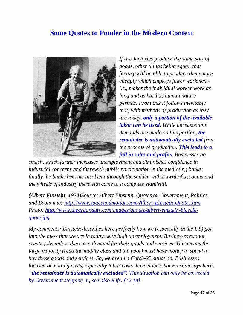
If two factories produce the same sort of

goods, other things being equal, that

factory will be able to produce them more

cheaply which employs fewer workmen -

i.e., makes the individual worker work as

long and as hard as human nature

permits. From this it follows inevitably

that, with methods of production as they

are today, only a portion of the available

labor can be used. While unreasonable

demands are made on this portion, the

remainder is automatically excluded from

the process of production. This leads to a

fall in sales and profits. Businesses go

smash, which further increases unemployment and diminishes confidence in

industrial concerns and therewith public participation in the mediating banks;

finally the banks become insolvent through the sudden withdrawal of accounts and

the wheels of industry therewith come to a complete standstill.

(Albert Einstein, 1934)Source: Albert Einstein, Quotes on Government, Politics,

and Economics http://www.spaceandmotion.com/Albert-Einstein-Quotes.htm

Photo: http://www.theargonauts.com/images/quotes/albert-einstein-bicycle-

quote.jpg

My comments: Einstein describes here perfectly how we (especially in the US) got

into the mess that we are in today, with high unemployment. Businesses cannot

create jobs unless there is a demand for their goods and services. This means the

large majority (read the middle class and the poor) must have money to spend to

buy these goods and services. So, we are in a Catch-22 situation. Businesses,

focused on cutting costs, especially labor costs, have done what Einstein says here,

“the remainder is automatically excluded”. This situation can only be corrected

by Government stepping in; see also Refs. [12,18].

Page 18 of 28

“The Federal Government should only do what the people cannot do for

themselves or through their locally elected leaders.”

- President Ronald Reagan, Address Before a Joint Session of the Alabama State

Legislature in Montgomery, March 15, 1982.

Source: http://www.freerepublic.com/focus/news/838536/posts See under

Government.

“Nearly everything in this country is too

high priced. The only thing that should be

high priced in this country is the man that

works. Wages must not come down, they

must not even stay on their present level;

they must go up. And even that is not

sufficient of itself -- we must see to it that

the increased wages are not taken away

from the people by increased prices that do

not represent increased values.”

Henry Ford, New York Times, November

22, 1929 (5.0% unemployment)

Source: http://www.friesian.com/sayslaw.htm

Photo: http://s1.aecdn.com/images/news/legacy-of-the-ford-model-t-100-years-

after-1380_2.jpg

It is often overlooked that, going beyond the well-known innovations in

automobile manufacturing that he introduced, Henry Ford did FOUR remarkable

things: a) increased the wages of his employees, b) increased the demand for his

Model T c) decreased prices and d) increased the revenues and the profits of Ford

Motor Company.

“I am convinced that the larger incomes of the country would actually yield more

revenue to the government if the basis of taxation were scientifically revised

downward.”

President Calvin Coolidge, State of the Union message, December 3, 1924.

Page 19 of 28

§ 7. List of References

1. Fiscal Year 2013 Budget of the US Government,

http://www.whitehouse.gov/sites/default/files/omb/budget/fy2013/assets/hist.pdf

2. Bill Clinton Speech at the Democratic National Convention: GOP ‘Built’

the National Debt, Amanda Terkel, aterkel@huffingtonpost.com, Sep 4, 2012,

http://www.whitehouse.gov/sites/default/files/omb/budget/fy2013/assets/hist.pdf

3. The Efficiency of Government Compared to the Thermal Efficiency of a

Heat Engine, Sep 18, 2012, http://www.scribd.com/doc/106220758/The-

Efficency-of-Government-Compared-to-Thermal-Efficiency-of-a-Heat-Engine

4. The Amazing US Government Surplus (Deficits)-Receipts Relation during

the Clinton Presidency, http://www.scribd.com/doc/105821230/The-Amazing-

US-Government-Receipts-Surplus-Relation-during-the-Clinton-Presidency,

Published Sep 13, 2012.

5. A Brief Review of the Historical US Government Receipts-Surplus (Deficit)

Relation, http://www.scribd.com/doc/106003088/A-Brief-Review-of-the-

Historical-US-Government-Surplus-Receipts-Relation , Published Sep 15,

2012.

6. The Clinton Budget Surpluses, http://www.scribd.com/doc/105819500/The-

Clinton-Budget-Surpluses-Treating-Government-like-a-Business, Published

Sep 13, 2012 , Google financial data for early years may be found in Table 2.

7. From Debt-free to $16T: Lessons to be learned, Sep 11, 2012, scribd.com,

http://www.scribd.com/doc/105651734/From-Debt-Free-to-16T-Lessons-to-be-

learned

8. The US National Debt Growth Rate: The Clinton-Bush-Obama

Transitions, Sep 6, 2012. www.scribd.com <

http://www.scribd.com/doc/105058946/The-US-National-Debt-Growth-Rate-

The-Clinton-Bush-Obama-Transition >

9. The Rate of Growth of the National Debt: The Obama versus Bush years,

Sep 4, 2012. www.scribd.com < http://www.scribd.com/doc/104803209/The-

Rate-of-Growth-of-the-National-Debt-The-Obama-versus-the-Bush-years >

10. Is Taxing the Rich an Option for Budget Deficit Reduction?, Sep 2, 2012.

www.scribd.com < http://www.scribd.com/doc/104661297/Is-Taxing-the-Rich-

an-Option-for-Budget-Deficit-Reduction

Page 20 of 28

11. Two of the All-Time Greatest Successes in Cutting Taxes and Spending, by

Jim Powell, forbes.com, August 10, 2011

http://www.forbes.com/sites/realspin/2011/08/10/two-of-the-all-time-greatest-

successes-in-cutting-taxes-and-spending/

12. Econ 101: How do Tax Cuts Work? By Gary Wolfram, Nov 11, 2006,

mrc.org, http://www.mrc.org/node/29589

13. Success of Tax Cuts, By John R. Hendrickson, Oct 2006, insideronline.org,

http://www.insideronline.org/archives/2007/winter/chap7.pdf

14. Contemporary Quotes on Are Tax Cuts Good for the Economy? Intellectual

takout.org, http://www.intellectualtakeout.org/content/contemporary-quotes-

are-tax-cuts-good-economy

15. Quotes – Ronal Reagan, March 28, 1982 fightthebias.com

http://www.fightthebias.com/quotes/ronald_reagan.htm

16. It’s Not a Revenue Problem, it’s a Spending Problem, Tracing the history of

a GOP talking point, David Weigel, April 18, 2011, slate.com,

http://www.slate.com/articles/news_and_politics/politics/2011/04/its_not_a_rev

enue_problem_its_a_spending_problem.html

17. GOP on Message, Revenue Not the Problem, Spending Is, foxnews.com,

Nov 7, 2010, http://www.foxnews.com/politics/2010/11/07/gop-message-

revenue-problem-spending/

18. The Biggest Engine of Economic Growth?, By Colin Greer, newwf.org,

March 19, 2012, http://newwf.org/blog/2012-03-19-the-biggest-engine-of-

economic-growth

19. Laffer Curve, http://www.investopedia.com/terms/l/laffercurve.asp

20. Arthur Laffer’s Ant-Stimulus Curve Ball is a Foul, David Futrelle, August

9, 2012, business.time.com, http://business.time.com/2012/08/09/arthur-laffers-

anti-stimulus-curve-ball-is-a-foul/

21. The Laffer Curve in the 1980s, by Mark J. Perry, mjperry.blogspot.com, Jan

26, 2008, http://mjperry.blogspot.com/2008/01/laffer-curve-in-1980s.html

22. The Laffer Curve, http://en.wikipedia.org/wiki/Laffer_curve

23. Sixteenth Amendment to the United States Constitution, Wikipedia article,

http://en.wikipedia.org/wiki/Sixteenth_Amendment_to_the_United_States_Con

stitution http://www.shmoop.com/constitution/16th-amendment.html

24. Woodrow Wilson, Congress and the Income Tax, March 16, 2004,

wilsoncenter.org http://www.wilsoncenter.org/sites/default/files/ACF18.pdf

Page 21 of 28

25. The Effect of Hikes and Cuts in the Tax Rates on Government Receipts in

the Wilson-Harding-Coolidge terms, To be Published.

26. The Question Is: Will we be better off in four years?, Robert Samuelson,

http://www.dispatch.com/content/stories/editorials/2012/09/10/the-question-is-

will-we-be-better-off-in-four-years.html

***********************************************************

§ 8. Appendix I

Bibliography of Related Articles

Posted at this website Since Facebook IPO on May 18, 2012

The first article listed below discusses a little known mathematical property of a

straight line. Figures 1 to 3 in this article provide the philosophical basis for

considering the significance of a nonzero intercept c as it applies to many problems

in the real world. We make observations (x and y values of interest to us) to deduce

y/x, usually called “rates”, “ratios”, or percentages.

1. http://www.scribd.com/doc/102000311/A-Little-Known-Mathematical-

Property-of-a-Straight-Line-Strange-but-true-there-is-one Published August 4,

2012.

Financial data (Profits-Revenues) analysis and Generalization of Planck’s law

beyond physics.

2. http://www.scribd.com/doc/95906902/Simple-Mathematical-Laws-Govern-

Corporate-Financial-Behavior-A-Brief-Compilation-of-Profits-Revenues-

Data Current article with all others above cited for completeness, Published

June 4, 2012 with several revisions incorporating more examples.

3. http://www.scribd.com/doc/94647467/Three-Types-of-Companies-From-

Quantum-Physics-to-Economics Basic discussion of three types of

companies, Published May 24, 2012. Examples of Google, Facebook,

ExxonMobil, Best Buy, Ford, Universal Insurance Holdings

Page 22 of 28

4. http://www.scribd.com/doc/96228131/The-Perfect-Apple-How-it-can-be-

destroyed Detailed discussion of Apple Inc. data. Published June 7, 2012.

5. http://www.scribd.com/doc/95140101/Ford-Motor-Company-Data-Reveals-

Mount-Profit Ford Motor Company graph illustrating pronounced maximum

point, Published May 29, 2012.

6. http://www.scribd.com/doc/95329905/Planck-s-Blackbody-Radiation-Law-

Rederived-for-more-General-Case Generalization of Planck’s law,

Published May 30, 2012.

7. http://www.scribd.com/doc/94325593/The-Future-of-Facebook-I Facebook

and Google data are compared here. Published May 21, 2012.

8. http://www.scribd.com/doc/94103265/The-FaceBook-Future Published May

19, 2012 (the day after IPO launch on Friday May 18, 2012).

9. http://www.scribd.com/doc/95728457/What-is-Entropy Discussion of the

meaning of entropy (using example given by Boltzmann in 1877, later also

used by Planck to develop quantum physics in 1900). The example here shows

the concepts of entropy S and energy U (and the derivative T = dU/dS) can be

extended beyond physics with energy = money, or any property of interest.

Published June 3, 2012.

10. The Future of Southwest Airlines, Completed June 14, 2012 (to be

published). http://www.scribd.com/doc/102835946/The-Future-for-Southwest-

Airlines-The-Unknown-Story-of-Rising-Costs-and-the-Maximum-Point-on-

Profits-Revenues-Curve Published August 14, 2012.

11. The Air Tran Story: An Important Link to the Future of Southwest Airlines,

Completed June 27, 2012 (to be published).

http://www.scribd.com/doc/102832984/The-Air-Tran-Story-The-Merger-and-

Maximum-Point-on-Profits-Revenues-Graph Published August 14, 2012.

12. Annie’s Inc. A Single-Product Company Analyzed using a New

Methodology, http://www.scribd.com/doc/98652561/Annie-s-Inc-A-Single-

Product-Company-Analyzed-Using-a-New-Methodology Published June 29,

2012

Page 23 of 28

13. Google Inc. A Lovable One-Trick Pony Another Single-product Company

Analyzed using the New Methodology.

http://www.scribd.com/doc/98825141/Google-A-Lovable-One-Trick-Pony-

Another-Single-Product-Company-Analyzed-Using-the-New-Methodology,

Published July 1, 2012.

14. GT Advanced Technologies, Inc. Analysis of Recent Financial Data,

Completed on July 4, 2012. (To be published).

15. Disappearing Brands: Research in Motion Limited. An Interesting type of

Maximum Point on the Profits-Revenues Graph

http://www.scribd.com/doc/99181402/Research-in-Motion-RIM-Limited-Will-

Disappear-in-2013 Published July 5, 2012.

16. Kia Motor Company: A Disappearing Brand

http://www.scribd.com/doc/99333764/Kia-Motor-Company-A-Disppearing-

Brand, Published July 6, 2012.

17. The Perfect Apple-II: Taking A Second Bite: A Simple Methodology for

Revenues Predictions (Completed July 8, 2012, To be Published)

http://www.scribd.com/doc/101503988/The-Perfect-Apple-II, Published

July 30, 2012.

18. http://www.scribd.com/doc/101062823/A-Fresh-Look-at-Microsoft-After-its-

Historic-Quarterly-Loss Microsoft after the quarterly loss, Published July 25,

2012.

19. http://www.scribd.com/doc/101518117/A-Second-Look-at-Microsoft-After-the-

Historic-Quarterly-Loss , Published July 30, 2012.

20. http://www.scribd.com/doc/103265909/A-Brief-Analysis-of-Groupon-s-Profits-

Revenues-Data Published August 19, 2012.

21. http://www.scribd.com/doc/103027366/Groupon-Analysis-of-Profits-

Revenues-Data-and-its-Business-Model Published August 16, 2012. More

detailed analysis including discussion of the idea of a work function.

22. http://www.scribd.com/doc/103369016/Analysis-of-Zynga-s-Profits-Revenues-

Data-Maximum-point-on-the-profits-revenues-curve Published August 20,

2012.

Page 24 of 28

General Motors Financial Data

23. http://www.scribd.com/doc/103600274/The-New-GM-A-Brief-Analysis-of-the-

Profits-Revenues-Data-through-1Q2011, Published May 9, 2011 and again on

August 22, 2012, Discussion of the new GM data from 1Q2010 to 1Q2011.

24. http://www.scribd.com/doc/103607023/Why-Can-t-General-Motors-be-more-

like-Microsoft-The-new-GM-may-just-be Published August 22, 2012.

25. http://www.scribd.com/doc/103938349/GM-Before-the-Bankruptcy-Maximum-

Point-on-Profits-Revenue-Graph GM Before the Bankruptcy: Maximum

point on the profits-revenues graph, Published August 25, 2012.

******************************************************************

The Unemployment Problem: Evidence for a Universal value of h in the

unemployment law.

26. http://www.scribd.com/doc/100984613/Further-Empirical-Evidence-for-the-

Universal-Constant-h-and-the-Economic-Work-Function-Analysis-of-

Historical-Unemployment-data-for-Japan-1953-2011 Single universal value of

h for US, Canada and Japan in the unemployment law y = hx + c, Published

July 24, 2012.

27. http://www.scribd.com/doc/100939758/An-Economy-Under-Stress-

Preliminary-Analysis-of-Historical-Unemployment-Data-for-Japan, Published

July 24, 2012.

28. http://www.scribd.com/doc/100910302/Further-Evidence-for-a-Universal-

Constant-h-and-the-Economic-Work-Function-Analysis-of-US-1941-2011-and-

Canadian-1976-2011-Unemployment-Data Published July 24, 2012.

29. http://www.scribd.com/doc/100720086/A-Second-Look-at-Australian-2012-

Unemployment-Data, Published July 22, 2012.

30. http://www.scribd.com/doc/100500017/A-First-Look-at-Australian-

Unemployment-Statistics-A-New-Methodology-for-Analyzing-Unemployment-

Data , Published July 19, 2012.

31. http://www.scribd.com/doc/99857981/The-Highest-US-Unemployment-Rates-

Obama-years-compared-with-historic-highs-in-Unemployment-levels ,

Published July 12, 2012.

32. http://www.scribd.com/doc/99647215/The-US-Unemployment-Rate-What-

happened-in-the-Obama-years , Published July 10, 2012.

****************************************************************

Page 25 of 28

Traffic-fatality and Teen pregnancy problem

33. http://www.scribd.com/doc/101982715/Does-Speed-Kill-Forgotten-US-

Highway-Deaths-in-1950s-and-1960s Published August 4, 2012.

34. http://www.scribd.com/doc/101983375/Effect-of-Speed-Limits-on-Fatalities-

Texas-Proofing-of-Vehciles Published August 4, 2012.

35. http://www.scribd.com/doc/101828233/The-US-Teenage-Pregnancy-Rates-1

Published August 2, 2012.

36. http://www.scribd.com/doc/102384514/A-Second-Look-at-the-US-Teenage-

Pregnancy-Rates-Evidence-for-a-Predominant-Natural-Law Published August

8, 2012.

Government and National Debt

37. http://www.scribd.com/doc/104663110/The-United-States-Postal-Service-A-

Test-Case-to-Understand-the-US-Government-Inefficiencies-and-Budget-Cuts-

Ahead United States Postal Service: A Test case for government inefficiencies,

Published Sep 2, 2012.

38. http://www.scribd.com/doc/104833993/Are-You-Better-Off-Than-You-Were-

Four-Years-Ago Published Sep 4, 2012. Briefly highlights the slowing down

the debt growth rate as we cross the $16 T mark. The national debt could have

been as high as $19.5T on August 30, 2012 if the high rate at the end of the

Bush presidency had continued.

39. http://www.scribd.com/doc/104803209/The-Rate-of-Growth-of-the-National-

Debt-The-Obama-versus-the-Bush-years Published Sep 3, 2012. The

importance of the debt growth rate h = dD/dt, as opposed to the debt level D, is

emphasized. The significance of the debt growth rate does not seem to have

been recognized, at least in the popular discussion.

40. http://www.scribd.com/doc/104677653/The-US-National-Debt-Brief-History-

Good-News-The-Rate-of-Growth-of-the-Debt-is-Slowing-Down , Published

Sep 1, 2012. Brief summary of the historical debt data starting with President

George Washington with attention being drawn to the recent slowing down of

the debt growth rate. The importance of the debt growth rate, as opposed to debt

levels, does not seem to have been recognized, at least in the popular

discussion.

Page 26 of 28

41. http://www.scribd.com/doc/104659108/The-US-National-Debt-and-the-Long-

Term, first published on June 17, 2011, and republished Sep 1, 2012.

42. http://www.scribd.com/doc/104659448/The-US-National-Debt-Retirement-

Program, first published on June 23, 2011, before the debt default crisis which

led to lowering of the US rating, republished Sep 1, 2012.

43. http://www.scribd.com/doc/104662291/A-Radical-Proposal-to-Permanently-

Reduce-the-Unemployment-Rate, first published on October 13, 2011,

republished Sep 1, 2012.

44. http://www.scribd.com/doc/104661297/Is-Taxing-the-Rich-an-Option-for-

Budget-Deficit-Reduction, first published on July 3, 2011, republished Sep 1,

2012.

Page 27 of 28

About the author

V. Laxmanan, Sc. D.

Email: vlaxmanan@hotmail.com

The author obtained his Bachelor’s degree (B. E.) in Mechanical Engineering from

the University of Poona and his Master’s degree (M. E.), also in Mechanical

Engineering, from the Indian Institute of Science, Bangalore, followed by a

Master’s (S. M.) and Doctoral (Sc. D.) degrees in Materials Engineering from the

Massachusetts Institute of Technology, Cambridge, MA, USA. He then spent his

entire professional career at leading US research institutions (MIT, Allied

Chemical Corporate R & D, now part of Honeywell, NASA, Case Western Reserve

University (CWRU), and General Motors Research and Development Center in

Warren, MI). He holds four patents in materials processing, has co-authored two

books and published several scientific papers in leading peer-reviewed

international journals. His expertise includes developing simple mathematical

models to explain the behavior of complex systems.

While at NASA and CWRU, he was responsible for developing material processing

experiments to be performed aboard the space shuttle and developed a simple

mathematical model to explain the growth Christmas-tree, or snowflake, like

structures (called dendrites) widely observed in many types of liquid-to-solid phase

transformations (e.g., freezing of all commercial metals and alloys, freezing of

water, and, yes, production of snowflakes!). This led to a simple model to explain

the growth of dendritic structures in both the ground-based experiments and in the

space shuttle experiments.

More recently, he has been interested in the analysis of the large volumes of data

from financial and economic systems and has developed what may be called the

Quantum Business Model (QBM). This extends (to financial and economic

systems) the mathematical arguments used by Max Planck to develop quantum

physics using the analogy Energy = Money, i.e., energy in physics is like money in

economics. Einstein applied Planck’s ideas to describe the photoelectric effect (by

treating light as being composed of particles called photons, each with the fixed

quantum of energy conceived by Planck). The mathematical law deduced by

Page 28 of 28

Planck, referred to here as the generalized power-exponential law, might actually

have many applications far beyond blackbody radiation studies where it was first

conceived.

Einstein’s photoelectric law is a simple linear law, as we see here, and was

deduced from Planck’s non-linear law for describing blackbody radiation. It

appears that financial and economic systems can be modeled using a similar

approach. Finance, business, economics and management sciences now essentially

seem to operate like astronomy and physics before the advent of Kepler and

Newton.

Cover page of AirTran 2000 Annual