predicting regional crop production: applicationsjhansen/jones16july.pdfgeorgia soybean yield...

Predicting Regional Crop Production: Applications

James W. JonesUniversity of Florida

Questions

• Can models successfully predict variations in crop yield due to climate variations over time in a region in which soils, weather, and management vary?

• If so, how can they best be used?

• What are the requirements for this approach?

• Are there examples?

ObjectiveEvaluate approaches for predicting crop yield response to

climate variations, regional scale, using crop models

Hypotheses:

• 1. Use of local data is necessary for accurately predicting yield

• 2. Yield predictions are improved when local yield data are used to adjust estimates of soil properties relative to using general soil inputs

Irmak, Jagtap and Jones. 2002. (In Preparation)

Material and Methods• Region: Tift County, GA• Data:

– 24 years of county yield data. • 17 years for calibration• 7 years for independent validation (randomly selected)

– Yields were de-trended– 0.5 degree soils & weather data from VEMAP database

• Management: Rainfed practices based on NASS data, surveys• Simulations: Average of 9 planting dates, 3 varieties to account

for within county variations• Compare root mean square errors of prediction (independent

data)


Case 1: Base Case, no parameter estimation

• RMSEP = root mean square error for county j• Where m = # of validation years• Yij = Observed yield (kg/ha) for county j, year i• yij = Simulated yield (kg/ha) for county j, year i• j = county• i = year

∑ =−=

m

i ijij yYm

RMSEP1

2)(1


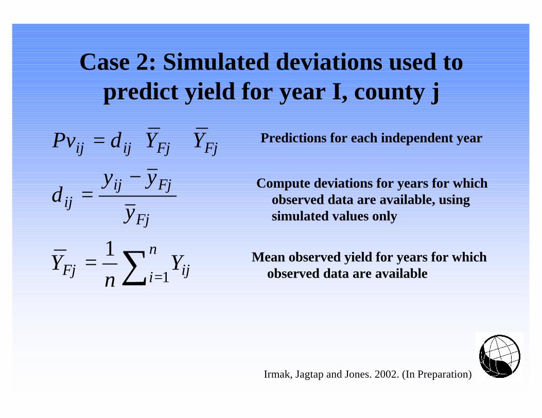
Case 2: Simulated deviations used to predict yield for year I, county j

1

1∑ ==

−=

+⋅=

n

i ijFj

Fj

Fjijij

FjFjijij

Yn

Y

y

yyd

YYdPv Predictions for each independent year

Compute deviations for years for which observed data are available, using simulated values only

Mean observed yield for years for which observed data are available


Case 3: Regression model adjustment of simulated values to account for bias (systematic and non-

systematic)

jk

jkjkijjij bVcyaPv +⋅+= ∑)(

Fitted yield using F dataset

Simulated yield for validation dataset

)(ˆ jk

jkjkijjij bVcyay +⋅+= ∑

• Where aj, bj, cjk = regression coefficients

• Vjk = k variables such as rainfall at planting, and rainfall at harvest


Case 4: Yield correction factor to account for average bias

)( ijij yYcfPv =

Yield Correction Factor = Observed/Simulated

Simulated yield for validation dataset

ij

ij

y

YYcf =

• Where yij = Simulated yield for grid j, year i

• Yij = Observed yield for grid j, year i


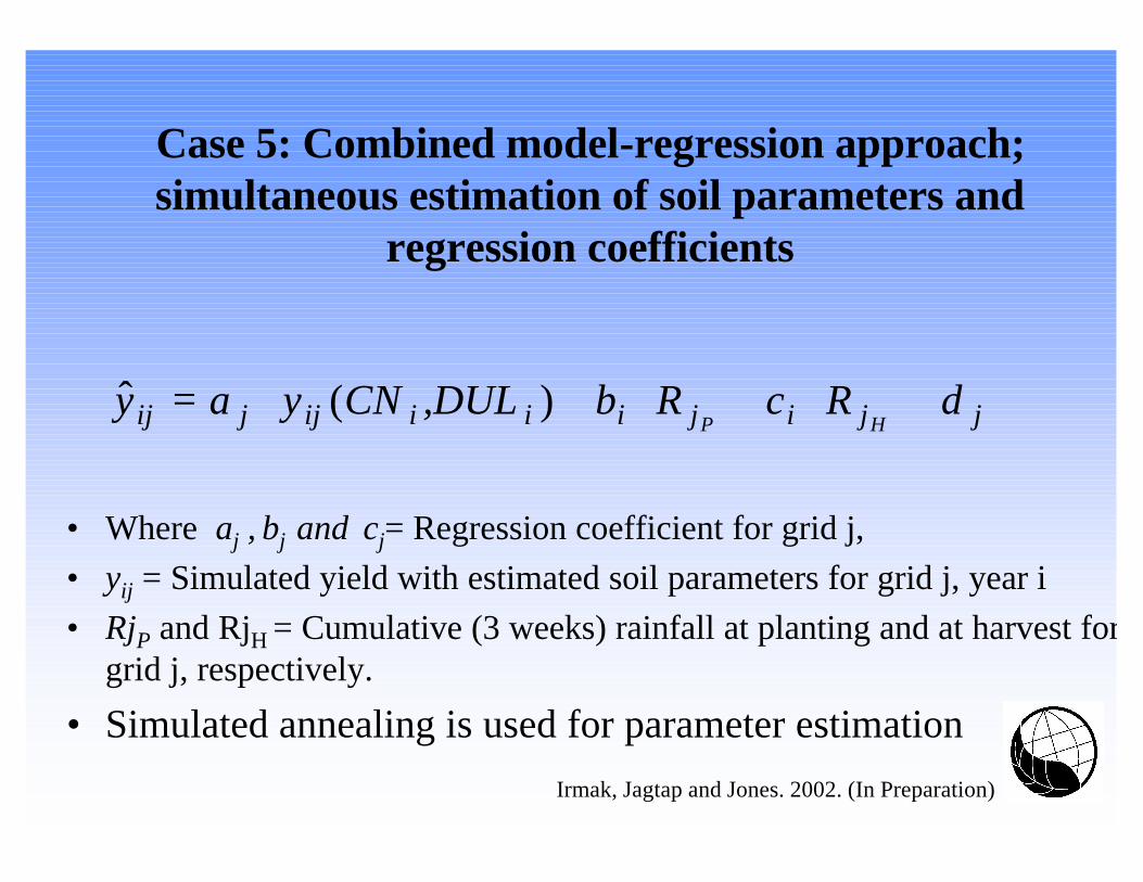
Case 5: Combined model-regression approach; simultaneous estimation of soil parameters and

regression coefficients

)(ˆ jjijiiiijjij dRcRb,DULCNyayHP

+⋅+⋅+⋅=

• Where aj , bj and cj= Regression coefficient for grid j,

• yij = Simulated yield with estimated soil parameters for grid j, year i

• RjP and RjH = Cumulative (3 weeks) rainfall at planting and at harvest for grid j, respectively.

• Simulated annealing is used for parameter estimation


Case 1, base case

0

500

1000

1500

2000

2500

3000

3500

4000

1972 1974 1976 1978 1980 1982 1984 1986 1988 1990 1992 1994

Year

Yie

ld (

kg

/ha

)

M S


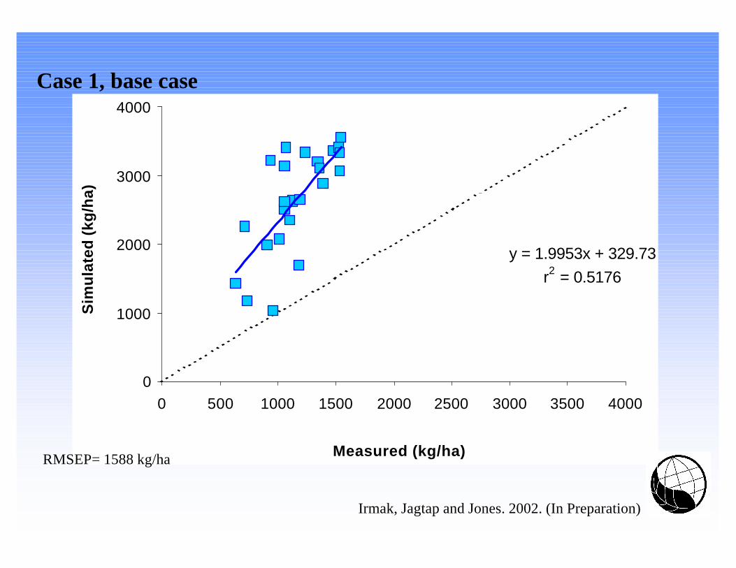
Case 1, base case

y = 1.9953x + 329.73

r2 = 0.5176

0

1000

2000

3000

4000

0 500 1000 1500 2000 2500 3000 3500 4000

Measured (kg/ha)

Sim

ula

ted

(kg

/ha)

RMSEP= 1588 kg/ha


Calibration

0

200

400

600

800

1000

1200

1400

1600

1800

1973 1976 1979 1982 1984 1987 1990 1992 1995

Year

Yie

ld (

kg/h

a)

M S

Case 2, Simulate deviations

Validation

0

500

1000

1500

2000

1972 1974 1977 1981 1986 1989 1994

Year

Yie

ld (k

g/h

a)

M

SRMSEvalidation = 348 kg/ha

RMSEfitting = 164 kg/ha


Calibrationy = 0.9432x + 64.251

r2 = 0.7062

Validationy = 0.6611x + 514.4

r2 = 0.2062

0

500

1000

1500

2000

2500

0 500 1000 1500 2000 2500

Measured (kg/ha)

Sim

ula

ted

(kg

/ha)

Calibration

Validation

Case 2:


Calibration

0

500

1000

1500

2000

1973 1976 1979 1982 1984 1987 1990 1992 1995

Year

Yie

ld (

kg/h

a)

M S

Validation

0

500

1000

1500

2000

1972 1974 1977 1981 1986 1989 1994

Year

Yie

ld (

kg/h

a)

M S

RMSEfitting = 167 kg/ha

Case 5, Estimate crop model And regression parameters

RMSEvalidation = 269 kg/ha


Validationy = 1.1034x + 34.366

r2 = 0.6186

Calibrationy = 1.0645x - 127.96

r2 = 0.7681

0

500

1000

1500

2000

2500

0 500 1000 1500 2000 2500

Measured (kg/ha)

Sim

ula

ted

(kg

/ha)

calibration

validation

1:1 line

Case 5:


Preliminary Conclusions

• Variations in yield associated with climate variations over time can be estimated with accuracies on the order of 5-10%

• Use of simulated deviations and historical yields to predict yield variations is a good first approximation (errors on the order of 10-20%)

• Availability of historical yields for an area can improve predictions, reducing errors by half or more


What is Required?

• Soil profile inputs, each grid or polygon

• Daily weather data, each grid or polygon

• Management inputs, each grid or polygon

• Crop model, evaluated using experiment station data for some location(s) in region

And, if available:

• Historical yield data for a number of years

Example for Georgia, USA

• Soybean study by Jagtap et al.

• 18 years of historical yield data (NASS database)

• Daily weather data provided at 50 km grid (VEMAP data base developed by NCAR)

• Dominant soil(s) for each 50x50 km grid cell (VEMAP)

• Management practices (NASS database & state Extension Specialists)

Georgia Soybean Yield Predictions

Jagtap and Jones, 2002, Agr. Ecosystems & Env.

Experience in applying current crop growth models to predict regional productions and its variability is limited.

A number of challenges arise when applying dynamic crop models to regional scales.

The interest is now increasing to use models more and more for policy and decision making at regional scales that are relevant to farmers, grain traders and other decision makers



Known are…

üHistorical county yields

ü50-km digital soil and weather data base

ü<7% of area cultivated

Unknown are..

Spatial variability in

Inputs

outputs



@ Plot level•Soil•Plant Population•Variety•Inputs•Weather

@ Field/Regional•Input Variations•Crop Regions•Planting Calendar•Weather



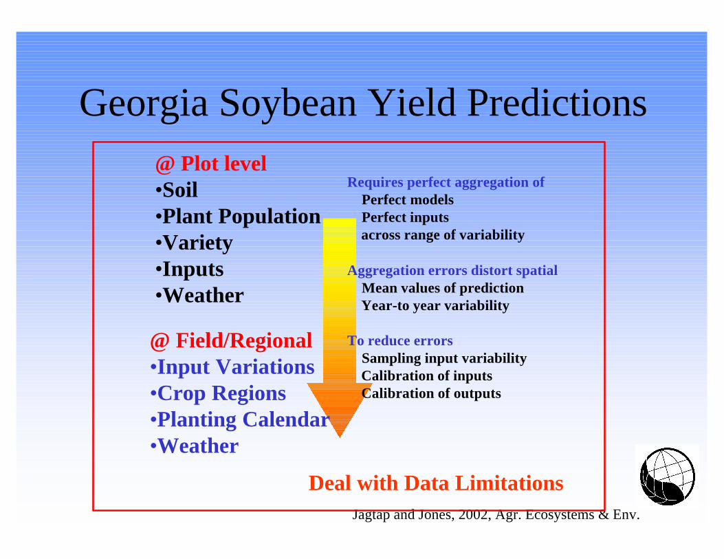
@ Plot level•Soil•Plant Population•Variety•Inputs•Weather

@ Field/Regional•Input Variations•Crop Regions•Planting Calendar•Weather

Requires perfect aggregation ofPerfect modelsPerfect inputsacross range of variability

Aggregation errors distort spatialMean values of predictionYear-to year variability

To reduce errorsSampling input variability Calibration of inputsCalibration of outputs

Deal with Data Limitations

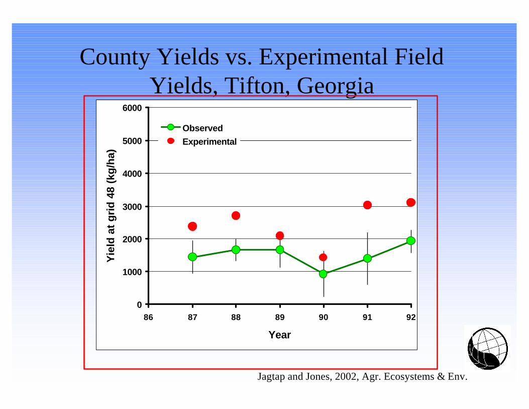
County Yields vs. Experimental Field Yields, Tifton, Georgia


0

1000

2000

3000

4000

5000

6000

86 87 88 89 90 91 92

Year

Yie

ld a

t g

rid

48

(kg

/ha)

Observed

Experimental

Crop Models Simulate Yield at Field Scale:Bias Exists


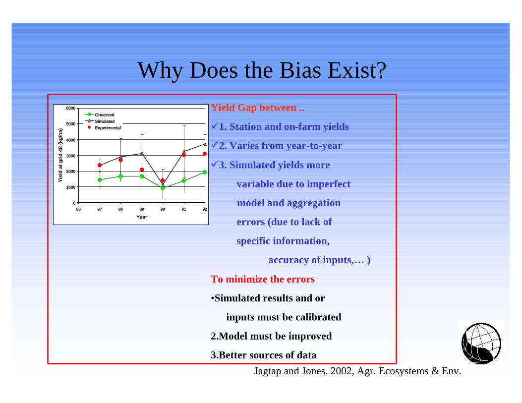
Why Does the Bias Exist?


0

1000

2000

3000

4000

5000

6000

86 87 88 89 90 91 92

Year

Yie

ld a

t g

rid

48

(kg

/ha)

Observed

SimulatedExperimental

Yield Gap between ..

ü1. Station and on-farm yields

ü2. Varies from year-to-year

ü3. Simulated yields more

variable due to imperfect

model and aggregation

errors (due to lack of

specific information,

accuracy of inputs,… )

To minimize the errors

•Simulated results and or

inputs must be calibrated

2.Model must be improved

3.Better sources of data

Unadjusted Crop Model Results


RMSE ranged from 0.24 to 0.65 t/ha or 16 to 47% of grid yields.RMSE during validation was 38-60% of the 1990-95 mean yields

0

1000

2000

3000

4000

5000

6000

70 75 80 85 90 95

Year

Yie

ld (

kg

/ha

)

ActualUn-Calibrated

Before Removing Bias, High RMSE for Validation Sites


Area lost in 1993<10%11 - 25 %>25%

N40 0 4 0 80 K ilo m eter s

RMSE 1993<20%21 - 40 % 41-60 %>60 %

N4 0 0 4 0 80 K ilo m ete rs

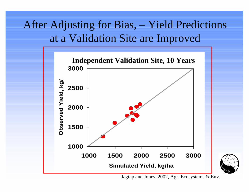
After Adjusting for Bias, – Yield Predictions at a Validation Site are Improved

1000

1500

2000

2500

3000

1000 1500 2000 2500 3000

Simulated Yield, kg/ha

Ob

serv

ed

Yie

ld, kg

/ha


Independent Validation Site, 10 Years

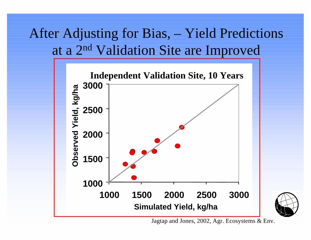
After Adjusting for Bias, – Yield Predictions at a 2nd Validation Site are Improved

1000

1500

2000

2500

3000

1000 1500 2000 2500 3000Simulated Yield, kg/ha

Ob

serv

ed Y

ield

, kg

/ha


Independent Validation Site, 10 Years

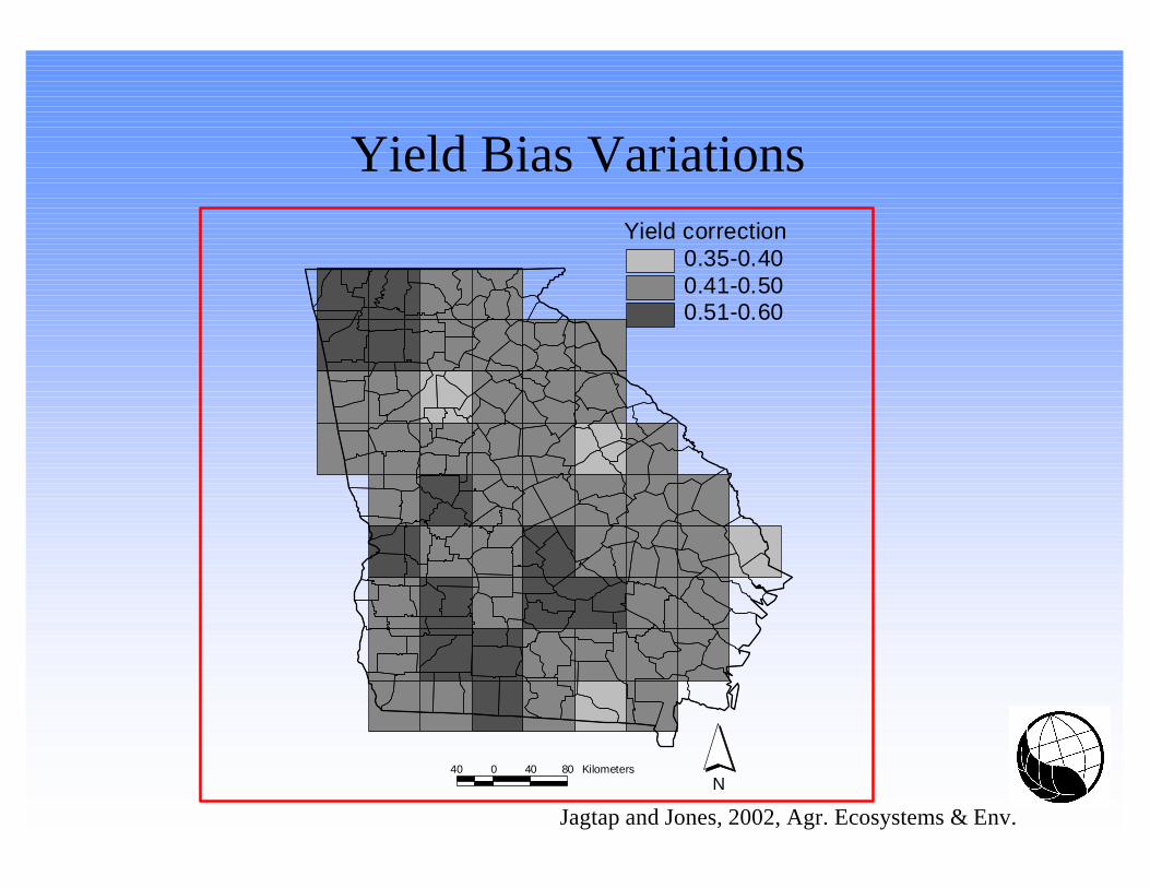
Yield Bias Variations


Yield correction0.35-0.400.41-0.500.51-0.60

N40 0 40 80 Kilometers

After Adjusting for Bias, RMSE for Independent Years Improved Greatly


RMSE<5 %6 - 10 %11 - 16 %

N40 0 40 80 Kilometers


0.0

0.5

1.0

1.5

2.0

2.5

3.0

3.5

4.0

0 0.5 1 1.5 2 2.5 3 3.5

Census Yield (Mg/ha)

Pre

dic

ted

Yie

ld (

Mg

/ha

)

Calibration

Validation

1:1 Line

After Adjusting for Bias, Predictions for Calibration Years and Validation Years


0.8

1.0

1.2

1.4

1.6

1.8

0.8 1 1.2 1.4 1.6 1.8

Actual Yield (Mg/ha)

Pre

dic

ted

Yie

ld (

Mg/

ha)

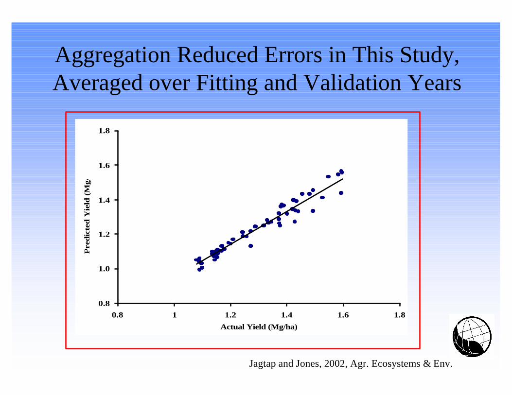
Aggregation Reduced Errors in This Study, Averaged over Fitting and Validation Years

Conclusions

• Yield bias must be removed when using crop models to predict regional yields

• RMSE averaged 14% when predicting yields for independent years, after correcting for bias

• Bias varied considerably across the state of Georgia, implying variations in management and other factors not accounted for in the model

• Other approaches may further reduce bias (see Irmak et al.)


Yield Forecast Tool

• Conditioned on:– Climatology

– Climate Forecast

Time

TodayStart of Season

Future – Use climatology or forecastHistory – Use recorded weather

Predicted yield in 1994 for Cerro Gordo Co., IA

using 7 forecast dates

1000

1500

2000

2500

3000

3500

4000

160 180 200 220 240 260 280 300Yield Forecast Date

Yield,

kg/

Maximum Yield

Mean Yield

Minimum Yield

Measured Yield

Maturity Date Range

1994

From W. D. Batchelro et al.

F a m i n e E a r l y W a r n i n g i n B u r k i n a F a s o - - A C a s e S t u d y o f M i l l e t

P r o d u c t i o n• S c o p e f o r i m p r o v e m e n t i n y i e l d f o r e c a s t i n g m e t h o d s f o r mil le t a n d s o r g h u m i n t h e S a h e l

• P o t e n t i a l l y h i g h v a l u e o f i n f o r m a t i o n b e c a u s e o f t h e p o l i c y i m p l i c a t i o n s ( a l l e v i a t i o n m e a s u r e s )

• A p r o o f - o f- c o n c e p t c a s e s t u d y , i n v o l v i n g t h e a s s e m b l y of soi l s , sa te l l i t e ra in fa l l data , c rop m o d e l s , g o v e r n m e n t s t a t i s t i c s

T h o r n t o n e t a l . , 1 9 9 7 . A g r . & F o r . M e t e o r o l o g y 8 3 : 9 5 - 1 1 2 .

S A T E L L I T E - D E R I V E DC R O P U S E I N T E N S I T Y

Provincial AreaPlanted to Millet

P R O V I N C I A L S T A T I S T I C SProduction and Yield

Averages

M I L L E T

M O D E L

S O I L S

Profi le Data

W E A T H E RLong -term

Histor ical Data

P R O V I N C I A L Y I E L D SUnique Combinat ions of

Soi l and Weather

A N O M A L Y T I M E S E R I E S

Dekad

%

16 17 18 19 ...

100

M E T E O S A T I M A G EDekadal RainfallEst imate (RFE)

G E O G R A P H I C I N F O R M A T I O N

S Y S T E M

P R O V I N C I A L P R O D U C T I O N

Season Product ion AnomalyDekadal Estimate of Current


How it was Done

R a i n f a l l E s t i m a t e : D e k a d 2 5 , 1 9 9 0

0

1 - 1 0

1 1 - 2 0

2 1 - 3 0

3 1 - 4 0

4 1 - 5 0

5 1 - 6 0

> 6 0

M i l l i m e t r e s

Met. station


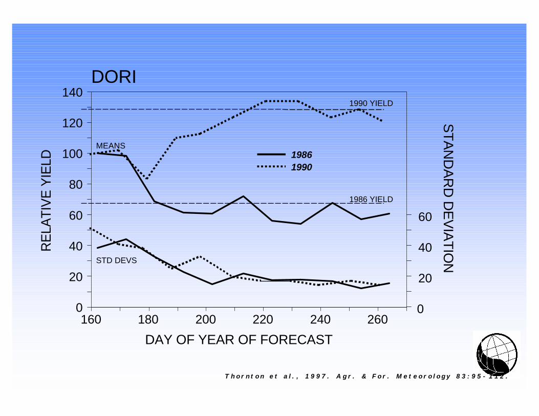
160 180 200 220 240 260

140

120

100

80

60

40

20

0

RE

LATI

VE

YIE

LD

DAY OF YEAR OF FORECAST

ST

AN

DA

RD

DE

VIA

TIO

N

60

40

20

0

1986 YIELD

1990 YIELD

MEANS

STD DEVS

DORI

19861990


S i m u l a t e d M i l l e t Y i e l d A n o m a l i e s , 1 9 8 6


Conclusions

• Satellite-derived rainfall, coupled with generated temperature and solar radiation values, have potential for early warning yield forecasts

• Yields forecast at mid season were within 15% of final yields

• Although more work is needed, this approach shows considerable promise


Regional Scale Crop Yield Predictions:

Discussion

predicting regional crop production: applicationsjhansen/jones16july.pdfgeorgia soybean yield...

Documents