predicting regional climate change: living with uncertaintytimm/papers/pipg-99.pdf · predicting...

Predicting regional climate change:living with uncertaintyTimothy D. Mitchell and Mike HulmeClimatic Research Unit, School of Environmental Sciences, University of East Anglia,Norwich NR4 7TJ, UK

A b s t r a c t : Regional climate prediction is not an insoluble problem, but it is a pro b l e mcharacterized by inherent uncertainty. There are two sources of this uncertainty: the unpre-dictability of the climatic and global systems. The climate system is rendered unpredictable bydeterministic chaos; the global system renders climate prediction uncertain through the unpre-dictability of the external forcings imposed on the climate system. It is commonly inferred fromthe differences between climate models on regional scales that the models are deficient, butclimate system unpredictability is such that this inference is premature; the differences are dueto an unresolved combination of climate system unpredictability and model deficiencies. Sincemodel deficiencies are discussed frequently and the two sources of inherent uncertainty arediscussed only rarely, this review considers the implications of climatic and global systemunpredictability for regional climate prediction. Consequently we regard regional climateprediction as a cascade of uncertainty, rather than as a single result process sullied by modeldeficiencies. We suggest three complementary methodological approaches: (1) the use ofmultiple forcing scenarios to cope with global system unpredictability; (2) the use of ensemblesto cope with climate system unpredictability; and (3) the consideration of the entire response ofthe climate system to cope with the nature of climate change. We understand regional climatechange in terms of changes in the general circulations of the atmosphere and oceans; so weillustrate the role of uncertainty in the task of regional climate prediction with the behaviour ofthe North Atlantic thermohaline circulation. In conclusion we discuss the implications of theuncertainties in regional climate prediction for research into the impacts of climate change, andwe recognize the role of feedbacks in complicating the relatively simple cascade of uncertaintiespresented here.

Key words: climate change, climate modelling, downscaling, external forcing, regional climateprediction, uncertainty, unpredictability.

I Introduction

When a person, city or nation considers climate change, their primary interest is inchanges in the warmth, rain and wind that affect them and their local environments.

Progress in Physical Geography 23,1 (1999) pp. 57–78

© Arnold 1999 0309–1333(99)PP214RA

58 Predicting regional climate change: living with uncertainty

Nevertheless, it was the argument that greenhouse gases emitted by humans (‘anthro-pogenic emissions’) might substantially alter global climate that persuaded the globalcommunity to establish the UN Framework Convention on Climate Change(UN/FCCC) (Hecht and Tirpak, 1995) with the following objective: ‘Stabilisation ofgreenhouse gas concentrations at a level that would prevent dangerous anthropogenicinterference with the climate system’ (UN/FCCC Article 2). The scientific evidence thatprompted countries to sign and ratify the UN/FCCC and then to negotiate the KyotoProtocol in 1997 (which sets specific targets for reducing greenhouse gas emissions –Masood, 1997) has been summarized in a series of influential reports prepared by theIntergovernmental Panel on Climate Change (IPCC) (Houghton et al., 1990; 1996). Themajority of the scientific evidence contained in these reports is concerned with the globalresponse of the climate system to anthropogenic forcing, but people, cities and nationswill be affected by the regional1 responses. The IPCC (Watson et al., 1998) was thereforeasked to prepare a special report on the vulnerability of natural environments andhuman societies to climate change in different regions of the world, which was toprovide: ‘A common base of information regarding the potential costs and benefits ofclimatic change, including the evaluation of uncertainties, to help the COP [Conferenceof the Parties to the UN/FCCC] determine what adaptation and mitigation2 measuresmight be justified’ (Obasi and Dowdeswell, 1998: vii).

Such accurate and precise information is highly desirable, but the chair of the IPCCwas forced to acknowledge that it could not be provided: ‘Because of the uncertaintiesassociated with regional projections of climate change, the report necessarily takes theapproach of assessing sensitivities and vulnerabilities of each region, rather thanattempting to provide quantitative predictions of the impacts of climate change’ (Bolinet al., 1998: x). Underlying this acknowledgement is the belief that ‘models cannotpredict on regional scales’. Examples of this frequently heard refrain may be taken froma single volume of Progress in Physical Geography (Joubert and Hewitson, 1997: 52;Schulze, 1997: 118; Wilby and Wigley, 1997: 531) or from Henderson-Sellers’ (1996: 59)review of the climate research process: ‘Unfortunately, numerical climate models andthe associated tools currently used to predict climate change, have no regionalprediction skill.’ If we regard GCMs (‘general circulation models’ or ‘global climatemodels’) as unreliable at regional scales, and if we regard the palaeo-analogue approachto regional climate prediction as inappropriate (Covey, 1995; Crowley, 1997), then itappears that regional climate prediction is not yet possible.

In this review we demonstrate that if we equip ourselves with an understanding ofthe fundamental role of uncertainty, then the prediction of regional climate change isreduced from an insoluble to a difficult problem. Since it is commonly assumed thatmodel deficiencies are responsible for any differences between models at regionalscales, such differences are commonly used as ‘proof’ that ‘models cannot predict onregional scales’. Having outlined in section II the differences between models atregional scales, we discuss in section III the potential for downscaling techniques toovercome the difficulty posed by the differences; we conclude that downscalingtechniques cannot correct for model inaccuracies and so they fail to overcome thed i ff i c u l t y. In section IV we consider the possibility that model deficiencies areresponsible for the differences between models at regional scales. However, there is analternative explanation provided by climate system unpredictability, and in section Vwe show that the dependence on initial conditions of a climate simulation means that

it is premature to infer from the differences between models at regional scales that themodels are deficient. Differences between simulations may (at least partly) be due to theinherent unpredictability of the climate system.

Therefore, if we consider the problem of predicting regional climate change in moregeneral terms we find that in addition to the possibility that model deficiencies mayrender our predictions uncertain (section IV), there are two sources of inherentuncertainty in regional climate prediction: climate system unpredictability (section V)and global system unpredictability (section VI). By ‘global system unpredictability’ ismeant the inherent unpredictability of the external3 forcings imposed on the climatesystem, whether anthropogenic (e.g., greenhouse gas emissions) or natural (e.g., solarvariability or volcanic eruptions). The unpredictability of the climatic and globalsystems is such that even with a perfect model, uncertainty would remain inherent toregional climate prediction. Yet the climatic and impacts research conducted thus farhas largely considered uncertainty in terms of model deficiencies. Therefore wesuggest (in section VII) that the problem of regional climate prediction should beviewed in terms of a cascade of uncertainty that stems from the unpredictability ofthe climatic and global systems, instead of a single result process sullied by modeldeficiencies.

Given this understanding of the uncertainties involved in regional climate prediction,in section VIII we suggest three methodological approaches to deal with them: (1) theuse of multiple forcing scenarios to cope with global system unpredictability; (2) theuse of ensembles to cope with climate system unpredictability; and (3) the considera-tion of the entire response of the climate system to cope with the nature of climatechange. All three approaches apply equally to global and regional climate prediction,but the entire response of the system to forcing (the third approach) is treateddifferently at global and regional scales. So in section IX we show how regional climateprediction is concerned in particular with the response of the general circulations ofthe atmosphere and oceans. In section X we illustrate this discussion by consideringthe North Atlantic thermohaline circulation, and by providing some examples of theuse of ensembles. In conclusion (section XI), we consider the implications of theuncertainty of regional climate prediction for research into the impacts of climatechange, and we point out the role of feedbacks in complicating the relatively simplecascade of uncertainties presented here.

II Intermodel differences on regional scales

In the early 1990s there was very little confidence in the regional climate informationextracted from GCM integrations, and the models were held responsible because of

• the equilibrium method of forcing models with CO2-equivalent gases;• the lack of fully coupled atmosphere–ocean GCMs (AOGCMs);• coarse model resolution;• deficiencies in the model physics;• an inability to simulate present-day regional climate features; and• intermodel differences in simulations of regional climate change.

Timothy D. Mitchell and Mike Hulme 59


Since then there have been a number of improvements in the climate models, notablyin the adoption of transient methods of forcing with CO2-equivalent gases, and in thedevelopment of fully coupled AOGCMs.

Despite the improvements in the climate models, intermodel comparisons still revealsubstantial intermodel differences on regional scales. The IPCC Second assessment reportincluded a comparison of simulations from a number of AOGCMs for five particularregions (Kattenberg et al., 1996), and more recent work (Kittel et al., 1998) has confirmedthe results reported by the IPCC. The models’ representation of the real world may bejudged by comparing the control simulations4 with observed climatologies; suchcomparisons reveal that the biases in the seasonal cycle range between –7 °K and 10 °K.These recent model experiments exhibit biases in the same range as those in the IPCCFirst assessment report for control simulations with older models (Gates et al., 1990). If wecompare the models we find that over most regions the intermodel range oftemperature bias is of the order of 10 °K, and when AOGCMs are forced withgreenhouse gases, the climate ‘scenarios’5 of regional temperature and precipitationchange vary widely from model to model (Kattenberg et al., 1996; Kittel et al., 1998).Figure 1 illustrates this variety of regional responses to forcing that a collection ofmodels typically exhibits. Even when one considers a global-scale phenomenon such asENSO (El Niño Southern Oscillation), both the model differences from observations,and the wide range of results among models and between models and observations,

Figure 1 The differences between models on regional scales. Ninemodel experiments (represented by different symbols) were reviewedby Kattenberg et al. (1996) who presented the regional biases insummer (JJA) temperature and precipitation for seven regions (theeighth (GL) is a global average). Temperature biases are differences(control minus observed); precipitation biases are differences aspercentages of the observed. Square brackets about the zero-bias linespan +σ to –σ for temperature, or the coefficient of variation forprecipitation, of observed regional averagesSource: Modified after Kittel et al. (1998)

remain; a model’s ENSO may be too strong (Tett et al., 1997), too weak (Knutson andManabe, 1994; Schneider and Kinter, 1994), or absent (von Storch, 1994). Intermodelcomparisons such as these have reduced our confidence in AOGCM scenarios ofregional climate change to a ‘low’ level (Kattenberg et al., 1996: 339), and the culprit isgenerally held to be the AOGCMs’ low horizontal resolution and physical parameteri-zations (Gates et al., 1996).

III Can downscaling help?

Intermodel differences have discouraged many researchers from using AOGCM outputon regional scales. Being aware of the acute need for reliable predictions of regionalclimate change, some have therefore turned to downscaling techniques in theirattempts to overcome the differences between models on regional scales. Recentreviews of downscaling techniques may be found in Hewitson and Crane (1996),Kattenberg et al. (1996) and Wilby and Wigley (1997). Statistical downscaling techniquescommonly develop statistical relationships between local climate variables and modelpredictors, and then apply those relationships to model climate scenarios to deriveestimations of localized climate change. Such statistical links may be made directly byregression (Kim et al., 1984), via circulation patterns (Wilby, 1994) or via stochasticweather generators (Wilks, 1992). Dynamical downscaling techniques commonly useoutput from GCM simulations to provide the boundary and initial conditions for a‘one-way nested’ regional model with a higher spatial resolution (Giorgi, 1990); avariant approach is to develop a variable-resolution GCM (Deque and Piedelievre,1995; Fox-Rabinovitz et al., 1997).

When applied to regional climate change prediction, the one element thesedownscaling techniques have in common is their dependence upon the accuracy of thelarge-scale information with which they are ‘driven’. This is true whether the relation-ship between the predictor and predictand is statistical or dynamical; both assume thatthe large-scale information from the GCM is ‘correct’ and on that basis they attempt toestimate the corresponding local change in climate. If the large-scale changes in theGCMs are inaccurate, then the derived local changes merely add misleading precisionto the GCM results, and the downscaling techniques fail to add any predictive skill.Figure 2 illustrates how closely a downscaled variable depends on the GCM variablefrom which it is derived. We find that if the GCM variable is an accurate representationof the corresponding observed variable then the downscaled variable is also an accuraterepresentation of the observed variable; conversely, where the GCM variable isinaccurate, so is the downscaled variable. We conclude that a pre requisite ofdownscaling is an accurate GCM to ‘drive’ the downscaling technique. LeonardBengtsson (1995), former Director of the Max Planck Institute and ECMWF, concurs:‘Regional climate prediction requires first and for all [sic] good global prediction bycoupled climate models – without it regional simulations are useless.’ The developmentof downscaling techniques does not overcome the lack of confidence in AOGCMs atregional scales; it merely accentuates the need for the inherent regional uncertaintiesto be understood.



IV AOGCM deficiencies

Any attempt to explain the wide range of AOGCM outcomes at regional scalesdescribed in section II must consider a number of competing potential reasons, the firstof which is provided by model deficiencies. Most scientists accept that it is unreason-able to suggest that AOGCMs simply have poor physics and are unrepresentative ofreality. If one allows for the coarse resolution of AOGCMs then the models areremarkably good, simulating the seasonal cycles in temperature, precipitation rates andmean sea-level pressure (Gates et al., 1996).

However, it is possible that the parameterizations, coarse resolution and unrepre-sented feedbacks that limit AOGCMs may generate the intermodel variety exhibited inAOGCM simulations at regional scales. This may particularly apply to hydrologicalvariables, whose key processes (evaporation, convection, condensation and precipita-tion) are all highly discontinuous in space and time and are heavily parameterized inAOGCMs. Such model inaccuracies are a commonly recognized source of uncertaintyin climate prediction. However, in practice it is difficult to judge the effect of suchmodel weaknesses in isolation from another source of uncertainty that provides afurther potential reason for the wide range of model outcomes at regional scales:climate system unpredictability.

Figure 2 The dependence of downscaled results on the large-scaleinformation supplied by the GCM for three variables: maximum dailytemperature in degrees Celsius (TMX), fog in units 0–1 (FOG) andsnow height in cm (SNW). The observed data (OBS), the GCM data(CTL) and the downscaled data (SCA) are presented for the weatherstation at Potsdam, GermanySource: Modified after Bürger (1996)

V Climate system unpredictability

We may generalize the problem of regional climate prediction to all natural systems andstate that if the natural system bears the characteristics of a chaotic system6 then if (in ahypothetical situation) it evolved a number of times from slightly different initialconditions, it would exhibit different characteristics in each evolution. The differentoutcomes might be described in terms of a frequency distribution of possible outcomes.If we model such a natural system then we expect (and hope) that successiveevolutions, with slightly different initial conditions, will also exhibit different charac-teristics. Our evaluation of the worth of the model will not be on the grounds ofwhether or not the model possesses a frequency distribution of possible outcomes, butof whether or not the model’s distribution corresponds to the distribution of the naturalsystem.

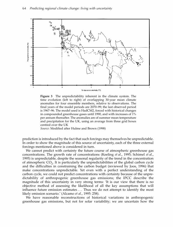
Since the climate system is commonly regarded as a chaotic system (Lorenz, 1963;1993) we expect that multiple integrations of an AOGCM, with slightly different initialconditions, will yield a frequency distribution of possible outcomes. Figure 3 displaysfour separate evolutions of a single model where only the initial conditions variedbetween evolutions; the wide divergence between the outcomes illustrates the unpre-dictability inherent to the climate system. So we are not surprised at the occurrence ofintermodel differences at regional scales; we would expect differences to occur even ifthe AOGCMs were identical.

It follows that in the presence of such unpredictability, the argument that ‘there is awide range of model outcomes, therefore the simulations are inaccurate’ (often with thethought that this is due to parameterizations or coarse resolutions) is a non sequitur. Anunexplored possibility in such an argument is that the unpredictability of the climatesystem may support a frequency distribution of possible outcomes, and that the widerange of model outcomes may be due to accurate modelling of this distribution, ratherthan to inaccurate AOGCMs diverging from a single solution. Therefore it is prematureto state that ‘models cannot predict on regional scales’ merely from the evidencereviewed in section II. Rather, we must ask whether the model distribution of outcomesis a good representation of the distribution of outcomes possessed (theoretically) by thenatural system or whether it has been corrupted by poor parameterization schemes, bycoarse AOGCM spatial resolution or by unrepresented external phenomena (such asvegetation feedbacks or solar variability). The extent to which the wide range of modeloutcomes is due to the unpredictability inherent to the climate system over againstAOGCM deficiencies is still an open question.

VI Global system unpredictability

A second source of inherent uncertainty in regional climate prediction is ‘global systemunpredictability’, which encompasses all the unpredictabilities bound up in the futureexternal forcings imposed on the climate system. These external forcings may bea n t h ropogenic or natural; some of the most important include anthro p o g e n i cgreenhouse gas emissions, solar variability and volcanic eruptions. Any accurateclimate prediction must take into account the effect of such external forcings on theclimate system, and our second source of inherent uncertainty in regional climate



prediction is introduced by the fact that such forcings may themselves be unpredictable.In order to show the magnitude of this source of uncertainty, each of the three externalforcings mentioned above is considered in turn.

We cannot predict with certainty the future course of atmospheric greenhouse gasconcentrations. The growth rate of concentrations (Keeling et al., 1995; Schimel et al.,1995) is unpredictable, despite the seasonal regularity of the trend in the concentrationof atmospheric CO2. It is particularly the unpredictabilities of the global carbon cycleand the difficulties in constraining the carbon budget (reviewed by Joos, 1996) thatmake concentrations unpredictable. Yet even with a perfect understanding of thecarbon cycle, we could not predict concentrations with certainty because of the unpre-dictability of anthropogenic greenhouse gas emissions; the IPCC describe themagnitude of this uncertainty in very strong terms: ‘It is our view that there is noobjective method of assessing the likelihood of all the key assumptions that willinfluence future emission estimates . . . Thus we do not attempt to identify the mostlikely emission scenario.’ (Alcamo et al., 1995: 258).

We have reasonable reconstructions of historical variations in anthropogenicgreenhouse gas emissions, but not for solar variability; we are uncertain how the

Figure 3 The unpredictability inherent in the climate system. Thetime evolution (left to right) of overlapping 30-year mean climateanomalies for four ensemble members, relative to observations. Thefinal years of the model periods are 2070–99; the last observed periodis 1967–96. The model used is HadCM2, forced with historical changesin compounded greenhouse gases until 1990, and with increases of 1%per annum thereafter. The anomalies are of summer mean temperatureand precipitation for the UK, using an average from three grid boxescentred over the UKSource: Modified after Hulme and Brown (1998)

magnitude of solar forcing has varied in the past. The minimum magnitude of changewe can conceive is the irradiance change (0.15%) in the 11-year Schwabe cycle that hasbeen directly observed from satellites (Willson and Hudson, 1991) over the past twodecades. The maximum conceivable magnitude was estimated by Reid (1997) to be0.65%, by assuming that all the estimated global temperature variability since theMaunder Minimum of the seventeenth century may be attributed solely to solarvariability and to anthropogenic greenhouse gas emissions. More conservative recon-structions of solar variability have been published by Hoyt and Schatten (1993) and byLean et al. (1995), who calculate the difference in irradiance between the MaunderMinimum and the present to be 0.30% and 0.24%, respectively. If the historicalvariations in solar forcing are so uncertain – Reid describes the reconstructions asinstances of ‘a highly speculative activity’ (1997: 392) – then it is difficult to evaluate theeffects of solar variability on the climate system; indeed, Hoyt and Schatten admit onthe cover of their work entitled The role of the sun in climate change (1997) that they cannotanswer the question posed by the title. However, a succession of model experiments(Rind and Overpeck, 1993; Crowley and Kim, 1996) has suggested that solar variabilityis sufficient to force global climate changes of several tenths of a degree over centennialtimescales. This succession has culminated in AOGCM experiments (Cubasch et al.,1997; Tett et al., 1998) that confirm the potential importance of solar variability, butsuggest that solar forcing changes are insufficient by themselves to explain thetemperature record of the twenthieth century. Since the historical record of solarvariability is so uncertain, and since the historical effects of solar variability on theearth’s radiation budget are unknown, the solar forcing of climate in the future must beregarded as unpredictable.

Although the climatic effects of certain volcanic eruptions are well known, theclimatic forcing from volcanoes is unpredictable. Observations of the eruption plume ofMount Pinatubo in the Philippines (15 June 1991) demonstrated the atmospheric effectsof a major eruption in a remarkable way (McCormick et al., 1995); the albedo changes tothe atmosphere resulted in a peak decrease in August 1991 of 8 Wm–2 in radiativeforcing between 5 °S and 5°N, and of 3 Wm–2 globally (Minnis et al., 1993). Despite theglobal cooling, this eruption – like others – produced a pronounced warming in theNorthern Hemisphere (Robock and Mao, 1992; Parker et al., 1996) that illustrates thecontrast in climatic effects that may appear between global and subglobal scales.Although Mount Pinatubo was well observed, it is difficult to reconstruct the history ofvolcanic eruptions; even recent volcanoes may escape observation (e.g., Sedlacek et al.,1981; Mroz et al., 1983) and we are reliant upon proxy measurements for identifying thedates of major eruptions prior to the commencement of satellite observations (e.g.,Briffa et al., 1998). It is even more difficult to reconstruct the radiative forcing exertedupon the atmosphere by an eruption. The radiative forcing depends upon the nature ofthe injection of aerosols and aerosol precursors into the stratosphere, and upon thespatial and temporal patterns of their residence in the atmosphere. The location,altitude and period of injection all contribute to the former, and the particulate micro-physics, particulate chemistry and atmospheric circulation all contribute to the latter.Whereas there is a comparatively wide range of sources of information for identifyingthe dates of eruptions, the scope for identifying the characteristics of the plumes fromindividual eruptions is severely limited by the requirement for a wide range of evidence(e.g., de Silva and Zielinski, 1998). Bradley and Jones (1992: 618) conclude their



evaluation of volcanic forcing reconstructions as follows: ‘The record of large explosiveeruptions since AD 1500 is probably quite incomplete, making it difficult to assess theiroverall impact on climate.’ Predicting the characteristics of future volcanic eruptions iseven more difficult than reconstructing those of the past, and therefore the volcanicforcing of climate in the future is inherently unpredictable.

VII The cascade of uncertainty

The uncertainty concerning future regional climate change that results from climatemodel inaccuracies is commonly recognized. Yet the two sources of uncertainty that areinherent to regional climate prediction – the unpredictability of the climatic and globalsystems – have not been adequately dealt with in regional climate scenarios thus far,either in scenario construction, or in considering the environmental effects of thescenarios. Much of the research concerning the environmental effects of future climaticchange may be categorized into the ‘timeless’ and the ‘single scenario’ approaches. Theresearch summarized by the IPCC First assessment report (Houghton et al., 1990), andmuch of that summarized by the IPCC Second assessment report (Watson et al., 1996),considered the environmental impacts of a single physical event – such as the doublingof atmospheric concentrations of CO2 – in a ‘timeless’ approach that made no attemptto attach any time to the physical event. The introduction of transient perturbed climatechange experiments has permitted a time dimension to be introduced to impact studies,which is incorporated into some of the Second assessment report and the majority of theIPCC Regional report (Watson et al., 1998). However, such impact studies are commonlylimited to a ‘single scenario’, considering the environmental impacts at a number ofpoints in time of only a single climate realization produced by forcing only a singleAOGCM with only a single emissions scenario.

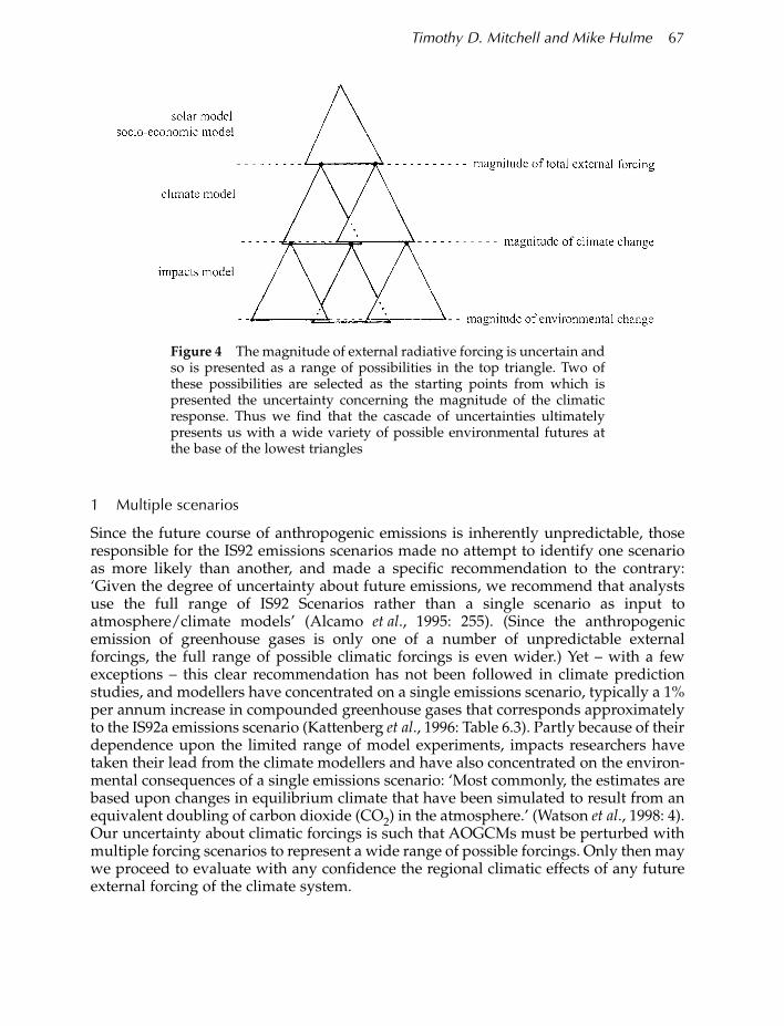
Thus our understanding of the regional consequences of climate change is marked bythe omission of any consideration of the uncertainties introduced by the unpredictabil-ity of the climatic and global systems. This neglect has permitted a ‘single result’approach to prediction to permeate the climate change impacts literature, an approachthat is condemned by Henderson-Sellers (1996: 60): ‘Since prediction is not a singleresult process, all predictions are (un)certain, contain and/or are based on, incompleteinformation and are debatable.’ The unpredictability of the climatic and global systemsintroduces a cascade of uncertainty to regional climate prediction (Figure 4) that cannotbe squeezed to the single point of the ‘single result’ approach to prediction.

VIII Three methodological responses

Since unpredictability is a system characteristic, even with a perfect model the problemof regional climate prediction would still be characterized by uncertainty. To live withthis uncertainty demands that we make three specific methodological responses: (1)the use of multiple forcing scenarios to cope with global system unpredictability; (2)the use of ensembles to cope with climate system unpredictability; and (3) the consid-eration of the entire response of the system to cope with the nature of climate change.We will comment briefly on each of these in turn.

1 Multiple scenarios

Since the future course of anthropogenic emissions is inherently unpredictable, thoseresponsible for the IS92 emissions scenarios made no attempt to identify one scenarioas more likely than another, and made a specific recommendation to the contrary:‘Given the degree of uncertainty about future emissions, we recommend that analystsuse the full range of IS92 Scenarios rather than a single scenario as input toatmosphere/climate models’ (Alcamo et al., 1995: 255). (Since the anthropogenicemission of greenhouse gases is only one of a number of unpredictable externalforcings, the full range of possible climatic forcings is even wider.) Yet – with a fewexceptions – this clear recommendation has not been followed in climate predictionstudies, and modellers have concentrated on a single emissions scenario, typically a 1%per annum increase in compounded greenhouse gases that corresponds approximatelyto the IS92a emissions scenario (Kattenberg et al., 1996: Table 6.3). Partly because of theirdependence upon the limited range of model experiments, impacts researchers havetaken their lead from the climate modellers and have also concentrated on the environ-mental consequences of a single emissions scenario: ‘Most commonly, the estimates arebased upon changes in equilibrium climate that have been simulated to result from anequivalent doubling of carbon dioxide (CO2) in the atmosphere.’ (Watson et al., 1998: 4).Our uncertainty about climatic forcings is such that AOGCMs must be perturbed withmultiple forcing scenarios to represent a wide range of possible forcings. Only then maywe proceed to evaluate with any confidence the regional climatic effects of any futureexternal forcing of the climate system.


Figure 4 The magnitude of external radiative forcing is uncertain andso is presented as a range of possibilities in the top triangle. Two ofthese possibilities are selected as the starting points from which ispresented the uncertainty concerning the magnitude of the climaticresponse. Thus we find that the cascade of uncertainties ultimatelypresents us with a wide variety of possible environmental futures atthe base of the lowest triangles


2 Ensembles

The inherent unpredictability of the climate system is such that our understanding ofwhat it means to ‘predict’ climate is somewhat different from the popular perception ofprediction.7 Even if we were able to force a perfect model with a perfectly specifiedexternal forcing scenario, the model would not follow a single trajectory through timethat might be calculated beforehand, in the manner of a frictionless pendulum. Rather,the dependence of the climate system on initial conditions means that inaccuracies inthe initial state grow through time, so that there is a multiplicity of future states that arepossible, even under a perfect forcing specification (Lorenz, 1963). This characteristicimposes limits of a few days on numerical weather prediction (James, 1994: 292–93), asour ability to forecast weather is dependent, not merely upon observational accuracy,computational power and the accuracy of the model, but more fundamentally upon the‘chaotic’ nature of the system. For this reason an operational meteorologist willconstruct an ‘ensemble’ of simulations when making a forecast. The single GCM isintegrated a number of times, the only difference between each ensemble ‘member’being the initialization conditions. The aim of constructing the ensemble is to samplethe full probability distribution of the future course of the weather. Likewise, if we aremaking predictions about future climate then we must accept that the climate system isunpredictable and that ensemble techniques should be used to sample the ‘full’probability distribution of the future course of climate. An examination of Figure 3illustrates the importance of the ensemble approach. If only one simulation had beenperformed with HadCM2 rather than four, then only a single climate scenario wouldhave been available and a misleading impression would have been gained of theregional climatic response to the perturbation.

3 Entire response of the system

We have addressed the two sources of uncertainty that are inherent to regional climateprediction, but we have not yet considered the nature of the regional climate changesthat we expect to find. Such climate changes are conceptually different from dailychanges in weather and so require a different kind of prediction. A change in theweather from Wednesday to Thursday may be understood in terms of a trajectory (theweather) in a fixed attractor8 (the coupled atmosphere–ocean system). A weatherforecast is an instance of what Lorenz (1975) described as predictions ‘of the first kind’.It is an initial value problem, where we are given a set of initial conditions fromWednesday and we must calculate from them the future behaviour of the atmospherein order to derive Thursday’s conditions. In contrast, we may understand a change inradiative forcing (perhaps from increased greenhouse gas concentrations or fromchanges in solar irradiance) as effecting a change in the attractor. We do not expect theattractor of the climate system to change in response to forcing in a linear manner, suchas in a linear shift of the time-averaged state against an unchanged variabilitybackground (Figure 5); rather, we expect the system response to perturbation to dependupon the convolution of the forcing with the ‘natural’ variability of the system (Figure6). A climate prediction is an attempt to predict how the attractor will change (aprediction ‘of the second kind’9 – Lorenz, 1975); in this sense any climate predictionmust consider the entire response of the system.

IX Characterizing the entire response of the system

Climate system predictions of the second kind may be examined from global orregional perspectives. These perspectives characterize the entire response of the systemin different ways. It is worth considering this contrast between the global and theregional, not merely to avoid confusion, but to illustrate what is meant by consideringthe ‘entire response of the system’.

In global climate analyses we often consider a single change characterized – in ahighly simplified manner – as a linear shift. We treat the variability as ‘noise’, we treatthe shift as ‘signal’ and we use noise reduction techniques to increase the signal-to-noise ratio so that we may claim ‘detection’ of a statistically significant shift (Santer et


Figure 5 An erroneous linear-thinking perspective might supposethat a forcing (F) imposed on the Lorenz model (a) would produce animpact similar to (b)Source: Palmer (1993)


al., 1996). One particular group of ‘detection studies’ adopting this approach (Santer etal., 1994; Hegerl et al., 1996; 1997) perturbed an AOGCM with increased atmosphericgreenhouse gas concentrations, employed noise reduction methods to extract a patternof response from the model output, and compared the pattern with patterns derivedfrom observations. Such ‘fingerprint studies’ culminated in the tentative claim(Houghton et al., 1996) that anthropogenically induced climate change had beendetected. The motive behind these detection studies was to encourage the adoption ofmitigation policies by quantifying and confirming the conclusion that may be drawnfrom a simple consideration of the radiative properties of the global climate system(Arrhenius, 1896a; 1896b).

Since the detection studies described above consider a single global response toexternal forcing, it is only at the continental, hemispheric and global scales that theymay be expected to achieve the identification of a response (Stott and Tett, 1998).However, the information required for adaptive responses to climate change must be onregional scales. If we consider the response to radiative forcing of a particular regionthen we can no longer treat changes in the general circulations of the atmosphere andoceans as ‘noise’ to be disregarded in favour of a single linear shift, because thatregion’s climate is a result of those general circulations. It is through the general circu-lations that energy is redistributed in such a way as to maintain in equilibrium thezones of permanent radiation surplus and deficit, and any radiative forcing of theclimate system ‘reaches’ a particular region through these dissipative mechanisms. So

Figure 6 If a forcing (F) is imposed on the Lorenz model along thepositive T-axis, then the (counterintuitive) impact is a decrease in T.This can be understood by noting that near the region of maximuminstability, positive T forcing increases the probability that the systemwill evolve towards the regime whose centroid has the smaller valueof TSource: Palmer (1993)

we are required to understand the behaviour of, and the effects of radiative forcingupon, the general circulations if we are to understand the consequent climatic changesin a particular region. In short, we need to understand the ‘entire response of thesystem’ in more detail than at the global scale.

This explanation of regional climate change in terms of changes in the general circu-lations of the atmosphere and oceans is a ‘geographical’ equivalent to the ‘mathemati-cal’ explanation, given above, in terms of a change in the climate system attractor. Thegeneral circulation changes correspond to the changes in the attractor. The general cir-culations and the attractor incorporate a natural variability that extends from secondsto millennia, and the trajectory through the attractor is inherently unpredictable. Theregional climate change problem is – assuming that the radiative forcing is perfectlyspecified – to elucidate how the general circulations will change or, expressed alterna-tively, to elucidate how the shape of the climate system attractor will change. It is in thissense that we need to understand the ‘entire response of the system’. However, on theinterdecadal timescales of interest for climate prediction we hardly understand thecurrent behaviour of the general circulations – Latif (1998) provides a good review – letalone the effects of external forcing upon them. The position is summed up well byAnderson and Willebrand (1996: v) in their work on decadal climate variability: ‘Thecauses of natural variability of the climate system on decadal time scales are presentlynot well known; understanding the mechanisms is however a prerequisite for anyclimate prediction of changes on these time scales.’

X Some examples

The discussion in this review has necessarily been of a rather theoretical nature, and itis appropriate to introduce some examples.

A brief consideration of the thermohaline circulation (THC) of the North Atlanticserves to illustrate a number of points. In 1961 Stommel reported a very simpleexperiment with profound results that was forgotten until the 1980s. He considered theconvective behaviour between two interconnected reservoirs forced by densitydifferences maintained by salt and heat transfers and found that two distinct stableregimes were possible. Building on this work, Welander (1986) later presented anassortment of thermohaline oscillators and multiple steady states applicable to theworld’s oceans. So multiple steady states are conceivable under natural variability.More recently, researchers have shown that anthropogenic external forcing may affectthe behaviour of the THC to the extent of inducing a switch between one climatic stateand another. Manabe and Stouffer (1993) chose two different emissions scenarios withwhich to force a coupled model, and examined the response in the North Atlantic THC;they found two distinct stable regimes, the occupancy of which depended on themagnitude of the equilibrium change in atmospheric CO2 concentration. In a similarexperiment, Stocker and Schmittner (1997) showed that the stable regime obtained isalso dependent upon the rate of change of atmospheric CO2 concentration. Rahmstorf(1995) conducted a more general examination of the hysteresis behaviour of the NorthAtlantic THC and found a number of forms of nonlinear behaviour. Schiller et al. (1997)considered the stability of the North Atlantic THC against meltwater input and foundthat four elements of the climate system exhibited feedbacks with the THC: oceanic heat



transport, precipitation and runoff, the atmospheric circulation and the wind-drivencirculation.

This nonlinear behaviour of the North Atlantic THC on decadal and centennialtimescales illustrates the unpredictability of the coupled ocean–atmosphere system thatwas discussed in section V. It suggests that climate predictions for regions dependentupon the North Atlantic THC (principally Europe) must be made on the understandingthat an external forcing may result in a number of possible outcomes (section VII). Sincethe behaviour of the North Atlantic THC depends on the magnitude and rate ofexternal forcing, any predictions should be made on the basis of AOGCM simulationsin which the model is forced with multiple forcing scenarios (section VIII 1). Since thebehaviour of the North Atlantic THC depends on the initial conditions, an ensembleexperiment should be performed for each forcing scenario (section VIII 2). Since anyexternal forcing affects the North Atlantic THC through the atmosphere and continentalice sheets, and since the THC itself influences the atmosphere and continental icesheets, the North Atlantic THC response to forcing can only be understood in terms ofthe entire response of the system to forcing (sections VIII 3 and IX).

Our second example concerns the application of ensemble methods that (as wesuggested in section VIII 2) allow us to deal with climate system unpredictability inregional climate prediction. There are not yet many instances of ensemble techniquesbeing used in the climate change problem, chiefly because of the expense of performingmulticentury AOGCM experiments. (Therefore it is also worth considering the use ofensemble techniques in the seasonal prediction problem – Dix and Hunt, 1995; Rowell,1998.) The Max-Planck Institute (Cubasch et al., 1997) have performed a two-memberensemble experiment that is relevant to the climate change problem, in which ECHAM3was forced with an estimated historical record of solar variability. The Hadley Centrehave performed a wider range of four-member ensemble experiments in whichHadCM2 was forced with estimated historical and future atmospheric CO2 andsulphate concentrations (Mitchell et al., 1999), and with estimated historical records ofsolar and volcanic variability (Tett et al., 1998). An example of the uses to which theHadley Centre ensembles have been put is provided by the analysis on the NorthernHemisphere storm tracks in general (Carnell and Senior, 1998), on the North AtlanticOscillation in particular (Osborn et al., 1999), and on water and crop responses toclimate change in Europe (Hulme et al., 1999).

XI Conclusion

This discussion of the uncertainty bound up with regional climate prediction has manyimplications for research, both of the climate system itself and of the impacts of climatechange. It has been shown that even with a perfect model, uncertainty would remaininherent to regional climate prediction, because of the inherent unpredictabilities ofexternal forcing – both anthropogenic and natural – and of the climate system itself.Only if we were able to alter the fundamental natures of the climate and global systemsto make them predictable might we hope to predict with certainty. It seems that if weare to be successful in our aim of predicting regional climate change then we mustunderstand that uncertainty must arise from systemic unpredictability.

The first implication of this insight is that to avoid misunderstanding we must adopt


the precise terminological language that contrasts unpredictability (a system character-istic) with uncertainty (what we have to live with as a consequence of unpredictability),and that treats ‘prediction’ in the context of inherent uncertainty. A further implicationis that we must not treat any model output as the one true climate prediction, but musttake the different – and equally probable – climate scenarios illustrated in Figure 3 anduse them as equally probable inputs when researching the impacts of climate change.

The uncertainties involved complicate the communication of vital information,making scientists instinctively wary of making any assessment of the changes that mayfollow anthropogenic forcing. So when pressed for information, scientists are facedwith a classic dilemma: predict and risk being wrong, or remain silent and risk failingto release useful information. Fowler and Hennessy (1995: 284) discuss the problem forthe specific issue of extreme precipitation events and are convinced of the need forscientists to be vocal:

Although there are good reasons for scientific reticence concerning possible changes . . . there is also a pressingneed for information . . . In the absence of contrary advice from atmospheric scientists, the norm will prevail ofassuming that past experience is a reliable guide. Given that the implicit assumption of a stationary climateunderlying such an approach contradicts expectations of a rapidly changing climate over the next severaldecades, clearly there is an onus on atmospheric scientists to provide as much information as possible.

The inherent uncertainty in regional climate prediction is such that scientists mustcounter the damaging norm of assuming a stationary climate. In the past, conventionalunderstanding has adopted a 30-year mean as the one true climate and this humanartifact has been used as the basis upon which return periods are calculated, infra-structure is designed and policy decisions are reached. Thus humans are only adaptedto the latest 30-year mean, rather than to true levels of natural variability. To be in aposition to adapt to the climatic changes that will follow any future anthropogenicforcing of the climate system, we must first be better adapted to the levels of variabilitypresent in an unperturbed climate system. Achieving this requires a better understand-ing both of climatic variability and of the sensitivity of natural environments andhuman societies to that climatic variability.

The problem for researchers is to close the gap between the demand for, and supplyof, reliable information on regional climate change and its impacts. At this point it ishelpful to make a distinction between the information necessary for mitigation ratherthan for adaptation by policy decisions. Since CO2 emissions are rapidly mixed in theatmosphere, the climate system response to CO2 emissions is spatially global in scale.So mitigation policy , which seeks to reduce CO2 emissions, requires information aboutthe global-scale response to CO2 emissions (the existence of a ‘shift’ in the climatesystem attractor); the ‘detection’ work described in section IX has sufficiently suppliedthat requirement for the global community to sign the UN/FCCC and the KyotoProtocol. In contrast, adaptive responses to climate change require information onregional scales. Yet regional climate prediction is still in its infancy, so a large gapremains between the demand for, and supply of, reliable information. There is also acontrast between the objects of the mitigative and adaptive responses. The adaptivestrategies require that a response be made to the climate system’s behaviour, whetherthe system is being forced by humans or by natural phenomena. Mitigative strategies,however, can only deal with the anthropogenic forcing of the climate system – unlesswe are so bold as to contemplate altering solar variability or volcanic eruptions.


This review has presented the cascade of uncertainties (Figure 4) as the reality withwhich our methodologies must live. None the less we recognize that there are twoproblems with limiting the regional climate prediction problem to the resolution of thisrelatively simple cascade of uncertainties. The first problem is the presence of feedbacksbetween most of the nonhuman elements of the cascade. This is well exemplified by theexchanges between the coupled atmosphere–ocean–cryosphere system (simulated byAOGCMs) and the land surface, such as the posited vegetation feedbacks in the Sahel(reviewed by Nicholson, 1988) that may be partly responsible for the prolongeddroughts of recent decades (Eltahir and Gong, 1996). Another example refers to thepotential, described in section X, for multiple steady states in the thermohalinecirculation. Rahmstorf (1995) has shown with a coupled model that it is conceivable thatp recipitation changes may change freshwater inputs into the oceans, triggeringconvective instability, and thus inducing transitions between different equilibriumstates of the thermohaline circulation, with substantial climatic effects.

The second problem is the lack of attention to humans. The human world is unpre-dictable; only the most extreme reductionist can envisage the predictability of humanthought and behaviour. Since humans affect the climate system and the consequencesin turn affect humans, we cannot completely account for all the interactions that are ofrelevance to regional climate prediction. Of course, we try to include all the possibilitiesof human influence on the climate system through the emissions scenarios, but thisneglects the feedbacks between humans and their environment.

Integrated assessment (Peck and Teisberg, 1992; Nordhaus, 1994; Hasselmann et al.,1997) is another venture still in its infancy, but in the long run it may make aninvaluable contribution to unravelling the web of feedbacks and to managing globalchange. Whatever the contribution made by integrated assessment, we must stillhowever carefully examine each environmental system for its response to regionalclimate change, with a keen awareness of the inherent uncertainties involved. If we areto adapt sensitively to climate change then we require information now; the manyuncertainties involved should not stop us from providing the best information possible.The heart of the task of regional climate prediction lies in bringing to light the differentpossibilities the future may hold for us; we must elucidate the climatic and environ-mental changes that are possible and enlighten nonscientists in ways that communicatethe inherent uncertainties of regional climate change.

Acknowledgements

Tim Mitchell is supported by a grant from the Natural Environment Research Council(GT 04/97/81/MAS) in conjunction with the UK Meteorological Office (Met 1b/2437),but the views expressed in this article are solely those of the authors, not of NERC orUKMO. We are grateful to Dr Declan Conway for his comments on a draft of this article,and to Dr John Mitchell for his support and constructive discussions.

Notes

1. In this review ‘regional’ refers to subcontinental and local scales.2. In current terminology ‘adaptation’ measures are adaptive responses to an actual climate


change, past, present or future; ‘mitigation’ measures are responses to a perceived potential futureclimate change that attempt to reduce the likelihood of that change occurring. An example of theformer is building more coastal defences; and an example of the latter is reducing greenhouse gasemissions.

3. In this review any agent or system beyond the scope of the atmosphere, oceans and cryosphereis considered to be ‘external’ to the climate system. Thus external forcings on the climate systeminclude both anthropogenic and natural forcings, exemplified by CO2 emissions and solar variability,respectively.

4. A control simulation is conducted without any ‘perturbation’ from humans, the sun or any otherexternal agent.

5. The term ‘scenario’ has been much abused (see Henderson-Sellers, 1996). In this review an‘emissions scenario’ refers to a description of a possible future temporal pattern of anthropogenicemissions of greenhouse gases; a ‘climate scenario’ refers to a description of a possible future climate.

6. An introduction to deterministic chaos is beyond the scope of this review, and the reader isreferred to Hall’s (1991) introduction to chaos and Lorenz’s (1993) introduction to chaos with itsparticular reference to the atmosphere.

7. Palmer (1993) provides a good introduction to these predictability concepts.8. The climate system ‘attractor’ may be loosely defined as the complete set of possible instanta-

neous states of the climate system, or more precisely as ‘a limit set that is not contained in any largerlimit set, and from which no orbits emanate’ (Lorenz, 1993: 206).

9. These two ‘kinds’ of prediction – discussed at greater length by Palmer (1996) – are fundamen-tally different, and it is crucial to understand this difference when interpreting GCM output, especiallysince the same GCM may be used for both kinds of prediction (Cullen, 1993).

References

Alcamo, J., Bouwman, A., Edmonds, J., Grubler ,A., Morita, T. and Sugandhy, A. 1995: Anevaluation of the IPCC IS92 emission scenarios.In Houghton, J.T., Meira Filho, L.G., Bruce, J.,Hoesung Lee, B.A., Callander, B.A., Haites, E.,Harris, N. and Maskell, K., editors, Climatechange 1994: radiative forcing of climate change andan evaluation of the IPCC IS92 emission scenarios,Cambridge: Cambridge University Press.

Anderson, D.L.T. and Willebrand, J. 1 9 9 6 :Preface. In Anderson, D.L.T. and Willebrand, J.,editors, Decadal climate variability: dynamics andpredictability. NATO ASI Series. Vol. I 44, Berlin:Springer-Verlag.

Arrhenius, S. 1896a: Ueber den Einfluss desAtmosphärischen Kohlensäuregehalts auf dieTemperatur der Erdoberfläche. Proceedings ofthe Royal Swedish Academy of Sciences 22.

––––– 1896b: On the influence of carbonic acid inthe air upon the temperature of the ground. TheLondon, Edinburgh and Dublin PhilosophicalMagazine and Journal of Science 41, 237–76.

Bengtsson, L. 1995: On the prediction of regionalclimate change. In 3rd International Conferenceon Modelling of Climate Change and Variability,Max Planck Institut fur Meteorologie, 4–8September.

Bolin, B., Watson, R.T., Zinyowera, M.C.,Sundararaman, N. a n d Moss, R.H. 1 9 9 8 :P reface to Watson, R.T., Zinyowera, M.C.,Moss, R.H. and Dokken, D.J., editors, T h eregional impacts of climate change: an assessmentof vulnerability, Cambridge: CambridgeUniversity Press.

Bradley, R.S. and Jones, P.D. 1992: Records ofexplosive volcanic eruptions over the last 500years. In Bradley, R.S. and Jones, P.D., editors,Climate since AD 1500, London: Routledge,London.

Briffa, K.R., Jones, P.D., Schweingruber, F.H.and Osborn, T.J. 1998: Influence of volcaniceruptions on Northern Hemisphere summertemperature over the past 600 years. Nature 393,450–55.

B ü r g e r, G. 1996: Expanded downscaling forgenerating local weather scenarios. C l i m a t eResearch 7, 111–28.

Carnell, R.E. and Senior, C.A. 1998: Changes inmid-latitude variability due to incre a s i n gg reenhouse gases and sulphate aero s o l s .Climate Dynamics 14, 369–83.

Covey, C. 1995: Using paleoclimates to predictfuture climate: how far can analogy go? Aneditorial comment. Climatic Change 29, 403–407.


Crowley, T.J. 1997: Commentary: the problem ofpaleo-analogs. Climatic Change 35, 119–21.

Crowley, T.J. and Kim, K.-Y. 1996: Comparison ofp roxy re c o rds of climate change and solarforcing. Geophysical Research Letters 23, 359–62.

Cubasch, U., Voss, R., Hegerl, G.C., Waszkewitz,J. and Crowley, T.J. 1997: Simulation of theinfluence of solar radiation variations on theglobal climate with an ocean–atmospheregeneral circulation model. Climate Dynamics 13,757–67.

Cullen, M.J.P . 1993: The unified forecast/climatemodel. Meteorological Magazine 122, 81–94.

Deque, M. and Piedelievre, J.Ph. 1995: Highresolution climate simulation over Euro p e .Climate Dynamics 11, 321–29.

de Silva, S.L. and Zielinski, G.A. 1998: Globalinfluence of the AD 1600 eruption ofHuaynaputina, Peru. Nature 393, 455–58.

Dix, M.R. a n d Hunt, B.G. 1995: Chaoticinfluences and the problem of deterministicseasonal prediction. International Journal ofClimatology 15, 729–52.

Eltahir, E.A.B. and Gong, C. 1996: Dynamics ofwet and dry years in west Africa. Journal ofClimate 9, 1030–42.

Fowler, A.M. and Hennessy, K.J. 1995: Potentialimpacts of global warming on the frequencyand magnitude of heavy precipitation. NaturalHazards 11, 283–303.

Fox-Rabinovitz, M.S., Stenchikov, G.L., Suarez,M.J. and Takacs, L.L. 1997: A finite-differenceGCM dynamical core with a variable-resolutions t retched grid. Monthly Weather Review 1 2 5 ,2943–68.

Gates, W.L., Henderson-Sellers, A., Boer, G.J.,Folland, C.K., Kitoh, A., McA v a n e y, B.J.,Semazzi, F., Smith, N., Weaver, A.J. and Zeng,Q.-C. 1996: Climate models – evaluation. InHoughton, J.T., Meira Filho, L.G., Callander,B.A., Harris, N., Kattenberg, A. and Maskell, K.,editors, Climate change 1995: the science of climatec h a n g e, Cambridge: Cambridge UniversityPress.

Gates, W.L., Rowntree, P.R. and Zeng, Q.-C.1990: Validation of climate models. InHoughton, J.T., Jenkins, G.J. and Ephraums, J.J.,editors, Climate change: the IPCC scientificassessment, Cambridge: Cambridge UniversityPress.

Giorgi, F. 1990: Simulation of regional climateusing a limited area model nested in a generalcirculation model. Journal of Climate 3, 941–63.

Hall, N., editor, 1991: The New Scientist guide tochaos, Harmondsworth: Penguin Books.

Hasselmann, K., Hasselmann, S., Giering, R.,Ocana, V. and von Storch, H. 1997: Sensitivitystudy of optimal CO2 emission paths using asimplified structural integrated assessmentmodel. Climatic Change 37, 345–86.

Hecht, A.D. and Tirpak, D. 1995: Frameworkagreement on climate change: a scientific andpolicy history. Climatic Change 29, 371–402.

Hegerl, G.C., Hasselmann, K., Cubasch, U.,Mitchell, J.F.B., Roeckner, E., Voss, E. andWaszkewitz, J. 1997: Multi-fingerprintdetection and attribution analysis ofgreenhouse gas-plus-aerosol and solar forcedclimate change. Climate Dynamics 13, 613–34.

Hegerl, G.C., von Storch, H., Hasselmann, K.,Santer, B.D., Cubasch, U. and Jones, P.D. 1996:Detecting greenhouse-gas-induced climatechange with an optimal fingerprint method.Journal of Climate 9, 2281–306.

Henderson-Sellers, A. 1996: Can we integrateclimatic modelling and assessment?Environmental Modeling and Assessment 1, 59–70.

Hewitson, B.C. and Crane, R.G. 1996: Climatedownscaling: techniques and application.Climate Research 7, 85–95.

Houghton, J.T., Jenkins, G.J. and Ephraums, J.J.,editors, 1990: Climate change: the IPCC scientificassessment, Cambridge: Cambridge UniversityPress.

Houghton, J.T., Meira Filho, L.G., Callander ,B.A., Harris, N., Kattenberg, A. and Maskell,K., editors, Climate change 1995: the scienceof climate change, Cambridge: CambridgeUniversity Press.

Hoyt, D.V. and Schatten, K.H. 1993: A discussionof plausible solar irradiance variations,1700–1992. Journal of Geophysical Research 98,18895–906.

––––– 1997: The role of the sun in climate change.New York: Oxford University Press.

Hulme, M., Barrow, E.M., Arnell, N.W . ,Downing, T.E., Harrison, P.A. and Johns, T.C.1999: Assessing environmental impacts ofanthropogenic climate change: distinguishingsignal from noise. Nature, in press.

Hulme, M. a n d Brown, O. 1998: Portrayingclimate scenario uncertainties in relation totolerable regional climate change. C l i m a t eResearch 10, 1–14.

James, I.N. 1994: I n t roduction to circ u l a t i n gatmospheres, Cambridge: Cambridge UniversityPress.

Joos, F. 1996: The atmospheric carbon dioxideperturbation. Europhysics News 27, 213–18.


Joubert, A.M. a n d Hewitson, B.C. 1 9 9 7 :Simulating present and future climates ofsouthern Africa using general circ u l a t i o nmodels. Progress in Physical Geography 21, 51–78.

Kattenberg, A., Giorgi, F., Grassl, H., Meehl,G.A., Mitchell, J.F.B., Stouffer, R.J., Tokioka,T., We a v e r, A.J. a n d Wi g l e y, T.M.L. 1 9 9 6 :Climate models – projections of future climate.In Houghton, J.T., Meira Filho, L.G., Callander,B.A., Harris, N., Kattenberg, A. and Maskell, K.,editors, Climate change 1995: the science ofclimate change, Cambridge: CambridgeUniversity Press.

Keeling, C.D., Whorf, T.P., Wahlen, M. and vander Plicht, J. 1995: Interannual extremes in therate of rise of atmospheric carbon dioxide since1980. Nature 375, 666–70.

Kim, J.-W., Chang, J.-T., Baker, N.L., Wilks, D.S.and Gates, W.L. 1984: The statistical problemof climate inversion: determination of the rela-tionship between local and large-scale climate.Monthly Weather Review 112, 2069–77.

Kittel, T.G.F., Giorgi, F . and Meehl, G.A. 1998:I n t e rcomparison of regional biases anddoubled CO2-sensitivity of coupledatmosphere–ocean general circulation modelexperiments. Climate Dynamics 14, 1–15.

Knutson, T.A. and Manabe, S. 1994: Impact ofi n c reased CO2 on simulated ENSO-likephenomena. Geophysical Research Letters 2 1 ,2295–98.

Latif, M. 1998: Dynamics of interd e c a d a lvariability in coupled ocean–atmospheremodels. Journal of Climate 11, 602–24.

Lean, J., Beer, J. a n d B r a d l e y, R. 1 9 9 5 :Reconstruction of solar irradiance since 1610:implications for climate change. G e o p h y s i c a lResearch Letters 22, 3195–98.

Lorenz, E.N. 1963: Deterministic nonperiodicf l o w. Journal of the Atmospheric Sciences 2 0 ,130–41.

––––– 1975: Climate predictability. The physicalbasis of climate modelling. WMO, GARPPublication Series 16, 132–36.

––––– 1993: The essence of chaos. London: UCLPress.

Manabe, S. and Stouffer, R.J. 1993: Century-scaleeffects of increased atmospheric CO2 on theocean–atmosphere system. Nature 364, 215–18.

Masood, E. 1997: Kyoto agreement creates newagenda for climate research. Nature 390, 649–50.

McCormick, M.P., Thomason, L.W . and Trepte,C . R . 1995: Atmospheric effects of the MtPinatubo eruption. Nature 373, 399–404.

Minnis, P., Harrison, E.F., Stowe, L.L., Gibson,G.G., Denn, F.M., Doelling, D.R. and Smith,W.L. Jr 1993: Radiative climate forcing by theMount Pinatubo eruption. Science 259, 1411–15.

Mitchell, J.F.B., Johns, T.C., Eagles, M., Ingram,W.J. and Davis, R.A. 1999: Towards the con-struction of climate change scenarios. ClimaticChange, in press.

Mroz, E.J., Mason, A.S. and Sedlacek, W.A. 1983:Stratospheric sulphate from El Chichon and themystery volcano. Geophysical Research Letters 10,873–76.

Nicholson, S.E. 1988: Land surface atmosphereinteraction: physical processes and surfacechanges and their impact. Progress in PhysicalGeography 12, 36–65.

Nordhaus, W . D . 1994: Managing the globalcommons: the economics of climate change,Cambridge, MA: MIT Press.

Obasi, G.O.P. a n d Dowdeswell, E. 1 9 9 8 :Foreword to Watson, R.T., Zinyowera, M.C.,Moss, R.H. and Dokken, D.J., editors, T h eregional impacts of climate change: an assessmentof vulnerability, Cambridge: CambridgeUniversity Press.

Osborn, T.J., Briffa, K.R., Tett, S.F.B., Jones, P.D.and Trigo, R.M. 1998: Evaluation of the NorthAtlantic Oscillation as simulated by a climatemodel. Climate Dynamics, in press.

P a l m e r, T. N . 1993: A nonlinear dynamicalperspective on climate change. Weather 4 8 ,314–26.

––––– 1996: Predictability of the atmosphere andoceans: from days to decades. In Anderson,D . L . T. and Willebrand, J., editors, D e c a d a lclimate variability, Berlin: Springer, Berlin.

Parker, D.E., Wilson, H., Jones, P.D., Christy, J.R.and Folland, C.K. 1996: The impact of MtPinatubo on world-wide temperature s .International Journal of Climatology 16, 487–97.

Peck, S.C. a n d Teisberg, T . J . 1992: CETA: Amodel for carbon emissions trajectoryassessment. Energy Journal 13, 55–77.

Rahmstorf, S. 1995: Bifurcations of the Atlanticthermohaline circulation in response tochanges in the hydrological cycle. Nature 378,145–49.

Reid, G.C. 1997: Solar forcing of global climatechange since the mid-17th century. C l i m a t i cChange 37, 391–405.

Rind, D. and Overpeck, J. 1993: Hypothesisedcauses of decade-to-century climate variability:climate model results. Quaternary Science


Reviews 12, 357–74.Robock, A. and Mao, J. 1992: Winter warming

f rom large volcanic eruptions. G e o p h y s i c a lResearch Letters 12, 2405–408.

Rowell, D.P . 1998: Assessing potential seasonalp redictability with an ensemble of multi-decadal GCM simulations. Journal of Climate 11,109–20.

S a n t e r, B.D., Bruggemann, W., Cubasch, U.,Hasselmann, K., Hock, H., Maier-Reimer, E.a n d Mikolajewicz, U. 1994: Signal-to-noiseanalysis of time-dependent gre e n h o u s ewarming experiments. Climate Dynamics 9 ,267–85.

Santer, B.D., Taylor, K.E., Wigley, T.M.L., Johns,T.C., Jones, P.D., Karoly, D.J., Mitchell, J.F.B.,Oort, A.H., Penner, J.E., Ramaswamy, V . ,Schwarzkopf, M.D., Stouffer, R.J. and Tett,S.F.B. 1996: A search for human influences onthe thermal structure of the atmosphere. Nature384, 39–46.

Schiller, A., Mikolajewicz, U. and Voss, R. 1997:The stability of the North Atlantic thermohalinec i rculation in a coupled ocean–atmospheregeneral circulation model. Climate Dynamics 13,325–47.

Schimel, D., Enting, I., Heimann, M., Wigley ,T.M.L., Raynaud, D., Alves, D. a n dSiegenthaler, U. 1995: CO2 and the carboncycle. In Houghton, J.T., Meira Filho, L.G.,Bruce, J., Hoesung Lee, B.A., Callander, B.A.,Haites, E., Harris, N. and Maskell, K., editors,Climate change 1994: radiative forcing of climatechange and an evaluation of the IPCC IS92 emissions c e n a r i o s, Cambridge: Cambridge UniversityPress.

S c h n e i d e r , E.K. a n d K i n t e r , J. 1994: A nexamination of internally generated variabilityin long climate simulations. Climate Dynamics10, 181–204.

Schulze, R.E. 1997: Impacts of global climatechange in a hydrologically vulnerable region:challenges to South African hydro l o g i s t s .Progress in Physical Geography 21, 113–36.

Sedlacek, W.A., Mroz, E.J. and Heiken, G. 1981:Stratospheric sulfate from the Gareloi eruption,1980: contribution to the ‘ambient’ aero s o l

by a poorly documented volcanic eruption.Geophysical Research Letters 8, 761–64.

Stocker, T.F . and Schmittner, A. 1997: Influenceof CO2 emission rates on the stability of thethermohaline circulation. Nature 388, 862–65.

Stommel, H. 1961: Thermohaline circulation withtwo stable regimes of flow. Tellus 13, 224–41.

Stott, P.A. and Tett, S.F.B. 1998: Scale-dependentdetection of climate change. Journal of Climate11, 3282–94.

Tett, S.F.B., Johns, T.C. and Mitchell, J.F.B. 1997:Global and regional variability in a coupledAOGCM. Climate Dynamics 13, 303–23.

Tett, S.F.B., Stott, P.A., Allen, M.R., Ingram, W.J.and Mitchell, J.F.B. 1998: Causes of twentiethcentury temperature change. Submitted.

von Storch, J.S. 1994: Interdecadal variability in aglobal coupled model. Tellus 46A, 419–32.

Watson, R.T., Zinyowera, M.C., Moss, R.H. andDokken, D.J., editors, 1996: Climate change1995: impacts, adaptations and mitigation ofclimate change: scientific-technical analyses.Cambridge: Cambridge University Press.

––––– editors, 1998: The regional impacts ofclimate change: an assessment of vulnerability.Cambridge: Cambridge University Press.

Welander, P. 1986: Thermohaline effects in theocean circulation and related simple models. InWillebrand, J.T. and Anderson, D.L.T., editors,L a rge-scale transport processes in oceans andatmosphere, Dordrecht: Reidel.

Wi l b y, R.L. 1994: Stochastic weather typesimulation for regional climate change impactassessment. Water Resources Research 3 0 ,3395–403.

Wi l b y, R.L. a n d Wi g l e y, T. M . L . 1 9 9 7 :Downscaling general circulation model output:a review of methods and limitations. Progress inPhysical Geography 21, 530–48.

Wilks, D.S. 1992: Adapting stochastic weathergeneration algorithms for climate changestudies. Climate Change 22, 67–84.

Willson, R.C. and Hudson, H.S. 1991: The sun’sluminosity over a complete solar cycle. Nature351, 42–44.

predicting regional climate change: living with uncertaintytimm/papers/pipg-99.pdf · predicting...

Documents