Predicting how many animals will be where: how to build, calibrate and evaluateindividual-based models Article

Published Version

Creative Commons: Attribution 4.0 (CC-BY)

Open Access

van der Vaart, E., Johnston, A. S. A. and Sibly, R. M. (2016) Predicting how many animals will be where: how to build, calibrate and evaluate individual-based models. Ecological Modelling, 326. pp. 113-123. ISSN 0304-3800 doi: https://doi.org/10.1016/j.ecolmodel.2015.08.012 Available at https://centaur.reading.ac.uk/45388/

It is advisable to refer to the publisher’s version if you intend to cite from the work. See Guidance on citing .Published version at: http://dx.doi.org/10.1016/j.ecolmodel.2015.08.012 To link to this article DOI: http://dx.doi.org/10.1016/j.ecolmodel.2015.08.012

Publisher: Elsevier

All outputs in CentAUR are protected by Intellectual Property Rights law, including copyright law. Copyright and IPR is retained by the creators or other copyright holders. Terms and conditions for use of this material are defined in the End User Agreement .

www.reading.ac.uk/centaur

CentAUR

Central Archive at the University of Reading Reading’s research outputs online

Pa

ES

a

ARRAA

KEIPAPM

1

pls

a(

h0

Ecological Modelling 326 (2016) 113–123

Contents lists available at ScienceDirect

Ecological Modelling

journa l h om epa ge: www.elsev ier .com/ locate /eco lmodel

redicting how many animals will be where: How to build, calibratend evaluate individual-based models

lske van der Vaart ∗, Alice S.A. Johnston, Richard M. Siblychool of Biological Sciences, Harborne Building, University of Reading, Whiteknights, Reading RG6 6AS, Berkshire, United Kingdom

r t i c l e i n f o

rticle history:eceived 4 February 2015eceived in revised form 4 August 2015ccepted 11 August 2015vailable online 4 September 2015

eywords:nergy budgetndividual-based modelsopulation dynamicspproximate Bayesian Computationarameter estimationodel selection

a b s t r a c t

Individual-based models (IBMs) can simulate the actions of individual animals as they interact withone another and the landscape in which they live. When used in spatially-explicit landscapes IBMs canshow how populations change over time in response to management actions. For instance, IBMs arebeing used to design strategies of conservation and of the exploitation of fisheries, and for assessing theeffects on populations of major construction projects and of novel agricultural chemicals. In such realworld contexts, it becomes especially important to build IBMs in a principled fashion, and to approachcalibration and evaluation systematically. We argue that insights from physiological and behaviouralecology offer a recipe for building realistic models, and that Approximate Bayesian Computation (ABC)is a promising technique for the calibration and evaluation of IBMs.

IBMs are constructed primarily from knowledge about individuals. In ecological applications the rel-evant knowledge is found in physiological and behavioural ecology, and we approach these from anevolutionary perspective by taking into account how physiological and behavioural processes contributeto life histories, and how those life histories evolve. Evolutionary life history theory shows that, otherthings being equal, organisms should grow to sexual maturity as fast as possible, and then reproduceas fast as possible, while minimising per capita death rate. Physiological and behavioural ecology arelargely built on these principles together with the laws of conservation of matter and energy. To com-plete construction of an IBM information is also needed on the effects of competitors, conspecifics andfood scarcity; the maximum rates of ingestion, growth and reproduction, and life-history parameters.

Using this knowledge about physiological and behavioural processes provides a principled way tobuild IBMs, but model parameters vary between species and are often difficult to measure. A commonsolution is to manually compare model outputs with observations from real landscapes and so to obtainparameters which produce acceptable fits of model to data. However, this procedure can be convolutedand lead to over-calibrated and thus inflexible models. Many formal statistical techniques are unsuitable

for use with IBMs, but we argue that ABC offers a potential way forward. It can be used to calibrateand compare complex stochastic models and to assess the uncertainty in their predictions. We describemethods used to implement ABC in an accessible way and illustrate them with examples and discussionof recent studies. Although much progress has been made, theoretical issues remain, and some of theseare outlined and discussed.

ublis

© 2015 The Authors. P

. Introduction

A major challenge in ecological modelling is to make reliable

redictions about what will happen to real populations in real

andscapes. In some ways this may seem a simple task—Newtonolved similar problems in mechanics over 300 years ago. But

∗ Corresponding author. Tel.: +44118378547020.E-mail addresses: e.e.vandervaart@reading.ac.uk (E. van der Vaart),

.s.a.johnston@pgr.reading.ac.uk (A.S.A. Johnston), r.m.sibly@reading.ac.ukR.M. Sibly).

ttp://dx.doi.org/10.1016/j.ecolmodel.2015.08.012304-3800/© 2015 The Authors. Published by Elsevier B.V. This is an open access article u

hed by Elsevier B.V. This is an open access article under the CC BY license(http://creativecommons.org/licenses/by/4.0/).

animals and plants are not identical particles obeying simple math-ematical laws, they make complex decisions based on their needsand perceived opportunities in their environments. Only with theadvent of computing power has it become possible to simulatethese processes with any degree of realism, and so to link the lev-els from individual organisms to populations of individuals. In thisapproach what happens to the population emerges from complexinteractions between autonomous individuals and their environ-

ments, in the computer simulations as in life.

Models are always simplified representations of the real sys-tem, and so a trade-off is necessary between model complexityand realism (Evans et al., 2013). The different degrees of this

nder the CC BY license (http://creativecommons.org/licenses/by/4.0/).

1 ical M

tDmatlpstatuh

i(lwvpldtafirelc22

tapFttatBdap

baaseau(agitgapdittk

14 E. van der Vaart et al. / Ecolog

rade-off are characterised by the different model types available.ifferential equation models are typically used in simple assess-ents of unstructured population growth, whilst matrix models

re essentially sets of linear difference equations which separatehe population into classes (e.g. life-cycle stage) with class-specificife-history parameters (e.g. juvenile survival). Both approachesrovide insight into general patterns of population growth inpecified environmental conditions. They have the advantage thathey can accept population-level data on birth and death rates,nd they are often tractable using analytical methods. Howeverhey cannot easily accommodate autonomously acting individ-als, and it is difficult to characterise the effects of location andabitat.

These high levels of detail can readily be incorporated intondividual-based models (IBMs; also called agent-based modelsABMs)). In IBMs, the actions of unique individuals are simu-ated as they interact with one another and the landscape in

hich they live (DeAngelis and Mooij, 2005). Individuals canary according to their state variables (e.g. age, sex, mass) whilstatches of mapped landscapes can be characterised by key eco-

ogical drivers (e.g. temperature, food, exposure to chemicals). Theynamics of populations in different environmental conditionshen emerge from simulations of individuals’ behaviours (Grimmnd Railsback, 2005). Thus, where prediction is required about theate of populations in different landscape scenarios, one way aheads through IBMs (Stillman et al., 2015). Accordingly, IBMs are cur-ently being used to design strategies of conservation and of thexploitation of fisheries, and for assessing the effects on popu-ations of major construction projects and of novel agriculturalhemicals (see, e.g., Galic and Forbes, 2014; Hartman and Kitchell,008; Nabe-Nielsen et al., 2014; Stillman and Goss-Custard,010).

Although IBMs are powerful tools for ecological management,hey also face major challenges. There may not be sufficient datavailable to build a realistic model, running IBMs may be com-utationally expensive, and run times may be prohibitively long.urthermore attempts to represent multiple processes and interac-ions in IBMs can lead to models being over-parameterised, leadingo reduced realism and an inability to extrapolate to other sitesnd/or time periods. Their predictions are then imposed ratherhan emergent (Grimm and Railsback, 2005; Martin et al., 2013).ecause models are needed to forecast what happens in novel con-itions, it is desirable that they be mechanistic in the sense that theyccurately capture the underlying relationships between biologicalrocesses and environmental conditions.

In this paper we consider two particular problems: How touild ecological IBMs from first principles, and how to calibratend evaluate them. When IBMs are built to predict the numbersnd spatial distributions of animals, as is often the case in appliedtudies, we argue that insights from physiological and behaviouralcology offer a sound recipe for building realistic models. Welso argue that model calibration and evaluation can be achievedsing the new technique of Approximate Bayesian ComputationBeaumont, 2010). Thus the paper has two foci, which run in par-llel but are not necessarily related to each other. Together theyive our vision of “next generation ecological modelling”, whichs the focus of the special issue in which this paper appears. Wery to produce concrete suggestions, but hope our readers will for-ive us for not being able to fully describe the pros and cons oflternative approaches. This is partly for lack of space, but also inart because the new techniques we envisage are not yet fullyeveloped or compared with alternatives, so informed compar-

sons and discussion are not yet possible. Our overarching aim iso be able to link the levels from individuals to populations in aransparent and credible fashion that is firmly rooted in biologicalnowledge.

odelling 326 (2016) 113–123

2. Building IBMs from first principles

In this section we identify principles which may be used to buildecological IBMs and consider how to build such models using avail-able biological knowledge. Our approach is partly based on Siblyet al. (2013) and is similar to the Dynamic Energy Budget approach(Kooijman, 2010; Martin et al., 2012). We then consider how pop-ulation dynamics emerge from the simultaneous behaviours andinteractions of individuals. At the end of the section we discusssome of the complications that arise in linking the levels from indi-viduals to populations.

IBMs are based on knowledge about individuals, and the subdis-ciplines of biology that deal with individuals are physiological andbehavioural ecology. These consider how physiological processeswithin individuals, and decisions made by individuals, contributeto life histories. Natural selection acts on life histories, favouringsome at the expense of others, and this has ramifications for theevolution of physiologies and behaviour. So it is sensible to start byconsidering how life histories evolve.

The theory of life-history evolution is well established (seee.g., Sibly, 2002; Stearns, 1992) and explains why organisms areexpected to maximise Darwinian fitness and so to win out in thestruggle for existence in the environment in which they evolved. Inparticular other things being equal organisms are expected to:

• Grow to sexual maturity as fast as possible (Axiom 1)• Reproduce as fast as possible (Axiom 2)• Minimise per capita death rate (Axiom 3)

The phrase ‘other things being equal’ means that growth, repro-duction and death rate are independent, i.e., they do not trade offagainst each other. However this is not always the case, e.g., grow-ing faster may only be possible by taking risks, which may meanthe death of the individual. In such cases organisms may trade offrisk of death to increase their growth rate. Much attention hasbeen given to the evolution of life histories that are subject toconstraints imposed by life-history trade-offs (Sibly, 2002; Stearns,1992). The predicted outcome of the evolutionary process in a con-stant environment is referred to as an optimal strategy, meaning thestrategy that maximises Darwinian fitness subject to the imposedconstraints. Constraints and opportunities differ among species,and this is one reason why species differ from each other. Incor-porating trade-offs into IBMs can be straightforward; for instance,the increased mortality that comes with foraging in dangerous butrewarding places may be a direct result of encountering predatorsmore often. Provided the different situations of different speciesare well-modelled, their different trade-offs should emerge auto-matically.

One major constraint to increasing Darwinian fitness stems fromthe availability of resources. The energy and nutrients needed tobuild animal bodies are derived from food, but food may be inlimited supply. This imposes major constraints on behaviour andphysiology as follows:

• Energy is conserved within individual bodies (Axiom 4)

This means that the only energy available to power organismsis that which they derive from food or sunlight. Allocation ofresources within bodies is similarly constrained:

• Matter is conserved within individual bodies (Axiom 5)

This means that the only chemicals available to build organism

bodies are those they derive from food.

Life-history theory is the foundation on which physiological andbehavioural ecology are built. We now consider their relevant find-ings at the level of the individual.

E. van der Vaart et al. / Ecological M

Fpt

2

erfbo

ovtfroMim

etssis(SAamf

t2gihtsttitp

oap

Vat

ig. 1. Structure of the energy budget model. The thickness of solid arrows indicatesriorities for allocation of energy obtained from food. Any energy remaining afterhese allocations enters the energy reserves.

.1. Individuals

There are many complex and unresolved issues in ecologicalnergetics that have to be reconciled with the need for simple rep-esentations that can be included in an IBM. The simplifications thatollow represent our vision of how this can best be achieved—butear in mind that ours is not the only possible approach and thatthers may prove superior as science progresses.

The main contribution of physiological ecology is understandingf the mechanisms of energy acquisition and expenditure by indi-iduals, generally termed energy budgets. For modelling purposeshe aim of energy budgets is to identify a generic specificationor how individuals acquire and expend energy with sufficientealism but without unnecessary complexity. Our understandingf these processes, as derived from Glazier (2008), Karasov andartinez del Rio (2007), Peters (1983) and Sibly and Calow (1986),

s set out below, along with suggestions for how to model themathematically.We assume that an animal forages as necessary to supply its

nergy needs for maintenance, growth and reproduction. Main-enance here refers to the minimum energy requirements forurvival, often taken as the basal metabolic rate (BMR). If there isufficient energy intake, the animal allocates the energy obtainedn the following order: maintenance, growth, reproduction, energytorage, until its energy stores reach an optimal level, as in Fig. 1Glazier, 2008; Karasov and Martinez del Rio, 2007; Peters, 1983;ibly and Calow, 1986). This is a diagrammatic representation ofxioms 4 and 5, omitting faecal and excretory waste. The total avail-ble for allocation is limited by the amount the animal eats, so ifore is allocated to one function, less is available for others. This

ollows from conservation of mass and energy (Axioms 4 and 5).There is some but not much information as to how priori-

ies change when there is not enough food (Glazier, 2008; Hou,014), but our view is that the priorities for maintenance androwth/reproduction remain the same until reserves fall to a crit-cal threshold below which all is allocated to maintenance. Noteowever that one prominent theory, Dynamic Energy Budget (DEB)heory, makes a different assumption, that throughout life a con-tant fraction of input is allocated to maintenance and growth, withhe rest going in juveniles to maturation and in adults to reproduc-ion, (the “kappa rule”, Kooijman, 2010). Calculations are generallyn units of energy per unit time, e.g. watts, even though acquisi-ion and allocation of many specific nutrients subscribe to the samerinciples (see e.g., Kaspari, 2012).

Food acquisition and digestion. According to the principles ofptimal foraging, food resources are generally chosen from thosevailable according to the net rate at which they provide energyer unit time (Davies et al., 2012, see also Section 2.3). Thus:

• When foods vary in energy yield per unit time after allowingfor energy costs of foraging, the animal selects the mostprofitable

(Axiom 6)

Food resources generally vary both temporally and spatially.ariation in food density affects the rate of ingestion of food up ton asymptote, the form of this relationship being known as a ‘func-ional response’, and generally this is modelled as a two-parameter

odelling 326 (2016) 113–123 115

Holling type 2 response (Holling, 1959), which often approximateswhat is observed in nature (Begon et al., 2006; Krebs, 2009; Ricklefsand Miller, 2000). The Holling type 2 functional response may bewritten:

Ingestion rate = IGm × (food density)(food density + h)

(1)

where IGm is the maximum ingestion rate in g or J per unit time, andh is a constant which shows how quickly the response curve reachesits maximum as density increases. Maximum ingestion rates gen-erally scale allometrically with body mass and temperature (Clausset al., 2007; Peters, 1983).

After ingestion food is processed by the digestive system and aproportion becomes available for allocation to the various functionsshown in Fig. 1. This proportion is called assimilation efficiency,defined as: (energy obtained by digestion)/(energy ingested asfood). Assimilation efficiency depends on diet and averages around50–60% (Peters, 1983) and appears not to vary with body mass(Hendriks, 1999). However, assimilation efficiency varies widelybetween diets. Whereas flesh and seeds may be upwards of 80%assimilated, this falls to 40–70% for young vegetation, and lowerfor mature vegetation and wood (Peters, 1983). Hendriks (1999)gives the assimilation efficiencies of detritivores, herbivores andgranivores/carnivores as around 20%, 40% and 80%, respectively.Assimilated energy is available for distribution to maintenance,growth, reproduction and energy reserves as described in the fol-lowing sections.

Maintenance and survival: Energy for maintenance is roughlyequivalent to BMR, and the dependence of BMR on body mass, M,and body temperature T, measured in Kelvins (=◦C + 273.15), can beapproximated as:

Metabolic rate = B0M˛e−E/kT (2)

where B0 is a constant of proportionality, is a scaling coefficient,∼3/4 (Glazier, 2005; Moses et al., 2008; Peters, 1983), E is activationenergy in eV, ∼0.65, � is Boltzmann’s constant, and the exponentialterm is sometimes referred to as the Arrhenius function (Brownand Sibly, 2012; Peters, 1983). Energy allocated to maintenancefuels the basic processes of life essential for survival and thesehave first call on energy obtained from feeding, and on an animal’senergy reserves when food is unavailable. Energy is allocated tomaintenance as long as energy is left in the reserves. For modellingpurposes the animal may be considered dead when the reservesare exhausted.

Growth: If energy is available after the costs of maintenance havebeen paid, juveniles allocate energy to somatic growth. The energycosts of growth, per gram of flesh synthesised, are fairly well known(wet flesh contains 7 around kJ/g, and the energy cost of synthesisis around 7 kJ/g for homeotherms and 3.6 kJ/g for poikilotherms(Sibly et al., 2013)). However there are limits to the rates at whichanimals can grow and these change as the animal grows. How theselimits change with body mass has been variously modelled, but theresulting growth curves are very similar (Kerkhoff, 2012). A widelyused model of growth rate under optimal conditions in relation tobodymass M at time t isdm

dt= rB

(Mm

1/3M2/3 − M)

(3)

where Mm denotes maximum body mass and the parameter rB

is the coefficient in the von Bertalanffy equation, which can beobtained from data recording increase of body length or masswith age in ideal conditions. There has been controversy as to themechanistic underpinnings of Eqs. (2) and (3) and the exact values

of their exponents (see, e.g., Kerkhoff, 2012; Price et al., 2012); wedo not endorse one model over others but suggest these equationsas commonly used ways of describing the relationships. Eq. (3)shows how the maximum rate at which resources can be allocated

1 ical M

tfTffietr

aeufni

arTcaei

agmffiig

scrptarft5eca

Isbr(om1nfd(a

pagtoo

16 E. van der Vaart et al. / Ecolog

o growth changes as the juvenile increases in mass. Anotheractor affecting growth rate in ectotherms is body temperature.he effect of temperature on growth is given by the Arrheniusunction referred to in Eq. (2). The case of continued growth afterrst reproduction is more complicated and is discussed in Siblyt al. (2013). If any energy remains after paying the costs of main-enance and growth and perhaps reproduction, it goes into energyeserves.

Reproduction: Reproduction does not occur until the animal hasttained a certain size and assembled the bodily structures nec-ssary for reproduction. These structures (e.g., gonads, oviduct,terus) themselves require resources and some models accountor this explicitly (e.g., Kooijman, 2010) but this may not beecessary provided a minimum size (or age) of reproduction is

ncluded.Reproduction, like growth, requires that molecules be precisely

ssembled in appropriate order, and this imposes limits on theate at which new flesh can be synthesised in developing embryos.he maximum rates of production are implicit in the allometricoefficients for numbers and sizes of offspring, and these are avail-ble with age at maturity for many species in the literature (Siblyt al., 2013). The energy cost of synthesising flesh for reproductions the same as for growth.

Food supply and in some species temperature affect when annimal reaches the size required for reproduction. For determinaterowers that size would be adult size. However, while this approachay suffice for many vertebrates, some invertebrates respond to

ood shortage/stress in more complex ways, by decreasing size ofrst reproduction and clutch size, and in some species by increas-

ng neonate mass. Some of these invertebrates are indeterminaterowers, and these are discussed in Sibly et al. (2013).

Energy reserves: Energy reserves in terrestrial vertebrates aretored mainly as fat in adipose tissue, containing 39 kJ/g, or asarbohydrates in the liver (18 kJ/g) (Sibly et al., 2013). Theseeserves allow the animal to maintain its functions during tem-orary periods of starvation. If energy input from food exceedshe requirements of maintenance, growth and reproduction, thenny excess is stored in the animal’s energy reserves. Converselyeserves are used to supply energy requirements if the supplyrom feeding is inadequate. There are costs to energy storage andhe total cost of synthesising and storing one gram of fat is about4 kJ. Despite the attractions of fat some animals use other fuels,.g., sessile marine animals, for which carrying extra weight is notostly, use glycogen, while earthworms and flatworms use proteinnd degrow when starving.

Surplus energy from food is not added to reserves indefinitely.nstead animals stop eating once reserves reach a certain level, pre-umably corresponding to an optimum compromise between theenefits of being able to survive a hunger gap and the costs of car-ying extra weight, e.g., reduced ability to escape from predatorsGosler et al., 1995; Lind et al., 2010; Witter and Cuthill, 1993). Theptimum will vary with time and place, and prior to migration ani-als may accumulate a fat store of 25–50% of body mass (Peters,

983; Pond, 1978). While optimum values of energy reserves can-ot be predicted a priori, information on natural fat content exists

or many species (see e.g., Pond, 1978). Relative to energy expen-iture larger mammals carry more body fat than smaller onesfat = 75 × M1.19, fat in g and M in kg, Lindstedt and Schaeffer, 2002),nd so can survive substantially longer periods of starvation.

In this section we have considered how individuals obtain androcess food, and how they use it to fuel maintenance, growthnd reproduction. In our exposition survivorship is maximised and

rowth and reproduction occur as fast as possible in the absence ofrade-offs, in accordance with Axioms 1–3. However where trade-ffs exist the optimal strategy may not be predictable, as with theptimal level of energy reserves discussed above. The assembly of

odelling 326 (2016) 113–123

individuals in the modelled landscape constitutes a population, andwe turn next to how such populations can be studied.

2.2. Populations

Here we consider the ways in which populations are affected byfeatures of their modelled environments, and how environmentaleffects can be identified. In the first place we note that individ-uals do not act completely independently of each other. Instead,the actions of individuals both influence and are influenced bythe actions of other individuals. For instance, classical ecologicalprocesses such as habitat selection, competition, predator–preyinteractions and dispersal all depend on the physiological andbehavioural interactions between individuals and other individualsand the landscape (e.g. Sih et al., 2012). It is one of the strengths ofIBMs that population dynamics emerge from explicit simulations ofthese processes. However to understand the causes of the patternsof emergent population dynamics generally requires further work.

As an example consider Dalkvist et al.’s (2011) study of vole pop-ulation dynamics in Fennoscandia. Vole population dynamics varysystematically from regular cycles in the north to stable popula-tions in the south. The reasons are believed to include propertiesof the voles’ predators and habitat fragmentation, but these alsovary from north to south, and their effects are hard to distinguishin field experiments. However both can be manipulated in IBMs.Dalkvist et al. (2011) showed by experimentally manipulation ofIBM landscapes that both habitat fragmentation and the presenceof specialist predators are necessary for the occurrence of popu-lation cycles, and the properties of the predators and the habitats,together with those of the voles, jointly determine vole cycle lengthand amplitude.

The effects of habitat fragmentation on the long-term persis-tence of wild animal populations are also important to wildlifemanagers and conservation biologists, but as with the voles itis rarely feasible to undertake field experiments to establish theeffects of habitat fragmentation. In an attempt to obtain some gen-eral insight Nabe-Nielsen et al. (2010) used IBMs to look at theeffects on skylarks, voles, and particular ground beetles and spiders,of progressively fragmenting a real 10 × 10 km Danish landscape.The most important result was that the arrangement of habitatpatches and the presence of corridors had a large effect on the popu-lation dynamics of species whose local success depends on the sur-rounding terrain. Similarly Liu et al. (2013) showed how the adverseeffects of pesticides on wood mouse populations could be reducedby the addition of favourable hedgerow habitats. While theseresults may be intuitive, the use of IBMs allows predictions to bemade as to what will happen if specified modifications are made tothe landscape, for instance by introducing corridors such as unman-aged grassland for voles, or vegetated field boundaries for beetles.

These examples illustrate how IBMs can be used to predict man-agement effects on populations living in real landscapes. Howeverto achieve realistic predictions it is not enough just to build anIBM and show the emergent population dynamics. Further under-standing is generally needed to establish what causes particularpopulation phenomena, such as cycles. If the underlying causes areaccurately identified, the population predictions should be realis-tic. However, establishing realism is always difficult. We turn nextto some of the problems that may arise when using IBMs to makelinks from individuals to populations.

2.3. Complications in linking the levels from individuals topopulations

Understanding of the causes of population dynamics requiresaccurate models of how individuals behave and allocate resources.However, lack of knowledge and data at both the levels of

ical M

iaf

emi(aerbepasdsf

mpd

uiimemoctm

oibaci1gvaagospas

irprepad

3

I

E. van der Vaart et al. / Ecolog

ndividuals and populations may place limits on what can bechieved. Some of the major complications are discussed in theollowing section.

First, when modelling decision making at the individual level,.g. about what to eat, it is often assumed that animals opti-ise fitness. Optimal decision models have been very successful

n understanding animal behaviour, however problems remainDavies et al., 2012). Since effects on Darwinian fitness can gener-lly not be measured directly, a surrogate such as rate of obtainingnergy is used instead. However, the surrogate may not accuratelyeflect effects on Darwinian fitness. For instance we have until noween assuming that the essential requirement of animals is fornergy, but other nutrients may sometimes be limiting. For exam-le, some fledgling birds require insects rather than grain to grownd develop properly, and the diet of herbivores may lack essentialalts, forcing animals to seek salt licks. In such cases the indepen-ent needs for nutrients and energy would need to be modelledeparately, though in principle this can still be achieved within aramework of maximising Darwinian fitness (Simpson et al., 2004).

Second, our assumptions about what would be optimal decisionaking may be wrong if we do not correctly identify an animal’s

hysiological limitations, such as the time required to crack a prey’sefences before it can be consumed.

Third, it may be necessary to incorporate the fact that individ-als do not have perfect information about their environment, and

nstead need to rely on sampling and memory. Such insights can bemplemented into IBMs fairly easily, in contrast to other types of

odelling approaches. In an IBM of woodpigeon flocks, Kulakowskat al. (2014) showed that a model in which individuals forage opti-ally did not adequately fit data from radio-tracking studies and

ther data from a 40-year study of the distribution of birds betweenrops. To obtain adequate fits of the available data it was necessaryo allow that individuals had imperfect knowledge of their environ-

ent, and had to rely instead on memories of previous experiences.Finally, complex social interactions may be a major source

f complications in modelling. For instance, many animals liven groups and within these groups the distribution of resourcesetween individuals may be affected by a dominance hierarchynd/or by nepotism (helping relatives). Moreover, there may beonflicts for resources between groups, indeed this is seeminglynevitable given that most populations are food limited (Sinclair,989). In inter-group competitions some groups may prosper androw and perhaps eventually split into subgroups when some indi-iduals would fare better with fewer companions. Many IBMslready simulate social interactions, including dominance hier-rchies (e.g. Puga-Gonzalez et al., 2009; Evers et al., 2012) androup movement (e.g. Petit et al., 2009), but these tend to be the-retical models looking at fundamental questions. Incorporatingocial interactions into practical, prediction-based IBMs of realopulations in real landscapes remains an open challenge. Therere myriad potential complications and variations stemming fromocial interactions, reflecting the diversity of the natural world.

We conclude from this section that IBMs should incorporatensights from physiological and behavioural ecology, since theseepresent the current state of scientific knowledge. However com-lications such as those outlined above show how important it is toealise that this approach alone does not ensure realism. Realism isvaluated by assessing how well the models outputs match inde-endent data at both the individual and population level (Grimmnd Railsback, 2012). Methods for achieving this are described andiscussed next.

. Calibrating and evaluating models

One challenge that arises when attempting to build realisticBMs is the need to estimate the values of model parameters. For

odelling 326 (2016) 113–123 117

instance, even the simplest energy budget model contains a fairnumber of parameters. Although some of these, like the energy costof synthesis, Es, are fairly well-known, others, like the maximumingestion rate IGm, are highly species specific and can be difficult tomeasure. A related problem occurs when trying to design an IBM’sstructure. A model should be as simple as possible, but no simpler,and it is not always clear what line divides the two. Is it necessaryto simulate prey types individually? Or seasonal changes in theweather? Or the dynamics of social interaction? Even taking theinsights from physiological and behavioural ecology into account,deciding which mechanisms to include in any given IBM can besurprisingly difficult.

Current best practice for ecological IBMs, both for parameterestimation and for model choice, is known as ‘pattern-orientedmodelling’ or POM (Grimm and Railsback, 2005, 2012). Thebasic idea behind POM is to try to simultaneously fit multiple,ecologically-relevant patterns, preferably at different levels of bio-logical organisation. Essentially, POM is a protocol, where each‘pattern’ serves as a filter that can either suggest or reject partic-ular model configurations. As an example, Topping et al. (2012)used POM to calibrate their existing field vole model. They definedsets of patterns relating to population structure, habitat use, dis-persal distance and predator/prey cycling, and this promptedadjustments of their original model. Specifically they foundthey needed to explicitly simulate live-traps to obtain outputscomparable to the empirical data, and that additional parame-ters were necessary to capture variation in vole density acrosshabitats.

Although POM works well, it is ‘experimental and largely basedon experience’, as Topping et al. (2012) acknowledge. Moreover, forPOM to be useful to decision makers, a more quantitative approachis needed to evaluate the relative strengths of different models inmaking predictions for specific purposes. We believe that Approx-imate Bayesian Computation, or ABC, can complement POM in theIBM modelling cycle: It preserves the basic ideas of the method,while at the same time making it more transparent and statisticallyrigorous.

ABC is a method for quantifying the support that a given set ofdata lends to particular model choices. This is achieved by comput-ing the probabilities of both parameter values and model alternativesgiven the data. What makes ABC ‘Bayesian’ is that it is about updat-ing degrees of belief. One starts with prior probabilities for allparameters and model versions and ends up with posterior prob-abilities. What makes ABC ‘approximate’ is that it does not requirederiving these probabilities analytically, which in not generallypossible for IBMs; instead, they are approximated through simu-lation. This makes ABC one of very few methods of model analysisthat will actually work with IBMs; however, the use of ABC for IBMsis still in its infancy.

The birth of ABC is often traced to a series of papers published atthe turn of the century (Beaumont et al., 2002; Pritchard et al., 1999;Tavaré et al., 1997), all motivated by problems in population genet-ics. Since then, the majority of the ABC literature has been writtenfor this audience, or for statisticians. This creates a significant entrybarrier for individual-based modelers (though see Bertorelle et al.,2010; Csilléry et al., 2010; Hartig et al., 2011, for accessible reviews),who are often unfamiliar with the relevant language and exam-ples. Despite this, several authors have noted the potential thatABC offers for IBMs (Beaumont, 2010; Thiele et al., 2014; Toppinget al., 2012) and there are now a few successful applications (Hartiget al., 2014; Martínez et al., 2011; van der Vaart et al., 2015a). ABChas been developed in sophisticated variants (see Section 3.4) but

here we only describe the simplest approach, sometimes termed“rejection-ABC” (Beaumont, 2010). Our aim is to provide a gentleintroduction to ABC with an example of ABC in practice, and somenew results and discussion.

1 ical M

3

ff

(

((

(

(

(

(

mtmuatptpTt

elrodc

tisaaddd

�

wdosoofnimm

e

18 E. van der Vaart et al. / Ecolog

.1. Estimating parameters with rejection-ABC

So, how does rejection-ABC actually work? The basic ‘recipe’or doing parameter estimation with rejection-ABC is given by theollowing procedure:

1) Select the empirical data that the IBM should fit and set up theIBM accordingly.

2) Define prior distributions for all of the model’s parameters.3) Run the IBM e.g. 105 times, using random samples from its prior

distributions.4) Accept the e.g. 100 runs which provide model outputs which

best fit the empirical data.5) Analyse the accepted parameters to obtain approximate poste-

rior distributions.6) Check the IBM’s fit using the accepted parameters—the posterior

predictive check.7) Check the accuracy of the estimation processes using e.g. cross-

validation and coverage plots.

Step 1 is to select the relevant empirical data: What patternsust the IBM replicate to be considered ‘fit for purpose’? As in POM,

hese patterns can be at different levels of organisation – e.g., someay be at the individual level, some at the population level – but

nlike POM, they must all be expressed numerically. If the avail-ble empirical data is too detailed to be effectively compared tohe model output, it may be necessary to summarise it. For exam-le, instead of using the location data of every individual at everyimestep, it may be better to use the average path length, or theercentage of time spent in every habitat, as summary statistics.he IBM must then be set up so that it replicates the conditionshat produced the empirical data and produces matching outputs.

Step 2 is to define prior distributions for all of the model’s param-ters. For example, within what range of values are they likely toie? These prior distributions can take on any shape that accuratelyeflects what is actually known—for instance, wide, uniform pri-rs when very little information is available, and tight, normallyistributed ones around existing values if these are likely to beorrect.

In Step 3, the IBM is run anywhere from thousands to millions ofimes, using independent, random samples from its priors, result-ng in e.g. 105 sets of simulated ‘summary statistics’–model outputsummarised the same way as the empirical data was in Step 1. Tochieve Step 4 we need a measure of distance between data pointsnd the corresponding model outputs. How is this distance to beefined? A straightforward method is to calculate the Euclideanistance � between the model output of run i and the empiricalata points Dj = 1, 2 . . . n using the equation:

(mi, D) =

√√√√∑j

(mi,j − Dj

sd(

mj

))2

(4)

here mi,j is run i’s output for summary statistic j, Dj is the empiricalata for summary statistic j, and sd (mj) is the standard deviationf summary statistic j in all model runs (Beaumont, 2010). Hered (mj) is a scaling factor used to normalise the scales of the vari-us summary statistics; for instance, body masses may be in tensf grams while eggs laid per week are in single figures. If the dif-erences between the model outputs and the empirical data wereot appropriately scaled, the distance calculations would be dom-

nated by the body masses, because of the choice of units used to

easure them. In sum, � measures the discrepancy between theodel outputs and the corresponding empirical data pointsIn Step 4, some of the runs that minimise � are accepted as ‘close

nough’ to the empirical data. The number of runs to accept may be

odelling 326 (2016) 113–123

determined pragmatically. At least 100 or so are needed to generatereliable posterior frequency distributions of the parameter values,though if the model is very stochastic more might be needed. Onthe other hand it is attractive to use as few as possible so that thoseused give good fits of model outputs to the data. In our experi-ence accepting 100 achieves a pragmatic compromise between twoconflicting desiderata.

In Step 5, the distribution of parameter values in the acceptedruns is analysed, and this yields an approximate posterior distri-bution for each parameter. In addition, a point estimate is oftencomputed, some summary of the posterior distribution whichreflects ABC’s ‘best guess’—this may be the value that gave the best-fitting run, or the median of the accepted values. Step 6 is to do aposterior predictive check—to sample the accepted runs randomly,and to use their parameter values to re-run the IBM, in order toinvestigate how well they cause the IBM to fit the data.

Finally, Step 7 may be used as a form of quality control. Twouseful diagnostic procedures are cross-validation (Csillery et al.,2012) and coverage (Prangle et al., 2013). The ideas behind bothare similar. Both use model runs that have already been performedin Step 3. Some of these runs are set aside as “pseudo-data” andthen the remaining runs are used to check whether ABC can cor-rectly estimate the parameter values that generated them. Onedifference between cross-validation and coverage is that the formerlooks at ABC’s ability to produce correct point estimates of param-eter values, while the latter looks at the accuracy of the posteriordistributions. The results of both cross-validation and coverageare plotted in diagnostic plots, allowing the modeller to diagnosepotential problems in ABC’s estimation procedures.

3.2. Model comparison with rejection-ABC

If instead of estimating a model’s parameters the goal is tocompare structurally different models, it is necessary to do modelselection. The procedure for this is similar to parameter estimation,except that each model must be run e.g. 105 times using randomsamples from its priors. In Step 5, the ratio of accepted models givestheir probability given the data. If, for instance, 80 copies of model Awere accepted and 20 copies of model B, the empirical data favoursmodel A over model B by a factor of 80/20 = 4. This factor is known asthe Bayes factor BA,B and expresses the degree to which the empir-ical data favours model A over model B. Some suggest that a Bayesfactor of 1–3 counts as ‘barely worth mentioning’, 3–10 counts as‘substantial evidence’, 10 to 100 as ‘strong evidence’ and >100 as‘decisive’ (Kass and Raftery, 1995).

What makes rejection-ABC model selection especially attractiveis that it automatically corrects for differences in model complexity,provided each model is run equally often (Beaumont, 2010). This isbecause the more parameters a model has, the more sparsely the‘correct’ parameter settings will be sampled; the consequence isthat the more complex model will be accepted more often only ifthe additional parameters contribute enough additional explana-tory power. This is a very useful feature when it comes to comparingIBMs, whose degrees of freedom can be difficult to determine.

3.3. A worked example

To get a better sense of what rejection-ABC can do for IBMs,it is useful to discuss an example. Previously, we have usedthe rejection-ABC procedure outlined above to calibrate a 14-parameter energy budget IBM of the earthworm Eisenia fetida (vander Vaart et al., 2015a). The energy budget broadly follows that

outlined in the previous section of this paper, where fundamen-tal principles of physiological ecology are modelled as a set ofmetabolic equations. Then, interactions between individuals andtheir landscape in the IBM lead to emergent population patterns.

E. van der Vaart et al. / Ecological Modelling 326 (2016) 113–123 119

Fig. 2. Summary of an example ABC analysis. Step 1 is to select the relevant empirical data. We used mean body masses and cocoon totals from Gunadi et al. (2002), Gunadiand Edwards (2003) and Reinecke and Viljoen (1990); mean body masses from Gunadi et al. (2002) are shown. Step 2 is to choose prior distributions for all 14 parameters;given here is the lognormal prior for E, the activation energy, centred around a value previously taken from the literature. In Step 3 the model is run many times, usingr pt ther osteriS h the

IAorpcpwrt

3

caTvlcwsts

etidTtmtwc

andom samples from the priors; we used one million runs in total. Step 4 is to acceuns, thin light grey lines show 5 example rejected runs. Step 5 is to analyse the ptep 6 is to do a posterior check, verifying how well the model fits when re-run wit

n the following sections we provide two examples using rejection-BC to calibrate and evaluate models. First, we provide a summaryf previous work (van der Vaart et al., 2015a), where we usedejection-ABC to calibrate the model according to individual-levelatterns of growth and reproduction. Second, we repeat the pro-ess using population-level data to explore how the individual andopulation levels can be linked. All simulation results, the earth-orm IBMs and the ABC code have been deposited in a figshare

epository (van der Vaart et al., 2015b,c), along with a brief guideo their use.

.3.1. IndividualsIn previous work we fitted an energy-budget model to empiri-

al data consisting of measurements of individual growth curvesnd cocoon production of laboratory-kept earthworms (Step 1).he prior distributions were lognormals, with medians equal toalues previously calculated from the literature (Step 2). One mil-ion simulation runs were made (Step 3), all with unique parameterombinations, of which 100 were accepted (Step 4). Interestingly,e found that only seven of the model’s fourteen parameters were

ignificantly narrowed (Step 5) but that the IBM nevertheless fittedhe empirical data rather well (Step 6). The whole process is brieflyummarised in Fig. 2.

When we investigated why only seven of the model’s param-ters were narrowed, we found that in part this was dueo correlations between parameters: In the accepted runs, fornstance, the value of rm, the maximum energy allocation to repro-uction, was positively correlated with Mc, the mass of cocoons.his means that the empirical data was not sufficiently detailed toell the difference between earthworms spending a lot of energy

aking heavy cocoons, and little energy making light cocoons. Onhe one hand, this suggests that further development of the earth-orm IBM would be aided by adding in a data set that includes

ocoon masses. On the other hand, it suggests that perhaps the

runs closest to the empirical data; thick dark grey lines show 5 out of 100 acceptedors of all parameters; shown again is E, which was significantly narrowed. Finally,accepted parameters.

empirical data that is already available could be fit by a simplermodel.

To illustrate the power of rejection-ABC to compare models andto see whether a simpler model would fit the data equally well,we then built a simpler model, as follows. We removed the earth-worms’ movements, the effect of food density on food intake, andmost of the model’s energy budget dynamics. In the resulting sim-pler model individuals kept growing and reproducing maximallyevery day that they had any food to eat. When there was no foodthey shrank sufficiently to cover their maintenance costs. Usingrejection-ABC model selection, we contrasted this simpler modelwith the full model. The result was that the simpler model wasmuch less successful in fitting the data. We ran each model onemillion times and accepted the 200 that fitted the data best. Ofthese 200, two were produced by the simple model and 198 by thefull model, leading to a Bayes factor Bfull, simple of 99 because thefull model was accepted 99 times as often as the simple model.This is strong evidence that the full model fits the data better thanthe simpler model, giving confidence in the inclusion of the energybudget in the full earthworm IBM.

3.3.2. PopulationsIn the above approach we used rejection-ABC to investigate the

parameterisation and structure of the earthworm IBM applied todata on individuals maintained in the laboratory. However dataare also available, albeit of lower quality, from a population fieldstudy. These would be attractive to include in the analysis since itwould allow us to truly link the levels from individuals to popula-tions, one of the themes of this paper. In a field study Monroy et al.(2006) counted and weighed the earthworms in a population in a

Spanish manure heap every season for a year, and Johnston et al.(2014) estimated the likely corresponding rainfalls and tempera-tures. As a first step towards including this new population dataset, we took the posterior parameter distributions from our earlier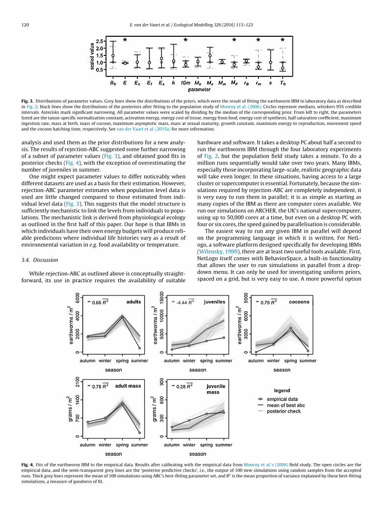

120 E. van der Vaart et al. / Ecological Modelling 326 (2016) 113–123

Fig. 3. Distributions of parameter values. Grey lines show the distributions of the priors, which were the result of fitting the earthworm IBM to laboratory data as describedin Fig. 2; black lines show the distributions of the posteriors after fitting to the population study of Monroy et al. (2006). Circles represent medians, whiskers 95% credibleintervals. Asterisks mark significant narrowing. All parameter values were scaled by dividing by the median of the corresponding prior. From left to right, the parametersl f tissui sexuaa e info

asopn

druvslawae

3

f

Fers

isted are the taxon-specific normalisation constant, activation energy, energy cost ongestion rate, mass at birth, mass of cocoon, maximum asymptotic mass, mass atnd the cocoon hatching time, respectively. See van der Vaart et al. (2015a) for mor

nalysis and used them as the prior distributions for a new analy-is. The results of rejection-ABC suggested some further narrowingf a subset of parameter values (Fig. 3), and obtained good fits inosterior checks (Fig. 4), with the exception of overestimating theumber of juveniles in summer.

One might expect parameter values to differ noticeably whenifferent datasets are used as a basis for their estimation. However,ejection-ABC parameter estimates when population level data issed are little changed compared to those estimated from indi-idual level data (Fig. 3). This suggests that the model structure isufficiently mechanistic to link the levels from individuals to popu-ations. The mechanistic link is derived from physiological ecologys outlined in the first half of this paper. Our hope is that IBMs inhich individuals have their own energy budgets will produce reli-

ble predictions where individual life histories vary as a result ofnvironmental variation in e.g. food availability or temperature.

.4. Discussion

While rejection-ABC as outlined above is conceptually straight-orward, its use in practice requires the availability of suitable

ig. 4. Fits of the earthworm IBM to the empirical data. Results after calibrating with thmpirical data, and the semi-transparent grey lines are the ‘posterior predictive checks’uns. Thick grey lines represent the mean of 100 simulations using ABC’s best-fitting paraimulations, a measure of goodness of fit.

e, energy from food, energy cost of synthesis, half saturation coefficient, maximuml maturity, growth constant, maximum energy to reproduction, movement speedrmation.

hardware and software. It takes a desktop PC about half a second torun the earthworm IBM through the four laboratory experimentsof Fig. 2, but the population field study takes a minute. To do amillion runs sequentially would take over two years. Many IBMs,especially those incorporating large-scale, realistic geographic datawill take even longer. In these situations, having access to a largecluster or supercomputer is essential. Fortunately, because the sim-ulations required by rejection-ABC are completely independent, itis very easy to run them in parallel; it is as simple as starting asmany copies of the IBM as there are computer cores available. Werun our simulations on ARCHER, the UK’s national supercomputer,using up to 50,000 cores at a time, but even on a desktop PC withfour or six cores, the speed gained by parallelisation is considerable.

The easiest way to run any given IBM in parallel will dependon the programming language in which it is written. For NetL-ogo, a software platform designed specifically for developing IBMs(Wilensky, 1999), there are at least two useful tools available. First,

NetLogo itself comes with BehaviorSpace, a built-in functionalitythat allows the user to run simulations in parallel from a drop-down menu. It can only be used for investigating uniform priors,spaced on a grid, but is very easy to use. A more powerful option

e empirical data from Monroy et al.’s (2006) field study. The open circles are the, i.e., the output of 100 new simulations using random samples from the acceptedmeter set, and R2 is the mean proportion of variance explained by these best-fitting

ical M

ift2r

resdSfmfi

aiSAsmAa‘osrmcilI

dstdaetabaT(oc

mAgAFiisytsbeibSIm

Resource Council [grant number NE/K006282/1, awarded to RM

E. van der Vaart et al. / Ecolog

s to use R, statistical software that, like NetLogo, is freely availableor all operating systems. R comes with many built-in distributionso draw priors from, and the packages RNetLogo (Thiele et al., 2012,014) and parallel together provide a means of performing NetLogouns in parallel.

The rejection-ABC analysis – Steps 3 and 4 of our rejection-ABCecipe above – can also be handled well by R. The R package abc, forxample, takes empirical data, a spreadsheet of priors and a spread-heet of results as its inputs, and produces as outputs the posterioristributions of Step 5 as well as the cross-validation diagnostics oftep 7. Other relevant R packages are listed by Thiele et al. (2014). Auture objective of ours is to release an R package which will auto-

ate the rejection-ABC process for NetLogo models from start tonish; a beta version is available upon request.

There are two common ways in which the basic rejection-ABClgorithm introduced in this paper is sometimes modified. First,t may be possible to sample a model’s priors more efficiently intep 3, using either MCMC-ABC (Marjoram et al., 2003) or SMC-BC (Sisson et al., 2007; Toni et al., 2009). MCMC-ABC bases eachubsequent run of the model on the previous one, and graduallyoves towards an estimate of the full posterior distribution. SMC-BC starts a set of simulations in parallel, sampling randomly from

model’s priors, but then gradually lowers the acceptance rate,zooming in’ towards the posterior distributions sought. Both meth-ds can potentially reduce the number of simulations requiredignificantly, but they may be harder to parallelise than basicejection-ABC. In addition, they may require more work to opti-ise: Defining how to move towards the best-fitting parameters

an be difficult, and if done incorrectly, algorithms may “get stuck”n the wrong areas of the parameter space. However, SMC-ABC isess vulnerable to these problems, and may be worth trying withBMs; Thiele et al. (2014) provide some introductory examples.

Improvements to the estimation of the posterior parameteristributions in Step 5 may also be possible. Known as “regres-ion methods” (Beaumont et al., 2002; Blum and Franc ois, 2010),hese techniques correct for the mismatch between the empiricalata and the model outputs in the accepted runs. Inevitably, someccepted runs are going to be closer to the empirical data than oth-rs, but in basic rejection-ABC, all these runs contribute equallyo the estimate of the posterior distributions. Regression methodsttempt to correct for this anomaly by analysing the relationshipetween the parameter values and the summary statistics in theccepted runs, and then correcting parameter values accordingly.he abc package implements various ways of doing this correctionCsillery et al., 2012), but may produce unreliable results if somef the empirical data lies far outside the range of model outputs, asan happen with IBMs.

Our hope in providing this introduction to ABC is to persuadeore ecological modellers to try it. Although the literature onBC is large and growing, it is still mainly applied to populationenetics problems. This means that it is still uncertain whetherBC’s existing conventions and innovations are optimal for IBMs.or instance, choosing appropriate summary statistics is a fieldn its own right—if the available empirical data is summarisedncorrectly, ABC’s posteriors may be biased, or require many moreimulations to get right (Blum et al., 2013); no general strategy canet be advocated for IBMs. Other questions include whether ABC’sypical distance measure (Eq. (4)) is the best choice for the timeeries data sometimes available in ecological applications, and howest to handle stochasticity. When we do simulation runs, we tryach parameter combination once, but for some models, averag-ng over multiple runs with the same parameter values might be

etter. Finally, whether advanced techniques such as MCMC-ABC,MC-ABC and the “regression correction” will prove workable withBMs in practice is yet to be investigated. IBMs often have many

ore parameters than typical population genetics models, and

odelling 326 (2016) 113–123 121

different kinds of dependencies between them—only by tryingthings out, with lots of different IBMs, can general strategies bedeveloped.

4. Conclusion

Science is a method of acquiring knowledge, and IBMs can beused to represent existing knowledge in ways that can be used topredict what will happen to individuals and populations in definedlandscapes. Physiological ecology contributes the knowledge ofhow individuals acquire and expend energy, while behaviouralecology covers the factors that affect foraging, competition andsocial coexistence. Integrating these insights into IBMs allows usto link the levels from individuals to populations better than hasbeen possible before. Even so, open questions remain. For example,at the individual level, there are still controversies about how ani-mals distribute energy between physiological processes, and whatthey do when there is energy shortfall. At the population level, weare only just beginning to integrate social structures like dominancehierarchies into practical simulation models.

Thus, building realistic IBMs still requires expert judgement,and extensive testing against empirical data. Approximate BayesianComputation, or ABC, is one possible approach to making this pro-cess more quantitative and transparent. Whereas the current stateof the art, ‘pattern-oriented modelling’, or POM, is essentially a ver-bal protocol, ABC offers a statistically rigorous approach to modelfitting and model comparison. However, ABC is fully compatiblewith the basic philosophy behind POM: That multiple empiricalpatterns, at multiple levels of organisation, should be used to buildflexible, mechanistic models, that truly capture the fundamentalaspects of the species and situations under consideration.

Although there are some challenges in implementing ABC forIBMs – most notably, the computing power required to evaluatemodels with long running times – the promise is considerable. ABCprovides approximate posterior distributions of a model’s param-eters given data. As illustrated by our example, these posteriorscan then be used as priors for further studies, and they can revealwhich parameters are correlated or underconstrained. They canalso be used to show the uncertainties that exist in a model’s futurepredictions. Equally importantly, the power of ABC goes beyondparameter estimation–it can also be used to compare structurallydifferent models, while automatically compensating for differencesin model complexity.

Finally, we believe that perhaps one of the greatest advantagesof ABC lies in its unifying language. Current efforts to parametriseIBMs, and to quantify their uncertainties, are often highly modeldependent, with different types of results and plots provided indifferent studies. In contrast, ABC offers a set of conventional waysto report priors, posteriors, credible intervals and Bayes factors, andto do posterior checks and cross-validation and to calculate cover-age. This should make model-fitting procedures more transparent.In addition, a basic understanding of ABC offers an entry point tothe more sophisticated model-fitting alternatives that are avail-able in the statistics literature. In sum, we believe ABC has much tooffer when it comes to building, calibrating and evaluating realisticIBMs.

Acknowledgments

This work was supported by the Natural Environmental

Sibly, M Beaumont, A Meade, PJ van Leeuwen and NK Nichols].This work used the ARCHER UK National Supercomputing Service(http://www.archer.ac.uk). We are very grateful to Volker Grimmand two anonymous referees for constructive comments.

1 ical M

R

B

B

B

B

B

B

B

C

C

C

D

D

D

E

G

G

G

G

G

G

G

G

H

H

H

H

H

H

J

K

K

KK

K

K

22 E. van der Vaart et al. / Ecolog

eferences

eaumont, M.A., 2010. Approximate Bayesian computation in evolution and ecology.Annu. Rev. Ecol., Evol. Syst. 41, 379–406.

eaumont, M.A., Zhang, W., Balding, D.J., 2002. Approximate Bayesian computationin population genetics. Genetics 162, 2025–2035.

egon, M., Townsend, C.R., Harper, J.L., 2006. Ecology: From Individuals to Ecosys-tems, fourth ed. Blackwell Publishing, Malden, MA.

ertorelle, G., Benazzo, A., Mona, S., 2010. ABC as a flexible framework to esti-mate demography over space and time: some cons, many pros. Mol. Ecol. 19,2609–2625.

lum, M.G.B., Francois, O., 2010. Non-linear regression models for approximateBayesian computation. Stat. Comput. 20, 63–73.

lum, M.G.B., Nunes, M.A., Prangle, D., Sisson, S.A., 2013. A comparative review ofdimension reduction methods in approximate Bayesian computation. Stat. Sci.28, 189–208.

rown, J.H., Sibly, R.M., 2012. The metabolic theory of ecology and its central equa-tion. In: Sibly, R.M., Brown, J.H., Kodric-Brown, A. (Eds.), Metabolic Ecology: AScaling Approach. Wiley-Blackwell, Oxford, pp. 21–33.

lauss, M., Schwarm, A., Ortmann, S., Streich, W.J., Hummel, J., 2007. A case of non-scaling in mammalian physiology? Body size, digestive capacity, food intake,and ingesta passage in mammalian herbivores. Comp. Biochem. Physiol., A: Mol.Integr. Physiol. 148, 249–265.

silléry, K., Blum, M.G.B., Gaggiotti, O.E., Franc ois, O., 2010. Approximate Bayesiancomputation (ABC) in practice. Trends Ecol. Evol. 25, 410–418.

sillery, K., Franc ois, O., Blum, M.G.B., 2012. abc: An R package for approximateBayesian computation (ABC). Methods Ecol. Evol. 3, 475–479.

alkvist, T., Sibly, R.M., Topping, C.J., 2011. How predation and landscape fragmen-tation affect vole population dynamics. PLoS ONE 6, e22834.

avies, N.B., Krebs, J.R., West, S.A., 2012. An Introduction to Behavioural Ecology,fourth ed. Wiley-Blackwell, Oxford, UK.

eAngelis, D.L., Mooij, W.M., 2005. Individual-based modeling of ecological andevolutionary processes. Annu. Rev. Ecol., Evol. Syst. 36, 147–168.

vans, M.R., Bithell, M., Cornell, S.J., Dall, S.R.X., Diaz, S., Emmott, S., Ernande, B.,Grimm, V., Hodgson, D.J., Lewis, S.L., Mace, G.M., Morecroft, M., Moustakas, A.,Murphy, E., Newbold, T., Norris, K.J., Petchey, O., Smith, M., Travis, J.M.J., Benton,T.G., 2013. Predictive systems ecology. Proc. R. Soc. B: Biol. Sci. 280, 20131452.

alic, N., Forbes, V., 2014. Ecological models in ecotoxicology and ecological riskassessment: an introduction to the special section. Environ. Toxicol. Chem. 33,1446–1448.

lazier, D.S., 2005. Beyond the ‘3/4-power law’: variation in the intra- and interspe-cific scaling of metabolic rate in animals. Biol. Rev. 80, 611–662.

lazier, D.S., 2008. Resource allocation patterns. In: Rauw, W.M. (Ed.), Resource Allo-cation Theory Applied to Farm Animal Production. CABI Publishing, Wallingford,UK, pp. 22–43.

osler, A.G., Greenwood, J.J.D., Perrins, C., 1995. Predation risk and the cost of beingfat. Nature 377, 621–623.

rimm, V., Railsback, S.F., 2005. Individual-based Modeling and Ecology. PrincetonUniversity Press, Princeton, NJ.

rimm, V., Railsback, S.F., 2012. Pattern-oriented modelling: a ‘multi-scope’ for pre-dictive systems ecology. Philos. Trans. R. Soc. B: Biol. Sci. 367, 298–310.

unadi, B., Blount, C., Edwards, C.A., 2002. The growth and fecundity of Eisenia fetida(Savigny) in cattle solids pre-composted for different periods. Pedobiologia 46,15–23.

unadi, B., Edwards, C.A., 2003. The effects of multiple applications of differentorganic wastes on the growth, fecundity and survival of Eisenia fetida (Savigny)(Lumbricidae). Pedobiologia 47, 321–329.

artig, F., Calabrese, J.M., Reineking, B., Wiegand, T., Huth, A., 2011. Statistical infer-ence for stochastic simulation models—theory and application. Ecol. Lett. 14,816–827.

artig, F., Dislich, C., Wiegand, T., Huth, A., 2014. Technical note: approximateBayesian parameterization of a process-based tropical forest model. Biogeo-sciences 11, 1261–1272.

artman, K.J., Kitchell, J.F., 2008. Bioenergetics modeling: progress since the 1992symposium. Trans. Am. Fish. Soc. 137, 216–223.

endriks, A.J., 1999. Allometric scaling of rate, age and density parameters in eco-logical models. Oikos 86, 293–310.

olling, C.S., 1959. The components of predation as revealed by a study of small-mammal predation of the European pine sawfly. Can. Entomol. 91, 293–320.

ou, C., 2014. Increasing energetic cost of biosynthesis during growth makes refeed-ing deleterious. Am. Natur. 184, 233–247.

ohnston, A.S.A., Hodson, M.E., Thorbek, P., Alvarez, T., Sibly, R.M., 2014. An energybudget agent-based model of earthworm populations and its application tostudy the effects of pesticides. Ecol. Modell. 280, 5–17.

arasov, W.H., Martinez del Rio, C., 2007. Physiological Ecology. Princeton UniversityPress, Princeton, NJ and Oxford, UK.

aspari, M., 2012. Stoiciometry. In: Sibly, R.M., Brown, J.H., Kodric-Brown, A. (Eds.),Metabolic Ecology: A Scaling Approach. Wiley-Blackwell, Oxford, UK, pp. 14–47.

ass, R.E., Raftery, A.E., 1995. Bayes factors. J. Am. Stat. Assoc. 90, 773–795.erkhoff, A.J., 2012. Modeling metazoan growth and ontogeny. In: Sibly, R.M., Brown,

J.H., Kodric-Brown, A. (Eds.), Metabolic Ecology: A Scaling Approach. Wiley-

Blackwell, Oxford, UK.

ooijman, S.A.L.M., 2010. Dynamic Energy Budget Theory, third ed. Cambridge Uni-versity Press, Cambridge, UK.

rebs, C.J., 2009. Ecology, sixth ed. Benjamin Cummings, San Francisco, CA.

odelling 326 (2016) 113–123

Kulakowska, K.A., Kulakowski, T.M., Inglis, I.R., Smith, G.C., Haynes, P.J., Prosser, P.,Thorbek, P., Sibly, R.M., 2014. Using an individual-based model to select amongalternative foraging strategies of woodpigeons: Data support a memory-basedmodel with a flocking mechanism. Ecol. Modell. 280, 89–101.

Lind, J., Jakobsson, S., Kullberg, C., 2010. Impaired predator evasion in the life historyof birds: behavioral and physiological adaptations to reduced flight ability. In:Thompson, C.F. (Ed.), Current Ornithology, vol. 17. Springer, New York, pp. 1–30.

Lindstedt, S.L., Schaeffer, P.J., 2002. Use of allometry in predicting anatomical andphysiological parameters of mammals. Lab. Anim. 36, 1–19.

Liu, C., Sibly, R.M., Grimm, V., Thorbek, P., 2013. Linking pesticide exposure and spa-tial dynamics: an individual-based model of wood mouse (Apodemus sylvaticus)populations in agricultural landscapes. Ecol. Modell. 248, 92–102.

Marjoram, P., Molitor, J., Plagnol, V., Tavaré, S., 2003. Markov chain Monte Carlowithout likelihoods. Proc. Natl. Acad. Sci. U.S.A. 100, 15238–15324.

Martin, B.T., Jager, T., Nisbet, R.M., Preuss, T.G., Grimm, V., 2013. Predicting popula-tion dynamics from the properties of individuals: a cross-level test of dynamicenergy budget theory. Am. Natur. 181, 506–519.

Martin, B.T., Zimmer, E.I., Grimm, V., Jager, T., 2012. Dynamic energy budget theorymeets individual-based modelling: a generic and accessible implementation.Methods Ecol. Evol. 3, 445–449.

Martínez, I., Wiegand, T., Camarero, J.J., Batllori, E., Gutiérrez, E., 2011. Disentan-gling the formation of contrasting tree-line physiognomies combining modelselection and Bayesian parameterization for simulation models. Am. Natur. 177,E136–E152.

Monroy, F., Aira, M., Domínguez, J., Velando, A., 2006. Seasonal population dynamicsof Eisenia fetida (Savigny, 1826) (Oligochaeta, Lumbricidae) in the field. ComptesRendus Biol. 329, 912–915.

Moses, M.E., Hou, C., Woodruff, W.H., West, G.B., Nekola, J.C., Zuo, W., Brown, J.H.,2008. Revisiting a model of ontogenetic growth: estimating model parametersfrom theory and data. Am. Natur. 171, 632–645.

Nabe-Nielsen, J., Sibly, R.M., Forchhammer, M.C., Forbes, V.E., Topping, C.J., 2010.The efects of landscape modifications on the long-term persistence of animalpopulations. PLoS ONE 5, e8932.

Nabe-Nielsen, J., Sibly, R.M., Tougaard, J., Teilmann, J., Sveegaard, S., 2014. Effects ofnoise and by-catch on a Danish harbour porpoise population. Ecol. Modell. 272,242–251.

Peters, R.H., 1983. The Ecological Implications of Body Size. Cambridge UniversityPress, Cambridge, UK.

Petit, O., Gautrais, J., Leca, J.B., Theraulaz, G., Deneubourg, J.-L., 2009. Collective deci-sion making in white-faced capuchin monkeys. Proc. R. Soc. B: Biol. Sci. 1672,3495–3503.

Pond, C.M., 1978. Morphological aspects and ecological and mechanical conse-quences of fat deposition in wild vertebrates. Ann. Rev. Ecol. Syst. 9, 519–570.

Prangle, D., Blum, M.G.B., Popovic, G., Sisson, S.A., 2013. Diagnostic tools for approx-imate Bayesian computation using the coverage property. Aust. N. Z. J. Stat. 56,309–329.

Price, C.A., Weitz, J.S., Savage, V.M., Stegen, J., Clarke, A., Coomes, D.A., Dodds, P.S.,Etienne, R.S., Kerkhoff, A.J., McCulloh, K., Niklas, K.J., Olff, H., Swenson, N.G., 2012.Testing the metabolic theory of ecology. Ecol. Lett. 15, 1465–1474.

Pritchard, J.K., Seielstad, M.T., Perez-Lezaun, A., Feldman, M.W., 1999. Populationgrowth of human Y chromosomes: a study of Y chromosome microsatellites.Mol. Biol. Evol. 16, 1791–1798.

Reinecke, A.J., Viljoen, S.A., 1990. The influence of feeding patterns on growth andreproduction of the vermicomposting earthworm Eisenia fetida (Oligochaeta).Biol. Fertil. Soils 10, 184–187.

Ricklefs, R.E., Miller, G.L., 2000. Ecology, fourth ed. W.H. Freeman and Co., New York,NY.

Sibly, R.M., 2002. Life history theory. In: Pagel, M. (Ed.), Encyclopedia of Evolution.Oxford University Press, Oxford, pp. 623–627.

Sibly, R.M., Calow, P., 1986. Physiological Ecology of Animals. Blackwell ScientificPublications, Oxford, UK.

Sibly, R.M., Grimm, V., Martin, B.T., Johnston, A.S.A., Kulakowska, K., Topping, C.J.,Calow, P., Nabe-Nielsen, J., Thorbek, P., DeAngelis, D.L., 2013. Representing theacquisition and use of energy by individuals in agent-based models of animalpopulations. Methods Ecol. Evol. 4, 151–161.

Sih, A., Cote, J., Evans, M., Fogarty, S., Pruitt, J., 2012. Ecological implications ofbehavioural syndromes. Ecol. Lett. 15, 278–289.

Simpson, S.J., Sibly, R.M., Lee, K.P., Behmer, S.T., Raubenheimer, D., 2004. Optimal for-aging when regulating intake of multiple nutrients. Anim. Behav. 68, 1299–1311.

Sinclair, A.R.E., 1989. Population regulation in animals. In: Cherrett, J.M. (Ed.), Eco-logical Concepts. Blackwell Scientific, Oxford, pp. 197–241.

Sisson, S.A., Fan, Y., Tanaka, M.A., 2007. Sequential Monte Carlo without likelihoods.Proc. Natl. Acad. Sci. U.S.A. 104, 1760–1765.

Stearns, S.C., 1992. The Evolution of Life Histories. Oxford University Press, Oxford,UK.

Stillman, R.A., Goss-Custard, J.D., 2010. Individual-based ecology of coastal birds.Biol. Rev. 85, 413–434.

Stillman, R.A., Railsback, S.F., Giske, J., Berger, U., Grimm, V., 2015. Making predictionsin a changing world: the benefits of individual-based ecology. BioScience 65,140–150.

Tavaré, S., Balding, D.J., Griffiths, R.C., Donnelly, P., 1997. Inferring coalescence times

from DNA sequence data. Genetics 145, 505–518.

Thiele, J.C., Kurth, W., Grimm, V., 2012. RNetLogo: an R package for running andexploring individual-based models implemented in NetLogo. Methods Ecol.Evol. 3, 480–483.

ical M

T

T

T

v

Wilensky, U., 1999. NetLogo. Center for Connected Learning and Computer-BasedModeling, Northwestern University, Evanston, IL, 〈http://ccl.northwestern.edu/netlogo/〉.

E. van der Vaart et al. / Ecolog

hiele, J.C., Kurth, W., Grimm, V., 2014. Facilitating parameter estimation and sensi-tivity analysis of agent-based models: a cookbook using NetLogo and R. J. Artif.Soc. Soc. Simul. 17, 11.

oni, T., Welch, D., Strelkowa, N., Ipsen, A., Stumpf, M.P.H., 2009. ApproximateBayesian computation scheme for parameter inference and model selection indynamical systems. J. R. Soc. Interf. 6, 187–202.

opping, C.J., Dalkvist, T., Grimm, V., 2012. Post-hoc pattern-oriented testing and

tuning of an existing large model: Lessons from the field vole. PLoS ONE 7,e45872.

an der Vaart, E., Beaumont, M.A., Johnston, A., Sibly, R.M., 2015a. Calibration andevaluation of individual-based models using approximate Bayesian computa-tion. Ecol. Modell. 312, 182–190.

odelling 326 (2016) 113–123 123

van der Vaart, E., Johnston, A., Sibly, R.M., 2015b. Linking Levels—Runs. Figshare,1494757, doi: http://dx.doi.org/10.6084/m9.figshare.

van der Vaart, E., Johnston, A.S.A., Sibly, R.M., 2015c. Linking Levels—Code. Figshare,1494754, doi: http://dx.doi.org/10.6084/m9.figshare.

Witter, M.S., Cuthill, I.C., 1993. The ecological costs of avian fat storage. Philos. Trans.R. Soc. London Ser. B: Biol. Sci. 340, 73–92.