predicting ground-level scene layout from aerial imagery
TRANSCRIPT
Predicting Ground-Level Scene Layout from Aerial Imagery
Menghua Zhai
Zachary Bessinger
Scott Workman
Nathan Jacobs
Computer Science, University of Kentucky
Abstract
We introduce a novel strategy for learning to extract se-
mantically meaningful features from aerial imagery. In-
stead of manually labeling the aerial imagery, we propose
to predict (noisy) semantic features automatically extracted
from co-located ground imagery. Our network architecture
takes an aerial image as input, extracts features using a
convolutional neural network, and then applies an adaptive
transformation to map these features into the ground-level
perspective. We use an end-to-end learning approach to
minimize the difference between the semantic segmentation
extracted directly from the ground image and the semantic
segmentation predicted solely based on the aerial image.
We show that a model learned using this strategy, with no
additional training, is already capable of rough semantic
labeling of aerial imagery. Furthermore, we demonstrate
that by finetuning this model we can achieve more accu-
rate semantic segmentation than two baseline initialization
strategies. We use our network to address the task of esti-
mating the geolocation and geo-orientation of a ground im-
age. Finally, we show how features extracted from an aerial
image can be used to hallucinate a plausible ground-level
panorama.
1. Introduction
Learning-based methods for pixel-level labeling of aerial
imagery have long relied on manually annotated training
data. Unfortunately, such data is expensive to create. Fur-
thermore, its value is limited because a method trained on
one dataset will typically not perform well when applied
to another source of aerial imagery. The difficulty in ob-
taining datasets of sufficient scale for all modalities has
hampered progress in applying deep learning techniques
to aerial imagery. There have been a few notable excep-
tions [22, 24], but these have all used fairly coarse grained
semantic classes, covered a small spatial area, and are lim-
ited to modalities in which human annotators are able to
manually assign labels.
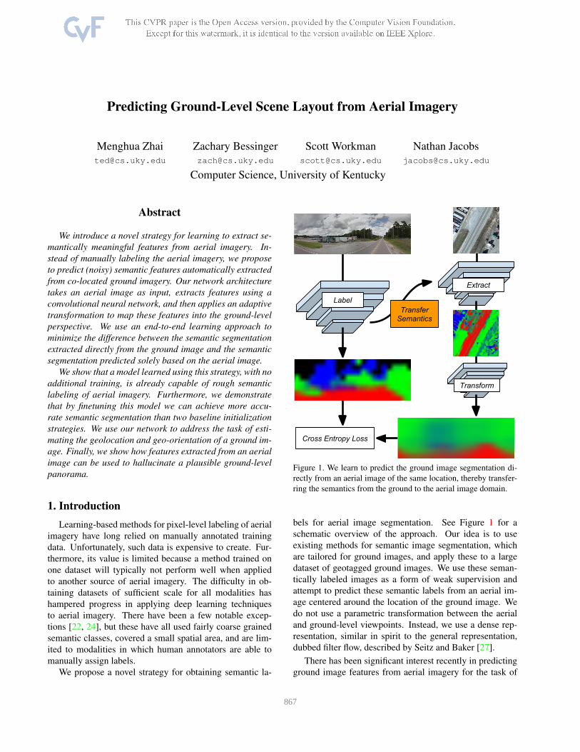
We propose a novel strategy for obtaining semantic la-
Cross Entropy Loss
Label
Extract
Transform
TransferSemantics
Figure 1. We learn to predict the ground image segmentation di-
rectly from an aerial image of the same location, thereby transfer-
ring the semantics from the ground to the aerial image domain.
bels for aerial image segmentation. See Figure 1 for a
schematic overview of the approach. Our idea is to use
existing methods for semantic image segmentation, which
are tailored for ground images, and apply these to a large
dataset of geotagged ground images. We use these seman-
tically labeled images as a form of weak supervision and
attempt to predict these semantic labels from an aerial im-
age centered around the location of the ground image. We
do not use a parametric transformation between the aerial
and ground-level viewpoints. Instead, we use a dense rep-
resentation, similar in spirit to the general representation,
dubbed filter flow, described by Seitz and Baker [27].
There has been significant interest recently in predicting
ground image features from aerial imagery for the task of
1867
ground image geolocalization [34]. Our work is unique in
that it is the first to attempt to predict a dense pixel-level seg-
mentation of the ground image. We demonstrate the value
of this approach in several ways.
Main Contributions: The main contributions of this
work are: (1) a novel convolutional neural network (CNN)
architecture that relates the appearance of an aerial image to
the semantic layout of a ground image of the same location,
(2) demonstrating the value of our training strategy for pre-
training a CNN to understand aerial imagery, (3) extensions
of the proposed technique to the tasks of ground image lo-
calization, orientation estimation, and synthesis, and (4) an
extensive evaluation of each of these techniques on large,
real-wold datasets. Together these represent an important
step in enabling deep learning techniques to be extended to
the domain of aerial image understanding.
2. Related Work
Learning Viewpoint Transformations Many methods
have been proposed to represent the relationship between
the appearance of two viewpoints. Seitz and Baker [27]
model image transformations using a space-variant linear
filter, similar to a convolution but varying per-pixel. They
highlight that a linear transformation of a vectorized rep-
resentation of all the pixels in an image is very general;
it can represent all standard parametric transformations,
such as similarity, affine, perspective, and more. More re-
cently, Jaderberg et al. [13] describe an end-to-end learn-
able module for neural networks, the spatial transformer,
which allows explicit spatial transformations (e.g., scaling,
cropping, rotation, non-rigid deformation) of feature maps
within the network that are conditioned on individual data
samples. Practically, including a spatial transformer allows
a network to select regions of interest from an input and
transform them to a canonical pose. Similarly, Tinghui
et al. [35] address the problem of novel view synthesis.
They observe that the visual appearance of different views
is highly correlated and propose a CNN architecture for es-
timating appearance flows, a representation of which pixels
in the input image can be used for reconstruction.
Relating Aerial and Ground-Level Viewpoints Several
methods have been recently proposed to jointly reason
about co-located aerial and ground image pairs. Luo et
al. [20] demonstrate that aerial imagery can aid in rec-
ognizing the visual content of a geotagged ground image.
Mattyus et al. [21] perform joint inference over monocular
aerial imagery and stereo ground images for fine-grained
road segmentation. Wegner et al. [31] build a map of street
trees. Given the horizon line and the camera intrinsics,
Ghouaiel and Lefevre [8] transform geotagged ground-level
panoramas to a top-down view to enable comparisons with
aerial imagery for the task of change detection. Recent work
on cross-view image geolocalization [18, 19, 33, 34] has
shown that convolutional neural networks are capable of ex-
tracting features from aerial imagery that can be matched
to features extracted from ground imagery. Vo et al. [30]
extend this line of work, demonstrating improved geolocal-
ization performance by applying an auxiliary loss function
to regress the ground-level camera orientation with respect
to the aerial image. To our knowledge, our work is the first
work to explore predicting the semantic layout of a ground
image from an aerial image.
Semantic Segmentation of Aerial/Satellite Imagery
There is a long tradition of using computer vision tech-
niques for aerial and satellite image understanding [11, 32,
4]. Historically these two domains were distinct. Satellite
imagery was typically lower-resolution, from a strictly top-
down view, and with a diversity of spectral bands. Aerial
imagery was typically higher-resolution, with a greater di-
versity of viewing angles, but with only RGB and NIR sen-
sors. Recently these two domains have converged; we will
use the term aerial imagery as we are primarily working
with high-resolution RGB imagery. However, our approach
could be applied to many types of aerial and satellite im-
agery. Kluckner et al. [17] address the task of semantic
segmentation using a random forest to combine color and
height information. More recent work has explored the use
of CNNs for aerial image understanding. Mnih and Hinton
propose a CNN for detecting roads in aerial imagery [22]
using GIS data as ground truth. They extend their approach
to handle omission noise and misregistration between the
imagery and the labels [23]. These approaches require ei-
ther extensive pixel-level manual annotation or existing GIS
data. Our work is the first to demonstrate the ability to trans-
fer a dense pixel-level labeling of ground imagery to aerial
imagery.
Visual Domain Adaptation Domain adaptation ad-
dresses the misalignment of source and target domains [7].
A significant amount of work has explored domain adap-
tation for visual recognition [25]. Jhuo et al. [14] propose
a low-rank reconstruction approach where the source fea-
tures are transformed to an intermediate representation in
which they can be linearly reconstructed by the target sam-
ples. Our work is most similar to that of Sun et al. [29], who
propose a method for transferring scene categorizations and
attributes from ground images to aerial imagery. Similar
to our approach, they learn a transformation matrix which
minimizes the distance between a source feature and the tar-
get feature. Our work differs in several ways: 1) we carry
out the linear transformation not only in the semantic di-
mensions but also in the spatial dimensions, 2) we constrain
868
256
1✕1✕289
interpolate to size 17 x 17 x channels
64128
512
aerial label
S
1✕1✕4
(i, j, y, x)
transformation matrix
aerial image
VGG16A
F
T
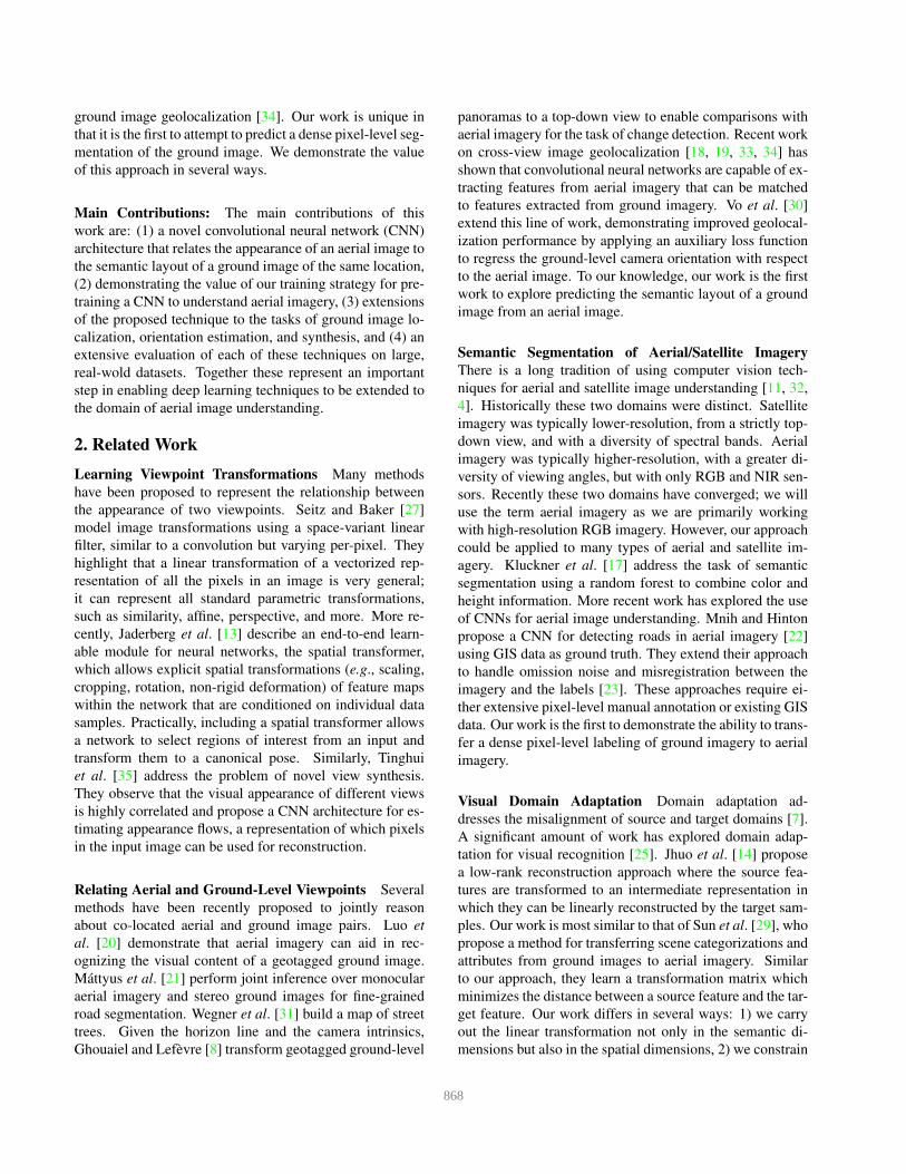
Figure 2. A visual overview of our network architecture. We extract features from an aerial image using the VGG16 architecture and
form a hypercolumn using the PixelNet approach. These features are processed by three networks that consist of 1 × 1 convolutions:
network A converts the hypercolumn into semantic features; network S extracts useful features from the aerial image for controlling the
transformation; and network F defines the transformation between viewpoints. The transformation, T , is applied to the aerial semantic
features to create a ground-level semantic labeling.
the transformation matrix such that the semantic meaning of
the source feature and the target feature remains the same,
3) our transformation matrix is input dependent, and 4) we
learn the transformation matrix as well as the source feature
at the same time, in an end-by-end manner, which simplifies
training.
3. Cross-view Supervised Training
We propose a novel training strategy for learning to ex-
tract useful features from aerial imagery. The idea is to pre-
dict the semantic scene layout, Lg , of a ground image, Ig ,
using only an aligned aerial image, Ia, from the same lo-
cation. This strategy leverages existing methods for ground
image understanding at training time, but does not require
any ground imagery at testing time.
We represent semantic scene layout, Lg , as a pixel-level
probability distribution over classes, such as road, vegeta-
tion, and building. We construct a training pair by collecting
a georegistered ground panorama and an aerial image of the
same location, orienting the panorama to the aerial image
(panoramas are originally aligned with the road direction),
and then extracting the semantic scene layout, Lg , of the
panorama using an off-the-shelf method [2] with four se-
mantic classes. We then use an end-to-end training strategy
to learn to extract pixel-level features from the aerial image
and transform them to the ground-level viewpoint.
3.1. Network Architecture
Our proposed network architecture is composed of four
modules. A convolutional neural network (CNN), La =
A(Ia; ΘA), is used to extract semantic labels from the aerial
imagery. Another CNN, S(Ia; ΘS), uses features extracted
from aerial imagery to help estimate the transformation
matrix, M = F (xr, yr, ic, jc, S(Ia; ΘS); ΘF ), based on
aerial image features and the pixel location in the respec-
tive images. Finally, we have a transformation module,
Lg′ = T (La,M), that converts from the aerial viewpoint
to the ground-level using the estimated transformation ma-
trix, M . There are many choices for these components, and
the remainder of this section describes the particular choices
we made for this study. See Figure 2 for a visual overview
of the architecture.
Aerial Image Feature Extraction For A(Ia; ΘA), we
use the VGG16 [28] base architecture and convert it
to a pixel-level labeling method using the PixelNet ap-
proach [3]. The core idea is to interpolate intermediate fea-
ture maps of the base network to a uniform size, then con-
catenate them along the channels dimension to form a hy-
percolumn. In our experiments, we form the hypercolumn
from conv-{12, 22, 33, 43} of the VGG16 network. The hy-
percolumn, which is now 256 × 256 × 960, is followed by
three 1 × 1 convolutional layers, with 512, 512, and 4 out-
put channels respectively. The first two 1 × 1 convolutions
have ReLU activations, the final is linear. We designate the
output of the final convolution as La = A(Ia; ΘA). The
output of this stage is transformed from a aerial viewpoint
to a ground viewpoint by the final stage of the network.
Cross-view Semantic Transformation We represent the
transformation between the aerial and ground-level view-
869
points as a linear operation applied channel-wise to La.
To transform from the ha × wa× 4 aerial label, La, to
the hg × wg× 4 ground label, Lg′ , we need to estimate a
hgwg × hawa row-stochastic matrix, M . Given M , the
transformation process is as follows: reshape the aerial la-
bel, La, into a hawa× 4 matrix, la; multiply it by M to
get lg′ ; then reshape lg′ to the size of the ground label, Lg ,
to form our estimate of the ground label, Lg′ . To account
for the expected layout of the scene, and to handle the sky
class (which is not visible from the aerial image), we carry
out the transformation on the logits of la, fa, and add a bias
term, b to get the logits of lg′ , fg′ : fg′ = Mfa + b.There are many ways of representing the transformation
matrix, M , in a neural network. The naıve approach is to
treat M as a matrix of learnable variables. However, this
approach has two downsides: (1) the transformation does
not depend on the content of the aerial image and (2) the
number of parameters scales quadratically with the number
of pixels in La and Lg .
We represent each element, Mrc, in the transformation
matrix, M , as the output of a neural network, F , which is
conditioned on the aerial image, Ia, and the location in the
input and output feature maps. More precisely, each ele-
ment Mrc = F (xr, yr, ic, jc, S(Ia; ΘS)), where (ic, jc) ∈[0, 1], is the aerial image pixel of the corresponding element,
(yr, xr) ∈ [0, 1] is the ground image pixel of the corre-
sponding element.
We now define the architecture of the transformation es-
timation neural network, F . The value of the transformation
matrix at location (r, c) is computed through a neural net-
work, F , followed by a softmax function to normalize the
impact of all pixels sampled from the aerial image:
Mrc = F (r, c, S(Ia; ΘS)) =eFr,c
∑c′ e
Fr,c′
,
where:
Fr,c = F (i, j, y, x, S(Ia; ΘS)) , and
i = ⌊c/wa⌋/ha, j = mod(c, wa)/wa,
y = ⌊r/wg⌋/hg, x = mod(r, wg)/wg.
The base network, F , is a multilayer perceptron, with ReLU
activation functions, that takes as input a 293-element vec-
tor. The network has three layers, with 128, 64, and 1 output
channels respectively (refer to the lower part of Figure 2).
The naıve approach can be considered a special case of this
representation where we ignore the aerial image and use a
one-hot encoding representation of rows and columns.
As described above, there are two main advantages of
our approach of representing the transformation matrix: a
reduction in the number of parameters when M is large
and the ability to adapt to different aerial image layouts.
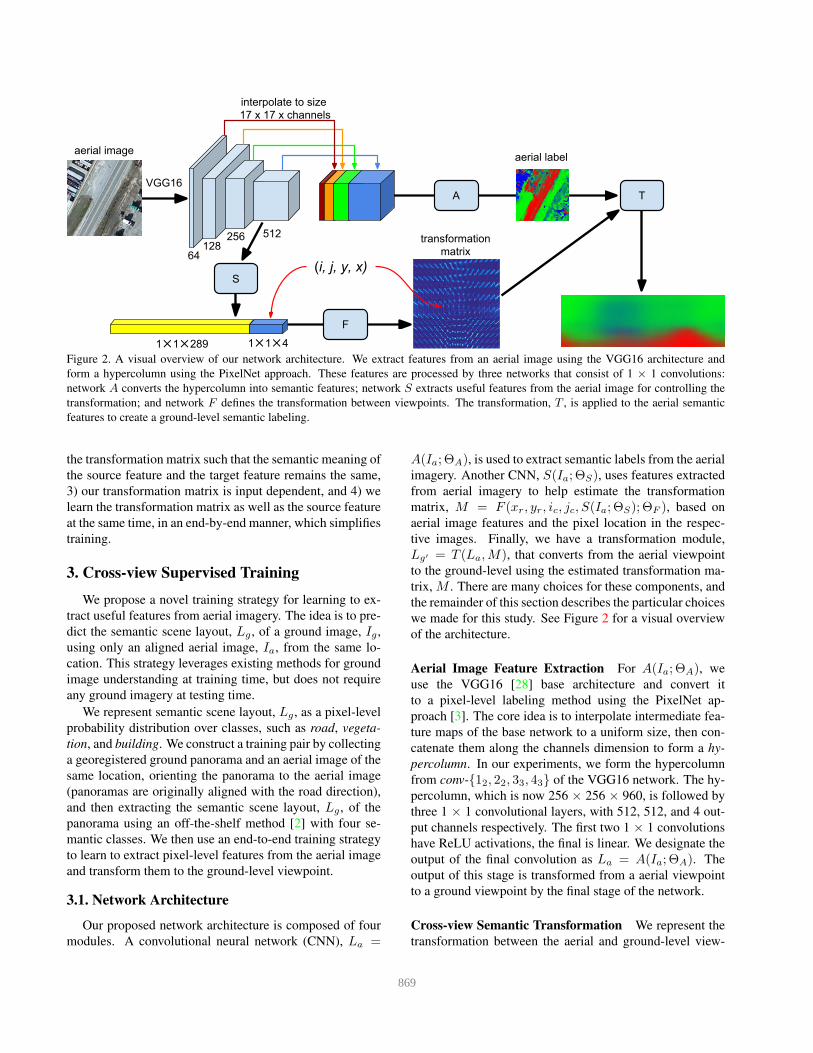
An additional benefit is that if we change the resolution of
resh
ape
(i, j)
(y, x)Transformation matrix elements of locations: { (i, j, y, x) | ∀i, j }
Figure 3. Visualization of the transformation matrix. (left) trans-
formation matrix, M ; (right-top) An alternative visualization, M ′,
of the transformation matrix. M ′ contains hg × wg cells (square
heat maps). Each cell, m′
yx, is reshaped to size ha × wa, from
one row of M that corresponds to locations, {(i, j, y, x) | ∀i, j}.
We also present the aerial image (overlapped with m′
yx) and the
ground image to illustrate how the hot spot of m′
yx corresponds to
the location, (y, x), on the ground image.
Figure 4. Examples of aligned aerial/ground image pairs from our
dataset. (row 1) In the aerial images, north is the up direction.
In the ground images, north is the central column. (row 2-4) Im-
age dependent receptive fields estimated by our algorithm as fol-
lows: 1) fix ground locations (y, x) (locations in squares); 2) select
all (i, j) (locations in contours) with high F (i, j, y, x, S(Ia; ΘS))values. Corresponding fields between the aerial image and the
ground image are shown in the same color.
our input and output feature maps it is easy to create a new
transformation matrix, M , without needing to resort to in-
terpolation. The transformation matrix learned by our al-
gorithm encodes pixel correspondences between the aerial
image and ground image (see Figure 3). We present more
examples of pixel correspondences in Figure 4.
3.2. Dataset
We collect our training and testing dataset from the
CVUSA dataset [34]. CVUSA contains approximately 1.5
870
million geotagged pairs of ground and aerial images from
across the United States. We use the Google Street View
panoramas of CVUSA as our ground images. For each
panorama, we also download an aerial image at zoom level
19 from Microsoft Bing Maps in the same location. We
filter out panoramas with no available corresponding aerial
imagery. Using the camera’s extrinsic information, we then
warp the panoramas to align with the aerial images. We
also crop the panoramas vertically to reduce the portion of
the sky and ground pixels. In total, we collected 35,532
image pairs for training and 8,884 image pairs for testing.
Some examples of aerial/ground image pairs in our dataset
are shown Figure 4.
3.3. Implementation Details
We implemented the proposed architecture using
Google’s TensorFlow framework [1]. We train our net-
works for 10 epochs with the Adam optimizer [16]. We
enable batch normalization [12] with decay 0.9 in all con-
volutional and fully-connected layers (except for the output
layers) to accelerate the training process. Our implementa-
tion is available at [6].
The training procedure is as follows: for a given cross-
view image pair, (Ia, Ig), we first compute the ground
semantic pixel label: Ig → Lg , using SegNet [2].
We then minimize the cross entropy between Lg and
T (A(Ia; ΘA); ΘT ) with respect to the model parameters,
ΘA and ΘT . The resulting architecture requires a signifi-
cant amount of memory to output the full final feature map,
which would normally result in very small batch sizes for
GPU training. Due to the PixelNet approach of using inter-
polation to scale the feature maps, we are able to perform
sparse training. Instead of outputting the full-size feature
map, we only extract a dense grid of points, the resulting
feature map is 17 × 17 × 4. Despite this, at testing time, we
can provide an aerial image and generate a full-resolution,
semantically meaningful feature map.
4. Evaluation and Applications
In this section, we will show that our network architec-
ture can be used in four different tasks: 1) weakly super-
vised semantic learning, 2) aerial imagery labeling, 3) ori-
entation regression and geocalibration, and 4) cross-view
image synthesis. Additional qualitative results and the com-
plete network structure used for cross-view image synthesis
can be found in our supplemental materials.
4.1. Weakly Supervised Learning
We trained our full network architecture (with randomly
initialized weights) to predict ground-level semantic label-
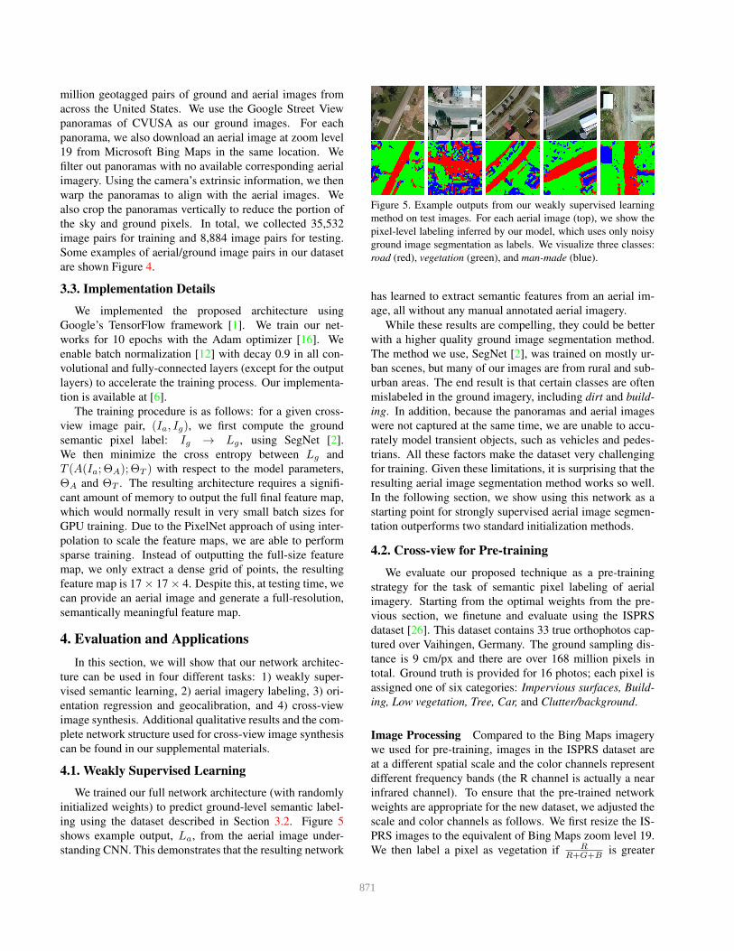
ing using the dataset described in Section 3.2. Figure 5
shows example output, La, from the aerial image under-
standing CNN. This demonstrates that the resulting network
Figure 5. Example outputs from our weakly supervised learning
method on test images. For each aerial image (top), we show the
pixel-level labeling inferred by our model, which uses only noisy
ground image segmentation as labels. We visualize three classes:
road (red), vegetation (green), and man-made (blue).
has learned to extract semantic features from an aerial im-
age, all without any manual annotated aerial imagery.
While these results are compelling, they could be better
with a higher quality ground image segmentation method.
The method we use, SegNet [2], was trained on mostly ur-
ban scenes, but many of our images are from rural and sub-
urban areas. The end result is that certain classes are often
mislabeled in the ground imagery, including dirt and build-
ing. In addition, because the panoramas and aerial images
were not captured at the same time, we are unable to accu-
rately model transient objects, such as vehicles and pedes-
trians. All these factors make the dataset very challenging
for training. Given these limitations, it is surprising that the
resulting aerial image segmentation method works so well.
In the following section, we show using this network as a
starting point for strongly supervised aerial image segmen-
tation outperforms two standard initialization methods.
4.2. Crossview for Pretraining
We evaluate our proposed technique as a pre-training
strategy for the task of semantic pixel labeling of aerial
imagery. Starting from the optimal weights from the pre-
vious section, we finetune and evaluate using the ISPRS
dataset [26]. This dataset contains 33 true orthophotos cap-
tured over Vaihingen, Germany. The ground sampling dis-
tance is 9 cm/px and there are over 168 million pixels in
total. Ground truth is provided for 16 photos; each pixel is
assigned one of six categories: Impervious surfaces, Build-
ing, Low vegetation, Tree, Car, and Clutter/background.
Image Processing Compared to the Bing Maps imagery
we used for pre-training, images in the ISPRS dataset are
at a different spatial scale and the color channels represent
different frequency bands (the R channel is actually a near
infrared channel). To ensure that the pre-trained network
weights are appropriate for the new dataset, we adjusted the
scale and color channels as follows. We first resize the IS-
PRS images to the equivalent of Bing Maps zoom level 19.
We then label a pixel as vegetation if RR+G+B
is greater
871
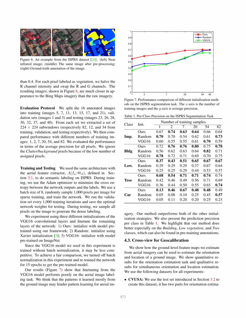
Figure 6. An example from the ISPRS dataset [26]. (left) Near
infrared image; (middle) The same image after pre-processing;
(right) Ground-truth annotation of the image.
than 0.4. For each pixel labeled as vegetation, we halve the
R channel intensity and swap the R and G channels. The
resulting images, shown in Figure 6, are much closer in ap-
pearance to the Bing Maps imagery than the raw imagery.
Evaluation Protocol We split the 16 annotated images
into training (images 5, 7, 11, 13, 15, 17, and 21), vali-
dation sets (images 1 and 3) and testing (images 23, 26, 28,
30, 32, 37, and 40). From each set we extracted a set of
224 × 224 subwindows (respectively 82, 12, and 34 from
training, validation, and testing respectively). We then com-
pared performance with different numbers of training im-
ages: 1, 2, 7, 20, 54, and 82. We evaluated the performance
in terms of the average precision for all pixels. We ignore
the Clutter/background pixels because of the low number of
assigned pixels.
Training and Testing We used the same architecture with
the aerial feature extractor, A(Ia; ΘA), defined in Sec-
tion 3.1, to do semantic labeling on ISPRS. During train-
ing, we use the Adam optimizer to minimize the cross en-
tropy between the network outputs and the labels. We use a
batch size of 8, randomly sample 1,000 pixels per image for
sparse training, and train the network. We run the valida-
tion set every 1,000 training iterations and save the optimal
network weights for testing. During testing, we sample all
pixels on the image to generate the dense labeling.
We experiment using three different initializations of the
VGG16 convolutional layers and finetune the remaining
layers of the network: 1) Ours: initialize with model pre-
trained using our framework; 2) Random: initialize using
Xavier initialization [9]; 3) VGG16: initialize with model
pre-trained on ImageNet.
Since the VGG16 model we used in this experiment is
trained without batch normalization, it may be less com-
petitive. To achieve a fair comparison, we turned off batch
normalization in this experiment and re-trained the network
for 15 epochs to get the pre-trained model.
Our results (Figure 7) show that finetuning from the
VGG16 model performs poorly on the aerial image label-
ing task. We think that the patterns it learned mostly from
the ground image may hinder pattern learning for aerial im-
1 2 7 20 54 820
0.1
0.2
0.3
0.4
0.5
0.6
0.7
0.8
0.9
1
Ours
Random
VGG16
Figure 7. Performance comparison of different initialization meth-
ods on the ISPRS segmentation task. The x-axis is the number of
training images and the y-axis is average precision.
Table 1. Per-Class Precision on the ISPRS Segmentation Task
Class Init.Number of training samples
1 2 7 20 54 82
Imp.
Ours 0.67 0.74 0.63 0.64 0.66 0.64
Random 0.70 0.70 0.54 0.62 0.61 0.73
VGG16 0.60 0.55 0.55 0.61 0.70 0.59
Bldg
Ours 0.72 0.76 0.76 0.80 0.75 0.78
Random 0.56 0.62 0.63 0.64 0.82 0.71
VGG16 0.78 0.72 0.71 0.69 0.70 0.75
Low.
Ours 0.37 0.43 0.51 0.65 0.67 0.67
Random 0.29 0.29 0.29 0.37 0.67 0.64
VGG16 0.25 0.25 0.29 0.44 0.53 0.57
Tree
Ours 0.68 0.54 0.71 0.71 0.74 0.74
Random 0.42 0.46 0.49 0.56 0.71 0.69
VGG16 0.36 0.44 0.50 0.55 0.65 0.74
Car
Ours 0.13 0.46 0.67 0.48 0.48 0.49
Random 0.05 0.08 0.10 0.25 0.45 0.57
VGG16 0.05 0.11 0.20 0.20 0.25 0.23
agery. Our method outperforms both of the other initial-
ization strategies. We also present the prediction precision
per class in Table 1. We highlight that our method does
better especially on the Building, Low vegetation, and Tree
classes, which can also be found in pre-training annotations.
4.3. Crossview for Geocalibration
We show how the ground-level feature maps we estimate
from aerial imagery can be used to estimate the orientation
and location of a ground image. We show quantitative re-
sults for the orientation estimation task and qualitative re-
sults for simultaneous orientation and location estimation.
We use the following datasets for all experiments:
• CVUSA: We use the test set introduced in Section 3.2 to
create this dataset; it has two parts for orientation estima-
872
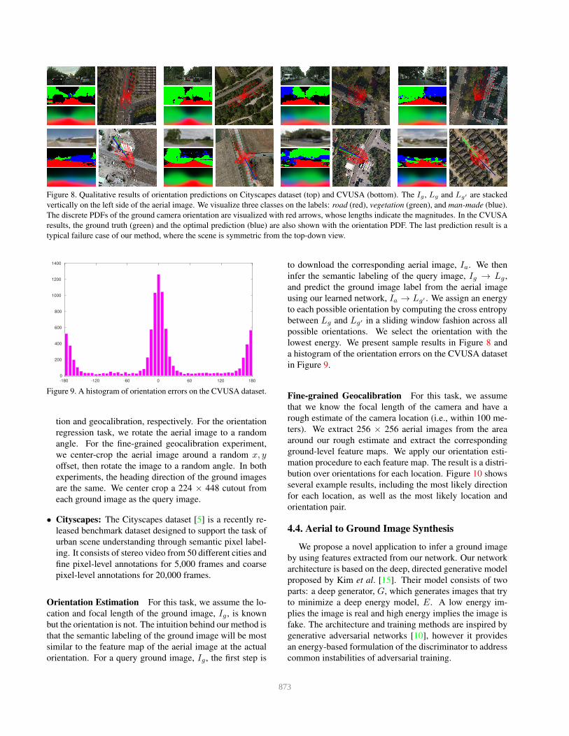
Figure 8. Qualitative results of orientation predictions on Cityscapes dataset (top) and CVUSA (bottom). The Ig , Lg and Lg′ are stacked
vertically on the left side of the aerial image. We visualize three classes on the labels: road (red), vegetation (green), and man-made (blue).
The discrete PDFs of the ground camera orientation are visualized with red arrows, whose lengths indicate the magnitudes. In the CVUSA
results, the ground truth (green) and the optimal prediction (blue) are also shown with the orientation PDF. The last prediction result is a
typical failure case of our method, where the scene is symmetric from the top-down view.
-180 -120 -60 0 60 120 180
0
200
400
600
800
1000
1200
1400
Figure 9. A histogram of orientation errors on the CVUSA dataset.
tion and geocalibration, respectively. For the orientation
regression task, we rotate the aerial image to a random
angle. For the fine-grained geocalibration experiment,
we center-crop the aerial image around a random x, yoffset, then rotate the image to a random angle. In both
experiments, the heading direction of the ground images
are the same. We center crop a 224 × 448 cutout from
each ground image as the query image.
• Cityscapes: The Cityscapes dataset [5] is a recently re-
leased benchmark dataset designed to support the task of
urban scene understanding through semantic pixel label-
ing. It consists of stereo video from 50 different cities and
fine pixel-level annotations for 5,000 frames and coarse
pixel-level annotations for 20,000 frames.
Orientation Estimation For this task, we assume the lo-
cation and focal length of the ground image, Ig , is known
but the orientation is not. The intuition behind our method is
that the semantic labeling of the ground image will be most
similar to the feature map of the aerial image at the actual
orientation. For a query ground image, Ig , the first step is
to download the corresponding aerial image, Ia. We then
infer the semantic labeling of the query image, Ig → Lg ,
and predict the ground image label from the aerial image
using our learned network, Ia → Lg′ . We assign an energy
to each possible orientation by computing the cross entropy
between Lg and Lg′ in a sliding window fashion across all
possible orientations. We select the orientation with the
lowest energy. We present sample results in Figure 8 and
a histogram of the orientation errors on the CVUSA dataset
in Figure 9.
Fine-grained Geocalibration For this task, we assume
that we know the focal length of the camera and have a
rough estimate of the camera location (i.e., within 100 me-
ters). We extract 256 × 256 aerial images from the area
around our rough estimate and extract the corresponding
ground-level feature maps. We apply our orientation esti-
mation procedure to each feature map. The result is a distri-
bution over orientations for each location. Figure 10 shows
several example results, including the most likely direction
for each location, as well as the most likely location and
orientation pair.
4.4. Aerial to Ground Image Synthesis
We propose a novel application to infer a ground image
by using features extracted from our network. Our network
architecture is based on the deep, directed generative model
proposed by Kim et al. [15]. Their model consists of two
parts: a deep generator, G, which generates images that try
to minimize a deep energy model, E. A low energy im-
plies the image is real and high energy implies the image is
fake. The architecture and training methods are inspired by
generative adversarial networks [10], however it provides
an energy-based formulation of the discriminator to address
common instabilities of adversarial training.
873
Figure 10. Fine-grained geocalibration results on CVUSA. (left) From top to bottom are the Ig , Lg , and Lg′ respectively. We visualize
three classes on the labels: road (red), vegetation (green), and man-made (blue). (right) Orientation flow map (red), where the arrow
direction indicates the optimal direction at that location and length indicates the magnitude. We also show the optimal prediction and the
ground-truth frustums in blue and green respectively.
Figure 11. Synthesized ground-level views. Each row shows an
aerial image (left), its corresponding ground-level panorama (top-
right), and predicted ground-level panorama (bottom-right).
We begin by extracting an 8 × 40 × 512 cross-view fea-
ture map, f , that has been learned to relate an aerial and
ground image pair. The generator is given f along with
random noise, z, as input. The generator outputs a 64 ×320 panorama, Ig , that represents the predicted ground im-
age. The cross-view feature, predicted panorama, and the
ground truth panorama, Ig , are input to the energy model.
Batch normalization [12] is applied in every layer of both
models, except for the final layers. ReLU activations are
used throughout the generator and Leaky ReLU, with leak
parameter α = 0.2, are used in the energy model. The mod-
els are updated in an alternating fashion, where the genera-
tor is updated twice for every update of the energy model.
Both the generator and energy model are optimized using
the Adam optimizer, with moment parameters β1 = 0.5and β2 = 0.999. We train using batch sizes of 32 for 30
epochs. A complete description of the architecture used in
this section is provided in our supplemental materials.
Example outputs generated by our network are shown in
Figure 11. Each row contains an aerial image (left), its re-
spective ground panorama (top-right), and our prediction of
the ground scene layout (bottom-right), which would ide-
ally be the same. The network has learned the most com-
mon features, such as roads and their orientations, as well
as trees and grass. However, it has difficulty hallucinating
buildings and the sky, which is likely caused by highly vari-
able appearance factors.
We note that the resolution of the synthesized ground-
level panoramas is much lower than the original panorama,
however adversarial generation of high-resolution images is
an active area of research. We expect that in the near future
we will be able to use our learned features in a similar man-
ner to generate full-resolution panoramas. Additionally, al-
gorithmic improvements to our ground image segmentation
method would provide more photo-realistic predictions.
5. Conclusion
We introduced a novel strategy for using labeled ground
images as a form of weak supervision for learning to un-
derstand aerial images. The key is to simultaneously learn
to extract features from the aerial image and learn to map
from the aerial to the ground image. We demonstrated that
by using this process we are able to automatically extract se-
mantically meaningful features from aerial imagery, refine
these to obtain more accurate pixel-level labeling of aerial
imagery, estimate the location and orientation of a ground
image, and synthesize novel ground-level views. The pro-
posed technique is equally applicable to other forms of im-
agery, including NIR, multispectral, and hyperspectral. For
future work, we plan to explore richer ground image anno-
tation methods to explore the limits of what is predictable
about a ground-level view from an aerial view.
Acknowledgements
We gratefully acknowledge the support of NSF CA-
REER grant (IIS-1553116), a Google Faculty Research
Award, and an AWS Research Education grant.
874
References
[1] M. Abadi, A. Agarwal, P. Barham, E. Brevdo, Z. Chen,
C. Citro, G. S. Corrado, A. Davis, J. Dean, M. Devin, et al.
Tensorflow: Large-scale machine learning on heterogeneous
distributed systems. arXiv preprint arXiv:1603.04467, 2016.
5
[2] V. Badrinarayanan, A. Kendall, and R. Cipolla. Segnet: A
deep convolutional encoder-decoder architecture for image
segmentation. arXiv preprint arXiv:1511.00561, 2015. 3, 5
[3] A. Bansal, X. Chen, B. Russell, A. Gupta, and D. Ramanan.
Pixelnet: Towards a General Pixel-level Architecture. arXiv
preprint arXiv:1609.06694, 2016. 3
[4] G. Cheng and J. Han. A survey on object detection in optical
remote sensing images. CoRR, abs/1603.06201, 2016. 2
[5] M. Cordts, M. Omran, S. Ramos, T. Rehfeld, M. Enzweiler,
R. Benenson, U. Franke, S. Roth, and B. Schiele. The
cityscapes dataset for semantic urban scene understanding.
In CVPR, 2016. 7
[6] https://github.com/viibridges/crossnet. 5
[7] H. Daume III and D. Marcu. Domain adaptation for statis-
tical classifiers. Journal of Artificial Intelligence Research,
26:101–126, 2006. 2
[8] N. Ghouaiel and S. Lefevre. Coupling ground-level panora-
mas and aerial imagery for change detection. Geo-spatial
Information Science, 19(3):222–232, 2016. 2
[9] X. Glorot and Y. Bengio. Understanding the difficulty of
training deep feedforward neural networks. In International
Conference on Artificial Intelligence and Statistics, 2010. 6
[10] I. Goodfellow, J. Pouget-Abadie, M. Mirza, B. Xu,
D. Warde-Farley, S. Ozair, A. Courville, and Y. Bengio. Gen-
erative adversarial nets. In NIPS, 2014. 7
[11] A. Huertas and R. Nevatia. Detecting buildings in aerial im-
ages. Computer Vision, Graphics, and Image Processing,
41:131–152, 1988. 2
[12] S. Ioffe and C. Szegedy. Batch normalization: Accelerating
deep network training by reducing internal covariate shift. In
ICML, 2015. 5, 8
[13] M. Jaderberg, K. Simonyan, A. Zisserman, et al. Spatial
transformer networks. In NIPS, 2015. 2
[14] I.-H. Jhuo, D. Liu, D. Lee, and S.-F. Chang. Robust visual
domain adaptation with low-rank reconstruction. In CVPR,
2012. 2
[15] T. Kim and Y. Bengio. Deep directed generative models
with energy-based probability estimation. arXiv preprint
arXiv:1606.03439, 2016. 7
[16] D. Kingma and J. Ba. Adam: A method for stochastic opti-
mization. In ICLR, 2015. 5
[17] S. Kluckner, T. Mauthner, P. M. Roth, and H. Bischof. Se-
mantic classification in aerial imagery by integrating appear-
ance and height information. In ACCV, 2009. 2
[18] T.-Y. Lin, S. Belongie, and J. Hays. Cross-view image ge-
olocalization. In CVPR, 2013. 2
[19] T.-Y. Lin, Y. Cui, S. Belongie, and J. Hays. Learning
deep representations for ground-to-aerial geolocalization. In
CVPR, 2015. 2
[20] J. Luo, J. Yu, D. Joshi, and W. Hao. Event recognition: view-
ing the world with a third eye. In ACM Conference on Mul-
timedia, 2008. 2
[21] G. Mattyus, S. Wang, S. Fidler, and R. Urtasun. Hd maps:
Fine-grained road segmentation by parsing ground and aerial
images. In CVPR, 2016. 2
[22] V. Mnih and G. E. Hinton. Learning to detect roads in high-
resolution aerial images. In ECCV, 2010. 1, 2
[23] V. Mnih and G. E. Hinton. Learning to label aerial images
from noisy data. In ICML, 2012. 2
[24] S. Paisitkriangkrai, J. Sherrah, P. Janney, V.-D. Hengel, et al.
Effective semantic pixel labelling with convolutional net-
works and conditional random fields. In IEEE/ISPRS Work-
shop: Looking From Above: When Earth Observation Meets
Vision, 2015. 1
[25] V. M. Patel, R. Gopalan, R. Li, and R. Chellappa. Visual do-
main adaptation: A survey of recent advances. IEEE Signal
Processing Magazine, 32(3):53–69, 2015. 2
[26] F. Rottensteiner, G. Sohn, M. Gerke, and J. D. Wegner. Is-
prs test project on urban classification and 3d building re-
construction. Commission III-Photogrammetric Computer
Vision and Image Analysis, Working Group III/4-3D Scene
Analysis, pages 1–17, 2013. 5, 6
[27] S. M. Seitz and S. Baker. Filter flow. In ICCV, 2009. 1, 2
[28] K. Simonyan and A. Zisserman. Very deep convolutional
networks for large-scale image recognition. In ICLR, 2015.
3
[29] H. Sun, S. Liu, S. Zhou, and H. Zou. Unsupervised cross-
view semantic transfer for remote sensing image classi-
fication. IEEE Geoscience and Remote Sensing Letters,
13(1):13–17, 2016. 2
[30] N. N. Vo and J. Hays. Localizing and orienting street views
using overhead imagery. In ECCV, 2016. 2
[31] J. D. Wegner, S. Branson, D. Hall, K. Schindler, and P. Per-
ona. Cataloging public objects using aerial and street-level
images-urban trees. In CVPR, 2016. 2
[32] W. Willuhn and F. Ade. A rule-based system for house re-
construction from aerial images. In ICPR, 1996. 2
[33] S. Workman and N. Jacobs. On the location dependence of
convolutional neural network features. In IEEE/ISPRS Work-
shop: Looking From Above: When Earth Observation Meets
Vision, 2015. 2
[34] S. Workman, R. Souvenir, and N. Jacobs. Wide-area im-
age geolocalization with aerial reference imagery. In ICCV,
2015. 2, 4
[35] T. Zhou, S. Tulsiani, W. Sun, J. Malik, and A. A. Efros. View
synthesis by appearance flow. In ECCV, 2016. 2
875