predicting binary outcomeseconweb.ucsd.edu/~grelliott/binpred.pdf · predicting binary outcomes ∗...
TRANSCRIPT
Predicting Binary Outcomes∗
Graham Elliott
Department of Economics
University of California, San Diego
9500 Gilman Drive
La Jolla, CA 92093-0508
Robert P. Lieli
Department of Economics, C3100
University of Texas, Austin
1 University Station
Austin, TX 78712
June 2010
Abstract
We address the issue of using a set of covariates to categorize or predict a binary
outcome. This is a common problem in many disciplines including economics. In the
context of a prespecified utility (or cost) function we examine the construction of fore-
casts suggesting an extension of the Manski (1975, 1985) maximum score approach.
We provide analytical properties of the method and compare it to more common ap-
proaches such as forecasts or classifications based on conditional probability models.
Large gains over existing methods can be attained when models are misspecified. The
results are informative for both forecasting environments as well as program allocation
where the value of including the participant in the program depends on how useful the
program turns out to be for that participant.
∗Graham Elliott is grateful to the NSF for financial assistance under grant SES 0111238. An early paper
on the subject was part of Robert Lieli’s dissertation at the University of California, San Diego, completed
in 2004. We have benefitted from discussions with Halbert White, Gary Chamberlain, Stephen Donald,
Patrick Fitzsimmons, Bo Honoré, Mark Machina, Augusto Nieto Barthaburu, Max Stinchcombe and Imre
Tuba. All errors are our responsibility.
1

1 Introduction
Constructing empirical models for the forecasting of binary outcomes and making binary
decisions are problems that arise often in economics as well as other sciences. Examples in
forecasting include predicting firm solvency, the legitimacy of credit card transactions, direc-
tional forecasts of financial prices, whether a loan is paid off or not, whether an introduced
foreign plant species will become invasive or not. Such forecasts are often translated into
decisions which are binary in character – the loan is granted or it is not, the student is
admitted to the school or not, the candidate is hired or not hired, the surgery is undertaken
or it is not, importation of a foreign plant species is allowed or not. Various statistical ap-
proaches to binary classification are available in the literature, from discriminant analysis,
logit or probit models to less parametric estimates of the conditional probability model for
the outcome variable (which is then employed to make the decision).
Typically, most estimation techniques used for binary classification do not make use of
the loss function implicit in the underlying decision/prediction problem. For example logit
and probit models are estimated to maximize the likelihood of the model, irrespective of the
relative usefulness of true positives or true negatives. Nonparametric methods seek the best
fit for the conditional probability based on the estimation technique loss function (typically
squared error) rather than the appropriate loss function for the decision problem. In most
applications, the relative costs of making errors–false negatives and false positives–are
rarely balanced in the way that could be used to motivate these approaches. In detecting
credit card fraud, “wasting” resources on checking that the customer has control over their
credit card is perhaps less costly than failing to do so when their credit card number has
been stolen. The main motivation for considering the approach suggested here is that even
with local misspecifications that are difficult to detect using standard specification tests,
parametric models of the conditional probability of a positive outcome can perform arbitrar-
ily poorly when the loss function is ignored at the estimation stage. The semiparametric
approach described below however requires far less information for the method to attain
maximal utility, and through the utilization of the loss function at the estimation stage has
useful properties given any misspecification.
2

We derive from a utility framework in a general setting the nature of optimal rules and
draw out the statistical implications of these rules. A number of theoretical results follow.
First, knowledge of the conditional probability of a positive outcome is shown to be sufficient
for optimal prediction but not necessary. Optimal rules do not pin down a unique function
to be estimated, however do describe features of the optimal functions. This gives rise to
additional flexibility in modelling and suggests directly estimating the points at which the
decisions switch from a positive to negative outcome or vice versa. Additional flexibility in
models that do not translate to allowing the function to change sign will not allow a better fit,
simplifying model selection. Rather than requiring the true specification of the conditional
probability of a positive outcome to be known, models that are sufficiently flexible to arrive
at the same set of decisions are suggested. This latter class of models is wider and hence
easier to correctly specify. Since these decisions depend on the form of the utility function,
the importance of taking into account parameters of the utility function in estimating the
optimal function is shown.
The estimation method suggested employs the sample analog of the expected loss and
builds upon and extends results of Manski (1985) and Manski and Thompson (1989). The
results of Manski (1985) are extended to the more general optimand and to allow for serial
correlation as is typically found in forecasting environments. We also provide asymptotic
normality results for estimated utility. These results both establish the correct rate of con-
vergence for the utility attained but also allow confidence intervals to be constructed for
the estimated average utility. The result allows for pairwise testing of competing model
specifications. The methods are analyzed in a Monte Carlo setting.
The next section describes the utility setup and the optimal forecasting/classification
problem. It is there that the main insights as to what is important in this problem are gained.
Section 3 examines the estimation approach we are proposing, establishing analytic results
that suggest it will have reasonable properties in practice. In Section 4 numerical work shows
that the proposed method can indeed lead to improvements in classification (relative to logit
models and some off-the-shelf nonparametric methods) in practically relevant situations.
Section 5 concludes.
3
2 The Forecasting Framework and General Results
We are interested in making a binary decision or forecast that can be characterized as setting
action a to either one or minus one for the two possible decisions respectively. Hence we
could assign a = 1 to be the decision to make a loan, or to go long in a particular security.
The outcome is some binary random variable Y with sample space {1,−1}. For example, if
the loan is paid back we set Y = 1 and if not Y = −1. We do not observe Y at the time
the decision is made, hence the decision maker must predict or forecast this outcome based
on a number of observables. These observed data for each individual or date are denoted
by the k-dimensional vector X. The utility function of the decision maker depends on both
the action and the outcome of the variable to be forecast, as well as potentially all or some
subset of the observed covariates X, denoted U(a, Y,X). Since the action and outcome are
both binary, we have for any X just four possibilities. These can be described as
U(a, y, x) =
⎧⎪⎪⎪⎪⎪⎪⎨⎪⎪⎪⎪⎪⎪⎩
u1,1(x) if a = 1 and y = 1
u1,−1(x) if a = 1 and y = −1
u−1,1(x) if a = −1 and y = 1
u−1,−1(x) if a = −1 and y = −1
⎫⎪⎪⎪⎪⎪⎪⎬⎪⎪⎪⎪⎪⎪⎭A number of problems fit this framework. The decision to extend a loan to an applicant
under the uncertainty over whether or not they will repay the loan we have mentioned
above. In such situations, it may well be that the utility function depends directly on some
of the aspects of the individual seeking the loan. For example the head of the International
Finance Corporation, "the private sector arm of the World Bank", discusses their dilemma
of how to balance the conflict between making loans that are profitable and at the same
time contribute to the development of certain target groups (regions, industries etc.)1. Here
the value of a successful loan to the IFC depends on how needy the recipient was in the first
place, which no doubt affects the chances of being repaid. In the example concerning the
import of foreign plants, a number of biological traits can be used to predict invasiveness.
If the species does become invasive, these same traits will often be related to the amount
of damage caused and the cost of control (Lieli and Springborn (2010)). In both of these
1"Moderniser tackles the taboos", Financial Times, November 4, 2003.
4

examples the role of the X covariates is twofold – they are informative about the outcome
and but also directly enter the decision maker’s utility function.
The following condition is not restrictive and gives content to the problem.
Condition 1 (Utility function)
(i) u1,1(x) > u−1,1(x) and u−1,−1(x) > u1,−1(x) for all x in the support of X;
(ii) uk,l is Borel measurable and bounded as a function of x, i.e. |uk,l(x)| < M1 for some
M1 > 0, all x and k, l ∈ {−1, 1}.
Part (i) requires that the utility gained from matching the correct action to the correct
outcome results in higher utility than an incorrect matching, for any possible value of the
covariates X, i.e. making no error is better than making an error, a typical property of loss
functions (see Granger 1969). The assumption of bounded utility in part (ii) should not
limit the scope of practical applications, it ensures that expected values of quantities used
below actually exist and simplifies some technical arguments.
Since Y is not observable at the time of the decision the decision maker will maximize
expected utility conditional on the observed data X = x, i.e. the decision maker chooses the
action to solve the maximization problem
maxa
E[U(a, Y,X) | X = x]. (1)
Denote the conditional probability that Y = 1 given X = x as2 p(x). When p(x) is
known the optimal decision follows from integrating out the unknown value for Y . The
optimal action is to choose a = 1 if the conditional probability exceeds a cutoff that depends
on the utility function, i.e. choose a = 1 if and only if
p(x) > c(x) ≡ u−1,−1(x)− u1,−1(x)
u1,1(x)− u−1,1(x) + u−1,−1(x)− u1,−1(x). (2)
The interpretation of this result follows from noting that u1,1(x) − u−1,1(x) is the gain
from getting the decision correct when Y = 1 and u−1,−1(x) − u1,−1(x) is the gain from
getting the decision right when Y = −1. The cutoff c(x) is higher the greater the relative
2Here we explictly restrict p(x) to be independent of the forecast a. This rules out feedback from the
action (allocation) to the outcome of interest.
5

gain in getting the decision correct when Y = −1 compared to when Y = 1. We thus choose
a higher cutoff to more often choose a = −1 when the gain from being correct in this case is
larger. Condition 1 ensures c(x) is strictly between zero and one for any x. This calculation,
when the utility function does not depend on X, has been made in many previous papers,
see Boyes et. al. (1989), Granger and Pesaran (2000), Pesaran and Skouras (2002).
The optimal problem (1) can equivalently be written as
maxa(·)
EY,X{U [a(X), Y,X]}, (3)
where the maximization is undertaken over the space of measurable functions with range
{−1, 1} defined on Rk. The resulting optimal action or forecast a∗(X) partitions the support
ofX into two parts, that which corresponds to a positive action and that for a negative action.
We can represent the set of possible predictors of Y as a(X) = sign[g(X)], g ∈ G where G
is the set of all measurable functions from Rk to R (we define sign(z) = 1 for z > 0 and
sign(z) = −1 for z ≤ 0). We can rewrite the problem (3) as
maxg∈G
EY,X {b(X)[Y + 1− 2c(X)]sign[g(X)]} , (4)
where b(x) = u1,1(x)−u−1,1(x)+u−1,−1(x)−u1,−1(x) > 0.3 This function presents the range
of loss functions for binary prediction problems that correspond to maximizing utility. This
result, in the special case of b(x) and c(x) constant, is equivalent to one of the cases in
Manski and Thompson (1989), where loss is L1 in their notation, their parameter a = 1− c
and their function θ(x) is equivalent to g(X) + c in our notation.
A primary insight of the paper is that the optimizing function is not unique. Let G∗ be
the set of all (measurable) functions on Rk whose sign produces the same optimal partition
of the covariate space as the solution of a∗(x) of the problem (3). Hence, we can write
a∗(X) = sign[g∗(X)] for g∗ ∈ G∗. Equation (2) suggests choosing g∗(x) = p(x) − c(x).
However for an optimal forecast full knowledge of p(x) is sufficient but not necessary. Any
function g∗ ∈ G∗ can be considered to be a correctly specified model for the purposes
of prediction. This can be most easily seen from Figure 1. The optimal forecast simply
3Rearranging, U(a, y, x) = 14b(x)[y + 1 − 2c(x)]a +
14b(x)[y + 1 − 2c(x)] + u−1,y(x). Dropping terms
independent of a, substituting a(x) = sign[g(x)] and taking expectations yields (4).
6
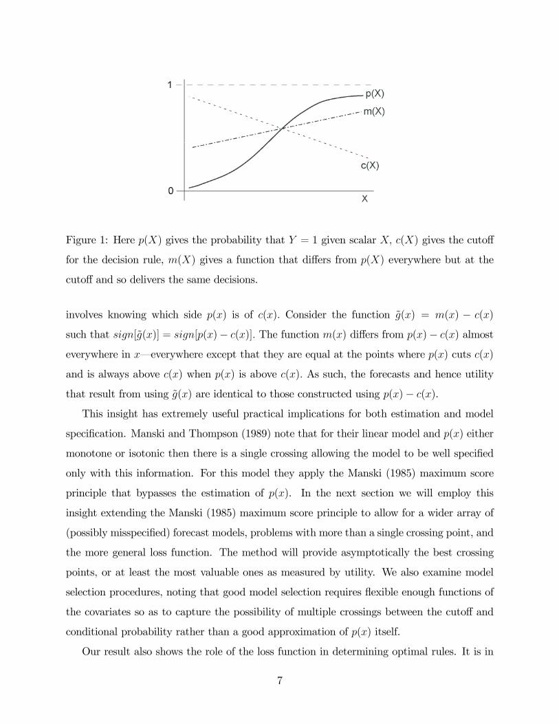
Figure 1: Here p(X) gives the probability that Y = 1 given scalar X, c(X) gives the cutoff
for the decision rule, m(X) gives a function that differs from p(X) everywhere but at the
cutoff and so delivers the same decisions.
involves knowing which side p(x) is of c(x). Consider the function g(x) = m(x) − c(x)
such that sign[g(x)] = sign[p(x)− c(x)]. The function m(x) differs from p(x)− c(x) almost
everywhere in x–everywhere except that they are equal at the points where p(x) cuts c(x)
and is always above c(x) when p(x) is above c(x). As such, the forecasts and hence utility
that result from using g(x) are identical to those constructed using p(x)− c(x).
This insight has extremely useful practical implications for both estimation and model
specification. Manski and Thompson (1989) note that for their linear model and p(x) either
monotone or isotonic then there is a single crossing allowing the model to be well specified
only with this information. For this model they apply the Manski (1985) maximum score
principle that bypasses the estimation of p(x). In the next section we will employ this
insight extending the Manski (1985) maximum score principle to allow for a wider array of
(possibly misspecified) forecast models, problems with more than a single crossing point, and
the more general loss function. The method will provide asymptotically the best crossing
points, or at least the most valuable ones as measured by utility. We also examine model
selection procedures, noting that good model selection requires flexible enough functions of
the covariates so as to capture the possibility of multiple crossings between the cutoff and
conditional probability rather than a good approximation of p(x) itself.
Our result also shows the role of the loss function in determining optimal rules. It is in
7

the roles of b(x) and c(x) in reweighting utility (discussed in context with estimation in the
next section) along with the insight that only crossing points need to be estimated well that
problems with the commonly applied two step approach to binary prediction of estimating
p(x) without reference to the loss function arise. Typically p(x) is estimated with reference
to an arbitrary loss function. For example probit and logit are estimated using maximum
likelihood (ML), an approach which is designed to provide the best global fit for the model
of p(x) to the data independent of both where it crosses c(x) and the relative importance of
various regions in X of having the correct forecast. Other methods such as neural networks
use quadratic loss, which suffers from the same problems as ML. We show in Section 4 that
these methods can be very poor predictors, even when they are close to being correctly
specified models.
3 Estimating Binary Prediction Models
3.1 The Maximum Utility (MU) Estimator
The optimal forecast/allocation method chooses a function g∗(·) that solves (4). For a
solution to this optimization problem, the forecaster must search over a function space.
More reasonably in practical situations the set of possible functions will be restricted and a
constrained optimization will be undertaken. Instead of considering all the possible functions
we restrict ourselves to a subset H of G and work with predictors of the form
P(H) = {sign[h(X)] : h ∈ H}.
We will parameterize the elements of H as h(x) = h(x, θ),where θ ∈ Θ ⊆ Rp, p ∈ N;
we will write HΘ for the parameterized class. Hence we have a parametric model for the
predictor function that is known up to the p−dimensional vector of unknown coefficients θ.
The optimal predictor is then obtained by solving
maxθ∈Θ
S(θ) ≡ maxθ∈Θ
EY,X{b(X)[Y + 1− 2c(X)]sign[h(X, θ)]}.
There is of course a cost to restricting the form of the predictors considered. It may well be
that the set of functions that maximize expected utility in the unconstrained problem, G∗,
8

are ‘locked out’ of HΘ, meaning that the set of optimal functions in the constrained problem,
H∗Θ, is also mutually exclusive of G
∗, Nevertheless if
∃θ∗ ∈ Θ such that sign[h(x, θ∗)] = sign[p(x)− c(x)] for all x ∈ support(X), (5)
then G∗∩H∗Θ is nonempty. In standard econometric language this means that for the model
to be optimal from a forecasting or classification standpoint, it does not have to be fully
correctly specified for p(x)− c(x); it is enough for it to be correctly specified for the sign of
p(x)− c(x). This gives clear insights in how to choose h(X, θ) (up to knowing θ) in practice.
Essentially all that is required to achieve the same prediction as knowing p(x) is that the
model be sufficiently flexible to capture all of the crossing points of p(x) and c(x).
The weaker requirement than correct specification of p(x) can be exploited practically
in simplifying model building. For example if we have a single predictor (k = 1) then a
polynomial in X of order d allows for d changes in the sign of the predictor as a function
of x. Knowing p(x) − c(x) only up to the number of sign changes is thus sufficient for
obtaining a correct specification of the forecasting model, even though p(x) itself is not known
well enough for correct specification. Knowing p(x) is monotonically increasing in x (and
knowledge of c(x) which comes from knowing the utility function) tells us exactly the number
of crossing points between p(x) and c(x) but does not tell us the correct parameterization of
p(x). For higher dimensional problems (k > 1) we can still use this insight, however concrete
implications become more difficult. Results for interesting cases are available however, as
shown in the following proposition.
Proposition 1 Let c ∈ R, β ∈ Rk, β 6= 0, and let Q : R → R be a function such that the
set Σ = {σ : Q(·) − c changes sign at σ} has at most a finite number of elements. Then
there exists a finite order polynomial h(x) and A ⊂ Rk with Lebesgue measure one such that
sign[h(x)] = sign[Q(x0β)− c] for all x ∈ A. If in addition Q is lower semicontinuous at each
σ ∈ Σ, then A = R.
Some examples can clarify the result. If c(X) is constant, Y ∗ = Q(X 0β)+U, Y = sign[Y ∗],
and U is independent of X with cdf FU(u), then p(X) = 1− FU [−Q(X 0β)] > c if and only
if Q(X 0β) > c, for c = − inf{u : FU(u) ≥ 1 − c} (see for example Horowitz (1998), Powell
9

(1994)). For a second example suppose that U is only (1 − c)−quantile independent of X,
i.e. inf{u : FU |X(u) ≥ 1 − c} is a constant −c that only depends on c but not the value of
X. Then it remains true that p(X) > c if and only if Q(X 0β) > c. This example provides a
generalization of the ’single crossing’ restriction of Manski and Thompson (1989).
If the set of maximizers of S(θ) is nonempty, then it will often contain more than one
element. We distinguish between two types of multiplicity. On the one hand,
P{sign[h(X, θ1)] = sign[h(X, θ2)]} = 1 (6)
may hold for distinct θ1, θ2 in argmaxS (θ) , i.e. the same optimal partition of the covariate
space under the model HΘ may be induced by more than one value of θ. Alternatively, it
might happen that the optimal partition itself is not unique so that θ1 and θ2 both maximize
S(θ), but (6) fails to hold.
Multiple maxima of the first type arise quite generally; an example is that the linear
model is only identified up to scale (Manski (1985), Horowitz (1992)). Another example is
provided by discrete X – in this case most values of θ will have an entire neighborhood of
points leading to the same decision rule. In contrast, multiple maxima of the second type are
non-generic. Their existence is predicated on rare coincidences between the decision maker’s
utility function, the parameterization HΘ, and the joint distribution of Y and X.
While lack of identification is an issue when θ is a structural parameter endowed with
economic content, multiple maxima of S(θ) are of little concern in the present forecasting or
classification context. First, the modelHΘ is not intended to play a role or have any meaning
beyond approximating the optimal decision rule sign[p(x)− c(x)]. Second, taking the utility
maximization problem literally means that the decision maker will be indifferent between two
parameter vectors that result in the same level of utility. For these reasons our analysis will
focus on the properties of the optimand function instead of the usual econometric focus on
the optimizers, which could be considered as nuisance parameters of the forecasting problem.
To estimate a member of H∗Θ based on a finite set of data, we suggest the sample analog
of the expected utility maximization problem that results in the set of models HΘ. Given a
10

sample of observations {(Yi, X 0i)}ni=1, choose θ to solve
maxθ∈Θ
Sn(θ) ≡ maxθ∈Θ
n−1nXi=1
b(Xi)[Yi + 1− 2c(Xi)]sign[h(Xi, θ)].
For b(Xi) constant, c(Xi) = 0.5 and h(Xi, θ) = X 0iθ this is Manski (1985)’s maximum
score estimator. When the estimation procedure searches over candidate functions, the goal
is to match the sign of Yi with the sign of h(Xi, θ). By determining the value of each match
through the weights b(Xi)[Yi + 1 − 2c(Xi)], the utility function plays a direct role in the
estimation of the parameters. As earlier, c(Xi) determines the relative value of correct
prediction when Yi = 1 relative to correct prediction when Yi = −1, whereas b(Xi) controls
the value of correctly predicting Yi for that individual regardless of Yi. This term is only
important if the model is not correctly specified, i.e. the modelHΘ cannot possibly reproduce
the theoretically optimal predictor for all values of X. In this case the trade-offs in finding
the expected utility maximizing fit conditional on model specification will be guided partly
by the function b(.). If the model were correctly specified one could replace b(.) by any other
bounded positive function (which may not correspond to the utility function at all) and the
fitted model will still reproduce sign[p(x) − c(x)] asymptotically. (Small sample fit would
be affected).
Given the observed data, Sn(θ) can take on at most 2n different values as a function of θ,
regardless of the specification of h(x, θ). For each θ, Sn(θ) is a sum of n terms, only the sign
of each term depends on θ. Thus even if each sign could be set independently of the others,
the sum could take on 2n distinct values. As the range of Sn(θ) is finite over Θ, a maximum
must always exist.
It is clear that maximization of Sn(θ) in practice cannot be undertaken by hill climbing
methods. The Monte Carlo studies presented in Section 4 demonstrate that the simulated
annealing algorithm (see Corona et. al. (1987) and Goffe et. al. (1984)) is robust enough
to handle the nonstandard feature of the objective function under consideration here.
11

3.2 Asymptotic Properties of the MU estimator
As noted above, instead of studying the convergence of θn, we will focus on the conver-
gence properties of the maximized value of the sample objective. We first establish uniform
convergence of Sn(θ) to S(θ), consistency follows directly. Under additional assumptions,
maxθ Sn(θ) converges at the usual rate and is asymptotically normal.
Using only the assumption that the data are i.i.d., Manski (1985, Lemma 4) establishes
a.s. uniform convergence of Sn(θ) to S(θ) in the special case when h(x, θ) = x0θ, and the
utility function does not depend on x. The proof cites a Glivenko-Cantelli type result by Rao
(1962) whose applicability depends critically on the geometry of the linear model. As we
allow for general functional forms and serially dependent data, we need to extend Manski’s
result. We impose some (joint) restrictions on the model HΘ and the distribution of X.
Condition 2 (i) Θ ⊂ Rp is compact; (ii) The function (x, θ) 7→ h(x, θ) is jointly Borel
measurable and Lipshitz-continuous over Θ, i.e. there exist constants M2 > 0 and λ > 0
such that |h(x, θ)− h(x, θ0)| ≤M2 kθ − θ0kλ for all θ, θ0 ∈ Θ and x ∈ support( X).
As θ varies over Θ, h(X, θ) might act as a continuous variable for some values of θ and
as a discrete one for others. In the latter case it is possible that h(X, θ) = 0 happens with
positive probability, creating a discontinuity in the function S(θ). The following condition
ensures these discontinuities do not interfere with uniform convergence.
Condition 3 There exists a subset Θ0 of the parameter space such that (i) supθ∈Θ0 P [−δ ≤
h(X , θ) ≤ δ] ≤ M3δr for some constants M3 > 0, r > 0 and ∀δ > 0 sufficiently small; (ii)
if θ /∈ Θ0, then the function x 7→ h(x, θ) is either constant, or depends at most on discrete,
finitely supported components of X.
Restricted to Θ0, S(θ) is a (uniformly) continuous function of θ, while restricted to
Θ/Θ0 it is a step function (Lemma 2 in appendix). It is possible for Θ0 to be equal to
the entire parameter space or be empty. Condition 3(i) is somewhat stronger than having
P [h(X, θ)] = 0] = 0 for all θ ∈ Θ0. It is satisfied if for each θ in Θ0 the distribution of the
random variable h(X, θ) is absolutely continuous (possibly conditional on some components
12

of X), and the associated densities are bounded in a neighborhood of zero uniformly over Θ0.
For example, let h(X, θ) = θ1 + θ2X, θ ∈ [−1, 1]× [−1, 1], where X is has bounded density
f(x) with xf(x) also bounded. Then h(X, θ) has the density z 7→ 1θ2f³z−θ1θ2
´for θ2 6= 0. This
density is bounded for, say, z ∈ (−0.1, 0.1) uniformly over θ ∈ Θ0 = {12} × ([−1, 1]\{0}),
and for θ /∈ Θ0, h(X, θ) is constant as a function of X. In contrast, Manski (1985) and
Horowitz (1992) normalize the parameter space (and restrict the distribution of X) to ensure
P (X 0θ = 0) = 0 for all θ ∈ Θ, essentially requiring Θ = Θ0. In a pure forecasting context
such normalizations would be hard to motivate – Condition 3 makes them unnecessary.
Finally, we restrict the sampling process, while allowing for serially dependent observa-
tions recorded over time.
Condition 4 For p, λ and r as in Conditions 2 and 3, letW denote the smallest even integer
greater than 4p/rλ. Then {(Yi,X 0i)}ni=1 is a strictly stationary, mixing sequence of observa-
tions from (Y,X 0), defined on a complete probability space, with strong mixing coefficients
α(d) = O(d−A), where A > (W − 1)(1 +W )/2.
The following result extends Manski (1985, Lemma 4).
Proposition 2 Given Conditions 1 through 4, then (a) supθ∈Θ |Sn(θ)− S(θ)|→ 0 w.p.1 as
n → ∞, (b) maxθ∈Θ Sn(θ) → supθ∈Θ S(θ) w.p.1 as n → ∞. Further if θn is a measurable
selection from argmaxθ∈Θ Sn(θ), then (c) S(θn)→ supθ∈Θ S(θ) w.p.1 as n→∞.
It is part (c) of Proposition 2 that provides the basic justification of the proposed es-
timation method. It states that the expected utility derived from classifications using θn
approaches the upper bound of utility levels achievable under the parameterization HΘ, re-
gardless of whether this parameterization satisfies (5). The result relies on the function we
are maximizing and the target function getting close asymptotically, but does not rely on
the maximizer θn getting close to a ’true’ set of optimal coefficients. In fact, the conditions
of Proposition 2 are not generally sufficient to guarantee that there exists an optimal value
of θ that attains the supremum. In contrast to the above, the existence of a ’nice’ set of
maximizers of S(θ) is assumed to show asymptotic normality of maxθ Sn(θ). No analogous
result is given in the maximum score literature.
13
Condition 5 Let Θ∗ = argmaxθ∈Θ S(θ) and Θ∗ε = {θ ∈ Θ : d(θ,Θ∗) ≤ ε}. (i) Θ∗ 6= ∅ and
Θ∗ε ⊂ Θ0 for some ε > 0. (ii) supθ∈Θ\Θ∗ε S(θ) < maxθ∈Θ S(θ) for all ε > 0. (iii) θ, θ ∈ Θ∗
implies (6). (iv) P [sign(h(X, θ∗)) = Y ] 6= 1 for θ∗ ∈ Θ∗.
Whilst these are fairly high level conditions, they are not unreasonable. Given that
S(θ) is continuous (and bounded) over Θ0, and is a step function otherwise, the existence
of a maximum is not a big leap of faith – the only part of the parameter space that can
potentially cause problems, when Θ 6= Θ0 and Θ0 6= ∅, is the boundary of Θ0. In addition,
Condition 5(i) requires that h(X, θ) acts as an absolutely continuous random variable for
values of θ in the neighborhood of Θ∗. Barring unusual parameterizations, this will be the
case if, conditional on the rest of X, some component of X is absolutely continuous and
provides some useful information about Y. Neither this condition nor Condition 3 imposes
full support or smoothness on the conditional density (or a related density), unlike Manski
(1985), Horowitz (1992) and Kim and Pollard (1990). Condition 5(ii) states that the function
S(θ) has a ’clean’ maximum, i.e. one cannot get arbitrarily close to the optimum in a part of
the parameter space that is disconnected fromΘ∗. Condition 5(iii) rules out non-generic type
of multiple maxima discussed in Section 3.1, Condition 5(iv) disallows perfect predictors.
We now have a set of conditions sufficiently strong to establish the asymptotic distribution
of maxθ Sn(θ). Define the asymptotic variance function as
V (θ) = var[s(Y1,X1, θ)] + 2∞X
m=2
cov[s(Y1,X1, θ), s(Ym,Xm, θ)],
where s(y, x, θ) = b(x)[y+1−2c(x)]sign[h(x, θ)]. For i.i.d. data the covariance terms vanish
and the formula reduces to
V (θ) = E©b(X)2[Y + 1− 2c(X)]2
ª− [S(θ)]2.
Hence, in this case V (θ) depends on θ only through S(θ), and is therefore constant over Θ∗.
For serially dependent data the covariance terms can be written as
Enb(X1)[Y1 + 1− 2c(X1)]sign[h(X1, θ)]b(Xm)[Ym + 1− 2c(Xm)]sign[h(Xm, θ)]
o− [S(θ)]2.
Under Condition 5(iii), sign[h(X, θ∗1)] = sign[h(X, θ∗2)] w.p. 1 for any two maximizers θ∗1, θ
∗2 ∈
Θ∗. Therefore, given this additional assumption, V (θ∗) does not vary with θ∗ ∈ Θ∗ even
14

when the data points are serially dependent. Let S∗ and V ∗ denote the values of S(.) and
V (.) over Θ∗. Then:
Proposition 3 Given Conditions 1-5, (a) n1/2[maxθ∈Θ Sn(θ)− S∗] −→d N(0, V ∗), V ∗ > 0,
and (b) n1/2[S(θn)− S∗] = op(1).
This result establishes the rate of convergence of the decision maker’s utility, both in
sample and out of sample. For in sample evaluation (evaluation of maxθ∈Θ Sn(θ)), the con-
vergence rate is exact. When a sample estimate is used for out of sample evaluation without
re-estimation of the parameter (evaluation of S(θn) where both the estimation sample and
evaluation sample become large), the convergence rate is a lower bound. With an estimate
of V ∗, part (a) also allows construction of a confidence interval for S∗, the maximum utility
achievable under the model specification. This result can also be used to test that utility
achieves a certain level.
In the case where the data is i.i.d. Proposition 3 can be employed to test between speci-
fications4. Suppose that we have a model h1(x, θ1) and wish to compare with another model
h2(x, θ2), where h2(x, θ2) nests h1(x, θ1). For example, h1(x, θ1) could be a linear specifica-
tion, while h2(x, θ2) could also include quadratic terms. We can test the null hypothesis that
S1(θ∗1) = S2(θ
∗2) against the alternative that S1(θ
∗1) < S2(θ
∗2). Construct an i.i.d. sequence
of Bernoulli(λ) random variables {Zi}ni=1, independent of the data, and compute
S1n = maxθ1∈Θ1
S1n(θ1) ≡ maxθ1∈Θ1
n−1nXi=1
b(Xi)[Yi + 1− 2c(Xi)]sign[h1(Xi, θ1)]
and
Sλ2n = max
θ2∈Θ2Sλ2n(θ2) ≡ max
θ2∈Θ2n−1
nXi=1
Zib(Xi)[Yi + 1− 2c(Xi)]sign[h2(Xi, θ2)].
Hence, one specification is estimated on the full sample, while the other on a random sub-
sample picked out by the Bernoulli variables. It is straightforward to generalize the proof of
Proposition 3 to show that the asymptotic distribution of S1n and Sλ2n is jointly normal and
4There are a large number of methods for model selection for classification schemes, although none have
been shown to extend to the general methods of this paper.
15

derive an explicit expression for the variance-covariance matrix (see the Appendix). Under
the the null hypothesis it follows in particular that
n1/2³λS1n − Sλ
2n
´−→d N(0, σ2λ),
where σ2λ = λ(1−λ)E[b(X)2(Y +1−2c(X))2]. Using the sample analog principle, a consistent
estimator for σ2λ is easy to construct.
4 Finite Sample Properties: Monte Carlo Results
We present simulation evidence to give both empirical content to the theoretical results in
Section 2 that suggest potential issues in estimating p(x) to construct forecasts and also to
demonstrate the performance of the methods suggested in Section 3. To do this we present
two data generating processes (DGP’s) and two sets of utility functions for each DGP. As
utility has no natural units, we will compare the ratio of utility for any model to the utility
that would be gained if p(x) were known (the PK model, where infeasible forecasts are
constructed from the known p(x)−c(x)). We will refer to this ratio as relative utility (RU)5.
For each DGP and utility function we present both in and out of sample results for the
prediction method. For the same reasons that R2 is always nondecreasing in the number
of terms in a linear regression, by the properties of maximization the in sample results will
always favor larger models. By the same token, they will often outperform the PK model
for the sample. The in sample results are none-the-less interesting as a gauge of the extent
of the ’overfitting’ of the methods to the data. The larger the gain over the PK model the
greater the ability of the model and method to find incidental matches in the data that do
not reflect features of the DGP. The out of sample results are of course directly interesting
as they examine how well the estimation fits the model on a new set of data.
The first model for the Monte Carlo study is given by p(X) = Λ(−0.5X + 0.2X3) where
Λ(.) is the logit function. The distribution for X is U(−2.5, 2.5). Figure 2 shows p(x) over
this support. We draw 75 in sample observations (for estimation) and 5000 out of sample
5Since a constant added to S(·) will change the ratio, we normalize as follows. Set u−1,−1(x) = u−1,1(x) =
0, which amounts to representing expected utility as 0.25S + 0.25E [b(X)(Y + 1− 2c(X)].
16

Figure 2: The solid line shows p(x). Dashed lines are c(x) for P1 (flat line at 0.5) and P2
(upward sloped line). The dot-dash line shows an estimated linear probit model fit of p(x).
The histogram at the bottom of the figure is for a draw of the X variable.
observations (for evaluation). The number of Monte Carlo replications is 500. This model is
chosen so that it is sufficiently flexible to enable multiple crossings (so that the categorization
is not simply a crossing point) but the cubic logit model is correctly specified. The model
p(X) is sufficiently close to the single threshold model Λ(−0.5X) that 5% LagrangeMultiplier
(LM) tests of this null model reject for the model that includes bothX2 andX3 with roughly
33% power only. We choose a local misspecification because it is precisely these types of
misspecifications that are unknown to the researcher. In terms of utility we examine two
sets of preferences, first setting c(x) = 0.5 (P1) and in the second c(x) = 0.5 + 0.025x (P2),
shown in Figure 1 by the dashed lines. We set b(x) to be constant, the value of this constant
has no effect on the relative utility. For both utility functions there are three crossing points.
Results are presented in Table 1.
The cubic ML model here is correctly specified for p(x) – it follows directly that the
difference between this model and PK is due only to estimation error of the model para-
meters; asymptotically it will obtain the highest possible utility. It is no surprise then that
17

Table 1: Model 1 - Possibly Correctly Specified MLE
ML MU
Lin Cubic Mix 1 Lin Cubic Mix 1 Mix 2
In/Out In/Out In/Out In/Out In/Out In/Out In/Out
RU (P1) 86.2/37.0 139.4/73.1 120.2/52.7 146.1/50.3 226.0/67.1 179.4/57.3 201.2/61.5
RU (P2) 77.2/11.6 140.9/67.1 115.1/36.0 139.1/31.9 230.9/61.3 177.0/45.2 206.8/53.7
Correct(P2) 58/53 63/57 61/54 63/54 71/56 67/55 69/56
Note: The first two rows denote relative utility (RU), as defined in the first paragraph of Section 4
and expressed as a percentage, for P1 and P2. The last row is the percentage of correctly classified
observations for P2. "In" refers to the in sample result, "Out" to the out of sample result.
this method performs best. As there are three crossing points for both preferences, the
cubic MU method is also correctly specified. Hence differences between this model and PK
also represent estimation error. The correctly specified ML method performs better than
the MU method, reflecting the gain of parametric methods over semiparametric methods
when the parametric specification is correct. This effect however is small. Comparing the
(misspecified) linear models MU performs far better than ML. A best linear choice would
be the approximation that maximizes utility. However, as noted at the end of Section 2,
the ML method instead provides a best fit of p(x) over all of the range of X whereas MU is
designed to focus estimation on getting the points and signs correct around the points where
p(x) cuts c(x).With a linear specification this means choosing the best single crossing point
of c(x). Gains from doing so in a misspecified model can be very large, as we see in the
Monte Carlo results. These differences are not well reflected in the percentage of correctly
classified observations. For example under P2 the linear MU model correctly classifies 54%
of the observations out of sample, just one percentage point less than the cubic model, but
the difference in the relative utilities is large. We can also see that the size of the effect
depends on the utility function; in Table 1 the gain is larger for the second set of preferences
despite the differences between the preference configurations being small. If we believe that
models are approximations, using a method that is robust such as MU over a method that
is not such as ML seems appropriate.
18

In sample overfitting can be examined by comparing the in sample and out of sample
results. Both ML and MU have a strong tendency to overfit in sample, however the problem
seems more severe for the MU method. This creates challenges for model selection. We
examine a standard hypothesis test approach to selecting between the two models where for
each draw of the pseudo variables we test the null of the linear model against the cubic using
a size 5% LM test. We then apply both estimators to the model chosen (denoted ML Mix 1
and MU Mix 1, respectively). For the MU method we also use a size 5% test with λ = 0.75
based on the asymptotic results at the end of Section 3 (denoted MU Mix 2). The power of
the LM test to reject the linear model is 33% as noted above. This is enough to partially
offset the very poor performance of the ML method in this misspecified model for both sets
of preferences. However, relative out of sample utility for ML Mix 1 is still smaller than for
MUMix 1 (52.7% vs. 57.3% for P1 and 36% vs. 45.2% for P2). This is because the extent to
which ML outperforms MU in the correctly specified model is overpowered by the nontrivial
chance of misspecification and the extent to which MU outperforms ML in this case. The
mixture based on the asymptotic theory of this paper is better again–-in the out of sample
results this method gains 61.5% of available utility for P1 and 53.7% for P2. This additional
improvement over the performance of MU Mix 1 is due to the fact that the MU based test
rejects the linear model with almost 66% probability (the test has power precisely against
those types of misspecifications that matter for optimal classification).
The second DGP for the Monte Carlo study is a special case of the models in Proposition
1. The conditional probability is given by p(X) = Λ (Q(1.5X1 + 1.5X2)) where
Q(σ) =1.5− 0.1σ
exp(0.25σ + 0.1σ2 − 0.4σ3) .
The distribution for (X1, X2) is uniform on [−3.5, 3.5]× [−3.5, 3.5]. Figure 3 shows Λ(Q(σ))
over part of the range of 1.5X1+1.5X2 (solid line). This model corresponds to a heteroskedas-
tic linear index model Y ∗ = 1.5 − 0.1σ + exp [0.25σ + 0.1σ2 − 0.4σ3] with Y = sign(Y ∗).
Two variations on the utility model are examined to highlight the effect of the utility function
on the performance of each of the methods. In the first specification (P3) we set c(x) = 0.75
and b(x) = 20. The second (P4) varies b(x) by setting it to 60 for −1.5 < x1 + x2 < 1.5 and
keeping it at 20 otherwise. The dashed line gives c(x) for both utility functions, showing
19

Figure 3: The solid line shows Q(σ), the dashed line is c(x) for both P3 and P4.
again three crossing points. The estimation sample has 500 observations and the out of
sample evaluation 5000 observations.
Results are given in Table 2. Even though the specification of p(X) is complicated, there
are only three crossing points in terms of the index σ for both preferences. As Proposition
1 indicates, a cubic model in X, including all cross products, is correctly specified for the
MU method. This is in contrast with ML estimation where any logit model with a finite
dimensional polynomial in X will be misspecified for p(X). Examining the out of sample
results, all of the MU models outperform all of the ML models, even the most parsimonious
MU model performs better than the best ML model. This reflects the difficulties mentioned
above regarding the misspecified MLE and the ability of the MU method to still choose
crossing points when the model is misspecified for p(x) as a whole. The cubic MU model,
which is correctly specified in the sense of capturing crossing points, is the best performer
of the individual models in terms of both relative utility and also in correctly classifying the
observations.
For P4 we vary the utility function to make observations towards the center of the
distribution more important for utility. With this reweighting, both methods do less well in
20

Table 2: Model 2 - Incorrectly Specified MLE
ML MU
Lin Cubic Mix 1 Lin Cubic Mix 1 Mix 2
In/Out In/Out In/Out In/Out In/Out In/Out In/Out
RU (P3) 64.8/59.8 76.5/60.1 72.5/60.1 94.2/70.9 134.7/81.4 111.2/74.6 128.0/79.6
RU (P4) 41.1/30.2 61.0/34.2 54.8/33.0 94.8/57.4 158.5/71.9 122.0/63.1 147.6/68.5
Note: The first two rows denote relative utility (RU), as defined in the first paragraph of Section
4 and expressed as a percentage, for P3 and P4. "In" refers to the in sample result, "Out" to the
out of sample result.
terms of relative utility, however the loss for ML is much larger than for MU (the former
dropping by about one half compared to the first utility specification). Comparing the best
ML model with the best MU model for P3 (out-of-sample) we see that the ML method picks
up 60% of the possible utility whereas MU picks up over to 80% of this available utility. For
P4 the relative difference is larger, with ML picking up 34% and MU 72% of the available
utility. This demonstrates the importance of the utility function in the semiparametric
estimation procedure, and the impact it can have on the parametric methods’ performance.
The mixture models here examine three specifications – the linear and cubic models
(each individually reported in the table) as well as a quadratic specification (not individu-
ally reported). The selection procedure consists of testing down from the cubic specification
towards the linear using the two tests described above; the three mixtures are then con-
structed in a similar way. As the mixture model with ML did relatively poorly when one
of the ML models was correctly specified, it is no surprise that the same is true when all
the ML models are not correctly specified. The gap between ML Mix 1 and MU Mix1 is
considerable for P3 and even larger for P4. The method suggested in this paper (MU Mix
2) claims nearly all of the utility gained by the best single (cubic) MU model, and performs
better than MU Mix 1.
Finally, rather than employing the semiparametric approach of the MU method, under
lack of knowledge of the model for the conditional probability we might consider nonpara-
metric estimation. In Table 3 we compare the two methods above to results obtained from
21

Table 3: ML vs. MU vs. nonparametric methods
DGP DGP 1 DGP 2
P1 P2 P3 P4
Method In/Out In/Out In/Out In/Out
Nonparametric 155.3/49.2 153.2/35.4 112.9/74.8 121.1/58.8
ML(cubic) 139.4/73.1 140.9/67.1 76.5/60.1 61.0/34.2
MU(cubic) 226.0/67.1 230.9/61.3 134.7/81.4 158.5/71.9
Notes: The entries are relative utility (RU), as defined in the first paragraph of Section 4 and
expressed as a percentage, for each utility function. "In" refers to the in sample result, "Out" to
the out of sample result
using a nonparametric (kernel) estimator for p(X). Specifically, a nonparametric regression
of Y on X using the Nadaraya Watson kernel with the bandwidth chosen using least squares
cross validation over the estimated sample. The results are summarized for both of the
DGP’s, where we have also included the best performer of the ML and MU models.
In general a consistent nonparametric estimator for p(X) should attain the best utility
asymptotically, however in practice we expect that its lack of focus on the crossing points
will mean that in real samples it will have similar problems as other non loss based estima-
tors. Of course we also expect that in sample problems of overfitting will be important as
well. When the correct parametric specification is available, we expect that a nonparametric
method would suffer from not utilizing this information. This is indeed borne out in Table
3. For the first DGP, the correctly specified ML(cubic) method has the best out of sample
performance in terms of RU for both P1 and P2. With as few as 75 observations for estima-
tion, the nonparametric method (which does not utilize the knowledge implicit in the cubic
specification), performs considerably worse than ML or MU, capturing less than half of the
available utility out of sample. For the second DGP, MU still outperforms the nonparamet-
ric method despite the fact that there are 500 observations in the estimation sample (X is
however two dimensional). As discussed in Section 2, requiring only the knowledge of the
number of turning points and the use of the utility function in the estimation of the crossing
points results in a very useful method in misspecified models.
22

5 Conclusion
When making binary predictions or classifications with exogenous predictors, this paper
provides an estimation method grounded in a general family of utility functions that has
the property that, at least asymptotically, the method delivers the highest possible utility
given the functional form of the model. Since the estimation procedure is geared towards
fitting the optimal decision rule directly, this result does not rely on knowing the correct
specification of p(X). This turns out to be extremely useful when models are misspecified,
a situation that is likely in practice and one where parametric models can perform very
poorly. The estimation problem extends the Manski maximum score model, where the
extensions are to different weighting functions and also generalizing the model beyond linear
index functions. These extensions are possible since the focus is on the objective function
rather than the model parameters. We present asymptotic theory showing consistency and
asymptotic normality of the score function. The asymptotic results can also be used to test
which of two parameterizations is closer to the maximal utility attainable given the models.
The Monte Carlo results support one of the main points of the paper – estimating
a decision rule based on p(X) is an exercise that requires different tools than estimating
p(X) itself. The typical alternative approach of employing a probit or logit model can
result in very poor performance in misspecified models. Employing the utility function in
the classification/forecast problem is thus shown to be important for attaining the maximal
utility.
6 Appendix: Proofs
Proof (Proposition 1) Let N = #Σ < ∞. If N = 0, set h(x) to a constant and A = R. If
N > 0, let σ1 < ... < σN be elements of Σ. Define Ki = 2 if σi is a strict local minimum of Q
and Ki = 1 otherwise. Setting L(σ) equal to one of the polynomials ±ΠNi=1(σ − σi)Ki produces
sign[L(σ)] = sign[Q(σ) − c] for all σ except possibly at those σi at which Q is discontinuous (in
this case Q(σi) − c > 0 is possible whereas L(σi) = 0). Let Σ0 ⊂ Σ denote the set of such σi. Set
h(x) = L(x0β) and A = {x : x0β = σi, for some σi ∈ Σ0}c. Since L(σ) is a polynomial of finite
23

order, so is x 7→ h(x), and the set A has Lebesgue measure 1. Finally, if Q is lower semicontinuous
at σi, then Q(σi) ≤ c so that sign[L(σi)] = sign[0] = −1 = sign[Q(σi)− c] ∀σi.
Lemma 1 Under Conditions 1,2 and 3, there exists constants K > 0 and q > 0 such that, for
all δ > 0 sufficiently small, supθ0∈Θ0 Ensupθ∈B(θ0,δ)∩Θ0 |s(Y,X, θ)− s(Y,X, θ0)|2
o≤ Kδq, where
B(θ0, δ) is the Euclidean open ball with radius δ centered on θ0.
Proof Fix θ0 ∈ Θ0 and any δ > 0. By Condition 1, |b(x)[y + 1− 2c(x)]| ≤ 4M1. We can write
E supθ∈B(θ0,δ)∩Θ0
|s(Y,X, θ)− s(Y, x, θ0)|2 ≤ 2(4M1)2E sup
θ∈B(θ0,δ)∩Θ0|sign[h(X, θ)]− sign[h(X, θ0)]|.
(7)
By Condition 2 part (ii), there exist constants λ > 0 and M2 > 0 such that, with prob. 1,
h(X, θ) ∈ [h(X, θ0)−M2δλ, h(X, θ0) +M2δ
λ] ∀θ ∈ B(θ0, δ) ∩Θ0.
Thus for θ ∈ B(θ0, δ) ∩ Θ0, sign[h(X, θ)] 6= sign[h(X, θ0)] implies that the interval above must
contain zero, i.e. h(X, θ0) must lie in [−M2δλ,M2δ
λ]. More formally,
|sign[h(X, θ)]− sign[h(X, θ0)]| ≤ 2× 1n−M2δ
λ ≤ h(X, θ0) ≤M2δλo∀θ ∈ B(θ0, δ) ∩Θ0.
Taking the sup of the lhs over θ, taking expectations of both sides, combining with (7), and then
taking the sup over θ0 yields
supθ0∈Θ0
E supθ∈B(θ0,δ)∩Θ0
|s(Y,X, θ)− s(Y, x, θ0)|2 ≤ 4(4M1)2 supθ0∈Θ0
P [−M2δλ ≤ h(X, θ0) ≤M2δ
λ]. (8)
By Condition 3(i), the rhs of (8) is less than or equal to 64M21M3M
r2 δ
rλ for some M3, r > 0 and
all δ > 0 sufficiently small, so K = 64M21M
r2M3 and q = rλ.
Lemma 2 Under Conditions 1, 2, and 3, the function S(θ) is (a) uniformly continuous over Θ0,
and (b) has a finite number of possible values over Θ1 = Θ\Θ0.
Proof Part (a): Using Lemma 1, as δ ↓ 0 then sup©|S(θ)− S(θ0)| : θ, θ0 ∈ Θ0, ||θ − θ0|| ≤ δ
ªgoes
to zero. Part (b): By Condition 3(ii), for each θ ∈ Θ1, h(X, θ) = h1(Xd, θ), whereXd is a sub-vector
of X, and Xd has finite support. For θ ∈ Θ1,
S(θ) =X
xd∈sup p(Xd)
Enb(X)[Y + 1− 2c(X)]1(Xd = xd)
osign[h1(x
d, θ)].
By the same argument employed in the text to show Sn(θ) has finite range over Θ, this decompo-
sition shows that S(θ) has at most 2#sup p(xd) possible values over Θ1.
24

Lemma 3 Under Conditions 1-4 supθ∈Θ0 |Sn(θ)− S(θ)|→a.s. 0.
Proof We apply a modified version of Andrews (1987) to the sequence of random variables
{s(Yi,Xi, θ)} to obtain a uniform LLN. The modification is explained in footnote 1 of Andrews
(1992). By Condition 2(i), Θ0 is (totally) bounded. By Condition 4 and Lemma 1, Assumption
A3 of Andrews (1987) holds uniformly over Θ0; see comment 3 following Theorem 1 in Andrews
(1987) and footnote 1 in Andrews (1992). By Condition 4, Assumption B1 in Andrews (1987) is
satisfied. As in Lemma 1, supθ∈Θ0 |s(Yi,Xi, θ)| ≤ 4M1, so Assumption B2 of Andrews (1987) is
satisfied. (The measurability conditions can be argued from Appendix C of Pollard 1984). Lemma
3 then follows from Corollary 1 of Andrews (1987) and footnote 1 of Andrews (1992).
Lemma 4 Under Conditions 1-4, supθ∈Θ1 |Sn(θ)− S(θ)|→a.s. 0.
Proof Let w(y, x) = b(x)[y+1− 2c(x)]. For each θ ∈ Θ1, we use the decomposition of S(θ) in the
proof of Lemma 2 and the analogous decomposition of Sn(θ) to write
|Sn(θ)− S(θ)| =
¯¯ Xxd∈sup p(Xd)
½n−1
nPi=1
w(Yi,Xi)1{Xdi = xd}−E[w(Y,X)1{Xd = xd}]
¾sign[h1(x
d, θ)]
¯¯
≤X
xd∈sup p(Xd)
¯n−1
nPi=1
w(Yi,Xi)1{Xdi = xd}−E[w(Y,X)1{Xd = xd}]
¯,
By the SLLN for stationary ergodic sequences (e.g. Thm 3.34 of White 2000), for any fixed value of
xd the corresponding term inP
xd goes to zero wp.1 as n→∞. As this sum is finite, the sum also
goes to zero. Finally, as this upper bound does not depend on θ, supθ∈Θ1 |Sn(θ)−S(θ)|→a.s. 0.
Proof (Proposition 2). Part(a): Immediate from Lemmas 3 and 4. Part (b): For any two
real-valued functions f and g defined on a set D, the inequality |supx∈D f(x)− supx∈D g(x)| ≤
supx∈D |f(x)− g(x)| holds. Apply to Sn(θ), S(θ) and Θ. Part (c): Using part (b)¯supθ∈Θ
S(θ)− S(θn)
¯≤¯supθ∈Θ
S(θ)− Sn(θn)
¯+¯Sn(θn)− S(θn)
¯≤ 2 sup
θ∈Θ|Sn(θ)− S(θ)| ,
which goes to zero by (a).
Lemma 5 Let θn be a measurable selection from argmax .Sn(θ). Under Conditions 1-5, d(θn,Θ∗)→a.s.
0, where d(., .) is the Euclidean metric.
25

Proof Suppose not. Then, with positive probability, there exists > 0 such that d(θnj ,Θ∗) >
along a subsequence θnj . By Condition 5(ii), supj S(θnj ) < S∗. However, Proposition 2(c) implies
S(θnj )→ S∗ w.p.1 as j →∞, which is a contradiction.
Lemma 6 Under Conditions 1-5, ρ(θn, θ∗) →a.s. 0 ∀θ∗ ∈ Θ∗ where ρ is the semimetric on Θ
defined by ρ(θ1, θ2) =©E£|s(Y,X, θ1)− s(Y,X, θ2)|2
¤ª1/2.
Proof Condition 5(i) and Lemma 2 imply Θ∗ ⊂ Θ0 is closed. Therefore, ∃θ∗n ∈ Θ∗ such that
d(θn,Θ∗) = d(θn, θ
∗n) for each n. For these θ∗n, for any fixed θ∗ ∈ Θ∗, ρ(θn, θ∗) ≤ ρ(θn, θ
∗n) +
ρ(θ∗n, θ∗) = ρ(θn, θ
∗n) since the ρ−distance between any two elements of Θ∗ is zero under Condition
5(iii). Let rn = d(θn, θ∗n) + 1/n. By Lemma 5, rn →a.s. 0, so using Lemma 1, one can find n large
enough so that
ρ(θn, θ∗n) ≤
(supθ0∈Θ
E
"sup
θ∈B(θ∗n,rn)|s(Y,X, θ)− s(Y,X, θ0)|2
#)1/2≤ (Krqn)
1/2
for some K, q > 0. Letting n go to infinity completes the proof.
Lemma 7 Under Conditions 1-5, the function Jn(θ) = n1/2[Sn(θ)−S(θ)] is stochastically equicon-
tinuous w.r.t. the semimetric ρ.
Proof We verify the Assumptions of Theorem 2.2. of Andrews and Pollard (1994), where {s(·, ·, θ) :
θ ∈ Θ} plays the role of F and {(Yi,X 0i)} plays the role of {ξi}. From Condition 4 the mixing
coefficients satisfy the summability condition in Thm 2.2 of Andrews and Pollard (1994) with
γ = 2. From Lemma 1 and the discussion preceding Theorem 2.2 the bracketing numbers of the
class {s(·, ·, θ) : θ ∈ Θ} are O(x−β) with β = 2p/rλ. By the discussion following the same theorem,
Condition 4 implies that the integral condition on the bracketing numbers holds with γ = 2.
Proof (Proposition 3). Write n1/2 [maxθ∈Θ Sn(θ)− S∗] = n1/2 [Sn(θ∗)− S(θ∗)]+n1/2
hSn(θn)− Sn(θ
∗)i,
where θn is a measurable selection from argmaxSn(θ) and θ∗ is a fixed element of Θ∗. A CLT that
applies to the first term of this decomposition under the stated conditions is given by Ibrag-
imov and Linnik (1971). V ∗ > 0 under Condition 5(iv). Further, Lemmas 6 and 7 imply
Jn(θn)−Jn(θ∗) = op(1) or, after rearrangement, n1/2[Sn(θn)−Sn(θ∗)]+n1/2[S(θ∗)−S(θn)] = op(1).
Since θn is a maximizer of Sn and θ∗ is a maximizer of S, both terms of the sum are nonnegative,
implying that n1/2[Sn(θn) − Sn(θ∗)] must itself be op(1).Since θnis a maximizer of Sn and θ∗is a
26

maximizer of S, both terms of the sum are nonnegative, implying that n1/2[Sn(θn) − Sn(θ∗)] and
n1/2[S(θ∗)− S(θn)] are both op(1).
Proof (Model selection result). Write⎛⎝ n1/2[S1n − S1(θ∗1)]
n1/2[Sλ2n − λS2(θ
∗2)]
⎞⎠ =
⎛⎝ n1/2[S1n(θ∗1)− S1(θ
∗1)]
n1/2[Sλ2n(θ
∗2)− λS2(θ
∗2)]
⎞⎠+⎛⎝n1/2[S1n(θ1n)− S1n(θ
∗1)]
n1/2[Sλ2n(θ2n)− Sλ
2n(θ∗2)]
⎞⎠ ,
where
S1(θ1) = E {b(X)[Y + 1− 2c(X)]sign[h1(X, θ1)]}
S2(θ2) = E {b(X)[Y + 1− 2c(X)]sign[h2(X, θ2)]} ,
and θ∗1 ∈ argmaxS1(θ1), θ∗2 ∈ argmaxS2(θ2), θ1n ∈ argmaxS1n(θ1), θ2n ∈ argmaxSλ2n(θ2).
Using the stochastic equicontinuity argument given in the proof of Prop. 3 componentwise, the
second term in the vector decomposition above is op(1). By the multivariate CLT, the first term
is asymptotically jointly normal with variance-covariance matrix⎛⎝V (θ∗1) λE{b2(X)[Y + 1− 2c(X)]2sign[h(X, θ∗1)]sign[h(X, θ∗2)]}− λS1(θ∗1)S2(θ
∗2)
· λE{b2(X)[Y + 1− 2c(X)]2}− λ2S22(θ∗2)
⎞⎠ .
Suppose that S1(θ∗1) = S2(θ
∗2). Under Condition 5(iii), and the fact that the two models are
nested, this is actually equivalent to sign[h1(X, θ∗1)] = sign[h2(X, θ∗2)] w.p. 1. Furthermore,
n1/2[λS1n − Sλ2n] = λn1/2[S1n − S1(θ
∗1)]− n1/2[Sλ
2n − λS2(θ∗2)].
It follows that
n1/2[λS1n − Sλ2n] −→d N(0, σ
2),
where the asymptotic variance σ2 is given by
σ2 = λ2V (θ∗1) + λE{b2(X)[Y + 1− 2c(X)]2}− λ2S2(θ∗2)− 2λ2V (θ∗1)
= λE{b2(X)[Y + 1− 2c(X)]2}− λ2S2(θ∗2)− λ2V (θ∗1)
= λ(1− λ)E{b2(X)[Y + 1− 2c(X)]2}.
The first equality follows from considering the variance of a linear combination of two random
variables and the stronger form of the null hypothesis. The third equality uses the null again.
27

References
[1] Andrews, D.W.K. (1987), Consistency in Nonlinear Econometric Models: A Generic
Uniform Law of Large Numbers, Econometrica, 55, 1465-1471.
[2] Andrews, D.W.K. (1992), Generic Uniform Convergence, Econometric Theory, 8, 241-
257.
[3] Andrews, D.W.K. and D. Pollard (1994), An Introduction to Functional Central Limit
Theorems for Dependent Stochastic Processes, International Statistical Review, 62, 119-
132.
[4] Boyes, W, D. Hoffman and S.Low (1989), An Econometric Analysis of the Bank Credit
Scoring Problem, Journal of Econometrics, 40, 3-14.
[5] Corona, A, M. Marchesi, C. Martini, and S. Ridella, (1987), Minimizing Multimodal
Functions of Continuous Variables with the "Simulated Annealing" Algorithm, ACM
Transactions on Mathematical Software, 13, 262-280.
[6] Goffe, W.L., G.D. Ferrier and J. Rogers (1994), Global optimization of statistical func-
tions with simulated annealing. Journal of Econometrics, 60, 65-99.
[7] Granger, C.W.J., 1969, Prediction with a generalized cost function, Operations Re-
search, 20, 199-207.
[8] Granger, C.W.J. and M.H. Pesaran, 2000, Economic and Statistical Measures of Fore-
cast Accuracy. Journal of Forecasting 19, 537-560.
[9] Horowitz, J.L. (1992), A Smoothed Maximum Score Estimator for the Binary Response
Model, Econometrica, 60, 505-531.
[10] Horowitz, J.L. (1998), Semiparametric Methods in Econometrics. Springer-Verlag, New
York.
[11] Ibragimov, I.A. and Y.V. Linnik (1971), Independent and Stationary Dependent Se-
quences of Random Variables. Wolters-Noordhoff: Groningen.
28

[12] Kim, J. and D. Pollard (1990), Cube Root Asymptotics, The Annals of Statistics, 18,
181-219.
[13] Lieli, R.P. and M. Springborn (2010): Closing the gap between risk estimation and
decision making: efficient management of trade related invasive species risk. Working
paper, Department of Economics, University of Texas, Austin.
[14] Manski, C.F. (1985), Semiparametric Analysis of Discrete Response: Asymptotic Prop-
erties of the Maximum Score Estimator, Journal of Econometrics, 27, 313-333.
[15] Manski, C.F. and T.S. Thompson (1989), Estimation of Best Predictors of Binary Re-
sponse, Journal of Econometrics, 40, 97-123.
[16] Pesaran, M.H. and S. Skouras, 2002, Decision-based Methods for Forecast Evaluation.
In Clements, M.P. and D. F. Hendry (Eds.), A Companion to Economic Forecasting.
Blackwell, Oxford.
[17] Pollard, D. (1984), Convergence of Stochastic Processes, Springer Verag: New York.
[18] Powell, J (1994), Estimation of Semiparametric Models, In Handbook of Econometrics,
Volume 4, Engle, R.F. and D.McFadden eds., North Holland: Amsterdam.
[19] Rao, R.R. (1962), Relations Between Weak and Uniform Convergence of Measures with
Applications. Annals of Mathematical Statistics, 33, 659-680.
29