predatory short selling - princeton university - home
TRANSCRIPT
Predatory Short Selling∗
Markus K. Brunnermeier†
Princeton University
Martin Oehmke‡
Columbia University
This version: November 2008
PRELIMINARY
Abstract
Financial institutions may be vulnerable to predatory short selling. When the stock
of a financial institution is shorted aggressively, this can force the institution to liquidate
long-term investments at fire sale prices to satisfy regulatory capital constraints. Preda-
tory short selling can emerge in equilibrium when a financial institution is (i) close to its
capital constraint (the vulnerability region) or (ii) violates its capital constraint even in
the absence of short selling (the constrained region). The model provides a potential jus-
tification for temporary restrictions of short selling for vulnerable institutions. It also has
implications regarding public disclosure of short positions and the design of regulatory
constraints.
Keywords: Short selling, predatory trading, market manipulation, leverage constraints.
∗Preliminary and incomplete. Please do not cite or distribute. We thank participants at the Columbia‘Free Lunch’ seminar for helpful comments.
†Princeton University, NBER and CEPR, Department of Economics, Bendheim Center for Finance,Princeton University, 26 Prospect Avenue, Princeton, NJ 08540-5296, e-mail: [email protected],http://www.princeton.edu/∼markus
‡Columbia Business School, 420 Uris Hall, 3022 Broadway, New York, NY 10027, e-mail:[email protected], http://www0.gsb.columbia.edu/faculty/moehmke
The current credit crisis has led to a resurfacing of the discussion about short selling.
As financial stocks fell sharply in the spring and summer of 2008, a number of banks, most
notably Lehman Brothers and Morgan Stanley, blamed short sellers for their woes. In re-
sponse, the SEC and a number of international financial regulators took measures against
short selling; most significantly, some imposed temporary restrictions on the short selling of
financial stocks, some even on short selling in general. The consensus view among economists,
however, is that nothing is wrong with short selling. In fact, most would argue that short
selling is a valuable activity—short sellers help enforce the law of one price, facilitate price
discovery, and enhance liquidity. Moreover, short sale restrictions may lead to overvalua-
tion and bubbles, and the ability to take short positions provides a valuable hedging tool
to investors.1 In the light of these findings, is there any economic justification to impose
restrictions on short selling?
In this paper, we present a model of predatory short selling. We show that even though
short selling activity is beneficial during ‘normal times’, at times of stress short sellers can
destabilize a financial institution. Short selling in our model can become profitable as a
form of trade-based manipulation: Through their trading, short sellers can trigger inefficient
unwinding by a financial institution, to an extent that the value destruction from the fire
sale makes the price decline triggered by a short seller self-fulfilling. The key mechanism
that allows trade-based manipulation by short sellers is that financial institutions are subject
to leverage constraints. Thus, when short sellers temporarily depress the stock price of a
financial institution, this may cause financial institution to violate its leverage constraint and
thus forces the institution to sell assets in order to repay debt. When long-term assets have
to be unwound at a discount, this can make the short position of the short seller profitable.
Our model implies that financial institutions are vulnerable to attacks from predatory1Diamond and Verrecchia (1987) show theoretically that a market with short-sale constraints incorporates
information more slowly than a market in which short sales are not restricted. Empirical evidence for thisfinding can be found it Aitken, Frino, McCorry, and Swan (1998) and Danielsen and Sorescu (2001). Formore detail on how short-sales constraints can lead to overvaluation, speculative trading and bubbles, seeMiller (1977), Harrison and Kreps (1978), Scheinkman and Xiong (2003), and Hong and Stein (2003). Shortpositions are important hedging tools in a number of trading strategies, e.g. hedging options, convertiblebonds, or market risk in long-short strategies.
1
short sellers when their balance sheets are weak. Predatory short selling occurs when a
financial institution is either (i) close to its leverage constraint (vulnerability region) or (ii)
violates the leverage constraint even in the absence of short selling (constrained region). In
the vulnerability region there are two stable equilibria. In one equilibrium, no predatory short
selling occurs. In that case the financial institution does not violate its constraint and can hold
its long-term investments until maturity. In the second equilibrium, however, predatory short
selling drives the financial institution into its constraint, causing a complete unwinding of its
long-term asset holdings. In the constrained region there is a unique predatory equilibrium
in which the financial institution unwinds all its asset holdings.
Comparing a regime with short sellers to one with short-sale restrictions shows that during
‘normal times’, when financial institutions are well capitalized, the equilibrium stock price
and the investment policy of the financial institution is not affected by the presence of short
sellers. In fact, this is the region in which short sellers exclusively fulfill their useful roles of
providing liquidity and preventing overvaluation and bubbles. This suggests that restricting
short selling during normal times is likely to have undesired negative consequences without
providing benefits for the functioning of markets. This changes in the vulnerability region and
in the constrained region. Here short sellers can cause the inefficient unwinding of the financial
institutions’ long-term investment. This is particularly striking in the vulnerability region,
where short sellers can cause a complete unwinding even though the financial institution
would have satisfied its leverage constraint in the absence of short sellers. While in the
constrained region the financial institution needs to unwind part of its investments also in
the absence of short sellers, also here predatory short sellers exacerbate the situation, forcing a
complete rather than partial unwinding by the financial institution. The model thus provides
a potential justification for temporary short sale restrictions for financial institutions at times
when their balance sheets are weak.
The model has a number of additional implications for the regulatory response to short
selling. First, since in the vulnerability region there are multiple equilibria, coordination
2
among short sellers is important to drive down a financial institution. This means that full
and timely disclosure of all short positions, which has been advocated to make the actions
of short sellers more transparent, may in fact make it easier for short sellers to prey on
vulnerable companies. Second, to the extent that short sellers force financial institutions to
unwind as a response to violations of capital requirements, it may make sense to calculate
constraints using averages that are taken over a period of time. That way, temporary price
dislocations caused by short sellers are less likely to force financial institutions to unwind
their long-term investments in a fire sale.
The paper is related to the theoretical literatures on short selling, market manipulation,
and predatory trading. Goldstein and Gumbel (2008) provide an asymmetric information
model, in which a feedback loop to real investment decisions allows a short seller to make
a profit even in the absence of fundamental information. While their paper focuses on the
effect short sellers can have on future real investment decisions, we focus on the effect they
can have on financial institutions by forcing the unwinding of existing long-term investments.
Allen and Gale (1992) provide a model in which a non-informed trader can make a profit if
investors think the manipulator may be an informed trader. They label this type of manip-
ulation ‘trade-based manipulation’, contrasting it with ‘action-based’ or ‘information-based’
manipulation.2 Brunnermeier and Pedersen (2005) provide a model in which a predatory
trader can exploit another trader’s need to unwind. Our setup is related to their paper since,
as in their setup, predatory traders (in this paper: short sellers) exploit the financial vulner-
ability of a financial institution. While in their paper the vulnerability stems from the need
to unwind a position, in our paper the vulnerability results from the leverage restriction on
the financial institution.
The remainder of the paper is structured as as follows. Section 1 gives a brief summary
of regulatory response to short selling. Section 2 presents the model. Section 3 provides a
discussion of the model’s policy implications and empirical predictions. Section 4 concludes.2Other papers that consider manipulative trading strategies include Allen and Gorton (1992), Benabou
and Laroque (1992), Kumar and Seppi (1992), Gerard and Nanda (1993), Chakraborty and Yilmaz (2004),and Brunnermeier (2005).
3
1 Summary of regulatory response to short selling
As a result of the financial market turmoil in 2008, the SEC and a number of international
financial market regulators put in effect a number of new rules regarding short selling. In July
the SEC issued an emergency order banning so-called “naked” short selling3 in the securities
of Fannie Mae, Freddie Mac, and primary dealers at commercial and investment banks. In
total 18 stocks were included in the ban, which took effect on Monday July 21 and was in
effect until August 12.
On September 19 2008, the SEC banned all short selling of stocks of financial companies.
This much broader ban initially included a total of 799 firms, and more firms were added
to this list over time. In a statement regarding the ban, SEC Chairman Christopher Cox
said, “The Commission is committed to using every weapon in its arsenal to combat market
manipulation that threatens investors and capital markets. The emergency order temporarily
banning short selling of financial stocks will restore equilibrium to markets. This action,
which would not be necessary in a well-functioning market, is temporary in nature and part
of the comprehensive set of steps being taken by the Federal Reserve, the Treasury, and the
Congress.” This broad ban of all short selling in financial institutions was initially set to
expire on October 2, but was extended until Wednesday October 9, i.e. three days after the
emergency legislation (the bailout package) was passed.
In addition to measures taken by the SEC, a number of international financial regulators
also acted in response to short selling. On September 21 2008, Australia temporarily banned
all forms of short selling, with only market makers in options markets allowed to take covered
short positions to hedge. In Great Britain, the FSA enacted a moratorium on short selling
of 29 financial institutions from September 18 2008 until January 16 2009. Also Germany,
Ireland, Switzerland and Canada banned short selling of some financial stocks, while France,
the Netherlands and Belgium banned naked short selling of financial companies.
Of course, measures against short selling are not new to this crisis. In response to the3In a naked short-sale transaction, the short seller does not borrow the share before entering the short
position.
4
market crash of 1929, the SEC enacted the uptick rule, which restricts traders from selling
short on a downtick. In 1940, legislation was passed that banned mutual funds from short
selling. Both of these restriction were in effect until 2007. Going back even further in time,
the UK banned short selling in the 1630s in response to the Dutch tulip mania.
2 Model
We consider a simple model with three periods, t = 0, 1, 2. At t = 0, a financial institution
has invested in X units of a long-term asset. The financial institution has also taken out debt
with face value D0. Debt is due to be paid off at t = 2, but it can be paid back at t = 1 if
the financial institution needs to reduce its leverage. We take both the initial position in the
risky asset as well as the initial debt outstanding as given. Most of our analysis will focus
on t = 1. We assume that at t = 1 the expectations is that the long-term asset will pay off
R at t = 2. The long-term asset can be liquidated at t = 1, but early liquidation is subject
to a discount; the liquidation value at t = 1 is given by δR, where δ < 1. This means that
early liquidation is inefficient. For simplicity we assume that the financial institution holds
no cash, but the model could be straightforwardly extended to allow for cash holdings. Since
none of the main finding change we focus on the simple case without cash.
Leverage Constraint. Key to the model is that the financial institution is subject to a
capital constraint. In the model, this constraint takes the form of a leverage constraint, i.e.
debt as a fraction of debt plus equity cannot exceed a critical amount γ ∈ [0, 1], i.e.
D
D + E≤ γ. (1)
The leverage constraint (1) captures regulatory capital requirements that financial in-
stitutions have to comply with. In particular, it captures the fact that capital constraints
require financial institutions to reduce leverage in response to drops in market valuation. We
assume that this constraint is calculated by directly using the market value of the financial
5
institution’s equity, which means that a drop in the financial institution’s market valuation
directly translates into an increase in leverage. Alternatively one could also assume that
it is the market valuation of the assets on the financial institution’s balance sheet that are
used to determine its leverage constraint. This would result in a similar model, with the
added complication that short sellers would short both the financial institution’s equity and
the assets the financial institution holds on its balance sheet (or an index that affects the
valuation on the financial institution’s balance sheet, e.g. the ABX).4 What is important for
the model is that—independent of its particular form—the leverage constraint implies that
when equity falls below a certain value, the financial institution has to unwind some of the
long-term asset and repay debt. As we will show, in certain circumstances this can make the
financial institution vulnerable to short sellers in the equity market.
Equity Market. At t = 1 equity of the financial institution is traded in a financial
market. This financial market has two types of investors, long-term investors and short
sellers. The long-term investors (we assume that there is a mass-one continuum of them)
offer demand schedules to the short sellers. This means that they form a residual demand
curve that short sellers can sell into. Upon observing the demand schedules offered by the
long-term investors, the short sellers decide whether to take a position in the stock. While
the focus in this paper is on short selling, one may more generally think of the short sellers
as arbitrageurs who can take both long and short positions. Short sellers are assumed to be
competitive, i.e. they take prices as given and make zero profits in equilibrium.
We focus on the interaction in the equity market at the intermediate period, t = 1. At
time t = 1, the two types of players, long-term investors and short sellers, interact in the
following way. Long-term investors choose the slope and intercept of a demand schedule that
they offer to the short sellers. We denote the intercept by P and the slope by λ. Formally
the long-term investors’ action space is thus given by the pair (P , λ) ∈ R × R+. Note that
by assumption λ > 0, i.e. the residual demand curve for the stock is downward sloping.4Alternatively, banks may be forced to keep their leverage below a certain level because they know that
otherwise they will be regarded as too risky by investors, or because drops in their market value of equity leadto ratings downgrades, which force the bank to unwind assets to comply with collateral requirements.
6
However, as we will argue below, the slope of the demand curve can be arbitrarily small.5
Upon observing the demand schedules offered to them, the short sellers decide how much of
the stock they want to sell short. Their action space is thus the size of their short position,
S ∈ R. Negative S denotes a long position. Putting this together, we can write price of the
financial institution’s equity at t = 1 as
P = P − λS. (2)
Equilibrium. The equilibrium amount of short selling will be determined by a zero profit
condition for both long-term investors and short sellers. This means that the equity market
price at t = 1, P = P −λS must be a rational prediction of the value of equity at t = 2, when
the long-term investment pays off and equity investors receive their payoff. The equilibrium
condition is thus that
P = P, (3)
where P is the payout to equity holders at t = 2.
2.1 Benchmark Case without Leverage Constraint
We first solve a benchmark model without the leverage constraint. As we will see, in this
setup the short sellers may serve a role in ensuring that the financial institution’s equity is
fairly priced, but the short sellers’ actions do not have any influence on the fundamental
value of the financial institution. This means that in the absence of the leverage constraint,
predatory short selling cannot occur in equilibrium.
Lemma 1 When financial institutions are not subject to the leverage constraint, predatory
short selling does not occur in equilibrium.5There are a number of ways to justify a downward sloping demand curve. For example, our assumption
may capture in reduced form that long-term investors are risk averse and need to be compensated for riskthat hey hold in equilibrium. The downward sloping demand curve may also the be the result of informationasymmetries, as in Kyle (1985), that are not modeled explicitly here.
7

Proof. To see this, consider what happens when the equity market opens at t = 1. The
fundamental value of the financial institutions equity is given by XR−D0. This is the payoff
that equity holders will receive at t = 2, after creditors have been paid off. This means that
the equilibrium condition (3) can be rewritten as P − λS = XR−D0.
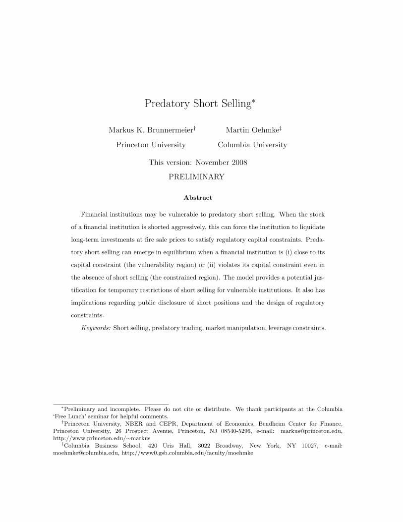
Lemma 1 implies that when the long-term investors offer a demand schedule to the short
sellers at t = 1, competition among short sellers will always ensure that the final price is
equal to fundamental value. This is illustrated in figure 1. The left panel shows the case in
which the intercept chosen by long-term investors is larger than the fundamental value of the
equity, i.e. P > XR−D0. In that case short sellers will take a short position S > 0, and since
competition ensures that short sellers will make zero profit in equilibrium, the equilibrium
short position S will be such the final price will be equal to fundamental, i.e. P = XR−D0.
The right panel shows the opposite case, in which the intercept chosen by the long-term
investors is below fundamental value. In that case short sellers end up taking a long position
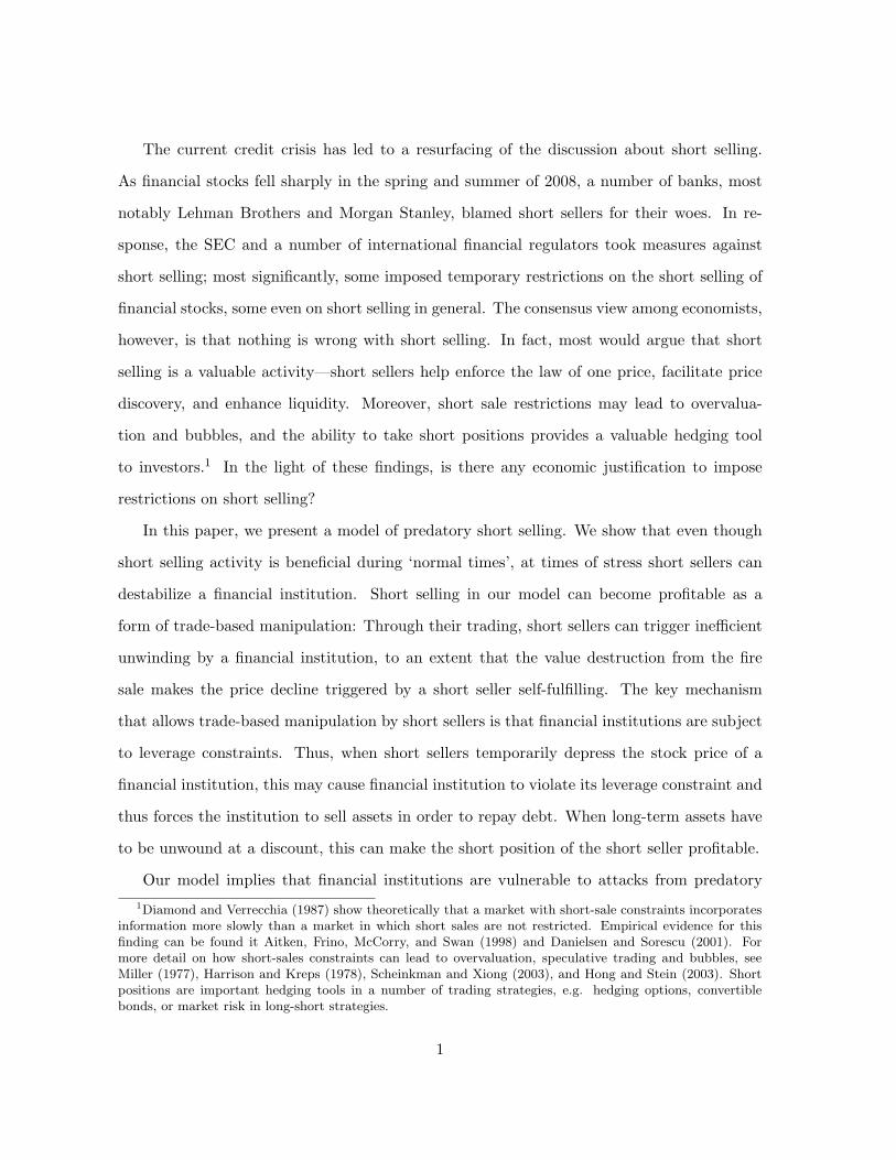
to ensure that the equity if fairly priced. Of course, when the intercept chosen by the is equal
to fundamental value, i.e. P = XR−D0, short sellers do not take a position in equilibrium,
i.e. S = 0. This is depicted in figure 2.
-10 0 10 20 30 40 50 60S
5
10
15
20
25
30
35
P, P�
P-ΛS
RX-D0
-10 0 10 20 30 40 50 60S
5
10
15
20
25
30
35
P, P�
P-ΛS
RX-D0
Figure 1: Impact of short selling without leverage constraint. In the left panel, the intercept chosenby long-term investors is larger than the fundamental value of equity, P > XR−D0. In that case short sellertake a short position ensuring that P = P − λS = XR − D0. In the right panel, the intercept is less thanfundamental value, such that the short sellers drive price up by taking a long position. The parameters in thisexample are: X = 10, R = 10, D = 68, λ = 0.75.
8
-10 0 10 20 30 40 50 60S
5
10
15
20
25
30
35
P, P�
P-ΛS
RX-D0
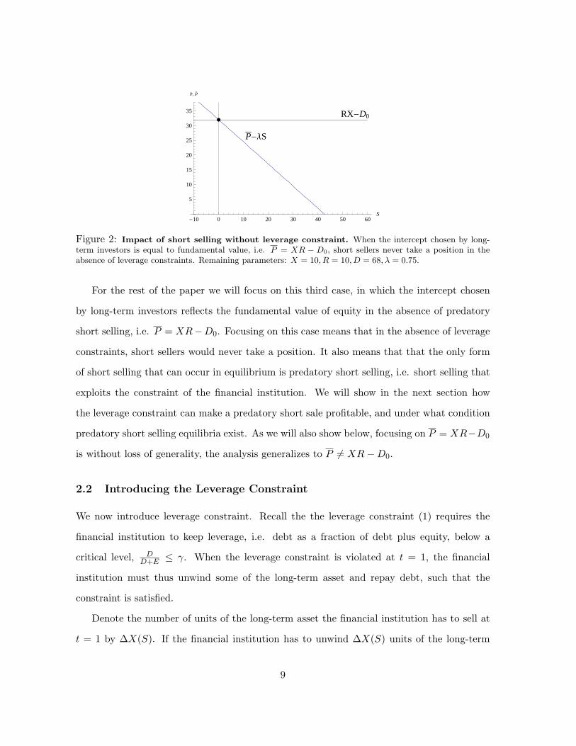
Figure 2: Impact of short selling without leverage constraint. When the intercept chosen by long-term investors is equal to fundamental value, i.e. P = XR − D0, short sellers never take a position in theabsence of leverage constraints. Remaining parameters: X = 10, R = 10, D = 68, λ = 0.75.
For the rest of the paper we will focus on this third case, in which the intercept chosen
by long-term investors reflects the fundamental value of equity in the absence of predatory
short selling, i.e. P = XR−D0. Focusing on this case means that in the absence of leverage
constraints, short sellers would never take a position. It also means that that the only form
of short selling that can occur in equilibrium is predatory short selling, i.e. short selling that
exploits the constraint of the financial institution. We will show in the next section how
the leverage constraint can make a predatory short sale profitable, and under what condition
predatory short selling equilibria exist. As we will also show below, focusing on P = XR−D0
is without loss of generality, the analysis generalizes to P 6= XR−D0.
2.2 Introducing the Leverage Constraint
We now introduce leverage constraint. Recall the the leverage constraint (1) requires the
financial institution to keep leverage, i.e. debt as a fraction of debt plus equity, below a
critical level, DD+E ≤ γ. When the leverage constraint is violated at t = 1, the financial
institution must thus unwind some of the long-term asset and repay debt, such that the
constraint is satisfied.
Denote the number of units of the long-term asset the financial institution has to sell at
t = 1 by ∆X(S). If the financial institution has to unwind ∆X(S) units of the long-term
9

asset at t = 1 to repay debt, this leads to an equity payout at time t = 2 of
P = max [XR−D0 − (1− δ)R∆X(S), 0] (4)
The reduction in equity value from unwinding, (1− δ)R∆X(S), stems from the fact that the
long-term asset can only be sold at a discount. Using equation (4) we can thus rewrite the
equilibrium conditions (3) as
P − λS = max [XR−D0 − (1− δ)R∆X(S), 0] . (5)
How much does the financial institution have to unwind? In order to find potential
equilibria, we need to determine how much the financial institution needs to unwind at
t = 1. To determine the value of ∆X(S), first notice that when the leverage constraint is not
violated at time t = 1, the financial institution does not have to unwind any of its long-term
investments. In that case, clearly ∆X(S) = 0.
What happens when the constraint is violated at t = 1 ? When the equity value at t = 1,
including the temporary price effects of short selling is such that the constraint is violated,
i.e.
D0
D0 + P − λS> γ,
the financial institution has to sell ∆X(S) units of the long-term asset and repay debt in order
to satisfy the constraint. The amount the financial institution has to unwind is determined
by the following condition:
D0 −∆X(S)δRD0 −∆X(S)δR + P − λS
= γ, (6)
which can be solved for ∆X(S). Combining the resulting expression with the facts that no
liquidation is necessary when the constraint is satisfied, and that the maximum amount that
10
can be liquidated is X, yields the following result:
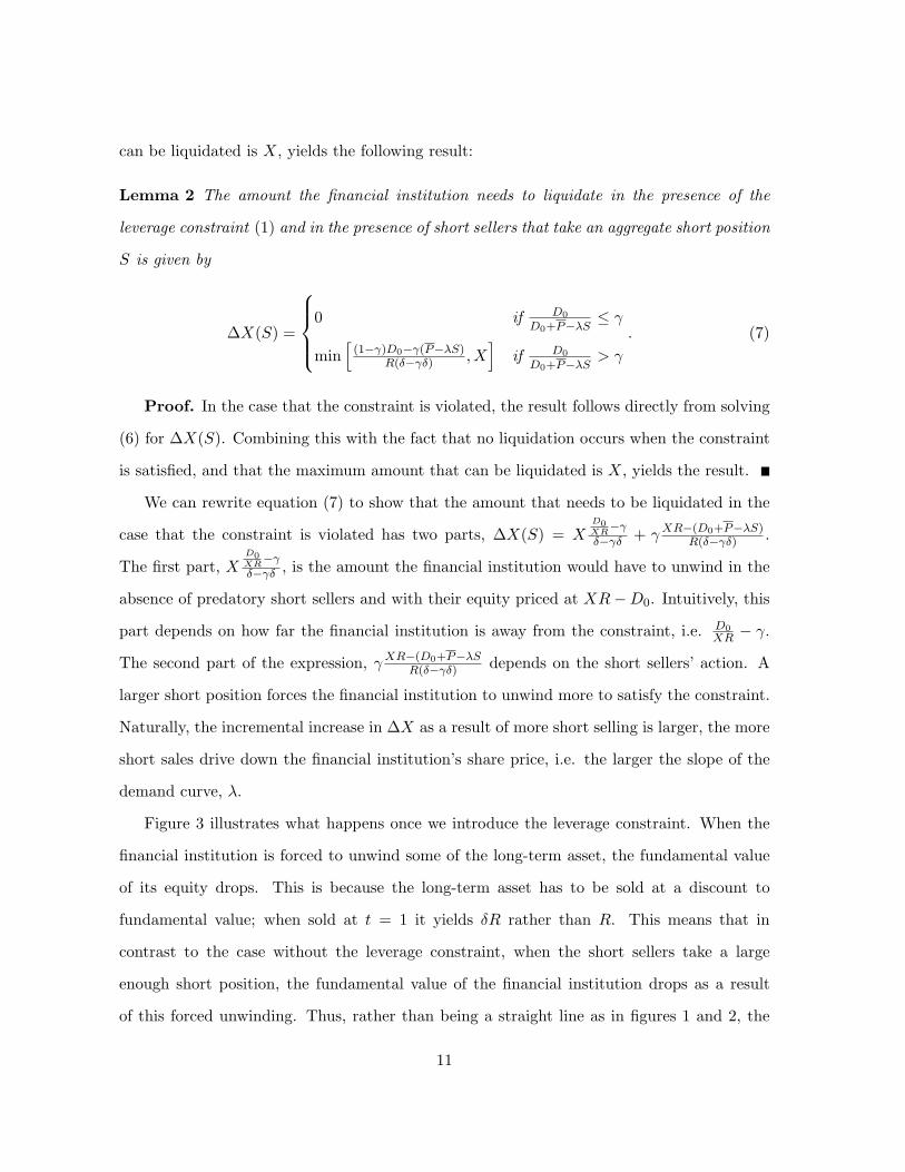
Lemma 2 The amount the financial institution needs to liquidate in the presence of the
leverage constraint (1) and in the presence of short sellers that take an aggregate short position
S is given by
∆X(S) =
0 if D0
D0+P−λS≤ γ
min[
(1−γ)D0−γ(P−λS)R(δ−γδ) , X
]if D0
D0+P−λS> γ
. (7)
Proof. In the case that the constraint is violated, the result follows directly from solving
(6) for ∆X(S). Combining this with the fact that no liquidation occurs when the constraint
is satisfied, and that the maximum amount that can be liquidated is X, yields the result.
We can rewrite equation (7) to show that the amount that needs to be liquidated in the
case that the constraint is violated has two parts, ∆X(S) = XD0XR
−γ
δ−γδ + γ XR−(D0+P−λS)R(δ−γδ) .
The first part, XD0XR
−γ
δ−γδ , is the amount the financial institution would have to unwind in the
absence of predatory short sellers and with their equity priced at XR−D0. Intuitively, this
part depends on how far the financial institution is away from the constraint, i.e. D0XR − γ.
The second part of the expression, γ XR−(D0+P−λSR(δ−γδ) depends on the short sellers’ action. A
larger short position forces the financial institution to unwind more to satisfy the constraint.
Naturally, the incremental increase in ∆X as a result of more short selling is larger, the more
short sales drive down the financial institution’s share price, i.e. the larger the slope of the
demand curve, λ.
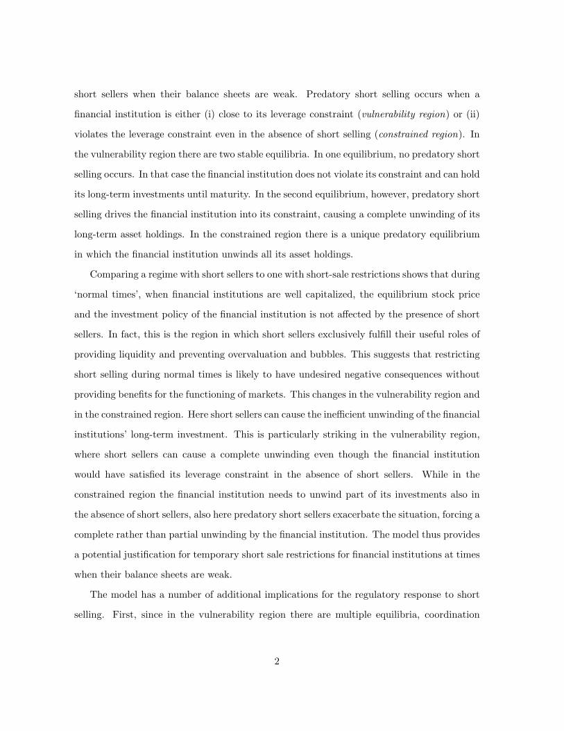
Figure 3 illustrates what happens once we introduce the leverage constraint. When the
financial institution is forced to unwind some of the long-term asset, the fundamental value
of its equity drops. This is because the long-term asset has to be sold at a discount to
fundamental value; when sold at t = 1 it yields δR rather than R. This means that in
contrast to the case without the leverage constraint, when the short sellers take a large
enough short position, the fundamental value of the financial institution drops as a result
of this forced unwinding. Thus, rather than being a straight line as in figures 1 and 2, the
11
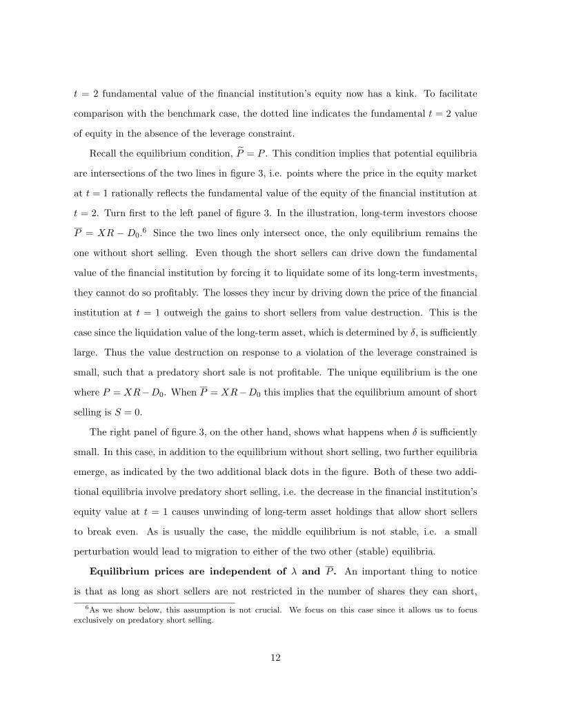
t = 2 fundamental value of the financial institution’s equity now has a kink. To facilitate
comparison with the benchmark case, the dotted line indicates the fundamental t = 2 value
of equity in the absence of the leverage constraint.
Recall the equilibrium condition, P = P . This condition implies that potential equilibria
are intersections of the two lines in figure 3, i.e. points where the price in the equity market
at t = 1 rationally reflects the fundamental value of the equity of the financial institution at
t = 2. Turn first to the left panel of figure 3. In the illustration, long-term investors choose
P = XR − D0.6 Since the two lines only intersect once, the only equilibrium remains the
one without short selling. Even though the short sellers can drive down the fundamental
value of the financial institution by forcing it to liquidate some of its long-term investments,
they cannot do so profitably. The losses they incur by driving down the price of the financial
institution at t = 1 outweigh the gains to short sellers from value destruction. This is the
case since the liquidation value of the long-term asset, which is determined by δ, is sufficiently
large. Thus the value destruction on response to a violation of the leverage constrained is
small, such that a predatory short sale is not profitable. The unique equilibrium is the one
where P = XR−D0. When P = XR−D0 this implies that the equilibrium amount of short
selling is S = 0.
The right panel of figure 3, on the other hand, shows what happens when δ is sufficiently
small. In this case, in addition to the equilibrium without short selling, two further equilibria
emerge, as indicated by the two additional black dots in the figure. Both of these two addi-
tional equilibria involve predatory short selling, i.e. the decrease in the financial institution’s
equity value at t = 1 causes unwinding of long-term asset holdings that allow short sellers
to break even. As is usually the case, the middle equilibrium is not stable, i.e. a small
perturbation would lead to migration to either of the two other (stable) equilibria.
Equilibrium prices are independent of λ and P . An important thing to notice
is that as long as short sellers are not restricted in the number of shares they can short,6As we show below, this assumption is not crucial. We focus on this case since it allows us to focus
exclusively on predatory short selling.
12

-10 0 10 20 30 40 50 60S
5
10
15
20
25
30
35
P, P�
P
P�
-10 0 10 20 30 40 50 60S
5
10
15
20
25
30
35
P, P�
P
P�
Figure 3: Introducing the leverage constraint. When the leverage constraint is introduced, a sufficientlylarge short position forces the financial institution to unwind. In the left panel the loss to the financialinstitution from unwinding the long asset is not large enough to make the short sale profitable (δ = 0.75).The only equilibrium is the one in which no short selling occurs. In the right panel, on the other hand, wesee that when the losses from liquidating the long-term asset are large enough two equilibria emerge withpositive amounts of short selling emerge in addition to the no-short-selling equilibrium (δ = 0.6). The middleequilibrium is unstable. The remaining parameters are: X = 10, R = 10, D = 68, λ = 0.75
the equilibrium prices are independent of the particular P and λ chosen by the long-term
investors. This means that while there are many equilibria with involving different combina-
tions of P , λ and S, the equilibria are isomorphic in terms of equilibrium prices. This means
that while focusing on P = XR−D0 allows us to focus exclusively on predatory short selling,
equilibrium prices and the existence of predatory short selling equilibria do not depend on
this assumption.
Lemma 3 When short sellers are unconstrained in the size of the short position they take,
the equilibrium prices and the amount that has to be unwound by the financial institution is
independent of λ and P .
Proof. This result comes from the fact that, in equilibrium, a change in either P or λ will
be exactly offset by a corresponding change in the equilibrium level of the short position S,
such that the equilibrium condition P = P is satisfied. Equilibrium prices and the equilibrium
amount that has to be unwound by the financial institution thus remain unaffected.
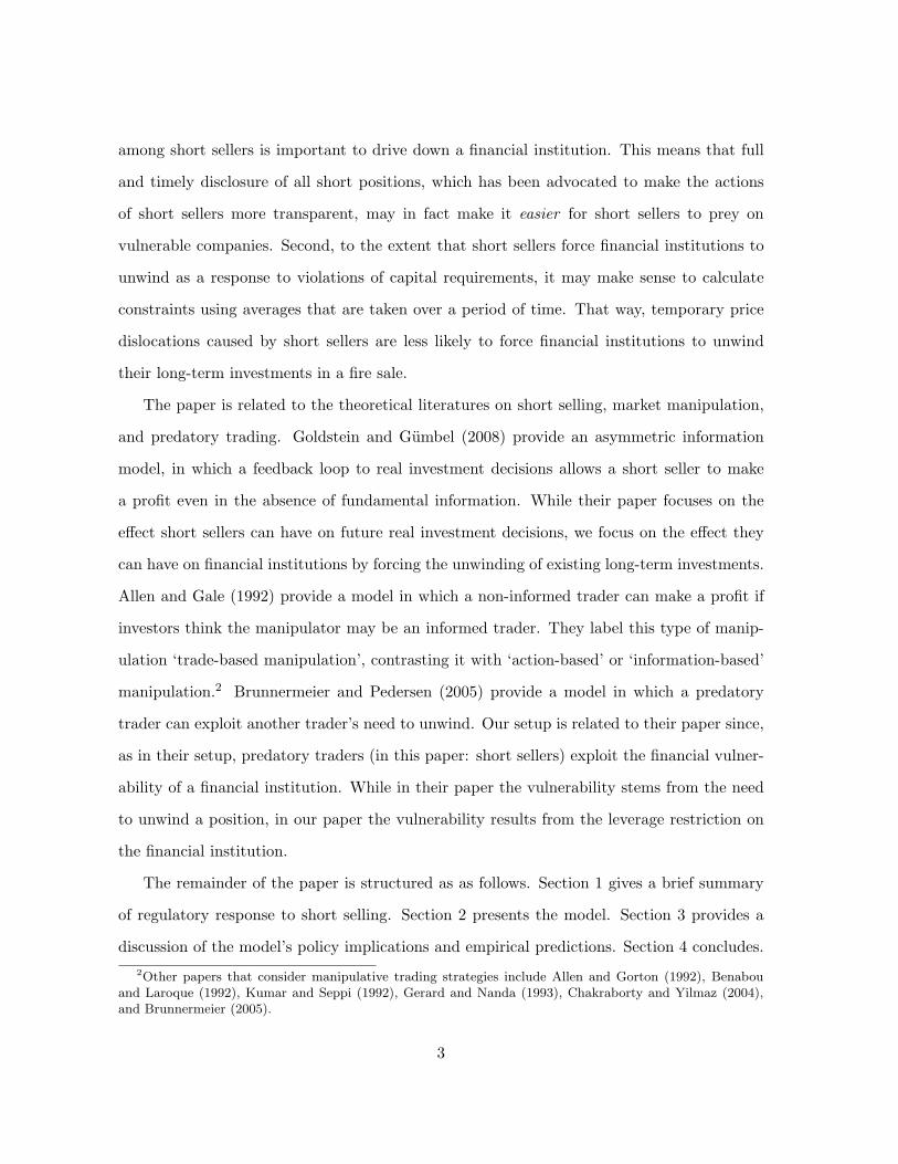
This independence result is illustrated in figure 4. Lemma 3 is convenient since it allows
us to classify equilibria by just looking at equilibrium prices and the amount of the long-term
13
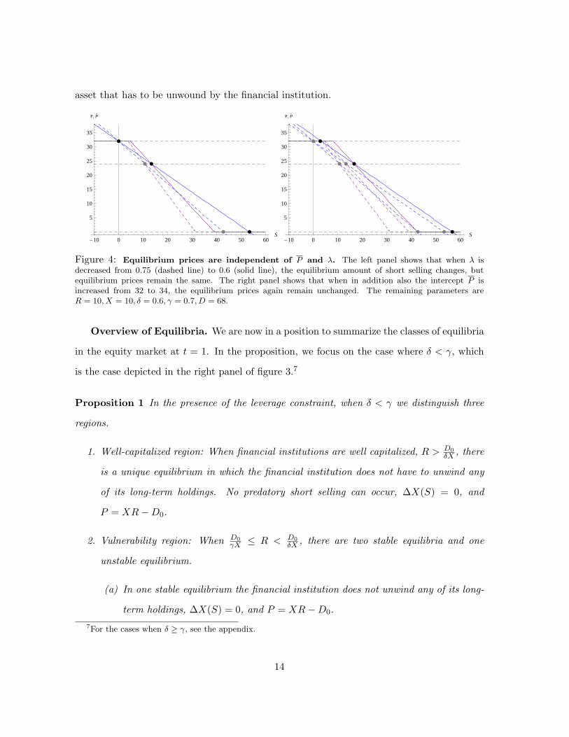
asset that has to be unwound by the financial institution.
-10 0 10 20 30 40 50 60S
5
10
15
20
25
30
35
P, P�
-10 0 10 20 30 40 50 60S
5
10
15
20
25
30
35
P, P�
Figure 4: Equilibrium prices are independent of P and λ. The left panel shows that when λ isdecreased from 0.75 (dashed line) to 0.6 (solid line), the equilibrium amount of short selling changes, butequilibrium prices remain the same. The right panel shows that when in addition also the intercept P isincreased from 32 to 34, the equilibrium prices again remain unchanged. The remaining parameters areR = 10, X = 10, δ = 0.6, γ = 0.7, D = 68.
Overview of Equilibria. We are now in a position to summarize the classes of equilibria
in the equity market at t = 1. In the proposition, we focus on the case where δ < γ, which
is the case depicted in the right panel of figure 3.7
Proposition 1 In the presence of the leverage constraint, when δ < γ we distinguish three
regions.
1. Well-capitalized region: When financial institutions are well capitalized, R > D0δX , there
is a unique equilibrium in which the financial institution does not have to unwind any
of its long-term holdings. No predatory short selling can occur, ∆X(S) = 0, and
P = XR−D0.
2. Vulnerability region: When D0γX ≤ R < D0
δX , there are two stable equilibria and one
unstable equilibrium.
(a) In one stable equilibrium the financial institution does not unwind any of its long-
term holdings, ∆X(S) = 0, and P = XR−D0.7For the cases when δ ≥ γ, see the appendix.
14

(b) In the other stable equilibrium the financial institution is forced to unwind its entire
holdings of the long-term asset, i.e. ∆X(S) = X and P = 0.
(c) In the unstable equilibrium the financial institution has to unwind part of its equity
holdings, ∆X(S) = Xγ− D0
XRγ−δ and P = 1−γ
γ−δ (D0 − δXR)
3. Constrained region: When R < D0γX , there is a unique equilibrium in which the financial
institution unwinds its entire holdings of the long-term asset, ∆X = X and P = 0.
Proof. See appendix.
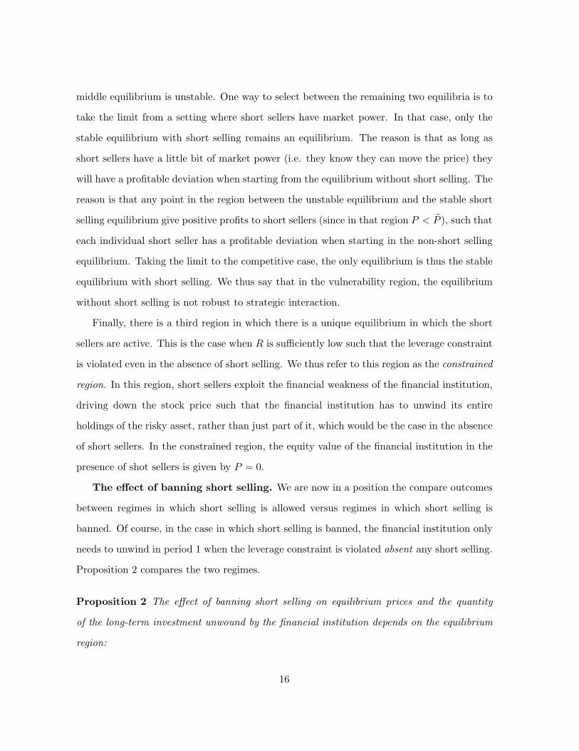
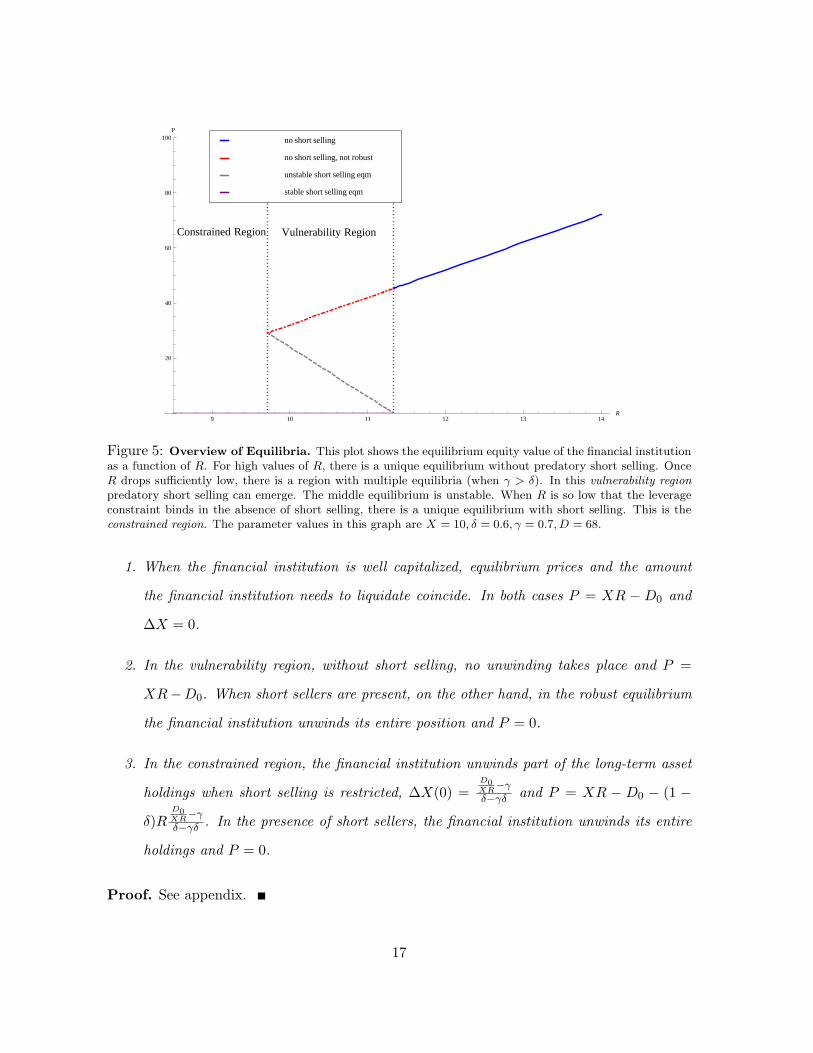
Figure 5 illustrates the equilibria as a function of R, the t = 1 expected payoff of the long-
term asset. As Proposition 1 points out, there are three regions of interest. First, when R is
sufficiently high, short sellers cannot profitably cause the financial institution to unwind. The
only equilibrium is the one in which the financial institution holds its long-term investments
until maturity. Expecting this, the equity value at t = 1 is given by XR−D0. We can think
of this region as characterizing the state in which financial institutions are healthy and well-
capitalized. When this is the case, short sellers play no role, except potentially fulfilling the
beneficial function of correcting the equity value of the financial institution when the long-
term investors (for some reason) offer an intercept that deviates from fundamental value.
Importantly, this means that when financial institutions are healthy, we should expect short
sellers to perform the beneficial tasks of price discovery and liquidity provision. We should
not, however, be concerned about predatory behavior by short sellers in this region.
However, when R drops sufficiently there is a second region with multiple equilibria. In
this region, the leverage constraint is satisfied if short sellers do not take any predatory short
positions that cause unwinding of the long-term asset. Thus, there is still an equilibrium
without short selling and without unwinding by the financial institution. However, there are
two equilibria in which short sellers take positions and force the financial institution to unwind
by driving it into the constraint. This means that in this region the financial institution is
vulnerable to short sellers, even though the leverage constraint is not binding. We thus refer
to this region of multiple equilibria as the vulnerability region. As is usually the case, the
15
middle equilibrium is unstable. One way to select between the remaining two equilibria is to
take the limit from a setting where short sellers have market power. In that case, only the
stable equilibrium with short selling remains an equilibrium. The reason is that as long as
short sellers have a little bit of market power (i.e. they know they can move the price) they
will have a profitable deviation when starting from the equilibrium without short selling. The
reason is that any point in the region between the unstable equilibrium and the stable short
selling equilibrium give positive profits to short sellers (since in that region P < P ), such that
each individual short seller has a profitable deviation when starting in the non-short selling
equilibrium. Taking the limit to the competitive case, the only equilibrium is thus the stable
equilibrium with short selling. We thus say that in the vulnerability region, the equilibrium
without short selling is not robust to strategic interaction.
Finally, there is a third region in which there is a unique equilibrium in which the short
sellers are active. This is the case when R is sufficiently low such that the leverage constraint
is violated even in the absence of short selling. We thus refer to this region as the constrained
region. In this region, short sellers exploit the financial weakness of the financial institution,
driving down the stock price such that the financial institution has to unwind its entire
holdings of the risky asset, rather than just part of it, which would be the case in the absence
of short sellers. In the constrained region, the equity value of the financial institution in the
presence of shot sellers is given by P = 0.
The effect of banning short selling. We are now in a position the compare outcomes
between regimes in which short selling is allowed versus regimes in which short selling is
banned. Of course, in the case in which short selling is banned, the financial institution only
needs to unwind in period 1 when the leverage constraint is violated absent any short selling.
Proposition 2 compares the two regimes.
Proposition 2 The effect of banning short selling on equilibrium prices and the quantity
of the long-term investment unwound by the financial institution depends on the equilibrium
region:
16
9 10 11 12 13 14R
20
40
60
80
100P
stable short selling eqm
unstable short selling eqm
no short selling, not robust
no short selling
Vulnerability RegionConstrained Region
Figure 5: Overview of Equilibria. This plot shows the equilibrium equity value of the financial institutionas a function of R. For high values of R, there is a unique equilibrium without predatory short selling. OnceR drops sufficiently low, there is a region with multiple equilibria (when γ > δ). In this vulnerability regionpredatory short selling can emerge. The middle equilibrium is unstable. When R is so low that the leverageconstraint binds in the absence of short selling, there is a unique equilibrium with short selling. This is theconstrained region. The parameter values in this graph are X = 10, δ = 0.6, γ = 0.7, D = 68.
1. When the financial institution is well capitalized, equilibrium prices and the amount
the financial institution needs to liquidate coincide. In both cases P = XR − D0 and
∆X = 0.
2. In the vulnerability region, without short selling, no unwinding takes place and P =
XR−D0. When short sellers are present, on the other hand, in the robust equilibrium
the financial institution unwinds its entire position and P = 0.
3. In the constrained region, the financial institution unwinds part of the long-term asset
holdings when short selling is restricted, ∆X(0) =D0XR
−γ
δ−γδ and P = XR − D0 − (1 −δ)R
D0XR
−γ
δ−γδ . In the presence of short sellers, the financial institution unwinds its entire
holdings and P = 0.
Proof. See appendix.
17

This is illustrated in figure 6. There are two important differences between the short selling
and no-short selling regimes. First, when short sales are restricted, there is no vulnerability
region. This means that the financial institution only has to unwind the long-term asset
when the leverage constraint is violated in absence of temporary price movements caused by
short sellers. Second, even when the constraint is violated in the absence of short selling, the
amount the financial institution has to unwind is (weakly) smaller than in the case with short
selling. This is the case since when the constraint is violated, short sellers always force the
financial institution to unwind its entire portfolio. When no short sellers are present, on the
other hand, the financial institution can in general satisfy the leverage constraint by selling
only part of its asset holdings, except when R drops so low that the financial institution
enters the ‘death spiral’, and has to unwind all its holdings even when no short sellers are
present. In the figure, this is the point where no short selling curve meets the x-axis.
Vulnerability RegionConstrained
RegionWell-capitalized
Region
9 10 11 12 13 14R
20
40
60
80
100P
Figure 6: The effect of banning short selling. This figure compares equilibria with and without shortsellers, focusing on robust, stable equilibria. When short selling is allowed, there is a discontinuous drop inprice as the financial institution enters the vulnerability region. Once in the vulnerability region, short sellersforce the financial institution to unwind its entire portfolio and P = 0. When short selling is not allowed, thefinancial institution does not have to unwind unless R drops far enough, even without short sellers present.Moreover, even in the region where the constraint is binding, the financial institution does not have to unwindits entire portfolio, except when its equity value truly hits zero. The parameter values in this graph areX = 10, δ = 0.6, γ = 0.7, D = 68.
18
The figure shows that when financial institutions are well-capitalized, the equilibria with
and without short selling coincide. Differences only occur once the financial institution enters
the vulnerability region or the constrained region. The difference is most notable in the
vulnerability region; once the financial institution is vulnerable, short seller can cause a
large, discontinuous drop in the equity value of the financial institution, together with the
inefficient unwinding of the entire position in the long-term asset. In this region, comparing
the financial institution’s equity value without short selling to the robust equilibrium8 with
short selling shows that short sellers reduce the equity value of the financial institution from
XR−D0 to 0. Total value of the financial institution is reduced by (1− δ)XR. Since short
sellers do not make a profit to offset this loss in value, this is an inefficiency.
In the constrained region the financial institution has to unwind some of the long-term
asset even in the absence of short seller. However, it can satisfy the leverage constraint by
selling strictly less when no short sellers are present. This is because short seller prey on
the weak financial institution by shorting its shares, forcing it to unwind even more of its
long-term investments. In fact, in the presence of short sellers, the only equilibrium in the
constrained region is the one in which the financial institution unwinds its entire portfolio
and the equity value is 0.
Regular selling vs. short selling. The analysis above has focused on predatory short
selling, rather than predatory selling. An important question is thus why predatory behavior
works through short selling, but not through regular selling. The reason is simple: a regular
seller cannot profit from this type of predatory behavior. Imagine a current owner of the
stock considering to sell the stock as the financial institution enters the vulnerability region.
Since the investor already owns the share, individually he has no incentive to drive down
the price through selling the stock. In other words, what makes predation possible is buying
back on the cheap after driving down the price. This means that in contrast to a short seller
who can make positive profits once the financial institution enters the vulnerability region,8We focus here on the robust equilibrium using the refinement explained above. Alternatively, without this
refinement, there is price multiplicity in this region and the equilibrium price will depend on which equilibriumshort sellers coordinate on.
19
an existing owner of the asset cannot make a profit and thus has no incentive to sell the share
to induce unwinding by the financial institution.9
3 Discussion
While the simple model presented above does not provide a fully-fledged welfare analysis of
short selling, the model generates a number of important insights that allow to devise a more
differentiated approach to regulating short selling than we have seen in the past. Below, we
briefly outline what we consider the main points regulators can take away from our analysis.
We also briefly discuss empirical predictions of the model.
Vulnerability of financial institutions. On of the main implications of the model is
that while short sellers are not able to prey on financial institutions when these are well-
capitalized, in times of stress it is possible that financial institutions become vulnerable
to predatory short sellers. The reason for this is that financial institutions face financing
constraints that allow short sellers to capitalize on financial weakness by forcing an institution
to unwind investments, leading to a reduction in fundamental value. This reduction in
fundamental value, in turn, makes the short sale profitable.
In terms of regulating short selling, the model thus implies that while banning short selling
during normal times is not desirable, it may make sense to restrict short selling temporarily
when financial institutions balance sheets are weak. The reason is that when banks are
well-capitalized (and predatory short selling does not occur in equilibrium) short sellers only
carry out their beneficial roles of enforcing the law of one price, providing liquidity and
incorporating information into prices. The model thus suggests that there is no justification
for a general ban of short selling on the grounds of predatory behavior. However, the model
does provide a potential justification for temporary restrictions of short selling. In particular,
when financial institutions’ balance sheets are weak and they enter the vulnerability region,9The only way in which an equilibrium similar to the predatory short selling equilibrium can occur through
regular selling is by coordination on a bad equilibrium: Regular owners may sell their shares because theysell everyone else to sell. This is comparable to the dominated equilibria in Diamond and Dybvig (1983) andBernardo and Welch (2004).
20
predatory short selling can be destabilizing, leading to negative skewness and inefficient
unwinding of long-term investments by the vulnerable institutions. While the paper does
not provide a full welfare analysis, this result provides a potential justification for temporary
short sales restrictions to curb predatory behavior.
Disclosure of short positions. Another important implication of the model is the
role of multiplicity in the vulnerability region. Since there are two stable equilibria in this
region, coordination among short sellers is crucial for which of the two equilibria we end
up in. This has important implications for the disclosure of short positions. In particular,
in addition to recent short-sale restrictions, a number of regulators have enacted tougher
disclosure requirements for short positions. In the US, the SEC now requires short sellers to
publicly disclose their positions weekly. In the UK, the FSA implemented a rule that requires
that investors disclose on each day any short positions in excess of 0.25% of the ordinary share
capital of financial companies at the end of trading the previous day. However, the results
from this model imply that this may, in fact, be counterproductive. In particular, requiring
public disclosure of all short positions may in fact facilitate coordination among predatory
short sellers. When short sellers are required to publicly disclose positions, it may thus be
more likely that we end up in the predatory equilibrium when in the vulnerability region.
This suggests that disclosure should either just be to the regulator, or should be made public
only with sufficient time delay.
Constraints based on averages. The model also has implications for the design of
regulatory constraints that financial institutions have to conform with. In particular, the
ability of the short sellers to prey on financial institution crucially depends on their ability
to move the financial institution’s constraint by temporarily driving down the stock price. In
the model, this is possible since the constraint is calculated using the current market price of
equity, which means that temporary price dislocations caused by short sellers are immediately
reflected in the financial institution’s constraint. A constraint that uses an average of past
prices taken over a certain period would weaken this link and make it harder for short sellers
21
to affect the financial institution’s constraint and cause unwinding.
Empirical predictions. The model predicts that large downward price movements
can occur when a financial institution enters the vulnerability region or the constrained
region. This means that in our model short selling increases negative skewness in equity
prices. This is opposite to the prediction in Hong and Stein (2003), whose model predicts
that banning short selling leads to negative skewness, and consistent with the empirical
evidence in Bris, Goetzmann, and Zhu (2007), who find evidence that there is significantly less
negative skewness in markets in which short selling is either not legal or not practiced. This
paper additionally predicts that in the cross-section, negative skewness should be observed
particularly for financial institutions with weak balance sheets, i.e. those that enter the
vulnerability region or the constrained region.
4 Conclusion
This paper provides a simple model of predatory short selling. Predatory short selling occurs
when short sellers exploit financial weakness or liquidity problems of a financial institution.
In our model, predatory short sales occur in equilibrium since the equity price drop caused
by the short sellers causes a leverage-constrained financial institution to unwind long-term
asset holdings at a discount. Predatory short selling only occurs when a financial institution
is either (i) close to its leverage constraint (vulnerability region) or (ii) violates the leverage
constraint even in the absence of short selling (constrained region). In the vulnerability
region there are two stable equilibria. In addition to an equilibrium without short selling,
there is a predatory equilibrium in which short sellers cause a complete unwinding of the
financial institution’s long-term asset holdings. In the constrained region there is a unique
predatory equilibrium in which the financial institution unwinds all its asset holdings. The
model provides a potential justification for temporary short sale restrictions for financial
institutions. Moreover, the model suggests that disclosure of short positions may facilitate
coordination among predatory short sellers, and that constraints of financial institutions
22

should be based on averages rather than snapshots.
5 Appendix
Proof of Proposition 1: First focus on the case when δ < γ. Intuitively, when δ < γ,
the P curve is steeper than the P curve, as depicted in the right panel of figure 3. We will
consider the three regions in turn. First, we compute the region in which no predatory short
selling can occur. Short sellers cannot succeed in predatory short selling when, after forcing
the financial institution to unwind the entire holdings of the long-term asset, the fundamental
value at t = 2 exceeds the price to which the short sellers need to drive the price to force the
unwinding. This is so because it means that short sellers have to buy back at a higher price
than they receive when selling the stock short.
To check this condition, assume that short sellers choose a short position S such that the
entire portfolio of the financial institution is liquidated, i.e. ∆X(S) = X. This requires that
(1− γ)D0 − γ(P − λS)R(δ − γδ)
= X (8)
which yields
S =γP + (1− γ)(δXR−D0)
λγ(9)
As pointed out above, this cannot be profitable when
XR−D0 − λS < δXR−D0 (10)
Using (9) to solve (10) for R yields
R >D0
δX, (11)
23

which is the expression in the proposition. This implies that the only equilibrium is the one
without predatory short selling, in which P = P = XR−D0.
Second, consider the region in which D0γX ≤ R < D0
δX . Note that in this region the leverage
constraint is not violated in the absence of predatory short selling, since DXR < γ. This means
that there is still an equilibrium in which no predatory short selling occurs and P = P =
XR−D0. However, from (11), we know that there is now also an equilibrium in which short
sellers force the financial institution to unwind its entire asset holdings. In this equilibrium,
by the zero profit condition, we have
P = XR−D0 − λS = max [δXR−D0, 0] = P. (12)
Since we know that in this region δXR −D0 < 0, we the equilibrium price must be P = 0.
Both of these equilibria are stable. Moreover, there is a third, unstable equilibrium, in which
only part of the financial institution’s investment is unwound. Denote the amount of short
selling in the unstable equilibrium by S∗. In this equilibrium, since ∆X(S∗) < X, we must
have
P − λS∗ = XR−D0 − (1− δ)∆X(S∗). (13)
Substituting in for ∆X(S∗) from equation (9) and solving for S∗ yields
S∗ =P
λ+
(1− γ)(δXR−D0
λ(γ − δ)(14)
Using this expression for S∗, we can determine the price in the unstable equilibrium as
P = P = P − λS∗ =1− γ
γ − δ(D − δXR). (15)
Substituting in to (9) yields that the amount the financial institution has to unwind in the
unstable equilibrium is ∆X(S∗) = Xγ− D0
XRγ−δ , as stated in the proposition.
24
Third, consider the region in which the leverage constraint is violated even in the absence
of predatory short selling, i.e DXR > γ. In this region, the equilibrium must involve short
selling to an extent that the entire portfolio of the financial institution is liquidated. The
reason is the following. Assume that DXR > γ. Absent short selling, the financial institution
would unwind an amount ∆X(0) such that the constraint is satisfied. This reduces the value
of the financial institution at t = 2 by (1− δ)∆X(0). This however implies that absent short
selling at t = 1, P = XR−D0 > XR−D0−(1−δ)∆X(0) = P . This means that short sellers
at t = 1 have an incentive to take a short position. This, in turn, exacerbates the leverage
constraint and forces the financial institution to unwind more. The only equilibrium is the
one where ∆X = X and P = P = 0. Intuitively, this is the case since the two lines cannot
intersect above the x-axis in this case; the P curve starts below the P curve, and is steeper,
such that the only intersections is on the flat part that lies on the x-axis.
Now consider what happens when δ > γ. Intuitively, when δ < γ, the P curve is less
steep than the P curve, as depicted in the left panel of figure 3. The first thing to note is that
now the vulnerability region disappears, since D0γX > D0
δX . In this case, as long as R > D0γX ,
the financial institution is well-capitalized and no predatory short selling occurs. As a result,
unwinding only takes place when R < D0γX . As before, when R < D0
γX , short sellers will be
active. When R > D0δX , short sellers force a partial unwinding of the financial institution’s
position in the long-term asset. When R < D0δX , short sellers force a complete unwinding.
Finally, in the knife-edge case when γ = δ, the P and P curves have the same slope.
This means that when R > D0γX predatory short selling cannot occur, while when R < D0
γX ,
the financial institution is unforced to unwind all its holdings and P = 0. When R = D0γX ,
the equilibrium price can lie on any point on the interval [0, XR −D0], as the two lines lie
directly on top of each other.
Proof of Proposition 2: We focus on the more interesting case when δ < γ. The price
in the presence of short sellers follows from proposition 1. The equilibrium t = 1 prices when
short selling is restricted are determined as follows. Assume that the long-term investors are
25
rational, such that they correctly anticipate the t = 2 payoff XR − D0 − (1 − δ)R∆X(0).
As long as the leverage constraint is not violated, i.e. DXR < γ, the financial institution
does not have to liquidate, and P = XR −D0. When DXR > γ, the financial institution has
to unwind ∆X(0) = XD0XR
−γ
δ−γδ units of the long-term asset, yielding an equilibrium price of
P = XR−D0− (1− δ)XRD0XR
−γ
δ−γδ . When δ > γ, the plot would look similar, but there would
be no vulnerability region, and in part of the constrained region the financial institutions
equity value would still be positive, since only a part of the long-term asset gets unwound.
References
Aitken, Michael J., Alex Frino, Michael S. McCorry, and Peter L. Swan, 1998, Short sales are
almost instantaneously bad news: Evidence from the australian stock exchange, Journal
of Finance 53, 2205–2223.
Allen, Franklin, and Douglas Gale, 1992, Stock-price manipulation, Review of Financial
Studies 5, 503–529.
Allen, Franklin, and Gary Gorton, 1992, Stock price manipulation, market microstructure
and asymmetric information, European Economic Review 36, 624–630.
Benabou, Roland, and Guy Laroque, 1992, Using privileged information to manipulate mar-
kets: Insiders, gurus, and credibility, Quarterly Journal of Economics 107, 921–958.
Bernardo, Antonio E., and Ivo Welch, 2004, Liquidity and financial market runs, Quarterly
Journal of Economics 119, 135–158.
Bris, Arturo, William N. Goetzmann, and Ning Zhu, 2007, Efficiency and the bear: Short
sales and markets around the world, Journal of Finance 62, 1029–1079.
Brunnermeier, Markus K., 2005, Information leakage and market efficiency, Review of Finan-
cial Studies 18, 417–457.
26
, and Lasse H. Pedersen, 2005, Predatory trading, The Journal of Finance 60, 1825–
1863.
Chakraborty, Debasish, and Bilge Yilmaz, 2004, Informed manipulation, Journal of Economic
Theory 114, 132–152.
Danielsen, Bartley R., and Sorin M. Sorescu, 2001, Why do option introductions depress stock
prices? a study of diminishing short sale constraints, Journal of Financial and Quantitative
Analysis 36, 451–484.
Diamond, Douglas W., and Philip H. Dybvig, 1983, Bank runs, deposit insurance, and liq-
uidity, Journal of Political Economy 91, 401–419.
Diamond, Douglas W., and Robert E. Verrecchia, 1987, Constraints on short-selling and asset
price adjustment to private information, Journal of Financial Economics 18, 277–311.
Gerard, Bruno, and Vikram Nanda, 1993, Trading and manipulation around seasoned equity
offerings, The Journal of Finance 48, 213–245.
Goldstein, Itay, and Alexander Gumbel, 2008, Manipulation and the allocational role of
prices, Review of Economic Studies 75, 133–164.
Harrison, J. Michael, and David M. Kreps, 1978, Speculative investor behavior in a stock
market with heterogeneous expectations, Quarterly Journal of Economics 92, 323–336.
Hong, Harrison, and Jeremy C. Stein, 2003, Differences of opinion, short-sales constraints
and market crashes, Review of Fiancial Studies 16, 487–525.
Kumar, Praveen, and Duane J. Seppi, 1992, Futures manipulation with ”cash settlement”,
Journal of Finance 47, 1485–1502.
Kyle, Albert S., 1985, Continuous auctions and insider trading, Econometrica 53, 1315–1335.
Miller, Edward M., 1977, Risk, uncertainty, and divergence of opinion, Journal of Finance
32, 1151–1168.
27
Scheinkman, Jose A., and Wei Xiong, 2003, Overconfidence and speculative bubbles, Journal
of Political Economy 111, 1183–1219.
28