preconditioned multigrid methods for compressible flow

JOURNAL OF COMPUTATIONAL PHYSICS 136, 425–445 (1997)ARTICLE NO. CP975772

Preconditioned Multigrid Methods for Compressible FlowCalculations on Stretched Meshes

Niles A. Pierce and Michael B. Giles

Oxford University Computing Laboratory, Numerical Analysis Group, Oxford OX1 3QD, United KingdomE-mail: [email protected]

Received April 29, 1996; revised May 29, 1997

whelming. On the other hand, the development of efficientnumerical methods for solution of the Navier–Stokes equa-Efficient preconditioned multigrid methods are developed for

both inviscid and viscous flow applications. The work is motivated tions remains one of the ongoing challenges in the fieldby the mixed results obtained using the standard approach of scalar of computational fluid dynamics. Dramatic improvementspreconditioning and full coarsened multigrid, which performs well over the performance of existing methods will be necessaryfor Euler calculations on moderately stretched meshes but is far

before this area of research may be considered satisfacto-less effective for turbulent Naiver–Stokes calculations, when the cellstretching becomes severe. In the inviscid case, numerical studies rily resolved.of the preconditioned Fourier footprints demonstrate that a block- The difficulty for viscous calculations stems from theJacobi matrix preconditioner substantially improves the damping need to use a computational mesh that is highly resolvedand propagative efficiency of Runge–Kutta time-stepping schemes

in the direction normal to the wall in order to accuratelyfor use with full coarsened multigrid, yielding computational sav-represent the steep gradients in the boundary layer. Theings of approximately a factor of three over the standard approach.

In the viscous case, determination of the analytic expressions for resulting high aspect ratio cells greatly reduce the efficiencythe preconditioned Fourier footprints in an asymptotically stretched of existing numerical algorithms. The design of an appro-boundary layer cell reveals that all error modes can be effectively priate numerical approach must therefore be based on adamped using a combination of block-Jacobi preconditioning and

careful assessment of the interaction between the discretea J-coarsened multigrid strategy, in which coarsening is performedonly in the direction normal to the wall. The computational savings method, the computational mesh, and the physics of theusing this new approach are roughly a factor of 10 for turbulent viscous flow.Navier–Stokes calculations on highly stretched meshes. Q 1997 Aca- Since the relevant problem size will continue to increasedemic Press

as fast as hardware constraints will allow, it is critical thatthe convergence rate of the method should be insensitiveto the number of unknowns. The general solution strategy1. INTRODUCTIONthat appears most promising in this regard is multigrid,for which grid-independent convergence rates have beenIn broad terms, the field of computational fluid dynamicsproven for elliptic operators [1–5]. Although no rigoroushas developed in response to the need for accurate, effi-extension of this theory has emerged for problems involv-cient, and robust numerical algorithms for solving increas-

ingly complete descriptions of fluid motion over increasing a hyperbolic component, methods based on multigridhave proven highly effective for inviscid calculations withingly complex flow geometries. The present work focuses

entirely on the efficiency aspects of this pursuit for the two the Euler equations [6–8] and remain the most attractiveapproach for Navier–Stokes calculations despite thesystems of governing equations that have been of principle

interest during the last two decades: the Euler equations, widely observed performance breakdown in the presenceof boundary layer anisotropy.describing inviscid rotational compressible flow and the

Reynolds averaged Navier–Stokes equations (supple- In the present work, steady solutions to the Euler andNavier–Stokes equations are obtained by time-marchingmented with an appropriate turbulence model), describing

viscous turbulent compressible flow. There is a significant the unsteady systems until the time-derivative terms havebecome sufficiently small to ensure the desired degree ofdisparity in the degree to which existing methods have so

far succeeded in producing efficient solutions to these two steadiness in the solution. Numerically, a steady state isachieved by eliminating transient error modes either bysystems of equations. On the one hand, techniques devel-

oped for the Euler equations are already relatively effec- damping or by expulsion from the computational domain.Since the transient solution is not of interest, multigrid cantive, so that while both the need and opportunity for further

improvement are significant, they do not appear over- be employed to accelerate convergence to a steady state

4250021-9991/97 $25.00

Copyright 1997 by Academic PressAll rights of reproduction in any form reserved.

426 PIERCE AND GILES

without concern for the loss of time-accuracy. Classicalmultigrid techniques developed for elliptic problems trans-fer the low frequency errors in the solution to a successionof coarser meshes where they become high frequency er-rors that are more effectively smoothed by traditional re-laxation methods. For the unsteady Euler and Navier–Stokes equations, which exhibit both parabolic andhyperbolic properties in their discrete formulations, thecoarse meshes in the multigrid cycle serve the dual role ofenhancing both damping and propagation of error modes.Since damping is essentially a local process and error expul-sion a global one (requiring disturbances to propagateacross the domain to a far field boundary), it is the dampingproperties of the relaxation scheme that are most criticalto ensuring insensitivity to problem size. The propagative

FIG. 1. Diagnosis of multigrid breakdown for the Euler and Navier–efficiency of the relaxation method remains important toStokes equations.the performance of the multigrid algorithm, but it is none-

theless a second priority during the investigations thatfollow.

Efficient multigrid performance hinges on the ability of large stability limits along the imaginary and negative realaxes. Explicit multigrid solvers based on this approachthe relaxation scheme to eliminate on the current mesh

all modes that cannot be resolved without aliasing on the represent an important schematic innovation in enablinglarge and complex Euler calculations to be performed asnext coarser mesh in the cycle. The choice between an

explicit or an implicit relaxation scheme to drive the a routine part of the aerodynamic design procedure [7, 8].However, despite the favorable convergence rates ob-multigrid algorithm requires consideration of the computa-

tional trade-offs, in addition to the relative damping and served for Euler computations, this approach does notsatisfy all the requirements for efficient multigrid perfor-propagative efficiencies of the approaches. Explicit

schemes offer a low operation count, low storage require- mance. These shortcomings become far more evident whenthe approach is applied to Navier–Stokes calculations.ments, and good parallel scalability, but they suffer from

the limited stability imposed by the CFL condition. Alter- The hierarchy of factors leading to multigrid inefficiencyare illustrated in Fig. 1. The two fundamental causes ofnatively, implicit schemes theoretically offer unconditional

stability but are more computationally intensive, require degraded multigrid performance for both the Euler andNavier–Stokes equations are stiffness in the discrete sys-a heavy storage overhead, and are more difficult to paral-

lelize efficiently. In practice, direct inversion is infeasible tem and decoupling of modes in one or more coordinatedirections. These two problems manifest themselves in anfor large problems due to a high operation count, so that

some approximate factorization such as ADI or LU must identical manner by causing the corresponding residualeigenvalues to fall near the origin in the complex plane sobe employed. The resulting factorization errors effectively

limit the convergence of the scheme when very large time that they can be neither damped nor propagated efficientlyby the multistage relaxation scheme. For Euler computa-steps are employed so that it is not possible to fully capital-

ize on the potential benefits of unconditional stability. tions, discrete stiffness results primarily from the use of ascalar preconditioner (local time step) [11], which is unableGiven these circumstances, it therefore seems advanta-

geous to adopt an explicit approach if a scheme with suit- to cope with the inherent disparity in the propagativespeeds of convective and acoustic modes. This problem isable properties can be designed.

A popular explicit multigrid smoother is the semi-dis- relatively localized for transonic flows since the stiffnessis only substantial near the stagnation point, at shocks,crete scheme proposed by Jameson et al. [9] which uses

multistage Runge–Kutta time-stepping to integrate the and across the sonic line. Directional decoupling in Eulercomputations results primarily from alignment of the flowo.d.e. resulting from the spatial discretization. In accor-

dance with the requirements for efficient multigrid perfor- with the computational mesh, which causes some convec-tive modes to decouple in the transverse direction. Al-mance, the coefficients of the Runge–Kutta scheme are

chosen to promote rapid damping and propagation of error though improvements are possible, these shortcomingshave not prevented the attainment of sufficiently rapidmodes [7, 10]. This is accomplished by ensuring that the

amplification factor is small in regions of the complex plane convergence to meet industrial requirements for inviscidflow calculations [12] and do not represent a substantialwhere the residual eigenvalues corresponding to high fre-

quency modes are concentrated, as well as by providing concern to the CFD community.

PRECONDITIONED MULTIGRID METHODS 427

For Navier–Stokes computations, the problems re- relaxation scheme must eliminate all high frequencymodes, and also those modes that are high frequency insulting from the disparity in propagative speeds and from

flow alignment still persist, but a far more serious source one mesh direction and low frequency in the other. Foruse in conjunction with an explicit Runge–Kutta scheme,of difficulties is introduced by the high aspect ratio cells

inside the boundary layer. These highly stretched cells Allmaras recommends an implicit ADI preconditioner be-cause explicit methods are notoriously poor at dampingincrease the discrete stiffness of the system by several or-

ders of magnitude so that the entire convective Fourier modes with a low frequency component [26]. Buelow etal. [28] have employed a related strategy based on a differ-footprints collapse to the origin while decoupling the

acoustic modes from the streamwise coordinate direction. ent local matrix preconditioner [29] and ADI relaxation.Alternatively, the semi-coarsening algorithm proposedUnder these circumstances, the multigrid algorithm is ex-

tremely inefficient at eliminating a large fraction of the by Mulder [27] coarsens separately in each mesh directionand therefore reduces the region of Fourier space for whicherror modes which could potentially exist in the solution.

Convergence problems for Navier–Stokes applications the relaxation scheme on each mesh must successfullydamp error modes. To obtain an O(N) method for a three-are also compounded by the need to incorporate a turbu-

lence model. Popular algebraic models are notorious for dimensional calculation in which N is the cost of a singlefine mesh evaluation, Mulder defined a restriction andintroducing a disruptive blinking phenomenon into the

convergence process as the reference distance migrates prolongation structure in which not all grids are coarsenedin every direction. For two-dimensional grids that areback and forth between neighboring cells. Alternatively,

adopting a one- or two-equation model requires solution of coarsened separately in both directions, only those modesthat are high frequency in both mesh directions need beturbulent transport equations that incorporate production

and destruction source terms that are both temperamental damped by the relaxation scheme. For this purpose, All-maras suggests the point-implicit block-Jacobi precondi-and stiff. However, recent efforts have demonstrated that

turbulent transport equations can be successfully discret- tioner proposed by Morano et al. [19] that has previouslybeen demonstrated to be effective in clustering high fre-ized using a multigrid approach without interfering with

the convergence process of the flow equations [13, 14]. quency eigenvalues away from the origin [21]. For gridsthat are not coarsened in one of the mesh directions, All-One means of combatting discrete stiffness in the Euler

and Navier–Stokes equations is the use of a matrix time maras proposes using a semi-implicit line-Jacobi precondi-tioner in that direction [26].step or preconditioner [15, 11, 16–20]. In the present work,

the preconditioner is viewed as a mechanism for overcom- These strategies for preconditioning in the context ofboth full and semi-coarsened multigrid are well-conceived.ing discrete stiffness by clustering the residual eigenvalues

away from the origin into a region of the complex plane The drawback to implicit preconditioning for full coars-ened multigrid is the associated increase in operationfor which the multistage scheme can provide rapid damping

and propagation [21, 22]. This is an alternative viewpoint count, storage overhead, and difficulty in efficient paralleli-zation. The drawback to a semi-coarsened approach is pri-to the one invoked by those who have developed precondi-

tioners for low-Mach number and incompressible flows [15, marily the increase in operation count: for a three-dimen-sional computation, the costs for full coarsened V- and W-23–25], where the focus is placed on eliminating analytic

stiffness arising from the inherent propagative disparities cycles are bounded by LjN and FdN, respectively, while forsemi-coarsening, the cost of a V-Cycle is bounded by 8Nin the limit of vanishing Mach number. In certain cases,

preconditioning methods can also be used to alleviate the and a W-cycle is no longer O(N) [27].The purpose of the present work is to analyze and imple-problem of directional decoupling [22, 14, 26]. Another

method for countering directional decoupling is the use ment two less expensive preconditioned multigrid methodsthat are designed to perform efficiently for Euler and tur-of directional coarsening multigrid algorithms [27]. The

interaction between the preconditioner and the multigrid bulent Navier–Stokes calculations, respectively. In the caseof the Euler equations, existing multigrid solvers em-coarsening algorithm is critical, making it imperative that

the two components of the scheme are considered simulta- ploying a standard scalar preconditioner [11] and a fullcoarsened strategy routinely demonstrate relatively goodneously when attempting to design efficient preconditioned

multigrid methods. convergence rates [12] despite their failure to satisfy allthe damping and propagation requirements for efficientAllmaras provided a systematic examination of the

damping requirements for relaxation methods used in con- multigrid performance. The widespread success using thisapproach suggests that the computational challenges aris-junction with both the traditional full coarsened multigrid

and for the semi-coarsening multigrid algorithm of Mulder ing from discrete stiffness and directional decoupling arenot particularly severe for Euler calculations. Therefore,[26, 27]. Using full coarsened multigrid in two dimensions,

only modes which are low frequency in both mesh direc- it is undesirable to pursue alternative methods that incura substantial increase in the cost and complexity of eachtions can be resolved on the coarser grids, so that the


multigrid cycle in order to ensure that these efficiency sional calculations. The improved preconditionedmultigrid methods have also been incorporated success-criteria are completely satisfied. Instead, it seems reason-

able to view these efficiency requirements as a worthwhile fully into other research projects that rely on a steadystate solver as an inner kernel. These include both optimalobjective to be attained to the highest degree possible while

maintaining the desirable cost and complexity properties design by adjoint methods [31, 32] and unsteady simula-tions based on an inner multigrid iteration [33–35].of a full coarsened approach. Numerical studies of the

preconditioned Fourier footprints are used to demonstratethat substantial improvements in full coarsened multigrid 2. APPROACHperformance can be achieved by replacing the standard

2.1. Scheme Descriptionscalar preconditioner with the block-Jacobi matrix precon-ditioner proposed by Morano et al. [19] and suggested by Construction and analysis of the proposed methods pro-Allmaras for use with the more expensive semi-coarsened ceeds from the two-dimensional linearized Navier–Stokesstrategy [26]. For Euler calculations on typical inviscid equations in Cartesian coordinatesmeshes, the new approach of matrix preconditioning andfull coarsened multigrid yields computational savings ofroughly a factor of three over the standard combination W

t1 A

Wx

1 BWy

5 C2Wx2 1 D

2Wy2 1 E

2Wx y

,of scalar preconditioning and full coarsened multigrid[22, 14].

where W is the state vector, A and B are the inviscid fluxThe development of an efficient preconditionedJacobians, and C, D, and E are the viscous flux Jacobians.multigrid method for turbulent Navier–Stokes calculationsA preconditioned semi-discrete finite volume discretiza-represents a far more demanding challenge since existingtion of this system appears asmethods have proven largely inadequate for coping with

the problems arising from highly stretched boundary layerLtW 1 PR(W) 5 0, (1)cells. To identify the specific nature of these problems and

assist in designing an inexpensive algorithm that does notfalter in the presence of boundary layer anisotropy, the where R(W) is the residual vector of the spatial discretiza-present work examines the analytic form of the two-dimen- tion, Lt represents the multistage Runge–Kutta operatorsional preconditioned Fourier footprints inside an asymp- and P is the preconditioner, which has the dimension oftotically stretched boundary layer cell [22, 14]. This analysis time and plays the role of a time step. The transient solutionreveals the asymptotic dependence of the residual eigen- is not of interest for steady applications so the precondi-values on the two Fourier angles, thus exposing the cluster- tioner and the coefficients of the Runge–Kutta operatoring properties of the preconditioned algorithm. In particu- can be chosen to promote rapid convergence without re-lar, it is demonstrated that the balance between streamwise gard for time-accuracy. The steady solution admitted byconvection and normal diffusion inside the boundary layer the spatial discretization is unaffected by the choice ofenables a point-implicit block-Jacobi preconditioner to en- preconditioner as long as P is nonsingular since the systemsure that even those convective modes with a low frequency reduces to R(W) 5 0 when the unsteady terms have van-component in one mesh direction are effectively damped ished.[22]. A simple modification of the full coarsened algorithm For the analysis that follows, R is taken to be the stan-to a J-coarsened strategy, in which coarsening is performed dard linear operatoronly in the direction normal to the wall, further ensuresthat all acoustic modes are damped [14]. Therefore, it is

R 5A

2 Dxd2x 2

uAu2 Dx

dxx 1B

2 Dyd2y 2

uBu2 Dy

dyynot necessary to resort to either an implicit preconditioneror a complete semi-coarsening algorithm to produce a pre- (2)conditioned multigrid method that effectively damps all 2

CDx2 dxx 2

DDy2 dyy 2

E4 Dx Dy

d2x2y ,modes. For the computation of two-dimensional turbulentNavier–Stokes flows, this combination of block-Jacobi pre-conditioning and J-coarsened multigrid yields computa- where upwinding of the inviscid terms is accomplished by

a Roe linearization [36]. Numerical dissipation of this typetional savings of roughly an order of magnitude over ex-isting methods that rely on the standard combination of corresponds to a matrix dissipation [37], in which each

characteristic field is upwinded by introducing dissipationfull coarsened multigrid with a scalar preconditioner.This new preconditioned multigrid method has recently scaled by the associated characteristic speed. A related

form of scalar dissipation is obtained by replacing uAu andbeen extended to three-dimensional turbulent Navier–Stokes calculations [30] and has been shown to provide uBu in (2) by their spectral radii r(A) and r(B), so that the

dissipation for each characteristic is instead scaled by theessentially the same convergence rates as for two-dimen-


maximum characteristic speed [9]. This approach is less conditioner is defined by the purely hyperbolic time step,P21

SE5 Dt21

H , assuming that the numerical dissipation intro-expensive since it avoids matrix operations, but it is alsoless accurate as it introduces unnecessarily large amounts duced to prevent oscillations is sufficiently small so as not

to limit the stability. The implications of this assumptionof dissipation into all but one of the characteristic fields.The implications for stability and convergence are com- for the scaling of the numerical dissipation are examined

in Section 2.4.pared for these two alternative schemes, but detailed analy-sis will focus on the more accurate matrix dissipation ap-

2.3. Matrix Preconditionerproach.Assuming constant Pr and c, the four independent pa- The matrix preconditioner used for the present work is

rameters that govern the discrete Navier–Stokes residual a point-implicit block-Jacobi preconditioner [19, 21] thatare the cell Reynolds number, Mach number, cell aspect is obtained from the discrete residual operator (2) by ex-ratio, and flow angle: tracting the terms corresponding to the central node in

the stencil

ReDx 5u Dx

n, M 5

Ïu2 1 v2

c,

DyDx

,vu

.

P21MNS

51

CFLHSuAu

Dx1

uBuDy

12CDx2 1

2DDy2D.

A Cartesian mesh is assumed to simplify notation, but thetheory extends naturally to real applications using either

The corresponding form of the matrix preconditioner forstructured or unstructured meshes.the Euler equations is obtained by eliminating the vis-cous contributions2.2. Scalar Preconditioner

A conservative time step estimate for the Navier–StokesP21

ME5

1CFLH

SuAuDx

1uBuDyD.equations is based on the purely hyperbolic and parabolic

time steps formed using the spectral radii of the flux Jacobi-ans [38],

It has been demonstrated in Ref. [14] that the precondi-tioner takes a fundamentally similar form for a 2nd/4th

Dt21NS 5 Dt21

H 1 Dt21P , difference switched JST scheme [9] based on the same Roe

linearization [36]. This compatibility and related numericalwhere the hyperbolic time step is given by experiments suggest that it is acceptable to base the pre-

conditioner on a first-order discretization even when usinghigher order switched and limited schemes.

Dt21H 5

1CFLH

Sr(A)Dx

1r(B)Dy D

2.4. Stability Considerations

and the parabolic time step is It is essential to note that the choice of either a scalaror matrix preconditioner cannot be made independentlyfrom the choice of numerical dissipation. This may be

Dt21P 5

1CFLP

S4r(C)Dx2 1

4r(D)Dy2 1

r(E)Dx DyD. understood by considering the necessary and sufficient

stability condition for the scalar convection–diffusionequation,The factor of 4 in the parabolic time step arises from

considering the worst-case scenario of a checkerboardut 1 aux 5 nuxx ,mode, Wi, j 5 W

`̀

(t)eı̂(fi1fj), for which the coefficients of thesecond-difference stencil reinforce each other in both di-

discretized using central differences in space and forwardrections. The hyperbolic and parabolic CFL numbers,differences in time,CFLH and CFLP , reflect the extent of the stability region

of the Runge–Kutta time-stepping scheme along the imagi-nary and negative real axes, respectively. In comparison Dt # min S2n

a2 ,Dx2

2n D.with a uniform global time step, this local stability estimatedefines a suitable scalar preconditioner for the Navier–Stokes equations, P21

SNS5 Dt21

NS , that reduces stiffness re- This discretization can be used to represent first-order up-winding of a scalar convection equation if the diffusionsulting from variation in spectral radius and cell size

throughout the mesh [11]. coefficient is chosen to correspond to the appropriate formof numerical dissipation n 5 uauDx/2. In this case, the stabil-For the Euler equations, the corresponding scalar pre-


ity requirement then reduces to the standard CFL condi- flow on a mesh with constant spacing and periodic bound-ary conditions. The validity of the analysis then dependstion Dt # Dx/uau.

The corresponding representation of the Euler equa- on the degree to which the true local behavior of thesolution can be modeled under these assumptions. Numeri-tions with characteristic-based matrix dissipation iscal results for both the Euler and Navier–Stokes equationsindicate that Fourier analysis does provide a useful indica-

Wt 1 AWx 5Dx2

uAuWxx . tor of scheme performance characteristics.In the context of a semi-discrete scheme (1), the Fourier

footprint of the spatial discretization is critical in revealingThe one-dimensional system can be decoupled into scalarthe effectiveness of the Runge–Kutta time-steppingcharacteristic equations,scheme in damping and propagating error modes. Thefootprint is found by substituting a semi-discrete Fourier

Vt 1 LVx 5Dx2

uLuVxx , mode of the form

Wi, j 5 W`̀

(t)eı̂(iux1juy)using an eigenvector decomposition of the flux JacobianA 5 TLT21 to produce the characteristic variables V 5

into the discrete residual operator (2). The Fourier ampli-T21W, where L is a diagonal eigenvalue matrix. Applyingtude W

`̀

(t) satisfies the evolution equationthe convection–diffusion stability requirement separatelyto each characteristic equation leads to the limit Dtk #

LtW`̀

1 PZW`̀

5 0,Dx/ulku for the kth characteristic, where lk is the corre-sponding eigenvalue. The scalar preconditioner is stable

where Z is the Fourier symbol of the residual operator:but suboptimal since all characteristics evolve with Dtk 5Dx/maxk(ulku). The matrix preconditioner is stable and alsooptimal in one dimension, since Dtk 5 Dx/ulku, and each Z(ux , uy) 5 ı̂

ADx

sin ux 1uAuDx

(1 2 cos ux)characteristic wave is evolving at its stability limit.

The Euler equations with standard scalar dissipation1 ı̂

BDy

sin uy 1uBuDy

(1 2 cos uy)take the form

12CDx2 (1 2 cos ux) 1

2DDy2 (1 2 cos uy)Wt 1 AWx 5

Dx2

r(A)Wxx ,

1E

Dx Dysin ux sin uy .where r(A) is the spectral radius of the flux Jacobian. This

system can still be decoupled into characteristic equationsusing the same transformation as above. However, the The Fourier footprint is defined by the eigenvalues ofstability requirement for all characteristics is now just the the matrix PZ, which are functions of the Fourier anglesstandard scalar CFL condition, Dtk # Dx/r(A). As a result, ux and uy . For stability, the footprint must lie within thethe matrix preconditioner is unstable when used in con- stability region of the time-stepping scheme specified byjunction with scalar dissipation based on the spectral radius uc(z)u # 1, where uc(z)u is the amplification factor de-and only the scalar preconditioner is appropriate. Out of fined bythe four possible combinations of scalar and matrix precon-ditioner and numerical dissipation, the three stable combi- W

`̀n11 5 c(z)W

`̀n.

nations are denoted PSRM , PMRM , and PSRS . The behaviorof the scalar preconditioner applied to scalar dissipation The stability region and contours for a 5-stage Runge–(PSRS) will only be considered briefly to illuminate the Kutta scheme due to Martinelli [38] are shown in Fig. 2properties of the other two combinations since it produces to provide a realistic context for eigenvalue clustering.a different steady state solution and it is undesirable to In two dimensions, there are four characteristic familiescompromise accuracy for the purposes of convergence. representing convective entropy modes, convective vortic-

ity modes and two groups of acoustic pressure modes.2.5. Fourier Footprints

From a damping perspective, it is desirable for the residualeigenvalues corresponding to all these modes to be clus-To assess the properties of the proposed methods, Fou-

rier analysis is used to decompose the error into modal tered into a region of the complex plane where the amplifi-cation factor is significantly less than unity. The primarycomponents which can then be examined individually. This

analytic approach is based on a local linearization of the weakness of explicit time integration using a scalar time


sion of these error modes will also enhance the perfor-mance of the multigrid algorithm. Analysis of eigenvalueclustering will initially focus on modes that are high fre-quency in both mesh directions (Hx Hy) since point-implicitmethods are notoriously poor at eliminating modes witha low frequency component.

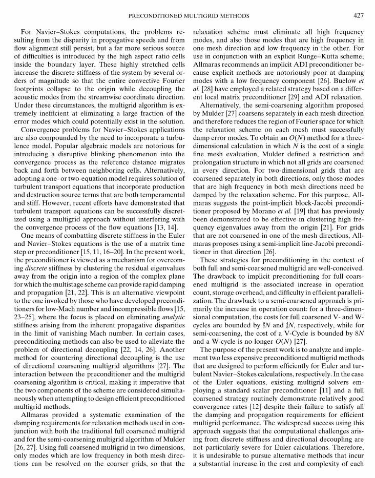
High Frequency Modes. Fourier footprints corre-sponding to high frequency modes for aligned inviscid sub-sonic flow in a moderately stretched mesh cell are shownfor all three stable combinations of preconditioner andnumerical dissipation in Fig. 4. The outer solid line in theseplots is the stability region of the time-stepping schemewhich must contain all the residual eigenvalues to ensurestability. The fact that the maximum extent along the nega-tive real axis is roughly twice the extent in either directionalong the imaginary axis suggests the definition CFLP 52CFLH , so that only the hyperbolic CFL number need bedetermined and the subscript may be dropped. The innersolid line represents the envelope of all possible high fre-FIG. 2. Stability region and contours defined by uc(z)u 5 0.1, 0.2, ...,

1.0 for a 5-stage Runge–Kutta time-stepping scheme. quency footprints arising from a related scalar model prob-lem preconditioned by a suitable scalar time step [21].Since scalar preconditioning is entirely appropriate for ascalar problem, this boundary represents a useful clusteringstep is that a significant fraction of the residual eigenvaluestarget for a matrix preconditioner applied to a system ofcluster near the origin where the amplification factor isequations. For the purposes of the discussion that follows,close to unity and the damping of error modes is verythis boundary will be considered to define the optimalinefficient. Since, at the origin, the gradient vector of theclustering envelope from a damping perspective. From aamplification factor lies along the negative real axis, im-propagative viewpoint, only the curved portion of theproved damping of these troublesome modes will followboundary is optimal.directly from an increase in the magnitude of the real

component of the corresponding residual eigenvalues.Error modes are propagated at the group velocity corre-

sponding to a discrete wave packet of the correspondingspatial frequency. Since the expression for the group veloc-ity depends on the form of the temporal discretizationoperator Lt , it is not possible to determine detailed propa-gative information from the Fourier footprint. However,for Runge–Kutta operators of the type used in the presentwork, the group velocity corresponding to a given residualeigenvalue is related to the variation in the imaginary com-ponents of all the residual eigenvalues in that modal family[39]. Therefore, for rapid propagation, it is desirable forthe residual eigenvalues in each family to extend far fromthe negative real axis.

3. ANALYSIS

3.1. Preconditioned Multigrid for the Euler Equations

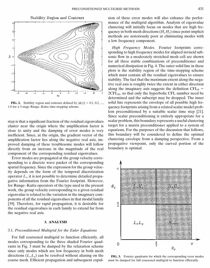
For full coarsened multigrid to function efficiently, allmodes corresponding to the three shaded Fourier quad-rants in Fig. 3 must be damped by the relaxation schemesince only modes which are low frequency in both meshdirections (Lx Ly) can be resolved without aliasing on the FIG. 3. Fourier quadrants for which the corresponding error modes

must be damped for full coarsened multigrid to function efficiently.coarse mesh. Efficient propagation and subsequent expul-


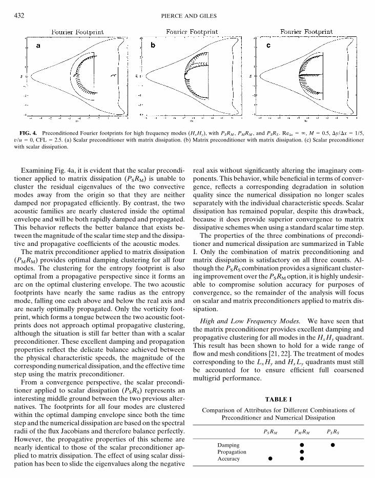
FIG. 4. Preconditioned Fourier footprints for high frequency modes (HxHy), with PSRM , PMRM , and PSRS . ReDx 5 y, M 5 0.5, Dy/Dx 5 1/5,v/u 5 0, CFL 5 2.5. (a) Scalar preconditioner with matrix dissipation. (b) Matrix preconditioner with matrix dissipation. (c) Scalar preconditionerwith scalar dissipation.

Examining Fig. 4a, it is evident that the scalar precondi- real axis without significantly altering the imaginary com-ponents. This behavior, while beneficial in terms of conver-tioner applied to matrix dissipation (PSRM) is unable to

cluster the residual eigenvalues of the two convective gence, reflects a corresponding degradation in solutionquality since the numerical dissipation no longer scalesmodes away from the origin so that they are neither

damped nor propagated efficiently. By contrast, the two separately with the individual characteristic speeds. Scalardissipation has remained popular, despite this drawback,acoustic families are nearly clustered inside the optimal

envelope and will be both rapidly damped and propagated. because it does provide superior convergence to matrixdissipative schemes when using a standard scalar time step.This behavior reflects the better balance that exists be-

tween the magnitude of the scalar time step and the dissipa- The properties of the three combinations of precondi-tioner and numerical dissipation are summarized in Tabletive and propagative coefficients of the acoustic modes.

The matrix preconditioner applied to matrix dissipation I. Only the combination of matrix preconditioning andmatrix dissipation is satisfactory on all three counts. Al-(PMRM) provides optimal damping clustering for all four

modes. The clustering for the entropy footprint is also though the PSRS combination provides a significant cluster-ing improvement over the PSRM option, it is highly undesir-optimal from a propagative perspective since it forms an

arc on the optimal clustering envelope. The two acoustic able to compromise solution accuracy for purposes ofconvergence, so the remainder of the analysis will focusfootprints have nearly the same radius as the entropy

mode, falling one each above and below the real axis and on scalar and matrix preconditioners applied to matrix dis-sipation.are nearly optimally propagated. Only the vorticity foot-

print, which forms a tongue between the two acoustic foot-High and Low Frequency Modes. We have seen that

prints does not approach optimal propagative clustering,the matrix preconditioner provides excellent damping and

although the situation is still far better than with a scalarpropagative clustering for all modes in the Hx Hy quadrant.

preconditioner. These excellent damping and propagationThis result has been shown to hold for a wide range of

properties reflect the delicate balance achieved betweenflow and mesh conditions [21, 22]. The treatment of modes

the physical characteristic speeds, the magnitude of thecorresponding to the Lx Hy and Hx Ly quadrants must still

corresponding numerical dissipation, and the effective timebe accounted for to ensure efficient full coarsened

step using the matrix preconditioner.multigrid performance.

From a convergence perspective, the scalar precondi-tioner applied to scalar dissipation (PSRS) represents aninteresting middle ground between the two previous alter- TABLE Inatives. The footprints for all four modes are clustered Comparison of Attributes for Different Combinations ofwithin the optimal damping envelope since both the time Preconditioner and Numerical Dissipationstep and the numerical dissipation are based on the spectral

PS RM PM RM PS RSradii of the flux Jacobians and therefore balance perfectly.However, the propagative properties of this scheme are

Damping d dnearly identical to those of the scalar preconditioner ap-Propagation d

plied to matrix dissipation. The effect of using scalar dissi- Accuracy d dpation has been to slide the eigenvalues along the negative


FIG. 5 Preconditioned Fourier footprints for all modes except LxLy using first-order upwind matrix dissipation. ReDx 5 y, M 5 0.5, Dy/Dx 5

1/5, v/u 5 0, CFL 5 2.5. (a) Scalar preconditioner. (b) Matrix preconditioner.

For Euler calculations, the cell stretching is typically not switching from full coarsened multigrid to a more expen-sive algorithm.severe so that discrete stiffness is chiefly caused by the

inherent disparity in propagative speeds and directional3.2. Preconditioned Multigrid for the

decoupling results primarily from flow alignment, as pre-Navier–Stokes Equations

viously indicated in Fig. 1. Propagative disparities are mostpronounced near the stagnation point, across the sonic The situation is much different for turbulent Navier–

Stokes calculations, where the highly stretched boundaryline, and at shocks, while flow alignment results near theairfoil surface when using a body-conforming mesh. layer cells significantly exacerbate both the stiffness and

decoupling problems. Convergence degrades rapidly as theIn regions of strong propagative disparity or perfect flowalignment, neither preconditioner succeeds in clustering cell aspect ratios increase, so for viscous applications it is

essential to account for the damping of every error mode.all of the eigenvalues corresponding to the Lx Hy and Hx Ly

quadrants away from the origin. However, there is a quali- Although it is optimal if modes are both rapidly dampedand propagated, in the demanding context of severetative difference in the magnitude of this shortcoming, as

illustrated by the footprints in Fig. 5 which contain the boundary layer anisotropy, the clustering is deemed suc-cessful as long as the eigenvalues do not cluster arbitrarilyresidual eigenvalues corresponding to all modes except

those in the Lx Ly quadrant for the same aligned subsonic close to the origin where the amplification factor is unity.The most effective means of understanding the phenom-flow conditions as were previously considered. Using the

scalar preconditioner, the entire footprints of both convec- enon of multigrid breakdown is an examination of theform of the preconditioned residual eigenvalues in a highlytive families are densely clustered near the origin so that

both damping and propagation are impeded. With the ma- stretched boundary layer cell. For this purpose, the analyticexpressions for the preconditioned Fourier footprints aretrix preconditioner, only the tips of the two convective

footprints touch the origin and the rest of the eigenvalues obtained for the important set of asymptotic limits summa-rized in Table II. Cases E1 and E2 represent the inviscidin these families extend far away from both the real axis

and the origin. As a result, those modes clustered near flows corresponding to the viscous conditions of cases NS1and NS2, and are provided to illustrate the importance ofthe origin which cannot be effectively damped will still

propagate relatively efficiently in the streamwise direction viscous coupling across the boundary layer in determiningthe appropriate course of action. Case 1 represents asince the associated group velocity is proportional to the

maximum imaginary component achieved by any of the stretched cell with perfect flow alignment while Case 2corresponds to the same stretched cell with diagonal crosseigenvalues in that family. For typical inviscid computa-

tions, the impact on convergence of the few troublesome flow. For the viscous cases, the cell aspect ratio is scaled toreflect the physical balance between streamwise convectionsawtooth modes that are not well damped using the matrix

preconditioner is almost certainly insufficient to warrant and normal diffusion, so that


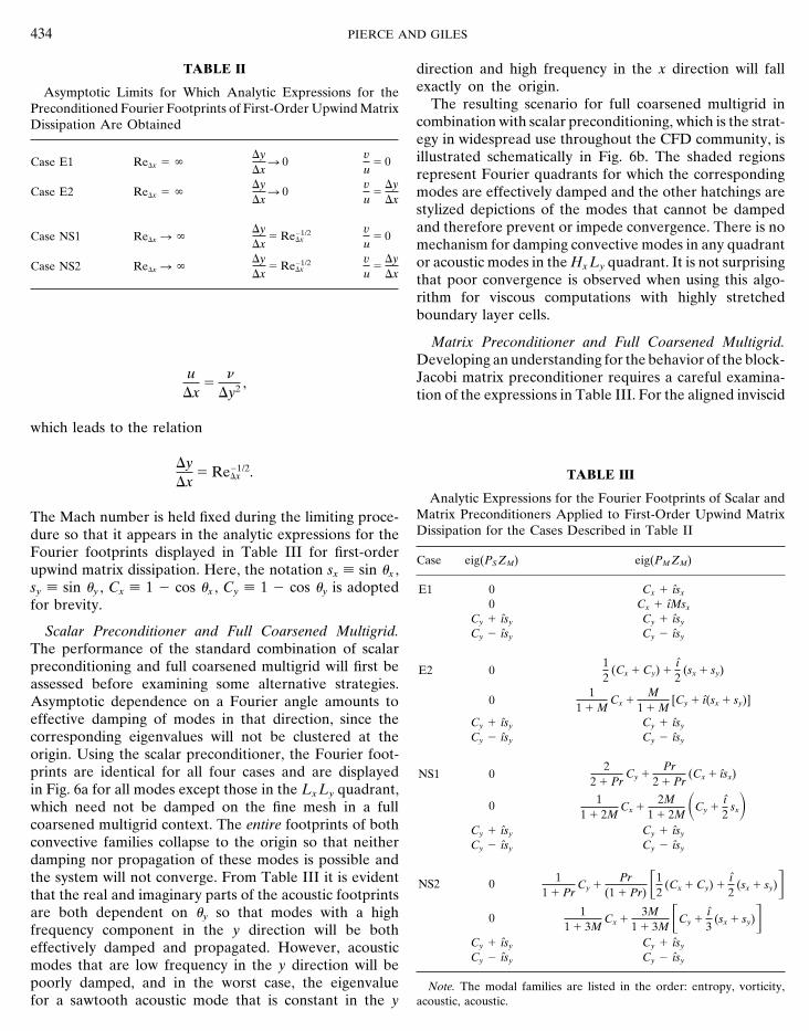
TABLE II direction and high frequency in the x direction will fallexactly on the origin.Asymptotic Limits for Which Analytic Expressions for the

The resulting scenario for full coarsened multigrid inPreconditioned Fourier Footprints of First-Order Upwind Matrixcombination with scalar preconditioning, which is the strat-Dissipation Are Obtainedegy in widespread use throughout the CFD community, isillustrated schematically in Fig. 6b. The shaded regionsDy

DxR 0

vu

5 0Case E1 ReDx 5 yrepresent Fourier quadrants for which the corresponding

DyDx

R 0vu

5DyDx

Case E2 ReDx 5 y modes are effectively damped and the other hatchings arestylized depictions of the modes that cannot be dampedand therefore prevent or impede convergence. There is noDy

Dx5 Re21/2

Dxvu

5 0Case NS1 ReDx R ymechanism for damping convective modes in any quadrantor acoustic modes in the Hx Ly quadrant. It is not surprisingDy

Dx5 Re21/2

Dxvu

5DyDx

Case NS2 ReDx R ythat poor convergence is observed when using this algo-rithm for viscous computations with highly stretchedboundary layer cells.

Matrix Preconditioner and Full Coarsened Multigrid.Developing an understanding for the behavior of the block-Jacobi matrix preconditioner requires a careful examina-u

Dx5

nDy2 ,

tion of the expressions in Table III. For the aligned inviscid

which leads to the relation

DyDx

5 Re21/2Dx . TABLE III

Analytic Expressions for the Fourier Footprints of Scalar andMatrix Preconditioners Applied to First-Order Upwind MatrixThe Mach number is held fixed during the limiting proce-Dissipation for the Cases Described in Table IIdure so that it appears in the analytic expressions for the

Fourier footprints displayed in Table III for first-orderCase eig(PS ZM) eig(PM ZM)

upwind matrix dissipation. Here, the notation sx ; sin ux ,sy ; sin uy , Cx ; 1 2 cos ux , Cy ; 1 2 cos uy is adopted E1 0 Cx 1 ı̂sx

0 Cx 1 ı̂Msxfor brevity.Cy 1 ı̂sy Cy 1 ı̂sy

Scalar Preconditioner and Full Coarsened Multigrid. Cy 2 ı̂sy Cy 2 ı̂sy

The performance of the standard combination of scalarpreconditioning and full coarsened multigrid will first be 1

2(Cx 1 Cy) 1

ı̂2

(sx 1 sy)E2 0assessed before examining some alternative strategies.

11 1 M

Cx 1M

1 1 M[Cy 1 ı̂(sx 1 sy)]0Asymptotic dependence on a Fourier angle amounts to

effective damping of modes in that direction, since the Cy 1 ı̂sy Cy 1 ı̂sy

Cy 2 ı̂sy Cy 2 ı̂sycorresponding eigenvalues will not be clustered at theorigin. Using the scalar preconditioner, the Fourier foot-prints are identical for all four cases and are displayed 2

2 1 PrCy 1

Pr2 1 Pr

(Cx 1 ı̂sx)NS1 0in Fig. 6a for all modes except those in the Lx Ly quadrant,

0 11 1 2M

Cx 12M

1 1 2M SCy 1ı̂2

sxDwhich need not be damped on the fine mesh in a fullcoarsened multigrid context. The entire footprints of both Cy 1 ı̂sy Cy 1 ı̂syconvective families collapse to the origin so that neither Cy 2 ı̂sy Cy 2 ı̂sy

damping nor propagation of these modes is possible andthe system will not converge. From Table III it is evident NS2 0 1

1 1 PrCy 1

Pr(1 1 Pr) F1

2(Cx 1 Cy) 1

ı̂2

(sx 1 sy)Gthat the real and imaginary parts of the acoustic footprintsare both dependent on uy so that modes with a high 0 1

1 1 3MCx 1

3M1 1 3M FCy 1

ı̂3

(sx 1 sy)Gfrequency component in the y direction will be both

Cy 1 ı̂sy Cy 1 ı̂syeffectively damped and propagated. However, acousticCy 2 ı̂sy Cy 2 ı̂symodes that are low frequency in the y direction will be

poorly damped, and in the worst case, the eigenvalue Note. The modal families are listed in the order: entropy, vorticity,acoustic, acoustic.for a sawtooth acoustic mode that is constant in the y


FIG. 6. Clustering performance of the scalar preconditioner and implications for full coarsened multigrid inside a highly stretched bound-ary layer cell with aligned flow. Footprint symbols: entropy (1), vorticity (?), acoustic (p, s). (a) Fourier footprint for all modes except LxLy .(b) Damping schematic for full coarsened multigrid.

flow of Case E1, the convective modes are dependent only AGARD Case 6 calculation [14]. Figure 7a reveals thatthe entropy footprint is clustered well away from the originon ux , and the acoustic modes are dependent only on uy ,

so that each modal family is effectively damped in only for all modes. The vorticity footprint remains distinctlyclustered away from the origin even at this low Mach num-two Fourier quadrants. By comparison, the viscous results

of Case NS1 reveal that the balance between streamwise ber. Propagative clustering of the vorticity mode away fromthe real axis improves if either the Mach number or theconvection and normal diffusion has caused the two con-

vective families to become dependent on both Fourier flow angle increases.This beneficial effect on the clustering of the convectiveangles, so that all quadrants except Lx Ly will be effectively

damped. For the entropy family, this property is indepen- eigenvalues has a profound influence on the outlook forthe performance of full coarsened multigrid as describeddent of Mach number, while for the vorticity family, this

behavior exists except in the case of vanishing Mach num- in Fig. 7b. Darker shading is used to denote the Fourierquadrants for which damping is facilitated by use of aber. For both inviscid and viscous results, the effect of

introducing diagonal cross flow in Case 2 is to improve matrix preconditioner. The full coarsened algorithm willnow function efficiently for all convective modes. However,the propagative performance for the convective modes by

introducing a dependence on both Fourier angles in the the footprints for the acoustic modes still approach theorigin when uy is small, so the only remaining impedimentsimaginary components. Notice that the matrix precondi-

tioner has no effect on the footprints for the acoustic to efficient performance are the acoustic modes corre-sponding to the Hx Ly quadrant.modes, which are identical to those using the scalar precon-

ditioner.The scenario for full coarsened multigrid using the ma- Matrix Preconditioner and J-Coarsened Multigrid. The

fact that the block-Jacobi preconditioner provides effectivetrix preconditioner is illustrated by the Fourier footprintand schematic damping diagram of Fig. 7. The footprint clustering of convective eigenvalues in all but the Lx Ly

quadrant provides the freedom to modify the multigriddepicts all modes except Lx Ly for the perfectly alignedviscous flow of Case NS1 with M 5 0.04. This Mach number coarsening strategy with only the damping of Hx Ly acoustic

modes in mind. One possibility that avoids the high cost ofrepresents a realistic value for a highly stretched boundarylayer cell at the wall, the specific value being observed at a complete semi-coarsening stencil and takes advantage of

the damping properties revealed in the present analysis is athe mid-chord for a cell with y1 , 1 in an RAE2822


FIG. 7. Clustering performance of the block-Jacobi matrix preconditioner and implications for full coarsened multigrid inside a highly stretchedboundary layer cell with aligned flow. Footprint symbols: entropy (1), vorticity (?), acoustic (p, s). (a) Footprint for all modes except LxLy . CaseNS1 with M 5 0.04. (b) Damping schematic for full coarsened multigrid.

J-coarsened strategy in which coarsening is performed only the preconditioner and multigrid algorithm is critical, sincethe preconditioner is chiefly responsible for damping thein the direction normal to the wall. The implications for

multigrid performance with this approach are summarized convective modes and the coarsening strategy is essentialto damping the acoustic modes.in Fig. 8. The Fourier footprint is plotted for the diagonal

cross flow of Case NS2 with M 5 0.2 to demonstrate the Cost bounds for full and J-coarsened cycles are pre-sented in Table IV, where N is the cost of a single flowrapid improvement in the clustering of the convective eigen-

values as the flow angle and Mach number increase above evaluation on the fine mesh. The cost of J-coarsenedmultigrid is independent of the number of dimensions sincethe extreme conditions shown in Fig. 7a. Only residual ei-

genvalues corresponding to modes in the Lx Hy and Hx Hy coarsening is performed in only one direction. For aV-cycle, the cost of J-coarsening is 80% more than fullFourier quadrants are displayed in Fig. 8a since modes from

the other two quadrants can be resolved on the next coarser coarsening in two dimensions and 133% more in threedimensions. Use of a J-coarsened W-cycle is inadvisablemesh. The residual eigenvalues are now effectively clus-

tered away from the origin for all families. since the cost depends on the number of multigrid levels(K). While there is a significant overhead associated withThe schematic of Fig. 8b demonstrates that the combina-

tion of block-Jacobi preconditioning and J-coarsened using J-coarsened vs. full coarsened multigrid, subsequentdemonstrations will show that the penalty is well worth-multigrid accounts for the damping of all error modes

inside highly stretched boundary layer cells. This result while for turbulent Navier–Stokes calculations.Implementation for structured grid applications isholds even for the perfectly aligned flow of Case NS1 as

long as the Mach number does not vanish. The requirement straightforward for single block codes but problematic formulti-block solvers. Coarsening directions will not neces-on Mach number emphasizes the point that the methods

developed in this paper are not intended for precondi- sarily coincide in all blocks so that cell mismatches wouldbe produced at the block interfaces on the coarse meshes.tioning in the limit of incompressibility. For typical viscous

meshes, the Mach number remains sufficiently large, even One means of circumventing this difficulty is to adopt anoverset grid approach with interpolation between the over-in the cells near the wall, that the tip of the vorticity foot-

print remains distinguishable from the origin as in Fig. 7a. lapping blocks [40]. Since the J-coarsened approach is onlybeneficial inside the boundary layer, those blocks whichFor most boundary layer cells, the Mach number is large

enough that even the vorticity footprint is clustered well are in the inviscid region of the flow should employ afull coarsened strategy, while continuing to use the block-away from the origin as in Fig. 8a. The interaction between


FIG. 8. Clustering performance of the block-Jacobi matrix preconditioner and implications for J-coarsened multigrid inside a highly stretchedboundary layer cell with aligned flow. Footprint symbols: entropy (1), vorticity (?), acoustic (p, s). (a) Footprint for LxHy and HxHy quadrants.Case NS2 with M 5 0.2. (b) Damping schematic for J-coarsened multigrid.

Jacobi preconditioner for improved eigenvalue clustering cell-centered semi-discrete finite volume scheme [9]. Char-acteristic-based matrix dissipation formed using a Roe lin-[22, 14]. Assuming that half the mesh cells are located in

blocks outside the boundary layer, this has the effect of earization [36] provides a basis for the construction of amatrix switched scheme [9, 12]. To achieve the convergencedecreasing the cost of the multigrid cycle to the average

of the full and J-coarsened bounds. properties demonstrated in the present work, it is criticalto employ a viscous flux discretization that does not admitAlthough the J-coarsened approach is described in the

present work using structured mesh terminology, the odd/even modes that oscillate between positive and nega-tive values at alternate cells. For this purpose, the compactmethod also fits very naturally into unstructured grid appli-

cations. In this case, it is no longer necessary to specify a formulation of Ref. [38] is employed in which the gradientsare computed at the midpoint of each face by applyingglobal coarsening direction since edge collapsing [41, 42]

or agglomeration [43, 44] procedures can be employed to Gauss’ theorem to an auxiliary control volume formed byjoining the centers of the two adjacent cells with the endprovide normal coarsening near the walls and full coarsen-

ing in the inviscid regions. points of their dividing side. Updates are performed usinga 5-stage Runge–Kutta time-stepping scheme to drive the

4. IMPLEMENTATION multigrid algorithm [9, 7, 38]. For Euler calculations, fullcoarsened W-cycles are employed with a single time step

Basic Discretization. The two-dimensional flow solverperformed at each level when moving down the multigrid

developed for the present work is based on a conservativecycle. For turbulent Navier–Stokes calculations, full andJ-coarsened V-cycles are employed with a single time stepcomputed at each level when moving both up and downTABLE IVthe cycle. The CFL number is 2.5 on all meshes and theCost Comparison for V and W-cyclesswitched scheme is used only on the fine mesh with a first-Using Full and J-Coarsened Multigridorder upwind version of the numerical dissipation used on

2D Full J 3D Full J all coarser meshes.

V GdN 3N V LjN 3N Preconditioner. The 4 3 4 block-Jacobi preconditionerW 2N KN W FdN KN

is computed for each cell before the first stage of each timeIVa: 2D multigrid cost bounds. IVb: 3D multigrid cost bounds.step. The matrix is then inverted using Gaussian elimina-


TABLE Vtion and stored for rapid multiplication by the residual vec-tor during each stage of the Runge–Kutta scheme. To Euler Test Case Definitions: Airfoil, Free Stream Mach Num-avoid the need for pivoting during the inversion process, the ber, Angle of Attack, Mesh Dimensions, Maximum Cell Aspectelimination is begun from the (4,4) element since the heat Ratio at the Wallflux contribution ensures that in contrast to the (1,1) ele-

Test Geometry My a Mesh ARmaxment, this term does not tend to zero at the wall. The inviscidRoe matrices are computed separately for the precondi-

E1 NACA0012 0.800 1.258 160332 2tioner and the numerical dissipation since, for reasons of E2 NACA0012 0.800 1.258 320364 2economy, it is undesirable to explicitly form the matrices in E3 NACA0012 0.800 1.258 320364 2evaluating the numerical dissipation. Using this implemen-tation, the additional computational expense of matrix pre-conditioning relative to scalar preconditioning ranges be-

comparison to the standard approach (standard) for bothtween 12%–15% for both inviscid and viscous calculations.Euler and turbulent Navier–Stokes calculations. For theIn the context of preconditioning, an entropy fix servesconvergence comparisons that follow, the plotted residualsto prevent the time step from becoming too large near the

stagnation point, across the sonic line, at shocks and in the represent the r.m.s. change in density during one applica-boundary layer. For inviscid calculations, the block-Jacobi tion of the time-stepping scheme on the finest mesh in thepreconditioner incorporates the same van Leer entropy fix multigrid cycle.[45] that is used in the numerical dissipation. When using

5.1. Euler Calculationsthe block-Jacobi preconditioner on high aspect ratio cells,this approach does not sufficiently limit the time step to The Euler test cases are defined in Table V and conver-provide robustness, so a more severe Harten entropy fix gence information is provided in various useful forms in[46] is used in the preconditioner, with the minimum of the

Table VI for both the initial convergence rate betweenbounding parabola equal to one eighth the speed of sound.residual levels of 100 and 1024 and the asymptotic conver-

Turbulence Models. Both the algebraic Baldwin– gence rate between residual levels of 1024 and 1028.Lomax (BL) turbulence model [47] and the one-equation The first case is a standard transonic NACA0012 testSpalart–Allmaras (SA) turbulence model [48] are imple- case with a strong shock on the upper surface and weakmented. The turbulent transport equation for the SA model shock on the lower surface, for which the computed pres-is solved using a first order spatial discretization and 5-stage sure distribution and convergence histories are shown inRunge–Kutta time integration with implicit treatment of Fig. 11. The computation is performed on the 160 3 32the source terms to drive the same multigrid algorithm as is O-mesh shown in Fig. 9, which provides good near-fieldused for the flow equations. Precautions must be taken to resolution for inviscid calculations but does not introduceensure that neither the time integration procedure nor the significant cell stretching, having a maximum cell aspectcoarse grid corrections introduce negative turbulent viscos- ratio of only two. Both the new and standard methodsity values into the flow field. This solution procedure is very converge to machine accuracy with very little degradationconvenient because the turbulent viscosity can be treated in in asymptotic convergence relative to the initial rate, re-nearly all subroutines as an extra variable in the state vector. quiring approximately 150 and 700 cycles, respectively. AsThe transition point is set using the trip term built into the detailed in Table VI, the matrix preconditioned schemeSpalart–Allmaras model. To prevent the turbulence models requires 45 cycles to reach a residual level of 1024 at a ratefrom adversely affecting the convergence of the flow equa- of 0.8120 and an additional 48 cycles to converge the nexttions, it is sometimes beneficial to freeze the turbulent vis- four orders at a rate of 0.8262. By comparison, the standardcosity after a certain initial level of convergence has been scheme using a scalar preconditioner converges four ordersachieved. For the results presented in this paper, the only in 167 cycles corresponding to a rate of 0.9463 and thencalculation for which this way necessary was for AGARD requires an additional 264 cycles to converge the next fourCase 9 using the standard scheme with the SA turbulence orders at rate of 0.9657. In terms of CPU time, the matrixmodel, when the turbulence field was frozen after the den- preconditioner yields computational savings of a factor ofsity had converged by four orders of magnitude. All other 3.22 in initial convergence rate and a factor of 4.82 incalculations with either the BL or SA turbulence models asymptotic performance.converged smoothly to machine accuracy without freezing Results for the same flow conditions are presented inthe turbulent viscosity. Fig. 12 for a 320 3 64 O-mesh with twice the resolution

of the mesh used for the previous calculation. Using the5. RESULTSscalar preconditioner, the number of cycles required toreach machine accuracy increases only slightly to aboutThis section demonstrates the acceleration provided by

the proposed preconditioned multigrid methods (new) in 720 cycles, while the matrix preconditioner now requires


TABLE VI

Initial (100 R 1024) and Asymptotic (1024 R 1028) Convergence Comparisons for Scalar Preconditioning with Full CoarsenedMultigrid (Standard) vs Block-Jacobi Preconditioning with Full Coarsened Multigrid (New): Multigrid Cycles, Convergence Rateper Cycle, CPU Time, CPU Speedup

Cycles Rate CPU Time (s)Cost

Test Standard New Standard New Standard New ratio

E1 167 45 .9463 .8120 255.8 79.5 3.22E2 213 66 .9576 .8675 1390.0 487.6 2.85

Init

ial

E3 237 61 .9617 .8532 1550.8 451.3 3.44

E1 264 48 .9657 .8262 403.2 83.6 4.82E2 253 73 .9643 .8804 1646.8 534.8 3.08E3 327 71 .9722 .8839 2134.0 520.2 4.10

Asy

mpt

otic

about 220 cycles. The computational savings for this case tioning and full coarsened multigrid yields computationalsavings of roughly a factor of three for convergence toare a factor of 2.85 in initial convergence and a factor of

3.08 in asymptotic convergence. engineering accuracy. Similar improvements have alsobeen demonstrated using this technique for laminarResults for another standard NACA0012 test case with

strong shocks on both upper and lower surfaces are shown Navier–Stokes calculations [22, 14]. Ollivier-Gooch hasobtained comparable accelerations using the same matrixin Fig. 13 for a calculation performed on the same 320 3 64

O-mesh. The convergence using the matrix preconditioned preconditioner for Euler and laminar Navier–Stokes calcu-lations on unstructured grids [49].scheme is very similar to that of the previous case, while the

scalar preconditioned scheme converges somewhat more5.2. Turbulent Navier–Stokes Calculations

slowly, so that the initial and asymptotic speedups are now3.44 and 4.10, respectively. The turbulent Navier–Stokes test cases used for the pres-

ent work are defined in Table VII and correspond toOverall, the scheme using block-Jacobi matrix precondi-

FIG. 10. 288 3 64 C-mesh for the RAE2822 Airfoil.FIG. 9. 160 3 32 O-mesh for the NACA0012 Airfoil.


FIG. 11. NACA0012 Airfoil. My 5 0.8, a 5 1.25, 160 3 32 O-mesh. (a) Coefficient of pressure. Cl 5 0.3527, Cd 5 0.0227. (b) Convergence com-parison.

RAE2822 AGARD Cases 6 and 9 [50]. Initial and asymp- distributions compare well with the experimental results[50] as shown in Fig. 14a. The Spalart–Allmaras turbulencetotic convergence information for these calculations is pro-

vided in Table VIII. The calculations were performed on model produces a shock somewhat forward of theexperimental location as has been previously observeda 288 3 64 C-mesh with 224 cells on the surface of the

airfoil as shown in Fig. 10. The maximum cell aspect ratio [48].Convergence of the density and SA turbulent vis-on the airfoil surface is 2500 and the average and maximum

y1 values at the first cell height are about one and two, re- cosity residuals is shown in Fig. 14b for both the new ap-proach of block-Jacobi preconditioning with J-coarsenedspectively.

Results for RAE2822 AGARD Case 6 using both the multigrid and the standard approach of scalar precondi-tioning with full coarsened multigrid. Using the newSpalart–Allmaras [48] and Baldwin–Lomax [47] turbu-

lence models are shown in Fig. 14. The computed pressure approach, both quantities converge to machine accuracy




in under 500 cycles, while the standard approach con- PSMGFull , where the first and last combinations correspondto the schemes otherwise referred to as ‘‘new’’ and ‘‘stan-verges rapidly at first and then experiences the widely

observed degradation in convergence after about three dard.’’ First, it is worth mentioning that overplotting theresults for the new and standard schemes with the pre-orders, eventually reaching machine accuracy after about

35,000 cycles. From Table VIII it is evident that the viously described results obtained using the SA turbulencemodel reveals that the convergence histories are virtuallynew approach converges four orders of magnitude in

113 cycles at a rate of 0.9205 while the standard approach identical all the way to machine accuracy. This demon-strates that the solution of the one-equation SA turbulencerequires 2212 cycles at a rate 0.9958, yielding computa-

tional savings of 10.49 in initial convergence. The standard model can be obtained using multigrid without any nega-tive effects on the convergence of the flow equations.scheme then requires an additional 13,109 cycles to

converge the next four orders while the new approach Returning to the discussion of the four combinations ofpreconditioners and coarsening strategies, it is evidentrequires only 163, corresponding to a computationalfrom Fig. 14c that in comparison to the scalar precondi-speedup of 42.93 in asymptotic performance.tioner, the block-Jacobi matrix preconditioner has the ef-To demonstrate the individual roles that the precondi-fect of improving both the initial and asymptotic conver-tioners and coarsening strategies play in determining con-gence rates using either coarsening strategy, but does notvergence properties, residual histories generated using theinfluence the shape of the convergence history. In particu-Baldwin–Lomax turbulence model for the same AGARDlar, the results using the matrix preconditioner and fullCase 6 test case are shown for all four combinations ofcoarsened multigrid (PMMGFull) still exhibit a significantpreconditioner and coarsening strategy in Fig. 14c. Thesedegradation in convergence at around three orders of mag-schemes are designated PMMGJ , PSMGJ , PMMGFull , andnitude. On the other hand, the dominant effect of J-coars-ening in comparison to the standard full coarsened strategyis to change the shape of the convergence history by dra-

TABLE VII matically improving the asymptotic convergence rate usingeither preconditioner so that the ‘‘elbow’’ at three orders

Turbulent Navier–Stokes Test Case Definitions: Airfoil, Freeof magnitude is eliminated. These results suggest that forStream Mach Number, Angle of Attack, Reynolds Number, Meshturbulent Navier–Stokes calculations on highly stretchedDimensions, Maximum Cell Aspect Ratio at the Wall, Averagemeshes, the initial convergence is dominated by the con-and Maximum y1 at the First Cell Heightvective modes, while the asymptotic convergence is domi-

Test Geometry My a ReL Mesh ARmax y1ave/max nated by the acoustic modes. Reexamining Fig. 14c, it is

evident that J-coarsening actually has no effect on theNS1 RAE2822 0.725 2.408 6.5 3 106 288 3 64 2500 1.02/2.12 initial convergence using the scalar preconditioner sinceNS2 RAE2822 0.730 2.798 6.5 3 106 288 3 64 2500 0.97/1.83

the convective error modes are still dominant. On the other


TABLE VIII

Initial (100 R 1024) and Asymptotic (1024 R 1028) Convergence Comparisons for Scalar Preconditioning with Full CoarsenedMultigrid (Standard) vs Block-Jacobi Preconditioning with J-Coarsened Multigrid (New): Multigrid Cycles, Convergence Rate perCycle, CPU Time, CPU Speedup

Cycles Rate CPU Time (s)Turb Cost

Test Model Standard New Standard New Standard New ratio

SA 2212 113 .9958 .9205 17,747.1 1692.4 10.49NS1

BL 2262 114 .9959 .9208 13,310.3 1234.0 10.79SA 2273 110 .9960 .9196 18,150.8 1640.9 11.06

NS2Init

ial

BL 2467 111 .9963 .9175 14,576.6 1202.3 12.12

SA 13,109 163 .9993 .9456 104,086.0 2424.3 42.93NS1

BL 12,508 162 .9993 .9455 73,606.6 1747.2 42.13SA 13,827 174 .9993 .9485 110,164.3 2576.1 42.76

NS2Asy

mpt

otic

BL 17,190 161 .9995 .9463 101,553.9 1737.4 58.45

hand, when employing the matrix preconditioner, the con- SA and BL turbulence models. As before, the BL modelpredicts a stronger shock somewhat aft of that predictedvective modes are being effectively damped so the acoustic

modes become significant even in the initial stages of con- by the SA turbulence model, though in this case the SAresult is in better agreement with the experimental mea-vergence and J-coarsening yields improvements through-

out the convergence process. surements [50]. Using the SA turbulence model, the shockinduces a very small region of separation measuringWhen comparing these four schemes, it is important to

take into account the actual computational expense of each roughly 0.5% of chord while the stronger shock predictedby the BL model produces a separation bubble that mea-type of preconditioned multigrid cycle. For this purpose,

the entire convergence histories for the four calculations sures about 5% of chord. From Fig. 15b it is evident thatthe new and standard schemes converge at rates similarare plotted as a function of CPU time in Fig. 14d. To

reach a residual level of 1024, the new approach (PMMGJ) to those observed for Case 6. Once again, the new approachyields convergence to machine accuracy in just under 500requires 114 cycles and 1234.0 s, while the standard ap-

proach (PSMGFull) requires 2262 cycles and 13,310.3 s. The cycles while the standard approach exhibits the usual deg-radation in convergence after about three orders of magni-intermediate scheme using scalar preconditioning and

J-coarsened multigrid (PSMGJ) requires 589 cycles and tude. The computational savings at a residual level of 1024

are 11.06 and 12.12 using the SA and BL turbulence mod-5664.2 s while the other intermediate scheme using matrixpreconditioning and full coarsened multigrid (PMMGFull) els, respectively. The CPU speedup for asymptotic perfor-

mance is 42.76 using the SA turbulence model, which isrequires 723 cycles and 4763.8 s. Although the first of theintermediate schemes requires fewer multigrid cycles than nearly identical to the results for Case 6. The asymptotic

convergence rate of the standard scheme is somewhatthe second, the lower cost per cycle makes the secondintermediate approach more efficient at the level of engi- slower using the BL model, increasing the asymptotic

speedup to 58.45.neering accuracy. Compared to the standard method, theCPU speedup using this second intermediate scheme is afactor of 2.79 in initial convergence, which is roughly the 6. CONCLUSIONSsame degree of acceleration observed using the identicalapproach for the Euler equations. For situations in which Efficient preconditioned multigrid methods were pro-

posed, analyzed, and implemented for both inviscid andit is infeasible to implement J-coarsening, it is thereforestill beneficial to adopt the matrix preconditioner when viscous flow applications. The standard scheme currently

in widespread use employs a scalar preconditioner (localusing full coarsened multigrid due to the substantial im-provement in initial convergence rate. The use of J-coars- time step) with full coarsened multigrid. This approach

works relatively well for Euler calculations but is less effec-ening in conjunction with the matrix preconditioner thenyields further savings of a factor of 3.86 for a total savings tive for turbulent Navier–Stokes calculations due to the

discrete stiffness and directional decoupling introduced byover the standard approach of 10.79.Results for RAE2822 AGARD Case 9 are shown for the highly stretched cells in the boundary layer.

For Euler calculations on moderately stretched meshes,the new and standard schemes in Fig. 15 for both the


FIG. 14. RAE2822 AGARD Case 6. My 5 0.725, a 5 2.4, Re 5 6.5 3 106. 288 3 64 C-mesh. (a) Coefficient of pressure. (b) Convergencecomparison using SA model. (c) Convergence comparison using BL model. (d) CPU cost comparison using BL model.

numerical studies of the preconditioned Fourier footprints tioned Fourier footprints inside an asymptoticallystretched boundary layer cell reveal that the balance be-demonstrate that a block-Jacobi matrix preconditioner

substantially improves the damping and propagative effi- tween streamwise convection and normal diffusion enablesthe preconditioner to damp all convective modes. Adop-ciency of Runge–Kutta time-stepping schemes for use with

full coarsened multigrid. In comparison to the standard tion of a J-coarsened strategy, in which coarsening is per-formed only in the direction normal to the wall, then en-method, the computational savings using this approach are

roughly a factor of three for convergence to engineering sures that all acoustic modes are damped. The new schemeprovides rapid and robust convergence to machine accu-accuracy and between a factor of three and five for asymp-

totic convergence. racy for turbulent Navier–Stokes calculations on highlystretched meshes. The computational savings relative toFor turbulent Navier–Stokes flows, a new scheme based

on block-Jacobi preconditioning and J-coarsened multigrid the standard approach are roughly a factor of 10 for engi-neering accuracy and a factor of forty in asymptotic perfor-is shown to provide effective damping of all modes inside

the boundary layer. Analytic expressions for the precondi- mance.


FIG. 15. RAE2822 AGARD Case 9. My 5 0.73, a 5 2.79, Re 5 6.5 3 106. 288 3 64 C-mesh. (a) Coefficient of pressure. (b) Convergenceusing SA and BL models.

11. C. P. Li, Numerical solution of the viscous reacting blunt body flowsACKNOWLEDGMENTSof a multicomponent mixture, AIAA Paper 73-202, 1973.

The first author gratefully acknowledges the funding of the Rhodes 12. A. Jameson, Analysis and design of numerical schemes for gas dynam-Trust. The computational facilities provided during the final phase of this ics 1: Artificial diffusion, upwind biasing, limiters and their effect onresearch by the CFD Laboratory for Engineering Analysis and Design accuracy and multigrid convergence, Int. J. Comput. Fluid Dyn. 4,at Princeton University were also much appreciated. 171 (1995).

13. F. Liu and X. Zheng, A strongly coupled time-marching method forsolving the Navier–Stokes and k-g turbulence model equations withREFERENCESmultigrid, J. Comput. Phys. 128, 289 (1996).

14. N. A. Pierce and M. B. Giles, Preconditioning compressible flow1. R. P. Fedorenko, The speed of convergence of one iterative process,calculations on stretched meshes, in 34th Aerospace Sciences MeetingZh. Vychisl. Mat. Mat. Fiz. 4(3), 559 (1964). [USSR Comput. Math.and Exhibit, Reno, NV, 1996. [AIAA Paper 96-0889]Math. Phys. 4, 227 (1964)].

15. A. J. Chorin, A numerical method for solving incompressible viscous2. N. S. Bakhvalov, On the convergence of a relaxation method withflow problems. J. Comput. Phys. 2, 12 (1967).natural constraints of the elliptic operator, Zh. Vychisl. Mat. Mat.

Fiz. 6(5), 861 (1966). [USSR Comput. Math. Math. Phys. 6, 101 (1966)]. 16. E. Turkel, Fast solutions to the steady state compressible and incom-3. R. A. Nicholaides, On the l2 convergence of an algorithm for solving pressible fluid dynamics equations, in Ninth Int. Conf. Num. Meth.

finite element equations, Math. Comp. 31, 892 (1977). Fluid Dyn. (Springer-Verlag, New York/Berlin, 1984). p. 571. [Lect.Notes in Physics, Vol. 218].4. A. Brandt. Multi-level adaptive solutions to boundary-value prob-

lems, Math. Comp. 31(138), 333 (1977). 17. H. Viviand, Pseudo-unsteady systems for steady inviscid flow calcula-tions, in Numerical Methods for the Euler Equations of Fluid Dynam-5. W. Hackbusch, On the multi-grid method applied to difference equa-ics, edited by F. Angrand et al. (SIAM, Philadelphia, 1985), p. 334.tions, Computing 20, 291 (1978).

18. B. van Leer, W.-T. Lee, and P. L. Roe, Characteristic time-stepping6. R.-H. Ni, A multiple-grid scheme for solving the Euler equations.or local preconditioning of the Euler equations, AIAA Paper 91-AIAA J. 20(11), 1565 (1982).1552-CP, 1991.7. A. Jameson, Solution of the Euler equations by a multigrid method,

19. E. Morano, M.-H. Lallemand, M.-P. Leclercq, H. Steve, B. Stoufflet,Appl. Math. Comput. 13, 327 (1983).and A. Dervieux, Local iterative upwind methods for steady com-8. A. Jameson, Multigrid algorithms for compressible flow calculations,pressible flows, in Third European Conference on Multigrid Methods,in Second European Conference on Multigrid Methods, Cologne, 1985,Bonn, 1990 (Springer-Verlag, Berlin, 1991), p. 227. [GMD-Studienedited by W. Hackbusch and U. Trottenberg, [Lecture Notes in Math-Nr. 189, Multigrid Methods: Special Topics and Applications II]ematics, Vol. 1228] (Springer-Verlag, Berlin, 1986), p. 166.

20. E. Turkel, Review of preconditioning methods for fluid dynamics,9. A. Jameson, W. Schmidt, and E. Turkel, Numerical solution of theAppl. Num. Math. 12, 257 (1993).Euler equations by finite volume methods using Runge–Kutta time

21. S. Allmaras, Analysis of a local matrix preconditioner for thestepping schemes, AIAA Paper 81-1259, 1981.2-D Navier–Stokes equations, in 11th Computational Fluid Dynamics10. B. van Leer, W.-T. Lee, P. L. Roe, and C.-H. Tai, Design of optimallyConference, Orlando, FL, 1993. [AIAA Paper 93-3330-CP]smoothing multi-stage schemes for the Euler equations, J. Appl.

Numer. Math. (1991). 22. N. A. Pierce and M. B. Giles, Preconditioning on stretched meshes,


in 12th AIAA CFD Conference, San Diego, CA, 1995. [Oxford Univer- 36. P. L. Roe, Approximate Riemann solvers, parameter vectors, anddifference schemes, J. Comput. Phys. 43, 357 (1981).sity Computing Laboratory Technical Report 95/10]

37. R. C. Swanson and E. Turkel, On central-difference and upwind23. E. Turkel, Preconditioned methods for solving the incompressible andschemes, J. Comput. Phys. 101, 292 (1991).low speed compressible equations. J. Comput. Phys. 72, 277 (1987).

38. L. Martinelli, Calculations of Viscous Flows with a Multigrid Method,24. Y.-H. Choi and C. L. Merkle, The application of preconditioning inPh.D. thesis, Princeton University, 1987.viscous flows. J. Comput. Phys. 105, 207 (1993).

39. N. A. Pierce, Preconditioned Multigrid Methods for Compressible25. E. Turkel, A. Fiterman, and B. van Leer, Preconditioning and theFlow Calculations on Stretched Meshes, Ph.D. thesis, Oxford Univer-limit of the compressible to the incompressible flow equations forsity. [Expected completion September, 1997]finite difference schemes, in Frontiers of Computational Fluid Dynam-

ics, edited by D. A. Caughey and M. M. Hafez, p. 215. 1994. 40. J. A. Benek, P. G. Buning, and J. L. Steger, A 3-D Chimera gridimbedding technique, 7th AIAA CFD Conference, Cincinatti, OH,26. S. Allmaras, Analysis of semi-implicit preconditioners for multigrid1985. [AIAA Paper 85-1523]solution of the 2-D compressible Navier–Stokes equations, in 12th

Computational Fluid Dynamics Conference, San Diego, CA, 1995. 41. P. I. Crumptom and M. B. Giles, Implicit time accurate solutions on[AIAA Paper 95-1651-CP] unstructured grids, 12th AIAA CFD Conference, San Diego, CA,

1995. [AIAA Paper 95-1671]27. W. A. Mulder, A new multigrid approach to convection problems,J. Comput. Phys. 83, 303 (1989). 42. P. I. Crumpton, P. Moinier, and M. B. Giles, Calculation of turbulent

flow on unstructured grids with high aspect ratio, in Proc. 10th Interna-28. P. E. O. Buelow, S. Venkateswaran, and C. L. Merkle, Effect of gridtional Conference on Numerical Methods for Laminar and Turbulentaspect ratio on convergence, AIAA J. 32(12), 2401 (1994).Flow, Swansea, UK, July, 1997.29. S. Venkataswaran, J. M. Weiss, C. L. Merkle, and Y.-H. Choi, Propul-

43. W. A. Smith, Multigrid solution of transonic flow on unstructuredsion-related flowfields using the preconditioned Navier–Stokes equa-grids. In O. Baysal, editor, Recent Advances and Applications Compu-tion, AIAA Paper 92-3437, 1992.tational Fluid Dynamics, Nov. 1990. Proceedings of the ASME Winter30. N. A. Pierce, M. B. Giles, A. Jameson, and L. Martinelli, AcceleratingAnnual Meeting.three-dimensional Navier–Stokes calculations, AIAA Paper 97-

44. D. J. Mavriplis and V. Venkatakrishnan, Multigrid techniques for1953, 1997.unstructured meshes, ICASE Report No. 95-30, 1995.31. A. Jameson, Aerodynamic design via control theory, J. Sci. Comput.

45. B. van Leer, W.-T. Lee, and K. G. Powell, Sonic-point capturing,3, 233 (1988).AIAA 9th Computational Fluid Dynamics Conference, 1989. [AIAA32. A. Jameson, N. A. Pierce, and L. Martinelli, Optimum aerodynamicPaper 89-1945-CP]design using the Navier–Stokes equations, in AIAA 35th Aerospace

46. A. Harten, High resolution schemes for hyperbolic conservation laws.Sciences Meeting, Reno, NV, 1997. [AIAA paper 97-0101] [J. Theor.J. Comput. Phys. 49, 357 (1983).Comput. Fluid Mech., to appear]

47. B. Baldwin and H. Lomax, Thin layer approximation and algebraic33. A. Jameson, Time dependent calculations using multigrid, with appli-model for separated turbulent flows. AIAA Paper 78-257, 1978.cations to unsteady flows past airfoils and wings, in 10th Computa-

tional Fluid Dynamics Conference, Honolulu, HI, 1991. [AIAA Paper 48. P. R. Spalart and S. R. Allmaras, A one-equation turbulence model91-1596] for aerodynamic flows, Rech. Aerosp. 1, 5 (1994).

34. N. A. Pierce and J. J. Alonso, A preconditioned implicit multigrid 49. C. F. Ollivier-Gooch, Towards problem-independent multigrid con-algorithm for parallel computation of unsteady aeroelastic compress- vergence rates for unstructured methods I: Inviscid and laminar vis-ible flows, in 35th Aerospace Sciences Meeting and Exhibit, Reno, cous flows, in Sixth International Symposium on Computational FluidNV, 1997. [AIAA paper 97-0444] Dynamics, Lake Tahoe, NY, 1995, p. 913.

50. P. H. Cook, M. A. McDonald, and M. C. P. Firmin, Aerofoil RAE282235. N. A. Pierce and J. J. Alonso, Efficient computation of unsteadyviscous flows by an implicit preconditioned multigrid method, AIAA pressure distributions, boundary layer and wake measurements,

AGARD Advisory Report No. 138, 1979.J., [in revision].

preconditioned multigrid methods for compressible flow

Documents