Precision Electron Beam Polarimetry

Wolfgang Lorenzon(Michigan)

SPIN 2008 Symposium 6-October 2008

How to measure polarization of e/e beams?

Three different targets used currently:

1. e - nucleus: Mott scattering 30 – 300 keV (5 MeV: JLab)spin-orbit coupling of electron spin with (large Z) target nucleus

2. e - electrons: Møller (Bhabha) scat. MeV – GeVatomic electron in Fe (or Fe-alloy) polarized by external magnetic field

3. e - photons: Compton scattering > 1 GeVlaser photons scatter off lepton beam

Goal: measure P/P ≈ 1% (Hall C, EIC) P/P ≈ 0.25% (0.1%) (ILC) realistic?

2

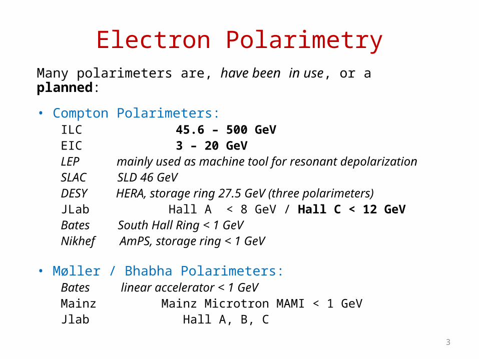
Electron PolarimetryMany polarimeters are, have been in use, or a planned:

• Compton Polarimeters: ILC 45.6 – 500 GeVEIC 3 – 20 GeVLEP mainly used as machine tool for resonant depolarizationSLAC SLD 46 GeV DESY HERA, storage ring 27.5 GeV (three polarimeters)JLab Hall A < 8 GeV / Hall C < 12 GeVBates South Hall Ring < 1 GeV Nikhef AmPS, storage ring < 1 GeV

• Møller / Bhabha Polarimeters:Bates linear accelerator < 1 GeVMainz Mainz Microtron MAMI < 1 GeVJlab Hall A, B, C

3

Laboratory Polarimeter Relative precision Dominant systematic uncertainty

JLab 5 MeV Mott ~1% Sherman function

Hall A Møller ~2-3% target polarization

Hall B Møller 1.6% (?) 2-3% (realistic ?)

target polarization, Levchuk effect

Hall C Møller 1.3% (best quoted)0.5% (possible ?)

target polarization, Levchuk effect, high current extrapolation

Hall A Compton 1% (@ > 3 GeV) detector acceptance + response

HERA LPol Compton 1.6% analyzing power

TPol Compton 3.1% focus correction + analyzing power

Cavity LPol Compton ? still unknown

MIT-Bates Mott ~3% Sherman function + detector response

Transmission >4% analyzing power

Compton ~4% analyzing power

SLAC Compton 0.5% analyzing power

Polarimeter Roundup

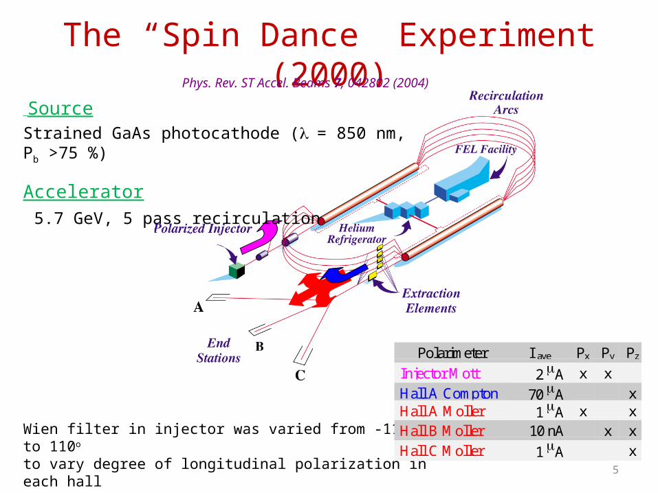
The “Spin Dance” Experiment (2000) SourceStrained GaAs photocathode (= 850 nm, Pb >75 %)

Accelerator 5.7 GeV, 5 pass recirculation

Wien filter in injector was varied from -110o to 110o

to vary degree of longitudinal polarization in each hall→ precise cross-comparison of JLab polarimeters

5

Polarimeter I ave Px Py Pz

Injector Mott 2 A x xHall A Compton 70 A xHall A Moller 1 A x xHall B Moller 10 nA x xHall C Moller 1 A x

Phys. Rev. ST Accel. Beams 7, 042802 (2004)

“Spin Dance” 2000 DataPmeas cos(Wien + )

Polarization ResultsResults shown include statistical errors only→ some amplification to account for non-sinusoidal behavior

Statistically significant disagreement

Systematics shown:

MottMøller C 1% ComptonMøller B 1.6%Møller A 3%

Even including systematic errors, discrepancy still significant

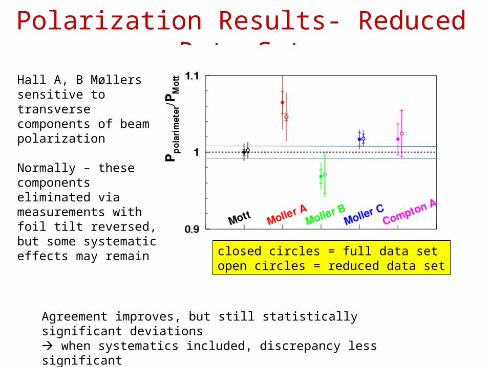
Polarization Results- Reduced Data SetHall A, B Møllers sensitive to transverse components of beam polarization

Normally – these components eliminated via measurements with foil tilt reversed, but some systematic effects may remain

closed circles = full data setopen circles = reduced data set

Agreement improves, but still statistically significant deviations when systematics included, discrepancy less significant

Lessons Learned• Providing/proving precision at 1% level challenging• Including polarization diagnostics and monitoring in beam lattice design is crucial • Measure polarization at (or close to) IP• Measure beam polarization continuously

– protects against drifts or systematic current-dependence to polarization

• Flip electron and laser polarization– fast enough to protect against drifts

• Multiple devices/techniques to measure polarization– cross-comparisons of individual polarimeters are crucial for testing systematics of each device– at least one polarimeter needs to measure absolute polarization, others might do relative measurements (fast and precise)– absolute measurement does not have to be fast

• New ideas? 9

532 nm HERA (27.5 GeV)

EIC (10 GeV)

Jlab

HERAEIC

-7/9

x 2maeE E E Compton edge:

Compton vs Møller Polarimetry

• Detect at 0°, e- < Ee

• Strong need <<1

• at Ee < 20 GeV

• Plaser ~100%• non-invasive measurement• syst. Error: 3 → 50 GeV (~1 → 0.5%) hard at < 1 GeV: (Jlab project: ~0.8%)• rad. corr. to Born < 0.1%

dA

dE/E E

• Detect e- at CM ~90°

• good systematics• beam energy independent• ferromagnetic target PT ~8%

• beam heating (Ie < 2-4 A), Levchuck eff.• invasive measurement• syst. error 2-3% typically 0.5% (1%?) at high magn. field• rad. corr. to Born < 0.3%

~ 090oCM

dA

d

eA EE

ILC

Polarized atomic hydrogen in a cold magnetic trap

• use ultra-cold traps (at 300 mK: Pe ~ 1-10-5, density ~ 3∙1015 cm-3 , stat. 1% in 10 min at 100 A)• expected depolarization for 100 A CEBAF < 10-4

• limitations: beam heating → “continuous” beam & complexity of target• advantages: expected accuracy < 0.5% & non-invasive, continuous, the same beam• Problem: very unlikely to work for high beam currents for EIC (due to gas and cell heating)• Jet Target: avoids these problems

– VEPP-3 100 mA, transverse– stat 20% in 8 minutes (5 ∙ 1011 e- /cm2 , 100% polarization)– What is electron polarization in a jet?

2bI

E. Chudakov et al., IEEE Trans. Nucl. Sci. 51, 1533 (2004)

• Jet Target: need to address these problems – Breit-Rabi measurement analyzes only part of jet → uniformity of jet has to be understood – large background from ions in the beam: most of them associated with jet (hard to

measure)– origin of background observed in Novosibirsk still unclear?– clarification of depolarization by beam RF needed → might be considerable

New Fiber Laser Technology (Hall C)

12

30 ps pulses at 499 MHz

- external to beamline vacuum → easy access- huge lumi boost when phase locked- excellent stability, low maintenance

Electron Beam LaserBeamJeff Martin (Winnipeg)

Gain switched

Compact, Off-The Shelf, Rack Mountable…

13

RF locked low-power1560 nm fiber diode

ErYb-doped fiber amplifier

Frequency doubler

Fiber Laser for Hall C Compton

14

• Seed laser at 1064 nm• Fiber amplifier (50 W output at 1064 nm)• Frequency doubling cavity• Result: 25 W, 532 nm, 30 ps pulses at 499 MHz• JLab Polarized source group is building laser (J. Grames)

• problems with amplification

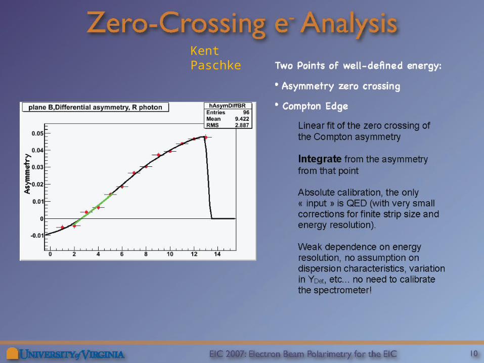
Dominant Challenge: determine Az

15

• Best tool to measure e- polarization → Compton e- (integrating mode)

• Challenge • accurate knowledge of ∫Bdl• must calibrate the electron detector• fit the asymmetry shape or use Compton Edge

Electron Polarimetry

9/14/2007 16W. Lorenzon PSTP 2007

Kent Paschke

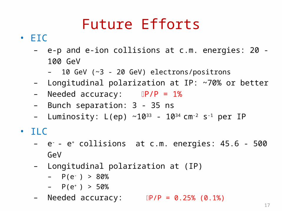
Future Efforts

17

• EIC– e-p and e-ion collisions at c.m. energies: 20 - 100 GeV

– 10 GeV (~3 - 20 GeV) electrons/positrons – Longitudinal polarization at IP: ~70% or better– Needed accuracy: P/P = 1% – Bunch separation: 3 - 35 ns– Luminosity: L(ep) ~1033 - 1034 cm-2 s-1 per IP

• ILC– e- - e+ collisions at c.m. energies: 45.6 - 500 GeV– Longitudinal polarization at (IP)

– P(e- ) > 80%– P(e+ ) > 50%

– Needed accuracy: P/P = 0.25% (0.1%) → new territory

EIC Compton Polarimeter

18

• No serious obstacles are foreseen to achieve 1% precision for electron beam polarimetry at the EIC (3-20 GeV)• JLAB at 12 GeV will be a natural testbed for future EIC e-/e+ Polarimeter tests

– evaluate new ideas/technologies for the EIC• There are issues that need attention (crossing frequency 3-35 ns; beam-beam effects at high currents; crab crossing effect on polarization)

ILC Polarimeters

19

• Three ways to measure polarization at the ILC• upstream Compton polarimeter• downstream Compton polarimeter• (e+e- →) W+W- production (has large cross section & very sensitive to polarization)

• Complication• polarization at IP = lumi-weighted polarization ≠ polarization at polarimeter• depolarization and spin transport effects estimated at 0.1%-0.4% levels!

• same level as required accuracy• keep errors in these effects small

• Need upstream, downstream & e+e- physics measurements• determine best values for each polarimeter separately (hide from each other)• compare and see whether they agree• final calibration with e+e- → W+W-

to e+e- IP: 1.8 km

upstream polarimeter

downstream polarimeter

~150 m behind IP

Goal: P/P ≈ 0.25% (0.1%)

Summary

20

• Electron beam polarization can be measured with high precision– no serious obstacles are foreseen to achieve 1% – imperative to include polarimetry in beam lattice design– use multiple devices/techniques to control systematics

• Big challenge to reach P/P = 0.25%– no fundamental show stoppers (but high beam energy needed)

• P/P = 0.1% enters new territory– goes beyond traditional polarimetry– use physics processes directly (W+W- production)

• Build on experience, but be open to new ideas– maybe use e-p elastic scattering at low energies (measures PePT) – …

• Extensive modeling necessary– AZ, depolarization, BMT, etc.– much work done, much work still ahead