precise transformation of classical networks to itrf...
TRANSCRIPT

Precise Transformation of Classical Networks to ITRF by CoPaG and Precise Vertical Reference
Surface Representation by DFHRS - General Concepts and Realisation of Data-
bases for GIS, GNSS and Navigation Applications1
1) Prof. Dr.-Ing. Reiner Jä ger and 2) Dipl.-Ing. (FH) Simone Kä lber
1) Fachhochschule Karlsruhe - University of Applied Sciences Studiengang Vermessung und Geomatik and
International Department and Programme Geomatics (MSc) Moltkestrasse 30, D-76133 Karlsruhe
Email: [email protected]. URL: www.dfhbf.de 2) Lamprechtstrasse 13, D-76227 Karlsruhe,
Email: [email protected]
1 Introduction As concerns the georeferencing of position data in modern data bases, the availability of GNSS (GPS/GLONASS/GALILEO) related code- and phase-measurement DGNSS-correction data, which are provided in different ways by different positioning services in and outside Europe leads to the replacement of the classical geodetic reference systems by GNSS-consistent ITRS-based reference systems. So the transformation of the old plan position data (N,E)class related to the classical reference systems to the ITRS/ETRS89 datum (N,E)ITRS becomes urgently necessary. A sophisticated and general solution of this transformation problem has to include a respective data base concept for the provision of the corresponding transformation parameters for GIS, GNSS and Navigation purposes. Further the capacity of a one-cm-positioning by GNSS services, such as e.g. SAPOS® and ascos® in Germany, is also appropriate for a GNSS related heighting. The GNSS-based determination of sea-level (orthometric, normal) heights H requires however the transformation of the ellipsoidal GNSS heights hITRS to the respective physically defined height reference surface (HRS). The first part of the contribution is dealing with the concept of a homogenizing precise and continuous transformation of plan positions (N,E)class to the ITRS/ETRS89 datum (N,E)ITRS. From the theoretical point of view a respective transformation can not renounce completely on height information. The presented so-called COPAG (COntinuously PAtched Geoferen-cing) concept however, has the advantage that the point height information is needed 1 Published as Jä ger R., Kä lber, S. (2006): Precise Transformation of Classical Networks to ITRF by CoPaG and Pre-
cise Vertical Reference Surface Representation by DFHRS - General Concepts and Realisation of Databases for GIS, GNSS and Navigation Applications. Proceedings to GeoSiberia 2006. Volume 1. S. 3-31. Novosibirsk, Russia. ISBN 5-87693-199-3.
only on a poor accuracy level. Further basic considerations and a respective problem solution for the plan datum transition are due to the occurrence and the mathematical treatment of so-called ‘weak-shapes. These are long-waved deflections of the network shape of the classical networks, reaching a range of several meters in the nation-wide scale, e.g. for the size of Germany. This requires the partition of the total network area into a set of different "patches”. The introduction of continuity conditions along the patch borders implies restrictions between the transformation parameters d of neighbouring patches. Because of its mathematical strictness and general validity the COPAG concept has (like the DFHRS approach below) a broad and far-reaching application profile in the context with the big amount of similar datum transition problems occurring world-wide in the upcoming GNSS-age. The realisation of a software system for the statistically controlled set up of a transformation parameter d data base for the transformation of positions (N,E)class to the ITRS datum (N,E)ITRS and vice verse is presented at different examples. The second part of the contribution is dedicated to the DFHRS (Digital-Finite-Element-Height-Reference-Surface) concept, which allows a GNSS height positioning (GPS/-GLONASS/GALILEO etc.) by a direct online conversion of ellipsoidal heights h into standard heights H referring to the height reference surface (HRS). The DFHRS model-led as a continuous HRS with parameters p in arbitrary large areas by bivariate polyno-mials over grid of Finite Element meshes (FEM). Geoid heights N, vertical deflections (ξ,η), gravity disturbances and anomalies ∆g and identical points (h, H) are to be used as observations in a least squares computation to derive the DFHRS-parameters p. Any number of geoid models may be introduced simultaneously and geoid models may be parted into different “patches” with individual datum-parameters in order to reduce the effect of existing medium- and long-waved systematic errors. So the resulting DFHRS parameters p, set up as a DRHRS data-base, provide a three-dimensional correction DFHRS(p|B,L,h) to transform by H=h-DFHRS(p|B,L,h) ellipsoidal GNSS heights h into standard heights H. The mathematical model of DFHRS computation and the software are pointed out. The authors present the results of DFHRS_DB computations for the GNSS online heighting in the cm-accuracy range for different countries and nations in and outside of Europe. Above the theoretical concepts the implementation and use of DFLBF_DB and DFHRS_DB in GNSS-equipment for real-time positioning in GNSS-services (e.g. SAPOS and Ascos) is shown, as well as the setting up the RTCM.3.0 transformation messages based on the above databases.
2 GNSS Plan Positioning – Data Bases to transform between ETRS89/ITRS and Classical Datum Systems
2.1 Continuous Patched Georeferencing (CoPaG) Concept This part of the contribution deals with the homogenisation, cm-accurate and neighbour-hood consistent transformation of plan coordinates between classical national reference-systems (N,E)Class and the unique ITRF/ETRS89-datum (N,E)ITRF. The so-called CoPaG (Continuously Patched Georeferencing) transformation concept [26] implies the improvement and homogenisation of the geometrical quality of existing
classical networks (such as e.g. the German DHDN network and datum, fig. 2.1; fig. 2.2) by the developed method of an ITRF/ETRS89 related georeferencing. So the qualification of the old position data for a future utilization and the continuation of existing databases are provided. Therefore also a high economic benefit as well as signals for further innovative developments in the GIS-, GNSS- and LBS-sector is set by the CoPaG concept of transforming the old classical data to the GNSS consistent ITRF/ETRS89 datum. The CoPaG concept is based on a strict three-dimensional similarity transformation between the two concerned reference-systems. The equations of this transformation are linearized under the realistic assumption of small rotation angles and the linearization point of the geographical coordinates (B,L,h)1. This leads to the resulting part for the plan component (B,L) of the three-dimensional similarity transformation in geographical coordinates (B,L,h) reading [8], [9], [26]:
( ) ( )
( ) ( ) [ ]
)b,b,a,a(BΔ mhM
eN)Bcos()Bsin(
ε0εhMhWaLcos ε
hMhWaLsin
whM
(B)cosvhM
(B)sinLsinuhM
(B)sinLcosB
)f,a,m,,ε,ε(u,v,w,εBB(d)BBvB
21211
2
zy1
x1
1111
zyx11112
∆+⋅
+⋅⋅⋅−
+⋅+⋅
++⋅
+⋅
++⋅
⋅−
+⋅
++⋅
+⋅−
+⋅
+⋅−
+=
∆∆∆∂+=∂+=+
( )( )
( )( ) [ ]
( ) ( )( )
( ) ( )( )
[ ] [ ] )b,b,a,a(Lm0 ε1
Bcosh)(N)h)e1(N(BsinLsin ε
Bcosh)(N)h)e1(N(BsinLcos
w0vBcosh)(N
LcosuBcosh)(N
LsinL
)f,a,m,,ε,ε(u,v,w,εLL(d)LLvL
2121z
1
2x
1
211
1
zyx11112
∆+∆⋅+⋅−
⋅
⋅++−⋅⋅⋅
+⋅
⋅
⋅++−⋅⋅⋅
+⋅+⋅
⋅+
+⋅
⋅+
−+=
∆∆∆∂+=∂+=+
(2.1a) (2.1b)
In the above formulas the following abbreviations were introduced:
)b,a(B)b,a(B)b,a,b,a(B 22112211 −=∆ ,
0)b,a(L)b,a(L)b,a,b,a(L 22112211 =−=∆ and
(2.1c,d)
Bcose1b
aN22'
2
⋅+⋅= ; 3
22'
2
Bcose1b
aM
⋅+⋅
= ; NaW = ; 2
222
abae −
= (2.1e,f,g, h)
As transformation parameters d (2.1a,b) three translations (u,v,w), three rotations (εx,εy,εz) and a scale difference ∆m between the two reference systems occur in the observation equations (2a,b). The corrections ∆B and ∆L (2.1c,d) are due to the known changes (∆a, ∆f) in the ellipsoid dimensions a and f at the transition from reference system 1 (e.g. DHDN in Germany) to reference system 2 (e.g. ETRS89). As the trans-

formation is concerning the plan component (B,L), and in general no heights for the re-spective identical points, nor for the points to be transformed (e.g. cadastral points, buildings etc.) are available in the different databases, the height component h – taken as third observation equation - is only needed for a small number of three dimensional identical points (e.g. points of a 1st order networks). The transformation equation for the height component h reads:
[ ] ( ) ( )[ ] ( )[ ]( ) ( ) ( )[ ] ( ) ( ) ( )[ ]
[ ] [ ] ),b,b,a,a(hmWah0
LcosBcosBsinNeLsinBcosBsinNe
wBsinvLsinBcosu)Lcos()Bcos(h
)f,a,m,,,,w,v,u(hh)d(hhvh
21211z
y12
x12
1111
zyx11112
∆+∆⋅⋅++ε⋅+
ε⋅⋅⋅⋅⋅+ε⋅⋅⋅⋅⋅−
+⋅+⋅⋅+⋅⋅+=
∆∆∆εεε∂+=∂+=+
(2.1h)
accordingly with )b,a(h)b,a(h)b,b,a,a(h 22112121 −=∆ . An advantage of the approach (2.1a-h) is that the ellipsoidal heights h1 (which are due to all classical network datum close to the standard heights H) are only needed with a subordinate accuracy. Due to the fact, that for the classical national datum systems the ellipsoid’s surface and the height reference surface were adapted to each other, the ellipsoidal height h1 in the co-efficients (2.1a) and (2.1b) can be replaced in different cases by the national standard heights H2. For the same, reason the height information h1 can in case of a classical system be taken from free available databases (e.g. the digital terrain model databases ETOPO5 or ETOPO30).
The formulas (2.1a-h) are based on a linearization, so that in case of large datum parameters d (e.g. for the translations u, v, w between two systems 1 and 2) a corres-ponding pre-transformation between system 1 and 2 with approximate parameters has to be performed before the application of (2.1a-h) [9].
2.2 CoPaG and DFLBF Data Bases (DB) for Germany Besides some solutions for different German states and city areas in Germany, two nationwide databases for Germany were computed with the CoPaG software, namely the “(3-5)_cm_CoPaG_DB Germany” (Fig. 2.2a) and the “(3-5)_cm_DFLBF_DB Germa-ny” (fig. 2.2b) [28].
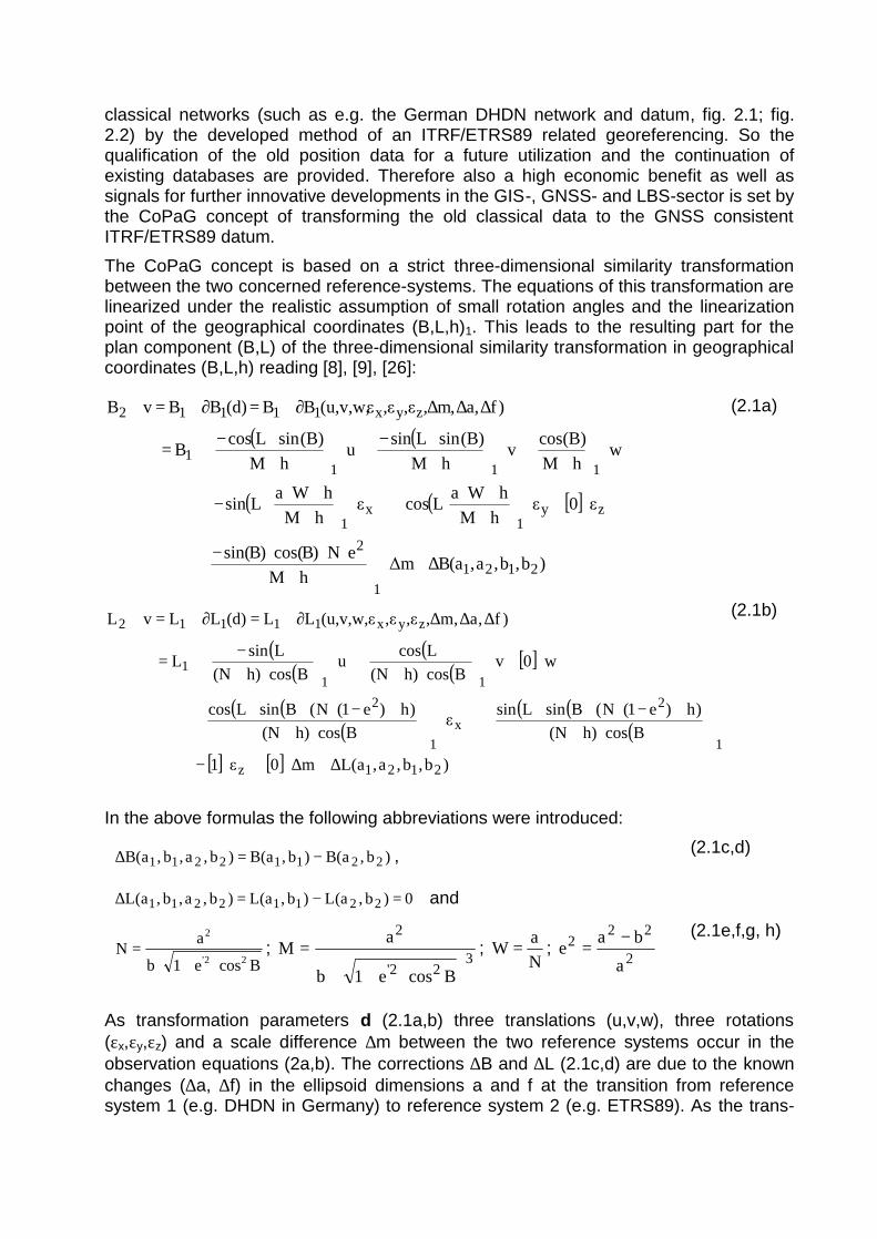
As the ETRS89 frame has one cm precision, e.g. all over Germany and the 1st Order ITRF/ETRS89 of other states all over the world, the residuals shown in fig. 2.1 left mean the deflection of the classical plan DHDN network coordinates x̂ =(B,L)1 from its true shape x~ . The residuals of the DHDN network of Germany West (fig. 2.1, left) reach the range of ± 2.5 m.
The shape and amount of the deflections x̂x~x −=∇ are to be explained by the theory of so-called “natural weak-shapes” [4], [5], [6], [15] and eventually a second part of so-called “stochastic weak-shapes” [10]. The “natural weak-shapes” of classical geodetic networks are related to the eigenvalue-problem
0 m]IC[ iix̂ =⋅⋅µ− . (2.2a)
of the covariance matrix x̂C of the adjusted network coordinates x̂ .
The eigenvalue problem (2.2a) is part of the theory and concepts of spectral analysis and optimization of geodetic networks [4], [7]. It is shown in [4], [5], [7], [15] and [9] that the spectral components i∇
iii m⋅µ=∇ . (2.2b)
are the key for the prediction (comparing e.g. the 1989 prediction results for Baden-Württemberg [6] with the real deflections for Baden-Württemberg presented 2000 in [9]) and theoretical understanding of deflections x̂∇ of large networks from their true shape x~ .
Fig. 2.1, left:
Residuals up to 2.5 m for the transformation of the German DHDN plan coordinates to ETRS89 with only one nationwide set of transformation parameters d.
Fig. 2.1, right:
Strict transformation with continuity conditions of the transformation parameters of the coordinates from German DHDN to ITRF (ETRS89) under partition in 177 patches. This leads to a drastic reduc-
tion of the residuals to less than 0.02 m in average.
In case of an occurring shape deflection x̂∇ - like shown for the plan German DHDN network in fig. 2.1, left - the spectral components i∇ (2.2b), which are carried by the eigenvectors im (2.2a) and scaled by the square roots of the corresponding eigenva-lues iµ (2.2a) give - in the descending order of the eigenvalue size iµ - the probability and amount of respective geometric deflection parts, which span up the total deflection shape x̂∇ (fig. 2.1,left). As large geodetic networks tend to have a number of high dominant eigenvalues, the maximum spectral components (2.2b) (especially the maximum component maxmaxmax m⋅µ=∇ ) point out the quasi systematic shape deflecttion x̂∇ . In case that the covariance matrix x̂C is regarded with respect to the assumed stochastical model of normal distributed observations, and the spectral

analysis is accordinly based on (2.2a,b), the essential main spectral components iii m⋅µ=∇ are called the “natural weak-shapes” of a geodetic network [4], [15].
Another type and an additional amount of weak-shape deflections x̂∇ - namely the so-called “stochastical weak shapes” stoch,istoch,istoch,i m⋅µ=∇ already mentioned above – occur due to neglections in the stochastic model of the observations of a geodetic net-work adjustment [5], or a non over-determined parameter-computation x̂ from a respec-tive observation set. The spectral components iii m⋅µ=∇ of the “stochastic weak- shapes” are then related to a general eigenvalue problem, which is regarded in [10].
Fig. 2.2a, b:
Left: DFLBF_DB for the transformation from ETRS89 to a classical plan reference system. Right: CoPaG_DB for the transformation from a classical plan reference
system to ETRS89. To manage the weak-shapes problem with respect to the plan transformation (2.1a,b), the transformation area has to be divided into so-called patches (fig. 2.1b) with individual datum parameter sets dj (accordingly the term CoPaG = Continuously Patched Georeferencing). In the example of applying the CoPaG concept to the plan German DHDN network, the average residual was reduced from 0.33 m (only one patch and datum set d for the whole area of Germany, fig. 2.1, left) to a range of less than 0.02 m by the division of the transformation area into 177 patches with individual datum parameters dj (fig. 2.1, right). To achieve a continuous and homogenising transformation, appropriate continuity con-ditions C(dj,dj+1) - in analogy to these of the DFHRS concept (3.6f) - along the borders of neighbouring patches j and (j+1) have to be set up as additional condition equations concerning neighbouring parameter sets dj and dj+1, in order to complete the COPAG adjustment approach (2.1a,b,h) [26]. The present CoPaG_DB and the DFLBF_DB (Digital Finite Element Plan Reference

System Transformation, in analogy to the term DFHBF, chap. 3) allow the strict and neighbourhood consistent transformation from/to the classical German reference-systems (e.g. DHDN in Western Germany presented in fig. 2.1 and RD83 in Eastern Germany) to/from ETRS89 with a reproduction quality of (3-5) cm.
2.3 CoPaG Software and CoPaG/DFLBF_DB Access Software The CoPaG approach (2.1a-h) was realized in the CoPaG-Software © Jä ger/Kä lber
Fig. 2.3:
View on the CoPaG Software at the example of the project “(1-2)cm DFLBF_BD and CoPaG_DB Rheinland-Pfalz”
The CoPaG software (fig. 2.3) allows the computation of transformation parameters dj on dividing the whole transformation area into an arbitrary number of irregular patches (fig. 2.1b, fig. 2.3).
Additionally continuity conditions C(dj,dj+1) have to be introduced to achieve the conti-nuity of the total set of parameters and the homogenisation of the transformed confi-guration. Fig. 2.3 shows a screen-shot of the CoPaG-Software at the example of the view on the CoPaG Software at the example of the project “(1-2)_cm DFLBF_DB and CoPaG_DB Rheinland-Pfalz”. Whereas in fig. 2.3 the mean meshsize is 15 km, the final meshsize for (1-2) cm databases was 7 km.

The quality control is – in addition to standards of statistical testing – performed by re-garding the quality measure of reproduction values. The two-dimensional test statistics and the so-called reproduction values are evaluated in the CoPaG concept and software in analogy to these of the quality control concept of DFHRS computation (see chapter 3.3.2). Besides this a so-called accuracy surface (Fig. 2.4) can be computed from the covariance-matrix in function of position. After finishing computation and quality control the parameter sets for all patches and also the residuals of the identical points are stored in a well-defined format in the so-called DFLBF_DB and CoPaG_DB files and can be used by any software providing a DFLBF/CoPaG Access.
Fig. 2.4:
Accuracy surface computed by the CoPaG-Software for Rheinland-Pfalz, Germany The direct access is realized by a DLL, which can be implemented into any GNSS or GIS software. Many GNSS and GIS companies meanwhile use a direct access. As concerns the alternative way of converting DFLBF_DB to gridfiles for a use in GNSS positioning in the so-called gridfactory philosophy and technology, e.g. within the Leica-Geosystem SKI_PRO software and the Trimble TSO software, it is referred to [28] and to the homepages of these companies respectively.
2.4 Outlook to the CoPaG Concept and CoPaG/DFLBF_DB The CoPaG_DB provide the direct transformation (no identical points) of the classical plan networks and related DB positions to the ETRS89 datum (fig. 2.2b), and the DFLBF_DB (fig. 2.2a) are used vice-verse for the direct transformation (no identical points) of ETRS89 related GNSS positions in SAPOS® - and ascos® GNSS positioning to the classical plan datum systems. The further development of the (3-5)_cm data bases, which is directed to the computa-

tion of a “1_cm_CoPaG_DB/DFLBF_DB for Germany” is merely a question of the num-ber and density of further identical points. This is to be concluded from successful test computations for the area of Rheinland-Pfalz, Germany, where a number of 2535 iden-tical points was used to evaluate the respective continuous transformation parameters sets ),...,...( nj1 dddd = enabling a mean reproduction quality of the coordinates of 1_cm.
The weak-shape problem (fig. 2.1, left) is of general nature, and it concerns all classical networks all over Europe and the whole world respectively. So the CoPaG concept can be applied generally to solve the related transformation problems and to evaluate precise and economic CoPaG_DB and DFLBF_DB worldwide.
3 GNSS-Heighting - Precise Vertical Height Reference Sur-face Representation by the Digital FEM Height Reference Surface Concept (DFHRS) and DFHRS Data Bases
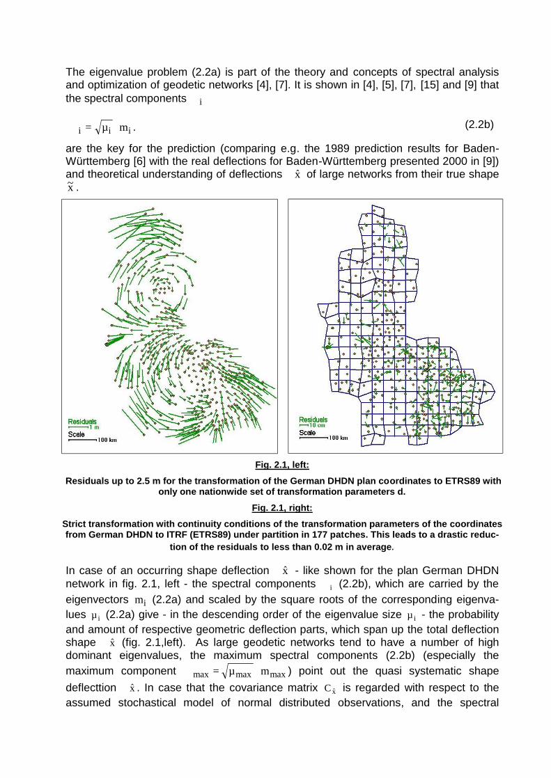
3.1 Motivation and Situation Standard heights H are referring to different types of height reference surfaces (HRS). The common root of all three relevant HRS-types is the idea, that the HRS should be that equipotential surface of the earth’s gravity field with a potential 0W , which coincides with the normal potential Uo and the mean sea-level surface H=0 (fig. 3.1, fig. 3.2)2 and continues it outside the oceans. The datum of a height system is fixed by at least one point with an assigned value 0W and H=0. The height HP of any point P on the earths surface (ES) is then defined as the curved distance between P and the respective HRS (fig. 3.1; fig. 3.2).
The two modern standard HRS-types are the geoid and the so called quasi-geoid. The geoid HRS type realizes exactly the equipotential surface concept. The related so-called orthometric heights g/)WW(H P0orth −= or g/CH Porth = respectively are found, by dividing the geopotential number CP (difference between W0 and the point P potential
PW ) by the mean gravity value g between P and the HRS. A disadvantage of a HRS type of a geoid and a related orthometric height system orthH is however due to the fact, that the density assumptions for the area of P are needed to evaluate g . The quasi-geoid HRS and the respective so-called normal heights γ= /CH Pnormal , as an alternative HRS and height system H, are found by dividing the geopotential number CP by the mean gravity value γ taken from the normal potential between P and the HRS. In
this case the modern standard for the normal potential and γ is related to the Global
Reference System 80 (GRS80). The value γ (B,h) is free from any density hypothesis. Therefore the decision for the new HRS and height type H for the European reference system EUREF was met for the quasi-geoid and normal height type H respectively (EUREF symposium, Ankara 1996, resolution No. 10, see [3]).
2 For the new Europe normal height system presently the Normaal Amsterdams Peils (NAP) [20]
The most precise way to determine the standard height of a point HP of the earth’s sur-face (ES) is still based on levelling, or better levelling and gravity measurements in higher order networks, meaning by the realization of the geopotential number PC as
∑ ∆⋅= iiP ngC .
The recent adjustment of the normal height H related European Vertical Network - as part of new European Vertical Reference System (EVRS) - was based on PC and is ready on the continental level [20]. The accuracy as e.g. predicted to be 5 cm on con-tinental level [5] is kept. The short-wave precision of the adjusted height differences H∆ of neighbouring points in the different European national networks of lower order is of course better and represented in the low sub-cm range [20].
ES
HRS
Ellipsoid
Fig. 3.1 (above):
Formula ideal (1a): earth surface (ES) at position P(B,L), ellipsoidal GPS/GNSS height h, standard height H and a two-di-mensional HRS model NG .
Fig. 3.2 (right):
In real world GNSS–positioning the exten-ded formulas (1b,c) and a three-dimensio-nal HRS model NG(B,L,h) however have to be taken into account.
The GNSS-based determination of standard heights H on any accuracy level however requires principally the transition of the ellipsoidal GNSS height h to the standard height H. So a GNSS-based determination of standard height H makes it necessary to subtract the height NG of the height reference surface (HRS) from the ellipsoidal GNSS height h (fig. 3.1; fig. 3.2). Therefore the HRS must be represented relative to the ellipsoid sur-face in terms of a two-dimensional HRS model NG(B,L). The old term “geoid” and “geoid height” for the HRS model and NG(B,L) (fig. 3.1) are getting properly replaced by “HRS” and “height of the HRS (fig. 3.2, DFHRS)”, which is more convenient with respect to the above mentioned different standard HRS and height types 3.
The classical gravity related geoid or quasi-geoid models NG(B,L), such as EGG97 [1], EGM96 [13] ) and the large number of local and regional geoid models are not fitted to
3 For historical reasons even some types more exist, such as e.g. the NN-type of HRS and the respective spheroidal normal heights (“NN-heights”) as precursor of the normal heights.

the HRS. This is for the reason, that the geometrical information of the identical points (h,H) is in general not taken into account art of a “geoid-computation” approach. A quasi-geoid for example is computed based on the Stokes formula as
∫∫σ
σ⋅ψ⋅∆γ⋅π
= d)S(g(B)4
a)L,B(N G . (3.1a)
In practice of course (3.1a) is submitted to the so-called remove restore technique and algorithm [1], whereas the global gravity reference EGM96 [13] is used as geopotential reference.
The precise geometric information for the HRS
L,BG )Hh()L,B(N −= (3.1b)
remains however unused as additional information in the state of the art of most gravity based geoid computation approaches. So the ideal formula
)L,B(NhH G−=
(3.2)
fig. 3.1 does not hold for the use of standard HRS in terms of “geoid-model” in GNSS-based heighting. In spite of a however sufficient HRS shape representation in the short wave range, HRS models represented by standard geoid models (3.1a) suffer from medium and long waved systematic shape deflections. The reasons are again a big amount of both types of “weak shapes” (chap. 2). Also for locally and short waved precise geoid models, e.g. the EGG97 [1], the “weak-shape” deflections reach a “meter range” over large areas e.g. for Europe (fig. 3.3). Of course the HRS represented by the standard height system H and h (3.1b) is also subjected to “weak-shapes” in H and h, but their amount is much smaller. For H they reach only in a “cm” range or a “few cm” range respectively in large areas [5], [15]. For Europe and the EVRS we have a range of 5 cm, see [5]. Consequently “levelled heights” H, which were evaluated from geopotential numbers (levelling and gravity) and the respective precise ellipsoidal heights h are representing by (3.1b) the precise and discrete control points for the long and short-wave domain of the HRS shape, while geoid-models of standard type NG(B,L) (3.1a) (fig. 3.3) can be used only as observations concerning the HRS shape in the local short wave domain.
An additional reason why (3.2) is not valid, is because of a scale difference ∆m occur-ring between the GPS/GNSS-heights h and the heights H of the standard height system ([2], [3], [18], [19]). One reason for scale inconsistency ∆m is, that most existing stan-dard height systems H were not evaluated by the GRS80 normal gravity field γ(B,h). Other proved sources for scale effects ∆m are occurring due to neglected (hidden) ob-servation correlations and related stochastic weak-shapes [5] and different systematic error types in levelling ([5], [10]). All these systematics tend to imply a scale error ∆m. So, all in all, the above formula ideal (3.2) has to be modified with respect to "real world conditions". In classical approaches ([2], [3]) and software packages like HEIDI2© Din-ter/Illner/Jä ger [3], which use explicitly geoid models NG(B,L) (3.1a), the relation bet-ween GNSS heights h and standards heights H reads:
Hm -) L)B,|NFEM(p )N( )L,B(N(hH regional
U
localG
HRS component" "3 sncontinuou⋅∆+∂+−=
44444444 344444444 21d (3.3a)

The formula (3.3a) represents the so-called “geoid-refinement approach” [3], [11], [14]. Here the geoid model heights NG(B,L) are used both as observations and as unknowns. So the geoid-model heights NG(B,L) become part of the HRS together with additional lo-cal datum parts )(N locald∂ , ]m,,,w,v,u[ Gyx
Tlocal ∆εε=d and an additional refinement
NFEM(p|B,L) component.
The refinement part NFEM(p|B,L), which is described theoretically in chap. 3.2, is based on the same mathematical concept of a surface representation as in the DFHRS concept. But it has a quite different meaning in the DFHRS concept than in the above classical geoid-refinement approach (3.3a). With respect to the determination of new points in the geoid-refinement approach (3.3a), the final HRS is to be considered as a compound of 3 components – the original and unimproved geoid-model NG(B,L), the local datum-parts )(N locald∂ and the refinement NFEM(p|B,L). The compound of a three component HRS would be a badly portable and heterogeneous concept for a data base in online GNSS heighting. Therefore the geoid refinement approach (3.3a) is in practice a post-processing solution. Above this, the effect of the local datum-parts )(N locald∂ of the geoid-model(s) (3.3a) introduced in the total area (3.3a), reading explicitly
m]N[
)]Lcos()Bcos()Bsin()B(Ne[ )]Lsin()Bcos()Bsin()B(Ne[
w)]B[sin( v)]Lsin()B[cos(u)]Bcos()Lcos([ )(N
GG
y2
x2
G
∆⋅−+
ε⋅⋅⋅⋅⋅−+ε⋅⋅⋅⋅⋅+
⋅+⋅⋅+⋅⋅=∂ d
(3.3b)
is not controlled with respect to the continuity of the three-component HRS model at the borders of the local areas. These are some decisive disadvantages of the “geoid refine-ment” approach (3.3a). The datum part (3.3b), which is also used in (3.6a), is - except the simplified scale part m]N[ GG ∆⋅− of the geoid model NG - identical with (2.1h).
In the DFHRS approach [11], [16], [17], [18], [21], [22], [23] and the computation of DFHRS_DB [14], [26], [27], [28] for GNSS-based heighting, which are further treated as main subject of chap. 3, however the role of the former three-component HRS model (3.3a) is completely taken over by the one-component HRS model of a Digital Finite Element Height Reference Surface (DFHRS).
In DFHRS modelling the HRS is described continuously by the surface NFEM(p|B,L).
The two-dimensional Finite Element Model (FEM) NFEM(p|B,L) (3.5a) of the HRS takes over the role of the HRS (fig. 3.1; fig. 3.2), and is represented in a continuous way by mesh-wise sets of polynomial parameters p (3.5b). So we have for the DFHRS concept the following basic relation between the ellipsoidal GNSS height h and the standard height H (fig. 3.1; fig. 3.2):
Hm - HRS component" -one" Continuous
L)B,|NFEM(hH regional ⋅∆−=44 344 21
p (3.4a)
In this way the continuous Finite Element Model NFEM(p|B,L) of the HRS is a two-dimensional function of the plan position (B,L), and is accordingly called the “geoid-part” of the so-called three-dimensional DFHRS correction. The part ∆m⋅h is accordingly called the “scale part” of the DFHRS correction.

So three-dimensional DFHRS correction DFHRS(B,L,h) (fig. 3.2), which has to be subtracted from the GNSS height h in order to receive the standard height H, reads in total:
)Hm)L,B|(NFEM(h )h,L,B|m,DFHRS( -h H ⋅∆−−=∆= pp (3.4b)
The respective DFHRS data bases (DB) contain - as essential parts for HRS representation and the scale parametrisation - the “DFHRS_DB parameters” p and m∆ .
Fig. 3.3.:
Long-waved deflections, to be declared as natural and stochastic “weak-shapes” (chap.1), in the (dm – meter) range of the EGG97, which has above these long-waved distortions a
cm-accuracy concerning the local shape quality (published in different EUREF series, [20])
3.2 FEM representation of a Height Reference Surface (DFHRS) The finite element representation NFEM(p|x,y) is carried by the base functions of biva-riate polynomials of degree n, which are set up in regular or irregular meshes. If we describe with pi the polynomial coefficients (a00, a10, a01, a20, a11, a02,...)i of the i-th mesh, we have for the height NFEM(pi|x,y) of the HRS over the ellipsoid (fig. 3.1; fig. 3.2) in the i-th mesh:
. ²,...)y,xy²,x,y,x,1())L,B(y),L,B(x( and,....)a,a,a(
withm;1,i ; ))L,B(y),L,B(x()y,x|(NFEMi
011000i
ii
==
=⋅=
fp
pfp
(3.5a)
(3.5b), (3.5c)
The vector f means the so called Vandermond vector and contains the different powers of the coordinates (x,y) according to the polynomial degree n. The total parameter vector p consists of the coefficient sets pi=(aj,k)i, (j=0,n; k=0,n) of all m meshes. The plan position in (3.5a,c) is due to metric ellipsoidal coordinates (y(B,L)=“East” and x(B,L) =“North”) introduced e.g. as Mercator or Lambert coordinates, which are in any case functions of the geographical coordinates (B,L). To imply a continuous surface NFEM(p|x,y), one set of continuity conditions of different type C0,1,2 has to be set up for the computation of NFEM(p|x,y) for each couple of neigh-bouring meshes (fig. 3.4). The continuity type C0 implies the same functional values, the continuity type C1 implies the same tangential planes and the continuity type C2 the same curvature along common mesh borders of the DFHRS as represented by NFEM(p|x,y) (3.5a). The continuity conditions occur as additional observation equations C(p)=0 to be added to the parametrization of NFEM(p|x,y). The condition equations C(p)=0 are related to the polynomial sets of the coefficients (ajk)m and (ajk)n of each couple of neighbouring meshes m and n. To force e.g. C0-continuity, the difference ∆Nm,n in the geoid height NG of any point S at the common border SA–SE of two meshes m and n (see fig. 3.4; fig. 3.8) has to become zero. So the basic condition equation for a polynomial representation of nth degree reads [22]:
. 0 k))SExSAx(tSAx(j))SEySAy( tSAy(n0j
j n0k )m,jkan,jka( n,mN ≡⋅+⋅−⋅+⋅∑ = ∑ −
= −=∆ (3.5d)
With )x,y,x,y( SESESASA we introduce the plan metric coordinates of the nodal points SA and SE of a mesh borderline. Equation (3.5d) represents a polynomial of n-th degree parametrized in the border line parameter t with ]1,0[t ∈ . The subset of (n+1) C0-con-tinuity condition equations C(p)=0 for the border between mesh m and n results in case of C0-continuity from (3.5d) by setting all (n+1) coefficients related to t to zero ([22]). The mesh size and mesh shape for the computation of the NFEM(p|x,y) - representing the so called HRS or "geoid” part (3.3a) of the DFHRS correction and DB content - may be chosen with an arbitrary shape. The best approximation of a HRS by NFEM(p|x,y) results of course by introducing small meshes, e.g. in a range of 5 km to keep a 5 mm range for any HRS shape approximation by a polynomial degree up to n=3. A special advantage and characteristic of the NFEM(p|x(B,L), y(B,L)) representation consists in the fact, that the nodal points of the FEM grid are totally independent of the location of the geodetic observations and the geoid data points. In principle any type of HRS and height related observation data can be used for the determination of the para-meter vector p of NFEM(p|x,y), namely height observations (h,H,∆H,∆h), the geoid-model heights NG(B,L), deflections of the vertical (ξ,η) and gravity anomalies ∆g (see chap. 3.3).

3.3 Digital FEM Height Reference Surface (DFHRS) Approach and Computation
3.3.1 Mathematical Adjustment Model The mathematical model of the so-called DFHRS data base production step reads in the system of observation equations (functional model) and the corresponding stochastic models of a least squares adjustment as follows: Functional Model Observation Types and
Stochastic Models
pfp
pf
⋅=
⋅+∆⋅+=+
))L,B(y),L,B(x(: y)x,|NFEM( with
, )y,x( mh Hvh
Uncorrelated observations of ellipsoidal heights h Covariance
matrix )(diag 2hh i
σ=C .
(3.6a)
)(N)y,x(v)L,B(N jG
jG dpf ∂+⋅=+ Correlated geoid height observa-
tions. With a given real covariance matrix CN,G or a CN,G evaluated from an artificial covariance func-tion.
(3.6b)
)(L))Bcos()B(N/(v
)(B)B(M/v
,L
,B
ηξ
ηξ
∂+⋅⋅−=+η
∂+⋅−=+ξ
dpf
dpf
Observations of vertical deflections (η,ξ). Pairwise correlated or uncor-related among each other in case of astronomical observations. Corre-lated in case of being taken from a gravity potential model.
(3.6c)
(3.6d)
HvH =+ Uncorrelated standard height H observations with covariance matrix
)(diag 2HH i
σ=C .
(3.6e)
)(CvC p=+ Continuity condition equations (3.5d) introduced as uncorrelated so-called pseudo observations with accordingly small variances and high weights.
(3.6f)
With fB and fL we introduce the partial derivatives of the Vandermonds' vector f(x(B,L),y(B,L)) (3.6c) with respect to the geographical coordinates B and L. M(B) and N(B) mean the radius of meridian and normal curvature at a position P(B,L) respective-ly. The continuity of the resulting HRS NFEM(p|x,y)=f(x,y)⋅p is automatically provided by the continuity equations C(p) (3.6f). A number of identical points (h, H) (3.1b) are introduced by the observation equations (3.6a) and (3.6e). In the practice of DFHRS data base evaluation, also one or a number of several geoid models NG(B,L)j are used as additional observations to produce DFHRS_DB in the least squares estimation (3.6a-k). To reduce the effect of medium or long waved systematic shape deflections, namely the natural and stochastic “weak-shapes” (chap. 2) of geoid models NG (3.6b) (fig. 3.3), the geoid model heights observations NG (3.6b) are parted to into a number of so-called “geoid-patches”
jG )L,B(N (3.6b) (see fig. 3.8). Each patch is set up, with individual datum-parameters dj,
which are introduced by the datum part ∂NG(dj) (3.3b) into (3.6b). It is of course also possible to introduce by NG(B,L)j - and a respective parametrization ∂NG(dj) - (3.6b)
several patched or unpatched geoid models in the same area, and of course also geoid models of a different type than the classical ones (3.1a) may be used.
With the classical relations ξ = - ∂N/∂sB and η= - ∂N/∂sL between vertical deflections and the 1st derivatives of the HRS in northern and eastern direction and the NFEM- polyno-mial representation as a product (see (3.5a-c) and (3.6a)) of Vandermond’s vector f and the polynomial parameters p we get :
ξ = - ∂N/∂sB = - ∂NFEM/∂B ·∂B/∂sB = - f(x(B,L),y(B,L))B ⋅ p · ∂B/∂sB, (3-6g)
η = - ∂N/∂sL = - ∂NFEM/∂L ·∂L/∂sL = - f(x(B,L),y(B,L))L ⋅ p ⋅ ∂L/∂sL . (3-6h)
For ∂B/∂sB and ∂L/∂sL we have the classical relations ∂B/∂sB=M(B) and ∂L/∂sL=N⋅cos(B). With ∂B(dξ,η) and ∂L(dξ,η) we describe the datum parts of the type deflections of the ver-tical ξ = )B( astr −ϕ and η = Bcos)L( astr ⋅−λ respectively. According to these definitions we receive the datum-parts ∂B(dξ,η) and ∂L(d ∂B(dξ,η) by introducing (2.1a) and (2.1b). So it holds that ∂B(dξ,η) )d(B1−∂≡ (2.1a) and ∂L(dξ,η) Bcos)d(L1 ⋅−∂≡ .
Using the vertical deflections (ξ, η), which were derived from the same geopotential model as the geoid-model NG, the datum parameter d are also expected to be the same, and it holds d(3.6b) = dξ,η(3.6c)=dξ,η(3.6d). Otherwise, e.g. for sets of astronomi-cally observed vertical deflections, different groups of datum parameters d have to be introduced.
Observations from classical geoid models NG (3.6b) are to be introduced instead of the original gravity observations ∆g, which had been introduced for the computation of NG. In this case the correlated geoid models observations NG (3.6b) and original gravity ob-servations ∆g lead to identical results for the HRS by the parameters p ([22], [23]). So the use of observation type NG (3.6b) allows a more elegant and easier data treatment than by the use of the original gravity anomalies ∆g (3.6i). Consequently observation equations for gravity observations ∆g need to be set up in the DFHRS approach (3.6a-k), only if additional gravity observations ∆g occur, which have not yet been used for the former computation of a geoid model NG (3.6b).
Functional Model Observation Types and Stochastic Model
y)x,|NFEM(
)y,x(v d)S(g(B)4
a
p
pf
=
⋅=+σ⋅ψ⋅∆γ⋅π ∫∫
σ Vector of reduced gravity anomalies ∆g in-troduced with covariance matrix Cg into Stokes formula. The gravity anomalies ∆g in this way determine the DFHRS with parameters p at position (x(B,L),y(B,L)) .
(3.6i)
The integration of gravity observations g is done by the functional model (3.6j). The gra-vity observation g is represented in the local astronomical vertical system by the vector
TLAV ]g,0,0[ −=g . It is reduced due to vertical defelctions (“topography”) and then rotated to the system referring to the pole ),( 00 λϕ of a local spherical cap harmonics (SCH) repre-sentation ([34] ,[35]).
Functional Model Observation Types and Stochastic Model

)','|S,C(v nmnm υλ=+ gg g
Gravity vector taken from original gravity measurement vectors TLAV ]g,0,0[ −=g in the local astronomical ver-tical system (LAV), reduced for vertical deflections and transformed to the SCH-system referring to ),( 00 λϕ .
(3.6j)
With )','( υλ we introduce the local azimuth-coordinates referring to the SCH-pole ),( 00 λϕ . Besides (3.6j) existing geopotential models, e.g. EGM96, are to be introduced as direct observations for the regional SCH-parametrization nmnm S,C . The advantage of a regional SCH-parametrization - compared to the standard of a global spherical representation – is, that for a sub-cm resolution a SCH-order of n=m=25 is sufficient for an area-size of (100 km x 100 km) compared to n=m=7000 for the a global harmonics parametrization. So the number of unknowns is to be reduced essentially. The SCH-parameters nmnm S,C (3.6j) are regarded as auxiliary unknowns. By the condition equation (3.6k) these are related to the NFEM parameters p of the DFHRS-approach, see [34].
Functional Model Observation Types and Stochastic Model
( ) ( )∑∑=
∞
=
+∆
υ⋅λδ+λδ
γ
=+
n
0mnmnmnm
2n
1nN
'cosP'msinS'mcosCra
aGM
v0
- pf ⋅
Condition equations “HRS from N(SCH) = NFEM(p)” as uncorre-lated pseudo observa-tions with small variances and es and high weights.
(3.6k)
The approach (3.6a-k) means all in all a new method and standard (fig. 4.1), both for the over-determined boundary value problem (geoid-determination), and for the solution of a direct and online GPS/DGNSS-heighting (fig. 4.1) by the use of DFHRS databases and the respective DFHRS correction (3.4b).
3.3.2 DFHRS Software and Quality Control in DFHRS_DB Computation The DFHRS approach (3.6a-k) has been realized in the software DFHBF© Jä -ger/Schneid/Schwarzer. There the mathematical model of the DFHRS approach (6a-i) is embedded in the quality control standards of a priori and a posteriori variance related tests (data snooping) and variance component estimations.
The covariance matrix of the resulting DFHRS_DB parameters (p, ∆ m) can be used to compute and visualize the precision of the HRS and/or DFHRS correction surface (fig. 3.5).
An additional and valuable way to prove the “external accuracy” of the DFHRS_DB is to compute a so-called “reproduction quality” and point-wise reproduction values [16], [17], [18].

Fig. 3.4:
Screen shot of the DFHRS software. Continuity of the resulting HRS along the mesh borders of two general meshes m and n is provided by the continuity equations (3.6f). Identical
points (3.1b) in green.
The “reproduction quality” and a number of n resulting “reproduction values iH∇ “ - all over the DFHRS area - are simply defined by the values of differences:
))H without:(DFHRS(H - H H iiiii ==∇ , with
))h,L,B(|m,(DFHRSh)DFHRS(H iiiii ∆−= p (3.7a)
For this quality proof no explicit “control measurements” are needed. We just have to compute successively the "DFHRS-height" H(B,L,h,DFHRS)i of each of the n identical standard height points Hi from hi, when using the individual data base DFHRSi, where Hi was excluded from the respective DFHRS_DB production (3.6a-k) (“new point”), which was then evaluated with the rest of the (n-1) points.
The “reproduction values” iH∇ are much more objective and informative than the pure least squares residuals vi (3.6e). The reproduction values iH∇ are to be computed in the unique DFHRS production step (3.6a-k) of the DFHRS adjustment. The respective formula reads:
. rv
HiH
iHi −=∇ (3.7b)
With iHv and ir we describe the correction and the redundancy part of Hi in equation
(3.6e).
The above reproduction values (3.7a, b) are however only directly interpretable as a quality measure, if they are applied to the part of the high accurate identical points (h,H).
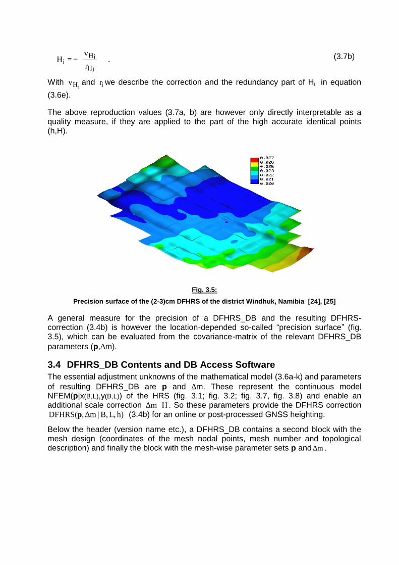
Fig. 3.5:
Precision surface of the (2-3)cm DFHRS of the district Windhuk, Namibia [24], [25]
A general measure for the precision of a DFHRS_DB and the resulting DFHRS-correction (3.4b) is however the location-depended so-called “precision surface” (fig. 3.5), which can be evaluated from the covariance-matrix of the relevant DFHRS_DB parameters (p,∆m).
3.4 DFHRS_DB Contents and DB Access Software The essential adjustment unknowns of the mathematical model (3.6a-k) and parameters of resulting DFHRS_DB are p and ∆m. These represent the continuous model NFEM(p|x(B,L),y(B,L)) of the HRS (fig. 3.1; fig. 3.2; fig. 3.7, fig. 3.8) and enable an additional scale correction Hm ⋅∆ . So these parameters provide the DFHRS correction
h)L,B,|m,DFHRS( ∆p (3.4b) for an online or post-processed GNSS heighting.
Below the header (version name etc.), a DFHRS_DB contains a second block with the mesh design (coordinates of the mesh nodal points, mesh number and topological description) and finally the block with the mesh-wise parameter sets p and m∆ .
3.5 Evaluation of the European HRS as part of the European Vertical Reference System (EVRS)
3.5.1 Preliminary Notes An essential and very precious characteristic of the embedded FEM principle is, that any DFHRS_DB and its reproduction quality (3.7a,b) respectively, which was achieved by using the DFHRS approach (3.6a-k) in a small area, is to be achieved - without loss of accuracy - in a corresponding large area scene, only provided that the density of the identical points (H,h) and the quality of the geoid information NG are kept!
So it is clear, that a 1st class of
§ “<_1cm_DFHRS_DB” defined by a mean reproduction value cm 1 H i ≤∇ (3.7a,b) over all precise and not rejec-ted identical points (3.1b), (3.6a), (3.6e) and a respective “precision surface” (fig. 3.5) better than 1 cm - is to be computed by the DFHRS approach and the DFHRS software with a mesh size of 5 km, a density of about 50 identical points (H, h) per (100 km x 100 km) area, and a (30 - 40) km geoid-model “patch” size. Above these design parameters, the total size of the area does not play any role, so that this quality can be produced also e.g. in the European scale! Different “<1_cm_DFHBF_DB”, which represent the present “high end” quality type, have already been computed [18]. They are available as official geo-data products of different German state land service departments (Saarland, Baden-Württemberg, Hessen, Rheinland-Pfalz, Bayern and Hannover district) [19], and they are used in SAPOS® and ascos® GNSS services in these parts of Germany (fig. 3.6). Above these German countries presented in fig. 3.6, another “1_cm_DFHRS_DB” was computed for the region of Tallinn, Estonia, and a (2-3)_cm DFHRS_BD was computed for the district of Windhuk, Namibia [24], [25] based on the EGM96 [13], (fig. 3.5).
The 2nd quality class of a
§ “<_3cm_DFHRS_DB” is defined by mean reproduction value cm 3 Hi ≤∇ (3.7a,b) over all precise and not rejected identical points, and a respective “precision surface” (fig. 3.5) better than 3 cm. A “<_3cm_DFHRS_DB Germany” was evaluated by a density of less than 10 identical points (H, h) per (100 km x 100 km) area, a mesh size of 10 km, and a polynomial degree n=3.

Fig. 3.6:
Existing “1_cm_DFHRS_DB” in the German countries Saarland, Rheinland-Pfalz, Baden-Würt-temberg, Hessen, Bavaria and Hannover district (orange) and those, which are planned (green).
The number of patches was 102 and the patch size was about 50 km. Fig. 3.7 above shows the isolines of the corresponding HRS (fig. 3.1; fig. 3.2) NFEM(p|B,L) of the “<_3_cm_DFHRS_DB Germany”. It is already related to the new European normal height system. For the former West Germany another “<_3_cm_DFHRS_DB Germany” related to the classical NN-height system was computed additionally. The “<_3_cm DFHRS_DB” is applied for GNSS online and post-processing heighting by the users of SAPOS® and ascos® DGNSS services [26], [27], [28]. Above the “3_cm_DFHBRS_DB Germany” a “5_cm DFHRS_DB Valencia” (fig. 3.8) was computed for the district of Valencia, Spain [30]. A closed and continuous solution of a “(1-3)_cm_DFHRS_DB Baltic States” (fig. 3.8) was computed for the Baltic States Estonia, Latvia and Lithuania in the frame of a cooperation with the State Land Service of Latvia, Riga [29], and a “(2-3)_cm DFHRS_BD Windhuk” was computed for the district of Windhuk, Namibia [24], [25] based on the EGM96 [13], (fig. 3.5).
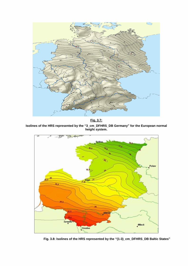
Fig. 3.7:
Isolines of the HRS represented by the “3_cm_DFHRS_DB Germany” for the European normal height system.
Fig. 3.8: Isolines of the HRS represented by the “(1-3)_cm_DFHRS_DB Baltic States”
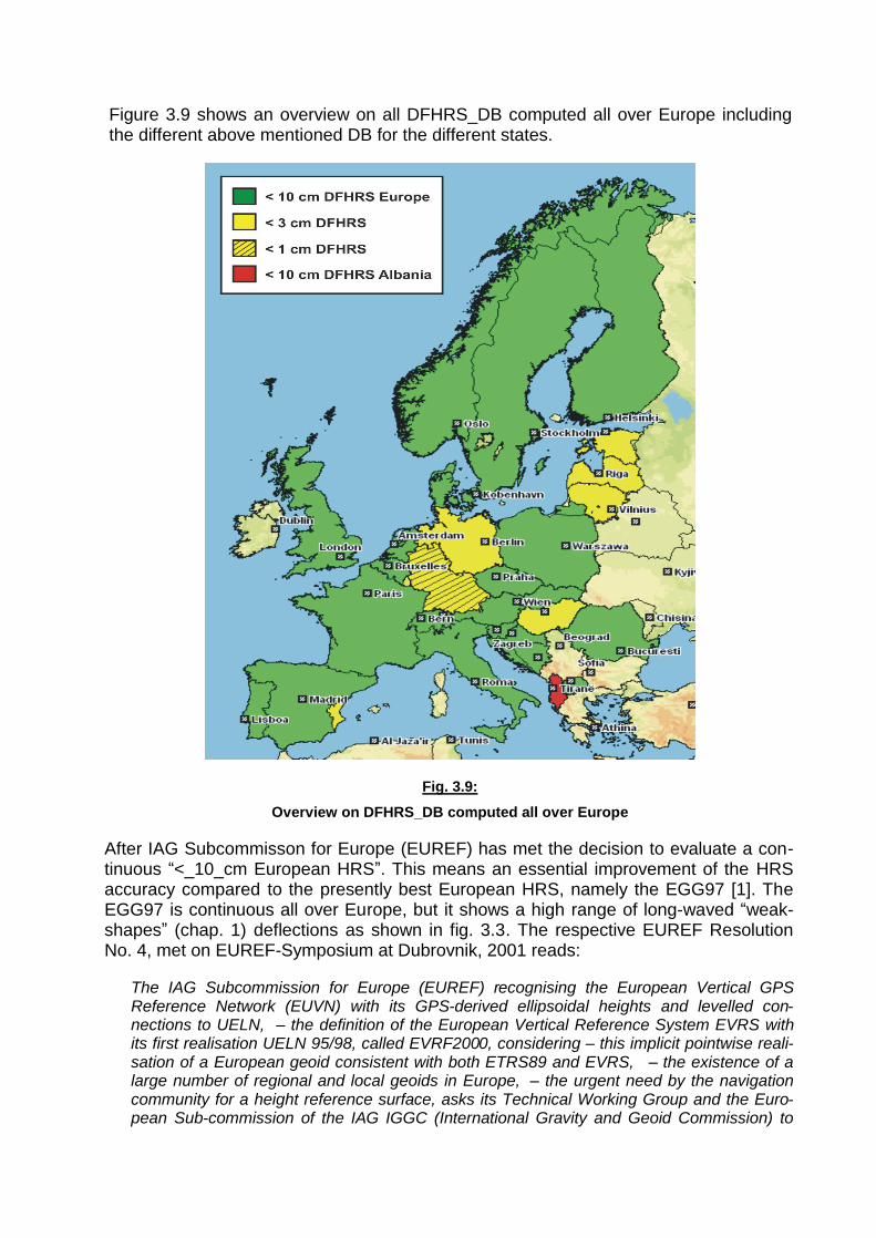
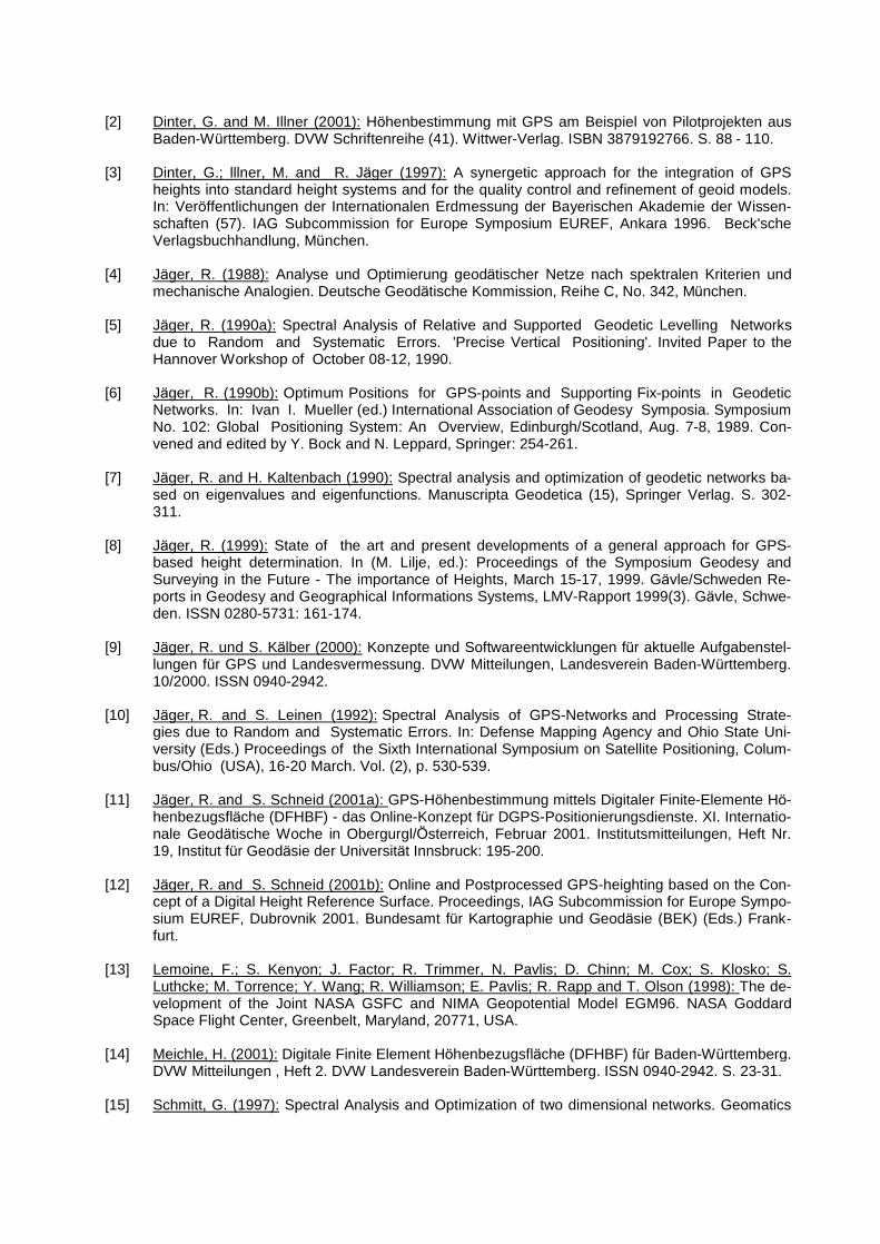
Figure 3.9 shows an overview on all DFHRS_DB computed all over Europe including the different above mentioned DB for the different states.
Fig. 3.9:
Overview on DFHRS_DB computed all over Europe
After IAG Subcommisson for Europe (EUREF) has met the decision to evaluate a con-tinuous “<_10_cm European HRS”. This means an essential improvement of the HRS accuracy compared to the presently best European HRS, namely the EGG97 [1]. The EGG97 is continuous all over Europe, but it shows a high range of long-waved “weak-shapes” (chap. 1) deflections as shown in fig. 3.3. The respective EUREF Resolution No. 4, met on EUREF-Symposium at Dubrovnik, 2001 reads:
The IAG Subcommission for Europe (EUREF) recognising the European Vertical GPS Reference Network (EUVN) with its GPS-derived ellipsoidal heights and levelled con-nections to UELN, – the definition of the European Vertical Reference System EVRS with its first realisation UELN 95/98, called EVRF2000, considering – this implicit pointwise reali-sation of a European geoid consistent with both ETRS89 and EVRS, – the existence of a large number of regional and local geoids in Europe, – the urgent need by the navigation community for a height reference surface, asks its Technical Working Group and the Euro-pean Sub-commission of the IAG IGGC (International Gravity and Geoid Commission) to

take all necessary steps to generate a European geoid model of decimetre accuracy con-sistent with ETRS89 and EVRS.
The required
§ “<_1_dm DFHRS_DB Europe” (fig. 3.9, green) was computed in a short-term project at the Karlsruhe University of Applied Sciences by using the DFHRS concept (3.6a-k) and the DFHRS software [31].
Besides the computation of DFHRS_DB for Europe and the European states [32] a DFHRS_DB for for Florida, USA was computed in the frame of a master-thesis at the HS Karlsruhe.
For further information it is referred to the DFHRS homepage www.dfhbf.de [27].
Fig. 3.10 (a, b):
USA map (right) and meshing (left) for the < 5 cm DHHRS_DB Florida, which was computed in the frame of a master-thesis at the HS Karlsruhe.
4 Standardisation of DFLBF/CoPaG and DFHRS Data Bases For the implementation of a DFLBF/CoPaG and a DFRHS_DB access respectively into existing software packages (fig. 4.1, 4.2), DFLBF/COPAG and DFHRS_DB access software have been realized as DLL (Dynamics Link Library) [27], [28].

Fig. 4.2:
DFLBF/CoPaG and DFHRS access realized in Trimble Survey Manager Software (left) and in the Leica Field Software Package (right).
Fig. 4.3:
DFLBF/CoPaG and DFHRS access realized in the GNSS controller-software TopSURV of TOPCON company (www.topcon.de).
The growing acceptance and the different implementations of the DFLBF/COPAG and DFHRS database standard into different GNSS equipments and software packages of the GNSS industry are shown in fig. 4.2 and fig. 4.3. Besides the GNSS domain, the DB and DB access software is used and implemented into different GIS software packages (fig. 4.1.b). For details it is referred to [27] and [28].
Finally it is mentioned, that the DFHRS_DB and DFLBF_DB can be converted consistently and directly into the new RTCM 3.0 transformation messages 1022-1028 [33].
5 References [1] Denker, H. and W. Torge (1997): The European Gravimetric Quasigeoid EGG97 – An IAG sup-
ported continental enterprise. In: Geodesy on the Move – Gravity Geoid, Geodynamics, and Ant-artica. R. Forsberg, M. Feissel, R. Dietrich (eds.). IAG Symposium Proceedings Vol. 119, Sprin-ger, Berlin Heidelberg New York: 249-254.
[2] Dinter, G. and M. Illner (2001): Hö henbestimmung mit GPS am Beispiel von Pilotprojekten aus Baden-Württemberg. DVW Schriftenreihe (41). Wittwer-Verlag. ISBN 3879192766. S. 88 - 110.
[3] Dinter, G.; lllner, M. and R. Jäger (1997): A synergetic approach for the integration of GPS heights into standard height systems and for the quality control and refinement of geoid models. In: Verö ffentlichungen der Internationalen Erdmessung der Bayerischen Akademie der Wissen-schaften (57). IAG Subcommission for Europe Symposium EUREF, Ankara 1996. Beck'sche Verlagsbuchhandlung, München.
[4] Jäger, R. (1988): Analyse und Optimierung geodä tischer Netze nach spektralen Kriterien und mechanische Analogien. Deutsche Geodä tische Kommission, Reihe C, No. 342, München.
[5] Jäger, R. (1990a): Spectral Analysis of Relative and Supported Geodetic Levelling Networks due to Random and Systematic Errors. 'Precise Vertical Positioning'. Invited Paper to the Hannover Workshop of October 08-12, 1990.
[6] Jäger, R. (1990b): Optimum Positions for GPS-points and Supporting Fix-points in Geodetic Networks. In: Ivan I. Mueller (ed.) International Association of Geodesy Symposia. Symposium No. 102: Global Positioning System: An Overview, Edinburgh/Scotland, Aug. 7-8, 1989. Con-vened and edited by Y. Bock and N. Leppard, Springer: 254-261.
[7] Jäger, R. and H. Kaltenbach (1990): Spectral analysis and optimization of geodetic networks ba-sed on eigenvalues and eigenfunctions. Manuscripta Geodetica (15), Springer Verlag. S. 302-311.
[8] Jäger, R. (1999): State of the art and present developments of a general approach for GPS-based height determination. In (M. Lilje, ed.): Proceedings of the Symposium Geodesy and Surveying in the Future - The importance of Heights, March 15-17, 1999. Gä vle/Schweden Re-ports in Geodesy and Geographical Informations Systems, LMV-Rapport 1999(3). Gä vle, Schwe-den. ISSN 0280-5731: 161-174.
[9] Jäger, R. und S. Kä lber (2000): Konzepte und Softwareentwicklungen für aktuelle Aufgabenstel-lungen für GPS und Landesvermessung. DVW Mitteilungen, Landesverein Baden-Württemberg. 10/2000. ISSN 0940-2942.
[10] Jäger, R. and S. Leinen (1992): Spectral Analysis of GPS-Networks and Processing Strate-gies due to Random and Systematic Errors. In: Defense Mapping Agency and Ohio State Uni-versity (Eds.) Proceedings of the Sixth International Symposium on Satellite Positioning, Colum-bus/Ohio (USA), 16-20 March. Vol. (2), p. 530-539.
[11] Jäger, R. and S. Schneid (2001a): GPS-Hö henbestimmung mittels Digitaler Finite-Elemente Hö -henbezugsflä che (DFHBF) - das Online-Konzept für DGPS-Positionierungsdienste. XI. Internatio-nale Geodä tische Woche in Obergurgl/Ö sterreich, Februar 2001. Institutsmitteilungen, Heft Nr. 19, Institut für Geodä sie der Universitä t Innsbruck: 195-200.
[12] Jäger, R. and S. Schneid (2001b): Online and Postprocessed GPS-heighting based on the Con-cept of a Digital Height Reference Surface. Proceedings, IAG Subcommission for Europe Sympo-sium EUREF, Dubrovnik 2001. Bundesamt für Kartographie und Geodä sie (BEK) (Eds.) Frank-furt.
[13] Lemoine, F.; S. Kenyon; J. Factor; R. Trimmer, N. Pavlis; D. Chinn; M. Cox; S. Klosko; S. Luthcke; M. Torrence; Y. Wang; R. Williamson; E. Pavlis; R. Rapp and T. Olson (1998): The de-velopment of the Joint NASA GSFC and NIMA Geopotential Model EGM96. NASA Goddard Space Flight Center, Greenbelt, Maryland, 20771, USA.
[14] Meichle, H. (2001): Digitale Finite Element Hö henbezugsflä che (DFHBF) für Baden-Württemberg. DVW Mitteilungen , Heft 2. DVW Landesverein Baden-Württemberg. ISSN 0940-2942. S. 23-31.
[15] Schmitt, G. (1997): Spectral Analysis and Optimization of two dimensional networks. Geomatics

Research Australasia (67): 47-64.
[16] Schneid, S. (2002): Software Development and DFHRS computations for several countries. J. Kaminskis and R. Jäger (Eds.): Proceedings of the 1st Common Baltic Symposium, GPS-Heigh-ting based on the Concept of a Digital Height Reference Surface (DFHRS) and Related Topics - GPS-Heighting and Nationwide Permanent GPS Reference Systems. Riga, June 11, 2001; Riga, Lativia.
[17] Jäger, R. (2002): Online and Postprocessed GPS-heighting based on the Concept of a Digital Finite Element Height Reference Surface (DFHRS). J. Kaminskis and R. Jäger (Eds.): Procee-dings of the 1st Common Baltic Symposium, GPS-Heighting based on the Concept of a Digital Height Reference Surface (DFHRS) and Related Topics - GPS-Heighting and Nationwide Perma-nent GPS Reference Systems. Riga, June 11, 2001; Riga, Lativia.
[18] Jäger, R. and S. Schneid (2002): Passpunktfreie direkte Hö henbestimmung – ein Konzept für Po-sitionierungsdienste wie SAPOS® . Proceedings 4. SAPOS® Symposium, 21.-23. Mai 2002. Lan-desvermessung und Geobasisinformation Niedersachsen (LGN) (Hrsg.). LGN, Hannover. S. 149-166.
[19] Wirtschaftsministerium Baden-Württemberg (2002): Neue Projekte und Produkte mit Kunden- und Praxisbezug im Landesbetrieb Vermessung. Festschrift „50 Jahre Baden-Württemberg – 50 Jahre Hightech-Vermessungsland. 150 Jahre Badische Katastervermessung“. Wirtschaftsmini-sterium Baden-Württemberg (Hrsg.). S. 39-50.
[20] Ihde, J. and W. Augath (2000): European Vertical Reference System (EVRS). In: Verö ffentlichun-gen der Internationalen Erdmessung der Bayerischen Akademie der Wissenschaften (61). IAG Subcommission for Europe Symposium EUREF, Tromsoe 2000. Beck'sche Verlagsbuchhand-lung, München. S. 101 ff.
[21] Jäger, R. (1998): Ein Konzept zur selektiven Hö henbestimmung für SAPOS. Beitrag zum 1. SA-POS-Symposium. Hamburg 11./12. Mai 1998. Arbeitsgemeinschaft der Vermessungsverwaltun-gen der Länder der Bundesrepublik Deutschland (Hrsg.), Amt für Geoinformation und Vermes-sung, Hamburg. S. 131-142.
[22] Jäger, R. and S. Schneid (2002): Online and Postprocessed GPS-Heighting based on the Concept of a Digital Height Reference Surface. Contribution to IAG International Symposium on Vertical Reference Systems, February 2001, Cartagena, Columbia. In: H. Drewes, A.H. Dodson, L. P. Fortes, L. Sanches, P. Sandoval (Eds.). International Association of Geodesy Symposia. Symposium No. 124: 'Vertical Reference Systems', Cartagena, Colombia, February 20-23, 2001. Springer Verlag, Berlin, Heidelberg, NewYork. ISBN 3-540-43011-3. S. 203-208.
[23] Jäger, R. und S. Schneid (2002): GNSS Online Heighting based on the Concept of a Digital Finite Element Height Reference Surface (DFHRS) and the Evaluation of the European HRS. Procee-dings, GNSS 2002 Symposium. CD-ROM Publication The Nordic Institute of Navigation, Kopen-hagen.
[24] Jäger, R.; Volkmann, W.E.; Niethammer, S.; Christmann, I. and A. Schick (1999): NAM97-Report – Calculation of a Zero Order ITRF based Reference Network for Namibia. Republic of Namibia, Ministry of Lands, Resettlement and Rehabilitation, Directorate of Survey and Mapping (ed.). 26 pages.
[25] Jäger, R. (2003): Realisierung eines dreidimensionalen hochgenauen ITRF-Referenzsystems zur satellitengestützten GNSS-Positionierung in Namibia. (Fachhochschule Karlsruhe, Hrsg.): For-schungsberichte der Fachhochschule Karlsruhe – University of Applied Sciences.
[26] Jäger, R., Kä lber, S., Schneid, S. und S. Seiler (2003): Konzepte und Realisierungen von Daten-banken zur hochgenauen Transformation zwischen klassischen Landessystemen und ITRF/ET-RS89 im aktuellen GIS- und GNSS-Anwendungsprofil. (Chesi/Weinold, Hrsg.): 12. Internationale Geodä tische Woche Obergurgl, 2003 Wichmann Verlag, Heidelberg. ISBN 3-87907-401-1. S.
207-211.
[27] Jäger, R. and S. Schneid (2002-2003): www.dfhbf.de. DFHBF Homepage.
[28] Seiler, S. (2000-2003): www.ib-seiler.de. IBS-Homepage.
[29] Lace, L. and J. Kaminskis (2003): DGPS service / DGPS – heighting in Latvia and all Baltic States based on DFHRS. Proceedings 2nd Common Baltic Symposium “GPS-Heighting based on the Concept of a Digital Height Reference Surface (DFHRS) and Related Topics - GPS Heighting and National-wide Permanent GPS Reference Systems”, Riga 12-13 June 2003. State Land Service of Latvia, Riga.
[30] Jäger, R., Schneid, S., Garcia Villa Major, L. Garrigues Talens, P. and L. Pascual Llorens (2003): Precise Plan Transformation of Classical National Networks to ITRF/ETRS89 and Precise Vertical Reference Surface Representation by Digital FEM Height Reference Surfaces (DFHRS) - Concepts, Databases, Present Developments and Realisation of a 5 cm DFHRS-Database District of Valencia, Spain. Symposium, IAG Subcommission for Europe, Toledo, June 2003. EUREF Publication No. 12. Verlag des Bundesamtes für Kartographie und Geodä sie, Frankfurt am Main.
[31] Jäger, R. and S. Schneid (2004): A Decimetre Height Reference Surface (HRS) for the European Vertical Reference System (EVRS) based on the DFHRS Concept. Contribution to IAG Subcommission for Europe Symposium EUREF 2004, Bratislava, Slovakia. EUREF-Mitteilungen. Bundesamt für Kartographie und Geodä sie (BKG), Heft 14, Frankfurt. In Press.
[32] Jäger, R.; Kä lber, S.; Schneid, S; Qeleshi, G.; Nurce, B. and Cekrezi, I. (2004): Realization of Co-PaG/DFLBF and DFHRS Databases for Albania. Contribution to IAG Subcommission for Europe Symposium EUREF 2004, Bratislava, Slovakia. EUREF-Mitteilungen. Bundesamt für Kartographie und Geodä sie (BKG), Heft 14, Frankfurt. In Press.
[33] Jäger, R. (2006): GNSS-basierte Hö hen- und Lagebestimmung auf der Basis der neuen RTCM-3.0-Transformationsmessage. Geomatik aktuell 2006. Seminar-Teilnehmer-Skript. Hochschule Karlsruhe – Technik und Wirtschaft, Karlsruhe.
[34] Jäger, R. und S. Schneid (2006): DFHBF (Digitale FEM Hö henbezugsflä che) - Ein allgemeines Konzept zur Berechnung und Reprä sentation hochprä ziser Hö henbezugsflä chen. Seminar-Teilnehmer-Skript. Hochschule Karlsruhe – Technik und Wirtschaft, Karlsruhe.
[35] Thébault, E., J. Schott and M. Mandea (2006): Revised spherical cap harmonic analysis (R-SCHA): Validation and properties, Journal of Geophysical Research (111).