Precipitation Characteristics of Trade Wind Clouds during RICO Derived from Radar, Satellite and Aircraft Measurements

Eric R. Snodgrass, Larry Di Girolamo and Robert M. Rauber Department of Atmospheric Sciences

University of Illinois at Urbana-Champaign

First Revision to the Journal of Applied Meteorology and Climatology

Corresponding Author: Eric Snodgrass Department of Atmospheric Sciences 105 South Gregory Street Urbana, IL 61801 217-333-3537 snodgrss@atmos.uiuc.edu

Abstract:

Precipitation characteristics of trade-wind clouds over the Atlantic Ocean near Barbuda are

derived from radar and aircraft data and compared with satellite-observed cloud fields collected during

the Rain In Cumulus over the Ocean (RICO) field campaign. S-Band reflectivity measurements were

converted to rainfall rates using a Z-R relationship derived from aircraft measurements. Daily rainfall

rates varied from 0 to 22 mm day-1. The area-averaged rainfall rate for the 62 day period was 2.37 mm

day-1. If corrected for evaporation below cloud base, this value reduces to 2.23 mm day-1, which translates

to a latent heat flux to the atmosphere of 63 W m-2. When compared to the wintertime ocean-surface

latent heat flux from this region, the average return of water to the ocean through precipitation processes

within the trade wind layer during RICO was 31-39%. A weak diurnal cycle was observed in the area

averaged rainfall rate. The magnitude of the rainfall and the frequency of its occurrence had a maximum

in the pre-dawn hours and minimum in the mid-morning to early afternoon on 64% of the days.

Radar data were collocated with data from the Multiangle Imaging SpectroRadiometer (MISR) to

develop relationships between cloud-top height, cloud fraction, 866 nm bidirectional reflectance factor

(BRF) and radar-derived precipitation. The collocation took place at the overpass time of ~10:45 AM

local time. These relationships revealed that between 5.5% - 10.5% of the cloudy area had rainfall rates >

0.1 mm hr-1, and between 1.5% - 3.5% of the cloudy area had rainfall rates > 1 mm hr-1. Cloud-top heights

between ~ 3 - 4 km and BRFs between 0.4 - 1.0 contributed ~ 50% of the total rainfall. For cloudy pixels

having detectable rain, average rainfall rates increased from ~ 1 mm hr-1 to 4 mm hr-1 as cloud-top heights

increased from ~ 1 km to 4 km. Rainfall rates were closely tied to the type of mesoscale organization,

with much of the rainfall originating from shallow (< 5 km) cumulus clusters shaped as arcs associated

with cold pool outflows.

2

1. Introduction

The tropical atmosphere over warmer ocean waters is populated with shallow convective clouds

referred to as trade wind cumuli. A key role of shallow convection in the trade wind regime is to moisten

the boundary layer and transport moisture to the Intertropical Convergence Zone (e.g., Riehl et al. 1951,

Stevens 2005). Shallow clouds represent an archetypical form of moist convection and play an integral

part in the maintenance of tropical circulations. Excellent reviews of trade wind cumuli and their role in

the global circulation are provided in Betts (1997), Siebesma (1998), and Stevens (2005). In these

reviews, and in many of the papers they reference, the treatment of precipitation is given minimal

attention.

Trade wind cumuli in large eddy simulations and global climate models are normally assumed to

be non-precipitating. However, radar observations of these clouds clearly show that they often precipitate

and this precipitation is important to the organization and regeneration of cloud fields. For this reason,

precipitation from trade wind cumuli can significantly impact radiation budgets and moisture and heat

fluxes within the tropical atmosphere. The assessment of these impacts depends on our understanding of

precipitation processes. A first step in this understanding is quantifying the amount of precipitation that

falls from trade wind clouds, its relation to cloud depth and distribution, and its diurnal variation.

Interest in quantifying precipitation over the tropical Atlantic Ocean dates back to the work of

Loomis (1882), who compiled precipitation observations in “Meteorological Data”, published by the

Royal Society of London. Byers and Hall (1955) and Battan and Braham (1956) reported the earliest

radar measurements of precipitation in trade wind cumuli, finding that ~25% of clouds reaching ~2.5 km

above sea level (ASL) and ~50% of clouds reaching 2.8 km ASL produced echoes characteristic of

precipitation.

Determining the contribution of shallow clouds to tropical rainfall is needed to properly

characterize the global precipitation amount and distribution. Findings from large field campaigns like

GATE, ASTEX, ATEX, BOMEX and TOGA-COARE have added to our knowledge of tropical oceanic

precipitation from shallow clouds (e.g., Kuettner et al. 1974, Augstein et al. 1973, Holland 1970, Webster

3

and Lukas 1992, Albrecht et al. 1995). Satellites ushered in an era of spaceborne observation of

precipitation and numerous studies have observed shallow clouds like stratocumulus and trade wind

cumulus over tropical oceans. Liu et al (1995) presented satellite microwave and infrared estimates of

precipitation over the Pacific warm pool and reported that 14% of the precipitating clouds had warm

(>273 K) cloud tops and contributed 4% of the total rainfall. Petty (1999) found that over the western

Pacific, 20-40% of non-drizzle precipitation was from warm clouds. Short and Nakamura (2000), using

measurements from the Tropical Rainfall Measurement Mission (TRMM) precipitation radar, noted that a

constant background of rainfall from shallow clouds over the tropical oceans was present and contributed

22% to the total rainfall in winter.

Over topical oceans, satellite observations now provide routine estimates of precipitation.

Stephens and Kummerow (2007) provide a recent thorough review of infrared and microwave techniques

used to measure precipitation from space. Global tropical precipitation measurements from spaceborne

and ground-based instrumentation have been compiled by the Global Precipitation Climatology Project

(GPCP), the Climate Prediction Center’s Merged Analysis of Precipitation (CMAP) and TRMM. In

regions of shallow isolated convection over the tropical western North Atlantic, wintertime precipitation

estimates are commonly found to be ~1 mm day-1, with large absolute error (e.g., Huffman et al. 1997,

Adler et al. 2003, Xie and Arkin 1997, Ikai and Nakamura 2003, Nesbitt et al. 2004).

The most recent effort to investigate rainfall in the trade wind layer was the Rain In Cumulus over

the Ocean (RICO) field campaign, which took place during November 2004-January 2005 over the

western tropical North Atlantic. RICO’s primary objective was to understand the processes related to the

formation of rain in shallow trade wind cumuli and how rain modifies the structure and ensemble

characteristics of trade wind clouds (Rauber et al. 2007). Major goals of RICO were to quantify the

amount of rain falling from shallow cumuli, estimate the amount of evaporated water from the ocean

surface returned to the ocean through precipitation, understand the diurnal cycle of rain, and develop joint

statistics between rainfall and cloud properties in order to improve process understanding and provide

powerful tests for cloud resolving models.

4

In this paper, we address these goals by investigating precipitation characteristics of trade wind

clouds using RICO S-band radar data and high-resolution satellite data collected by the Multiangle

Imaging SpectroRadiometer (MISR) aboard the EOS-Terra platform. The purpose of this paper is to

determine the amount and diurnal variation of rainfall within the RICO region, and its relationship to

satellite-observed cloud fields. Section 2 discusses the data analysis procedures. In this section we

determine a radar-rainfall relationship for RICO based on aircraft measurements of raindrop size

distributions. In Sec. 3 we use this relationship to develop an analysis of the precipitation characteristics

of trade wind clouds for the entire field campaign including daily precipitation amounts, the diurnal cycle

in precipitation and a project-wide area-averaged rainfall rate. In Sec. 4, we estimate a correction which

can be applied to these statistics to account for evaporation below cloud base. We estimate latent energy

fluxes within the trade wind layer in Sec. 5. In Sec. 6, relationships are developed between MISR derived

cloud-top height, brightness and fraction and radar derived precipitation characteristics for trade wind

cloud fields observed during RICO. Section 7 provides general observations related to the mesoscale

organization of the clouds contributing to this study. Conclusions are presented in Sec. 8.

2. Data and Preprocessing

The dual wavelength, dual polarization National Center for Atmospheric Research (NCAR)

SPolKa radar was located on the island of Barbuda for the duration of RICO. Using two radar systems,

one S-band (10.62 cm) and one Ka-band (0.9 cm), SPolKa collected more than 200,000 constant

elevation scans over 62 days. The S-band system on SPolKa (hereafter the “radar”) collected data to a

range of 147 km with a conical beam width of 0.92° and a range gate resolution of 149.89 m. The radar

used two different scan types: the Plan Position Indicator (PPI) scan which swept a sector less than 360°

(typically 180°) at elevation angles ranging from 0.5° to 16.8°, and the Surveillance (SUR) scan which

swept a 360° sector at 0.5° in elevation. The PPI scans at the elevation angle of 0.5° (19,982 scans in

total) and SUR scans (6,078 scans in total) were used in this study.

To convert the radar reflectivity factor (hereafter reflectivity), Z, to rainfall rate, R, a Z-R

relationship is required. To insure that we used a Z-R relationship appropriate for the RICO region, we

5

derived a relationship from raindrop size spectra measured by the 2DC and 2DP optical array probes

(OAPs) flown on the NCAR C-130. These probes produce images of particles through shadowing of a

photo diode array illuminated by a laser (see, e.g., Heymsfield and Baumgardner (1985) and Korolev

(2007) for data processing issues related to OAPs). The primary RICO flight plan was designed to

randomly sample clouds above cloud base. Most clouds sampled by aircraft were therefore non-

precipitating. Typical flights rarely if ever sampled rain shafts at or below cloud base. However, to

develop a Z-R relationship for RICO, one Research Flight (RF-17 flown on 19 January 2005) was

dedicated to penetrating rain shafts at elevations corresponding approximately to the altitude of the 0.5°

beam of the radar within a range of 20-60 km (215-770 m ASL). The average rainfall rate on 19 January

(1.87 mm day-1) was near the mean daily rainfall rate for the project (2.37 mm day-1, see Fig. 7). Droplet

spectra from each rain shaft were processed using image processing software that allowed both automatic

and manual rejection of artifacts in individual droplet images. The automatic rejection criteria rejected

obvious non-spherical droplet images. Droplet images with shadowed area < 50% were rejected and only

images with their spherical center in the array were retained (Heymsfield and Parrish 1979). The Korolev

(2007) hollow correction scheme was applied to properly size the droplet images. The entire data set used

to develop the drop size spectra subsequently underwent manual inspection and remaining non-spherical

images were removed. The processed droplet spectra were used to calculate Z and R (e.g., Doviak and

Zrnić 1993 pg. 222). Figure 1 shows the derived Z-R relationship for RICO. Each point on Fig. 1

represents one rain shaft penetration and the solid black line represents the least squares fit for the data.

The equation of this line is

Z = 88.0R1.50 (1)

which has a correlation coefficient of 0.98. The RICO Z-R relationship closely follows Stout and Mueller

(1968) who developed their relationship from droplet camera measurements in trade wind showers over

the Marshall Islands. Stout and Mueller (1968) was the only paper we were able to identify that

referenced a Z-R relationship for “trade wind showers”. All other Z-R relationships we found for tropical

oceanic convection included either deep convection or stratocumulus (e.g., Iguchi et al. 2000, Houze et al.

6

2004, Rauber et al. 1996). The Z-R relationship from RICO provided an estimate of total project

precipitation that was 18% higher than if calculated using the Stout and Mueller (1968) relationship.

Several filters were applied to the radar data to remove noise, island clutter, sun spikes, bad

beams, and echoes from birds. Details on these filters are given in Snodgrass (2006) and are summarized

as follows. A noise filter was applied to the measured power, such that returned power values less than -

115.1 dBm were removed. This threshold was chosen based on the spatial coherence in the Doppler

velocity field and the location of the break from Gaussian in the frequency distribution of the measured

power. Island ground clutter, sun spikes and bad radar beams were removed using the NCAR radar data

editing software, SOLOII (Oye et al. 1995). A final filter was applied to remove pixels possibly

contaminated with echoes from Frigate birds (Fregata magnificens), which were common within 40 km

of the radar. Fortunately, because these birds typically did not fly passively with the wind and had seven

foot wing spans, they had distinct signatures in both the Doppler radial velocity and differential

reflectivity (ZDR) fields (Snodgrass 2006). Approximately 95% of the bird contamination was removed

with filters applied on these fields. The 95% removal rate was estimated through manual analysis of the

13 scenes coincident with the MISR data (see Appendix). Figure 2 shows the effect of the filtering on

reflectivity near Barbuda. For the remainder of this paper, a “post-filtered” radar pixel is one that has

remained after this filtering was applied.

Two factors, radar beam geometry and residual bird echo led us to confine the analysis between

the ranges of 25-90 km. The radar beam geometry is depicted in Fig. 3 for a beam of 0.5° in elevation

propagating through an atmosphere having a thermal and moisture structure typical of RICO (Rauber et

al. 2007). Close to the radar, the beam was below cloud base, the contributing volume was small and the

radar was very sensitive to drizzle and clear air echo from Bragg scattering. Beyond a range of ~90 km,

the top of the beam was nearing the typical trade wind inversion level (2.5 km), the center of the beam

was located in the middle of the typical trade wind cloud layer, and the bottom of the beam was below the

average cloud base. At this distance, the beam was ~1.5 km in diameter and given the small dimensions

7

of trade wind cumulus observed during RICO (Zhao and Di Girolamo 2007), partial beam filling would

be common.

To understand the effects of the beam geometry in the reflectivity field, the radar data were

divided into five kilometer annuluses. Figure 4a shows, as a function of annulus, the ratio of the area of

post-filtered pixels with reflectivity ≥ 7 dBZ to the total area of post-filtered pixels (i.e., the “rain”

fraction). The use of 7 dBZ as the rain/no rain cutoff is explained in Sec. 6. Figure 4b shows the

corresponding average reflectivity for post-filtered pixels with reflectivity ≥ 7 dBZ within each annulus

and Fig. 4c shows the total area of post-filtered pixels with reflectivity ≥ 7 dBZ. Both Figs. 4a and 4b

show high values that decrease with range within the first 25 km. This behavior was associated with bird

echo that escaped filtering. In this region, although only 5% of the bird echo was not automatically

filtered, surviving bird echo pixels were exceptionally bright in the reflectivity field. The residual bird

contamination, combined with the small area of the annuluses near the radar, led to the large “rain”

fraction and average reflectivity apparent within the first 25 km. The effect of residual bird echo

contamination beyond 25 km was negligible.

Between the ranges of 25 and 90 km the rain fraction increased from 3.1 to 3.8% but the average

reflectivity only varied by 0.6 dBZ. The gradual increase in rain fraction is likely attributable to the beam

geometry relative to the dimensions of the shallow clouds. In this region, the rain area increased linearly

with range, a result consistent with the increase in annulus area with range (Fig. 4c).

Beyond 90 km, a sharp break occurs in the curves of Fig. 4a and 4c. In this region, the beam

width exceeds the size of many clouds and the center of the beam is in the middle of the typical cloud

layer (Fig. 3). Partial beam filling becomes a significant problem leading to the observed reduction in rain

fraction, average reflectivity and rain area. The beam is also likely not intercepting the higher reflectivity

regions in the lower part of the cloud and rain shaft. Based on these limitations, the following analyses

were confined to the range of 25 to 90 km.

MISR data was collocated with the radar data to develop relationships between cloud properties

and radar derived rainfall. Details of the MISR instrument and performance can be found in Diner et al.

8

(1998) and Diner et al. (2002). In brief, the MISR instrument is in a sun-synchronous, ~10:30 AM

equator crossing time (descending node) orbit. It provides continuous multiangle coverage of the daylight

side of the Earth. This is accomplished by four fixed cameras looking forward in the along-track

direction, four looking aft, and one at nadir, and provides a view zenith angle at the surface ranging from

0° to 70.5°. It takes approximately seven minutes to view a given scene from all nine cameras. All

cameras provide images in a push broom fashion in four narrow spectral bands centered at 446, 558, 672,

and 866 nm. From its 705-km orbit, the nadir camera has a spatial resolution of 250 m and a swath width

of 376 km. All other cameras have a cross-track resolution of 275 m and a swath width of 413 km. The

combination of orbital configuration and swath width provided overlap with the radar on 13 occasions, as

listed in the Appendix.

Cloud-top altitude, the 866 nm bidirectional reflectance factor (BRF), and cloud coverage were

derived from MISR. Cloud-top altitudes were taken from version F07_0012 of the MISR stereo product.

The “best winds” stereo cloud-top height product was used, which has an uncertainty of ~560 m

(Moroney et al. 2002; also see Naud et al. 2005, Marchand et al. 2007, and Genkova et al. 2007). Version

F03_003 of the BRF product was used to define a cloud mask for each scene. MISR’s radiometric

resolution is 14 bits with an absolute radiometric accuracy over bright targets (such as clouds) of 4% and

over dark targets (such as deep oceans outside of sunglint) of 10% (Bruegge et al. 2007). To compare

with the cloud-top altitude, the BRF data was degraded to a spatial resolution of 1.1 km.

Standard MISR cloud mask products were designed to be clear-sky conservative1 and are

reported at spatial resolution of 1.1 km. The course resolution of the product leads to a large overestimate

of cloud coverage for trade wind cumulus (Zhao and Di Girolamo 2006). Therefore we derived scene

specific cloud masks from the original radiance measurements at 275 m resolution for each of the 13

scenes that overlapped with the radar coverage (see Appendix). Based on visual inspection, variation of

the clear sky reflectance across any individual scene was negligible (minimal sunglint), allowing a single 1 A clear sky conservative cloud mask is one that reduces the probability that pixels designated as clear sky will be contaminated with cloud. A cloud conservative cloud mask is one that reduces the probability that pixels designated as cloudy will contain regions of clear sky.

9

threshold to be applied to the 866 nm BRF to distinguish clear from cloudy pixels in each scene. Two sets

of thresholds were derived because of the uncertainties involved in manually setting BRF thresholds (e.g.,

Wielicki and Welch 1986), one where the cloud mask was judged to be clear conservative, the other cloud

conservative. The cloud conservative cloud mask was calculated using a 200% increase in the clear

conservative BRF threshold. Results from the two cloud masks provide a measure of uncertainty in cloud

coverage for each scene. The thresholds chosen for each scene are listed in the Appendix.

Other wide swath satellite imagers (e.g., MODIS) were also considered in this study. However,

two key aspects of these datasets limited their utility. The first is that wide swath imagers use scan

technology that results in image pixel expansion. Furthermore, the viewing zenith angle increases as the

scan moves from the center of the swath to the edge, and more of a cloud’s side becomes visible. These

first two effects cause large uncertainties in deriving the nadir-view cloud fraction (Minnis 1989; Zhao

and Di Girolamo 2004). MISR’s pushbroom technology eliminates pixel expansion and its narrow swath

limits the cross-track viewing zenith angle to less than 14°. The second aspect is that the available wide

swath imagers retrieve cloud-top altitude of boundary layer clouds using a simple window-infrared

brightness temperature technique. Since trade wind cumuli are often smaller than the native resolution of

window-infrared channels (usually 1 to 4 km resolution), sub-pixel sized clouds cause large errors in the

retrieved cloud-top altitude. MISR uses a stereoscopic technique which results in high quality cloud-top

altitude retrievals that are largely independent of sub-pixel cloud effects.

MISR standard products provide latitude and longitude information for each pixel with a mean

absolute accuracy of better than 60 m and a root mean square error of 100 m (Jovanovic et al. 2002).

Radar data were obtained in a radial coordinate system where each pixel was referenced by range,

azimuth angle and elevation angle. The MISR and radar datasets were collocated using the following

procedure. The radar beam path was calculated using the equations for the Effective Earth’s Radius

Model (Doviak and Zrnić, 1993 pg 18-21) and atmospheric profiles of temperature and moisture taken

from the nearest rawinsonde launched from either Barbuda or Guadeloupe (see Appendix). Individual

radar pixels were then assigned latitude and longitude values based on their projection on the ground

10

using a coordinate transformation (see Snodgrass 2006 for details). An error analysis showed that the

mean geolocation error was better than 10 m for the radar data (Snodgrass 2006). Radar pixel locations

were then adjusted to account for cloud displacement due to the small time difference between MISR and

radar observations. For each scene, an adjustment was applied to the latitude and longitude of each radar

pixel calculated from the cloud level winds and the time difference between the MISR and radar data. The

cloud level winds were determined from the radar radial velocity data using the Velocity Azimuth

Display (VAD) technique (Browning and Wexler 1968). Time differences were small and nearly all

pixels were shifted less than 500 m. The uncertainty in the geolocation of an adjusted radar pixel was

estimated to be less than 200 m (Snodgrass 2006). Radar data were then re-sampled to the MISR grid at

275 m resolution using a nearest neighbor re-sampling routine based on the minimum absolute difference

in geolocation between the two datasets. The re-sampled radar data at 275 m resolution were used for

comparison with MISR-derived cloud cover. Radar data were also re-sampled to the MISR grid at 1.1 km

resolution for comparison to the MISR stereo cloud-top height data. The nearest neighbor algorithm was

used to avoid smoothing the reflectivity field. Figure 5 shows an example of the collocated data from 14

December 2004.

3. Area averaged rainfall rates and potential diurnal effects

The radar operated on Barbuda between 24 November 2004 and 24 January 2005 (62 days).

Before the data were used to determine area-wide rainfall characteristics, the uneven sampling with time

had to be accounted for to eliminate biases due to preferential sampling. Figure 6 shows the number of

0.5° scans performed each half hour throughout RICO. Radar down time appears as black. The figure

shows that sampling was fairly homogeneous throughout the radar period, although differences do exist.

The differences in the number of 0.5° scans was accounted for as follows to ensure that there were no

biases due to the sampling in the estimate of area-wide precipitation.

To calculate the area average rainfall rate within a half hour time period, hR , the following

procedure was applied. First the rainfall rate Rr,a for an individual post-filtered pixel with reflectivity ≥ 7

11

dBZ at range, r, and azimuth, a, was determined from (1). The 7 dBZ cutoff eliminates nearly all of the

echo that might be Bragg scattering or Rayleigh scattering from cloud droplets. The sensitivity of the

rainfall rates to this cutoff is discussed in Sec. 6. The average rainfall rate over the area covered by a

particular 0.5° scan, sR , was calculated using

total

arars A

ARR ∑= ,, (2)

where Ar,a, is the area of pixel at (r, a), Atotal is the total area of the scan less the area occupied by bird,

island and sun spike echoes, and the summation is taken over all post-filtered pixels with reflectivity ≥ 7

dBZ. hR was calculated using

nR

R sh∑= (3)

where the summation is over the number of 0.5° scans within the half hour period, n.

Figure 7a shows the daily area averaged rainfall rate, dR , calculated using

mR

R hd∑= (4)

where the summation is over the number of half periods in a day (UTC), m, where at least one value of

hR was available. Day-to-day rainfall varied greatly throughout the campaign, which began with a

notable dry period from 27 November to 6 December 2004. The majority of the days had rainfall rates

between 0.5 and 3 mm day-1; however, there were a few exceptionally rainy days where as much as 22

mm day-1 fell. Figure 7b shows the same data sorted by dR and a cumulative frequency distribution of

dR . Nearly 42% of the total rainfall during RICO occurred during the three rainiest days. Furthermore,

56% of the rain fell in the six rainiest days while only 9% fell in the driest 31 days represented in this

distribution. When calculated for the entire field campaign, the area averaged rainfall rate was 2.37 mm

day-1. Figure 7 clearly shows the influence that a few heavier rainfall events had on this value.

12

To determine if a diurnal cycle in precipitation was present during RICO, the half hourly rainfall

rate averaged over the 62 days of the project, cR , was calculated. The value of cR was determined from

lR

R hc∑= (5)

where the summation is over the number of days, l, where at least one value of hR was available during a

specific half hour. The solid line in Fig. 8a shows cR versus time. In this averaged data, rainfall steadily

increased between the hours of 8 PM and 6 AM (LT). After sunrise, rainfall quickly dropped over 50%

from its pre-dawn peak before rebounding in the middle afternoon. The pre-dawn peak in rainfall is

similar to the behavior of tropical oceanic deep convection (see review by Nesbitt and Zipser 2003).

To test the robustness of the diurnal signal in the averaged data, three separate approaches were

taken. First, to determine if this result was influenced by outliers, the six rainiest and six least rainy days

were removed and the diurnal cycle reexamined. The dashed line in Fig. 8a shows the diurnal variations

in cR with these days removed. The pre-dawn peak was still evident but not as prominent. Notably, the

mid-morning lull still appears between pre-dawn and afternoon peaks. Our second approach was to

examine the frequency at which maxima and minima in daily rainfall occurred. For each day, the three

30-minute periods with the maximum hR and the three 30-minute periods the minimum hR were

identified. The number of occurrences of these maxima and minima were summed for each 30-minute

period over the entire project. Finally, a 3-hour moving average of the summed values was calculated.

Figure 8b shows these values for the maxima and minima. The highest number of maxima and the lowest

number of minima in hR occurred in the pre-dawn hours, while the opposite behavior occurred from the

mid-morning to early afternoon. The shape of solid curve in Fig. 8b closely corresponds to the shape of

the dashed curve in Fig. 8a suggesting that both the magnitude of the rainfall and the frequency of its

occurrence had a maximum in the pre-dawn hours and minimum in the mid-morning to early afternoon.

Our third approach was to examine the diurnal behavior of rainfall on each individual day. From

Fig. 8a, it was determined that the broad maximum near sunrise was centered at 7:00 AM LT and the

13

mid-morning minimum was centered near 10:30 AM LT. To determine how frequently a diurnal signal

was present on individual days, hR was averaged over a 3-hour time period centered on 7:00 AM LT

( 700,hR ), and again for a 3-hour time period centered on 10:30 AM LT ( 1030,hR ). We then calculated:

1030,700, hh RRD −= (6)

Values of D > 0 imply greater rainfall during the three hour period centered on the pre-dawn peak on an

individual day, while values of D < 0 imply greater rainfall during the three hour period centered on the

mid-morning minimum. The dark line in Fig. 9 shows the cumulative frequency of D for the 55 days that

had data collected during both three hours periods. Three extreme data points, one with D < 0 and two

with D > 0 were left off the figure (the location of these points are noted). The horizontal bars on the right

in Figure 9 show the values of daily rainfall, dR , corresponding to each point in the cumulative frequency

diagram. 64% percent of the days had positive values of D. In other words, the diurnal cycle of maximum

rainfall at dawn and minimum rainfall at mid-morning occurred on 64% of the days. Although D was

positive on the majority of the days, the diurnal signature evident in Fig. 8a and 8b should not be

misconstrued as a persistent daily feature.

4. Correction of rainfall statistics for evaporation below cloud base

Since we are interested in the amount of water that returns to the ocean through precipitation, it is

essential to estimate the reduction in rainfall due to evaporation below cloud base. Determining this

reduction is complicated by moistening of the atmosphere within the rain shaft, downdrafts associated

with latent cooling, and mixing between air within the rain shaft and the environment. The approach we

take below assumes that raindrops fall from cloud base to the ocean surface without altering their

environment. Because we do not account for moistening and downward transport of drops by downdrafts,

the results we present below are likely to be an overestimate.

The average temperature and relative humidity near the ocean surface based on dropsonde

measurements from the NCAR C-130 was 25°C and 75% respectively. Lifting this air to the lifting

condensation level resulted in an average cloud base altitude of 600 m. For the evaporation calculations

14

we assumed a linear profile of relative humidity from 75% at the ocean surface to 100% at cloud base,

within an isothermal layer set at 25°C. Referring to Fig. 1, each point used to develop the Z-R relationship

represented one measured raindrop spectrum near cloud base. For each raindrop spectrum, the drops were

evaporated using equation 7.17 from Rogers and Yau (1989, p. 102):

( )TDeTR

KTL

TRL

Sdtdrr

s

vLL

v

ρρ+⎟⎟

⎠

⎞⎜⎜⎝

⎛−

−=

1

1 (7)

where r is the radius of the drops, t is time, S is the saturation ratio, L is the latent heat of vaporization, Rv

is the gas constant, K is the thermal conductivity of air, T is the environmental temperature, ρL is the

density of water, D is the coefficient of diffusion of water vapor in air and es is the saturation vapor

pressure. The drops were allowed to fall from cloud base to the ocean surface while exposed to the

ambient relative humidity represented by the linear profile. Fall velocities were calculated using equations

8.6 and 8.8 in Rogers and Yau (1989, p. 125-126). No drop interactions were permitted and the vertical

air velocity was assumed to be zero. A 0.01 second time step was used in the calculations.

Figure 10 shows the percent reduction in rainfall rate and reflectivity at the ocean surface as a

function of the original rainfall rate and reflectivity at cloud base for each of the drop spectra. The trend

line is a least-squares fit to the data. The data show that the percent reduction in rainfall is a strong

function of the radar reflectivity at cloud base. Lower reflectivity values correspond to drop size

distributions characterized by small drops. Small drops have slow terminal fall velocities and a high

surface to volume ratio and therefore are exposed to the environment for a longer time giving rise to a

greater chance of evaporating before reaching the surface. As a result low reflectivity values correspond

to a large reduction in the rainfall at the ocean surface. In contrast, high reflectivity values correspond to

drop size distributions characterized by large drops. These drops survive to the ocean surface with less

evaporation leading to a much smaller reduction in rainfall rate.

Figure 4b shows the average reflectivity as a function of range. Between 25 and 90 km, the

average reflectivity ranged from 26.3 to 26.9 dBZ with a mean value of 26.7 dBZ. The corresponding

15

rainfall rate is 3 mm hr-1. These values are highlighted by the vertical dashed line in Fig. 10. Using the

line resulting from the least squares fit, a rainfall rate of 3 mm hr-1 corresponds to a 6% reduction in

rainfall at the ocean surface due to evaporation.

The rainfall statistics reported in Sec. 3 were uncorrected for evaporation. As Fig. 10 indicates,

the correction for evaporation is strongly dependent on the drop size distribution and the corresponding

rainfall rate in each individual rainshaft. If one wants to correct that rainfall statistics reported in this

paper for evaporation, we recommend applying, at most, a 6% reduction to account for evaporation below

cloud base based on the analysis presented above. Using this estimate, the average surface rainfall rate for

the 62 days of the RICO project would be 2.23 mm day-1.

5. Latent energy fluxes within trade wind layer

To estimate the percent of water evaporated from the ocean surface that is returned to the ocean

through precipitation processes, we calculated the daily averaged latent heat flux (LHF) to the atmosphere

through precipitation using the following equation, adapted from Rauber et al. (1996):

dLv RLLHF ρ= (8)

where, Lv = 2.4625 ×106 J kg-1 is the latent heat of vaporization, and ρL = 1.000 ×103 kg m-3 is the density

of liquid water. For this calculation, we used the project wide surface rainfall rate estimate (corrected for

evaporation) of 2.23 mm day-1. The result is a 62-day average LHF of 63 W m-2, the energy flux

associated with the local return of water to the ocean surface though precipitation over the RICO domain.

When compared to the wintertime ocean-surface latent heat flux of 160 – 200 W m-2 as measured by

satellite over the western Tropical Atlantic by Chou et al. (1995), the daily averaged local return of water

to the ocean through precipitation within the trade wind layer during RICO was 31-39%. Note that this

estimate excludes any net flux of water vapor into the domain through advection processes.

6. Comparison of MISR observed cloud properties with radar derived precipitation

The 13 days that MISR passed over the radar domain are highlighted in Fig. 7. MISR data were

available over the radar domain on days covering a wide range of rainfall rates, but MISR’s path did not

16

intersect the radar domain during the three rainiest days, which accounted for 42% of RICO’s rainfall.

MISR observations of the radar domain were at approximately 10:45 AM local time. The results

presented in this section regarding the joint statistics between MISR-observed cloud and radar-observed

precipitation covers days with rainfall totals between 0.04 and 7.9 mm day-1 (Fig. 7).

a. MISR Cloud Fraction

In order to determine whether the MISR observed cloud fraction (CF) was representative of

typical trade wind cloud cover found in the winter over the western Tropical Atlantic, we compared the

MISR CF with the International Satellite Cloud Climatology Project (ISCCP, Rossow and Schiffer 1999)

and ship observations (Hahn and Warren 1999) . The appendix lists the MISR CF for each of the 13

overlapping scenes. The CF in these scenes ranged from 20% to 84%. The average CF, found using the

clear conservative thresholds listed in the Appendix, for the thirteen scenes coincident with the radar was

49%. This matched well with the ISCCP-D2 Monthly Mean CFs over this region of 40% and 47% for

December 2004 and January 2005. Furthermore, the 24-year mean cloud fraction for December, January

and February in this region is 47% which again matches well with the winter 2004-05 observed CFs.

Cloud cover observations from ship reports showed that the 44 yr (1954-1997) average daytime cloud

amount over the western Tropical Atlantic near the RICO region was 48%. Therefore, the cloud cover

observed by MISR during RICO appears to be representative of wintertime cloud cover over the RICO

domain.

Zhao and Di Girolamo (2007) also examined cloud cover for the RICO project using 15 m

resolution ASTER data, an imaging radiometer onboard the Terra platform. That study reported an

average CF of 9%. Differences in CF between Zhao and Di Girolamo (2007) and the present study are

attributable primarily to differences in spatial resolution of the data (e.g., Zhao and Di Girolamo 2006)

and sampling procedures that focused on ASTER scenes containing solely small cumuli.

b. Distribution of Reflectivity for pixels flagged as clear and cloudy

The sensitivity of the radar allowed coherent echoes to be observed from both precipitation and

clear air. Clear air echo in the marine boundary layer results from Bragg scattering associated with

17

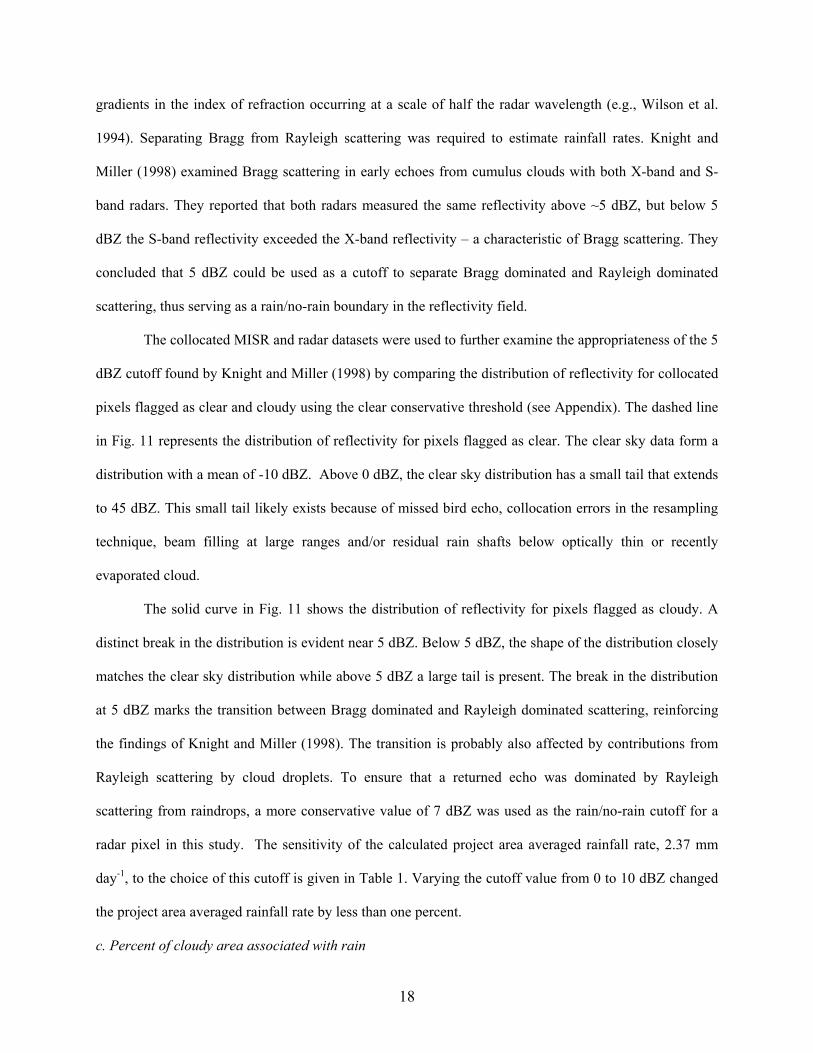
gradients in the index of refraction occurring at a scale of half the radar wavelength (e.g., Wilson et al.

1994). Separating Bragg from Rayleigh scattering was required to estimate rainfall rates. Knight and

Miller (1998) examined Bragg scattering in early echoes from cumulus clouds with both X-band and S-

band radars. They reported that both radars measured the same reflectivity above ~5 dBZ, but below 5

dBZ the S-band reflectivity exceeded the X-band reflectivity – a characteristic of Bragg scattering. They

concluded that 5 dBZ could be used as a cutoff to separate Bragg dominated and Rayleigh dominated

scattering, thus serving as a rain/no-rain boundary in the reflectivity field.

The collocated MISR and radar datasets were used to further examine the appropriateness of the 5

dBZ cutoff found by Knight and Miller (1998) by comparing the distribution of reflectivity for collocated

pixels flagged as clear and cloudy using the clear conservative threshold (see Appendix). The dashed line

in Fig. 11 represents the distribution of reflectivity for pixels flagged as clear. The clear sky data form a

distribution with a mean of -10 dBZ. Above 0 dBZ, the clear sky distribution has a small tail that extends

to 45 dBZ. This small tail likely exists because of missed bird echo, collocation errors in the resampling

technique, beam filling at large ranges and/or residual rain shafts below optically thin or recently

evaporated cloud.

The solid curve in Fig. 11 shows the distribution of reflectivity for pixels flagged as cloudy. A

distinct break in the distribution is evident near 5 dBZ. Below 5 dBZ, the shape of the distribution closely

matches the clear sky distribution while above 5 dBZ a large tail is present. The break in the distribution

at 5 dBZ marks the transition between Bragg dominated and Rayleigh dominated scattering, reinforcing

the findings of Knight and Miller (1998). The transition is probably also affected by contributions from

Rayleigh scattering by cloud droplets. To ensure that a returned echo was dominated by Rayleigh

scattering from raindrops, a more conservative value of 7 dBZ was used as the rain/no-rain cutoff for a

radar pixel in this study. The sensitivity of the calculated project area averaged rainfall rate, 2.37 mm

day-1, to the choice of this cutoff is given in Table 1. Varying the cutoff value from 0 to 10 dBZ changed

the project area averaged rainfall rate by less than one percent.

c. Percent of cloudy area associated with rain

18

Two cumulative frequency distributions showing the percent of cloudy area associated with

rainfall rates ranging from 0.1 mm hr-1 (5 dBZ) to 40 mm hr-1 (44 dBZ) are shown in Fig. 12. The lower

curve represents the cloud conservative cloud mask threshold and the upper curve represents the clear

conservative threshold (see Sec. 2). The figure shows that between 5.5% and 10.5% of the cloudy area

had rainfall rates greater than 0.1 mm hr-1 (i.e., approximately 90-95% of the cloudy area was not

producing detectable precipitation) and between 1.5% and 3.5% of the cloudy area had rainfall rates

greater than 1.0 mm h-1 (20 dBZ). Rainfall rates of 0.1 to 1 mm hr-1 are characteristic of drizzle (Glickman

2000). Figure 12 also shows that 0.25 to 0.5% of the cloudy area produced rainfall rates that exceeded 10

mm hr-1 (35 dBZ). Note that all clouds within the collocated scenes, cumulus, stratus, and cirrus, are

included in these statistics. Although cirrus were rare, stratus clouds, particularly remnants of previous

convection, were common.

d. Relationships between rainfall, cloud top height, and bi-directional reflectance factor

Figure 13 shows the distribution of MISR derived cloud-top heights measured in the area that

overlapped with the radar, the distribution of cloud-top heights for cloudy pixels containing detectable

rainfall (i.e., ≥ 7dBZ), and the ratio of these two distributions that gives the probability that a given cloud-

top height has detectable rain. Approximately 93% of the cloud tops were below 5250 m, an altitude near

the nominal height of the freezing level. 62% of cloudy pixels lie below 1750 m, of which less than 1%

had detectable rain. The pixels that have detectable rainfall occur most frequently with cloud-top heights

between 2250 m and 2750 m. The probability that a given cloud-top height has detectable rainfall rises

sharply for cloud tops in the 2250 – 2750 m bin, where 12% of these pixels have detectable rain. A steady

increase in this probability occurs, peaking at 22 % for the 5250 – 5750 m bin. Above 5750 m, this

probability drops sharply.

The probabilities given in Fig. 13 require careful interpretation, especially when comparing these

results to those of Byers and Hall (1955). Based on two airplanes flying in stacked formation – one

penetrating clouds to detect rain with an aircraft-mounted radar, the other measuring cloud-top heights –

Byers and Hall (1955) reported that none of the winter-time Caribbean clouds with cloud-top heights less

19

than 1.8 km were raining, half the clouds with tops between 2.7 and 3.0 km were raining, and all the

clouds with tops greater than 3.5 km were raining. There are two key reasons why the results of Fig. 13

differ from those of Byers and Hall (1955). The first is that the Byers and Hall results use a rain-per-cloud

analysis, while the results of Figure 13 use a rain-per-pixel (1.1 km resolution) analysis. Thus our results

reflect the fraction of cloud area that is raining within a given height range, while the Byers and Hall

results reflect the fraction of cloud cells that are raining within a given height range. The second reason

for the difference is that the two airplanes used in the Byers and Hall results only sampled clouds all

having the same cloud base near the lifting condensation level (LCL). Our analysis included all clouds

within the MISR and radar collocated domain. The forward video camera mounted on the C-130 aircraft

during RICO showed that not all clouds had their base near the LCL; geometrically thin clouds over a

large range of cloud-base altitudes are apparent in the video. These geometrically thin clouds, which we

can assume are not raining, reduce the probability that a pixel within a given cloud-top height range has

detectable rain. The sharp drop in this probability above 5750 m (Fig. 13) is attributed to these

geometrically thin clouds dominating the cloud type above 5750 m.

Figure 14 shows the joint relationships between radar-estimated rainfall rate, MISR cloud-top

height, and the MISR 866 nm BRF. The BRFs were taken from the nadir camera under solar zenith

angles ranging from 39.13° to 49.58°. Figure 14a shows the distribution in the total number of pixels that

have detectable rainfall as a function of cloud-top height and BRF. Note that collocated pixels with

detectable rain (≥ 7dBZ) and with cloud tops ~ 2.5 km in altitude and moderately bright reflectance (BRF

0.4 to 0.8) have the highest frequency of occurrence. Figure 14b shows the distribution of average

rainfall rate (mm hr-1) for cloudy pixels having detectable rainfall as a function of cloud-top height and

BRF. Note that at any given cloud-top height, the brightest clouds had the highest rainfall rates. Figure

14c depicts the distribution of summed rainfall rates as a function of cloud-top height and BRF, showing

that half the total rainfall comes from clouds with cloud-top altitudes between 2750 and 4250 m and with

BRFs between 0.4 and 1.0. Figure 14 also shows that there are cases of detectable rainfall even for low (<

0.2) BRF clouds. This may be due to the small errors in geolocating radar and MISR data (Section 2),

20

cloud-on-cloud shadowing of the incident sunlight causing low BRF values for cloudy pixels (e.g., as

recently demonstrated in Yang and Di Girolamo (2008) for boundary layer cumuli), or clouds toward the

end of their lifecycle. This later possibility is subjectively confirmed based on our aircraft experience

during RICO, where we occasionally visually noted light rain where little to no clouds existed above.

A careful look at Fig. 14b also reveals that the average rainfall rate increases with cloud-top

height over a large portion of the altitude range. This is better seen in Fig. 15, which shows the average

rainfall rate for all pixels with detectable rainfall (≥ 7 dBZ) as a function of cloud top height. The largest

number of samples occurs between cloud-top heights of 1250 m and 3750 m. In this range of cloud-top

heights, we see that the average rainfall rates increase almost linearly with cloud-top height. Above and

below this range, the number of samples drops substantially, limiting our confidence in the estimate of the

average rainfall rate. The standard deviation of the average rainfall rate is also given in Fig. 15. Note the

standard deviation is large and increases with increasing height in the range of 1250 – 3750 m. The large

standard deviation arises from long tails in the rainfall rate distributions that stretch to large rainfall rates.

7. Mesoscale cloud organization

Figure 7 shows significant day-to-day variability in dR . Visual inspection of the collocated radar

and MISR data (e.g., Fig. 5), as well as collocated radar and visible GOES imagery over the entire 62

days of radar operation, revealed that cloud organization on the mesoscale was clearly related to

precipitation intensity and distribution. Figures 16a-c show three examples of the mesoscale organization

of clouds observed during RICO. The wind-parallel cloud streets appearing on Fig. 16a were very

common, but visual inspection of the collocated datasets showed that they rarely produced detectable

rainfall (≥ 7dBZ). Figure 16b shows a second type of cloud organization that is characterized by small

clusters of trade wind cumuli. While not as common as the wind parallel clouds, these clusters often had

light to moderate rainfall rates. Nearly all of the clouds that were found to be producing significant

precipitation appeared to be associated with shallow cumulus clusters aligned in arc-shaped formations

reminiscent of cold pool outflows documented in many studies of deep tropospheric convection (e.g.

21

Tompkins 2001). The clouds along these arcs, as shown Figs. 16c and 5a, typically extended no higher

than the freezing level (~ 5 km) and were often shallower. Tompkins (2001) reported that the role of

propagating cold pools was important to the spatial organization of tropical deep convection. This

conclusion appears to translate to the shallow precipitating clouds observed during RICO, including

remnant thin clouds at the center of the cold pool (cf. Fig. 14 of Tompkins 2001).

8. Conclusions

In this paper, characteristics of trade-wind clouds and precipitation were investigated using S-

band radar and aircraft data from the Rain In Cumulus over the Ocean (RICO) field campaign and high-

resolution satellite data from the Multiangle Imaging SpectroRadiometer (MISR). The major findings of

this study are as follows:

1. A Z-R relationship was derived and found to be Z = 88.0R1.50. The Z-R relationship from RICO

provided an estimate of total project precipitation that was 18% higher than if calculated using the Stout

and Mueller (1968) relationship from data in “trade wind showers” collected in the Marshall Islands.

2. The area averaged rainfall rate for RICO was 2.37 mm day-1. Daily rainfall rates varied from 0

to 22 mm day-1 with the majority of the days having rainfall rates between 0.5 and 3 mm day-1. Nearly

42% of the total rain that fell during RICO occurred during the three rainiest days and 56% on the six

rainiest days. Only 9% fell in the driest 31 days.

3. A correction to account for evaporation below cloud base was estimated. Evaporation was

shown to be strongly dependent on the drop size distribution and the corresponding rainfall rate. At most,

we recommend a 6% reduction in rainfall to account for evaporation below cloud base. Using this

estimate, the average surface rainfall rate for the 62 days of the RICO project would reduce to 2.23 mm

day-1.

4. When compared to TRMM (Tropical Rainfall Measurement Mission) estimates of precipitation

during December 2004 and January 2005 (the RICO period) over the same region, the 3B43 “Best

Estimate” precipitation product reported a surface rainfall rate of 1.05 mm day-1. Differences between the

TRMM precipitation estimate and the estimates reported here can be attributed primarily to the different

22

Z-R relationship used by TRMM’s precipitation radar (PR), the PR’s reduced sensitivity (minimum

detectable echo of 17 dBZ), the differences in sampling (both time and space), and the other sources of

data used in the 3B43 algorithm which include rain gauges, infrared brightness temperatures and

microwave emissions (see Stephens and Kummerow 2007 for a discussion of issues related to space-

based precipitation estimates). If one adjusts our rainfall statistics by applying the TRMM Z-R

relationship for shallow convection (Z=147.5R1.554), accounting for the reduced sensitivity, and adjusting

the rainfall rate for evaporation below cloud base, the RICO area averaged surface rainfall rate was 1.38

mm day-1, about 23% higher than the TRMM estimate.

The GPCP (Global Precipitation and Climatology Project) V2 precipitation product reported 1.25

mm day-1. The values reported in this paper are about a factor of two larger. These differences are

attributable to a number of factors that are commonly acknowledged as shortcomings in space-based

precipitation estimates (e.g., Stephens and Kummerow 2007).

5. The area averaged surface rainfall rate of 2.23 mm day-1 corresponds to a latent heat flux of 63

Wm-2. This flux represents the local return of water to the ocean surface through precipitation. When

compared to the wintertime ocean-surface latent heat flux of Chou et al. (1995), the daily averaged return

of water to the ocean through precipitation processes within the trade wind layer during RICO was 31-

39%.

6. A diurnal cycle was observed in the area averaged rainfall rate. The magnitude of the rainfall

and the frequency of its occurrence had a maximum in the pre-dawn hours and minimum in the mid-

morning to early afternoon. The magnitude of the rainfall and the frequency of its occurrence had a

maximum in the pre-dawn hours and minimum in the mid-morning to early afternoon on 64% of the days.

7. Comparison of the collocated radar estimated precipitation and the MISR derived cloud field

revealed that between 5.5-10.5% of the cloudy area had rainfall rates > 0.1 mm hr-1 (5 dBZ) and between

1.5-3.5% of the cloudy area had rainfall rates greater than 1.0 mm hr-1 (20 dBZ). When stratified by

cloud-top height, 12% of the MISR pixels having cloud tops in the 2250 – 2750 m range had detectable

rainfall rates, increasing to 22% for cloud tops in the 5250 – 5750 m range.

23

8. Comparison of the collocated radar estimated precipitation and the MISR derived cloud-top

heights and near-IR BRFs showed the dominant height of clouds with rainfall rates > 0.1 mm hr-1 was

between 2250-2750 m. At any given cloud-top height, the brightest clouds have the highest rainfall rates.

Observations of raining clouds having low BRFs were also noted. Clouds with cloud-top heights between

~3 and 4 km and BRFs between 0.4 and 1.0 contributed ~50% to the total rainfall. For cloudy pixels

having detectable rain, average surface rainfall rates increased from ~1 mm hr-1 to ~4 mm hr-1 as cloud-

top heights increased from ~1 km to 4 km.

9. Rainfall rates were closely tied to the type of mesoscale organization. Very little of the total

rainfall was associated with clouds organized into wind-parallel streets. Much of the rainfall came from

cumulus clusters aligned in arc-shaped formations associated with cold pool outflows.

24

Acknowledgements

This research was supported by the National Science Foundation (NSF) under grant ATM-03-46172 and

from contract 121756 with the Jet Propulsion Laboratory (JPL), California Institute of Technology. Any

opinions, findings and conclusions or recommendations expressed in this publication are those of the

authors and do not necessarily reflect the views of the NSF, JPL, or the University of Illinois. We would

also like to acknowledge the contributions of Matt Freer, Sabine Göke, Lusheng Liang, Hilary Minor,

Robert Rilling and Guangyu Zhao. We especially thank the RICO team, particularly the NCAR SPolKa

radar team and the C-130 Scientists and staff for their efforts. We also thank Charles Knight and an

anonymous reviewer for reviews that led to substantial improvements in the paper.

25

Appendix

Date MISR

Orbit number*

Cloud Fraction

in collocate

d area

MISR clear conservative

(cloud conservative)

BRF Threshold

SPolKa Time

(UTC)

Rawinsonde Time (location)

11/26/04 26289 51.10% 0.025 (0.075) 14:51:48 12UTC (Guadeloupe)

11/28/04 26318 21.60% 0.024 (0.072) 14:40:39 12UTC (Guadeloupe)

12/7/04 26449 36.70% 0.024 (0.072) 14:35:47 12UTC (Guadeloupe)

12/12/04 26522 41.40% 0.026 (0.078) 14:54:35 10:48UTC (Barbuda)

12/14/04 26551 58.10% 0.026 (0.078) 14:42:24 10:51UTC (Barbuda)

12/21/04 26653 19.90% 0.024 (0.072) 14:47:33 10:59UTC (Barbuda)

12/28/04 26755 77.80% 0.026 (0.078) 14:52:29 10:57UTC (Barbuda)

12/30/04 26784 44.80% 0.024 (0.072) 14:49:26 10:57UTC (Barbuda)

1/6/05 26886 53.90% 0.025 (0.075) 14:48:11 16:56UTC (Barbuda)

1/13/05 26988 84.30% 0.04 (0.120) 14:55:31 14:03UTC (Barbuda)

1/15/05 27017 49.90% 0.034 (0.102) 14:42:37 16:59UTC (Barbuda)

1/22/05 27119 48.90% 0.024 (0.072) 14:48:12 16:45UTC (Barbuda)

1/24/05 27148 49.10% 0.025 (0.075) 14:36:38 16:46UTC (Barbuda)

* MISR block range 74-78

26

References Adler, R. F., G. J. Huffman, A. Chang, R. Ferraro, P.-P. Xie, J. Janowiak, B. Rudolf, U. Schneider, S.

Curtis, D. Bolvin, A. Gruber, J. Susskind, P. Arkin, and E. Nelkin, 2003: The version-2 Global

Precipitation Climatology Project (GPCP) Monthly Precipitation Analysis (1979-Present). J.

Hydrometeor., 4, 1147-1167.

Albrecht, B.A., C.S. Bretherton, D. Johnson, W.H. Scubert, and A.S. Frisch, 1995: The Atlantic

Stratocumulus Transition Experiment—ASTEX. Bull. Amer. Meteor. Soc., 76, 889–904.

Augstein, E, H. Riehl, F. Ostapoff, and V. Wagner, 1973: Mass and energy transports in an undisturbed

Atlantic trade-wind flow. Mon. Wea. Rev., 101, 101-111

Battan, L.J., and R.R. Braham, 1956: A study of convective precipitation based on cloud and radar

observations. J. Atmos. Sci., 13, 587–591.

Betts, A. K., 1997: The physics and parameterization of moist atmospheric convection. Chapter 4: Trade

Cumulus: Observations and Modeling. pp. 99-126. Dordrecht, The Neth.: Kluwer.

Browning, K. A. and R. Wexler, 1968: A determination of kinematic properties of a wind field using

Doppler radar. J. Appl. Meteor., 7, 105-113.

Bruegge, C. J., D. J. Diner, R. A. Kahn, N. Chrien, M. C. Helmlinger, B. J. Gaitley, and W. A. Abdou,

2007: The MISR radiometric calibration process. Rem. Sens. Environ., 107 (1-2): 2.

doi:10.1016/j.rse.2006.07.024.

Byers, H.R., and R.K. Hall, 1955: A census of cumulus-cloud height versus precipitation in the vicinity of

Puerto Rico during the winter and spring of 1953-1954. J. Atmos. Sci., 12, 176–178.

Chou, S.H., R.M. Atlas, C.L. Shie, and J. Ardizzone, 1995: Estimates of surface humidity and latent heat

fluxes over oceans from SSM/I Data. Mon. Wea. Rev., 123, 2405–2425.

Diner, D.J., J.C. Beckert, T.H. Reilly, C.J. Bruegge, J.E. Conel, R. Kahn, J.V. Martonchik, T.P.

Ackerman, R. Davies, S.A.W. Gerstl, H.R. Gordon, J-P. Muller, R. Myneni, R.J. Sellers, B. Pinty,

and M.M. Verstraete, 1998: Multi-angle Imaging SpectroRadiometer (MISR) description and

experiment overview. IEEE Trans. Geosci. Rem. Sens., 36 (4), 1072-1087.

27

Diner, D.J., Beckert, J.C., Bothwell, G.W. and Rodriguez, J.I., 2002: Performance of the MISR

instrument during its first 20 months in Earth orbit. IEEE Trans. Geosci. Remote Sensing. 40 (7),

1449-1466.

Doviak, R. J., and D. S. Zrnić, 1993: Doppler Radar and Weather Observations. Academic Press, 458 pp.

Genkova, I., G. Seiz, P. Zuidema, G. Zhao and L. Di Girolamo, 2007: Cloud-top height comparisons from

ASTER, MISR, and MODIS for trade wind cumuli. Remote Sens. Environ., 107, 211-222.

Glickman, T. S., 2000: Glossary of Meteorology. American Meteorological Society, Boston MA, 855 pp.

Hahn, C.J., and S.G. Warren, 1999: Extended edited cloud reports from ships and land stations over the

globe, 1952-1996. Numerical data package NDP-026C, Carbon Dioxide Information Analysis

Center (CDIAC), Department of Energy, Oak Ridge, Tennessee (Documentation, 79 pages).

Heymsfield, A. J., and J. L. Parrish, 1979: Techniques employed in the processing of particle size spectra

and state parameter data obtained with the T-28 aircraft platform. NCAR Tech. Note NCAR/TN-

137 +1A, 78 pp.

Heymsfield, A., and D. Baumgardner, 1985: Summary of a workshop on processing of 2D probe data.

Bull. Amer. Meteor. Soc., 66, 437–440.

Holland, J.Z., 1970: Preliminary report on the BOMEX sea-air interaction program. . Bull. Amer. Meteor.

Soc., 51, 809-820.

Houze Jr, R.A., S. Brodzik, C. Schumacher, S.E. Yuter, and C.R. Williams, 2004: Uncertainties in

oceanic radar rain maps at Kwajalein and implications for satellite validation. J. Appl. Meteor., 43,

1114–1132.

Huffman, G.J., R. F. Adler, P. Arkin, A. Chang, R. Ferraro, A. Gruber, J. Janowiak, A. McNab, B. Rudolf

and U. Schneider 1997: The Global Precipitation Climatology Project (GPCP) Combined

Precipitation Dataset. Bull. Amer. Meteor. Soc., 78, 5-20.

Iguchi, T., T. Kozu, R. Meneghini, J. Awaka, and K. Okamoto, 2000: Rain-Profiling algorithm for the

TRMM Precipitation Radar. J. Appl. Meteor., 39, 2038–2052.

28

Ikai, J., and K. Nakamura, 2003: Comparison of rain rates over the ocean derived from TRMM

Microwave Imager and Precipitation Radar. J. Atmos. Oceanic Technol., 20, 1709–1726.

Jovanovic, V.M., Bull, M.A., Smyth, M.M. and J. Zong, 2002: MISR in-flight camera geometric model

calibration and georectification performance. IEEE Trans. Geosci. Remote Sensing. 40 (7), 1512-

1519.

Knight, C.A., and L.J. Miller, 1998: Early radar echoes from small, warm cumulus: Bragg and

hydrometeor scattering. J. Atmos. Sci., 55, 2974–2992.

Korolev, A., 2007: Reconstruction of the sizes of spherical particles from their shadow images. Part I:

theoretical considerations. J. Atmos. Oceanic Technol., 24, 376–389.

Kuettner, J. P., D. E. Parker, D. R. Rodenhuis, H. Hoeber, H. Kraus, and S. G. H. Philander, 1974:

GATE. Bull. Amer. Meteor. Soc., 55, 711-744.

Liu, G., J. A. Curry, and R.-S. Sheu 1995: Classification of clouds over the western equatorial Pacific

Ocean using combined infrared and microwave satellite data. J. Geophys. Res., 100, NO. D7,

13811-13826.

Loomis, E., 1882: Contributions to meteorology: Being results derived from an examination of

observations of the United States Signal Service and from other sources. Amer. J. Sci., 23, 1-25.

Marchand, R. T., T. P. Ackerman, and C. Moroney, 2007: An assessment of multi-angle imaging

spectroradiometer (MISR) stereo-derived cloud-top heights and cloud-top winds using ground-

based radar, lidar, and microwave radiometers. J. Geophys. Res. 112, D06204,

doi:10.1029/2006JD007091.

Minnis, P., 1989: Viewing zenith angle dependence of cloudiness determined from coincident GOES East

and GOES West data. J. Geophys. Res., 94, D2, 2303–2320.

Moroney, C., R. Davies, and J.-P. Muller, 2002: Operational retrieval of cloud-top heights using MISR

data. IEEE Trans. Geosci. Remote Sens., 40, 1532-1540.

29

Naud, C. M., J-P. Muller, E. E. Clothiaux, B. A. Baum and W. P. Menzel. 2005: Intercomparison of

multiple years of MODIS, MISR and radar cloud-top heights. Annales Geophysicae 23 (7): 2415-

2424.

Nesbitt, S.W., and E.J. Zipser, 2003: The diurnal cycle of rainfall and convective intensity according to

three years of TRMM measurements. J. Climate, 16, 1456–1475.

Nesbitt, S.W., E.J. Zipser, and C.D. Kummerow, 2004: An examination of version-5 rainfall estimates

from the TRMM Microwave Imager, Precipitation Radar, and rain gauges on global, regional, and

storm scales. J. Appl. Meteor., 43, 1016–1036.

Oye, R., C. Mueller, and S. Smith, 1995: Software for radar translation, visualization, editing, and

interpolation. Preprints, 27th Conf. Radar Meteorology, Vail CO, Amer. Meteor. Soc., 359-361.

Petty, G., 1999: Prevalence of precipitation from warm-topped clouds over eastern Asia and the western

Pacific. J. Climate, 12, 220-229.

Rauber, R. M., N. F. Laird, and H. T. Ochs III, 1996; Precipitation efficiency of trade wind clouds over

the north central tropical Pacific Ocean. J. Geophys. Res., 101, D21, 26247-26253.

Rauber, R.M., B. Stevens, H.T. Ochs, C. Knight, B.A. Albrecht, A.M. Blyth, C.W. Fairall, J.B. Jensen,

S.G. Lasher-Trapp, O.L. Mayol-Bracero, G. Vali, J.R. Anderson, B.A. Baker, A.R. Bandy, E.

Burnet, J.L. Brenguier, W.A. Brewer, P.R.A. Brown, P. Chuang, W.R. Cotton, L. Di Girolamo, B.

Geerts, H. Gerber, S. Göke, L. Gomes, B.G. Heikes, J.G. Hudson, P. Kollias, R.P. Lawson, S.K.

Krueger, D.H. Lenschow, L. Nuijens, D.W. O'Sullivan, R.A. Rilling, D.C. Rogers, A.P. Siebesma,

E. Snodgrass, J.L. Stith, D.C. Thornton, S. Tucker, C.H. Twohy, and P. Zuidema, 2007: Rain in

shallow cumulus over the ocean. Bull. Amer. Meteor. Soc., 88, 1912–1928.

Riehl, H, T. C. Yeh, J. S. Malkus, and N. E. LaSeur, 1951: The northeast trade of the Pacific Ocean.

Quart. J. Roy. Meteor. Soc., 77, 598–626.

Rogers, R.R., and M. K. Yau, 1989: A short course in cloud physics. 3rd. Edition, Pergamon Press, 293

pp.

30

Rossow, W.B., and R.A. Schiffer, 1999: Advances in understanding clouds from ISCCP. Bull. Amer.

Meteor. Soc., 80, 2261–2287.

Short, D. A., and K. Nakamura, 2000: TRMM radar observations of shallow precipitation over the

tropical oceans. J. Climate, 13, 4107-4124.

Siebesma, A. P., 1998: Shallow cumulus convection. Buoyant Convection in Geophysical Flows, Vol.

513, E. J. Plate, et al., Eds., Kluwer Academic, 441-486.

Snodgrass, E. R., 2006: Precipitation characteristics of trade wind clouds during RICO derived from

radar, satellite, and aircraft measurements. Masters Thesis, Department of Atmospheric Sciences,

University of Illinois at Urbana-Champaign, 105 S. Gregory St., Urbana, IL 61801. 101 pp.

Stephens, G.L., and C.D. Kummerow, 2007: The Remote sensing of clouds and precipitation from space:

a review. J. Atmos. Sci., 64, 3742–3765.

Stevens, B., 2005: Atmospheric Moist Convection. Annual Rev. Earth Planet Sci., 33, 605- 643.

Stout, G.E., and E.A. Mueller, 1968: Survey of relationships between rainfall rate and radar reflectivity in

the measurement of precipitation. J. Appl. Meteor., 7, 465–474.

Tompkins, A.M., 2001: Organization of tropical convection in low vertical wind shears: the role of cold

pools. J. Atmos. Sci., 58, 1650–1672.

Webster, P.J., and R. Lukas, 1992: TOGA COARE: The Coupled Ocean—Atmosphere Response

Experiment. Bull. Amer. Meteor. Soc., 73, 1377–1416.

Wielicki, B.A., and R.M. Welch, 1986: Cumulus cloud properties derived using Landsat satellite data. J.

Appl. Meteor., 25, 261–276.

Wilson, J.W., T.M. Weckwerth, J. Vivekanandan, R.M. Wakimoto, and R.W. Russell, 1994: Boundary

layer clear-air radar echoes: origin of echoes and accuracy of derived winds. J. Atmos. Oceanic

Tech., 11, 1184–1206.

Xie, P., and P.A. Arkin, 1997: Global precipitation: a 17-year monthly analysis based on gauge

observations, satellite estimates, and numerical model outputs. Bull. Amer. Meteor. Soc., 78, 2539–

2558.

31

Yang, Y., and L. Di Girolamo, 2008: Impacts of 3-D radiative effects on satellite cloud detection and their

consequences on cloud fraction and aerosol optical depth retrievals. J. Geophys. Res. (In Press).

Zhao, G., and L. Di Girolamo, 2004: A cloud fraction versus view angle technique for automatic in-scene

evaluation of the MISR cloud mask. J. Appl. Meteor., 43, 860–869.

Zhao, G., and L. Di Girolamo, 2006: Cloud fraction errors for trade wind cumuli from EOS- Terra

instruments. Geophys. Res. Lett., 33, L.20802, doi: 10.1029/2006GL027088, 2006.

Zhao, G., and L. Di Girolamo, 2007: Statistics on the macrophysical properties of trade wind cumuli over

the tropical western Atlantic. J. Geophys. Res., 112, D10204, doi:10.1029/2006JD007371, 2007.

32

Table 1 Sensitivity of project area averaged rainfall rate to rain/no-rain reflectivity cutoff

Cutoff (dBZ) Rainfall Rate (mm day-1)

-5 2.44 0 2.41 5 2.38 7 2.37

10 2.34 17 2.22

33

Figure Captions Figure 1. Z-R relationship calculated from the droplet spectra determined from the C-130 2DP and 2DC

optical array probes from passes through rain shafts on Research Flight 17 on 19 Jan 2005 during

RICO (dark solid line). Each dot represents one rain shaft. Also graphed is the Z-R relationship

from trade wind showers measured by Stout and Mueller (1968).

Figure 2 Radar images from a precipitation free region on 12 December 2004 that illustrate the filtering of

bird, noise and island echoes. a) Original reflectivity field (dBZ); b) Reflectivity field with the

island of Barbuda removed; c) Reflectivity field with island removed, and automated noise and

bird filter applied; d) same as (c) but with additional manual editing to remove remaining bird

echo (only applied to the collocated MISR scenes).

Figure 3. Geometry of the 0.5° scan of the radar beam relative to a typical precipitating trade wind

cumulus cloud. (Top) View along the beam showing the beam width and height. (Bottom Left)

0.5° vertical beam geometry as a function of arc distance along the Earth’s surface. (Bottom

Right) Range gate width and height. The dashed square box on the top image and darker yellow

shading in the lower left image highlight the range of 25-90 km used in this paper.

Figure 4. A) Rain Fraction (%), defined as the number of post-filtered pixels with reflectivity ≥ 7 dBZ

divided by the total number of pixels per annulus less those marked as birds, sun spikes, bad

beams and islands. B) Average reflectivity (dBZ). C) Rain Area (m2). These variables are plotted

for each of the 5 km annuluses.

Figure 5. 14 December 2004 1442 UTC. (A) MISR nadir camera RGB image. (B) MISR nadir camera

cloud mask (clear conservative); (C) SPolKa reflectivity (dBZ) post-filtered and interpolated to

the MISR grid. (D) Same as (C) but superimposed on image (B). Yellow circles denoted the

maximum range of the radar (147 km).

Figure 6. Number of 0.5° scans per half hour on each RICO day.

34

Figure 7. (A) Daily area averaged rainfall rate ( dR , mm day-1) in chronological order. (B) dR sorted from

rainiest to least rainiest day and a cumulative frequency distribution of dR . Dates outlined in

black are those in which coincident MISR data was available. The Z-R relationship shown in Fig.

1 was derived from data collected during RF-17 on 19 Jan 2005 as indicated on (A) and (B).

Figure 8. The diurnal cycle of precipitation during RICO. (A) Area averaged rainfall rate, hR (mm day-1)

using all available data (solid line), and with the 6 rainiest and 6 least rainiest days removed

(dashed line). (B) (Solid) The number of times that a half-hour interval was one of the top three

rainiest half-hour intervals of the day, summed for the entire project. (Dashed) The number of

times that a half-hour interval was one of the three least rainy half-hour intervals of the day,

summed for the entire project. Both lines in (B) are three-hour moving averages.

Figure 9. (Solid line) Cumulative frequency diagram for all days of the RICO project showing the

difference between the average rainfall rate during the three hour period centered on the early

morning (7 AM LT) maximum in Figure 8a and the three hour period centered on the mid-

morning (10:30 AM LT) minimum. (Bars at right) Rainfall rate on each day of the project, with

the days aligned to correspond to their position on the cumulative frequency diagram.

Figure 10: (Points) Percent reduction in rainfall rate and reflectivity at the ocean surface as a function of

the original rainfall rate and reflectivity at cloud base for each of the drop spectra measured

during rain shaft penetrations on Research Flight 17 19 Jan 2005 during RICO (see Fig. 1). (Dark

line) Least-squares fit to the data (equation and correlation coefficient in upper right corner).

(Vertical gray shaded line) average reflectivity (26.7 dBZ) and corresponding rainfall rate (3.0

mm hr-1) determined over the range 25-90 km from Fig. 4B. The horizontal gray line marks the

percent reduction that corresponds to the point where the vertical gray line crosses the least-

squares fit.

Figure 11. The number of collocated pixels that were determined to be clear (dashed) and cloudy (solid)

by MISR as a function of radar reflectivity.

35

Figure 12. Cumulative frequency distribution of the percent of cloudy area associated with a rainfall rate,

R, greater than R. The gray envelope represents the uncertainty in cloud cover due to different

cloud detection thresholds. The bottom (top) of the envelope represents the cloud (clear)

conservative threshold.

Figure 13. a: MISR “Best Winds” stereo cloud-top height distribution for clouds within the radar domain

binned every 500 m starting at 250 m. b: the number of post-filtered collocated radar pixels with

reflectivity ≥7 dBZ as a function of cloud-top height. c: The ratio b/a, which represents the

probability that a given cloud-top height has detectable rain.

Figure 14. MISR-derived cloud-top height and BRF are plotted against, (A) the number of post-filtered

collocated radar pixels with reflectivity ≥7 dBZ, (B) average rainfall rate, and (C) the summed

rainfall rate for all post-filtered, collocated radar data.

Figure 15. (Left) The average rainfall rate as a function of cloud-top height for pixels with detectable

rainfall rates (≥7 dBZ). The numbers are the standard deviation. Bins are 500 m thick, beginning

at 250 m. (Right) number of pixels included in the average.

Figure 16. Typical cloud mesoscale organization. (A) wind parallel cloud streets. (B) small cumulus

clusters. (C) cumulus clusters along propagating cold pools.

36

Fig. 1. Z-R relationship calculated from the droplet spectra determined from the C-130 2DP and 2DC optical array probes from passes through rain shafts on Research Flight 17 on 19 Jan 2005 during RICO (dark solid line). Each dot represents one rain shaft. Also graphed is the Z-R relationship from trade wind showers measured by Stout and Mueller (1968).

37

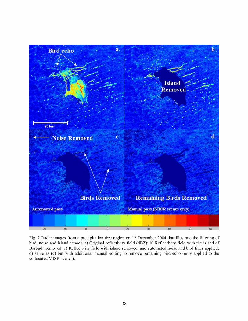
Fig. 2 Radar images from a precipitation free region on 12 December 2004 that illustrate the filtering of bird, noise and island echoes. a) Original reflectivity field (dBZ); b) Reflectivity field with the island of Barbuda removed; c) Reflectivity field with island removed, and automated noise and bird filter applied; d) same as (c) but with additional manual editing to remove remaining bird echo (only applied to the collocated MISR scenes).

38

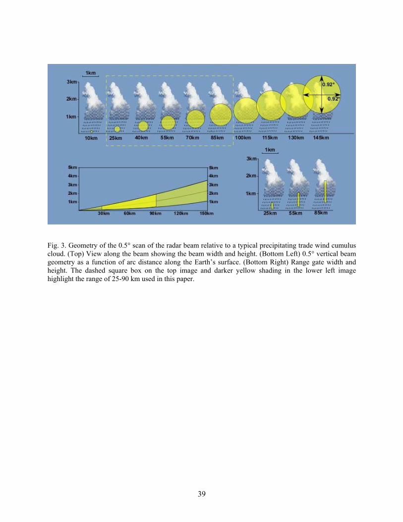
Fig. 3. Geometry of the 0.5° scan of the radar beam relative to a typical precipitating trade wind cumulus cloud. (Top) View along the beam showing the beam width and height. (Bottom Left) 0.5° vertical beam geometry as a function of arc distance along the Earth’s surface. (Bottom Right) Range gate width and height. The dashed square box on the top image and darker yellow shading in the lower left image highlight the range of 25-90 km used in this paper.

39

Fig. 4. A) Rain Fraction (%), defined as the number of post-filtered pixels with reflectivity ≥ 7 dBZ divided by the total number of pixels per annulus less those marked as birds, sun spikes, bad beams and islands. B) Average reflectivity (dBZ). C) Rain Area (m2). These variables are plotted for each of the 5 km annuluses.

40

Fig. 5. 14 December 2004 1442 UTC. (A) MISR nadir camera RGB image. (B) MISR nadir camera cloud mask (clear conservative); (C) SPolKa reflectivity (dBZ) post-filtered and interpolated to the MISR grid. (D) Same as (C) but superimposed on image (B). Yellow circles denoted the maximum range of the radar (147 km).

41

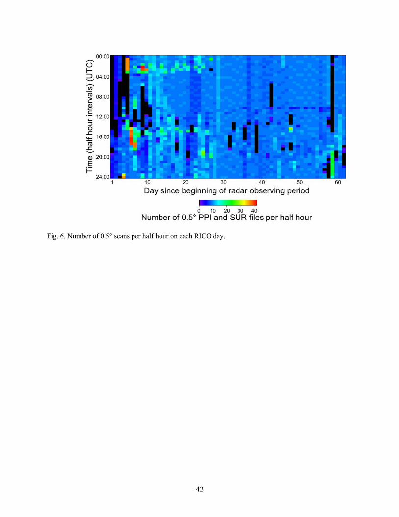
Fig. 6. Number of 0.5° scans per half hour on each RICO day.

42

Fig. 7. (A) Daily area averaged rainfall rate ( dR , mm day-1) in chronological order. (B) dR sorted from rainiest to least rainiest day and a cumulative frequency distribution of dR . Dates outlined in black are those in which coincident MISR data was available. The Z-R relationship shown in Fig. 1 was derived from data collected during RF-17 on 19 Jan 2005 as indicated on (A) and (B).

43

Fig. 8. The diurnal cycle of precipitation during RICO. (A) Area averaged rainfall rate, hR (mm day-1) using all available data (solid line), and with the 6 rainiest and 6 least rainiest days removed (dashed line). (B) (Solid) The number of times that a half-hour interval was one of the top three rainiest half-hour intervals of the day, summed for the entire project. (Dashed) The number of times that a half-hour interval was one of the three least rainy half-hour intervals of the day, summed for the entire project. Both lines on (B) are three-hour moving averages.

44

Fig. 9. (Solid line) Cumulative frequency diagram for all days of the RICO project showing the difference between the average rainfall rate during the three hour period centered on the early morning (7 AM LT) maximum in Figure 8a and the three hour period centered on the mid-morning (10:30 AM LT) minimum. (Bars at right) Rainfall rate on each day of the project, with the days aligned to correspond to their position on the cumulative frequency diagram.

45

Fig. 10. Percent reduction in rainfall rate and reflectivity at the ocean surface as a function of the original rainfall rate and reflectivity at cloud base for each of the drop spectra measured during rain shaft penetrations on Research Flight 17 on 19 Jan 2005 during RICO (see Fig. 1). The dark line is the least-squares fit to the data (equation and correlation coefficient in upper right corner). The vertical gray shaded line is the average reflectivity (26.7 dBZ) and corresponding rainfall rate (3.0 mm hr-1) determined over the range 25-90 km from Fig. 4B. The horizontal gray line marks the percent reduction that corresponds to the point where the vertical gray line crosses the least-squares fit.

46

Fig. 11. The number of collocated pixels that were determined to be clear (dashed) and cloudy (solid) by MISR as a function of radar reflectivity.

47

Fig. 12. Cumulative frequency distribution of the percent of cloudy area associated with a rainfall rate, R, greater than R. The gray envelope represents the uncertainty in cloud cover due to different cloud detection thresholds. The bottom (top) of the envelope represents the cloud (clear) conservative threshold.

48

Fig. 13. a: MISR “Best Winds” stereo cloud-top height distribution for clouds within the radar domain binned every 500 m starting at 250 m. b: the number of post-filtered collocated radar pixels with reflectivity ≥7 dBZ as a function of cloud-top height. c: The ratio b/a, which represents the probability that a given cloud-top height has detectable rain.

49

A

Fig. 14. MISR-derived cloud-top height and BRF are plotted against, (A) the number of post-filtered collocated radar pixels with reflectivity ≥7 dBZ, (B) average rainfall rate, and (C) the summed rainfall rate for all post-filtered, collocated radar data.

C

50

Fig. 15. (Left) The average rainfall rate as a function of cloud-top height for pixels with detectable rainfall rates (≥7 dBZ). The numbers are the standard deviation. Bins are 500 m thick, beginning at 250 m. (Right) number of pixels included in the average.

51

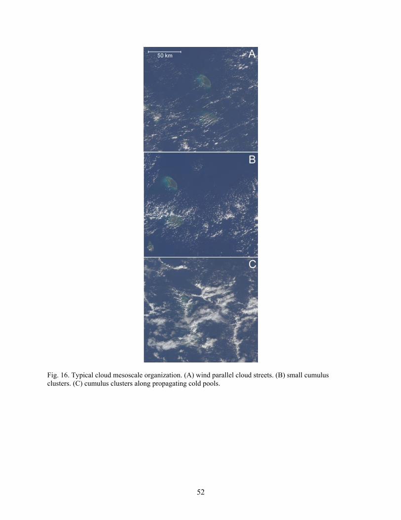
Fig. 16. Typical cloud mesoscale organization. (A) wind parallel cloud streets. (B) small cumulus clusters. (C) cumulus clusters along propagating cold pools.

52