preceding vehicle dynamics modeling for fuel efficient ...1049394/fulltext01.pdf · preceding...
TRANSCRIPT
IN DEGREE PROJECT ELECTRICAL ENGINEERING,SECOND CYCLE, 30 CREDITS
, STOCKHOLM SWEDEN 2016
Preceding Vehicle Dynamics Modeling for Fuel Efficient Control Strategies
PAWEL KUPSC
KTH ROYAL INSTITUTE OF TECHNOLOGYSCHOOL OF ELECTRICAL ENGINEERING

Preceding Vehicle Dynamics Modeling for FuelEfficient Control Strategies
An explorative study of speed prediction methods for heavy duty vehicles.
PAWEL KUPSC
Master’s Thesis at the Department of Automatic Control at KTHSupervisor at KTH: Afrooz Ebadat
Supervisors in Industry: Assad Alam, Per SahlholmExaminer: Cristian Rojas
TRITA-EE 2016-122

AbstractLong haulage trucks are a key part of today’s goods trans-port networks. To reduce fuel costs and emissions fromtrucks, novel methods of regulating their speed optimallybased on road slope data and other vehicles’ behavior arebeing developed. An important ability for these systems,when there is no vehicle to vehicle communication, is to beable to anticipate the speed of the vehicle driving in front.
This master thesis explores a number of possible ap-proaches of predicting the speed of a preceding heavy ve-hicle. The work is limited to vehicles controlled by one oftwo common speed control systems: cruise control (CC)and look ahead cruise control (LACC) when driving on ahighway. Initially, general methods of grey box and blackbox modeling are used. These are then refined into morespecialized predictors that combine rule based algorithmswith grey box or black box models.
The speed controllers are found to have highly nonlinearswitching behavior, making them difficult to predict. Thegeneral methods were found to either produce inaccuratepredictions or require unacceptably large amounts of train-ing data. The two developed methods, one using switchedARX models and the other using switched grey box mod-els, required little training data and produced satisfactoryresults. The presented switched grey box model approachresults in a 2 % reduction in fuel consumption relative tothe naive assumption that the speed of the leading vehiclewill remain the same over the prediction horizon.

ReferatModellering av framförvarande fordons
dynamik för bränslesnåla reglerstrategier
Långtradare är en viktig del av dagens transportnät. I syfteatt minska bränslekostnader och utsläpp från långtradareutvecklar man nya metoder av att optimalt reglera has-tigheten med avseende på andra fordon och väglutning. Ifallet då det inte finns någon kommunikation mellan for-donen, en viktig funktion för dessa system blir att kunnaförustäga hastigheten for det framförvarande fordonet.
Detta exjobb utforskar ett antal möjliga prediktorer förhastigheten av ett fordon som kör framför det egna. Manväljer att begränsa sig till två vanliga regulatorer för last-bilar som kör på motorväg: ordinarie farthållare (CC) ochfarthållare med topografisk planering (LACC). Till en bör-jan används allmänna metoder för modellering av systemsom grå- och svartlådemodeller. Dessa fick sedan utvecklastill mer specialiserade prediktorer som kombinerar regelba-serade algoritmer med grå- och svartlådemodeller.
Hastighetsregulatorerna har starkt olinjärt beteende.Detta gör dem svårpredikterade. De allmänna metodernagav antingen resultat med låg noggrannhet eller krävde sto-ra mängder träningsdata. Två metoder utvecklades. Denena använder switchade ARX modeller medan den andraanvänder switchade grålådemodeller. Metoderna behöverbara små mängder träningsdata och ger bra prediktioner.Metoden med switchade grålådemodeller minskade bräns-leförbrukningen med 2 % relativt antagandet att fordonetshastighet kommer förbli densamma under hela prediktions-horisonten.

Acknowledgments
I am grateful for receiving the opportunity to conduct my master thesis researchat REVD, the group responsible for advanced driver assistance systems at Sca-nia CV AB. I would like to thank my supervisors at Scania, Assad Alam and PerSahlholm, for all the guidance and invaluable input I have received from them. Iwould also like to thank my supervisor at KTH, Afrooz Ebadat, and my examinerCristian Rojas for their support and their help in crucial moments in my thesisresearch. Finally, I would like to thank my colleagues at Scania, especially SamiFreiwat, Lukas Öhlund and Christian Larsson, for their help and input.

Contents
1 Introduction 31.1 Problem Statement . . . . . . . . . . . . . . . . . . . . . . . . . . . . 41.2 Scope . . . . . . . . . . . . . . . . . . . . . . . . . . . . . . . . . . . 51.3 Thesis Outline . . . . . . . . . . . . . . . . . . . . . . . . . . . . . . 61.4 Related Work . . . . . . . . . . . . . . . . . . . . . . . . . . . . . . . 61.5 Contribution . . . . . . . . . . . . . . . . . . . . . . . . . . . . . . . 8
2 Background 92.1 Platooning . . . . . . . . . . . . . . . . . . . . . . . . . . . . . . . . 92.2 Cruise Control . . . . . . . . . . . . . . . . . . . . . . . . . . . . . . 92.3 HDV Braking Systems . . . . . . . . . . . . . . . . . . . . . . . . . . 102.4 Look Ahead Cruise Control . . . . . . . . . . . . . . . . . . . . . . . 102.5 Sensors and Data . . . . . . . . . . . . . . . . . . . . . . . . . . . . . 11
2.5.1 Automotive Radar . . . . . . . . . . . . . . . . . . . . . . . . 112.5.2 Map Data . . . . . . . . . . . . . . . . . . . . . . . . . . . . . 122.5.3 IMU & GPS . . . . . . . . . . . . . . . . . . . . . . . . . . . 12
3 Grey Box Model 133.1 The Analytical Vehicle Model . . . . . . . . . . . . . . . . . . . . . . 13
3.1.1 Engine Force . . . . . . . . . . . . . . . . . . . . . . . . . . . 133.1.2 Aerodynamic Drag . . . . . . . . . . . . . . . . . . . . . . . . 173.1.3 Rolling Resistance . . . . . . . . . . . . . . . . . . . . . . . . 173.1.4 Gravitational Force . . . . . . . . . . . . . . . . . . . . . . . . 183.1.5 Combined Model . . . . . . . . . . . . . . . . . . . . . . . . . 18
3.2 Estimating Model Coefficients . . . . . . . . . . . . . . . . . . . . . . 183.3 Simulating Data . . . . . . . . . . . . . . . . . . . . . . . . . . . . . 193.4 Parameter Estimation Outcome . . . . . . . . . . . . . . . . . . . . . 20
3.4.1 Constant Torque, Open Loop, Noise Free . . . . . . . . . . . 213.4.2 Constant Torque, Open Loop, Noisy . . . . . . . . . . . . . . 213.4.3 Cruise Control, Closed Loop, Noise Free . . . . . . . . . . . . 223.4.4 Cruise Control, Closed Loop, Noisy . . . . . . . . . . . . . . . 223.4.5 Other Tests . . . . . . . . . . . . . . . . . . . . . . . . . . . . 22
3.5 Prediction by Simulation . . . . . . . . . . . . . . . . . . . . . . . . . 23
3.6 Grey Box Modeling Summary . . . . . . . . . . . . . . . . . . . . . . 23
4 Black Box Modeling 254.1 ARX Model . . . . . . . . . . . . . . . . . . . . . . . . . . . . . . . . 254.2 Box-Jenkins Model . . . . . . . . . . . . . . . . . . . . . . . . . . . . 264.3 Nonlinear ARX models . . . . . . . . . . . . . . . . . . . . . . . . . . 264.4 Assessing Fit . . . . . . . . . . . . . . . . . . . . . . . . . . . . . . . 264.5 CC Modeling . . . . . . . . . . . . . . . . . . . . . . . . . . . . . . . 27
4.5.1 Black Box Models on Simulated Data . . . . . . . . . . . . . 274.5.2 Black Box Models on Real Life Data . . . . . . . . . . . . . . 28
4.6 LACC Modeling . . . . . . . . . . . . . . . . . . . . . . . . . . . . . 294.7 Black Box Modeling Summary . . . . . . . . . . . . . . . . . . . . . 32
5 Ad Hoc Models 335.1 Road Slope Thresholding . . . . . . . . . . . . . . . . . . . . . . . . 345.2 CC Modeling with Switched Black Box Models . . . . . . . . . . . . 35
5.2.1 Set Speed Estimation . . . . . . . . . . . . . . . . . . . . . . 365.2.2 DHSC Modeling . . . . . . . . . . . . . . . . . . . . . . . . . 395.2.3 Modeling of Uphill and Downhill Dynamics . . . . . . . . . . 395.2.4 Combining the Models . . . . . . . . . . . . . . . . . . . . . . 415.2.5 CC Predictor Testing . . . . . . . . . . . . . . . . . . . . . . 415.2.6 Summary . . . . . . . . . . . . . . . . . . . . . . . . . . . . . 41
5.3 LACC Modeling Using Switched Grey Box Models . . . . . . . . . . 425.3.1 Set Speed Estimation . . . . . . . . . . . . . . . . . . . . . . 435.3.2 Prediction Using an Integrated Grey Box Model . . . . . . . 445.3.3 Estimating the Coefficients Online . . . . . . . . . . . . . . . 455.3.4 LACC Simulation Start Point Estimation . . . . . . . . . . . 475.3.5 Uphill Model Estimation . . . . . . . . . . . . . . . . . . . . . 485.3.6 DHSC Modeling . . . . . . . . . . . . . . . . . . . . . . . . . 485.3.7 Alternative Start Time Prediction Using an Affine Model . . 495.3.8 LACC Predictor Testing . . . . . . . . . . . . . . . . . . . . . 525.3.9 MPC Interfacing Test . . . . . . . . . . . . . . . . . . . . . . 53
6 Discussion and Conclusion 596.1 Evaluation of Prediction Methods . . . . . . . . . . . . . . . . . . . . 59
6.1.1 Grey Box . . . . . . . . . . . . . . . . . . . . . . . . . . . . . 596.1.2 Black Box . . . . . . . . . . . . . . . . . . . . . . . . . . . . . 606.1.3 Switched ARX . . . . . . . . . . . . . . . . . . . . . . . . . . 606.1.4 Switched Grey Box . . . . . . . . . . . . . . . . . . . . . . . . 61
6.2 Comment on the Delimitations of the Thesis . . . . . . . . . . . . . 616.3 Conclusion . . . . . . . . . . . . . . . . . . . . . . . . . . . . . . . . 62
7 Future Work 637.1 General Demands on the Speed Predictor . . . . . . . . . . . . . . . 63

7.2 Suggestions for Future Work . . . . . . . . . . . . . . . . . . . . . . 64
Bibliography 67
Appendices 68
A CC Simulation in Simulink 69
B Plots for MPC Comparison Simulations 71

NomenclatureObserving Vehicle The vehicle that is trying to predict the speed profile of the
vehicle in front of itTarget Vehicle The vehicle whose speed profile one wishes to predict
Coasting Driving with the clutch engaged without injecting any fuel
AbbreviationsCC Cruise control
HDV Heavy Duty VehicleLACC Look-Ahead Cruise ControlACC Adaptive Cruise Control
ADAS Advanced Driver Assistance SystemsGPS Global Positioning SystemAEB Automatic Emergency BrakingMPC Model Predictive ControlIMU Inertial Measurement Unit
DHSC Downhill Speed ControlV2V Vehicle-to-Vehicle CommunicationLP Linear ProgrammingQP Quadratic Programming
RMSE Root Mean Square ErrorNRMSE Normalized Root Mean Square Error
1

Chapter 1
Introduction
Today’s economy is reliant on long haul trucks for the transportation of goods.Everything from food, building materials to wind turbine blades are moved bylong-haul trucks, or heavy-duty vehicles (HDVs) as the EU formally denotes them[1]. With growing environmental concerns, attention turns to reducing emissionsfrom road traffic. The EU has responded by successively introducing more stringentvehicle standards. In the EU, HDVs account for 30 % percent of CO2 emissionsfrom all road vehicles while representing only 4 % of road traffic [2]. Transportcompanies also are welcoming improvements to vehicle efficiency as this reducestheir fuel costs. HDV manufacturers have responded by focusing their R&D effortson improving fuel economy and on reducing emissions.
Another trend in the automotive industry that coexists with the aim of reducingemissions is the development of automatic driver assistance systems (ADAS). Thesesystems are usually aimed at improving driver safety and comfort by handling someof the tasks that a driver would normally have to do. ADAS are steps towards fullautonomous driving where the vehicle drives itself with minimal human supervision.
Some of the major energy losses in HDVs are due to aerodynamic drag anddownhill braking. Aerodynamic drag corresponds to a loss of approximately 50 %of the power available at the drive wheels on a level road [3]. Downhill brakingcorresponds to up to 20 % depending on the road topography [4]. The main lossin an HDV is due to losses in the engine [3], but it is difficult to reduce thesesignificantly as they are limited by the maximum theoretical efficiency of a Dieselcycle.
The most prevalent HDV type in the EU is the cab-over design where the cabwith the driver is situated above the engine above in front of the front axle [2].The popularity of this design is largely a result of the laws that limit the combinedlength of the tractor and trailer. In order to maximize cargo space, the cab is madeas short as possible with the characteristic flat front. A drawback of this design isthat the vehicle has a large aerodynamic drag.
HDV manufacturers are successively introducing ADAS for improving fuel econ-omy. These usually focus on control of the acceleration and braking, or longitudinal
3

CHAPTER 1. INTRODUCTION
speed of vehicles. This thesis is concerned with two methods of reducing fuel con-sumption. The first is "platooning". Platooning involves a series of vehicles drivingin close proximity in one lane to reduce aerodynamic drag. The other is "look-ahead cruise control" (LACC). It uses information of the slope for the road aheadalong with model predictive control (MPC) to reduce braking in downhills and thusreduce fuel consumption.
One would like to combine the fuel savings from using HDV platooning andLACC. Unfortunately, the speed profiles for minimizing aerodynamic drag and min-imizing braking in downhills generally do not coincide. This is especially true if thevehicles have different mass and different maximum engine torque. When followinga lighter vehicle over a downhill section, one will be forced to brake to avoid colli-sion. Analogously, when following a heavier vehicle over an uphill section, one willalso be forced to brake. Because of this, combining the two methods for dissimilarvehicles may not give any fuel savings since what is gained from reduced drag andreduced downhill braking may be consumed by collision avoidance braking.
To avoid excessive braking, one needs information on what speed the vehicle infront will have in the near future. This has been done for vehicles that have vehicle-to-vehicle (V2V) communications where the speed profile can be communicated fromthe preceding vehicle. The prediction algorithm developed in this thesis will be astep towards extending platooning to vehicles that do not have V2V communication.
Prediction is an important alternative to V2V. One may create an impromptuplatoon behind a vehicle that is not outfitted with V2V communications that arecompatible with one’s own. It may take many years before standardized communi-cations between all HDV brands is available. A speed predictor would then improvebackwards compatibility with older HDVs. Moreover, there will inevitably be in-stances where the wireless V2V communication link is dropped, for example dueto interference. Prediction would then remove the need to completely abort theplatooning. Instead, the inter-vehicle distances would be increased to account forthe prediction uncertainty.
1.1 Problem Statement
The topic of this thesis project will be to model and predict the speed profile of thepreceding HDV. The speed profile will be used for situations without V2V communi-cation to provide necessary information for improving considered MPC approaches.Previous methods for modeling HDV speed behavior involved estimating the vehiclemass, drag and the maximum torque under specific conditions [5, 6]. The problemthat is considered in this thesis work is to attempt to directly predict the speedprofile for some time window.
The vehicle may be driven using CC or using an LACC. Only the speed in thelongitudinal direction will be considered, i.e. only the speed in the driving direction.
The information about the target vehicle is limited to data of the road slopefor the entire road, relative speed and position measurements to the target and
4

1.2. SCOPE
α α α α
Observing VehicleTarget Vehicle
Road Grade DataRadarGPS
Figure 1.1. Illustration of the considered scenario where α denotes the road slope.An observing vehicle is equipped with radar GPS and road slope data of the roadahead. It uses the data from these sensors to create a model of the target vehicle andthen predicts its speed.
the absolute position and speed of the observing vehicle from GPS. The scenario isshown in Figure 1.1.
Objectives
• Evaluate if it is possible to predict the speed of the target vehicle with sufficientaccuracy to reduce the fuel consumption of the observing vehicle. It is assumedthat the observing vehicle uses an MPC based controller and only has the threeaforementioned data sources available. The fuel savings are to be evaluatedrelative to the baseline that the vehicle in front maintains constant speed.
• This possibility should be evaluated for two common cases: when the targetvehicle is controlled by a conventional cruise controller or a look-ahead cruisecontroller.
1.2 Scope
This investigation only concerns the case of highway driving where there is nointerference from other traffic. Only a single leading vehicle is considered, withno additional vehicles in front of it. The leading vehicle is also assumed to bean HDV. These are fairly realistic assumptions since platooning and LACC willmainly be used on highways. HDVs have generally lower speed limits on highwaysthan passenger cars. Passenger cars therefore tend to overtake or pass HDVs.
The only input data to the predictor may be the road grade for the road aheadand the measured speed of the preceding vehicle. These inputs are collected by sys-tems that are commonly used on today’s vehicles for use in automatic emergencybraking (AEB) which is required on all new HDVs sold in the EU. Adaptive cruisecontrol (ACC) also requires similar hardware and is a common optional equipmentfor HDVs. The road grade information is already being used for LACC, a sys-tem that accelerates in a manner that minimizes fuel consumption when travelingdownhill.
5

CHAPTER 1. INTRODUCTION
Controller Classification
Statistical Model
Ad Hoc LACC Predictor
CC
LACC
Ad Hoc CC Predictor
HumanRoad slope data
Speed from radar
MPC
Interface
Figure 1.2. The structure of the desired predictor with its components. The sameinput data is used for all three controller cases. The controller type is identifiedand the most suitable model is chosen to predict the speed. The prediction musthave a format that can be used by the MPC. The interface is responsible for howthe prediction is interpreted by the MPC. The controller classifier and the humanstatistical model are not researched in this thesis.
It will be assumed that the vehicle does not change during prediction. Detectionof vehicle lane departure or similar will therefore not be explored. It will also beassumed that the vehicle is controlled using the same controller all the time.
1.3 Thesis OutlineThe thesis is structured around the various methods used to predict the speed ofthe preceding vehicle. First, background information is given on the function ofvarious HDV systems that the reader may not be familiar with. The chapters thatfollow present the modeling approaches. The first approach is parameter estimationfor a grey box model, which is related to approaches considered by earlier research[5, 6, 7]. It is followed by black box prediction of speed profiles. The methods fromgrey and black box prediction are then incorporated into ad hoc predictors that useseparate models for different actions.
Some of the methods turn out to be unsuitable for use in HDV speed predic-tion. The reader who wishes to understand the final implementation can skip toChapter 5.
An overview of the desired predictor are shown in Figure 1.2. The controllerclassification and the human driver statistical model are not researched in this thesis.The ad hoc CC and LACC predictors are designed in Chapter 5.
1.4 Related WorkThe platooning concept used in this thesis is developed in [8]. There, the problemof combining the platooning with the LACC is solved by introducing a cooperativeLACC. The vehicles are all assumed to be part of the platooning system and haveV2V communication. If communication is dropped, the vehicles use adaptive cruisecontrol (ACC) as a fallback option. The inter-vehicle distances are increased. TheACC uses the brakes frequently to maintain the inter-vehicle distance which is notalways fuel efficient.
6
1.4. RELATED WORK
One would like to improve the fuel efficiency of platooning when using ACC.Doing so would make platooning technology more versatile. The practically signif-icant case is when the vehicle in front does not possess V2V communications andone wishes to create an impromptu platoon by following it as closely and safely aspossible.
An MPC controller for improving the ACC for platooning without communi-cation is presented in [9]. The authors utilize an algorithm described in [5] forestimating the mass and maximum torque of a leading vehicle using radar and roadgrade data. The mass and maximum torque determined using this algorithm arethen used to calculate the speed profile of the vehicle using an LACC algorithm. Aproblem is that one needs to know the control algorithm being used by the leadingvehicle and also the values of all other parameters such as rolling friction, aerody-namic drag etc.
Another approach at estimating the parameters of an HDV is presented in [6].The author compares three different methods of estimating leading vehicle param-eters using a forward facing radar. The first method is to classify the vehicle typebased on the variance of its acceleration. The second method involves estimatingthe torque to mass ratio and an air drag coefficient using Kalman filters. The thirdmethod compares the available maximum acceleration of the observing vehicle tothat of the target vehicle to make a decision whether one should overtake the targetvehicle.
A major drawback of vehicle parameter estimation approaches is that they aredifficult to use an input for an MPC since the controller, a crucial part of the system,is usually not estimated. Measurements of vehicle acceleration variance or similarare also not very well suited since it is difficult to link them to a specific controlstrategy. A speed profile prediction is much more straightforward to use in an MPC.
A closely related problem of predicting one’s own speed by estimating modelparameters is investigated in [7]. Moving horizon estimation is used for estimatingparameters for a vehicle model and a driver model. The authors were only ableto estimate some of the parameters of the vehicle model. They also encounteredgreat difficulties in estimating the driver behavior with a PI model. The modelsresulted in accurate predictions of vehicle speed and torque when the parameterswere assumed to be known.
The prediction of HDV speed profiles has also been explored by the civil engi-neering community. There it is used to evaluate the necessity of separate climbinglanes for heavy vehicles. An overview of the available HDV speed profile models foruse in civil engineering applications is given in [10]. The authors proceed by choos-ing one of the models, described in [11]. The selected model relates the accelerationof an HDV to the slope of the road, the HDV mass and the HDV speed. It is alinearized version of the vehicle dynamics equation in Section 3.1. A problem inapplying models from civil engineering to platooning applications is that they onlymodel vehicle dynamics and do not include any controller.
There appears to be little to no research in the field of driver behavior modelingon the influence of road slope on driver speed control behavior. Most of the research
7

CHAPTER 1. INTRODUCTION
has been done on cars. Cars have a greater power to mass ratio than HDVs. Theeffects of road slope on driver behavior have therefore not attracted a lot of attention.A large portion of the driver modeling literature is concerned with car followingmodels. Car following models describe how a driver reacts to changes in the speedof the vehicle ahead of them.
Car following models could become relevant when extending the speed predictionto multiple leading vehicles. A popular car following model is the Gipps model [12].Other driver models take approaches from control theory or neural networks withvaried success. [13] summarizes the developments in driver models including neuralnetwork approaches. A more thorough overview of driver models is provided in thebook [14].
Some of the methods used for implementing LACC could also be used for speedprediction. An LACC is implemented using neural networks in [15]. The authorsfeed a simplified representation of the topography to a neural network to compensatefor modeling errors in the MPC controller. The paper has an extensive comparisonof various parameter representations of road topography.
1.5 ContributionThis work differs from previous parameter estimation attempts in that it explicitlypredicts the speed of the vehicle over a prediction horizon. Earlier research has notfocused on making predictions that are readily interfaced to an MPC cooperativelook-ahead controller.
8
Chapter 2
Background
HDV systems and hardware differ from those in cars. This thesis deals with HDVspeed control systems and their corresponding sensors and actuators. Rudimen-tary background information is provided here explaining how these systems andcomponents work.
2.1 PlatooningSome of the first platooning experiments were performed by Rothery et al [16]involving buses. The experiments did not involve any automatic control. The buseswere only controlled by drivers and the purpose was not to reduce aerodynamic dragbut to increase the traffic flow. More recent developments are described in [8]. Thevehicles use V2V radio communication to inform each other of their planned speedand their current sensor readings such as when emergency braking is initiated. Thegoal of the platooning is to reduce inter vehicle distances and thus to reduce theaerodynamic drag of the vehicles. Platooning experiments have shown that it ispossible to reduce fuel consumption by more than 7 % [17].
2.2 Cruise ControlCC in HDVs is quite similar to the CC that is used in cars. When engaged, ittries to maintain a speed set by the driver. If the driver presses the brake or theaccelerator, the CC is deactivated and the driver regains control of the speed of thevehicle. The CC only regulates the longitudinal speed of the vehicle and the driveris at all times in charge of steering. In cars, the CC is generally limited to beingonly able to control the accelerator and not the brakes of the vehicle.
The CC in most HDVs differs in that it also has a second controller in chargeof the brakes. It is commonly referred to as the downhill speed control (DHSC). Atruck driver is able to set another speed for the CC for traveling downhill. It is usedwhen coasting is insufficient to prevent the vehicle from accelerating on downhillsections. Due to the relatively large mass of HDVs, they will quickly exceed the
9
CHAPTER 2. BACKGROUND
speed limit if no braking is done when driving downhill. Using ordinary disk ordrum brakes in downhills would very quickly wear them down. Instead other typesof brakes, specific for HDVs are used.
2.3 HDV Braking SystemsHDVs use special brakes that can be used on long downhill roads without beingworn out. There are two systems that are commonly used on HDVs. The first isan exhaust brake. It is a large butterfly valve that constrains the flow of exhaustgasses from the engine. The energy of the engine is lost to additional heating ofthe exhaust gas when it is compressed. The second system is called a retarder anduses viscous friction from a turbine immersed in oil to slow the vehicle down. Theretarder is connected to the transmission of the vehicle. The braking heats the oilwhich is then cooled by the engine cooling system.
2.4 Look Ahead Cruise ControlLACC is a more advanced type of cruise controller that reduces fuel consumptionusing road slope data for the road ahead. LACC does this by reducing the energylosses that result when braking on downhills sections where the vehicle approachesthe speed limit and must brake. Energy is also lost due to the increased speed whendriving downhill which increases aerodynamic drag. LACC can also be used foruphill sections where it is chiefly used to reduce travel time.
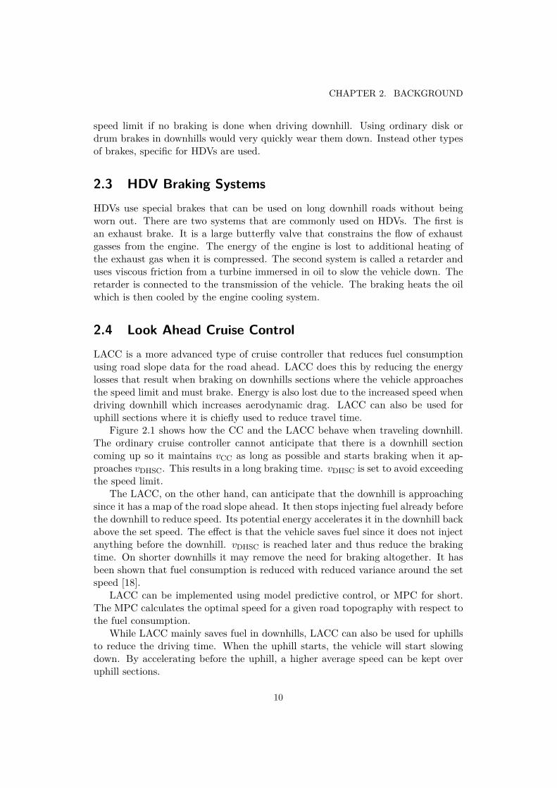
Figure 2.1 shows how the CC and the LACC behave when traveling downhill.The ordinary cruise controller cannot anticipate that there is a downhill sectioncoming up so it maintains vCC as long as possible and starts braking when it ap-proaches vDHSC. This results in a long braking time. vDHSC is set to avoid exceedingthe speed limit.
The LACC, on the other hand, can anticipate that the downhill is approachingsince it has a map of the road slope ahead. It then stops injecting fuel already beforethe downhill to reduce speed. Its potential energy accelerates it in the downhill backabove the set speed. The effect is that the vehicle saves fuel since it does not injectanything before the downhill. vDHSC is reached later and thus reduce the brakingtime. On shorter downhills it may remove the need for braking altogether. It hasbeen shown that fuel consumption is reduced with reduced variance around the setspeed [18].
LACC can be implemented using model predictive control, or MPC for short.The MPC calculates the optimal speed for a given road topography with respect tothe fuel consumption.
While LACC mainly saves fuel in downhills, LACC can also be used for uphillsto reduce the driving time. When the uphill starts, the vehicle will start slowingdown. By accelerating before the uphill, a higher average speed can be kept overuphill sections.
10
2.5. SENSORS AND DATA
Altitude
VCC
VDHSC
VMIN
Speed
VDHSC
VCC
Speed
Braking
Braking
Time
Figure 2.1. The speed profile that a look ahead cruise controller outputs, comparedto a standard cruise controller when driving in an idealized downhill. One can seethat the LACC reduces the speed of the vehicle already before the downhill and thusreduces the braking. The shape of the speed profiles is simplified in the figure.
2.5 Sensors and Data
An advantage of the considered prediction algorithms is that they do not need anymodifications to current hardware. All of the sensors needed will be available on amodern day production vehicle.
In order to predict the speed of the target vehicle, its speed and the currentroad slope must be known. The speed is determined from two sources. The relativespeed between the vehicles is determined using an automotive radar. The absolutespeed of the observing vehicle is determined using GPS and an inertial measurementunit (IMU). To determine the road slope for the target vehicle, a road slope map isneeded. The position of the target vehicle has to be known to read the road slopeat the correct location. The position is determined using the same sensors as thespeed.
2.5.1 Automotive Radar
Automotive radar is becoming a popular method of sensing for the purposes ofADAS. It is largely immune to adverse weather conditions, and has a large range,and good accuracy which makes it a more practical choice in many cases for simplerange measurements when compared to ultrasonic, machine vision or laser time-of-flight sensors. It is also relatively inexpensive.
11

CHAPTER 2. BACKGROUND
Automotive radar is essentially the same technology as is used in aerospace andmaritime applications. It transmits an electromagnetic signal which is then reflectedfrom conductive surfaces. To measure the distance to some target, the time of flightof the signal, from transmitted to reflected and received is used. When measuringmoving targets, the frequency of the transmitted and received signal will have aDoppler shift that can be used to determine the velocity of the target.
In this thesis we will not be concerned with computing these quantities as the au-tomotive radar sensor does so already and merely outputs the velocity and distanceto the target.
Currently, both automobiles and HDVs are being shipped with forward facingautomotive radar to measure the speed of the vehicle in front. The common use forthis is ACC and AEB.
2.5.2 Map DataHDVs are now frequently being supplied with road map data that includes the roadslope. The road slope data is a necessity for HDVs equipped with LACC and couldalso be used for the purposes of speed prediction.
2.5.3 IMU & GPSVehicles are being outfitted with more accurate means of localizing themselves foruse in ADAS. The GPS needs no introduction. A drawback of GPS is that it mayloose connection in tunnels or other areas with no line of sight to its satellites.
A complement to GPS in such situations is an inertial measurement unit (IMU).It consist of accelerometers that measure the acceleration of the vehicle in multipledirections. The accelerations are then integrated to obtain the speed and the po-sition of the vehicle. The two systems function as a whole to output an absolutespeed and position of the observing vehicle.
12

Chapter 3
Grey Box Model
Grey box models are system models that are based on the physical principles gov-erning the behavior of the system and that contain unknown parameters. The valuesof the physical parameters are found by fitting the grey box to data obtained fromthe system. For more information on building grey box models refer to [19].
Previous attempts at modeling the dynamics of HDVs have been focused on greybox modeling but there have been difficulties with this approach [7]. Despite this,it is decided to also begin with the grey box approach in order to gain insight intothe system and to understand why previous attempts encountered difficulties.
3.1 The Analytical Vehicle ModelThe dynamics of the HDV can be represented by an analytical model that takes intoaccount the main forces acting on the vehicle. Figure 3.1 illustrates these forces.The model is given by applying Newton’s second law. The model has been used inmany papers on platooning and HDV speed controllers [8, 9, 5, 6, 18]. Here, themodel will both be used to simulate HDV behavior and will also be used in attemptsto model the vehicle dynamics using a grey box model. The model has the form
ma = Fe − Fa − Fr − Fg, (3.1)
where Fe is the force produced by the engine, Fa is the force due to aerodynamicdrag, Fr is the rolling resistance force on the tires and Fg is the gravitational forcedue to the mass of the vehicle when traveling in a slope. In order to obtain a usefulmodel of the vehicle dynamics, the individual forces should be, as far as possible,expressed so that all time varying quantities are measurable.
3.1.1 Engine Force
The torque generated by the engine from fuel combustion results in a torque on thedriving wheels. To understand this relation, one can look at an idealized model ofan HDV drive train as shown in Figure 3.2. The drivetrain consists of six major
13

CHAPTER 3. GREY BOX MODEL
α
Fa
mg
Fe
Fr
Figure 3.1. An illustration of the forces acting on the vehicle when traveling on aninclined road.
TE' TE TC
1 2 3 4
5
TG
TFωwωGωCωE
6
Figure 3.2. A simplified illustration of an HDV drivetrain. 1. Engine; 2. Flywheel;3. Clutch; 4. Gearbox; 5. Final Drive; 6. Wheels.
components: 1, the engine; 2, the flywheel; 3, the clutch; 4, the transmission, 5, thefinal drive; and 6, the wheels.
A series of simplifying assumptions is made. The assumptions were found byothers to result in an accurate representation of the dynamics of an HDV whilereducing model complexity [7].
• The clutch is assumed to have no slip. That is, it is assumed that the torquesand the angular velocities on either side of the clutch are the same.
• The rotational inertia for most of the components in the drivetrain is ne-glected.
• The transmission is assumed to have a fixed gear ratio.
14

3.1. THE ANALYTICAL VEHICLE MODEL
S S TF TF S TF FPvFPTP
ωw
Tb
I:Jw
JwωwTG
ωwωGωCTGTCTE
ωE
ωE
ωETE'
I:JE
TE'1/rwɣFɣG
ηG ηFJEωE
Figure 3.3. Bond graph of the simplified drivetrain. The input is the engine forceand the output is the longitudinal force due that is produced on the wheels.
• The final drive is not assumed to have any differential, and is only seen asa fixed gear ratio. I.e., it does not permit the wheels to rotate at differentvelocities.
• The retarder and exhaust brake are omitted in order to simplify the model.The torques from the retarder will, falsely, be assumed to originate from theengine.
In order to structure the modeling of the drivetrain, the system is representedin bond graph form described in [19]. A bond graph for the drive train is shownin Figure 3.3. Note that Fe in (3.1) is represented by Fp in the bond graph toseparate it from the properties of the engine. Bond graphs simplify the modeling ofmulti-domain systems by recognizing that conservation of flow and conservation ofenergy laws are similar between domains. A complete introduction to bond graphmodeling can be found in [19].
The arrows, or bonds, represent power transfer and point from power sourcestoward sinks. Each bond has an effort and a flow variable. Here, torques and forcesare efforts, while rotational and linear velocities are flows. The ’S’ represents a seriesjunction, a junction where flow is the same for all bonds connected to it. The ’TF’symbol represents a transformer, a device that multiples the effort while dividingthe flow by the same amount. A real life example of a transformer is for example anelectrical transformer, a lever, or a transmission. Here the transmission, the finaldrive and the action of the wheels on the road can be represented as transformers.γG and γF represent the gear ratios of the transmission and the final drive. ηG
and ηF are their respective energy efficiencies. The ’I’ is used to represent an effortstorage, such as an inertia. There are two major inertias in the drivetrain: therotational inertia of the flywheel, Je, and the rotational inertia of the wheels, Jw.All the variables used in the drive train are described in Table 3.1.
Just like in classical mechanics, multiple transmissions, here as transformers,can be simplified into one where the gear ratio is the product of the gear ratios of
15

CHAPTER 3. GREY BOX MODEL
Table 3.1. The variables used in the drivetrain model.
TE′ Engine torque before without flywheelTE Engine torque with flywheelTC Torque on clutch outputTG Torque on gearbox outputTF Torque on final drive outputωE Angular velocity of engine outputωC Angular velocity of clutch outputωG Angular velocity of gearbox outputωW Angular velocity of wheelsJE Rotational inertia of flywheelJW Rotational inertia of wheelsγG Gearbox gear ratioγF Final drive gear ratioηG Gearbox efficiency coefficientηF Final drive efficiency coefficientv Vehicle speedrw Wheel radiusFp Propulsive force, same as Fe
S S TF S TF FPvFPTP
ωw
Tb
I:Jw
Jwωw
ωwωCTCTE
ωE
ωE
ωETE'
I:JE
TE'1/rwɣGɣF
ηGηFJEωE
Figure 3.4. Reduced bond graph of the drive train where the multiple transformerswere contracted into one.
the individual transmissions. The bond graph after this simplification is shown inFigure 3.4.
Combining the equations for all the junctions gives the following equation
Fp = γGγF ηGηF
rwTE′ − γ2
Gγ2F ηGηFJe
r2w
v − Jw
r2w
v. (3.2)
Inserting (3.2) into (3.1) and collecting all the inertia terms on the left handside
16

3.1. THE ANALYTICAL VEHICLE MODEL
mv = Fp − Fa − Fr − Fg, (3.3)(m+ Jw
r2w
+ γ2Gγ
2F ηGηFJe
r2w
)v = γGγF ηGηF
rwTE′ − Fa − Fr − Fg (3.4)
gives the equivalent inertia
mtot = m+ Jw
r2w
+ γ2Gγ
2F ηGηFJe
r2w
, (3.5)
where the first term is the mass of the vehicle, the second is the contribution fromthe wheel inertia and the third is the contribution from the flywheel inertia. Theforce equation then becomes
mtota = keTe − Fa − Fr − Fg, (3.6)
were the prime notation in the torque variable has been dropped and ke is given by
ke = γGγF ηGηF
rw. (3.7)
3.1.2 Aerodynamic Drag
A commonly used model of aerodynamic drag is
Fa = 12cdAaρav
2 = kav2, (3.8)
where cd is the drag coefficient, Aa is the frontal area of the vehicle and ρa is thedensity of air. In reality, the aerodynamic drag will also depend on any wind speeds,or if there are any vehicles driving in front of the modeled vehicle. These effects areomitted here.
3.1.3 Rolling Resistance
The rolling resistance is the force caused mainly by the friction between the wheelsand the road surface. An approximate model for this force is given by
Fr = crmg cos (α(s)) = kr cos (α(s)), (3.9)
where cr is the rolling friction coefficient, m is the vehicle mass, g is the gravitationalconstant and α(s) is the road angle that is a function of the position s along theroad.
17

CHAPTER 3. GREY BOX MODEL
3.1.4 Gravitational ForceWhen the vehicle is traveling on an inclined road, the gravitational force will havea component in the direction of vehicle motion. Since the vehicle mass for HDVs israther large, this force becomes large as well, even for moderately steep roads. Theforce is given by
Fg = mg sin (α(s)) = kg sin (α(s)). (3.10)
3.1.5 Combined ModelIncorporating all these force sub-models into (3.6) and using the combined constantske, ka, kr and kg results in
mtotv = keTe + kav2 + kr cos (α(s)) + kg sin (α(s)). (3.11)
The constantsmtot, ke, ka, kr and kg completely describe the dynamics of the vehiclefor known engine torque Te, speed v and road angle α. If one is able to identifythem, then the vehicle model is known.
3.2 Estimating Model CoefficientsA first attempt at estimating the model coefficients could be to simply use linearregression and fit the parameters with least squares. Linear regression problems areof the form
y = θTφ(t), (3.12)
where φ(t) is a vector of some known inputs, y is a known output and θ is a vectorof the unknown parameters. The vehicle model can be put in this form by dividingthe dynamics equation by the total inertia and setting y := a. The vehicle modelequation in the desired form is
y = 1mtot
(keTe − kav2 − kr cosα(s) − kg sinα(s)), (3.13)
where θ and φ(t) are given by
θ = 1mtot
(ke ka kr kg)T , (3.14)
φ(t) = (Te − v2 − cosα(s) − sinα(s))T . (3.15)
For more information on parameter estimation using linear regression, see [20].The speed and the acceleration for estimating the parameters can be determined
using the radar. The radar only outputs position and speed, but the accelerationcan be obtained by differentiating the speed numerically. The slope is obtainedfrom map data. The torque is more tricky to obtain. One needs a model of the
18

3.3. SIMULATING DATA
controller to determine it. A possible alternative is to await situations where thetorque is known, as it was done by Felixson [5]. These situations could be steepenough uphills where one can assume that the vehicle is using maximum torque.Also the torque is zero when the vehicle is coasting with the clutch disengaged.
3.3 Simulating Data
Simulation is a useful method of gaining intuition of how a system behaves. Itallows one to adjust parameters that are usually difficult to change when using reallife data. It also permits the modification of the system so that certain aspects ofit can be tested in isolation. Of course, simulating data instead of using real datacollected from test drives does not come without drawbacks. The most significantissue is that the simulation is based on a simplified model of the real thing and willnot exhibit some of the properties that the real life system may have.
Nonetheless, a simulation is chosen as a first step to obtain data from whichthe parameters of the grey box model can be estimated. The idea is that if knownparameters are used to generate the data, then the parameter estimation shouldreturn these within some margin of error that depends on the noise used to simulatethe radar measurement.
The real life situation involves both an observing vehicle and a target vehicle.In the simulation, only the motion of a single vehicle is modeled. It is assumed thatthere is no error in the map data compared to the real world slope. Moreover, itis assumed that the errors in the speed estimate that in the real life scenario comefrom errors of the observing vehicle’s IMU/GPS and the radar can be combinedinto a single error in the observation given by white Gaussian noise with zero mean.It is also assumed that the error in the speed from the radar is much greater thanfrom the GPS so that the error contribution from the latter can be neglected.
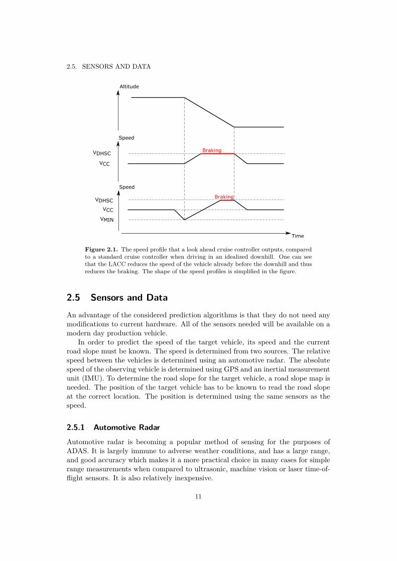
A simulation environment is created in Simulink. See Appendix A for anoverview of the simulation. The dynamics of the vehicle are represented using(3.11), the same equation of motion as the parameters are being fitted to. The pa-rameters were chosen as typical values for a long-haul HDV. The parameter valuesthat are used for the simulation are listed in Table 3.2.
The engine torque is controlled by two PID controllers. It can output torquesfrom 0 to 2500 Nm or it can coast, in which case the torque is -200 Nm. If thespeed of the vehicle exceeds vDHSC then another PID for the downhill speed controlcan apply a braking torque between -200 and -3000 Nm. This braking torque is,somewhat falsely, assumed to originate at the engine. If an exhaust brake is used,then the braking torque will indeed originate from the engine. A retarder on theother hand, will act on the transmission. A braking system would use both a enexhaust brake and a retarder to slow the vehicle down.
The PID controllers have rather large proportional gain, so that when combinedwith the saturation of the permitted engine and braking torques they operate sim-ilarly to a bang-bang controller. While this would be undesirable for a real engine
19
CHAPTER 3. GREY BOX MODEL
Table 3.2. The parameters used for simulating the vehicle speed when driven usingCC
vCC 80 km/hVDHSC 84 km/h
m 40000 kgγG 1γF 2.71ηG 0.97ηF 0.97rW 0.5 m
Te,max 2500 NmTe,min −200 Nm
Tbrake,max 3000 Nmcd 0.56Aa 10 m2
ρa 1.29 kg/m3
cr 0.007g 9.82 m/s2
Jw 32.9 kgm2
JE 3.5 kgm2
controller due to engine wear, it is acceptable for use on a simulated vehicle. Fig-ure 3.5 shows the simulated speed and torque of the vehicle using the parameters inTable 3.2. The initial ramp in the speed is due to the vehicle accelerating up to setspeed vCC from standstill. The set speed vCC is the speed that the cruise controllertries to maintain. The bottom plot shows the simulated torque output from thecontroller that exhibits bang-bang behavior.
The simulation assumes that the vehicle always drives in only one gear. Thegear ratio for this gear was chosen to be the highest gear in a real HDV. The inputto the simulation is the real road slope measured for the road from Södertälje toNorrköping.
3.4 Parameter Estimation Outcome
As an initial attempt at the parameter estimation problem, it is assumed that thetorque is known. First the data is generated using the simulation. The data is thenused to estimate the parameters offline. The same analytical model is used bothfor generating the data as is used for fitting the parameters. It should result in lowerrors as long as there is no noise. While this scenario is very distant from reality, itserves as a baseline test. The sampling period used is 0.5 s with a total data lengthtime of 1200 s.
20

3.4. PARAMETER ESTIMATION OUTCOME
0 200 400 600 800 1000 1200
Spee
d [m
/s]
0
5
10
15
20
25
0 200 400 600 800 1000 1200
Elev
atio
n [m
]
-20
-10
0
10
20
Time [s]0 200 400 600 800 1000 1200
Torq
ue [N
m]
-4000
-2000
0
2000
4000
Figure 3.5. The output of the cruise control and downhill speed control simulationusing the road slope data for the road from Södertalje to Norrköping. The initialslope is the vehicle accelerating up to CC speed in the highest gear.
3.4.1 Constant Torque, Open Loop, Noise Free
In this case, since there is no feedback controller, a constant torque of 2500 Nm isinput into the vehicle model. A constant input is a poor signal for system identi-fication since it does not excite multiple frequencies and amplitudes of the system.The reason for choosing constant maximum torque is that it is realistic to guessinstances when an HDV is applying maximum torque. The speed measurement bythe radar is assumed to be perfectly noiseless. Estimating the parameters usingleast squares results in the relative errors in Table 3.3. As expected, the errors arevery low since the same structure is used to both generate the data and estimatethe parameters. The only error in the parameters is due to finite precision in thenumeric calculations.
3.4.2 Constant Torque, Open Loop, Noisy
We now estimate the parameters in a similar simulation set up as above, where thetorque input is a constant 2500 Nm but where there is measurement noise. The
21

CHAPTER 3. GREY BOX MODEL
Table 3.3. Relative error in the estimated parameters for an open loop system withconstant input and no added measurement noise on the output.
Parameter ke ka kr kg
Relative Error 1 × 10⁻¹⁴ 1 × 10⁻¹⁵ 5 × 10⁻¹⁴ 1 × 10⁻¹⁵
Table 3.4. Relative error in the estimated parameters for an open loop system withconstant input and measurement noise on the output.
Parameter ke ka kr kg
Relative Error 1 0.1 6 0.005
Table 3.5. Relative error in the estimated parameters for a closed loop systemwithout measurement noise on the output.
Parameter ke ka kr kg
Relative Error 1 × 10⁻¹⁵ 4 × 10⁻¹⁴ 3 × 10⁻¹⁴ 1 × 10⁻¹⁵
speed measurement noise of the radar is approximated as white Gaussian noise withthe standard deviation chosen to match the accuracy of a common radar used in theautomotive industry. The standard deviation of the noise was set to 0.125 m/s. Toobtain the acceleration, the noisy speed signal is differentiated using the backwardEuler method.
The relative errors can be seen in Table 3.4. Even with this heavily idealizedscenario, where the system is open loop with only some measurement noise, the errorin the rolling resistance is up at 600% of the reference value. One can expect thedifferentiation of the noisy speed signal to result in an even more noisy accelerationsignal.
3.4.3 Cruise Control, Closed Loop, Noise Free
The next step is to close the loop and let the CC algorithm regulate the speed ofthe vehicle. The observed speed from the radar has no noise, but it is differentiatedto yield acceleration as before. The relative errors of the parameters are listed inTable 3.5. Again, the errors are at the precision of the numeric calculations.
3.4.4 Cruise Control, Closed Loop, Noisy
Now the closed loop system has the same measurement noise added to it as in thecase of the open loop system. The parameter errors are presented in Table 3.6. Theresult is large errors in the air drag coefficient and the rolling resistance coefficient.
3.4.5 Other Tests
Experiments were done to reduce the problems with differentiation of the noisyspeed signal in closed loop estimation. An attempt was made to smooth the noisy
22

3.5. PREDICTION BY SIMULATION
Table 3.6. Relative error in the estimated parameters for a closed loop system withmeasurement noise on the output.
Parameter ke ka kr kg
Relative Error 1 54 33 1
speed prior to numerical differentiation. Also, another attempt was made to avid ex-plicit differentiation by representing the vehicle dynamics represented in state spaceform and estimating the parameters using prediction error minimization. Neitherof these approaches resulted in any significant improvements. Attempts were alsomade to simultaneously evaluate the coefficients of a basic controller. Doing sogreatly increased the error in vehicle model parameters.
3.5 Prediction by SimulationThe goal of the parameter prediction is not to find the parameters in themselves, aswas done in previous research, but instead to predict the speed profile. To do this,the estimated parameters are inserted back into the vehicle model and the speedprofile for a given road slope is simulated.
The most realistic case of closed loop estimation with measurement noise couldnot be simulated due the large parameter errors. The errors in the parameters madethe vehicle drive backwards and since the road slope data is only defined for positivedistances, the simulation failed.
The open loop simulation could be simulated and the simulation output is shownin Figure 3.6. Even in this unrealistic case the parameter estimation results in poorprediction accuracy.
3.6 Grey Box Modeling SummaryThe brief experimentation in Sections 3.4 to 3.5 shows multiple limitations of greybox model estimation methods for the considered application. Closing the loopincreased the errors to such extent that it is no longer possible simulate the speedof the vehicle. A difficulty that closed loop identification generally poses is thatthe output amplitude is limited by the controller. It is possible that the cause ofincrease in the parameter errors is due to insufficient amplitude variation of theinput. The parameters with the largest errors for the closed loop case, air drag androlling resistance, corresponded to the terms with the lowest forces. The correlationbetween the different force terms is another issue. The air drag term is close toconstant since the speed is close to constant at vCC with only small deviationsabove and below it. The rolling friction term contains the factor cos(α(s)) whereα(s) ≈ 0 and therefore cos(α(s)) ≈ 1. This means that the contributions from thesetwo terms are very difficult to separate in order to estimate their coefficient values.The engine and gravity terms also have a problem with correlation. The CC will
23

CHAPTER 3. GREY BOX MODEL
100 200 300 400 500 600 700 800 900 1000 1100 1200
Spee
d [m
/s]
10
20
30
40
50
60
PredictionReference
Time [s]100 200 300 400 500 600 700 800 900 1000 1100 1200
Elev
atio
n [m
]
-30
-20
-10
0
10
20
30
Figure 3.6. The top plot shows the predicted speed for the open loop system whenthe constant maximum torque is applied along with the reference speed with thecorrect parameter values. The bottom plot shows the road angle for the predictedspeed.
increase Te whenever α increases leading to correlation between the terms. Furtherinvestigations into the causes of the errors are not made as the grey box approachis deemed impractical due to the necessity of of knowing the engine torque.
The experiments performed here have their limitations. The simulation thatwas used may not be representative of real world CC controllers. The scenario ofconstant maximum torque results in unrealistic speeds giving excessive aerodynamicdrag. It cannot be excluded that some of the issues encountered with grey boxmodeling are due to unrealistic testing.
24
Chapter 4
Black Box Modeling
As a result of the problems with the grey box modeling approach, black box mod-eling of the speed profile is attempted. Black box modeling gets its name from thatthe system is seen as a black box with unknown internals but with known inputsand outputs. One does not attempt to understand the inner workings of the systemand build a model based on it. Instead, one tries to reliably predict the outputs ofthe system given its inputs.
Already at the start, black box modeling has a series of advantages over param-eter estimation in physically motivated grey box models. The vehicle model doesnot need to be known, nor do the exact workings of the controller. The enginetorque does not need to be known or estimated.
The background theory for the various structures of black box models is de-scribed here only very briefly. For a more elaborated description of ARX, ARMAX,BJ and nonlinear ARX models see [20].
4.1 ARX Model
There are numerous black box model structures used in system identification. One ofthe most common is the Auto Regressive eXogenous model or ARX model structure.It models the future outputs as a linear function of weighted past inputs and outputs.
ARX models have the advantage that they can be solved using least squares inclosed form. Many more complicated model structures must have their parametersestimated using an iterative method to minimize the prediction errors.
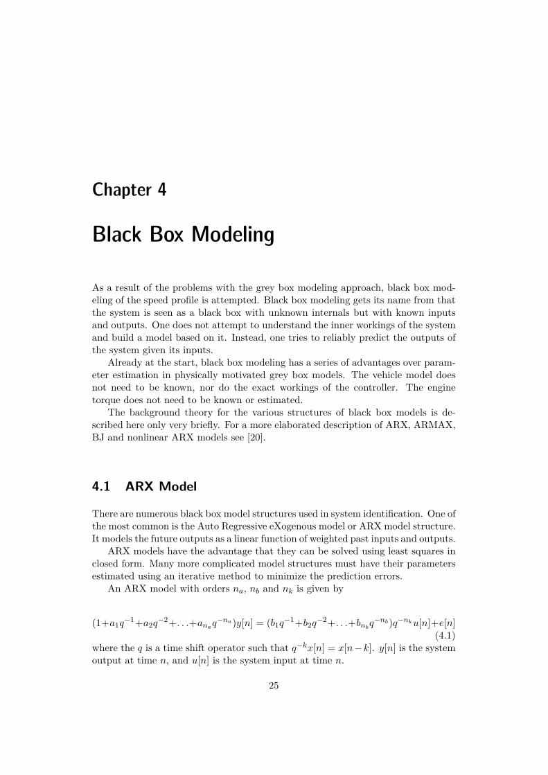
An ARX model with orders na, nb and nk is given by
(1+a1q−1+a2q
−2+. . .+anaq−na)y[n] = (b1q
−1+b2q−2+. . .+bnb
q−nb)q−nku[n]+e[n](4.1)
where the q is a time shift operator such that q−kx[n] = x[n−k]. y[n] is the systemoutput at time n, and u[n] is the system input at time n.
25

CHAPTER 4. BLACK BOX MODELING
4.2 Box-Jenkins ModelA common, more adaptable model structure is a Box-Jenkins model structure. Itis nonlinear in its parameters and must be estimated using an iterative method forprediction error minimization. It is given by
y[n] = B(q)F (q)u[n] + C(q)
D(q)e[n] (4.2)
with B(q), F (q), C(q), D(q) being polynomials in the time delay operator q withorders nb, nf , nc, nd respectively. B(q) is given by
B(q) = b1q−1 + . . .+ bnb
q−nb (4.3)
while the remaining expressions, F (q), C(q) and D(q) are polynomials of the form
F (q) = 1 + f1q−1 + . . .+ fnf
q−nf , (4.4)
where the first term is equal to 1.
4.3 Nonlinear ARX modelsNonlinear ARX or NARX is a large family of black box models with the genericform
y[n] = g(u[n− nb − nk], . . . , u[n− nk], y[n− na], . . . , y[n− 1]), (4.5)
where g is a nonlinear function of the regressors u[n − nb − nk] ... y[n − 1]. Thenonlinear function can be one of very many types: examples include networks ofsigmoid functions or wavelets.
4.4 Assessing FitTo be able to compare different black box estimates one has to assess their accuracy.A common measure of the accuracy is the root mean square error or RMSE
RMSE(y) =√E[(y − y)2]. (4.6)
It has the drawback that it cannot be used to compare the accuracy of modelsbeing used on different datasets since it varies with the magnitude of the data inthe dataset. A measure that is more comparable between datasets is the normalizedroot mean squared error. It is normalized with respect to the error when estimatingusing the mean:
NRMSE(y) = 1 −√E[(y − y)2]√
E[(E[y] − y)2]. (4.7)
26

4.5. CC MODELING
100 200 300 400 500 600 700 800 900 1000 1100 1200
Spe
ed [m
/s]
-4
-2
0
2
testing training
Time [s]100 200 300 400 500 600 700 800 900 1000 1100 1200
Roa
d A
ngle
[rad
]
-0.06
-0.04
-0.02
0
0.02
testing training
Figure 4.1. The simulation data used for black box modeling of CC. The data forthe training of the model and the data for testing the trained model are shown indifferent colors. The means have been removed from the data.
4.5 CC Modeling
4.5.1 Black Box Models on Simulated Data
The black box modeling is initially attempted on the data from the CC simulationdescribed in Section 3.3. The initial acceleration is removed from the data. It isthen split into training data and validation data. The training data is selected toinclude some large deviations from the set speed vCC. Unfortunately, road sectionsthat are sufficiently steep for the speed to deviate from the set speed do not occurvery often. This is representative of real life where it will not be possible to collectdata with many large excitations before having to predict the speed. The data usedfor the black box modeling is shown in Figure 4.1.
ARX, BJ and NARX models were fitted to the training data. Figure 4.2 com-pares the outputs of the models to the validation data. Only the model order thatwas found to give the best prediction accuracy for each model structure is plotted.The fit of the models is evaluated using NRMSE. The fit of the ARX model withna = 4, nb = 4 and nk = 1 (arx441) model is 39 % . The fit of the BJ modelwith nb = 2, nc = 2, nd = 2, nf = 2 and nk = 1 (bj22221) is 42 %. While theBox-Jenkins model gives slightly better accuracy on the validation data, both arerather poor. The Box-Jenkins model has much greater complexity yet it does not
27

CHAPTER 4. BLACK BOX MODELING
Time [s]500 600 700 800 900 1000 1100 1200
Spee
d [m
/s]
-2.5
-2
-1.5
-1
-0.5
0
0.5
1
1.5
nlarxbj22221arx441Reference
Figure 4.2. The outputs of an ARX, BJ and an NARX model compared to thesimulated speed.
improve performance significantly. The NARX was a wavelet network with 4 unitsfrom the System Identification Toolbox in MATLAB. The chosen regressor orderswere na = 2 nb = 2 nk = 1. It had the best accuracy at 46 % but was by far themost complex. The hope was that a nonlinear model would be best at describingsuch a highly non-linear system yet it did not cope well with predicting the sectionsthat do not deviate significantly from the set speed.
The non-linearity of the controller is most likely the main obstacle to obtain agood fit for the system. While it is difficult to show formally, angles below somethreshold result in next to no offset from the set speed, while road angles that exceedthis threshold result in quite large deviations from the set speed. This should becharacteristic for all CC controllers. The predictions do not mimic this behaviorand have almost equally large deviations for all road sections. A limitation of usingthe simulated data is that the controller is not a real controller that is used in HDVsbut a rather simplistic attempt of emulating one.
4.5.2 Black Box Models on Real Life Data
To evaluate if black box modeling is a reasonable approach for predicting vehiclespeed, real life data collected during an HDV drive was used. The data was selectedso that the cruise controller was engaged during the entire data set. Figure 4.3 showsthe measured real life data. The training data was selected so that it includes asteep downhill and uphill.
One can see that the real life controller is not as strict as the simulated one.Also, the upper limiting speed for the downhill speed control, vDHSC, is set higherthan what was used in the simulation. The action of the DHSC is therefore notas noticeable, The offset from the set speed is much larger for the fairly flat road
28

4.6. LACC MODELING
0 200 400 600 800 1000 1200 1400 1600 1800
Spe
ed [m
/s]
-2
0
2
4
6
testing training
Time [s]0 200 400 600 800 1000 1200 1400 1600 1800
Roa
d A
ngle
[rad
]
-0.05
0
0.05
0.1
testing training
Figure 4.3. The real life data that was used for black box prediction of the speed.
sections than for the simulated data, which is favorable when modeling.Figure 4.4, shows the results of fitting the models to the real life data. The
same ARX, BJ and NARX models are used. Increasing model order did not resultin any significant improvement in the accuracy in predicting the validation data.The NRMSE of the fit of the prediction was 31 %, 34 % and 39 % for the ARX, BJand NARX respectively. The non-linear model did result in an improvement butincreasing its complexity did not improve the fit.
4.6 LACC ModelingCompared to gray box modeling, black box modeling showed produced useful re-sults on CC data without assuming anything about the controller or the vehicle.Black box modeling seems therefore like a good starting point for LACC modeling.Unfortunately, LACC speed profiles are not equally correlated with the road angleas the CC speed profiles. Correlation between the vehicle speed and the road angleare calculated using
r =∑N
i=1(vi − v)(αi − α)√∑Ni=1(vi − v)
√∑Ni=1(αi − α)
, (4.8)
where N is the number of samples in the dataset. The correlation between thespeed and the angle for the CC was 0.7. On the other hand the same correlationmeasurement for the LACC dataset showed a correlation of -0.3.
29

CHAPTER 4. BLACK BOX MODELING
Time [s]800 900 1000 1100 1200 1300 1400 1500 1600 1700 1800
Spe
ed [m
/s]
-2
-1
0
1
2
3
4
5
nlarxbj22221arx441Reference
Figure 4.4. The outputs of an ARX a BJ and a NARX model compared to thereference speed. The data set is shown in Figure 4.3.
A large part of the challenge in estimating the LACC profiles lies in the timingof the initial speed drop. The timing depends not only on the topographic profileof the road but also on the unknown parameters of the target vehicle. The systemacts noncausally in terms of the input, the road angle, and the output, the speedprofile. Generally, autoregressive black box models can only account for positivedelays in the output, not negative, as the delays are in the case of LACC.
A series of black box models were fitted to the LACC data to see how theyperform. The result is shown in Figure 4.5. The same two models that were usedfor the CC black box modeling were also used here. Increasing the model order foreither model did not improve accuracy significantly. It can be seen in Figure 4.5that the speed dips at the start of a LACC speed profile for a downhill are modeledvery poorly, or not modeled at all. The speed dips at the start of a LACC speedprofile can be recognized by that they directly precede a speed peak.
To help with modeling the speed dips from the downhills, the road angle datawas shifted backwards relative to the speed so that the downhills started before thespeed dip. This is supposed to result in a positive delay. A problem that arisesinstead is that the speed when not in a LACC curve has a significant delay thatmakes modeling of these parts more difficult.
NARX models should cope better with the nonlinear nature of the speed profiles.The outputs of the most accurate NARX model obtained is shown in Figure 4.6.This model achieves an accuracy of 64 %. Here the verification and the trainingdata sets are the same so overfitting is a big concern. There is insufficient data tosplit the data in half and still have the NARX model fitting converge. The fittingconverges when the model is trained on all the data except the three last LACCprofiles. Figure 4.7 shows the output of two NARX models for the last three LACCprofiles. The greatest fit is 44 % and looking at Figure 4.7, it can be seen that thegeneral trends are modeled, although not very accurately. The model used was a
30

4.6. LACC MODELING
Time [s]0 500 1000 1500 2000 2500 3000 3500 4000 4500 5000 5500
Spe
ed [m
/s]
-15
-10
-5
0
5
arx441 bj22221 Reference
Figure 4.5. An ARX and a BJ model output compared to the reference speed. Thereference data is part of a simulated data set.
Time [s]0 1000 2000 3000 4000 5000 6000
Spe
ed [m
/s]
-5
-4
-3
-2
-1
0
1
2
3
nlarx Reference
Figure 4.6. The output of the best NARX model is compared to the reference speed.The reference data is part of a simulated data set. The same data is used for bothverification and training.
sigmoidal function neural network with 10 units with orders na = 10, nb = 20 andnk = 1. The data is decimated to a relatively low sampling time so that the blackbox models do not need to have hundreds of regression terms.
NARX modeling improved the modeling of the speed drops in the LACC profiles.NARX models have their own problems that unfortunately make them impracticalfor online speed prediction. They require a lot of data, or the numerical solver usedto fit the model will not converge to any stable solution. One would need to followthe same vehicle for a very long time to collect sufficient data to be able to train aNARX model.
31

CHAPTER 4. BLACK BOX MODELING
Time [s]4700 4800 4900 5000 5100 5200 5300 5400 5500
Spee
d [m
/s]
-5
-4
-3
-2
-1
0
1
2
3
nlarxReference
Figure 4.7. Plot comparing NARX model trained on 4700 s of LACC data to thereference speed. The reference speed is part of is from a simulated LACC datasetusing a Scania simulation environment.
4.7 Black Box Modeling SummaryBlack box modeling has some significant advantages over grey box modeling. Thenoise in the speed is less of a concern since it is not necessary to have the accelerationand differentiate the speed. Unlike simulating with parameters, a separate modelof the unknown controller is not needed. The drawback of the simpler black boxmodels is that they have difficulties capturing the nonlinear behavior of the system.More advanced models, on the other hand, need large amounts of data and areimpractical for use in real time vehicle speed prediction.
32

Chapter 5
Ad Hoc Models
The main difficulty encountered when trying to model the system using black boxmodels was that the linear models did not deal very well with the non-linear switch-ing behavior of the controller. The non-linear models were able to model this switch-ing better but required much more training data. One method of getting aroundthe problems of the switching behavior is to model the switching explicitly.
An approach is to separate the dynamics of the vehicle when traveling uphill,downhill and on level roads. This division is based upon general knowledge of HDVcontroller behavior. For sufficiently steep uphills, an HDV will apply maximumengine torque so the controller output is known. Similarly, for downhills, HDVs willbe coasting so the controller is also known. In the case of level road, the torque willvary, but the speed will not deviate significantly from the reference speed.
Let us use more exact definitions for what an uphill, a downhill and level groundare in the context of HDV speed.
• Uphill - The road is sufficiently steep so that the maximum engine torque isinsufficient to prevent the vehicle from slowing down from its set speed.
• Downhill - The road is sufficiently steep so that the energy losses whencoasting are insufficient to prevent it from accelerating.
• Level Road - The road is sufficiently flat so that the energy losses whencoasting are sufficient to keep it from accelerating and the maximum enginetorque is sufficient to keep it from slowing down.
There is an additional caveat for the downhill case. If the vehicle accelerates upto vDHSC traversing a downhill section, the DHSC brake systems will be engaged.The torque on the wheels is unknown in that case as well, but the speed should notdeviate significantly from the reference speed, vDHSC, of the DHSC system. Referback to Figure 2.1 for a reminder of how the DHSC works.
Two different types of switched ad hoc models have been tried. Both of themrely on identifying uphills, downhills and level road based on the road angle. Whatsets them apart is how the dynamics of the vehicle are modeled in the uphills and
33
CHAPTER 5. AD HOC MODELS
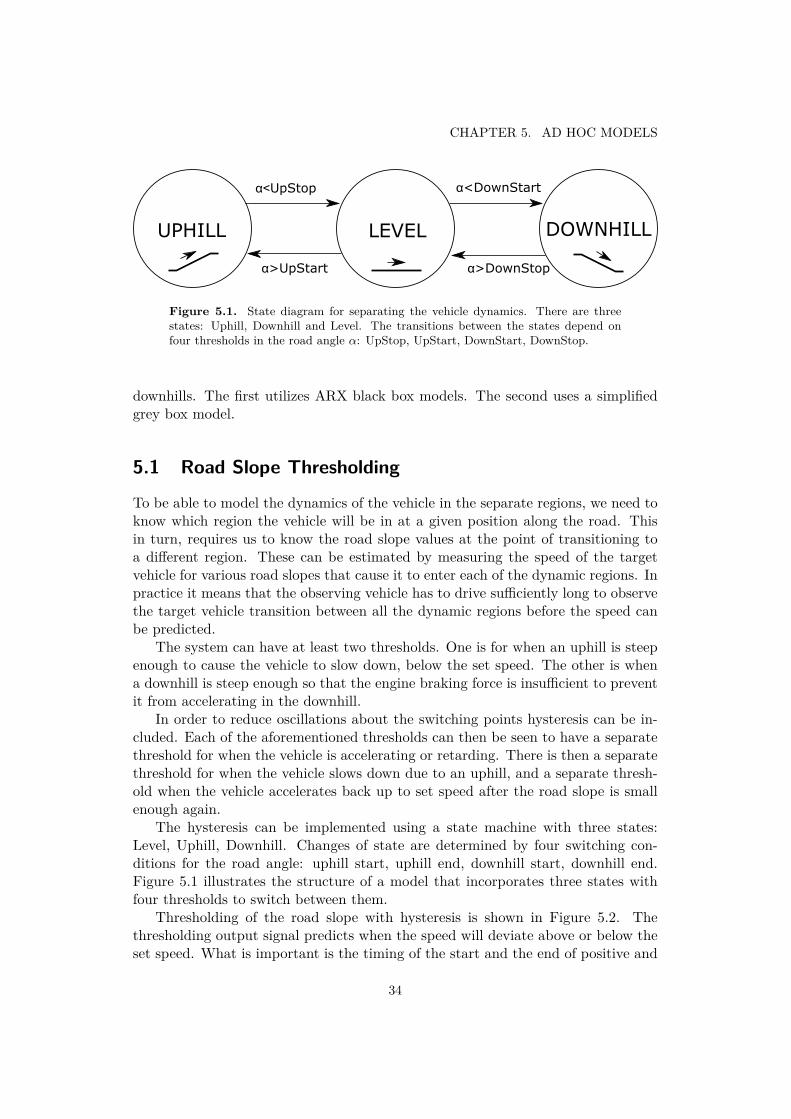
LEVEL DOWNHILLUPHILL
α>DownStop
α<DownStart α<UpStop
α>UpStart
Figure 5.1. State diagram for separating the vehicle dynamics. There are threestates: Uphill, Downhill and Level. The transitions between the states depend onfour thresholds in the road angle α: UpStop, UpStart, DownStart, DownStop.
downhills. The first utilizes ARX black box models. The second uses a simplifiedgrey box model.
5.1 Road Slope Thresholding
To be able to model the dynamics of the vehicle in the separate regions, we need toknow which region the vehicle will be in at a given position along the road. Thisin turn, requires us to know the road slope values at the point of transitioning toa different region. These can be estimated by measuring the speed of the targetvehicle for various road slopes that cause it to enter each of the dynamic regions. Inpractice it means that the observing vehicle has to drive sufficiently long to observethe target vehicle transition between all the dynamic regions before the speed canbe predicted.
The system can have at least two thresholds. One is for when an uphill is steepenough to cause the vehicle to slow down, below the set speed. The other is whena downhill is steep enough so that the engine braking force is insufficient to preventit from accelerating in the downhill.
In order to reduce oscillations about the switching points hysteresis can be in-cluded. Each of the aforementioned thresholds can then be seen to have a separatethreshold for when the vehicle is accelerating or retarding. There is then a separatethreshold for when the vehicle slows down due to an uphill, and a separate thresh-old when the vehicle accelerates back up to set speed after the road slope is smallenough again.
The hysteresis can be implemented using a state machine with three states:Level, Uphill, Downhill. Changes of state are determined by four switching con-ditions for the road angle: uphill start, uphill end, downhill start, downhill end.Figure 5.1 illustrates the structure of a model that incorporates three states withfour thresholds to switch between them.
Thresholding of the road slope with hysteresis is shown in Figure 5.2. Thethresholding output signal predicts when the speed will deviate above or below theset speed. What is important is the timing of the start and the end of positive and
34

5.2. CC MODELING WITH SWITCHED BLACK BOX MODELS
0 500 1000 1500 2000 2500
Spe
ed [m
/s]
17
18
19
20
21
Thresholding OuputActual Speed
Sample Number (sampled at 2 Hz)0 500 1000 1500 2000 2500
Roa
d A
ngle
[rad
]
-0.04
-0.02
0
0.02
0.04
Road AngleUphill StartUphill EndDownhill StartDownhill End
Figure 5.2. The upper figure shows the output of thresholding the road angle com-pared to the speed held by the vehicle. Note that the amplitude of the thresholdingoutput signal is arbitrary. It only indicates when the speed will deviate above orbelow the set speed.
negative offsets from the set speed. These occur at time points when the road slopepasses one of the thresholds or switching points as one can also call them.
In Figure 5.2, the switching conditions are chosen by averaging the slope whichresults in a speed offset that exceeds 1 km/h. The same data that was used todetermine the thresholds is also is used as verification in the plot. The plot showsthat a single set of switching points fits all the uphill and downhill speed offsetsrather well. By estimating these switching points it is possible to predict when thevehicle will accelerate or slow down due to road topography.
5.2 CC Modeling with Switched Black Box Models
The switched black box model is a natural progression from ordinary black boxmodeling. It uses two separate black box models, one for uphills and another onefor the downhills. It uses road slope thresholding to choose which model should beused. Due to the low pass character of ARX models, switching jitter between thestates is not a big issue and there is no need to use hysteresis thresholds. Only oneangle threshold for uphills and one angle threshold for downhills is used.
The general structure of the switched black box predictor is shown in Figure 5.3.The speed of the target vehicle is measured and stored. The road slope at the timescorresponding to the speed samples is obtained from map data. The first step is
35

CHAPTER 5. AD HOC MODELS
Set speed estimation
Flat road thresholding(Assuming conservative truck parameters)Road slope data
Speed from radar
Mean
Variance
Downhill datathresholding
Uphill datathresholding
ARX modelestimation
ARX modelestimation
Output simulation
Outputsimulation +
Prediction
Figure 5.3. An illustration of the structure of the switched black box model pre-dictor. The lines between the blocks represent information dependencies between theblocks.
then to estimate the cruise control set speed, vCC, of the target vehicle. When thespeed rises above or drops below the typical variance about the set speed, then thevehicle is assumed to be transitioning to either a downhill or an uphill. The roadslopes at those instances are used for selecting the training and prediction data forthe ARX black box models. The models are estimated and used to simulate thespeed for the road ahead. Finally, the set speed estimate and the uphill and downhillmodels outputs are added to yield the speed prediction for the target vehicle.
5.2.1 Set Speed Estimation
For the case when the target vehicle is driving on level ground, it is assumed thatthe controller maintains the speed of the vehicle close to the CC set speed, vCC.The CC set speed can then be used as the estimate of the speed on level road.The set speed has to be estimated from observing the target vehicle’s speed. Thereare a couple of possible approaches, for example, one could take the average of allobserved speeds. A problem with averaging all observed speeds is that it relies onthe unreliable assumption that the topography is near flat on average. If there ismore downhill driving than uphill driving, then the set speed will be overestimated.
The chosen solution is to only take the average of the speed when the targetvehicle is on level road. A drawback is that one does not have any estimate untilthe target vehicle has been observed driving on level road. To do this, one needs tohave a range of road angles that can be considered "level road" for most HDVs.
To calculate this range of road angles one can look at (3.1) again. It describesthe vehicle dynamics. There are two distinct limit cases: when the acceleration iszero and the vehicle is coasting traveling downhill, when the acceleration is zeroand the vehicle is using maximum torque traveling uphill.
The vehicle’s equation of motion (3.1), can be solved for the road angle. In bothlimit cases the acceleration is zero. The equation of motion therefore becomes
36

5.2. CC MODELING WITH SWITCHED BLACK BOX MODELS
mtota = Fe − Fa − Fr − Fg, (5.1)0 = keTe − kav
2 − kr cosα(s) − kg sinα(s). (5.2)
Using the small angle approximation, the sine is approximated by α(s) andcosine is approximated by 1. The equation is then solved for the road angle α(s),giving
α(s) = keTe − kav2cc − kr
kg. (5.3)
The values of the parameters ke Te ka vcc kr kg depend on which of the two casesis being considered. In either case the parameters should be chosen to result in aconservative estimate of the threshold angle. The road angles should be estimatedclose to zero so that one can be confident that most HDVs will be able to maintainCC set speed for these angles.
Case 1: Coasting in DownhillThe acceleration is zero, the vehicle is just barely managing to maintain constantspeed in the downhill by coasting, i.e., not injecting any fuel. The parameters arechosen so that the angle in (5.3) is as close to zero as is reasonable for a roadlegal HDV. The motor braking force is chosen to a low value of -150 Nm. Thevehicle mass on the other hand is chosen to be the largest legally permitted massin Sweden, 60 tons. It is one of the highest mass limits internationally. The speedof the vehicle is assumed to be 70 km/h so that the braking help from aerodynamicdrag is reduced. Other parameters are set to typical values, shown in Table 5.1.
Inputting the parameters into (5.3), the resulting road angle is
αdown = −0.0106 rad. (5.4)
Case 2: Maximum Torque in UphillIn the case of an uphill the acceleration is zero and the vehicle just barely managesto maintain constant speed by applying maximum torque. Again, the parametersare chosen to give an angle close to zero. The maximum engine torque is assumedto be a fairly low value of 1800 Nm. The speed is chosen as the Swedish speed limitof 90 km/h to increase drag. The mentioned parameters are listed in Table 5.2.The remaining parameters are the same as in Table 5.1.
The resulting road angle is
αup = 0.0047 rad. (5.5)
The slope interval for calculating the set speed is therefore αdown < αCC < αup.The speeds observed when the target vehicle is traveling on road sections that are
37

CHAPTER 5. AD HOC MODELS
Table 5.1. The parameters used for determining the road angle threshold for thecase of motor braking in a downhill.
vCC 70 km/hm 60000 kgγG 1γF 2.71ηG 0.97ηF 0.97rW 0.5 mTe −150 Nmcd 0.56Aa 10 m2
ρa 1.29 kg/m3
cR 0.007g 9.82 m/s2
Jw 32.9 kgm2
JE 3.5 kgm2
Table 5.2. The parameters used for determining the threshold for the case of max-imum torque in an uphill. The remaining parameters are the same as in table 5.1.
vCC 90 km/hm 60000 kgTe 1800 Nm
in this interval are averaged to produce the estimate of the set speed. The varianceabout the set speed is calculated by taking the sample variance for the speedsobserved when the target vehicle is on road with road slope in the mentioned range.
The pseudocode for the calculating the CC set speed is the following:
Let vseen be the vector of all observed speeds and αseen be the vector of thecorresponding road angles.
Put all vi,seen for which αdown < αi,seen < αup into set Vthresholded
Then the CC set speed is
vCC = E[Vthresholded],
and its standard deviation is
σCC = std(Vthresholded).
The standard deviation is used to determine the speed threshold at which one canidentify uphills and downhills. Section 5.2.3 elaborates on this.
38
5.2. CC MODELING WITH SWITCHED BLACK BOX MODELS
5.2.2 DHSC Modeling
The simplest estimate of the DHSC set speed, vDHSC, is the maximum observedspeed of the target. This estimate will deviate from the set speed by the controlerror of the DHSC. The predicted speed can then simply be saturated at vDHSC asa final step.
A more elegant solution would be to treat the DHSC as a separate state but doingso creates a number of problems. One of the main problems is how to separatelymodel just the rising and falling edges of the speed offset resulting from a downhill.
5.2.3 Modeling of Uphill and Downhill Dynamics
In order to know when to use which ARX model, the road angle thresholds needto be determined. The road angle for the transition to the downhill state, can beobserved when the speed exceeds the typical values for level road. This is wherethe standard deviation of the speed on level ground, σCC , comes into use. The roadangles corresponding to speed crossings a number of standard deviations abovevCC and at the end of DHSC are stored and averaged. Figure 5.4 shows how theroad angle threshold, called αd in the figure, is determined for downhills. The speedthreshold, v1, is chosen as a multiple of the σCC above vCC. The reason for choosingv1 slightly above vCC is to avoid registering false downhill starting points due tothe target vehicle’s natural tracking error around vCC. The slope at the transitionpoint, labeled 1 in Figure 5.4, is then used to determine αd. Transition point 2 canalso be used but is more difficult to detect. In reality, the two points will not occurat exactly the same road slope, partly due to the nonzero v1, and due to that theaerodynamic drag is different. The road angle for the transition to the uphill stateis determined similarly. The difference is that the points where the speed crossesby a number of standard deviations below vCC are used.
The training data is separated into uphill and downhill training data so thattwo different ARX models can be trained. The determined transition road anglesare used for this. The training data consists of the model input, the road angledata, and the model output, the speed. The output data for the downhill modelsis obtained by subtracting the set speed and then setting all the negative observedspeeds to zero. This leaves only the downhill training data. To obtain the trainingdata for uphills, the positive speeds are set to zero. The input data for uphillsis obtained by transforming the road angle so that the all road angles above thedownhill threshold angle are zero in the case of the downhill model. The inputdata used for simulating the output from the uphill and downhill ARX models istransformed identically.
Black box models were fitted to the downhill and uphill training data. Figure 5.5shows the data for positive offsets, i.e. downhills. Two black box models are fittedto the data. As previously, the Box Jenkins model has somewhat better accuracyat the cost of a much more complex model compared to the ARX. The quality of fitfor the bj22221 is 66 % while for the arx441 it is 59 %. Figure 5.6 shows the data
39

CHAPTER 5. AD HOC MODELS
t
tα
v
αd
vCCv1
1 2
Figure 5.4. An illustration of how the threshold angle for the transition to thedownhill state is determined. The upper top plot show the speed of the target vehicle.The bottom plot shows the corresponding road angle. The speed v1 is chosen basedon σCC . The road angles for points 1 and 2 generally will not coincide.
Time [s]
100 200 300 400 500 600 700 800 900 1000 1100
Off
se
t S
pe
ed
[m
/s]
0
0.5
1
1.5
2
bj22221
arx441
Reference
Figure 5.5. The predicted speed for the downhills. Two different black box modelsare used, an ARX model and a BJ model.
for the negative offsets, i.e. the uphills. This time the accuracy of both models isvery close. The accuracy of the bj22221 is 70 % while for the arx441 it is 69%. Thetests are performed on the data presented in Figure 4.1, with the first uphill anddownhill being used as training data.
The accuracy figures are somewhat misleading since the output is largely zero.One can see that the downhills have a poorer fit. The downhills are more difficultto estimate since they still contain non-linear behavior in the form of the DHSCbraking that saturates the signal. It would be preferable to just estimate the edgesof the model, but it is difficult to do. The uphills, on the other hand are fairlystraightforward to estimate since the system behaves approximately linearly in that
40

5.2. CC MODELING WITH SWITCHED BLACK BOX MODELS
Time [s]100 200 300 400 500 600 700 800 900 1000 1100
Offs
et S
peed
[m/s
]
-2.5
-2
-1.5
-1
-0.5
0
0.5
arx441bj22221Reference
Figure 5.6. The predicted speed for the uphills. Two different black box models areused, an ARX model and a BJ model.
case. The ARX model is what is used in the end, since it is simpler to estimatethan the Box-Jenkins and the difference in accuracy is negligible.
5.2.4 Combining the Models
Combing the models is a matter of adding the outputs of the models for uphillsand downhills with the CC set speed estimate. Figure 5.7 shows the predictedspeed using the switched ARX model method on a simulated data set. The dataand its division between training and testing data sets is the same as shown inFigure 4.1. The RMSE is 0.20 m/s and the NRMSE is 63 % for the version withoutthe DHSC modeling. For the version with DHSC modeling, the RMSE is 0.14 m/sand the NRMSE is 73 %. This can be compared to the best accuracy obtained inSection 4.5.1 on the same data set using black box modeling, which was 46 %.
5.2.5 CC Predictor Testing
The switched ARX predictor works much better than any of the ordinary black boxmodels on simulated data. The next step is to compare it on a real life data set.The same data as presented in Figure 4.3 is used along with the same division intotraining and testing data sets. The resulting prediction using the switched ARXmodel method is shown in Figure 5.8. The RMSE is 0.13 m/s and the NRMSE is57 %. The NRMSE can be compared to black box modeling in Section 4.5.2 which,in the best case, had an accuracy of 39 %.
5.2.6 Summary
The behavior of the CC for a target vehicle is found to be separable into fourregions of operation: flat, uphill, downhill and DHSC. The tree first regions aredefined by their road angle intervals. The DHSC is dependent on the predicted
41
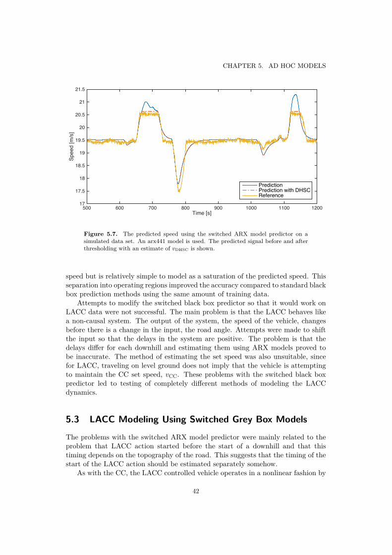
CHAPTER 5. AD HOC MODELS
Time [s]500 600 700 800 900 1000 1100 1200
Spee
d [m
/s]
17
17.5
18
18.5
19
19.5
20
20.5
21
21.5
PredictionPrediction with DHSCReference
Figure 5.7. The predicted speed using the switched ARX model predictor on asimulated data set. An arx441 model is used. The predicted signal before and afterthresholding with an estimate of vDHSC is shown.
speed but is relatively simple to model as a saturation of the predicted speed. Thisseparation into operating regions improved the accuracy compared to standard blackbox prediction methods using the same amount of training data.
Attempts to modify the switched black box predictor so that it would work onLACC data were not successful. The main problem is that the LACC behaves likea non-causal system. The output of the system, the speed of the vehicle, changesbefore there is a change in the input, the road angle. Attempts were made to shiftthe input so that the delays in the system are positive. The problem is that thedelays differ for each downhill and estimating them using ARX models proved tobe inaccurate. The method of estimating the set speed was also unsuitable, sincefor LACC, traveling on level ground does not imply that the vehicle is attemptingto maintain the CC set speed, vCC. These problems with the switched black boxpredictor led to testing of completely different methods of modeling the LACCdynamics.
5.3 LACC Modeling Using Switched Grey Box Models
The problems with the switched ARX model predictor were mainly related to theproblem that LACC action started before the start of a downhill and that thistiming depends on the topography of the road. This suggests that the timing of thestart of the LACC action should be estimated separately somehow.
As with the CC, the LACC controlled vehicle operates in a nonlinear fashion by
42

5.3. LACC MODELING USING SWITCHED GREY BOX MODELS
Time [s]800 900 1000 1100 1200 1300 1400 1500 1600 1700 1800
Spe
ed [m
/s]
23.4
23.6
23.8
24
24.2
24.4
24.6
24.8
25
25.2
25.4
PredictionReference
Figure 5.8. The predicted speed using the switched ARX model predictor on a reallife data set. An arx441 model is used. The same data set is used as presented inFigure 4.3.
switching between approximately linear behaviors. The problem is that road anglethresholding will not yield the transition points at which the system will be movingto another state.
Finding a method of estimating the transition points is challenging, since forevery downhill section, there will be only one data point for estimating the start ofa certain linear region. Driving over a single downhill can take a couple of minutes.The relation between the topography and the starting time is a complicated non-linear relation. Hence a lot of data is necessary to model this relation. This meansthat it is perhaps impossible to collect sufficient data to model the behavior of anHDV before it takes an exit or catches up to another vehicle. Two different methodsof estimating the delay are evaluated. One involves using an affine black box modelfor estimating the relation between some features of the topography and the otherone is based on the assumption that the LACC profiles are symmetric. Before welook at these methods, let us start with discussing the issue of estimating the setspeed.
5.3.1 Set Speed EstimationThe set speed estimation for LACC in the same manner as was done for CC isdifficult. For CC it was sufficient to know when the road can be considered flat and
43

CHAPTER 5. AD HOC MODELS
Road angle [rad]-0.04 -0.03 -0.02 -0.01 0 0.01 0.02 0.03 0.04
Acc
eler
atio
n [m
/s2]
-0.5
-0.4
-0.3
-0.2
-0.1
0
0.1
0.2
0.3
Figure 5.9. Plot showing how the dependence of the vehicle acceleration on theroad angle for a vehicle controlled by LACC. Different gears give rise the paralleldiagonal lines. One can also see that the transitions between the different gears arehighly irregular in terms of the road angle, making gear prediction very difficult.
then calculate the average of the speed when traveling over flat road sections.For LACC, the initial speed decrease below the set speed occurs frequently when
the ground is flat. If the speeds for flat road are averaged in the LACC case, theresult is a set speed estimate that is consistently too low.
To deal with this, it is assumed that set speed will be the most common speedthat the vehicle travels at. The set speed is then determined by creating a histogramof the speeds that the vehicle keeps. The mode of the histogram is then the setspeed estimate.
A histogram based method is more robust to this type of event. A histogram ismade over the top 10 % of the observed speeds. If there is a local maximum, thenthis is used as the vDHSC, otherwise, the greatest observed speed is used instead.
5.3.2 Prediction Using an Integrated Grey Box Model
For simulated data, the relation between the acceleration and the slope is linear atsome instances. Figure 5.9 shows the relation for the simulated data from Södertäljeto Norrköping. The downwards sloping straight line sections come from the uphillspeed dips and the downhill LACC profiles. The different lines correspond to dif-ferent gears at either maximum torque or with the clutch disengaged. Figure 5.9
44

5.3. LACC MODELING USING SWITCHED GREY BOX MODELS
justifies simplifying the equation of motion (3.11) to an affine equation in terms ofα as long as the vehicle acceleration is in one of the affine regions. The originalequation of motion is
mtota = keT − kav2 − kr cos(α) − kg sin(α). (5.6)
(5.6) can be reduced to affine form in α with a series of approximations. Using thesmall angle approximation sinα ≈ α and cosα ≈ 1. The air drag term kav
2 can beassumed to be constant since the time varying speed offset is fairly small comparedto constant set speed. Furthermore, torque and gear will be constant in a singleregion. The only non-constant term is then the gravitational force. The result isthat the equation of motion is simplified to
a = c1α+ c2, (5.7)
where a is the acceleration, α is the road angle and c1, c2 are unknown constants.An earlier concern from grey box modeling was that the noise from differentia-
tion made it difficult to estimate the parameters. Figure 5.10 shows what happensto the acceleration and road angle plot if a small amount of white Gaussian noiseis added to the speed prior to differentiation. The noise added to the speed has astandard deviation of 10−2 m/s. While it can be amended to some extent by filter-ing, it is better to avoid the differentiation step altogether to avoid noise problems.
It is therefore preferable to rewrite (5.7) in an integrated form in terms of speedinstead. Integrating 5.7 gives
v =∫ t
0(c1α+ c2)dτ, (5.8)
v = c1
∫ t
0αdτ + c2t. (5.9)
The coefficients c1 and c2 can still be easily determined using least squares, but nowin the time domain. Once the coefficients are known, the speed can be predicted byintegrating known road angles from road slope maps.
5.3.3 Estimating the Coefficients Online
The coefficients are estimated for each observed LACC profile. It is therefore nec-essary to detect LACC speed profiles. This is done in a similar manner to theestimation of the uphill and downhill speed deviations for CC.
It is assumed that the vehicle will always drive in the same gear and apply con-stant torque during an LACC profile. Commonly, the vehicle continuously coastswith the transmission either in neutral or in gear during the LACC speed adjust-ment. Unfortunately, this assumption is not always true and HDVs may changegear during an LACC profile.
45

CHAPTER 5. AD HOC MODELS
Road angle [rad]-0.04 -0.03 -0.02 -0.01 0 0.01 0.02 0.03 0.04
Acc
eler
atio
n [m
/s2]
-0.5
-0.4
-0.3
-0.2
-0.1
0
0.1
0.2
0.3
Figure 5.10. The relation between the road slope and the acceleration of an LACCcontrolled vehicle. This is the same data is used as in Figure 5.9 except that a smallamount of Gaussian noise was added to the speed prior to numeric differentiation.
The first step is to find the location of peaks and dips for observed speeds. Thechallenge is to only select peaks and dips that come from LACC speed profiles andnot from noise, gear shifts or uphill speed drops.
Figure 5.11 shows an idealized LACC speed profile. The negative peak of theLACC profile, at time tneg in the figure, occurs at the point when the downhillis sufficiently steep to cause the vehicle to accelerate. The positive peak, at timetpos, occurs when the downhill is no longer sufficiently steep to keep the vehicleaccelerating. Instead, the vehicle begins retarding due to drag and resistance.
The negative and positive peaks should occur at a specific angle when the netforce on the vehicle is zero. In (3.11), this occurs when the forces on the right handside sum to zero. The angle at which this occurs for a downhill will vary dependingon the speed of the vehicle and what torque/gear is being used.
Positive Peaks
In the case we are considering, when LACC is only used for downhills, large pos-itive peaks should only arise from LACC downhill speed profiles. There can bemany smaller peaks due to measurement noise and only sufficiently prominent peaksshould be considered. All positive peaks of sufficient prominence are therefore as-sumed to be LACC peaks.
46
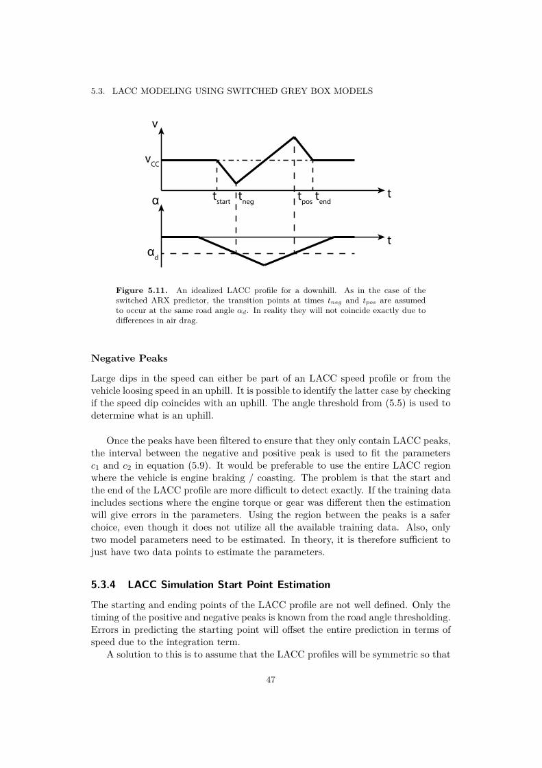
5.3. LACC MODELING USING SWITCHED GREY BOX MODELS
t
tα
v
αd
vCC
tneg tpoststart tend
Figure 5.11. An idealized LACC profile for a downhill. As in the case of theswitched ARX predictor, the transition points at times tneg and tpos are assumedto occur at the same road angle αd. In reality they will not coincide exactly due todifferences in air drag.
Negative Peaks
Large dips in the speed can either be part of an LACC speed profile or from thevehicle loosing speed in an uphill. It is possible to identify the latter case by checkingif the speed dip coincides with an uphill. The angle threshold from (5.5) is used todetermine what is an uphill.
Once the peaks have been filtered to ensure that they only contain LACC peaks,the interval between the negative and positive peak is used to fit the parametersc1 and c2 in equation (5.9). It would be preferable to use the entire LACC regionwhere the vehicle is engine braking / coasting. The problem is that the start andthe end of the LACC profile are more difficult to detect exactly. If the training dataincludes sections where the engine torque or gear was different then the estimationwill give errors in the parameters. Using the region between the peaks is a saferchoice, even though it does not utilize all the available training data. Also, onlytwo model parameters need to be estimated. In theory, it is therefore sufficient tojust have two data points to estimate the parameters.
5.3.4 LACC Simulation Start Point Estimation
The starting and ending points of the LACC profile are not well defined. Only thetiming of the positive and negative peaks is known from the road angle thresholding.Errors in predicting the starting point will offset the entire prediction in terms ofspeed due to the integration term.
A solution to this is to assume that the LACC profiles will be symmetric so that
47

CHAPTER 5. AD HOC MODELS
the positive and negative peaks have offsets from vCC of equal magnitude. Thisassumption is motivated by that most LACC controllers will try to maintain theaverage speed equal to vCC in order not to increase driving time. The problem withthis assumption is that it does not always hold, and some HDV manufacturers mayhave designed their LACC algorithm so that it is non-symmetric very often. If theassumption of symmetry is made, then the speed can be simulated outwards fromthe positive and negative peaks until it intersects vCC.
5.3.5 Uphill Model Estimation
The same model as for the LACC profiles, (5.9), can also be used to model thespeed drop due to uphills. The reason is that in a steep uphill, the torque shouldalso be constant since the vehicle will be applying maximum engine torque. Thesimplifications made to obtain the model (5.9) are therefore still valid. A problemis that the vehicle may shift to a lower gear during an uphill which occurs quitefrequently. The coefficients of the model from a different gear will result in poor fitin that case. The model coefficients are estimated on uphill speed drops detected inthe observed speed data. These areas are selected by choosing regions around thenegative peaks that correspond to positive road angles.
The method of determining the threshold angle for the uphills is similar to thatin Section 5.2.3. The difference is that for this model, it was chosen to detect thepeaks to avoid any error in the determination of the angle due to a speed threshold.Figure 5.12 shows a simplified illustration how the speed changes for LACC in anuphill. Determining the threshold angle for the uphills is done by detecting thenegative peaks in the observed speed that occur for positive road angles. The roadangles corresponding to all the measured peaks are averaged to obtain the thresholdangle.
The locations of the uphill dips are then predicted by thresholding the futureroad angles. The thresholding predicts the region from the start of the speed dipto the peak of the dip, i.e., between tstart and tpeak in Figure 5.12.
The speed of the target vehicle is then simulated for the predicted region using(5.9) and the estimated model coefficients. The region does not include the secondhalf of the speed dip between tpeak and tend. To include this region, the simulationusing the same coefficients is continued until it either intersects vCC or until theroad angle becomes negative.
5.3.6 DHSC Modeling
If the DHSC is not modeled as a separate state and is merely predicted as a satu-ration of the positive LACC peaks after they have been simulated, then the endingtime for the LACC profile will be incorrectly predicted as being much later thanit actually is. Such a misprediction will decrease the relative distance between thevehicles and risks collision.
48

5.3. LACC MODELING USING SWITCHED GREY BOX MODELS
t
tα
v
αu
vCC
tstart tpeak tend
Figure 5.12. An idealized LACC profile for an uphill. As previously, the transitionpoints at time tstart and tpeak are assumed to occur at the same road angle αu.
To ensure that the ending time is correct the DHSC is modeled as follows. If thesimulation of LACC profile reaches the estimated vDHSC value, then the simulationenters a DHSC state where the predicted output is vDHSC. The output is predictedas vDHSC until the road angle threshold for downhills is passed. At this pointthe LACC simulation using (5.9) resumes using vDHSC as the initial condition. Thesimulation terminates when it reaches vCC, the same way as for cases without DHSC.
The same method of estimating vDHSC as outlined in Section 5.2.2, can also beused for LACC. It involves using the maximal observed speed as the estimate forvDHSC. There is a problem with this approach. The radar that is used to measurethe speed, may give a spurious high reading that is much larger than vDHSC.
A histogram based method is more robust to this type of event. A histogram ismade over the top 10 % of the observed speeds. If there is a local maximum, thenthis is used as the vDHSC, otherwise, the greatest observed speed is used instead.
5.3.7 Alternative Start Time Prediction Using an Affine ModelAn attempt is made to predict the starting time of a LACC profile by modelingthe slope and the height as having an affine relation to the starting time. Thisis an alternative to assuming LACC profiles are symmetric as described in 5.3.4Using the terminology from Figure 5.11, let ∆t = tneg − tstart. The problem is thattstart does not occur at a well defined road angle as tneg and tpos do. Depending onexactly how the LACC algorithm is implemented in the target vehicle, the value of∆t will depend in a complicated way on the properties of the target truck and onthe topography of the road. The problem is that this relation is unknown and theproperties of the target truck are unknown.
The reason for using an affine model is that it is simple. The use of morecomplex models with more coefficients will require more training data. This would
49

CHAPTER 5. AD HOC MODELS
Height of downhill [m]0 10 20 30 40 50 60 70
"t [
s]
5
10
15
20
25
30
35
40
Figure 5.13. A plot of ∆t for downhill LACC speed profiles against the height ofeach downhill. The data is from the road between Södertälje and Norrköping.
go against one of the main objectives of this thesis which is reducing training time.The starting time is plotted against the average slope and the height of the
downhill to see if the use of an affine model is justified. Figure 5.13 shows ∆t heightof the downhill plotted against the height of the downhill. The height is definedas h = z(tneg) − z(tpos) if z(t) is the elevation of the road at time t. The relationappears to be affine, albeit with rather large variance. The correlation between ∆tand the height of the downhill for this data is 0.80. The height of the downhill isproportional to the potential energy lost in the downhill. The plot therefore showshow the LACC system selects ∆t for different potential energies lost in the downhill.Figure 5.14 shows the relation between ∆t and the average slope of the downhill forthe same data. The average slope is given by m = E[α(t)] for tneg ≤ t ≤ tpos. Theslope of the downhill is directly related to the force acting on the vehicle. Thereforethe plot illustrates the relation between the starting time and the average force dueto gravity on the vehicle. Measuring the correlation between the slope and ∆t forthis data set gives a value of -0.69. Based on these plots, it seems plausible that anaffine model may have some success predicting the starting time.
Equation (5.10) shows the suggested affine model that can be trained using ob-servations of average downhill slope m, downhill height h and starting time ∆t. Thecoefficients c1, c2 and c3 are unknown and should be estimated from the observa-
50
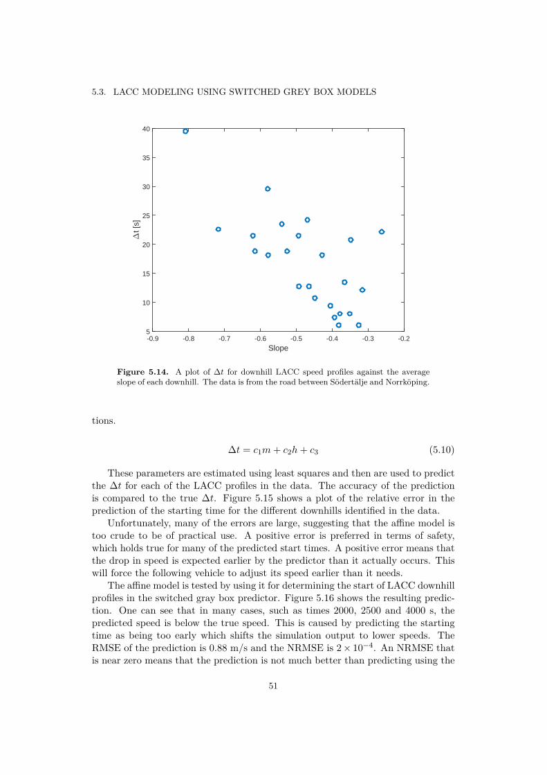
5.3. LACC MODELING USING SWITCHED GREY BOX MODELS
Slope-0.9 -0.8 -0.7 -0.6 -0.5 -0.4 -0.3 -0.2
"t [
s]
5
10
15
20
25
30
35
40
Figure 5.14. A plot of ∆t for downhill LACC speed profiles against the averageslope of each downhill. The data is from the road between Södertälje and Norrköping.
tions.
∆t = c1m+ c2h+ c3 (5.10)
These parameters are estimated using least squares and then are used to predictthe ∆t for each of the LACC profiles in the data. The accuracy of the predictionis compared to the true ∆t. Figure 5.15 shows a plot of the relative error in theprediction of the starting time for the different downhills identified in the data.
Unfortunately, many of the errors are large, suggesting that the affine model istoo crude to be of practical use. A positive error is preferred in terms of safety,which holds true for many of the predicted start times. A positive error means thatthe drop in speed is expected earlier by the predictor than it actually occurs. Thiswill force the following vehicle to adjust its speed earlier than it needs.
The affine model is tested by using it for determining the start of LACC downhillprofiles in the switched gray box predictor. Figure 5.16 shows the resulting predic-tion. One can see that in many cases, such as times 2000, 2500 and 4000 s, thepredicted speed is below the true speed. This is caused by predicting the startingtime as being too early which shifts the simulation output to lower speeds. TheRMSE of the prediction is 0.88 m/s and the NRMSE is 2 × 10⁻⁴. An NRMSE thatis near zero means that the prediction is not much better than predicting using the
51

CHAPTER 5. AD HOC MODELS
Downhills
Rel
ativ
e pr
edic
tion
erro
r [%
]
-60
-40
-20
0
20
40
60
80
100
120
Figure 5.15. The relative error in estimating the ∆t parameter for downhills onthe road from Södertälje to Norrköping. The downhills are ones that are sufficientlylarge to cause the vehicle to traverse them using an LACC speed profile. They arelisted on the horizontal axis in the order that they were encountered.
true average speed. In this comparison it seems that the affine model does not haveany advantage over assuming that the LACC curve is symmetric.
5.3.8 LACC Predictor TestingThe switched grey box predictor is tested on simulated data. The reference speed isobtained from a Scania simulation that accurately models the behavior of a vehiclewith an LACC controller. The simulation uses complex models of components suchas the gearbox, engine, axles etc. The road slope data for the simulation is theroad E4 between Södertälje and Norrköping. The training and testing datasets areshown in Figure 5.17. The training set was chosen so that it includes some drivingon level road and at least one uphill, one downhill and one use of DHSC.
The result of running the switched grey box predictor on this data set is shownin Figure 5.18. The RMSE for this prediction is 0.39 m/s, the NRMSE is 55 %. Aclose up version of Figure 5.18 is shown in Figure 5.19.
One can see a LACC profile starting at time 1700 that has a speed offset becausethe assumption that the profile is symmetric about vCC did not hold. Some of theother errors are a result of the vehicle shifting gears. This can be seen by lookingat the speed plot in Figure 5.18 and the gear plot in Figure 5.20 at 5000 s. Theprediction there has a large error when the gear is dropped down The very smallLACC profiles and uphill dips are often poorly predicted since the road angle forthem is very close to the threshold. Even quite small errors in estimating the
52

5.3. LACC MODELING USING SWITCHED GREY BOX MODELS
500 1000 1500 2000 2500 3000 3500 4000 4500 5000 5500
Spe
ed [m
/s]
15
20
25
Reference Prediction
Time [s]500 1000 1500 2000 2500 3000 3500 4000 4500 5000 5500
Roa
d A
ngle
[rad
]
-0.04
-0.02
0
0.02
0.04
Figure 5.16. Testing the affine model for LACC timing prediction by using it in theswitched gray box predictor.
0 1000 2000 3000 4000 5000 6000
Spe
ed [m
/s]
16
18
20
22
24
Training Testing
Time [s]0 1000 2000 3000 4000 5000 6000
Roa
d A
ngle
[rad
]
-0.06
-0.04
-0.02
0
0.02
Training Testing
Figure 5.17. The LACC speed data used for verifying the switched grey box predic-tor. The LACC speed is simulated using a Scania simulation environment. The roadslope data used in the simulation is from the road between Södertälje to Norrköping.
threshold angles will affect them. Due to the switching nature of the model, smallerdiscontinuities occur in some locations. If the MPC has problems with these, thenthey should be smoothed before use.
5.3.9 MPC Interfacing Test
The purpose of the predictor is to provide a prediction to an MPC controller whenthere is no V2V communications with the vehicle driving ahead. We will be using
53
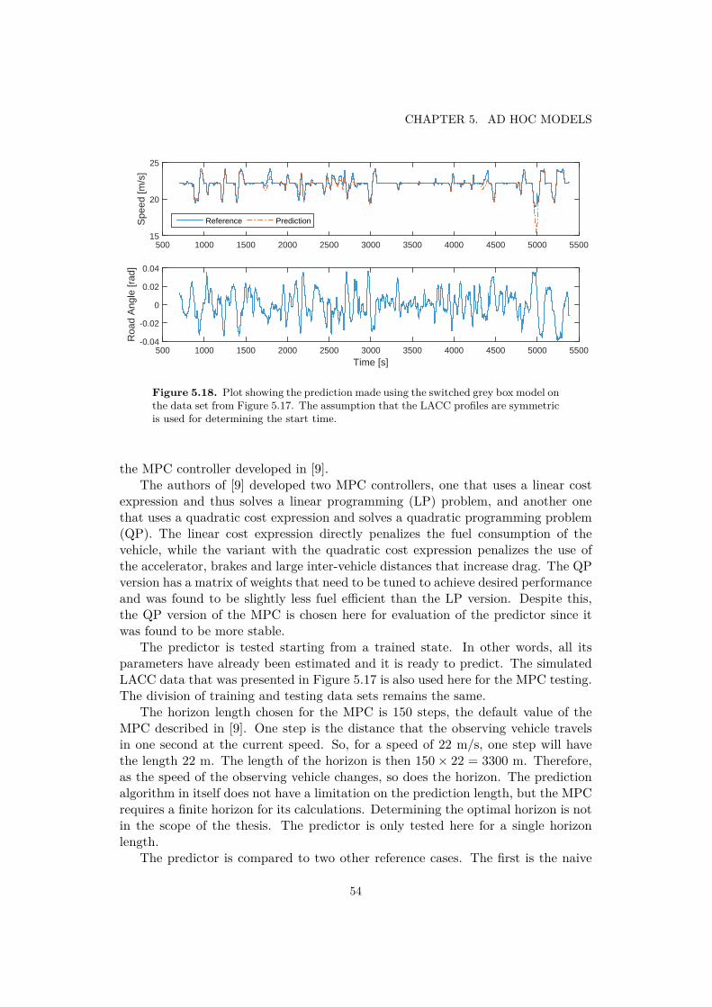
CHAPTER 5. AD HOC MODELS
500 1000 1500 2000 2500 3000 3500 4000 4500 5000 5500
Spe
ed [m
/s]
15
20
25
Reference Prediction
Time [s]500 1000 1500 2000 2500 3000 3500 4000 4500 5000 5500
Roa
d A
ngle
[rad
]
-0.04
-0.02
0
0.02
0.04
Figure 5.18. Plot showing the prediction made using the switched grey box model onthe data set from Figure 5.17. The assumption that the LACC profiles are symmetricis used for determining the start time.
the MPC controller developed in [9].The authors of [9] developed two MPC controllers, one that uses a linear cost
expression and thus solves a linear programming (LP) problem, and another onethat uses a quadratic cost expression and solves a quadratic programming problem(QP). The linear cost expression directly penalizes the fuel consumption of thevehicle, while the variant with the quadratic cost expression penalizes the use ofthe accelerator, brakes and large inter-vehicle distances that increase drag. The QPversion has a matrix of weights that need to be tuned to achieve desired performanceand was found to be slightly less fuel efficient than the LP version. Despite this,the QP version of the MPC is chosen here for evaluation of the predictor since itwas found to be more stable.
The predictor is tested starting from a trained state. In other words, all itsparameters have already been estimated and it is ready to predict. The simulatedLACC data that was presented in Figure 5.17 is also used here for the MPC testing.The division of training and testing data sets remains the same.
The horizon length chosen for the MPC is 150 steps, the default value of theMPC described in [9]. One step is the distance that the observing vehicle travelsin one second at the current speed. So, for a speed of 22 m/s, one step will havethe length 22 m. The length of the horizon is then 150 × 22 = 3300 m. Therefore,as the speed of the observing vehicle changes, so does the horizon. The predictionalgorithm in itself does not have a limitation on the prediction length, but the MPCrequires a finite horizon for its calculations. Determining the optimal horizon is notin the scope of the thesis. The predictor is only tested here for a single horizonlength.
The predictor is compared to two other reference cases. The first is the naive
54

5.3. LACC MODELING USING SWITCHED GREY BOX MODELS
Time [s]800 1000 1200 1400 1600 1800 2000 2200 2400 2600 2800
Spe
ed [m
/s]
19
20
21
22
23
24
ReferencePredictionv
DHSC estimate
Figure 5.19. Close up version of the speed plot in Figure 5.18 for times between 700and 2900 s. The dashed line shows the estimated value of the vDHSC that is used forDHSC modeling. The reference speed is generated by a controller that permits thespeed to exceed the set vDHSC for a short period of time. The predictor was designednot to model this behavior as it is not considered a general feature of an LACCalgorithm. The DHSC behavior observed here can be modeled more accurately byusing the maximum estimate from Section 5.3.6.
assumption that the target vehicle will maintain the current speed over the entireprediction horizon. This is a reasonable assumption if nothing is known aboutthe preceding vehicle behavior. The second case is the idealized case that thefuture speeds of the target vehicle are known perfectly. In reality, even with V2Vcommunication, knowing the future speed perfectly is not possible. These two casesshould give an indication of the relative performance of the case that uses thedeveloped predictor.
Figures 5.21 and 5.22 show the output of the MPC when the speed of the leadingvehicle is predicted using the switched grey box predictor. To see the equivalentoutput plots for the two reference cases, see Appendix B.
The performance of the predictor is evaluated by comparing its fuel consumptionto the two reference cases. The results of the fuel comparison are shown in Table 5.3.The limiting case that the predictor is able to perfectly predict the future speed ofthe target vehicle results in a 3.6 % lower fuel consumption. For the predictor, thisnumber is 2 %.
The fuel consumption figures will most likely depend on the desired followingdistance set in the MPC and if the vehicles have vastly different masses and max-imal torques. The desired following distance in this set of simulations is 24 m.
55
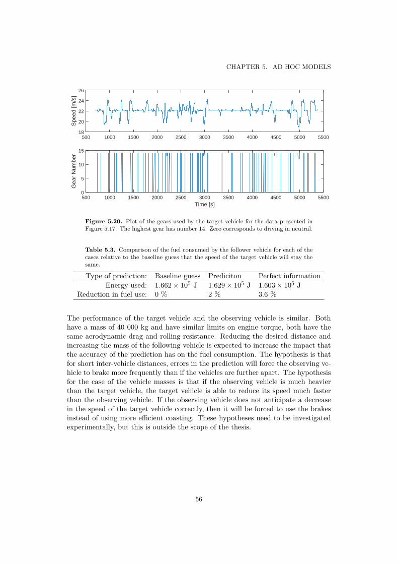
CHAPTER 5. AD HOC MODELS
500 1000 1500 2000 2500 3000 3500 4000 4500 5000 5500
Spe
ed [m
/s]
18
20
22
24
26
Time [s]500 1000 1500 2000 2500 3000 3500 4000 4500 5000 5500
Gea
r N
umbe
r
0
5
10
15
Figure 5.20. Plot of the gears used by the target vehicle for the data presented inFigure 5.17. The highest gear has number 14. Zero corresponds to driving in neutral.
Table 5.3. Comparison of the fuel consumed by the follower vehicle for each of thecases relative to the baseline guess that the speed of the target vehicle will stay thesame.
Type of prediction: Baseline guess Prediciton Perfect informationEnergy used: 1.662 × 10⁵ J 1.629 × 10⁵ J 1.603 × 10⁵ J
Reduction in fuel use: 0 % 2 % 3.6 %
The performance of the target vehicle and the observing vehicle is similar. Bothhave a mass of 40 000 kg and have similar limits on engine torque, both have thesame aerodynamic drag and rolling resistance. Reducing the desired distance andincreasing the mass of the following vehicle is expected to increase the impact thatthe accuracy of the prediction has on the fuel consumption. The hypothesis is thatfor short inter-vehicle distances, errors in the prediction will force the observing ve-hicle to brake more frequently than if the vehicles are further apart. The hypothesisfor the case of the vehicle masses is that if the observing vehicle is much heavierthan the target vehicle, the target vehicle is able to reduce its speed much fasterthan the observing vehicle. If the observing vehicle does not anticipate a decreasein the speed of the target vehicle correctly, then it will be forced to use the brakesinstead of using more efficient coasting. These hypotheses need to be investigatedexperimentally, but this is outside the scope of the thesis.
56

5.3. LACC MODELING USING SWITCHED GREY BOX MODELS
0 100 200 300 400 500 600 700
Spee
d [m
/s]
171819202122232425
Leader Reference MPC Output Leader Prediction
Time [s]0 100 200 300 400 500 600 700
Roa
d An
gle
[rad]
-0.04
-0.02
0
0.02
0.04
Figure 5.21. Plot of the speeds on the input and the output of the MPC when theleading vehicle speed is given by the switched grey box predictor. The input is theprediction of the leading/target vehicle, which is here compared to the true speed ofthe leading vehicle. The output of the MPC is the speed of the following/observingvehicle. Here, a simple saturation DHSC model is used. The bottom plot shows theroad angle for the leading vehicle.
57

CHAPTER 5. AD HOC MODELS
0 100 200 300 400 500 600 700
Rel
ativ
e D
ista
nce
[m]
0
20
40
60
0 100 200 300 400 500 600 700
Bra
king
For
ce [N
]
0
10 000
20 000
30 000
Time [s]0 100 200 300 400 500 600 700N
orm
aliz
ed E
ngin
e T
orqu
e
-0.5
0
0.5
1
Figure 5.22. The plots of the relative distance, braking force and engine torque forthe MPC when the leading vehicle speed is given by the switched grey box predictor.
58

Chapter 6
Discussion and Conclusion
The development of a speed predictor has resulted in an ad hoc model for CC con-trolled vehicles, and an ad hoc model for LACC controlled vehicles. Figure 6.1suggests a stucture for a complete preceding vehicle speed predictor. The compo-nents developed in this thesis are the CC predictor using the switched ARX methodand the LACC predictor using the switched grey box method. The parts that stillneed to be developed are the controller classifier and the human driver model.
6.1 Evaluation of Prediction Methods
All the methods considered here have the advantage that their prediction accuracydoes not drop off with time. As long as the vehicles being modeled do not changetheir properties while driving, there is no limit how far ahead in time one can predictthe speed. Of course, it is not relevant to attempt to predict the speed very faraway since surrounding traffic may induce different speed behavior, for example ifthe preceding vehicle catches up to another vehicle. When the predictor is usedin conjunction with an MPC for implementing cooperative cruise control then theprediction needs to only span the length of the MPC horizon.
6.1.1 Grey Box
Attempts at parameter estimation of the full vehicle dynamics model were unsuc-cessful. The large number of correlated parameters in the model made it difficult toestimate the parameters even when measurement noise was added. A further prob-lem, even if the vehicle dynamics could be estimated perfectly, was determining thecontroller. In the vehicle modeling experiments the engine and braking torque wereassumed to be known. Even if the structure of the controller is known, additionalparameters in the model cause even more difficulties with separating the contribu-tion of each parameter to the speed. Work by others also suggests that parameterestimation of the full vehicle model and controller system is a bad approach forpredicting the speed [7, 9].
59

CHAPTER 6. DISCUSSION AND CONCLUSION
Controller Classification
Statistical Model
Ad Hoc LACC Predictor
CC
LACC
Ad Hoc CC Predictor
HumanRoad slope data
Speed from radar
MPC
Interface
Figure 6.1. The suggested structure of the speed predictor for a preceding vehicle.The switched ARX predictor is the ad hoc CC predictor and the switched grey boxpredictor is the ad hoc LACC predictor. The figure is the same as Figure 1.2.
6.1.2 Black Box
This alternative method suggested was to directly predict the speed without creatinga physically motivated model. The main advantages of this is that the controllermodeling is no longer a separate problem, one that requires insight into how theleading vehicle is being controlled. The problem is that the switching behaviorof the speed controllers is highly nonlinear and requires quite advanced models toestimate it. These advanced models require large amounts of training data, whichmakes them impractical to use for predicting the speed of an unknown vehicle.
6.1.3 Switched ARX
To avoid the use of more complex neural network based black box models, thenonlinear switching behavior is modeled using a rule based algorithm to divide theprediction into linear regions. These linear regions can then be modeled using linearblack box models. This method has the advantage that it requires little trainingdata and yet can cope with the nonlinearity of the controller. The parametersthat are needed to be estimated were the coefficients of the two arx441 models, theuphill and downhill angle thresholds, the CC set speed vCC and the DHSC set speedvDHSC.
An inherent drawback of ad hoc solutions such as the rule based algorithmis that they are not very flexible. Ad hoc models tend to need a lot of tuningand tweaking before they behave as desired for many different types of input. Thepredictors designed in this thesis are based on how Scania has designed their controlalgorithms. An unexpected design of the control algorithm by some other HDVmanufacturer may cause the predictor to act in unexpected ways. In the case of theswitched ARX controller and CC modeling, the assumptions made for the rule basedalgorithm are still pretty general and should not differ a lot between manufacturers.
The switched ARX model was difficult to adapt to LACC data. The timingaspects of Scania’s LACC controller are difficult to model since the controller makesthe system behave non-causally and the timing of the start of the output dependsin a complex way on the topography of the upcoming road. Auto-regressive modelssuch as ARX can be cumbersome since they rely on previous outputs. This makesthem unsuitable for simulating backwards in time.
60

6.2. COMMENT ON THE DELIMITATIONS OF THE THESIS
6.1.4 Switched Grey Box
The switched grey box model has the advantage that it can be used to simulatebackwards in time and also has a high accuracy for well behaved cases. Only afew parameters need to be estimated for the switched grey box predictor. Theeight parameters that are needed are: the uphill and the downhill models withtwo parameters each, the CC set speed and the DHSC set speed, the road anglethreshold for uphills and the road angle threshold for downhills.
The main drawback of the switched grey box model is that it is less flexiblethan the switched ARX predictor. The predictor relies on some crude assumptions.Although the assumptions are physically motivated, it is still quite possible thatthey may not hold for HDVs made by other manufacturers. Since the behavior ofthe vehicle is assumed not to change during an uphill or a downhill, the predictordoes not handle gear changes very well. If the target vehicle shifts down by onlyone gear, the performance of the predictor is still acceptable. Thankfully, shiftingdown by more than one gear is not very frequent when driving on highways.
The main advantage of the switched grey box predictor is that it gives a quiteaccurate prediction using very little training data. It is sufficient to observe thetarget vehicle drive once over the type of feature one wants to predict. To fullytrain the predictor, one uphill, one downhill that reaches DHSC and some drivingat the CC set speed are sufficient. Since the model is approximately linear, a smallexcitation can be used to predict large ones. If only one uphill was observed, thenthe predictor should in theory be able to predict all uphills. Of course, this is notalways true due to noise and gear shifting.
The predictor can be easily expanded to also incorporate CC. The angle thresh-olds for the downhills are then determined, similarly to uphills, by observing roadangles for positive speed peaks. Estimating the model coefficients and predictingthe output are all done analogously to the uphill case.
6.2 Comment on the Delimitations of the ThesisIn this thesis, only a single leading vehicle has been considered. In real life, therecould be multiple vehicles driving ahead so that the behavior of the nearest leadingvehicle could be heavily influenced by the vehicles in front of it. Such scenariosare even more difficult to predict. There is a large amount of research in the areaof modeling car following behavior [14, 12, 13]. Many of these models may notbe suitable for modeling individuals as they are more directed at large scale trafficsimulations. These models are for human drivers and since they were designed forcars, they do not consider the effects of the road topography on the speed of thevehicle. If the leading vehicles are controlled by ACC then custom models need tobe used.
A common controller that was outside the scope of this thesis is the humandriver. There is unfortunately not much research on modeling truck driver behavior.Most driver models are car following models that do not consider one of the main
61

CHAPTER 6. DISCUSSION AND CONCLUSION
disturbances to regulating the speed on highways: the slope of the road. The idea ofcreating a statistical model of a human driver was considered but was not pursuedbecause of three main reasons. The first was that there were no suitable structuresfor modeling human truck drivers available, developing an own structure was beyondthe time frame of the thesis. The second concern is that a large variation betweendrivers is expected. A statistical model where some average driver is consideredmay not be very representative of how the driver ahead will behave. The thirdreason is that if one wants to model the specific driver that is driving ahead, thenit may require an unreasonably large amount of training data compared to a timeinvariant non-human regulator. The two latter concerns have not been tested andit is possible that they are unfunded.
6.3 ConclusionThis thesis has uncovered the complexity of the problem of predicting leading vehiclespeed. There are still many parts that should be investigated before a complete HDVspeed predictor is designed.
The work has shown that it is possible to achieve a large part of the possiblefuel reduction for an ideal case using practical methods. The presented switchedARX and grey box predictors illustrate how these nonlinear closed loop systemsencountered in HDV speed control can be divided into parts that are much easierto model. The switched grey box predictor is a promising base to build a moreuniversal speed predictor for both CC and LACC.
What remains before a complete HDV predictor can be designed is how humandriver behavior can be modeled, how gear shifting can be incorporated and howthe controller type should be identified. Human modeling will probably requirea completely different approach that is more statistically oriented and does notmodel a single individual but rather human drivers in general or in groups. Thestatistical approach is expected to result in much greater challenges in how it shouldbe interfaced to an MPC controller.
62

Chapter 7
Future Work
A considerable amount of work remains before a general speed predictor can bedesigned. This chapter summarizes the most important criteria for developing aspeed predictor and lists the areas where more work is required.
7.1 General Demands on the Speed PredictorThe following aspects are important to consider when developing a new speed pre-dictor:
Fuel saving potential - Increased overall accuracy of the predictor may notlead to greater fuel savings for the MPC. For instance, a prediction that isbetter at predicting sudden braking may be better than a prediction that ismore accurate overall but does not capture the sudden braking.
Prediction safety - It is safer to make predictions that make the observingvehicle take overly cautious speed choices. For example it is safer to expectthe braking in the downhill to be more sudden rather than more gradual. Ifthe predictions are too conservative then they may lead to a situation wherethe follower vehicle will loose the leader vehicle and will not be able to catchup, thus loosing any aerodynamic advantage.
Training time - A factor that limits the complexity of the models that can beused for speed prediction is the amount of training data that can be obtained.Complex models will require large amounts of data, the problem is that oneusually does not follow a single vehicle very long. The less time the modelneeds to to be trained, the longer it can be used for saving fuel.
Robustness - The model must be able to accommodate the variations in thecontrol algorithms of various manufacturers and be able to handle changes.
General vs. specific - One must be aware of the trade off between creating aspecific model and a general model. The specific model will have high accuracy
63

CHAPTER 7. FUTURE WORK
for a limited number of vehicles and requires that it is trained on the leadingvehicle. Making a model more general will reduce its accuracy since it willnot be able to predict all the peculiarities of the vehicle driving in front butis also applicable to a wider range of vehicles. This trade off goes thereforetogether with other considerations such as robustness and need of fine tuning.
7.2 Suggestions for Future Work
Human Driver Modeling
Human drivers are the main missing piece for a complete predictor. The frameworkfor modeling driver speed keeping behavior needs to be developed from scratch.There is not much earlier work in the area that is readily applicable to platooningof HDVs.
As mentioned earlier, human modeling will most probably require more generalstatistical models that model the average driver behavior for a certain topographicfeature. The problem is then finding a representation that allows generalizing datagathered from one downhill to be used for predicting speed on another.
Gear Prediction
Shifting can be identified by small speed drops during the gear change. It shouldbe possible to identify the gear shifts and then train separate parameters to eachgear that has been observed. The difficult part is then predicting which gear willbe used. It may be difficult to make a gear predictor that can be used for vehiclesof different brands yet needs only small amounts of training data. A typical HDVhas 14 gears. While typically only two or three are used on highways, potentiallymany models may be needed.
Controller Classification
The type of controller that the leading vehicle is using should be identified. Thesimplest approach is to run the predictors in parallel and see which one tends togive the best predictions for newly observed data. An alternative is to use machinelearning classification algorithms to determine which controller is being used.
MPC Interfacing
More statistical models may be difficult to interface to the MPC regulator of thefollower vehicle. For example methods that estimate the variance of the speed. Ifsuch a method is used, interpreting it in a suitable way for the MPC needs carefulconsideration.
64

7.2. SUGGESTIONS FOR FUTURE WORK
Background Investigations
One should investigate how the control algorithms differ between different manu-facturers, how the fuel saving potential changes depending on the proximity of thevehicles and depending on their relative masses and torques. Also, the length ofthe horizon used for the MPC should be analyzed in terms of fuel consumption andcomputational complexity.
65


Bibliography
[1] “European comission - vehicle categories.” Available at http://ec.europa.eu/clima/policies/transport/vehicles/docs/ec_hdv_ghg_strategy_en.pdf (2016-02-11).
[2] R. Muncrief and B. Sharpe, “Overview of the heavy-duty vehicle market andco2 emissions in the european union,” 2015.
[3] R. Muncrief and B. Sharpe, “Technology roadmap for the 21st century truckprogram. technical report 21ct-001,” 2000.
[4] E. Hellström, Look-ahead Control of Heavy Vehicles. PhD thesis, LinköpingUniversity, 2010.
[5] H. Felixson, “Vehicle ahead property estimation in heavy duty vehicles,” Mas-ter’s thesis, Linköpings Universitet, 2014.
[6] J. Slettengren, “Identification of target vehicle properties using acc-radar,”Master’s thesis, Uppsala Universitet, 2006.
[7] R. Hofwimmer and D. Lidander, “Vehicle motion and torque prediction for along haul truck,” Master’s thesis, 2014.
[8] A. Alam, Fuel-efficient heavy-duty vehicle platooning. PhD thesis, KTH RoyalInstitute of Technology, 2014.
[9] S. Freiwat and L. Öhlund, “Fuel-efficient platooning using road grade preview,”Master’s thesis, Uppsala Universitet, 2006.
[10] D. Arellano, T. Echaveguren, and S. Vargas-Tejeda, “A model of truck speedprofiles on short upward slopes,” in Proceedings of the Institution of CivilEngineers-Transport, vol. 168, pp. 475–483, Thomas Telford Ltd, 2014.
[11] C. Bester, “Truck speed profiles,” Transportation Research Record: Journal ofthe Transportation Research Board, no. 1701, pp. 111–115, 2000.
[12] P. G. Gipps, “A behavioural car-following model for computer simulation,”Transportation Research Part B: Methodological, vol. 15, no. 2, pp. 105–111,1981.
67

BIBLIOGRAPHY
[13] A. Levesque and J. Johrendt, “The state of the art of driver model develop-ment,” tech. rep., SAE Technical Paper, 2011.
[14] C. Cacciabue, Modelling Driver Behaviour in Automotive Environments: Crit-ical Issues in Driver Interactions with Intelligent Transport Systems. SpringerLondon, 2010.
[15] J. Junell and K. Tumer, “Robust predictive cruise control for commercial ve-hicles,” International Journal of General Systems, vol. 42, no. 7, pp. 776–792,2013.
[16] R. Rothery, R. Silver, R. Herman, and C. Torner, “Analysis of experiments onsingle-lane bus flow,” Operations Research, vol. 12, no. 6, pp. 913–933, 1964.
[17] A. Alam, A. Gattami, and K. H. Johansson, “An experimental study on thefuel reduction potential of heavy duty vehicle platooning,” in 13th Interna-tional IEEE Conference on Intelligent Transportation Systems (ITSC), 2010,pp. 306–311, IEEE, 2010.
[18] L. Bühler, “Fuel-efficient platooning of heavy duty vehicles through road to-pography preview information,” Master’s thesis, KTH Royal Institute of Tech-nology, 2013.
[19] L. Ljung and T. Glad, Modeling of dynamic systems. Prentice-Hall, 1994.
[20] L. Ljung, System identification - Theory for the User. Prentice-Hall, 1999.
68

Appendix A
CC Simulation in Simulink
69

APPENDIX A. CC SIMULATION IN SIMULINK
Figure
A.1.
Anoverview
figureoverthe
Simulink
structureused
tosim
ulatean
HDV
travelingover
acertain
topographicprofile
usingacruise
controllerwith
downhill
speedcontrol.
The
radarmeasurem
entsare
simulated
byadding
white
Gaussian
noisewith
avariance
correspondingto
theerrors
inGPSand
radar.
70
Appendix B
Plots for MPC Comparison Simulations
71

APPENDIX B. PLOTS FOR MPC COMPARISON SIMULATIONS
0 100 200 300 400 500 600 700
Spee
d [m
/s]
1819202122232425
Leader Reference MPC Output Leader Prediction
Time [s]0 100 200 300 400 500 600 700
Roa
d An
gle
[rad]
-0.04
-0.02
0
0.02
0.04
Figure B.1. Speed plot for the comparison case with the prediction assumption thatthe speed of the observed vehicle will stay the same. Note that the prediction curvehere only uses the displays the first step of the prediction at each time. The bottomplot is the corresponding road angle for the leader vehicle.
0 100 200 300 400 500 600 700
Rel
ativ
e D
ista
nce
[m]
0
20
40
60
0 100 200 300 400 500 600 700
Bra
king
For
ce [N
]
#104
0
0.5
1
1.5
2
Time [s]0 100 200 300 400 500 600 700N
orm
aliz
ed E
ngin
e T
orqu
e
-0.5
0
0.5
1
Figure B.2. The plots of the relative distance, braking force and engine torque forthe case with the assumption that the speed remains the same.
72

0 100 200 300 400 500 600 700
Spee
d [m
/s]
1819202122232425
Leader Reference MPC Output Leader Prediction
Time [s]0 100 200 300 400 500 600 700
Roa
d An
gle
[rad]
-0.04
-0.02
0
0.02
0.04
Figure B.3. Speed plot for the case of perfect information about the speed of theleading vehicle. The bottom plot shows the corresponding road angle for the leadervehicle.
0 100 200 300 400 500 600 700
Rel
ativ
e D
ista
nce
[m]
10
20
30
40
50
0 100 200 300 400 500 600 700
Bra
king
For
ce [N
]
0
5000
10000
15000
Time [s]0 100 200 300 400 500 600 700N
orm
aliz
ed E
ngin
e T
orqu
e
-1
-0.5
0
0.5
Figure B.4. The plots of the relative distance, braking force and engine torque forthe case of perfect information about the speed of the leading vehicle.
73

TRITA -EE 2016:122
ISSN 1653-5146
www.kth.se