Pre and Post-hoc Diagnosis and Interpretation of

Malignancy from Breast DCE-MRI

Gabriel Maicasa,1,∗, Andrew P. Bradleyb,1, Jacinto C. Nascimentoc,1,Ian Reida,2, Gustavo Carneiroa,1

aAustralian Institute for Machine Learning, The University of Adelaide, AustraliabScience and Engineering Faculty, Queensland University of Technology, Australia

cInstitute for Systems and Robotics, Instituto Superior Tecnico, Portugal

Abstract

We propose a new method for breast cancer screening from DCE-MRI basedon a post-hoc approach that is trained using weakly annotated data (i.e.,labels are available only at the image level without any lesion delineation).Our proposed post-hoc method automatically diagnosis the whole volumeand, for positive cases, it localizes the malignant lesions that led to suchdiagnosis. Conversely, traditional approaches follow a pre-hoc approach thatinitially localises suspicious areas that are subsequently classified to establishthe breast malignancy – this approach is trained using strongly annotateddata (i.e., it needs a delineation and classification of all lesions in an im-age). We also aim to establish the advantages and disadvantages of bothapproaches when applied to breast screening from DCE-MRI. Relying on ex-periments on a breast DCE-MRI dataset that contains scans of 117 patients,our results show that the post-hoc method is more accurate for diagnosingthe whole volume per patient, achieving an AUC of 0.91, while the pre-hocmethod achieves an AUC of 0.81. However, the performance for localisingthe malignant lesions remains challenging for the post-hoc method due tothe weakly labelled dataset employed during training.

∗Corresponding authorEmail address: gabriel.maicas@adelaide.edu.au (Gabriel Maicas )

1This work was partially supported by the Australian Research Council project(DP180103232). We would like to thank Nvidia for the donation of a TitanXp thatsupported this work.

2IR acknowledges the Australian Research Council: ARC Centre for Robotic Vision(CE140100016) and Laureate Fellowship (FL130100102)

Preprint submitted to Journal of Medical Image Analysis April 23, 2019

Keywords: magnetic resonance imaging, breast screening, meta-learning,few-shot learning, weakly supervised learning, strongly supervised learning,model interpretation, lesion detection, deep reinforcement learning.

1. Introduction

Breast cancer is amongst the most diagnosed cancers (AIHW, 2007; Siegelet al., 2017) affecting women worldwide (DeSantis et al., 2015; Torre et al.,2015). One of the most effective ways of increasing the survival rate for thisdisease is based on early detection (Saadatmand et al., 2015; Welch et al.,5

2016). Screening programs aim to provide such early detection by diagnos-ing at-risk, asymptomatic patients, allowing for an early intervention andtreatment. The most widely employed image modality for population-basedbreast screening is mammography. High risk patients are also recommendedto undergo screening with dynamically contrast enhanced magnetic resonance10

imaging (DCE-MRI) (Mainiero et al., 2017; Smith et al., 2017). DCE-MRIis known to increase the sensitivity, compared to mammography, especiallyin young patients that have denser breasts (Kriege et al., 2004).

However, the diagnosis and interpretation of DCE-MRI is a challengingand time consuming task that involves the interpretation of large amounts15

of data (Behrens et al., 2007) and is prone to high inter-observer variabil-ity (Grimm et al., 2015; Lehman et al., 2013). Computer-aided diagnosis(CAD) systems are designed to reduce the analysis time (Gubern-Meridaet al., 2016; Wood, 2005), increase sensitivity (Vreemann et al., 2018) andspecificity (Meinel et al., 2007), and serve as a second (automated) reader (Shi-20

mauchi et al., 2011). Designing such systems is challenging due to the vari-ability in location, appearance (Levman et al., 2009), size and shape (Songet al., 2016), and the low signal-to-noise ratio (Kousi et al., 2015) of lesions.In general, such CAD systems can be categorised as pre-hoc or post-hoc,depending on how the processing stages are organised, as explained below.25

Fully automated pre-hoc CAD methods for breast screening (Amit et al.,2017b; Dalmıs et al., 2018; Gubern-Merida et al., 2015) from DCE-MRIcompute the confidence score of malignancy of a breast using the follow-ing two-stage sequential approach: 1) detection of suspicious lesions, and 2)classification of the detected lesions. During detection (i.e., the first stage),30

the algorithm localises benign and malignant lesions, and possibly false pos-itive detections, in the image, which are then classified as malignant or non-malignant in the second stage. Four important challenges arise with this

2

(a) (b) (c)

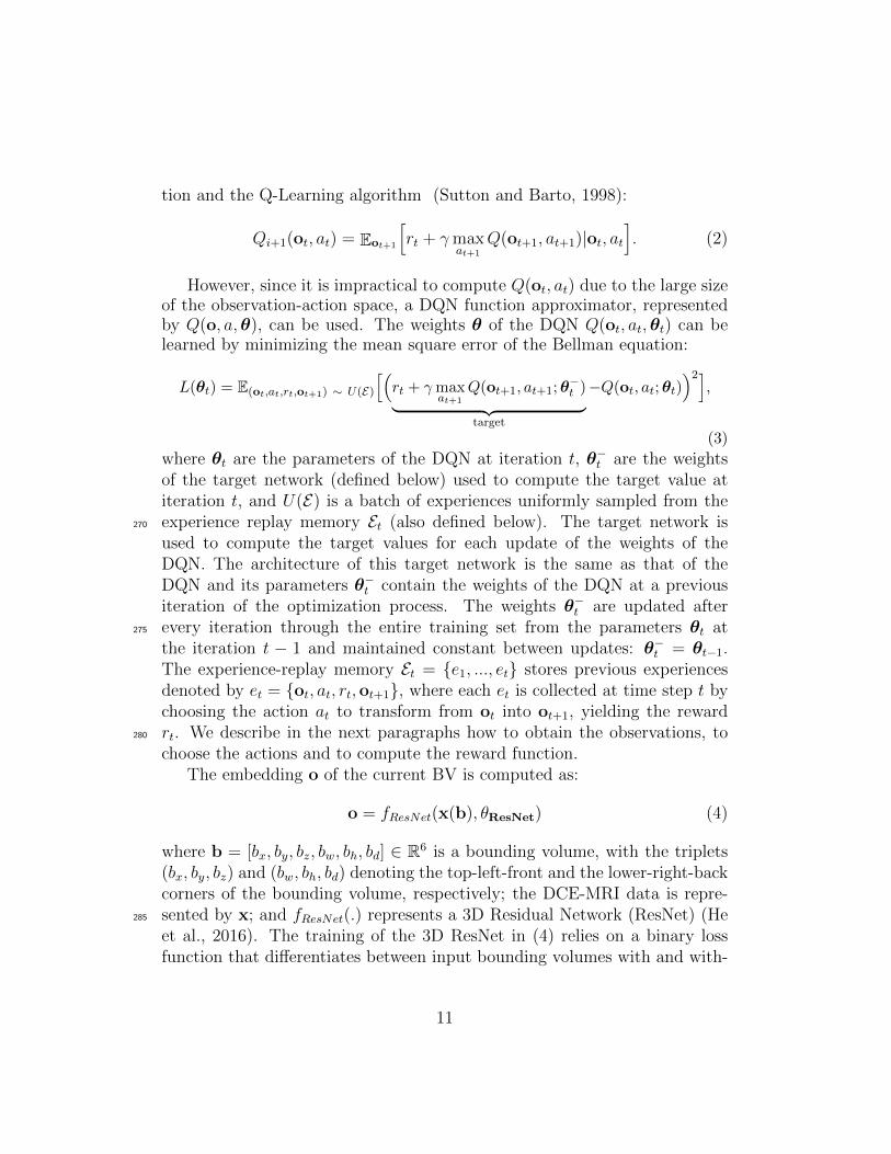
Figure 1: Example of a DCE-MRI breast image and annotation types. Image (1a) showsa slice of a breast DCE-MRI volume. Image (1b) shows the same slice with the strongannotations: lesion delineation classification as malignant. Image (1c) shows the weakannotation (i.e., whole image) of the same breast volume as malignant.

pre-hoc approach. Firstly, the modelling of the detector requires strong la-bels, i.e., precise voxel-wise annotation of lesions (see Fig. 1 for an example35

of different types of annotations). Strong annotation is expensive becauseit requires experts to label a relatively large number of training volumes; inaddition, given the difficulties involved in such manual labelling process, thisannotation may contain noise (this happens partly because experts are gen-erally not trained to provide such precise annotations in regular practice).40

Secondly, the classifier may be trained using incorrect manually annotatedlesion class labels. Such manual annotation is usually produced by biopsyanalysis, but if there are benign and malignant lesions jointly present in thesame breast, this analysis may not determine the correct association. Thirdly,apart from rare exceptions that need large annotated training sets (Ribli45

et al., 2018), pre-hoc diagnosis systems are generally trained in a two-stageprocess (Gubern-Merida et al., 2015; Mcclymont, 2015). This pipeline is notthe optimal way to maximise classification diagnosis performance becausethe final classification depends on the detection, but the detection optimal-ity does not warrant classification optimality. Finally, the fourth challenge is50

that the classification accuracy is limited by the detector performance, whereit is impossible for the classifier to recover from a missing lesion detectionbecause it can not be classified.

An alternative approach that is starting to gain traction (Esteva et al.,2017; Maicas et al., 2018; Wang et al., 2017a) reverses these stages. The first55

stage aims to classify the whole breast scan directly, followed by a second

3

stage that localizes regions in the scan that can explain the classification– for instance, if the first stage outputs a malignant diagnosis, then the

second stage aims to find malignant lesions in the scan. We term this apost-hoc approach. This approach is of special interest for the problem of60

breast screening from DCE-MRI because the whole-scan diagnosis can, forexample, analyse regions other than lesions that may contain relevant infor-mation for the diagnosis (Kostopoulos et al., 2017). The main advantage ofthese systems compared to pre-hoc systems is the possibility of using scan-level labels (referred to as weak labels in the rest of the paper). Such labels65

are already present in many Picture Archiving and Communication Systems(PACS) or can be automatically extracted from radiology reports (Wanget al., 2017a), eliminating almost completely the effort needed for the man-ual annotation described above for the pre-hoc approach. Also, the use ofscan-level labels overcomes the limitations in annotations required by pre-70

hoc approaches. Firstly, there is no need for lesion delineation avoiding suchcostly process. Secondly, the incorrect labelling of lesions explained above isreduced as the most likely lesion to be malignant is biopsied and thereforethe label is more likely to be correct –there is no need to associate labelswith lesions. The main challenge of post-hoc systems resides in highlighting75

the scan regions that can justify a particular classification (e.g., in the caseof a malignant classification, it is expected that the regions represent themalignant areas of the scan), given that such manual annotation is not avail-able. This challenge is important for the deployment of post-hoc systems inclinical practice (Caruana et al., 2015).80

In this paper, we propose a new post-hoc method and a systematic com-parison between pre-hoc and post-hoc approaches for breast screening fromDCE-MRI. We aim to answer the following research questions: 1) whichapproach should be chosen if the goal is to optimally classify a whole scanin terms of malignant or non-malignant findings, and 2) how accurate is85

the localisation of malignant lesions produced by post-hoc approaches whencompared with the localisation of malignant lesions produced by pre-hocmethods. The pre-hoc system considered in this paper is based on our re-cent detection model (Maicas et al., 2017b) that achieves state-of-the-art(SOTA) lesion localisation, while reducing the inference time needed by tra-90

ditional exhaustive search methods. For the post-hoc system, we rely onour recently proposed approach based on meta-learning (Maicas et al., 2018)that holds the SOTA performance for the problem of breast screening fromDCE-MRI. Decision interpretation is based on our recent 1-class saliency

4

detector (Maicas et al., 2019), especially designed for the weakly supervised95

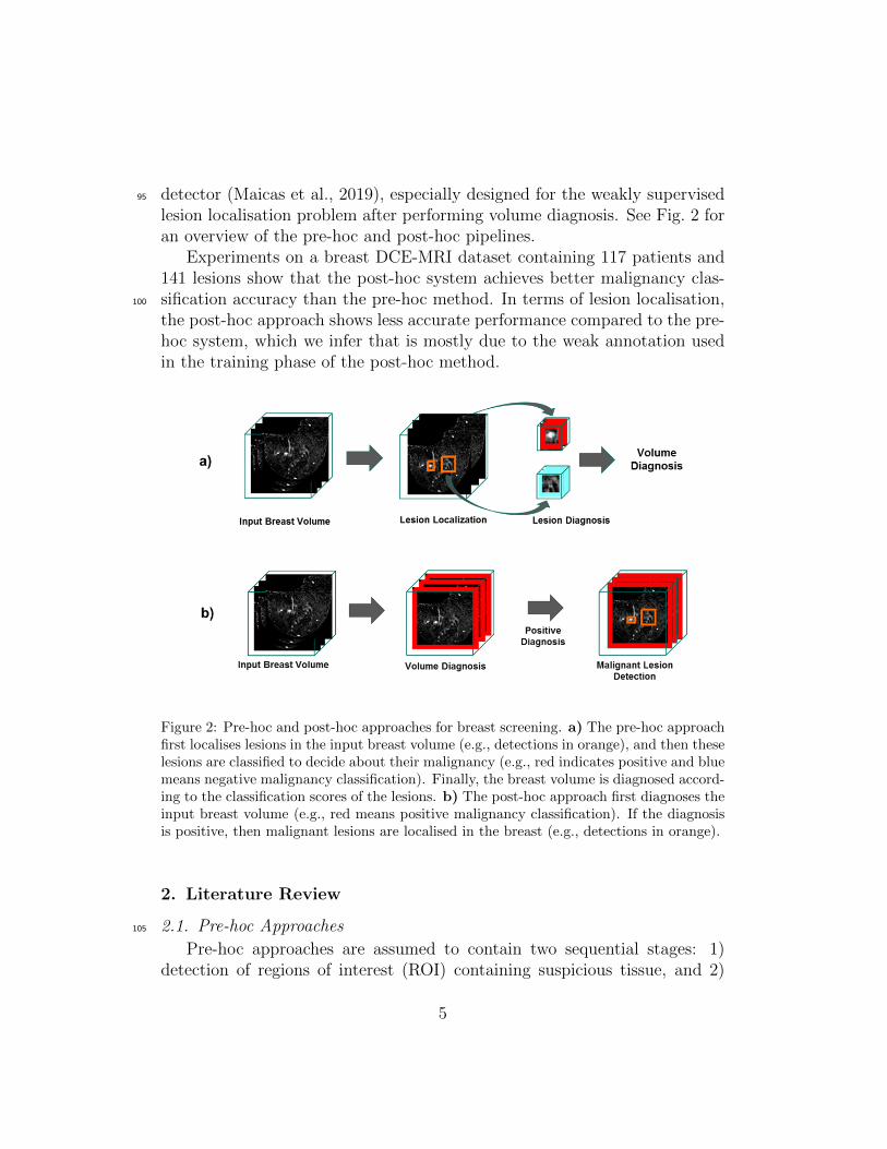
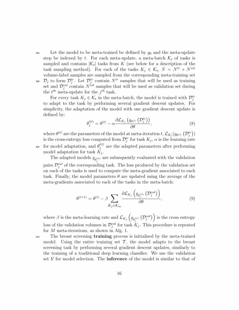
lesion localisation problem after performing volume diagnosis. See Fig. 2 foran overview of the pre-hoc and post-hoc pipelines.

Experiments on a breast DCE-MRI dataset containing 117 patients and141 lesions show that the post-hoc system achieves better malignancy clas-sification accuracy than the pre-hoc method. In terms of lesion localisation,100

the post-hoc approach shows less accurate performance compared to the pre-hoc system, which we infer that is mostly due to the weak annotation usedin the training phase of the post-hoc method.

Figure 2: Pre-hoc and post-hoc approaches for breast screening. a) The pre-hoc approachfirst localises lesions in the input breast volume (e.g., detections in orange), and then theselesions are classified to decide about their malignancy (e.g., red indicates positive and bluemeans negative malignancy classification). Finally, the breast volume is diagnosed accord-ing to the classification scores of the lesions. b) The post-hoc approach first diagnoses theinput breast volume (e.g., red means positive malignancy classification). If the diagnosisis positive, then malignant lesions are localised in the breast (e.g., detections in orange).

2. Literature Review

2.1. Pre-hoc Approaches105

Pre-hoc approaches are assumed to contain two sequential stages: 1)detection of regions of interest (ROI) containing suspicious tissue, and 2)

5

classification of ROIs into malignant or not malignant (benign and/or falsepositive) tissue.

Traditional pre-hoc approaches for breast screening from breast DCE-110

MRI were based on manual (Agner et al., 2014; Gallego-Ortiz and Martel,2015; Mus et al., 2017; Soares et al., 2013) or semi-automated (Chen et al.,2006; Dalmıs et al., 2016; Meinel et al., 2007; Milenkovic et al., 2017; Platelet al., 2014) ROI detection. In addition, the classification in these traditionalapproaches was based on support vector machine (SVM), random forest, or115

artificial neural network models, using hand-designed features (e.g., dynamic,morphological, textural or multifractal) (Dalmıs et al., 2016; Meinel et al.,2007; Milenkovic et al., 2017; Platel et al., 2014).

Aiming at reducing user intervention to reduce the number of ROIs (Liuet al., 2017), pre-hoc systems evolved to be fully automated. Such automated120

pre-hoc approaches generally employed an exhaustive search method or clus-tering to detect ROIs in the scan using hand-designed features (Gubern-Merida et al., 2015; Mcclymont, 2015; Renz et al., 2012; Wang et al., 2014).The classification of ROIs into false positive, benign or malignant findingsis then performed with a new set of hand-designed features extracted from125

the ROIs (Gubern-Merida et al., 2015; Mcclymont, 2015; Renz et al., 2012;Wang et al., 2014). These fully automated methods generally suffer fromtwo issues: 1) the sub-optimality of hand-designed features needed at bothROI localization and ROI classification, and 2) the high computational costof the exhaustive search to detect ROIs.130

Both limitations have been addressed after the introduction of deep learn-ing methodologies (Krizhevsky et al., 2012) in the field of medical imageanalysis. Initially, feature sub-optimality was addressed either for ROI de-tection (Maicas et al., 2017a,b) or classification (Amit et al., 2017a,b; Rastiet al., 2017), but it was recently solved for both detection and classifica-135

tion (Dalmıs et al., 2018). Dalmıs et al. (2018) also reduced the inferencetime of the exhaustive search by directly computing a segmentation mapfrom the scan using a U-net (Ronneberger et al., 2015).

Although each step of the pipeline has been individually optimized, thereis no guarantee that the full pipeline is optimal in terms of classification140

accuracy. This was addressed with the formation of large datasets that hasenabled the use of SOTA one-stage detection and classification computer vi-sion techniques, such as Faster R-CNN (Ren et al., 2015) or Mask RCNN (Heet al., 2017). The main advantage of these methods lies in the optimality ofthe end-to-end training, effectively merging the detection and classification145

6

tasks (Dalmıs et al., 2018). For example, Ribli et al. (2018) applied FasterR-CNN to detect tumours from mammograms and they showed that this ap-proach is quite efficient in terms of inference time. However, Faster R-CNNgeneralises poorly, which means that the training set must contain a largeannotated set of ROIs and, at the same time, be rich enough to comprise150

all possible lesion variations. Besides the need for large datasets, which aredifficult to acquire for DCE-MRI breast screening, these systems suffer fromthe need for strong annotations (i.e., the accurate delineation of the lesions).Li et al. (2018) partially addressed this issue by developing a semi-supervisedsystem, alleviating the need of lesion annotations. However, a large number155

of annotated images (880) is still required to train the system.

2.2. Post-hoc Approaches

Post-hoc systems aim to overcome the need for strong annotations bytraining models with only scan-level labels (i.e., weak labels). This is es-pecially useful for the problem of breast screening, where the analysis of160

adjacent regions to lesions may be important (Kostopoulos et al., 2017). Inaddition, the classification accuracy of post-hoc systems are not constrainedby the lesion detection, which is the case in pre-hoc systems.

Several post-hoc systems have been proposed (Wang et al., 2017a; Zhuet al., 2017). For instance, Wang et al. (2017a) use a deep learning model to165

produce classification scores from whole scans and Zhu et al. (2017) propose adeep multiple instance learning. However, these approaches still require largedatasets to achieve good performance. This issue was addressed by Maicaset al. (2018), who proposed a new meta-learning methodology to learn froma small number of annotated training images. Their work established a new170

SOTA classification accuracy for breast screening from DCE-MRI.The main challenge for post-hoc models arises from the fact that they

do not use manually annotated ROIs for training, which makes the ROI lo-calisation (and delineation) a hard task. Such ROI localisation is importantfor explaining the classification made by the CAD system in clinical settings175

(e.g., for a scan classified as malignant, doctors are likely to know where thelesions are located). Solving this lesion localisation problem is a researchproblem that is being actively investigated in the field (Dubost et al., 2017;Feng et al., 2017; Maicas et al., 2019; Wang et al., 2017b; Yang et al., 2017).The approach proposed by Maicas et al. (2019) achieves SOTA detection per-180

formance by properly defining saliency for the problem of weakly supervised

7

lesion localisation, which assures that salient regions represent malignantlesions in the image.

However, the literature does not provide any studies comparing pre andpost-hoc diagnosis approaches. The main reason for this absence of com-185

parison among the methods described in this literature review is that suchanalysis is not straightforward due to (Maicas et al., 2017b): 1) the lack ofpublicly available datasets that can be used to compare new approaches to thecurrent state-of-the-art, 2) the criteria to decide if an ROI is a true positivedetection, and 3) the criteria to decide if lesions labelled as the challenging190

BIRADS=3 should be included into the benign category (Gubern-Meridaet al., 2015). In addition, not all assessments of pre-hoc fully automatedmethodologies consider false positives in the diagnostic stage as they onlydifferentiate between benign and malignant (Mcclymont, 2015). We pro-pose to compare both types of automated approaches for the problem of195

breast screening from breast DCE-MRI. With the use of a common datasetand well-defined criteria to satisfy the issues described above, we investigatewhich approach performs better for breast diagnosis and lesion localisation.

3. Methods

This section provides a formal description of the dataset in Sec. 3.1, the200

pre-hoc method in Sec. 3.2, and the post-hoc approach in Sec. 3.3.

3.1. Dataset

Let D =(

bi,xi, ti, s(j)i

Mj=1, l

(j)i

Mj=1,yi

)i

i∈1,...,|D|,bi∈left,right

denote the 3D DCE-

MRI dataset, where bi ∈ left, right specifies the left or right breast of the ith

patient; xi, ti : Ω → R represent the first 3D DCE-MRI subtraction volume205

and the T1-weighted MRI volume used for preprocessing, respectively, withΩ ∈ R3 representing the volume lattice of size w × h× d; s

(j)i : Ω→ 0, 1 is

the voxelwise annotation of the jth lesion present in the breast bi (s(j)i (ω) = 1

indicates the presence of lesion in voxel ω ∈ Ω, and s(j)i (ω) = 0 denotes the

absence of lesion); l(j)i Mj=1 ∈ 0, 1 indicates the classification of lesion j as210

benign or malignant, respectively; and yi is a scan-level label with the follow-ing values: yi = 0 if there is no lesion in breast bi, yi = 1 if all the lesion(s)in breast bi are benign or yi = 2 if there is at least one malignant lesion.The dataset is patient-wise split into train T , validation V and test U sets,such that images of each patient only belong to one of the sets. Note that the215

8

voxelwise lesion annotations s(j)i Mj=1 and l(j)i Mj=1 are not employed duringthe training of the post-hoc system – they are only used to train and testthe pre-hoc system and in the quantification of the results for both systems.Finally, the motivation behind the use of the first subtraction image x liesin the reduction of cost and time for image acquisition and analysis (Gilbert220

and Selamoglu, 2018; Mango et al., 2015).

3.2. Pre-hoc Method

Our proposed pre-hoc approach is based on the following steps:

1. Lesion detection (Sec. 3.2.1): an attention mechanism based on deepreinforcement learning (DRL) (Mnih et al., 2015) searches for lesions225

using a method that analyses large portions of the breast volume anditeratively focuses the search on the appropriate regions of the inputvolume.

2. Lesion diagnosis (Sec. 3.2.2): a state-of-the-art deep learning classi-fier (Huang et al., 2017) analyses the lesions detected in the previous230

step in order to classify them as malignant or non-malignant (note thatnon-malignant regions are represented by benign lesions or normal tis-sue, i.e. false positive detections). The confidence score of malignancyfor the breast volume is defined as the maximum probability of malig-nancy among the detected lesions.235

3.2.1. Lesion Detection

We propose an attention model that is capable of reducing the infer-ence time of previous methods for lesion detection (Gubern-Merida et al.,2015; McClymont et al., 2014) in pre-hoc systems. This attention mecha-nism searches for lesions by progressively transforming relatively large initial240

bounding volumes (BV) (i.e. sub-regions of the MRI volume) into smallerregions containing a more focused view of potential lesions (Maicas et al.,2017b). The transformation process is guided by a policy π that indicateshow to optimally change the current BV to detect a lesion. The policy isrepresented by a deep neural network, called deep Q-net (DQN), that re-245

ceives as input an embedding vector o ∈ RO of the current BV and outputsa measurement (i.e., the Q-value (Q)), representing the optimality associatedwith each of the possible transformations to find a lesion. See Figure 3 for ablock diagram of this process. The aim of the learning phase is to model suchpolicy, i.e., find the optimal parameters of the DQN. The inference exploits250

the policy to detect the lesions present in a breast DCE-MRI volume.

9

Figure 3: Overview of the proposed lesion detection method. The bounding volume of thecurrent observation is extracted from the input breast volume and fed to the 3D ResNetto obtain the embedding of the observation. The embedding is then forwarded throughthe Q-net to obtain the Q-values for each of the actions.

The training process of the DQN follows that of a traditional MarkovDecision Process (MDP), which models a sequence of decisions to accomplisha goal from an initial state. At every time step, the current BV, representedby the observations o, will be transformed by an action a, yielding a reward255

r – this reward indicates the effectiveness of the chosen transformation fordetecting a lesion. The goal is to learn what actions should be applied totransform the current observation to another one with larger Dice coefficientmeasured with respect to the target lesion. In an MDP set-up, this translatesinto choosing the action that maximizes the expected sum of discounted260

future rewards (Mnih et al., 2015): Rt =∑T

t′=t γt′−trt′ , where γ ∈ (0, 1) is a

discount factor.Let Q?(o, a) be the optimal Action-Value Function representing the ex-

pected sum of discounted future rewards by choosing action a to transformthe observation o. The optimal Action-Value function follows the policy π,as in:

Q?(o, a) = maxπ

E[Rt|ot = o, at = a, π]. (1)

Intuitively, Q?(.) represents the quality of performing the action a given thecurrent observation o to achieve the final goal. Therefore, the goal of thetraining process is to learn Q?(.), which maximizes the commulative sum of265

expected discounted rewards.The optimalQ?(o, a) can be computed iteratively using the Bellman equa-

10

tion and the Q-Learning algorithm (Sutton and Barto, 1998):

Qi+1(ot, at) = Eot+1

[rt + γmax

at+1

Q(ot+1, at+1)|ot, at]. (2)

However, since it is impractical to compute Q(ot, at) due to the large sizeof the observation-action space, a DQN function approximator, representedby Q(o, a,θ), can be used. The weights θ of the DQN Q(ot, at,θt) can belearned by minimizing the mean square error of the Bellman equation:

L(θt) = E(ot,at,rt,ot+1) ∼ U(E)

[(rt + γmax

at+1

Q(ot+1, at+1;θ−t )︸ ︷︷ ︸

target

−Q(ot, at;θt))2]

,

(3)

where θt are the parameters of the DQN at iteration t, θ−t are the weightsof the target network (defined below) used to compute the target value atiteration t, and U(E) is a batch of experiences uniformly sampled from theexperience replay memory Et (also defined below). The target network is270

used to compute the target values for each update of the weights of theDQN. The architecture of this target network is the same as that of theDQN and its parameters θ−t contain the weights of the DQN at a previousiteration of the optimization process. The weights θ−t are updated afterevery iteration through the entire training set from the parameters θt at275

the iteration t − 1 and maintained constant between updates: θ−t = θt−1.The experience-replay memory Et = e1, ..., et stores previous experiencesdenoted by et = ot, at, rt,ot+1, where each et is collected at time step t bychoosing the action at to transform from ot into ot+1, yielding the rewardrt. We describe in the next paragraphs how to obtain the observations, to280

choose the actions and to compute the reward function.The embedding o of the current BV is computed as:

o = fResNet(x(b), θResNet) (4)

where b = [bx, by, bz, bw, bh, bd] ∈ R6 is a bounding volume, with the triplets(bx, by, bz) and (bw, bh, bd) denoting the top-left-front and the lower-right-backcorners of the bounding volume, respectively; the DCE-MRI data is repre-sented by x; and fResNet(.) represents a 3D Residual Network (ResNet) (He285

et al., 2016). The training of the 3D ResNet in (4) relies on a binary lossfunction that differentiates between input bounding volumes with and with-

11

out lesions. The dataset to train this 3D ResNet is built by sampling randomBVs that are labelled as positive if the Dice Coefficient with a ground truthlesion is larger than 0.6, and negative otherwise. We empirically found that290

such a relatively large threshold of 0.6 helped the model to focus more tightlyon the lesions during the training process. Note that the training of the 3DResNet with a potentially infinite number of BVs from different scales, sizesand locations allows us to obtain a rich collection of BVs without the needfor a large training set.295

The setA = l+x , l−x , l+y , l−y , l+z , l−z , s+, s−, w represents the actions to mod-ify the current BV, where l, s, w represent the translation, scale and trig-ger (to terminate the search for lesions) actions, respectively; the subscriptsx, y, z denote the horizontal, vertical and depth translation, and the super-scripts +,− represent the positive/negative translation or up/down scal-300

ing.The reward function depends on the improvement in the lesion localisa-

tion process after selecting a specific action. For action a ∈ A \ w, wemeasure the improvement in terms of the variation of the Dice coefficientafter applying action a to transform the observation ot to ot+1:

r(ot, a,ot+1) = sign(d(ot+1, s)− d(ot, s)), (5)

where d(.) is the Dice coefficient between the bounding volume o and theground truth s. The intuition behind (5) is that the reward is positive if theDice coefficient from observation ot to observation ot+1 increases, and thereward is negative otherwise. The quantization in (5) avoids a deterioration of305

the training convergence due to small changes in d(.) (Caicedo and Lazebnik,2015).

The reward for the trigger action, a = w, is defined as:

r(ot, a,ot+1) =

+η if d(ot+1, s) ≥ τw

−η otherwise(6)

where η > 1 encourages the trigger action to finalize the search for lesionsif the Dice coefficient with the ground truth s is larger than a pre-definedthreshold τw.310

Actions during the training process are selected according to a modified ε-greedy strategy to balance exploration and exploitation (Maicas et al., 2017b):with probability ε, a random action will be explored, and with probability

12

1− ε, the action will be chosen from the current policy. During exploration,with probability κ, a random action is selected, and with probability 1−κ, a315

random action from the actions that will produce a positive reward is selected.During exploitation, the action is selected according to the current policy:at = arg maxat Q(ot, at;θt). The training process starts with ε = 1, whichdecreases linearly, transitioning from pure exploration to mostly exploitationfollowing the current policy as the model learns to detect lesions.320

During inference, we exploit the learned policy to detect lesions. In prac-tice, we propose several initial bounding volumes covering different relativelylarge portions of the DCE-MRI volume. Each initialization is processed inde-pendently and is iteratively transformed according to the action a?t indicatedby the optimal action-value function:

a?t = arg maxat

Q(ot, at;θ?). (7)

where θ? represents the parameter vector of the trained DQN model learnedwith (3).

We define the set of detected lesions as Dpre = Dprei |Dpre|i=1 , where Dprei

represents the ith bounding volume, when the trigger action is selected to stopthe inference process. If the trigger action is not selected after 20 iterations,325

the search for a lesion is stopped yielding no detection.

3.2.2. Lesion diagnosis

The detected lesions in Dpre, formed during the lesion localization stage,are classified in terms of their malignancy. This binary classification is per-formed with a 3D DenseNet (Huang et al., 2017), trained using the detections330

from the training set to differentiate normal tissue and benign lesions (i.e.,negative diagnoses) from malignant lesions (positive diagnosis). During in-ference, each detection Dprei is fed through the 3D DenseNet to obtain itsprobability of malignancy. Finally, the confidence score of malignancy ofa breast is defined as the maximum of the malignancy probabilities com-335

puted from all the detected regions in such breast. The confidence score ofmalignancy for the breast volume with no detections is set to zero.

3.3. Post-hoc Method

Our proposed post-hoc approach is characterised by the following steps:

1. Diagnosis (Sec. 3.3.1): the classifier outputs the probability that a340

breast DCE-MRI volume contains a malignant lesion. Given the small

13

training dataset, the model is first meta-trained with a teacher-studentcurriculum learning strategy to learn to solve several tasks. Then, theclassifier is fine-tuned to solve the breast screening diagnosis task.

2. Lesion Localization (Sec. 3.3.2): the detector is weakly-trained to345

localise malignant lesions on breast DCE-MRI volumes that have beenpositively classified in the diagnosis stage above. This lesion localisa-tion process can be used to interpret the decision from the diagnosisstage.

3.3.1. Breast Volume Diagnosis350

Meta-training aims to learn a model that can solve new given tasks (clas-sification problems) as opposed to traditional classifiers that solve a specificclassification problem. Traditionally, models for solving new tasks have beenachieved by fine-tuning pre-trained models (Tajbakhsh et al., 2016). How-ever, these pre-trained models are rarely available for 3D volumes and large355

datasets are still required. These limitations can be overcome by including ameta-training phase before training, where the model is presented with sev-eral classification tasks that need to be solved, where each task has a smalltraining set. Eventually, the model learns to solve new tasks that containsmall training sets.360

As noted in our previous work (Maicas et al., 2018), the order in which topresent classification tasks during meta-training influences the ability of themodel to solve new tasks. Therefore, we propose to use the teacher-studentcurriculum learning strategy (Matiisen et al., 2017) that has been shown tooutperform other strategies (Maicas et al., 2018).365

We propose to meta-train the model to solve several related classificationtasks, each containing a relatively small number of training images instead oftraining a classifier to distinguish volumes with any malignant findings fromothers containing no malignant lesions. Firstly, during the meta-trainingphase, our model learns to solve different tasks that are formed from our370

breast DCE-MRI datasets. The tasks to be presented to the model are se-lected via the teacher-student curriculum learning strategy and contain asmall training set. Secondly, the training phase is similar to that of anytraditional classifier and solves the breast screening task using the samplesavailable from the training set. The difference in our approach lies in the375

employment of the meta-trained model as the initialization for the train-ing process. As a result, when the meta-trained model is fine-tuned on thebreast screening task with the small training set, it is able to efficiently

14

and effectively classify previously unseen volumes containing malignant find-ings (Maicas et al., 2018). Finally, the inference phase (or breast diagnosis)380

consists of feeding the input volumes to the classifier to estimate the proba-bility that they contain a malignant finding. See Figure 4 for an overview ofthe volume diagnosis process.

Figure 4: Volume diagnosis process. Firstly, the model is meta-trained on several relatedclassification tasks. Secondly, the model is trained in the breast screening task. Finally,the model is tested on the breast screening task.

During meta-training, the model is meta-trained to solve the followingfive classification tasks:385

1. K1 : findings (lesions) versus no findings,

2. K2 : malignant findings versus no findings,

3. K3 : benign findings versus no findings,

4. K4 : benign findings versus malignant findings,

5. K5 : malignant findings versus no malignant findings (i.e., breast screen-390

ing).

Let K = ∪5i=1Ki, where each task Ki is associated with a dataset Di thatcontains the volumes from the training set that are relevant for the task Ki.We define the meta-training set D = ∪5i=1Di.

15

Let the model to be meta-trained be defined by gθ and the meta-update395

step be indexed by t. For each meta-update, a meta-batch Kt of tasks issampled and contains |Kt| tasks from K (see below for a description of thetask sampling method). For each of the tasks Kj ∈ Kt, N = N tr + N val

volume-label samples are sampled from the corresponding meta-training setDj to form Dtrj . Let Dtrj contain N tr samples that will be used as training400

set and Dvalj contain N val samples that will be used as validation set duringthe tth meta-update for the jth task.

For every task Kj ∈ Kt in the meta-batch, the model is trained with Dtrjto adapt to the task by performing several gradient descent updates. Forsimplicity, the adaptation of the model with one gradient descent update isdefined by:

θ′(t)j = θ(t) − α

∂LKj

(gθ(t)

(Dtrj))

∂θ, (8)

where θ(t) are the parameters of the model at meta-iteration t, LKj(gθ(t)

(Dtrj))

is the cross-entropy loss computed from Dtrj for task Kj, α is the learning rate

for model adaptation, and θ′(t)j are the adapted parameters after performing405

model adaptation for task Kj.The adapted models g

θ′(t)j

are subsequently evaluated with the validation

pairs Dvalj of the corresponding task. The loss produced by the validation seton each of the tasks is used to compute the meta-gradient associated to eachtask. Finally, the model parameters θ are updated using the average of themeta-gradients associated to each of the tasks in the meta-batch:

θ(t+1) = θ(t) − β∑

Kj∈Km

∂LKj

(gθ′(t)j

(Dvalj

))∂θ

, (9)

where β is the meta-learning rate and LKj

(gθ′(t)j

(Dvalj

))is the cross entropy

loss of the validation volumes in Dvalj for task Kj. This procedure is repeatedfor M meta-iterations, as shown in Alg. 1.

The breast screening training process is initialised by the meta-trained410

model. Using the entire training set T , the model adapts to the breastscreening task by performing several gradient descent updates, similarly tothe training of a traditional deep learning classifier. We use the validationset V for model selection. The inference of the model is similar to that of

16

Algorithm 1 Overview of the meta-training procedure presented in (Maicaset al., 2018)

procedure Meta-train(K1 . . .K5, D1 . . .D5, model gθ)Initialise parameters θ from gθfor t = 1 to T do

Sample meta-batch Kt by sampling |Kt| tasks from K1 . . .K5for each task Kj ∈ meta-batch Kt do

Adapt model using (8) with samples from DtrjEvaluate adapted model using with samples from Dvalj

Meta-update model parameters with (9)

any standard classifier and consists of feeding the testing volume through415

the network to obtain the probability of malignancy of each of the inputvolumes. The confidence score of malignancy corresponds to the probabilityof malignant output by the classifier.

During the meta-learning process, the task sampling process to forma meta-batch of tasks depends on the past observed performance improve-420

ments of the model in each of the tasks. This has been shown to outperformother alternative approaches (Maicas et al., 2018). A partially observableMarkov decision process (POMDP) solved using reinforcement learning withThompson Sampling can model such an approach. A POMDP is charac-terized by observations, actions, and rewards. In our set-up, we define an425

observation OKjas the variation in the area under the receiving operating

characteristic curve (AUC) of the adapted model θ′(t)j compared to the initial

AUC before the model θ(t) was adapted to the task Kj ∈ Kt – in both cases,the AUC is measured using the sampled validation set Dvalj . The actions cor-respond to sampling a particular task. The reward is defined as the difference430

between the current and previous observations during the last time that thetask was sampled. The goal is to decide which action to apply, i.e. which taskshould be sampled for the next meta-training iteration. We use Thompsonsampling to decide the next task to be sampled, which allows us to balancebetween sampling new tasks, and sampling tasks for which the improvement435

of performance is currently higher (similar to the exploration-exploitationdilemma in reinforcement learning) (Matiisen et al., 2017).

Let Bj be a buffer of recent rewards for task Kj – this buffer stores the lastB rewards for this task. To perform Thompson sampling, a random recentreward RBj ∈ Bj is uniformly sampled. The next task Kj to be included in440

17

the meta-batch Kt of iteration t is selected with j = arg maxi |RBi|. Thisprocess is repeated for |Kt| times to form Kt. The intuition behind this isthat for tasks where performance is increasing rapidly (i.e. yielding higherrewards) they will be sampled more frequently until mastered (i.e. the rewardwill tend to zero as the variation in AUC after adaptation will tend to be445

smaller in consecutive iterations). Then, a different task will be sampled morefrequently. However, if the model reduces the performance in the previouslymastered task, it will be sampled again more frequently because the absolutevalue of the reward will tend to be higher again.

3.3.2. Malignant Region Localization450

A breast volume is diagnosed as malignant in the previous step if itsconfidence score of malignancy is higher than the equal error rate (EER) ofthe proposed classifier on the validation set. The EER as threshold is chosento avoid any preference between sensitivity and specificity. For positivelyclassified volumes, we aim to generate a saliency map represented by a binary455

mask indicating the localization of lesions that can explain the decision madeby the classifier; while for negatively classified volumes, no salient region isproduced. Therefore, we propose a 1-class saliency detector (Maicas et al.,2019) that has been specifically designed to satisfy these conditions.

Our 1-class saliency detector is modelled with a weakly-supervised train-ing process to detect salient regions in positively classified volumes, wherethese regions denote malignant lesions. The detector follows an encoder-decoder architecture that generates a mask m : Ω → [0, 1] of the same sizeas the input volume, where this mask localizes the most salient regions of theinput volume that are involved in the positive classification. The encoder isthe classifier from Sec. 3.3.1, which produces the diagnosis. The decoder up-samples the output from the encoder to the original resolution from the lowestresolution feature maps by concatenating four blocks of feature map resize,convolution layer, batch normalization layer and ReLU activation (Zeiler andFergus, 2014). Skip connections are used to connect corresponding layers ofthe same resolution in the encoder and decoder. During training, the param-eters of the encoder are fixed and the parameters of the decoder are updatedusing the gradient corresponding to the following loss for each volume xi:

`i(m) = λ1`TV (m) + λ2`A(m)− yiλ3`P (m,xi) + yiλ4`D(1−m,xi), (10)

where `TV measures the total variation of the mask forcing the boundary of460

18

salient regions to be relatively smooth, `A measures the area of the salientregions and aims to reduce the total area of regions, `P measures the con-fidence in the classification of the input volume xi masked with m, and `Dmeasures the confidence in the classification of the input volume xi maskedwith the inverse of the generated mask, i.e (1−m).465

By training the mask generator model with the loss function (10), thereis an explicit relationship between saliency and malignant lesions (Maicaset al., 2019). By setting yi = 0 for negative volumes, they are forced tohave no salient regions. For positives volumes, salient regions are forced tohave the following characteristics: 1) be small and smooth, 2) when used to470

mask the input volume, the classification result is positive; and 3) when itsinverse is used to mask the input volume, the classification result is negative.During inference, volumes diagnosed as positive are fed forward throughthe decoder to produce a mask, where each voxel has values in [0, 1]. Thismask is thresholded at ζ to obtain the malignant lesions.475

4. Experiments

In this section, we describe the dataset and experimental set-up usedto assess the proposed methods for the problems of breast screening andmalignant lesion detection.

4.1. Dataset480

Our methods are evaluated with a dataset containing MRI scans from 117patients. The dataset is split in a patient-wise manner into training, valida-tion and test sets using the same split as previous approaches (Maicas et al.,2017a,b, 2018, 2019), so we can directly compare our results with previousworks. The training set contains scans from 45 patients, where these scans485

show 38 malignant lesions and 19 benign lesions – the scans also show that 29of the patients have at least one malignant lesion while 16 only have benignlesion(s). The validation set has scans from 13 patients, with 11 malignantand 4 benign lesions – these scans show that 9 of the patients have at leastone malignant lesion while 4 patients have only benign lesion(s). The test490

set contains scans from 59 patients, with 46 malignant and 23 benign lesions– the scans show that 37 of the patients have at least one malignant lesionwhile 22 have only benign lesion(s). A biopsy is performed to characterize thelesion in a breast. If there are multiple lesions in the same breast, the lesion

19

that seems to have the higher chance of malignancy is biopsied. An experi-495

enced breast radiographer annotated the remaining lesions by analyzing theimage based on the pathology report. The types of benign lesions includedin this work are (Mcclymont, 2015): fibrocystic change (22%), fibroadenoma(18%) and other (60%); and the types of malignant lesions included in thiswork are (Mcclymont, 2015): ductal carcinoma in situ (31%), invasive ductal500

carcinoma (33%), invasive lobular carcinoma (11%) and other (25%). Notethat BIRADS=3 lesions (fibroadenomas (Lee et al., 2018)) are consideredbenign in our study. Every patient has at least one lesion, but not everybreast contains lesions.

There are 42, 13, and 58 breasts with no lesions in the training, valida-505

tion and testing sets, respectively. Likewise, 18, 4, and 22 breasts containonly benign lesions (i.e. are considered “benign”) and 30, 9, and 38 con-tain at least one malignant lesion (i.e. are considered “malignant”). For thebreast screening problem, “Malignant” breasts are considered positive while“benign” and breasts with no lesions are considered negative.510

The MRI dataset (McClymont et al., 2014) contains T1-weighted and twodynamic contrast enhanced (pre-contrast and first post-contrast) volumesfor each patient acquired with a 1.5 Tesla GE Signa HDxt scanner. TheT1-weighted anatomical volumes were acquired without fat suppression andwith an acquisition matrix of 512 × 512. The DCE-MRI images are based515

on T1-weighted volumes with fat suppression, with an acquisition matrixof 360 × 360 and a slice thickness of 1 mm. Firstly, a pre-contrast volumewas acquired before a contrast agent was injected. The first post-contrastvolume was acquired after a delay of 45 seconds after the acquisition of thepre-contrast. The first subtraction volume is formed by subtracting the pre-520

contrast volume to the first post-contrast volume. Both T1-weighted andDCE-MRI were acquired axially.

The dataset was preprocessed using the T1-weighted volume to segmentthe breast region from the chest wall using Hayton’s method (Hayton et al.,1997; McClymont et al., 2014). This involves removing the pectoral muscle525

which may produce false positive detections. In addition, the breast regionwas divided into left and right breasts by splitting the volume in halves, asthe breast region was initially centred. Each breast volume was resized to asize of 100 × 100 × 50 voxels. Note that we operate the proposed methodsbreast-wise.530

20

4.2. Experimental Set-up

The aim of the experiments is to assess our pre-hoc and post-hoc ap-proaches in terms of their performance for diagnosing malignancy and localis-ing malignant lesions from breast DCE-MRI. Firstly, we individually evaluatethe components of our proposed pre-hoc and post-hoc methods. Secondly,535

we compare the performance of both approaches in terms of diagnosis accu-racy and malignant lesion localisation. For the full pipeline comparison, weadditionally provide an estimate of the standard errors of our results. Weestimate the standard errors as follows: for the AUC of the diagnosis, weutilised an estimate based on the Wilcoxon test (Hanley and McNeil, 1983;540

Bradley, 1997); and for the diagnosis ROC and malignant lesion localisationFROC curves, we applied a jackknife estimate (Bishop, 2006) on the testset that provides both the average and standard error results. Note that inevery localisation evaluation we consider a region to be true positive if theDice coefficient measured between a candidate region and the ground truth545

lesion is at least 0.2 (Dhungel et al., 2015; Maicas et al., 2017b, 2019).

4.2.1. Pre-hoc System

The lesion detection step in the pre-hoc approach is evaluated in termsof the free response operating characteristic (FROC) curve measured in apatient-wise manner (as in previous detection works (Gubern-Merida et al.,550

2015; Maicas et al., 2017b, 2019)), which compares the true positive rate(TPR) against the number of false positive detections per patient (FPP).We also measure the inference time in a computer with the following config-uration: Intel Core i7, 12 GB of RAM and a GPU Nvidia Titan X 12 GB. Asin previous diagnosis work (Maicas et al., 2017b), the diagnosis step in the555

pre-hoc method is evaluated in terms of the area under the receiving opera-tion characteristic curve (AUC), which compares true positive diagnosis rateagainst false positive diagnosis rate. The AUC is measured in a breast-wiseway and considers all the breasts in the testing set when computing the truepositive diagnosis rate and false positive diagnosis rate.560

The lesion detection uses a 3D ResNet trained from scratch with ran-dom bounding volumes sampled from the training volumes. More specifi-cally, we sample 8000 positive and 8000 negative patches that are resizedto 100 × 100 × 50 (the input size to the 3D ResNet). The choice of theinput size of the ResNet is 100 × 100 × 50 so that every lesion is visible –565

some tiny lesions disappear at finer resolutions. The architecture of the 3DResNet (He et al., 2016) comprises 5 Residual Blocks (Huang et al., 2016),

21

each of them preceded by a convolutional layer. After the last residual block,the model contains two additional convolutional layers and a fully connected(FC) layer. The embedding of the observation “o” is the output of the second570

to last convolutional layer, before the FC layer and it has 2304 dimensions.The DQN is a 2-layer multi-layer perceptron, with each layer containing

512 nodes. It outputs the Q-value for 9 actions: translation by one thirdof the size of the observation in the positive or negative direction on eachof the dimensions (i.e. 6 actions), scaling by one sixth of the size of the575

observation and is applied in every dimension (i.e. 2 actions) and the triggeraction. The reward value for the trigger action has been empirically definedas η = 10 if τw = 0.2 (i.e., the Dice coefficient is at least 0.2 during thetrigger action), and the discount factor is γ = 0.9. The DQN is trained withbatches of 100 experiences from the experience replay memory E , which can580

store 10000 experiences. We use Adam optimizer (Kingma and Ba, 2014)with a learning rate of 10−6.

During training, the model is initialized with one centred large observa-tion covering 75% of the input breast volume. During inference, the lesiondetection algorithm is launched from 13 different initializations in order to585

increase the chances of finding all possible lesions present in a breast. In ad-dition to the same initialization used during training, eight initializations areplaced in each of the eight 50×50×25 corner volumes, and four 50×50×25initializations are placed centred between the previous 8 initializations. Thebalance between exploration and exploitation during training is given by ε,590

which decreases linearly from ε = 1 to ε = 0.1 after 300 epochs, and byκ = 0.5.

Detected regions are resized to 24× 24× 12, which is the median value ofthe size of all detections in the training set. The decision behind this size isbased on the following empirical finding: we noticed that larger sizes added595

too much noise due to the upsampling of tiny lesions and smaller sizes re-moved important details. The lesion diagnosis uses a 3D DenseNet (Huanget al., 2017) composed of three dense blocks of two dense layers each. Eachdense layer comprises a batch normalization, ReLu and a convolutional layer.In the particular DenseNet implementation used in this paper, we use a com-600

pression of 0.5 and a growth rate of 6. Global average pooling of 6 × 6 × 3is applied after the last dense block and before the fully connected layer.The DenseNet is optimized with stochastic gradient descent with a learningrate of 0.01. The dataset used to train the 3D DenseNet is composed of alldetections obtained from the training set. Model selection is performed us-605

22

ing the detections from the validation set based on the breast-wise AUC forbreast screening. Note that detections that correspond to malignant lesionsare labelled as positive while detections that correspond to benign lesions orfalse positives are labelled as negative.

4.2.2. Post-hoc System610

The diagnosis step in the post-hoc approach is evaluated with the breast-wise AUC. The malignant lesion localization step in the post-hoc approachis evaluated in terms of the patient-wise FROC curve under two differentscenarios: 1) all the patients in the test set are considered to compute theFROC (A), and 2) only the patients in the test set that had at least one615

breast diagnosed as malignant are considered (+) – this scenario allows thecomputation of the performance of the 1-class saliency detector in an isolatedmanner. Note that for both scenarios (A) and (+), region detections fromnon-malignant breasts classified as malignant are considered false positivedetections.620

The breast volume diagnosis meta-training algorithm uses as the underly-ing model a 3D DenseNet (Huang et al., 2017). The architecture was decidedbased on the optimization of a 3D DenseNet (trained with the training setT ) to achieve the best results for the breast screening task on the validationset V and consists of 5 dense blocks with 2 dense layers each. Each dense625

layer comprises a batch normalization, ReLu and convolutional layer, wherecompression was 0.5 and growth rate 6. No data augmentation or dropoutwere used since they did not improve the performance of this 3D model. Formeta-training, the learning rate is α = 0.01 and the meta-learning rate isβ = 0.001. The number of gradient descent steps during adaptation is 5630

and the number of meta-iterations is M = 3000. The meta-batch size con-tained |Kt| = 5 tasks, where each task had N tr = 4 samples for training andN val = 4 for validation. Each buffer Bj stored 40 recent rewards.

The localisation of malignant lesions in positively classified volumesis achieved by thresholding the generated saliency map at ζ = 0.8 – this635

threshold was decided based on the detection performance in the validationset. The parameters for training the 1-class saliency detector in (10) are:λ1 = 0.1, λ2 = 3, λ3 = 1, and λ4 = 2.5.

4.2.3. Comparison Between Pre- and Post-Hoc

Using the set-up described above for pre-hoc and post-hoc approaches,640

we compare the performance of both methods. We evaluate diagnosis in

23

Inference Time Per PatientDQN ( 13 Initializations ) 92± 21sMS-SL 164± 137sCascade O(60)min

Table 1: Inference time per patient of our proposed pre-hoc detection method (DQNusing 13 initializations per breast), the MS-SL (mean-shift structured learning), and themulti-scale cascade baselines.

breast-wise and patient-wise manners in terms of the area under the receiv-ing operation characteristic curve (AUC). The standard error for the AUCis estimated with the Wilcoxon test (Hanley and McNeil, 1983; Bradley,1997). We also evaluate the performance of malignant lesion localisation for645

each approach in a patient-wise way using the FROC curve as in previousworks (Gubern-Merida et al., 2015; Maicas et al., 2017b, 2019). We estimatethe average TPR and standard error using a jackknife estimate on the testset (Bishop, 2006). Note that the TPR for breast-wise malignant lesion lo-calization is the same as patient-wise, while the breast-wise FPP is the same650

as the one for patient-wise divided by two. For the post-hoc method, we alsoplot the two scenarios (A) and (+), explained above.

4.2.4. Experimental Results for the Pre-hoc System

We compare the performance of our lesion detection step against animproved version of exhaustive search, namely a multi-scale cascade based655

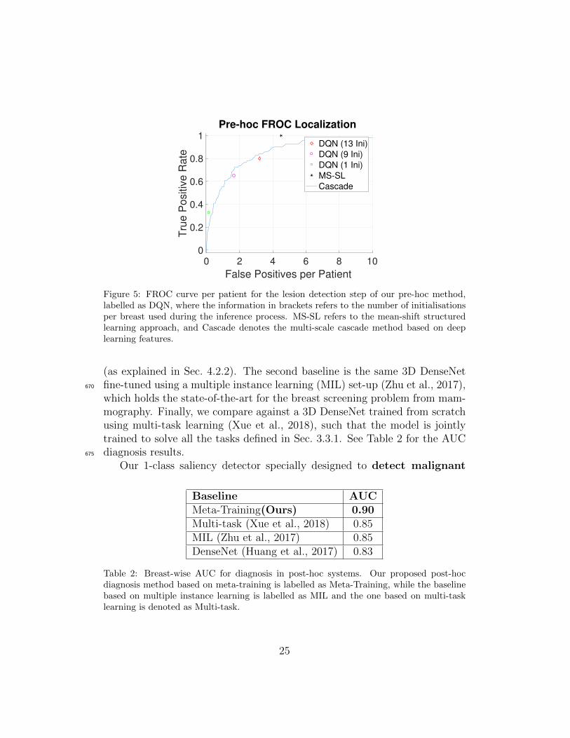
on deep learning features (Maicas et al., 2017a), and a mean-shift clusteringmethod followed by structured learning (McClymont et al., 2014) (note thatonly one operating point is available for this approach), which is evaluatedon the same dataset using a different training and testing data split. Figure 5shows the FROC curve with the detection results and Table 1 contains the660

inference times per patient needed by each of the methods.The diagnosis of breast volumes, based on the classification of the de-

tected regions, achieves an AUC of 0.85, if all volumes in the test dataset areconsidered.

4.2.5. Experimental Results for the Post-hoc System665

We evaluate the performance of our post-hoc diagnosis against threestate-of-the-art classifiers. The first baseline is the 3D DenseNet (Huanget al., 2017) that has been optimized to solve the breast screening problem

24

0 2 4 6 8 10

False Positives per Patient

0

0.2

0.4

0.6

0.8

1

Tru

e P

ositiv

e R

ate

Pre-hoc FROC Localization

DQN (13 Ini)

DQN (9 Ini)

DQN (1 Ini)

MS-SL

Cascade

Figure 5: FROC curve per patient for the lesion detection step of our pre-hoc method,labelled as DQN, where the information in brackets refers to the number of initialisationsper breast used during the inference process. MS-SL refers to the mean-shift structuredlearning approach, and Cascade denotes the multi-scale cascade method based on deeplearning features.

(as explained in Sec. 4.2.2). The second baseline is the same 3D DenseNetfine-tuned using a multiple instance learning (MIL) set-up (Zhu et al., 2017),670

which holds the state-of-the-art for the breast screening problem from mam-mography. Finally, we compare against a 3D DenseNet trained from scratchusing multi-task learning (Xue et al., 2018), such that the model is jointlytrained to solve all the tasks defined in Sec. 3.3.1. See Table 2 for the AUCdiagnosis results.675

Our 1-class saliency detector specially designed to detect malignant

Baseline AUCMeta-Training(Ours) 0.90Multi-task (Xue et al., 2018) 0.85MIL (Zhu et al., 2017) 0.85DenseNet (Huang et al., 2017) 0.83

Table 2: Breast-wise AUC for diagnosis in post-hoc systems. Our proposed post-hocdiagnosis method based on meta-training is labelled as Meta-Training, while the baselinebased on multiple instance learning is labelled as MIL and the one based on multi-tasklearning is denoted as Multi-task.

25

lesions in positively classified volumes is compared against the followingbaselines: CAM (Zhou et al., 2016), and Grad-CAM and Guided Grad-CAM (Selvaraju et al., 2017). Figure 6 shows the FROC curves for ourproposed methods and baselines in each of the two scenarios (A) and (+).680

0 2 4 6 8 10

False Positives per Patient

0

0.2

0.4

0.6

0.8

1

Tru

e P

ositiv

e R

ate

Post-hoc FROC Localization

1-Class Saliency (A)

1-Class Saliency (+)

Guided-Grad-CAM (A)

Guided-Grad-CAM (+)

Grad-CAM (A)

Grad-CAM (+)

CAM (A)

CAM (+)

Figure 6: Patient-wise FROC curves for post-hoc malignant lesion detection, where ourmethod is denoted as 1-Class Saliency. Baselines are denoted as CAM (Zhou et al., 2016),and Grad-CAM and Guided Grad-CAM (Selvaraju et al., 2017). For each method, wepresent two scenarios: (A) all the volumes in the test set are considered to compute theFROC, and (+) only positively classified volumes are considered.

4.2.6. Experimental Results for the Comparison Between Pre- and Post-Hoc

Table 3 contains the AUC for the malignancy diagnosis measured breast-wise and patient-wise for the pre-hoc and post-hoc approaches. Figure 7shows the ROC curves used in the computation of the AUC in Table 3.Figure 8 shows the FROC curves for malignant lesion detection of pre-hoc and685

post-hoc ( (A) and (+) ) methods. Figures 9, 10, and 11 display examples ofbreast diagnosis and lesion localizations obtained from the proposed pre-hocand post-hoc methods, where both methods correctly performed diagnosis(Fig. 9), only the pre-hoc method correctly diagnosed the breast (Fig. 10),and only the post-hoc method correctly diagnosed the breast (Fig. 11).690

5. Discussion

The localization step in the pre-hoc method achieves similar accuracy tothe baseline methods. As shown in Figure 5, the TPR and FPP directly

26

Pre-Hoc Post-HocBreast-wise 0.85± 0.04 0.90± 0.04Patient-wise 0.81± 0.05 0.91± 0.04

Table 3: AUC comparing the diagnosis performance between pre-hoc and post-hoc mea-sured breast-wise and patient-wise.

0 0.2 0.4 0.6 0.8 1

False Positive Rate

0

0.2

0.4

0.6

0.8

1

Tru

e P

ositiv

e R

ate

Full Pipeline ROC Diagnosis

Post-hoc Patient Wise

Post-hoc Breast Wise

Pre-hoc Patient Wise

Pre-hoc Breast Wise

Figure 7: ROC curves for malignancy diagnosis of pre-hoc and post-hoc full pipelinesmeasures breast and patient-wise. See Table 3 for the AUCs and estimated error.

depends on the number of initializations used by the reinforcement learningalgorithm. In addition, the performance of our localization step is very simi-695

lar to the baseline based on a multi-scale cascade using exhaustive search withdeep features. However, multi-scale cascade (164s) and clustering+structurelearning (several hours) methods require large inference times compared toour attention model (92s) as shown in Table 1.

The post-hoc diagnosis step improves over several baseline methods, as700

shown in Table 2. These baseline methods are based on a DenseNet (Huanget al., 2017), specifically optimised for the breast screening classification,and on extensions derived from multiple instance learning (Zhu et al., 2017)and multi-task learning (Xue et al., 2018). These results show that meta-training the model to solve tasks with small training sets is an important step705

to improve the learning of methods when only small datasets are available.Baseline approaches (Huang et al., 2017; Xue et al., 2018) only show a limitedimprovement over the DenseNet baseline.

27

0 1 2 3 4 5

False Positives per Patient

0

0.2

0.4

0.6

0.8

1

Tru

e P

ositiv

e R

ate

Full Pipeline FROC Localization

Pre-hoc

Post-hoc (A)

Post-hoc (+)

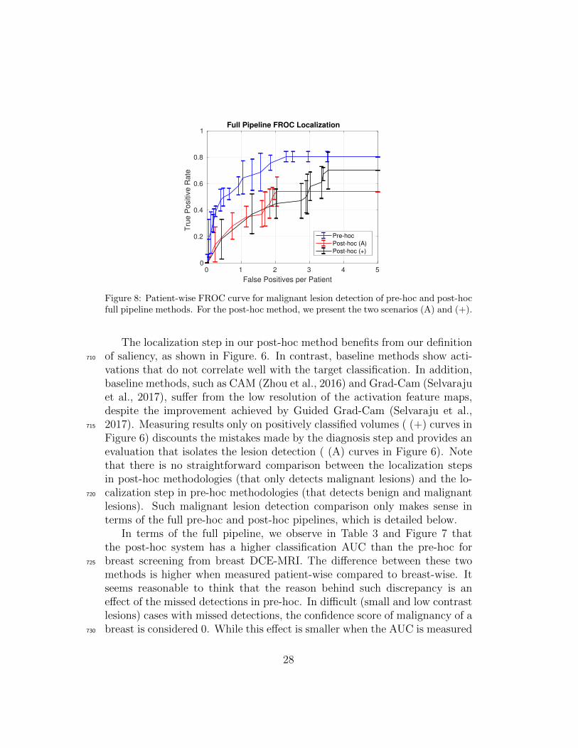
Figure 8: Patient-wise FROC curve for malignant lesion detection of pre-hoc and post-hocfull pipeline methods. For the post-hoc method, we present the two scenarios (A) and (+).

The localization step in our post-hoc method benefits from our definitionof saliency, as shown in Figure. 6. In contrast, baseline methods show acti-710

vations that do not correlate well with the target classification. In addition,baseline methods, such as CAM (Zhou et al., 2016) and Grad-Cam (Selvarajuet al., 2017), suffer from the low resolution of the activation feature maps,despite the improvement achieved by Guided Grad-Cam (Selvaraju et al.,2017). Measuring results only on positively classified volumes ( (+) curves in715

Figure 6) discounts the mistakes made by the diagnosis step and provides anevaluation that isolates the lesion detection ( (A) curves in Figure 6). Notethat there is no straightforward comparison between the localization stepsin post-hoc methodologies (that only detects malignant lesions) and the lo-calization step in pre-hoc methodologies (that detects benign and malignant720

lesions). Such malignant lesion detection comparison only makes sense interms of the full pre-hoc and post-hoc pipelines, which is detailed below.

In terms of the full pipeline, we observe in Table 3 and Figure 7 thatthe post-hoc system has a higher classification AUC than the pre-hoc forbreast screening from breast DCE-MRI. The difference between these two725

methods is higher when measured patient-wise compared to breast-wise. Itseems reasonable to think that the reason behind such discrepancy is aneffect of the missed detections in pre-hoc. In difficult (small and low contrastlesions) cases with missed detections, the confidence score of malignancy of abreast is considered 0. While this effect is smaller when the AUC is measured730

28

(a) (b) (c)

(d) (e) (f)

Figure 9: Example of two correct diagnosis by both pre-hoc and post-hoc full pipelinemethods. Left column is the ground truth, middle column is the result of the pre-hocmethod and right column is the result of the post-hoc method. Red image frames indicatemalignant diagnosis, green frames indicate non-malignant diagnosis. Detections in redindicates TP malignant detections, yellow detections indicate FP malignant detections,detections in green indicate benign lesions. First row: pre-hoc and post-hoc correctpositive diagnosis with the malignant lesion detected. Second row: pre-hoc and post-hoc correct negative diagnosis where the pre-hoc method correctly classified as negative adetected benign lesion and the post-hoc method did not localize any malignant lesion.

breast-wise (as there are 118 samples of breasts), it is larger when measuredpatient-wise (59 samples of patients). Furthermore, the better results ofthe post-hoc method suggest that the analysis of the whole image allowsit to find indications for malignancy that are located in other areas of theimage (Kostopoulos et al., 2017).735

Regarding the localization of malignant lesions, the pre-hoc system achievesbetter accuracy, compared with the post-hoc. This suggests that the strongannotations used to train the pre-hoc method gives it an advantage for thelocalisation of lesions, when compared with the weak annotation used to trainthe post-hoc approach. This issue is exemplified in Figure 9 (Row 1), where740

although both approaches present a correct diagnosis, the post-hoc methodyields a higher number of false positive malignant lesion detections. A simi-

29

(a) (b) (c)

(d) (e) (f)

Figure 10: Example of two correct diagnosis by the pre-hoc system, but wrongly diagnosedby the post-hoc method. Left column is the ground truth, middle column is the result of thepre-hoc method and right column is the result of the post-hoc method. Red image framesindicate malignant diagnosis, green frames indicate non-malignant diagnosis. Detections inred indicate TP malignant detections, yellow detections indicate FP malignant detections,detection in blue indicates a ROI detection correctly classified as negative (non-malignant).First row: correct positive diagnosis by the pre-hoc method with the malignant lesioncorrectly detected but incorrect non-malignant diagnosis by the post-hoc method. Secondrow: correct negative diagnosis by the pre-hoc method, but incorrect positive diagnosisby the post-hoc system – yielding the potential malignant regions in the rectangles shownin yellow.

lar behaviour can be seen in Figure 10 (Row 2), where the post-hoc producesan incorrect diagnosis and additionally yields two false positive detections.In addition, the detection step for the pre-hoc system is mainly designed to745

achieve good performance when only a small training set is available. On thecontrary, the malignant lesion localization step in the post-hoc approach isnot particularly focused on being able to perform well from a small dataset.This difference in design focus is likely to be influencing the detection resultstoo. Finally, it is worth noting that the FROC for the post-hoc approach750

(Post-hoc (A) curve in Fig. 8) is affected by the diagnosis process. However,if we remove the effect of the diagnosis step and consider the performanceof malignant lesion localization in positively classified volumes, we observe acloser performance compared to the pre-hoc method, even though the post-

30

(a) (b) (c)

(d) (e) (f)

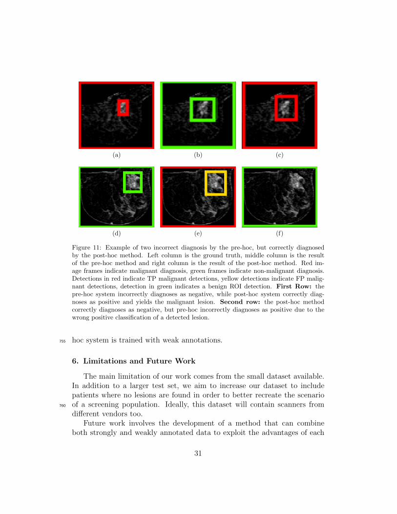
Figure 11: Example of two incorrect diagnosis by the pre-hoc, but correctly diagnosedby the post-hoc method. Left column is the ground truth, middle column is the resultof the pre-hoc method and right column is the result of the post-hoc method. Red im-age frames indicate malignant diagnosis, green frames indicate non-malignant diagnosis.Detections in red indicate TP malignant detections, yellow detections indicate FP malig-nant detections, detection in green indicates a benign ROI detection. First Row: thepre-hoc system incorrectly diagnoses as negative, while post-hoc system correctly diag-noses as positive and yields the malignant lesion. Second row: the post-hoc methodcorrectly diagnoses as negative, but pre-hoc incorrectly diagnoses as positive due to thewrong positive classification of a detected lesion.

hoc system is trained with weak annotations.755

6. Limitations and Future Work

The main limitation of our work comes from the small dataset available.In addition to a larger test set, we aim to increase our dataset to includepatients where no lesions are found in order to better recreate the scenarioof a screening population. Ideally, this dataset will contain scanners from760

different vendors too.Future work involves the development of a method that can combine

both strongly and weakly annotated data to exploit the advantages of each

31

approach for lesion detection and diagnosis. We will also focus on the im-provement of the malignant lesion localization in post-hoc methodologies by765

designing a new method specifically for the small training set available. Webelieve that the lesion localization step in pre-hoc approaches could also beimproved in terms of inference time by running the different initializations ofthe detection algorithm in parallel and by optimizing the resizing operationof the current bounding volume (Maicas et al., 2017b). In addition, the use770

of a U-net (Ronneberger et al., 2015) would allow the implementation of afaster segmentation map maintaining the detection accuracy. We also planto extend the diagnosis stage of the pre-hoc method by building a classifierthat is trained similarly to the proposed for the diagnosis step of the post-hoc approach. Finally, it would be interesting to design a method that could775

diagnose based on the combined analysis of MRI and mammography.

7. Conclusion

We introduced and compared two different approaches for breast screen-ing from breast DCE-MRI: pre-hoc and post-hoc methods. The pre-hocmethod localizes suspicious regions (benign and malignant lesions) using an780

attention model based on deep reinforcement learning. Detected regionswere subsequently classified into malignant or non-malignant lesions usinga 3D DenseNet. The post-hoc method diagnoses a DCE-MRI breast vol-ume using a classifier that, before being trained to solve the breast screeningtask, has been meta-trained to solve several breast-related tasks where only785

small training sets are available. Malignant regions are then localized with a1-class saliency detector specifically designed for post-hoc systems that per-form diagnosis. Results showed that the post-hoc method can achieve betterperformance for malignancy diagnosis, whereas the pre-hoc method couldmore precisely localize malignant lesions. However, this improvement of the790

pre-hoc detection method relies on the employment of strong annotationsduring the training process. On the other hand, post-hoc methods only useweak labels during the training phase and outperforms pre-hoc methods indiagnosis, which is the main aim of a breast screening system. In conclu-sion, we believe that future research should focus on the development and795

improvement of post-hoc diagnosis methods.

32

References

Agner, S.C., Rosen, M.A., Englander, S., Tomaszewski, J.E., Feldman, M.D.,Zhang, P., Mies, C., Schnall, M.D., Madabhushi, A., 2014. Computerizedimage analysis for identifying triple-negative breast cancers and differen-800

tiating them from other molecular subtypes of breast cancer on dynamiccontrast-enhanced mr images: a feasibility study. Radiology 272, 91–99.

AIHW, 2007. Cancer in Australia 2017. Technical Report. The AustralianInstitute of Health and Welfare.

Amit, G., Ben-Ari, R., Hadad, O., Monovich, E., Granot, N., Hashoul,805

S., 2017a. Classification of breast mri lesions using small-size trainingsets: comparison of deep learning approaches, in: Medical Imaging 2017:Computer-Aided Diagnosis, International Society for Optics and Photon-ics. p. 101341H.

Amit, G., Hadad, O., Alpert, S., Tlusty, T., Gur, Y., Ben-Ari, R., Hashoul,810

S., 2017b. Hybrid mass detection in breast mri combining unsupervisedsaliency analysis and deep learning, in: International Conference on Med-ical Image Computing and Computer-Assisted Intervention, Springer. pp.594–602.

Behrens, S., Laue, H., Althaus, M., Boehler, T., Kuemmerlen, B., Hahn,815

H.K., Peitgen, H.O., 2007. Computer assistance for mr based diagnosisof breast cancer: present and future challenges. Computerized medicalimaging and graphics 31, 236–247.

Bishop, C.M., 2006. Pattern recognition and machine learning. springer.

Bradley, A.P., 1997. The use of the area under the roc curve in the evaluation820

of machine learning algorithms. Pattern recognition 30, 1145–1159.

Caicedo, J.C., Lazebnik, S., 2015. Active object localization with deep rein-forcement learning, in: Proceedings of the IEEE International Conferenceon Computer Vision, pp. 2488–2496.

Caruana, R., Lou, Y., Gehrke, J., Koch, P., Sturm, M., Elhadad, N., 2015.825

Intelligible models for healthcare: Predicting pneumonia risk and hospital30-day readmission, in: Proceedings of the 21th ACM SIGKDD Interna-tional Conference on Knowledge Discovery and Data Mining, ACM. pp.1721–1730.

33

Chen, W., Giger, M.L., Bick, U., 2006. A fuzzy c-means (fcm)-based830

approach for computerized segmentation of breast lesions in dynamiccontrast-enhanced mr images. Academic radiology 13, 63–72.

Dalmıs, M.U., Gubern-Merida, A., Vreemann, S., Karssemeijer, N., Mann,R., Platel, B., 2016. A computer-aided diagnosis system for breast dce-mriat high spatiotemporal resolution. Medical physics 43, 84–94.835

Dalmıs, M.U., Vreemann, S., Kooi, T., Mann, R.M., Karssemeijer, N.,Gubern-Merida, A., 2018. Fully automated detection of breast cancerin screening mri using convolutional neural networks. Journal of MedicalImaging 5, 014502.

DeSantis, C.E., Bray, F., Ferlay, J., Lortet-Tieulent, J., Anderson, B.O.,840

Jemal, A., 2015. International variation in female breast cancer incidenceand mortality rates. Cancer Epidemiology and Prevention Biomarkers 24,1495–1506.

Dhungel, N., Carneiro, G., Bradley, A.P., 2015. Automated mass detectionin mammograms using cascaded deep learning and random forests, in:845

2015 international conference on digital image computing: techniques andapplications (DICTA), IEEE. pp. 1–8.

Dubost, F., Bortsova, G., Adams, H., Ikram, A., Niessen, W.J., Vernooij, M.,De Bruijne, M., 2017. Gp-unet: Lesion detection from weak labels witha 3d regression network, in: International Conference on Medical Image850

Computing and Computer-Assisted Intervention, Springer. pp. 214–221.

Esteva, A., Kuprel, B., Novoa, R.A., Ko, J., Swetter, S.M., Blau, H.M.,Thrun, S., 2017. Dermatologist-level classification of skin cancer with deepneural networks. Nature 542, 115.

Feng, X., Yang, J., Laine, A.F., Angelini, E.D., 2017. Discriminative local-855

ization in cnns for weakly-supervised segmentation of pulmonary nodules,in: International Conference on Medical Image Computing and Computer-Assisted Intervention, Springer. pp. 568–576.

Gallego-Ortiz, C., Martel, A.L., 2015. Improving the accuracy of computer-aided diagnosis for breast mr imaging by differentiating between mass and860

nonmass lesions. Radiology 278, 679–688.

34

Gilbert, F., Selamoglu, A., 2018. Personalised screening: is this the wayforward? Clinical radiology 73, 327–333.

Grimm, L.J., Anderson, A.L., Baker, J.A., Johnson, K.S., Walsh, R., Yoon,S.C., Ghate, S.V., 2015. Interobserver variability between breast imagers865

using the fifth edition of the bi-rads mri lexicon. American Journal ofRoentgenology 204, 1120–1124.

Gubern-Merida, A., Martı, R., Melendez, J., Hauth, J.L., Mann, R.M.,Karssemeijer, N., Platel, B., 2015. Automated localization of breast cancerin dce-mri. Medical image analysis 20, 265–274.870

Gubern-Merida, A., Vreemann, S., Martı, R., Melendez, J., Lardenoije, S.,Mann, R.M., Karssemeijer, N., Platel, B., 2016. Automated detectionof breast cancer in false-negative screening mri studies from women atincreased risk. European journal of radiology 85, 472–479.

Hanley, J.A., McNeil, B.J., 1983. A method of comparing the areas un-875

der receiver operating characteristic curves derived from the same cases.Radiology 148, 839–843.

Hayton, P., Brady, M., Tarassenko, L., Moore, N., 1997. Analysis of dynamicmr breast images using a model of contrast enhancement. Medical imageanalysis 1, 207–224.880

He, K., Gkioxari, G., Dollar, P., Girshick, R., 2017. Mask r-cnn, in: Com-puter Vision (ICCV), 2017 IEEE International Conference on, IEEE. pp.2980–2988.

He, K., Zhang, X., Ren, S., Sun, J., 2016. Deep residual learning for imagerecognition, in: Proceedings of the IEEE conference on computer vision885

and pattern recognition, pp. 770–778.

Huang, G., Liu, Z., van der Maaten, L., Weinberger, K.Q., 2017. Denselyconnected convolutional networks, in: Proceedings of the IEEE Conferenceon Computer Vision and Pattern Recognition, pp. 4700–4708.

Huang, G., Sun, Y., Liu, Z., Sedra, D., Weinberger, K.Q., 2016. Deep net-890

works with stochastic depth, in: European Conference on Computer Vi-sion, Springer. pp. 646–661.

35

Kingma, D., Ba, J., 2014. Adam: A method for stochastic optimization.arXiv preprint arXiv:1412.6980 .

Kostopoulos, S.A., Vassiou, K.G., Lavdas, E.N., Cavouras, D.A., Kalatzis,895

I.K., Asvestas, P.A., Arvanitis, D.L., Fezoulidis, I.V., Glotsos, D.T., 2017.Computer-based automated estimation of breast vascularity and correla-tion with breast cancer in dce-mri images. Magnetic resonance imaging35, 39–45.

Kousi, E., Borri, M., Dean, J., Panek, R., Scurr, E., Leach, M.O., Schmidt,900

M.A., 2015. Quality assurance in mri breast screening: comparing signal-to-noise ratio in dynamic contrast-enhanced imaging protocols. Physics inMedicine & Biology 61, 37.

Kriege, M., Brekelmans, C.T., Boetes, C., Besnard, P.E., Zonderland, H.M.,Obdeijn, I.M., Manoliu, R.A., Kok, T., Peterse, H., Tilanus-Linthorst,905

M.M., et al., 2004. Efficacy of mri and mammography for breast-cancerscreening in women with a familial or genetic predisposition. New EnglandJournal of Medicine 351, 427–437.

Krizhevsky, A., Sutskever, I., Hinton, G.E., 2012. Imagenet classificationwith deep convolutional neural networks, in: Advances in neural informa-910

tion processing systems, pp. 1097–1105.

Lee, K.A., Talati, N., Oudsema, R., Steinberger, S., Margolies, L.R., 2018.Bi-rads 3: current and future use of probably benign. Current radiologyreports 6, 5.

Lehman, C.D., Blume, J.D., DeMartini, W.B., Hylton, N.M., Herman, B.,915

Schnall, M.D., 2013. Accuracy and interpretation time of computer-aideddetection among novice and experienced breast mri readers. AmericanJournal of Roentgenology 200, W683–W689.

Levman, J.E., Causer, P., Warner, E., Martel, A.L., 2009. Effect of theenhancement threshold on the computer-aided detection of breast cancer920

using mri. Academic radiology 16, 1064–1069.

Li, Z., Wang, C., Han, M., Xue, Y., Wei, W., Li, L.J., Fei-Fei, L., 2018.Thoracic disease identification and localization with limited supervision,in: Proceedings of the IEEE Conference on Computer Vision and PatternRecognition, pp. 8290–8299.925

36

Liu, H., Zheng, Y., Liang, D., Tang, P., Ren, F., Zhang, L., Zhao, Z., 2017.Total variation based dce-mri decomposition by separating lesion frombackground for time-intensity curve estimation. Medical physics 44, 2321–2331.

Maicas, G., Bradley, A.P., Nascimento, J.C., Reid, I., Carneiro, G., 2018.930

Training medical image analysis systems like radiologists, in: MedicalImage Computing and Computer Assisted Intervention – MICCAI 2018,Springer International Publishing, Cham. pp. 546–554.

Maicas, G., Carneiro, G., Bradley, A.P., 2017a. Globally optimal breast masssegmentation from dce-mri using deep semantic segmentation as shape935

prior, in: 2017 IEEE 14th International Symposium on Biomedical Imaging(ISBI 2017), pp. 305–309.

Maicas, G., Carneiro, G., Bradley, A.P., Nascimento, J.C., Reid, I., 2017b.Deep reinforcement learning for active breast lesion detection from dce-mri, in: Medical Image Computing and Computer-Assisted Intervention940

MICCAI 2017, Springer International Publishing, Cham. pp. 665–673.

Maicas, G., Snaauw, G., Bradley, A.P., Reid, I., Carneiro, G., 2019. Modelagnostic saliency for weakly supervised lesion detection from breast dce-mri, in: 2019 IEEE 16th International Symposium on Biomedical Imaging(ISBI 2019), pp. 1057–1060.945

Mainiero, M.B., Moy, L., Baron, P., Didwania, A.D., Green, E.D., Heller,S.L., Holbrook, A.I., Lee, S.J., Lewin, A.A., Lourenco, A.P., et al., 2017.Acr appropriateness criteria R© breast cancer screening. Journal of theAmerican College of Radiology 14, S383–S390.

Mango, V.L., Morris, E.A., Dershaw, D.D., Abramson, A., Fry, C.,950

Moskowitz, C.S., Hughes, M., Kaplan, J., Jochelson, M.S., 2015. Abbre-viated protocol for breast mri: are multiple sequences needed for cancerdetection? European journal of radiology 84, 65–70.

Matiisen, T., Oliver, A., Cohen, T., Schulman, J., 2017. Teacher-studentcurriculum learning. arXiv preprint arXiv:1707.00183 .955

Mcclymont, D., 2015. Computer assisted detection and characterisation ofbreast cancer in MRI. Ph.D. thesis.

37

McClymont, D., Mehnert, A., Trakic, A., et al., 2014. Fully automatic lesionsegmentation in breast MRI using mean-shift and graph-cuts on a regionadjacency graph. JMRI 39, 795–804.960

Meinel, L.A., Stolpen, A.H., Berbaum, K.S., Fajardo, L.L., Reinhardt, J.M.,2007. Breast mri lesion classification: Improved performance of humanreaders with a backpropagation neural network computer-aided diagnosis(cad) system. Journal of magnetic resonance imaging 25, 89–95.

Milenkovic, J., Dalmıs, M.U., Zgajnar, J., Platel, B., 2017. Textural analysis965

of early-phase spatiotemporal changes in contrast enhancement of breastlesions imaged with an ultrafast dce-mri protocol. Medical physics 44,4652–4664.

Mnih, V., Kavukcuoglu, K., Silver, D., Rusu, A.A., Veness, J., Bellemare,M.G., Graves, A., Riedmiller, M., Fidjeland, A.K., Ostrovski, G., et al.,970

2015. Human-level control through deep reinforcement learning. Nature518, 529.

Mus, R.D., Borelli, C., Bult, P., Weiland, E., Karssemeijer, N., Barentsz,J.O., Gubern-Merida, A., Platel, B., Mann, R.M., 2017. Time to enhance-ment derived from ultrafast breast mri as a novel parameter to discriminate975

benign from malignant breast lesions. European journal of radiology 89,90–96.

Platel, B., Mus, R., Welte, T., Karssemeijer, N., Mann, R., 2014. Automatedcharacterization of breast lesions imaged with an ultrafast dce-mr protocol.IEEE transactions on medical imaging 33, 225–232.980

Rasti, R., Teshnehlab, M., Phung, S.L., 2017. Breast cancer diagnosis indce-mri using mixture ensemble of convolutional neural networks. PatternRecognition 72, 381–390.

Ren, S., He, K., Girshick, R., Sun, J., 2015. Faster r-cnn: Towards real-timeobject detection with region proposal networks, in: Advances in neural985

information processing systems, pp. 91–99.

Renz, D.M., Bottcher, J., Diekmann, F., Poellinger, A., Maurer, M.H., Pfeil,A., Streitparth, F., Collettini, F., Bick, U., Hamm, B., et al., 2012. Detec-tion and classification of contrast-enhancing masses by a fully automatic

38

computer-assisted diagnosis system for breast mri. Journal of Magnetic990

Resonance Imaging 35, 1077–1088.

Ribli, D., Horvath, A., Unger, Z., Pollner, P., Csabai, I., 2018. Detecting andclassifying lesions in mammograms with deep learning. Scientific reports8, 4165.

Ronneberger, O., Fischer, P., Brox, T., 2015. U-net: Convolutional networks995

for biomedical image segmentation, in: International Conference on Med-ical image computing and computer-assisted intervention, Springer. pp.234–241.

Saadatmand, S., Bretveld, R., Siesling, S., Tilanus-Linthorst, M.M., 2015.Influence of tumour stage at breast cancer detection on survival in modern1000

times: population based study in 173 797 patients. Bmj 351, h4901.

Selvaraju, R.R., Cogswell, M., Das, A., Vedantam, R., Parikh, D., Batra, D.,2017. Grad-cam: Visual explanations from deep networks via gradient-based localization, in: Computer Vision (ICCV), 2017 IEEE InternationalConference on, IEEE. pp. 618–626.1005

Shimauchi, A., Giger, M.L., Bhooshan, N., Lan, L., Pesce, L.L., Lee, J.K.,Abe, H., Newstead, G.M., 2011. Evaluation of clinical breast mr imagingperformed with prototype computer-aided diagnosis breast mr imagingworkstation: reader study. Radiology 258, 696–704.

Siegel, R.L., Miller, K.D., Jemal, A., 2017. Cancer statistics, 2017. CA: A1010

Cancer Journal for Clinicians .

Smith, R.A., Andrews, K.S., Brooks, D., Fedewa, S.A., Manassaram-Baptiste, D., Saslow, D., Brawley, O.W., Wender, R.C., 2017. Cancerscreening in the united states, 2017: a review of current american cancersociety guidelines and current issues in cancer screening. CA: a cancer1015

journal for clinicians 67, 100–121.

Soares, F., Janela, F., Pereira, M., Seabra, J., Freire, M.M., 2013. 3d lacu-narity in multifractal analysis of breast tumor lesions in dynamic contrast-enhanced magnetic resonance imaging. IEEE Transactions on Image Pro-cessing 22, 4422–4435.1020

39

Song, J.L., Chen, C., Yuan, J.P., Sun, S.R., 2016. Progress in the clinicaldetection of heterogeneity in breast cancer. Cancer medicine 5, 3475–3488.

Sutton, R., Barto, A.G., 1998. Reinforcement learning: An introduction.volume 2. MIT press.

Tajbakhsh, N., Shin, J.Y., Gurudu, S.R., Hurst, R.T., Kendall, C.B., Got-1025

way, M.B., Liang, J., 2016. Convolutional neural networks for medicalimage analysis: Full training or fine tuning? IEEE transactions on medi-cal imaging 35, 1299–1312.

Torre, L.A., Bray, F., Siegel, R.L., Ferlay, J., Lortet-Tieulent, J., Jemal, A.,2015. Global cancer statistics, 2012. CA: a cancer journal for clinicians1030

65, 87–108.

Vreemann, S., Gubern-Merida, A., Lardenoije, S., Bult, P., Karssemeijer, N.,Pinker, K., Mann, R.M., 2018. The frequency of missed breast cancers inwomen participating in a high-risk mri screening program. Breast CancerResearch and Treatment .1035

Wang, L., Harz, M., Boehler, T., Platel, B., Homeyer, A., Hahn, H.K.,2014. A robust and extendable framework towards fully automated diag-nosis of nonmass lesions in breast dce-mri, in: International Symposiumon Biomedical Imaging, IEEE. pp. 129–132.

Wang, X., Peng, Y., Lu, L., Lu, Z., Bagheri, M., Summers, R.M., 2017a.1040

Chestx-ray8: Hospital-scale chest x-ray database and benchmarks onweakly-supervised classification and localization of common thorax dis-eases, in: Proceedings of the IEEE conference on computer vision andpattern recognition, pp. 2097–2106.

Wang, Z., Yin, Y., Shi, J., Fang, W., Li, H., Wang, X., 2017b. Zoom-in-net:1045

Deep mining lesions for diabetic retinopathy detection, in: InternationalConference on Medical Image Computing and Computer-Assisted Inter-vention, Springer. pp. 267–275.

Welch, H.G., Prorok, P.C., OMalley, A.J., Kramer, B.S., 2016. Breast-cancertumor size, overdiagnosis, and mammography screening effectiveness. New1050

England Journal of Medicine 375, 1438–1447.

40

Wood, C., 2005. Computer aided detection (cad) for breast mri. Technologyin cancer research & treatment 4, 49–53.

Xue, W., Brahm, G., Pandey, S., Leung, S., Li, S., 2018. Full left ventriclequantification via deep multitask relationships learning. Medical image1055

analysis 43, 54–65.

Yang, X., Wang, Z., Liu, C., Le, H.M., Chen, J., Cheng, K.T.T., Wang, L.,2017. Joint detection and diagnosis of prostate cancer in multi-parametricmri based on multimodal convolutional neural networks, in: InternationalConference on Medical Image Computing and Computer-Assisted Inter-1060

vention, Springer. pp. 426–434.

Zeiler, M.D., Fergus, R., 2014. Visualizing and understanding convolutionalnetworks, in: European conference on computer vision, Springer. pp. 818–833.

Zhou, B., Khosla, A., Lapedriza, A., Oliva, A., Torralba, A., 2016. Learning1065

deep features for discriminative localization, in: Proceedings of the IEEEConference on Computer Vision and Pattern Recognition, pp. 2921–2929.

Zhu, W., Lou, Q., Vang, Y.S., Xie, X., 2017. Deep multi-instance net-works with sparse label assignment for whole mammogram classification,in: International Conference on Medical Image Computing and Computer-1070

Assisted Intervention, Springer. pp. 603–611.

41