practical work with g4 - lip

Practical work with G4

E. Chabert

E. Conte

ESIPAP computing session 2017 – E. Chabert, E. Conte Slide 2 / 55

Skills to acquire


• Building an official Geant4 example

• Using one of the possible GUI (Graphics User Interface)

• Using the user guide & Doxygen documentation of Geant4

• Understanding the structure of a Geant4 program

• Modifying the detector description

• Running the simulation

• Accessing produced data


Outlines


user developer


Outlines


1. Setting your environment

2. Building a G4 example

3. Running example B4a

4. Studying the simulation in example B4a

5. Analyzing and editing the main function

6. Analyzing and editing the detector description

7. Analyzing and editing the action description


Outlines


Disclaimers


1. Setting your setup


1. Setting your environment




Accessing the Linux virtual machine


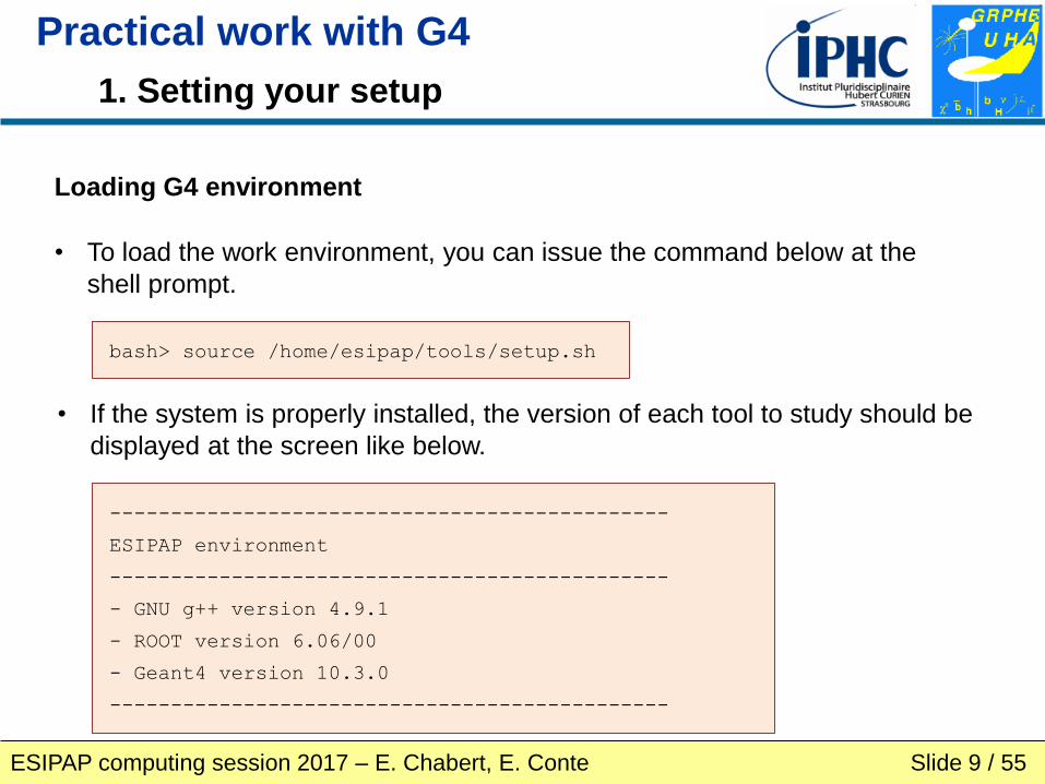
Loading G4 environment

bash> source /home/esipap/tools/setup.sh

----------------------------------------------

ESIPAP environment

----------------------------------------------

- GNU g++ version 4.9.1

- ROOT version 6.06/00

- Geant4 version 10.3.0

----------------------------------------------

• To load the work environment, you can issue the command below at the

shell prompt.

• If the system is properly installed, the version of each tool to study should be

displayed at the screen like below.






Checking that G4 environment is properly loaded

bash> geant4-config --version

• If your setup is properly loaded, you should call the gean4-config

program whatever the folder where you are. This program provides

some useful information.

• For example, displaying the release version of the Geant 4 program

installed on your system:




Are the physics datasets installed?

bash> geant4-config --check-datasets

• Geant4 needs physics datasets which must be downloaded from the

official website. As these datasets are heavy, it is possible that all of

them are not installed on your system.

• To enumerate the list of the datasets installed on your system, type the

following command line.




What are the GUI installed on your system?

• Geant4 requires one graphical package for visualization.

There are several possible packages:

• OpenGL (OGL)

• Qt

• OpenInventor

• RayTracer

• ASCIITree

• Wt

• HepRep

• DAWN

• VRML

• gMocren




What are the GUI installed on your system?

bash> geant4-config --has-feature opengl-x11

• In this tutorial, we use the OpenGL (or « OGL » in G4 language)

package.

• Check with geant4-config that this package is installed.


2. Building an example






Choosing an example



Choosing an example


• 3 categories of examples

• Selecting « Basic Examples » B4



Choosing an example


• There are 4

variants of the

B4 example:

B4a, B4b,

B4c & B4d.

• Focusing

only on B4a.



Choosing an example


• What kind of apparatus does the

B4a example describe?

• Which physis datasets are

required? Are they installed on

your system?

To do




Copying a G4 example

bash> ls /home/esipap/tools/geant4.10.03/share/Geant4-10.3.0/examples

• Finding where are stored the Geant4 example.

On the ESIPAP computers, you have to issue the following command:

• Copying the folder related to the B4a example into your home folder:

bash> cp –rv /home/esipap/tools/geant4.10.03/share/Geant4- \

10.3.0/examples/basic/B4/B4a ./




Building with cMake

bash> make B4a_build

bash> cd B4a_build

bash> cmake ../B4a

bash> make

• Creating, in your home folder, a folder devoted to the building of the

example. In this tutorial, this folder will be called « B4a_build »:

• Launching the CMake program for generating automatically a Makefile:

• Building the example with GNU Make:




What is cMake?

CMakeLists.txt

Makefile

for GNU Make

*.sln

for Visual Studio

CMake


3. Running the example






Executing the example

bash> ./exampleB4

• In the B4a_build folder, if the building is successful,

you must find the executable file « exampleB4 ».

• Issue the command line to execute the program.




Executing the example

2 windows are opened!!!




Using the prompt

In the text console, you can type some commands.

2 main commands to know:

Idle> exit

• Exit the program

Idle> help

• Listing the possible commands and see their syntax

Using numbers for selecting an item




Using the prompt

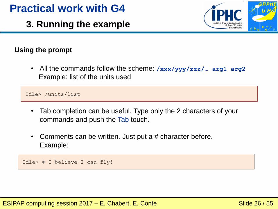
• All the commands follow the scheme: /xxx/yyy/zzz/… arg1 arg2

Example: list of the units used

• Tab completion can be useful. Type only the 2 characters of your

commands and push the Tab touch.

• Comments can be written. Just put a # character before.

Example:

Idle> # I believe I can fly!

Idle> /units/list




Using the prompt

• It is also possible to access to the value of parameters.

Just put a ? character before the command.

Example:

Idle> ?/gun/particle




Visualization commands

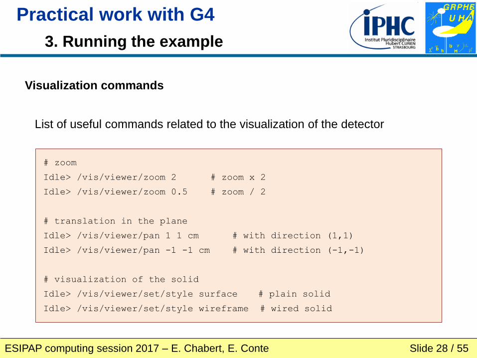
List of useful commands related to the visualization of the detector

# zoom

Idle> /vis/viewer/zoom 2 # zoom x 2

Idle> /vis/viewer/zoom 0.5 # zoom / 2

# translation in the plane

Idle> /vis/viewer/pan 1 1 cm # with direction (1,1)

Idle> /vis/viewer/pan -1 -1 cm # with direction (-1,-1)

# visualization of the solid

Idle> /vis/viewer/set/style surface # plain solid

Idle> /vis/viewer/set/style wireframe # wired solid





Adding axis

Idle> /vis/scene/add/axes 0 0 0 1 cm # Frame centered in (0,0,0)

# axis length = 1cm

Sometimes the graphical windows must be refreshed by the command:

Idle> /vis/viewer/flush





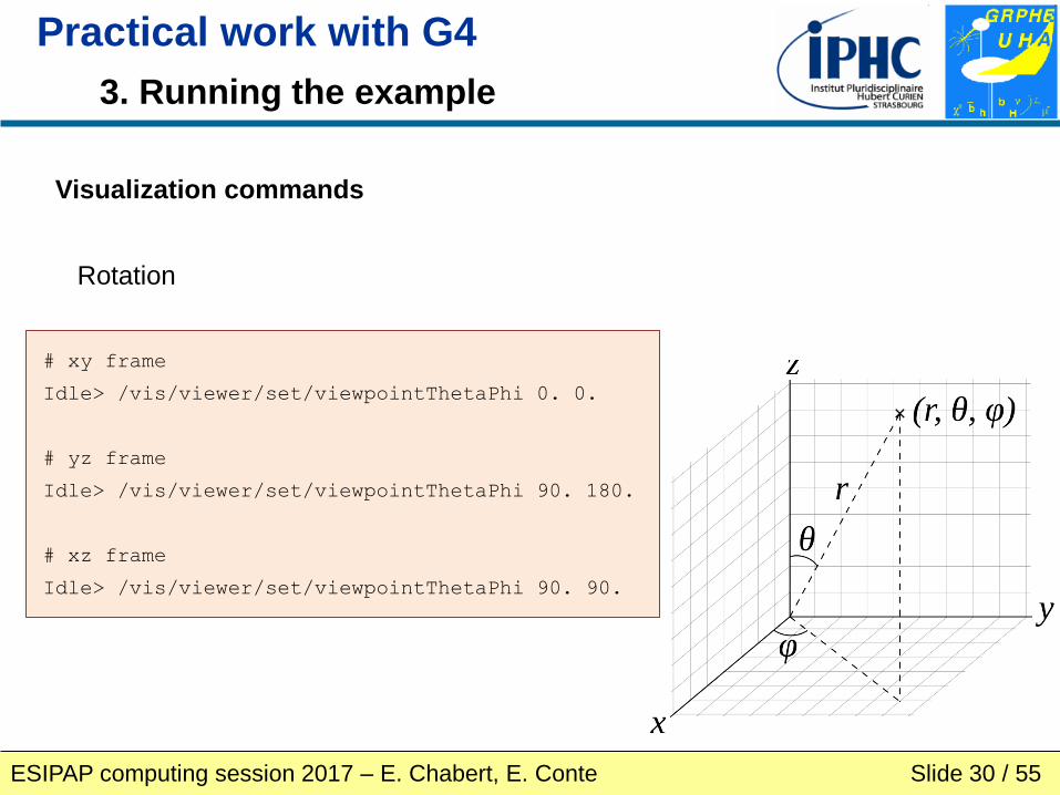
Rotation

# xy frame

Idle> /vis/viewer/set/viewpointThetaPhi 0. 0.

# yz frame


# xz frame






Rotation

# xy frame

Idle> vis/viewer/set/viewpointVector 1 0 0

# yz frame


# xz frame





Magnetic field

A global and uniform magnetic field can be activated in this example.

Changing the magnetic field consists in setting the vector components.

For instance:

Idle> /globalField/setValue 0.2 0 0 tesla




Particle Gun

• The ParticleGun tools allows you to generate a single particle with a given

momentum which can interact with your detector. Example of commands:

Idle> /gun/particle e- # kind of particle

Idle> /gun/energy 1 GeV # energy of the incident particle

Idle> /gun/position 0 0 0 cm # coordinate point (x,y,z) of the origin

Idle> /gun/direction 0 0 1 # momentum direction (px,py,pz)

• The particle kind is specified by a label.

The list of the available labels can be displayed by the command:

Idle> /gun/list




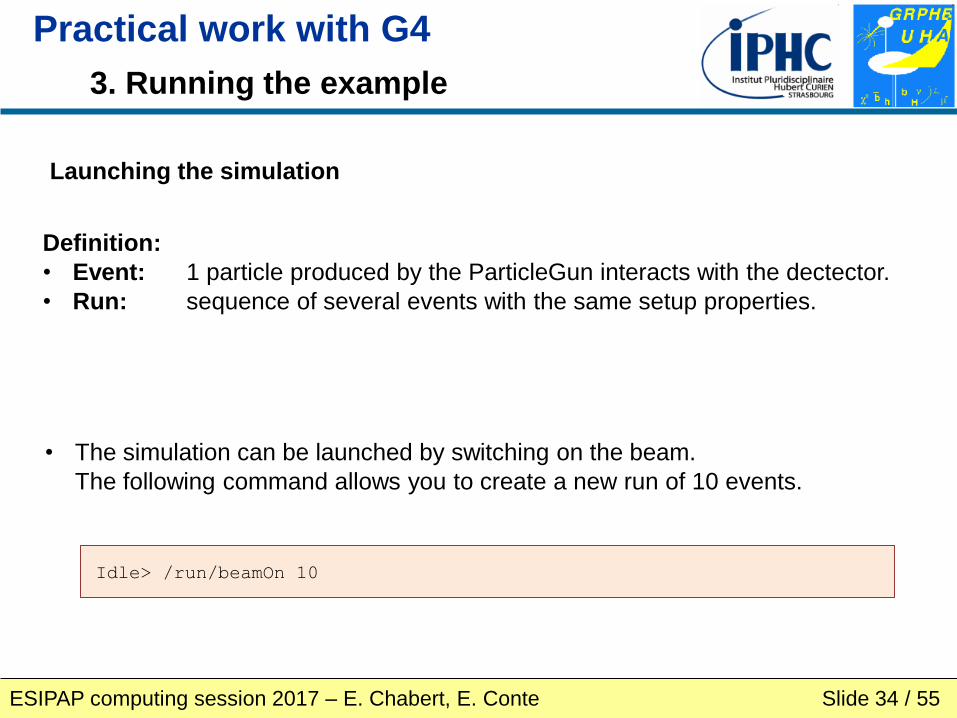
Launching the simulation

• The simulation can be launched by switching on the beam.

The following command allows you to create a new run of 10 events.

Definition:

• Event: 1 particle produced by the ParticleGun interacts with the dectector.

• Run: sequence of several events with the same setup properties.

Idle> /run/beamOn 10




Using macros

It is possible to put all the commands you type in a text file and to

load them in one time. A such text file is called a “macro” and the file

extension used for it is “.mac”.

For example: when you launch the example, a macro called

“init_vis.mac” is loaded.




Using macros

init_vis.mac

# Macro file for the initialization of example B4 in interactive session

#

# Set some default verbose

#

/control/verbose 2

/control/saveHistory

/run/verbose 2

#

# Change the default number of threads (in multi-threaded mode)

#/run/numberOfThreads 4

#

# Initialize kernel

/run/initialize

#

# Visualization setting

/control/execute vis.mac




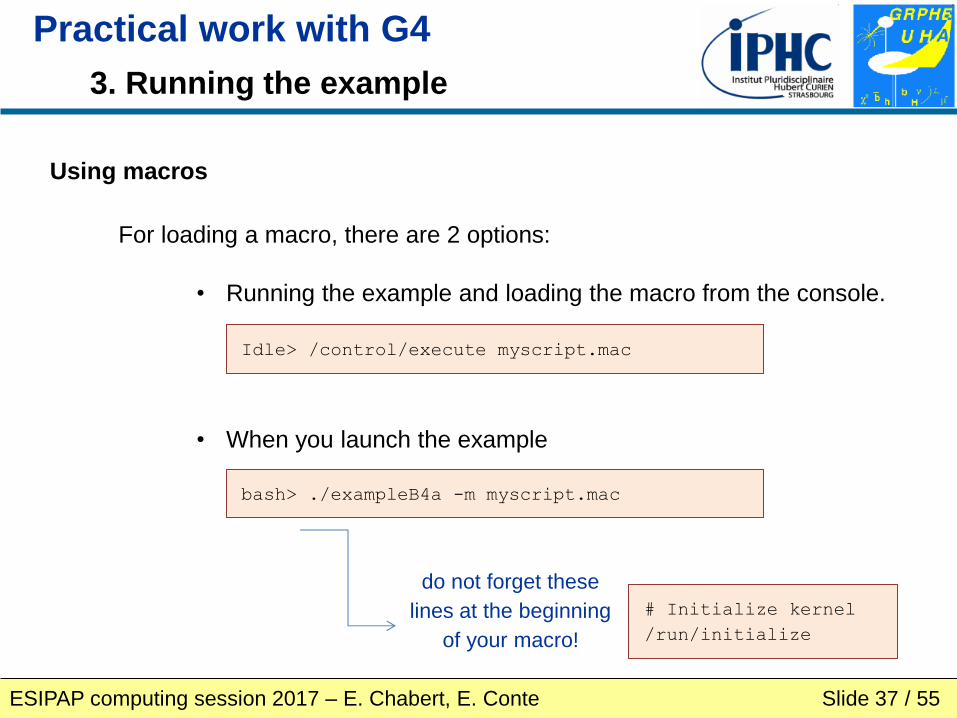
Using macros

For loading a macro, there are 2 options:

• Running the example and loading the macro from the console.

• When you launch the example

Idle> /control/execute myscript.mac

bash> ./exampleB4a -m myscript.mac

# Initialize kernel

/run/initialize

do not forget these

lines at the beginning

of your macro!


4. Studying the simulation in Example B4a


4. Studying the simulation in

Example B4a




Analyzing the simulation 1

• Before launching the simulation, it is advised to set the level of verbosity of the

program.

Idle> /run/verbose 0

Idle> /event/verbose 0

Idle> /tracking/verbose 0



• Comment what you see





Default color code:

• Track with charge = 0 green

• Track with charge = -1 red

• Track with charge = +1 blue

• Step point = yellow


• If you produce a run of several events, only the last event is showed.

You have the option to review all the last events with the command:




Idle> vis/reviewKeptEvents

• There is also a way to superimpose the events on the graphics window.

Type this command before the generation.

Idle> /vis/scene/endOfEventAction accumulate

• Graphical visualization requires time resource. There is an option to disable the

visualization for big number of events.

Idle> /vis/disable


For each event, the code of Example B4a extracts the energy deposit and the

track length in each kind of material. These values are dumped at the screen.

EAbs : mean = 44.680813750829 MeV rms = 4.480475001769 MeV

EGap : mean = 1.0744818487411 MeV rms = 1.7299239878681 MeV

LAbs : mean = 3.2189971903885 cm rms = 3.2792112794795 mm

LGap : mean = 5.716367983443 mm rms = 9.3492140235363 mm

Absorber: total energy: 40.667624006703 MeV

total track length: 3.0357196656771 cm

Gap: total energy: 848.54860464357 keV

total track length: 5.0632623359409 mm

Specifities of Example B4a : energy deposit & track length

At the end of the run, Example B4a displays the mean value and the root mean

square value of the different distributions.




Specifities of Example B4a : the ROOT file

For each event, we monitor the 4 following observables:

• Energy deposit in the absorber

• Track length in the absorber

• Energy deposit in the gap

• Track length in the gap

They are stored in a ROOT file called « B4.root ».

To dump the content of this file, you need to use ROOT.

bash> root –l B4.root

Root[1] TBrowser d




Specifities of Example B4a : the ROOT file






program.









=====================================

G4EventManager::ProcessOneEvent()

=====================================

G4PrimaryTransformer::PrimaryVertex (0(mm),0(mm),-90(mm),0(nsec))

1 primaries are passed from G4EventTransformer.

!!!!!!! Now start processing an event !!!!!!!

Track (trackID 1, parentID 0) is processed with stopping code 2






. . .



• For each event, we have a list of the tracks produced.

Stopping code? See the file

G4TrackStatus.hh






program.









********************************************************************************************

* G4Track Information: Particle = e-, Track ID = 1, Parent ID = 0

********************************************************************************************

Step# X(mm) Y(mm) Z(mm) KinE(MeV) dE(MeV) StepLeng TrackLeng NextVolume ProcName

0 0 0 -90 50 0 0 0 World initStep

1 0 -0.134 -75 50 5.25e-25 15 15 Abso Transportation

2 0.025 -0.139 -74.6 2.46 0.646 0.45 15.5 Abso eBrem

3 0.632 -0.138 -74.2 0.695 1.64 1.44 16.9 Abso eBrem

4 0.631 -0.105 -74.2 0 0.695 0.468 17.4 Abso eIoni




• More info on each track produced.




Exercise 1

• Compare the results of the

simulation for different incident

particle:

• Photon

• Electron

• Electronic neutrino

• Proton

To do




Exercise 2

• Inject the incident particle from

behind the detector.

To do



e-


5. Analyzing & editing the main program


5. Analyzing & editing

the main program


6. Analyzing & editing the detector description



the detector description


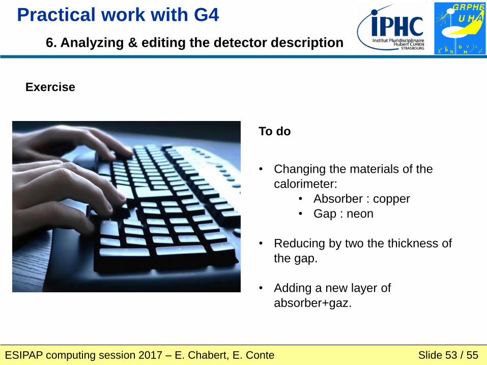
Exercise

• Changing the materials of the

calorimeter:

• Absorber : copper

• Gap : neon

• Reducing by two the thickness of

the gap.

• Adding a new layer of

absorber+gaz.

To do

6. Analyzing & editing the detector description



7. Analyzing & editing the action description



the action description


Exercise

• Display at the end of each event

the energy ratio measured by the

absorber.

• Getting energy in each layer of

absorber and saving these data

in the ROOT file

To do

7. Analyzing & editing the action description


practical work with g4 - lip

Documents