practical modellingof the incremental risk charge in the
TRANSCRIPT

© 2009 R2 Financial Technologies
Practical Modelling Of the
Incremental Risk Charge In
The Trading Book
Dan RosenR2 Financial Technologies
Fields Institute [email protected]
RiskLab Conference Madrid, September 17, 2009
Joint with David Saunders
© 2009 R2 Financial Technologies 2
Preface…
The current events have highlighted the need for transparency
� Consistent valuation and risk methodologies across asset classes
� Detailed modelling of instruments and collateral
� Counterparty credit risk
� Concentration risk and
risk contributions
� Model risk
� Stress testing
� Explicit modeling of the
interaction of market, credit,
and liquidity risk

© 2009 R2 Financial Technologies 3
Summary – IRC
� Revisions to the Basel II market risk framework, finalized in July 2009
� Require that banks develop a methodology for calculating a new
incremental risk charge (IRC)
� IRC: captures credit default and migration risks that are incremental
to the risks captured by market VaR
� Trading book positions on unsecuritised credit products
� Constant level of risk over the one-year capital horizon
� Liquidity horizon – positions whose credit characteristics have
improved or deteriorated are replaced so that credit characteristics are
equivalent to those at the start of the liquidity horizon
© 2009 R2 Financial Technologies 4
Summary – This Talk
1. Discuss the basic principles behind the IRC requirements
2. Present a robust methodology to compute IRC
� Discuss various modelling choices, which arise in practical implementations
� IRC methodology models the constant level of risk principle by combining
� Repeated application of single-step credit portfolio models
� Advanced convolution methods to model the constant risk principle
� Advantages:
� Transparent modelling of constant risk principle
� In contrast to a brute-force dynamic, multi-step Monte Carlo
� Does not need heavy parameterization or operational assumptions
� Easy to implement – leverages existing credit portfolio tools used by banks
� Comprehensive stress testing – understand credit risk components, risk contributions, diversification, capital benefits from long-short positions
3. Present practical examples
© 2009 R2 Financial Technologies 5
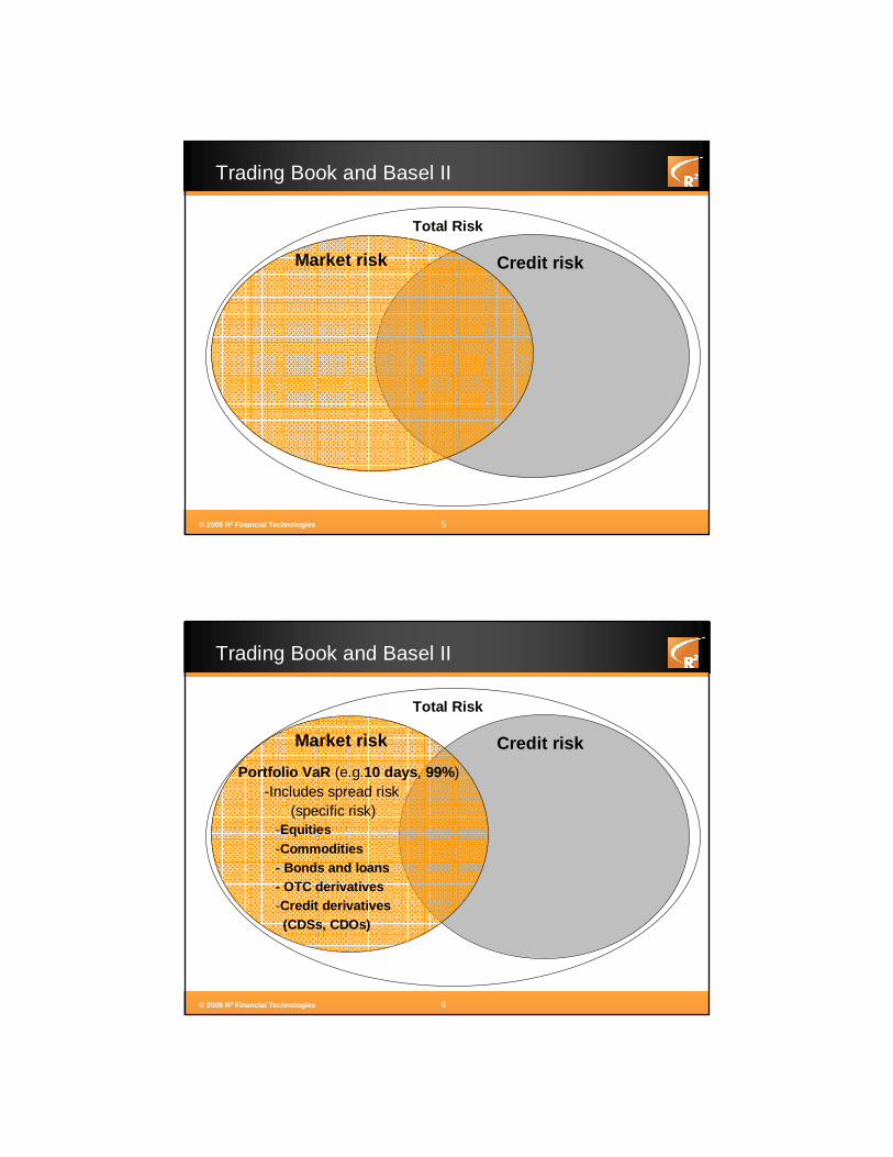
Trading Book and Basel II
Total Risk
Market risk Credit risk
© 2009 R2 Financial Technologies 6
Trading Book and Basel II
Total Risk
Market risk Credit risk
-Equities-Commodities- Bonds and loans- OTC derivatives-Credit derivatives (CDSs, CDOs)
Portfolio VaR (e.g.10 days , 99%) -Includes spread risk
(specific risk)

© 2009 R2 Financial Technologies 7
Trading Book and Basel II
Total Risk
Market risk Credit risk
Portfolio VaR (e.g.10 days , 99%) -Includes spread risk
(specific risk)
Stressed VaR (10 days , 99%) -Historical data from period of significant financial stress(e.g. 2007-2008).
© 2009 R2 Financial Technologies 8
Trading Book and Basel II
Total Risk
Credit risk1. Counterparty credit risk
– derivatives including credit
– collateral, guarantees, mitigation
2. Issuer/borrower risk – bonds, loans, CDSs
3. Structured Credit – issuer/borrower + CP
Market risk

© 2009 R2 Financial Technologies 9
Trading Book and Basel II
Total Risk
Market risk Credit risk
CreditVaR (Basel II - 1y, 99.9%)
• Counterparty credit risk (CCR)
- OTC derivatives, CDSs (CDOs)
• Incremental risk charge (IRC)- Default, migration
- Bonds, loans, CDSs
• Securitization(and correlation trading)
© 2009 R2 Financial Technologies 10
Revisions to the Basel II Market Risk and IRC
Market Risk (Internal Models Approach):
� General Market Risk Charge (10 days, 99% VaR):� Stressed Market Risk Charge (10 days, 99%)
� Calibrated to historical data from a period of significant financial stress (e.g. 2007-2008)
� Specific Risk Charge� Incremental Risk Charge (IRC) – default and migration risk
� Measured at a 99.9% confidence level, with a one-year time horizon, under the constant level of risk assumption
� Structured credit� Correlation trading: standardized and comprehensive treatment
� Securitizations – outside of IRB
� Conservative, standardized charge
© 2009 R2 Financial Technologies 11
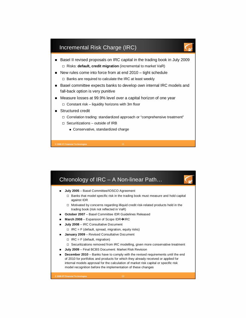
Incremental Risk Charge (IRC)
� Basel II revised proposals on IRC capital in the trading book in July 2009
� Risks: default, credit migration (incremental to market VaR)
� New rules come into force from at end 2010 – tight schedule
� Banks are required to calculate the IRC at least weekly
� Basel committee expects banks to develop own internal IRC models and fall-back option is very punitive
� Measure losses at 99.9% level over a capital horizon of one year
� Constant risk – liquidity horizons with 3m floor
� Structured credit
� Correlation trading: standardized approach or “comprehensive treatment”
� Securitizations – outside of IRB
� Conservative, standardized charge
© 2009 R2 Financial Technologies 12
Chronology of IRC – A Non-linear Path…
� July 2005 – Basel Committee/IOSCO Agreement
� Banks that model specific risk in the trading book must measure and hold capital against IDR
� Motivated by concerns regarding illiquid credit risk-related products held in the trading book (risk not reflected in VaR)
� October 2007 – Basel Committee IDR Guidelines Released
� March 2008 – Expansion of Scope IDR�IRC
� July 2008 – IRC Consultative Document
� IRC = F (default, spread, migration, equity risks)
� January 2009 – Revised Consultative Document
� IRC = F (default, migration)
� Securitizations removed from IRC modelling, given more conservative treatment
� July 2009 – Final BCBS Document: Market Risk Revision
� December 2010 – Banks have to comply with the revised requirements until the end of 2010 for portfolios and products for which they already received or applied for internal models approval for the calculation of market risk capital or specific risk model recognition before the implementation of these changes

© 2009 R2 Financial Technologies 13
� Basel guidance on setting liquidity horizons
� Time required to sell position or hedge all material risks in a stressed market
� Sufficiently long so that selling/hedging does not materially affect prices
� Floor of three months
� Non-investment expected to have longer horizons than investment grade
� Concentrated positions expected to have longer liquidity horizons
Constant Risk and Liquidity Horizons
� Capital horizon : time over which credit events are measured (1-year)
� Liquidity horizon : frequency at which the portfolio (or transaction) is
rebalanced to a target level of risk (e.g. 3m, 6m, 1y)
1y
Liquid
illiquid
Capital Horizon
Liquidity Horizons
© 2009 R2 Financial Technologies 14
Constant Risk and Liquidity Horizon
� Constant risk assumption – liquidity shorter than capital horizon
� Estimation of liquidity horizon PDs – ratings data, KMV/market, implied from transition matrices (roots)
Example of PD effect
T0 T1 T2
IG
NIG
D
IG NIG D
IG 0.2 0.7 0.1
NIG 0.1 0.1 0.8
D 0 0 1
� PD (Constant Position, 2 periods) = 0.1×1 + 0.7×0.8 + 0.2×0.1 = 0.68
� PD (Constant Risk, 2 periods) = 0.1×1 + 0.9×0.1 = 1 – (1-.01)^2 = 0.19
© 2009 R2 Financial Technologies 15
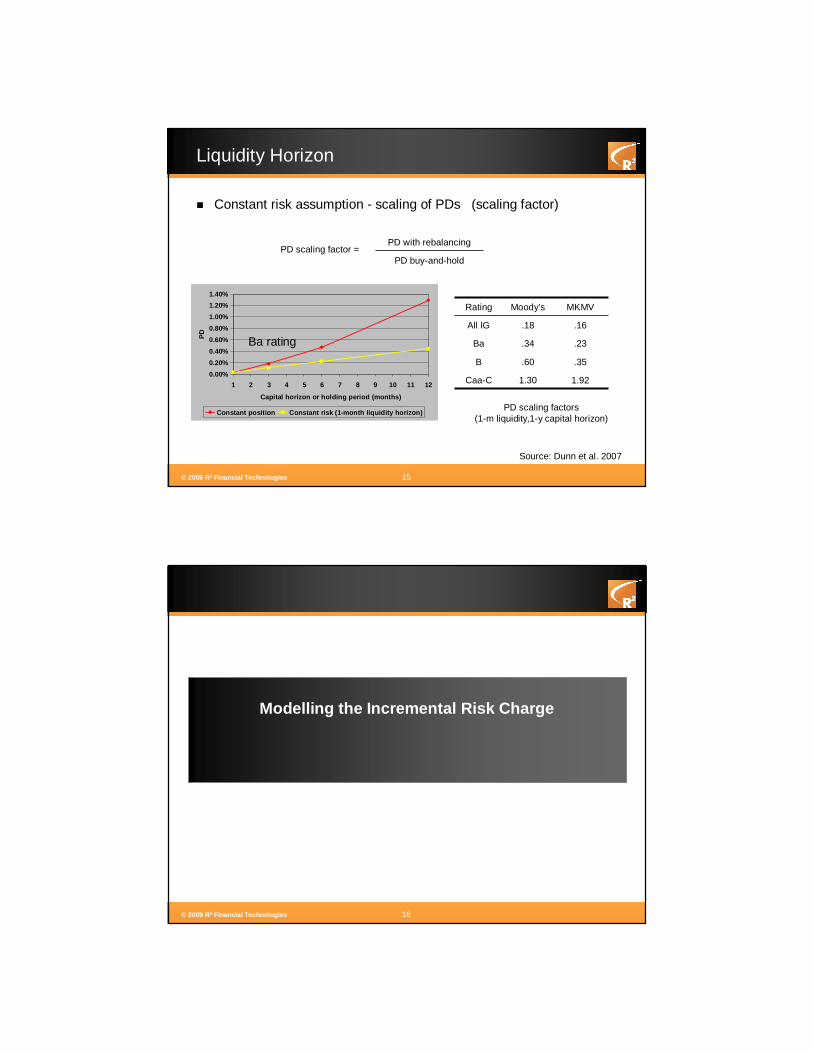
Liquidity Horizon
� Constant risk assumption - scaling of PDs (scaling factor)
0.00%
0.20%
0.40%
0.60%
0.80%
1.00%
1.20%
1.40%
1 2 3 4 5 6 7 8 9 10 11 12
Capital horizon or holding period (months)
PD
Constant position Constant risk (1-month liquidity horizon)
Ba rating
Source: Dunn et al. 2007
Rating Moody’s MKMV
All IG .18 .16
Ba .34 .23
B .60 .35
Caa-C 1.30 1.92
PD scaling factors (1-m liquidity,1-y capital horizon)
PD scaling factor =PD with rebalancing
PD buy-and-hold
© 2009 R2 Financial Technologies 16
Modelling the Incremental Risk Charge
© 2009 R2 Financial Technologies 17
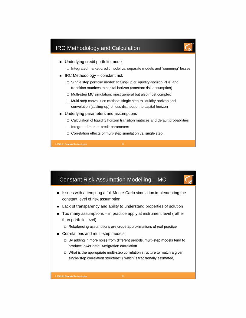
IRC Methodology and Calculation
� Underlying credit portfolio model
� Integrated market-credit model vs. separate models and “summing” losses
� IRC Methodology – constant risk
� Single step portfolio model: scaling-up of liquidity-horizon PDs, and
transition matrices to capital horizon (constant risk assumption)
� Multi-step MC simulation: most general but also most complex
� Multi-step convolution method: single step to liquidity horizon and
convolution (scaling-up) of loss distribution to capital horizon
� Underlying parameters and assumptions
� Calculation of liquidity horizon transition matrices and default probabilities
� Integrated market-credit parameters
� Correlation effects of multi-step simulation vs. single step
© 2009 R2 Financial Technologies 18
Constant Risk Assumption Modelling – MC
� Issues with attempting a full Monte-Carlo simulation implementing the
constant level of risk assumption
� Lack of transparency and ability to understand properties of solution
� Too many assumptions – in practice apply at instrument level (rather
than portfolio level)
� Rebalancing assumptions are crude approximations of real practice
� Correlations and multi-step models
� By adding in more noise from different periods, multi-step models tend to
produce lower default/migration correlation
� What is the appropriate multi-step correlation structure to match a given
single-step correlation structure? ( which is traditionally estimated)

© 2009 R2 Financial Technologies 19
Constant Risk Modelling Objectives
� Transparent
� Risk-sensitive
� Simple
� Small number of meaningful parameters
� Constant risk principle imposed at the portfolio level – rather than at
each position independently
� Easy to parameterize and consistent with single-step credit portfolio
parameter estimates
� Reuse existing infrastructure (single step modelling)
� Meaningful intuition for stress testing and assessing model risk
� Benchmarking
© 2009 R2 Financial Technologies 20
Proposed IRC Methodology
1. Basic credit model building block : single-step credit portfolio model
� Loses and EC(t) for a given capital horizon t
� Loss decomposition: default vs. MtM, systematic vs. idiosyncratic
2. Capital horizon curves : multiple single-step credit portfolio losses� t= 1m, 3m, 6m, 1y
� Calculation for portfolio and sub-portfolios
3. Constant risk capital curves (liquidity horizon) – scaling � Convolution (homogeneous liquidity): EC(t) � EC(T=1y)
� Alternatives: simple time-scaling: e.g. sqrt(t), “ad-hoc” factor
4. Aggregation and inhomogeneous portfolios� Definition of “liquidity sub-portfolios”
� Inhomogeneous liquidity (or non-standard liquidity horizon)
� Multi-step convolution and copulas for inhomgeneous horizons
� Interpolation: weighted-averages

© 2009 R2 Financial Technologies 21
Exposures
DefaultMigration
Recovery
t
0 t
1. Portfolio Credit Risk Model: Components
© 2009 R2 Financial Technologies 22
General Credit Portfolio Model
1. Scenarios: � market factors � credit drivers
2. Conditional def./mig. probabilities
. . . . . AA
BBB
CCC
3. Conditional instrument prices & CP exposures. . . . . . .
Default
. . . . . . . . . . . . . . . . . . . . . . . . . . . . . . . . . . . .
4. Conditional portfolio losses
+
+
______5. Unconditional
Portfolio loss distribution

© 2009 R2 Financial Technologies 23
IRC Methodology
1. Single-step credit portfolio model
� Loses and EC(t) for a given capital horizon t
� Loss decomposition: default vs. MtM, systematic vs. idiosyncratic
2. Capital horizon curve – multiple single-step credit portfolio losses� t= 1m, 3m, 6m, 1y
� Calculation for portfolio and sub-portfolios
� Repeated simulation applying the single step portfo lio model fordifferent liquidity horizons
� Scaling of default probabilities and correlations.
© 2009 R2 Financial Technologies 24
2. Capital Horizon Curves
Capital horizon curve
� EC(t) = f (t=capital horizon)
t
EC
1m 3m 6m 1y

© 2009 R2 Financial Technologies 25
IRC Methodology
1. Single-step credit portfolio model
� Loses and EC(t) for a given capital horizon t
� Loss decomposition: default vs. MtM, systematic vs. idiosyncratic
2. Capital horizon curve – multiple single-step credit portfolio losses� t= 1m, 3m, 6m, 1y
� Calculation for portfolio and sub-portfolios
3. Constant risk capital (liquidity horizon) curve – sc aling
� EC(t) ���� EC(T=1y)
� Convolution (consecutive horizon periods are indepe ndent)
� Alternatives: simple time-scaling: e.g. sqrt(t) , “ad-hoc” factor
� Calculate economic capital under the constant level of risk assumption (through simplified scaling).
� Assume entire portfolio has the same liquidity hori zon.
© 2009 R2 Financial Technologies 26
IRC – Capital and Liquidity Horizon
3m
1y
** * =
Example:Convolution method

© 2009 R2 Financial Technologies 27
Constant Risk Curves (Liquidity Horizon)
Capital horizon curve
� EC(t) = f (t=capital horizon)
Constant risk curve� EC (T=1y) = f (t=liquidity horizon)
t
EC
1m 3m 6m 1y
This is normally done assuming all trades in the portfolio have the same liquidity horizon (homogeneous case)
© 2009 R2 Financial Technologies 28
IRC Methodology
1. Single-step credit portfolio model
� Loses and EC(t) for a given capital horizon t
� Loss decomposition: default vs. MtM, systematic vs. idiosyncratic
2. Capital horizon curve – multiple single-step credit portfolio losses� t= 1m, 3m, 6m, 1y
� Calculation for portfolio and sub-portfolios
3. Constant risk capital (liquidity horizon) curve – scaling � Convolution (homogeneous liquidity): EC(t) � EC(T=1y)
� Alternatives: simple time-scaling: e.g. sqrt(t), “ad-hoc” factor
4. Aggregation and inhomogeneous portfolios� Definition of “ liquidity sub-portfolios ”
� Inhomogeneous liquidity (or non-standard liquidity horizon)
� Multi-step inhomgeneous convolution and copulas
� Interpolation: weighted-averages

© 2009 R2 Financial Technologies 29
Inhomogeneous Portfolios and Interpolation
� Interpolation based on upper and lower bounds (C. Finger, 2009).
� Example lower bounds: IRC calculated assuming homogeneous liquidity horizon of 3 months and 1 year.
� where λ is determined by the liquidity horizons of instruments in the portfolio.
� Select the IRC corresponding to the point on the liquidity horizon curve with the ‘portfolio average liquidity horizon’:
� Possible choices for weights include % exposures, % expected losses, capital contributions,…
IRC = λ ⋅ IRCL + (1− λ) ⋅ IRCU
LH = wnLHn , wn =1n
∑n
∑
© 2009 R2 Financial Technologies 30
Multi-step Convolution with Copulas
� Final step can be computed using a multi-step convolution technique and copula codependence of sub-portfolio losses� Dynamic (multi-step) single-factor
� Captures effectively constant risk within inhomogeneous portfolios (liquidity horizons)
� Example:� Portfolio P = P1 + P2 + P4 – sub-portfolios have liquidity 3m, 6m, 1y respectively
� Portfolio Losses L = L1 + L2 + L4
� Single factor credit factor Z
� Individual losses at their liquidity horizon computed using single-step credit portfolio model: L1(t1), L2(t2), L4(t4)
� Single factor copula model for L as follows:
� Correlation estimated directly from single-step simulation
( )( )( )( )( )212
122
2221
2
, ZZZXCorrr
tLFX
+==Φ= − ( )( )( )
( )∑ =
−
==
Φ=4
121
33
4331
3
,i iZZXCorrr
tLFX
Z(t1) Z(t2) Z(t3) Z(t4)
( )( )( )( )111
1111
1
, ZZXCorrr
tLFX
==Φ= −
© 2009 R2 Financial Technologies 31
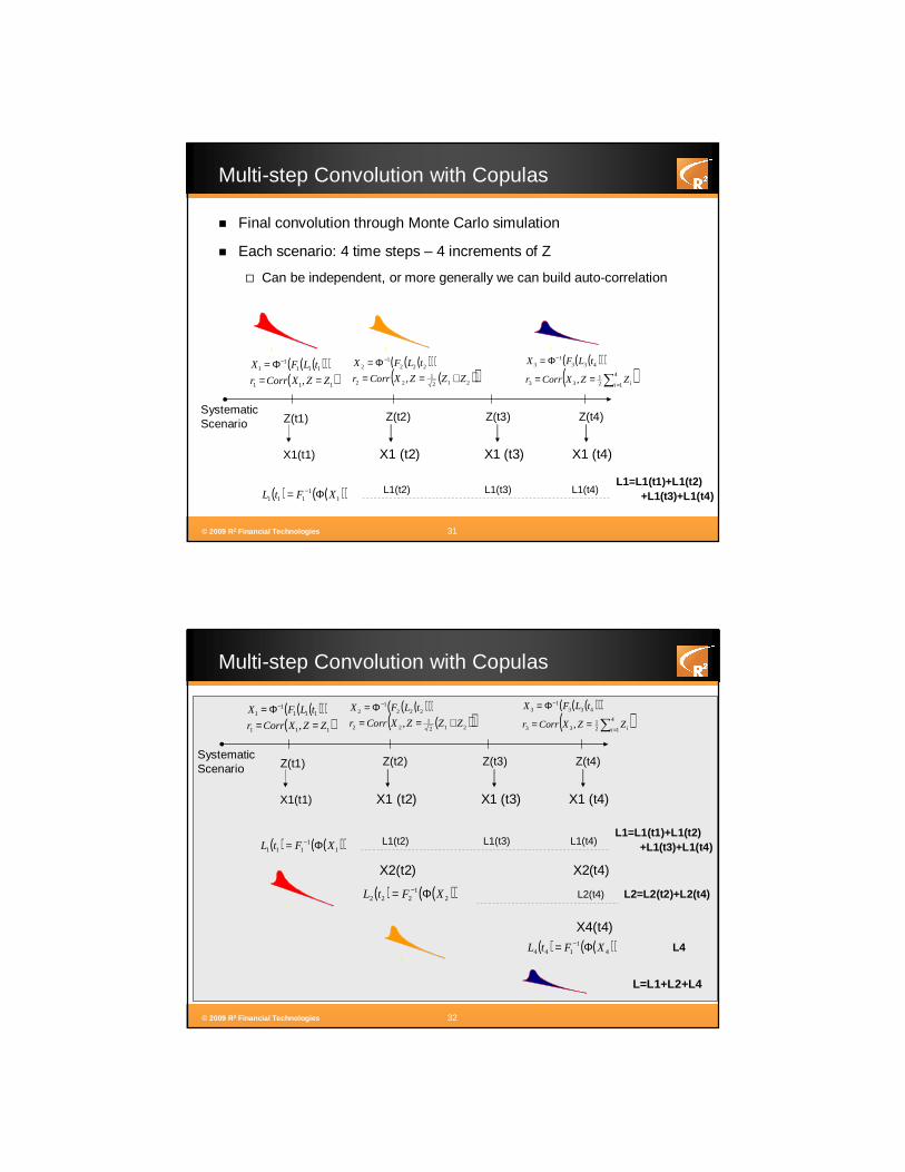
Multi-step Convolution with Copulas
� Final convolution through Monte Carlo simulation
� Each scenario: 4 time steps – 4 increments of Z
� Can be independent, or more generally we can build auto-correlation
( )( )( )( )( )212
122
2221
2
, ZZZXCorrr
tLFX
+==Φ= − ( )( )( )
( )∑ =
−
==
Φ=4
121
33
4331
3
,i iZZXCorrr
tLFX
SystematicScenario Z(t1) Z(t2) Z(t3) Z(t4)
( )( )( )( )111
1111
1
, ZZXCorrr
tLFX
==Φ= −
X1(t1) X1 (t2) X1 (t3) X1 (t4)
( ) ( )( )11
111 XFtL Φ= −L1=L1(t1)+L1(t2)
+L1(t3)+L1(t4)L1(t2) L1(t3) L1(t4)
© 2009 R2 Financial Technologies 32
Multi-step Convolution with Copulas
( )( )( )( )( )212
122
2221
2
, ZZZXCorrr
tLFX
+==Φ= − ( )( )( )
( )∑ =
−
==
Φ=4
121
33
4331
3
,i iZZXCorrr
tLFX
( ) ( )( )21
222 XFtL Φ= −
SystematicScenario Z(t1) Z(t2) Z(t3) Z(t4)
( )( )( )( )111
1111
1
, ZZXCorrr
tLFX
==Φ= −
X1(t1) X1 (t2) X1 (t3) X1 (t4)
( ) ( )( )11
111 XFtL Φ= −L1=L1(t1)+L1(t2)
+L1(t3)+L1(t4)
( ) ( )( )41
144 XFtL Φ= −
L2=L2(t2)+L2(t4)
X4(t4)
L4
L=L1+L2+L4
L1(t2) L1(t3) L1(t4)
X2(t2) X2(t4)
L2(t4)

© 2009 R2 Financial Technologies 33
Examples
© 2009 R2 Financial Technologies 34
Example - Portfolio
� Portfolio: CDS and bonds, ~3,500 positions
� 425 Issuers (170 overall long issuers)
� Slightly negative cash equivalent value (CEV)
CEV By Posit ion
0% 10% 20% 30% 40% 50% 60%Percent of Portfolio
Long
Short
Concentration by Rating: Total CEV
AAA, 0.2%
A, 128.5%
BB, -135.4%
B, -75.0%
, AA, 3.0%
CCC, -8.5%
© R2 Financial Technologies Inc.
Effective Issuers
0
50
100
150
200
1 26 51 76 101 126 151 176 201 226 251 276 301 326 351 376 401 426Issuers
No
Eff
Issu
ers
Issuer Size
0
20
40
60
80
100
2.E+0
7
3.E+06
4.E+0
5
6.E+04
0.E+0
0
-6.E
+04
-4.E
+05
-3.E
+06
-2.E
+07
CEV
Fre
quen
cy
CEV

© 2009 R2 Financial Technologies 35
Transition Matrix
AAA AA A BBB BB B CCC D
AAA 0.92316 0.06735 0.00717 0.00083 0.00125 0.00011 0.00002 0.00011
AA 0.00595 0.91217 0.07055 0.00825 0.00113 0.00144 0.00029 0.00023
A 0.00064 0.01796 0.91791 0.05406 0.00593 0.00223 0.00034 0.00092
BBB 0.00022 0.00195 0.03810 0.90378 0.04208 0.00919 0.00141 0.00328
BB 0.00040 0.00080 0.00394 0.05178 0.84643 0.07464 0.00767 0.01435
B 0.00002 0.00074 0.00225 0.00457 0.05127 0.84682 0.03566 0.05868
CCC 0.00000 0.00008 0.00327 0.00514 0.01282 0.08201 0.64225 0.25443
D 0.00000 0.00000 0.00000 0.00000 0.00000 0.00000 0.00000 1.00000
AAA AA A BBB BB B CCC D
AAA 0.98017 0.01795 0.00139 0.00013 0.00033 0.00001 0.00000 0.00003
AA 0.00158 0.97709 0.01883 0.00179 0.00023 0.00036 0.00008 0.00003
A 0.00016 0.00479 0.97845 0.01447 0.00136 0.00051 0.00008 0.00019
BBB 0.00005 0.00044 0.01019 0.97454 0.01157 0.00214 0.00035 0.00071
BB 0.00011 0.00019 0.00083 0.01427 0.95842 0.02105 0.00201 0.00311
B 0.00000 0.00019 0.00056 0.00091 0.01447 0.95838 0.01114 0.01435
CCC 0.00000 0.00001 0.00094 0.00143 0.00338 0.02560 0.89470 0.07395
D 0.00000 0.00000 0.00000 0.00000 0.00000 0.00000 0.00000 1.00000
1 year
3 months
© 2009 R2 Financial Technologies 36
Example – Conditional Loss Matrices
Loss at 1Y Horizon*
Initial State Issuers AAA AA A BBB BB B CCC DLong AAA 0 - - - - - - - -
AA 12 0.0 0.0 -0.1 0.4 5.1 6.4 23.6 39.9A 21 -0.2 -0.1 0.0 1.0 6.0 8.0 25.6 40.5
BBB 53 -2.5 -2.2 -1.5 0.0 1.5 10.4 32.8 41.7BB 52 -8.4 -8.0 -6.6 -3.7 0.0 10.8 35.4 39.2
B 28 -33.7 -32.8 -29.8 -25.2 -23.7 0.0 37.4 30.0CCC 9 -93.7 -92.4 -88.0 -81.4 -76.1 -48.5 0.0 -3.5
Short AAA 2 0.0 0.0 0.0 0.0 -1.0 -5.1 -13.2 -40.3AA 14 0.2 0.0 -0.9 -2.7 -4.1 -8.8 -14.1 -33.5
A 64 1.0 0.8 0.0 -1.4 -2.5 -7.9 -14.5 -32.0BBB 122 3.1 2.7 1.7 0.0 -0.2 -7.9 -15.6 -33.0
BB 39 1.9 1.5 1.1 0.3 0.0 -7.0 -14.2 -32.3B 7 1.4 1.4 1.3 1.3 0.8 0.0 -0.9 -20.4
CCC 4 0.0 0.0 0.0 0.0 0.0 0.0 0.0 -14.7Overall AAA 2 0.0 0.0 0.0 0.0 -1.0 -5.1 -13.2 -40.3
AA 26 7.6 0.0 -30.9 -67.0 25.7 -75.8 254.5 148.6A 85 2.0 1.6 0.0 -1.8 1.5 -7.7 -1.6 -22.1
BBB 175 4.3 3.6 1.9 0.0 2.1 -3.4 15.2 -17.2BB 91 -13.0 -12.4 -10.5 -6.0 0.0 13.4 50.2 44.0
B 35 -37.5 -36.5 -33.1 -28.0 -26.4 0.0 41.7 31.1CCC 13 -244.4 -241.0 -229.4 -212.3 -198.5 -126.5 0.0 -32.8
* % of CEV (t0) © R2 Financial Technologies Inc.
Exposure Summary
Credit Scenario

© 2009 R2 Financial Technologies 37
Example – Constant Portfolio Capital
CEV(net) CEV(gross) EL Sigma CVaR 99.9% VaR 90% VaR 95% VaR 99% VaR 99.5% VaR 99.9%Total -1.04 100.00 0.02 0.08 0.31 0.12 0.16 0.25 0.29 0.39
Systematic 0.02 0.06 0.22 0.09 0.12 0.18 0.21 0.26Idiosyncratic 23.5% 30.3% 18.4% 21.6% 27.1% 29.0% 33.3%
Stand-Alone Long 48.10 48.10 0.19 0.35 1.87 0.62 0.85 1.44 1.73 2.42Systematic 0.19 0.33 1.77 0.59 0.81 1.37 1.64 2.30
Idiosyncratic 6.0% 4.9% 4.2% 4.8% 4.9% 4.9% 5.1%
Portfolio A -1.37 33.22 0.00 0.01 0.05 0.00 0.01 0.03 0.04 0.06Systematic 0.00 0.00 0.00 0.00 0.00 0.00 0.00 0.01
Idiosyncratic 71.2% 90.8% 73.5% 73.0% 88.4% 91.3% 90.6%
Portfolio B 0.33 66.78 0.02 0.08 0.32 0.12 0.16 0.26 0.30 0.40Systematic 0.02 0.06 0.23 0.10 0.13 0.20 0.22 0.28
Idiosyncratic 21.5% 26.6% 16.7% 19.4% 24.0% 25.5% 29.4%
© R2 Financial Technologies Inc.
Default and Migration Risk @ 1 Year Horizon
Default and Migration Losses*
Total Loss Histogram
0
10
20
30
40
50
60
70
80
BINS
-6167
23
-3138
6.2
-159
7.31
-81.2
903
-4.1370
2
-0.2105
41
0.68506
7
14.8904
323.652
7034.7
8
15290
5
3.32E+06
Loss
Fre
quen
cy (
Tho
usan
ds)
Systematic Default VaR by Percentile
-40
-30
-20
-10
0
10
20
30
40
0 0.2 0.4 0.6 0.8 1
Quantile
VaR
($m
il)
Long OnlyShort OnlyOverall Portfolio
Total Loss Histogram
0
10
20
30
40
50
60
70
80
-8.E
+06
-4.E
+05
-2.E
+04
-1.E
+03
-6.E
+01
-3.E
+00
-1.E
-01
1.E+00
2.E+01
5.E+0
2
1.E+04
2.E+0
5
5.E+06
Loss
Fre
quen
cy (
Tho
usan
ds)
Systematic Migration VaR by Percentile
-40
-30
-20
-10
0
10
20
30
40
0 0.2 0.4 0.6 0.8 1
Quantile
VaR
($m
il)
Long OnlyShort OnlyOverall Portfolio
Total Loss Histogram
0
50
100
150
200
250
300
350
400
-1.E
+07
-5.E
+05
-2.E
+04
-1.E
+03
-6.E
+01
-3.E
+00
-1.E
-01
1.E+00
2.E+01
4.E+0
2
8.E+03
2.E+0
5
3.E+06
Loss
Fre
quen
cy (
Tho
usan
ds)
Systematic Default VaR by Percentile
-40
-30
-20
-10
0
10
20
30
40
0 0.2 0.4 0.6 0.8 1
Quantile
VaR
($m
il)
Long OnlyShort OnlyOverall Portfolio
Total Loss Histogram
0
10
20
30
40
50
60
70
80
90
100
-1.E
+07
-5.E
+05
-3.E
+04
-1.E
+03
-6.E
+01
-3.E
+00
-1.E
-01
1.E+00
3.E+01
6.E+0
2
1.E+04
3.E+05
8.E+06
Loss
Fre
quen
cy (
Tho
usan
ds)
Systematic Losses & Systematic Factor
-80
-60
-40
-20
0
20
40
60
80
100
0 0.2 0.4 0.6 0.8 1
CDF(Z)
Loss
es (
mill
ion)
Long OnlyShort OnlyOverall Portfolio
Total & Systematic Losses
0
0
0
0
0
0
0
0
0
0
90%Confidence Interval
VaR
(mill
ion)
Total Systematic
© 2009 R2 Financial Technologies 38
Example – Capital Horizon and Constant Risk Curves
Total Defaullt and Migration: VaR 99.9%Overall Portfolio
-
0.05
0.10
0.15
0.20
0.25
0.30
0.35
0.40
0.45
0.25 0.5 1
Capital HorizonCurve
Constant RiskCurve (Sqrt-roo t)
Constant RiskCurve
Systematic default and Migration: VaR 99.9%Stand-Alone Long
-
0.50
1.00
1.50
2.00
2.50
0.25 0.5 1
Capital HorizonCurve
Constant RiskCurve (Sqrt-roo t)
Constant RiskCurve
Systematic Default and Migration: VaR 99.9%Portfolio A
-
0.00
0.00
0.00
0.00
0.01
0.01
0.25 0.5 1
(in m
illion)
Capital HorizonCurve
Constant R iskCurve (Sqrt-root)
Constant R iskCurve
Systematic default and Migration: VaR 99.9%Portfolio B
-
0.05
0.10
0.15
0.20
0.25
0.30
0.25 0.5 1
(in m
illion
)
Capital Ho rizo nCurve
Constant RiskCurve (Sqrt-ro ot)
Constant RiskCurve
Multi-step
convolution:
Capital = 0.33

© 2009 R2 Financial Technologies 39
Example 2 – Credit Portfolio Modelling (long-short)
© 2009 R2 Financial Technologies 40
Multi-Factor Credit Losses

© 2009 R2 Financial Technologies 41
Credit Models Comparison
© 2009 R2 Financial Technologies 42
Loss Decomposition and Diversification

© 2009 R2 Financial Technologies 43
Capital Stress Tests
© 2009 R2 Financial Technologies 44
Concluding Remarks

© 2009 R2 Financial Technologies 45
Summary – This Talk
� Present a robust methodology to compute IRC
� Discuss various modelling choices, which arise in practical implementations
� IRC methodology models the constant level of risk principle by combining� Repeated application of single-step credit portfolio models
� Advanced convolution methods to model the constant risk principle
� Advantages:� Transparent modelling of constant risk principle
� In contrast to a brute-force dynamic, multi-step Monte Carlo
� Does not need heavy parameterization or operational assumptions
� Easy to implement – leverages existing credit portfolio tools used by banks
� Comprehensive stress testing – understand credit risk components, risk contributions, diversification, capital benefits from long-short positions
© 2009 R2 Financial Technologies
www.R2-financial.com