practical cfd simulations on programmable graphics ...comba/papers/2005/smac-cgf.pdf · volume 0...

Volume 0(1981), Number 0 pp. 1–12

Practical CFD Simulations on Programmable GraphicsHardware using SMAC†

Carlos E. Scheidegger1, João L. D. Comba2 and Rudnei D. da Cunha3

1 Scientific Computing and Imaging Institute, School of Computing, University of Utah,50 S. Central Campus Dr., Salt Lake City, UT 84112, United States.

[email protected] Instituto de Informática, Universidade Federal do Rio Grande do Sul, Av. Bento Goncalves, 9500,

Campus do Vale, Bloco IV-Prédio 43425, Porto Alegre RS 91501-970, [email protected]

3 Instituto de Matemática, , Universidade Federal do Rio Grande do Sul, Av. Bento Goncalves, 9500,Campus do Vale, Prédio 43111, Porto Alegre RS 91509-900, Brazil.

[email protected]

AbstractThe explosive growth in integration technology and the parallel nature of rasterization-based graphics APIschanged the panorama of consumer-level graphics: today, GPUs are cheap, fast and ubiquitous. We show howto harness the computational power of GPUs and solve the incompressible Navier-Stokes fluid equations signifi-cantly faster (more than one order of magnitude in average) than on CPU solvers of comparable cost. While pastapproaches typically used Stam’s implicit solver, we use a variation of SMAC (Simplified Marker and Cell). SMACis widely used in engineering applications, where experimental reproducibility is essential. Thus, we show that theGPU is a viable and affordable processor for scientific applications. Our solver works with general rectangulardomains (possibly with obstacles), implements a variety of boundary conditions and incorporates energy trans-port through the traditional Boussinesq approximation. Finally, we discuss the implications of our solver in lightof future GPU features, and possible extensions such as three-dimensional domains and free-boundary problems.

Categories and Subject Descriptors(according to ACM CCS): I.3.3 [Computer Graphics]: Line and Curve Genera-tion

1. Introduction

Using the modern programmable graphics hardware pro-cessing power for general computation is a very active areaof research [BFGS03] [GWL∗03] [GRLM03]. Although thisis not a new idea [KI99] [LM01], only recently has thegraphics hardware used in consumer-level personal com-puters become powerful enough for scientific applications,in terms of data representation, raw performance and pro-grammability.

† Based on "Navier Stokes on Programmable Graphics Hardwareusing SMAC", by C. Scheidegger, J. Comba, and R. Cunha, whichappeared in Proceedings of SIBGRAPI/SIACG 2004 (ISBN 0-77=695-2227-0).c©2004 IEEE.

Nowadays, modern GPUs have IEEE 754 numbersthroughout the pipeline, with highly programmable vertexand fragment units. The GPUs have been described asstreamprocessors[PBMH02] [CDPS03], where streams are definedas sets of independent uniform data. This is mostly whyGPUs are so fast: since computations on pieces of the streamare independent from each other, it is possible to use multi-ple functional units to process the data efficiently, in parallel.

Obviously, some problems are not easily decomposablein independent pieces. A GPU algorithm is, in most cases,a carefully constructed sequence of graphics API calls, withtextures serving as storage for data structures, and vertex andfragment programs serving as computational engines. Often,the algorithm must be significantly changed to be amenableto GPU implementation [HMG03]. For our solver, we use

c© The Eurographics Association and Blackwell Publishing 2005. Published by BlackwellPublishing, 9600 Garsington Road, Oxford OX4 2DQ, UK and 350 Main Street, Malden,MA 02148, USA.

Carlos E. Scheidegger & João L. D. Comba & Rudnei D. Cunha / Practical CFD Simulations using SMAC

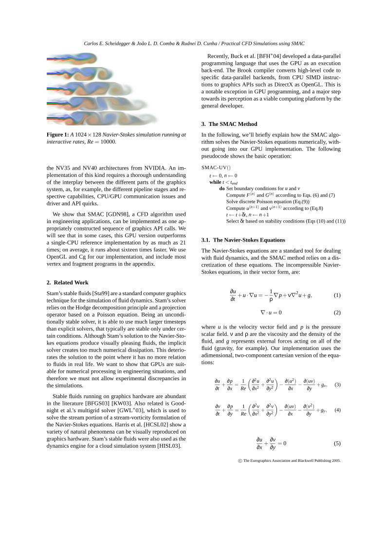
Figure 1: A 1024×128Navier-Stokes simulation running atinteractive rates, Re= 10000.

the NV35 and NV40 architectures from NVIDIA. An im-plementation of this kind requires a thorough understandingof the interplay between the different parts of the graphicssystem, as, for example, the different pipeline stages and re-spective capabilities, CPU/GPU communication issues anddriver and API quirks.

We show that SMAC [GDN98], a CFD algorithm usedin engineering applications, can be implemented as one ap-propriately constructed sequence of graphics API calls. Wewill see that in some cases, this GPU version outperformsa single-CPU reference implementation by as much as 21times; on average, it runs about sixteen times faster. We useOpenGL and Cg for our implementation, and include mostvertex and fragment programs in the appendix.

2. Related Work

Stam’s stable fluids [Sta99] are a standard computer graphicstechnique for the simulation of fluid dynamics. Stam’s solverrelies on the Hodge decomposition principle and a projectionoperator based on a Poisson equation. Being an uncondi-tionally stable solver, it is able to use much larger timestepsthan explicit solvers, that typically are stable only under cer-tain conditions. Although Stam’s solution to the Navier-Sto-kes equations produce visually pleasing fluids, the implicitsolver creates too much numerical dissipation. This deterio-rates the solution to the point where it has no more relationto fluids in real life. We want to show that GPUs are suit-able for numerical processing in engineering situations, andtherefore we must not allow experimental discrepancies inthe simulations.

Stable fluids running on graphics hardware are abundantin the literature [BFGS03] [KW03]. Also related is Good-night et al.’s multigrid solver [GWL∗03], which is used tosolve the stream portion of a stream-vorticity formulation ofthe Navier-Stokes equations. Harris et al. [HCSL02] show avariety of natural phenomena can be visually reproduced ongraphics hardware. Stam’s stable fluids were also used as thedynamics engine for a cloud simulation system [HISL03].

Recently, Buck et al. [BFH∗04] developed a data-parallelprogramming language that uses the GPU as an executionback-end. The Brook compiler converts high-level code tospecific data-parallel backends, from CPU SIMD instruc-tions to graphics APIs such as DirectX as OpenGL. This isa notable exception in GPU programming, and a major steptowards its perception as a viable computing platform by thegeneral developer.

3. The SMAC Method

In the following, we’ll briefly explain how the SMAC algo-rithm solves the Navier-Stokes equations numerically, with-out going into our GPU implementation. The followingpseudocode shows the basic operation:

SMAC-UV()

t← 0, n← 0while t < tend

do Set boundary conditions foru andvComputeF(n) andG(n) according to Eqs. (6) and (7)Solve discrete Poisson equation (Eq.(9))Computeu(n+1) andv(n+1) according to (Eq.8)t← t+δt, n← n+1Selectδt based on stability conditions (Eqs (10) and (11))

3.1. The Navier-Stokes Equations

The Navier-Stokes equations are a standard tool for dealingwith fluid dynamics, and the SMAC method relies on a dis-cretization of these equations. The incompressible Navier-Stokes equations, in their vector form, are:

∂u∂t

+u ·∇u =−1ρ∇p+ν∇2u+g, (1)

∇·u = 0 (2)

whereu is the velocity vector field andp is the pressurescalar field.ν andρ are the viscosity and the density of thefluid, andg represents external forces acting on all of thefluid (gravity, for example). Our implementation uses theadimensional, two-component cartesian version of the equa-tions:

∂u

∂t+

∂p

∂x=

1

Re

(∂2u

∂x2+

∂2u

∂y2

)−

∂(u2)∂x−

∂(uv)∂y

+gx, (3)

∂v

∂t+

∂p

∂y=

1

Re

(∂2v

∂x2+

∂2v

∂y2

)−

∂(uv)∂x−

∂(v2)∂y

+gy, (4)

∂u∂x

+∂v∂y

= 0 (5)

c© The Eurographics Association and Blackwell Publishing 2005.


Figure 2: In a staggered grid discretization, different vari-ables are sampled at different places.

whereRe is the Reynolds number, relating viscous and dy-namic forces.

3.2. Boundary Conditions and Domain Discretization

We assume a rectangular domain[0,w]× [0,h] ⊂ R2 inwhich we restrict the simulation. This means we have todeal with the appropriate boundary conditions along the bor-ders of the domain. We implemented boundary conditions tomodel walls, fluid entry and exit — these allow a variety ofreal-life problems to be modeled. The walls and fluid entryare Dirichlet boundary conditions: the velocity field has acertain fixed value at the boundary. The outflow condition isdifferent. The exit of fluid from a flow is modeled to meanthat we essentially do not care about what happens to fluidparcels that leave the domain through this boundary. Thisis obviously not physically realizable, but it’s still usable inpractice to implement situations like a part of a riverbank.We only need to assure the boundary is placed in “uninter-esting” parts of the domain, because we essentially lose in-formation. We approximate such a boundary condition byassuming that the fluid that leaves the domain is uninterest-ing and behaves exactly as the neighborhood of the boundarythat is inside the domain. This gives us Neumann conditions:the derivative of the velocity field is fixed across the bound-ary (in our case, at zero).

To solve the equations numerically, we approximate therectangular subset ofR2 with a regular grid, ie. the velocityand pressure scalar fields are sampled at regular intervals.We discretized the domain using astaggered grid, whichmeans that different variables are sampled in different posi-tions. This representation is used because of its better numer-ical properties [GDN98]. The grid layout for our simulationis shown in Figure2.

The boundary conditions in the grid are simulated byadding aboundary strip. The boundary strip is a line sur-rounding the grid cells that will be used to ensure that thedesired boundary condition holds. In Figure3, we show one

Figure 3: The thick red line represents the boundary, andthe light red cells are the boundary strip. The red circlesshow the boundary points that aren’t sampled directly (forwhich we need interpolation assumptions), and the remain-ing circles show the field sampling positions for differentfields near the boundary. The points that are sampled insidethe boundary strip are manipulated to enforce the boundaryconditions.

corner of the boundary strip. We discretize the boundaryconditions by making appropriate use of the boundary strip.Consider, for example, the wall boundary condition, wherethe velocity components must all become zero. Some of thevalues on our grid are sampled directly on the boundary —these can be simply set to zero. For the values that aren’t,we assume that the underlying continuous fields are simplya linear interpolation of the sampled values, and we then setthe boundary strip variables so that the interpolated value inthe boundary is zero. This idea can be applied to all bound-ary conditions, as will be described later.

3.3. Discretization of the Equations

The Navier-Stokes equations will be numerically solved bytime-stepping: from known velocities at timet, we computenew values at timet +∆t. The values in the varying timestepswill be calledu(0),u(1), . . .. To discretize the Navier-Stokesequations, we first introduce the following equations:

F = u(n) + δt

[1

Re

(∂2u

∂x2+

∂2u

∂y2

)−

∂(u2)

∂x−

∂(uv)

∂y+ gx

](6)

G = v(n) + δt

[1

Re

(∂2v

∂x2+

∂2v

∂y2

)−

∂(uv)

∂x−

∂(v2)

∂y+ gy

](7)

Rearranging (3) and (4) and discretizing the time variableusing forward differences, we have

u(n+1) = F −δt∂p∂x

,v(n+1) = G−δt∂p∂y

(8)

This gives us a way to find the values for the velocity field



in the next step.F andG, when discretized, will depend onlyon known values ofu andv and can be computed directly.We use central differences and a hybrid donor cell schemefor the discretization of the quadratic terms, following thereference CPU solution [GDN98]. We are left to determinethe pressure values. To this end, we substitute the continuousversion of Equations (8) into Equation (5) to obtain a Poissonequation:

∂2p(n+1)

∂x2 +∂2p(n+1)

∂y2 =1∂t

(∂F(n)

∂x+

∂G(n)

∂y

)(9)

When discretizing the pressure values, we notice that wecannot compute them directly: each pressure valuep(n+1)

depends linearly on other pressure valuesp(n+1) from thesame timestep. In other words, the discretization of the Pois-son equation results in a linear system of equations, with asmany unknowns as there are pressure samples in the grid.This system can be solved with many different methods,such as Jacobi relaxation, SOR, conjugate gradients, multi-grids, etc. With the pressure values, we can determine thevelocity values for the next timestep, using Equations8. Wethen repeat the process for the next timestep.

3.4. Stability Conditions

SMAC is an explicit method, and, as most such methods, isnot unconditionally stable. To guarantee stability, we have tomake sure that these inequalities hold:

2δtRe

<

(1

δx2 +1

δy2

)−1

(10)

|umax|δt < δx , |vmax|δt < δy (11)

Here,δt, δx andδy refer to the timestep sizes, and distancebetween horizontal and vertical grid lines, andumaxandvmax

are the highest velocity components in the domain. Duringthe course of the simulation,δx andδy are fixed, so we mustchangeδt accordingly. In practice, one wants to use a safetymultiplier 0< s< 1 to scale downδt.

4. Energy Transport

We have augmented our original SMAC solver with energytransport to give an example of the flexibility of the ap-proach. We introduce an additional scalar field, accompaniedby suitable differential equations that govern its evolution,discretize both the field and the equations, and incorporatethem in our original solver with very small changes in datastructures.

4.1. The Energy Equation

In CFD simulations it is often necessary to take into accountthe effects of temperature on the flow. Effects of temperatureon a fluid include density and volume changes, which maylead to additional buoyancy forces. In order to augment theSMAC base model proposed in section 3 so that it accountsfor such effects, we need to include the fluid temperatureT in our model. From the principle of conservation of en-ergy we obtain the energy equation for a constant thermaldiffusivity α, with negligible viscous dissipation and a heatsourceq′′′:

∂T∂t

+~u ·∇T = α∇2T +q′′′ (12)

We make additional assumptions, known collectively astheBoussinesq approximation. Basically, we assume that thedensity difference due to temperature is negligible except inthe buoyancy terms (so that we can still solve the incom-pressible version of the Navier-Stokes equations), and thatmost other fluid properties are temperature-invariant. We in-corporate these assumptions and make the energy equationadimensional by adding a new dimensionless quantityPr(the Prandtl number) which relates the relative strength ofthe diffusion of momentum to that of heat. The energy equa-tion then becomes:

∂T∂t

+~u ·∇T =1Pr

1Re

∆T +q′′′ (13)

Both Dirichlet and Neumann boundary conditions aresupported, and we use the same linear interpolation assump-tion to compute the boundary strip values for the flow. Whenotherwiser unspecified, walls implement adiabatic boundaryconditions — no transfer of energy.

4.2. Discretization of the Energy Equation

In order to compute the temperatures numerically, we needto discretize the Equation (13) (given here in componentform):

∂T

∂t+

∂(uT)∂x

+∂(vT)

∂y=

1

Re

1

Pr

(∂2T

∂x2+

∂2T

∂y2

)+q′′′ (14)

We put the temperature samples in the center of the gridcells, just like the pressure values. For the actual discretiza-tion, we use the same donor cell scheme as we did before forthe momentum equations. The time variable is discretizedusing forward differences, and so we compute the sequenceof temperature values by explicit Euler integration.

We need to rewrite the quantitiesF and G to take into



account the bouyancy forces described by the Boussinesqterm:

F̃(n)i, j = F(n)

i, j −β ∂t2

(T(n+1)

i, j +T(n+1)i+1, j

)gx (15)

G̃(n)i, j = G(n)

i, j −β ∂t2

(T(n+1)

i, j +T(n+1)i, j+1

)gx (16)

The discretized momentum equations are rewritten as:

u(n+1) = F̃ −δt∂p∂x

,v(n+1) = G̃−δt∂p∂y

(17)

4.3. Stability Conditions

The transport equation discretization is also only condition-ally stable, and because of that we need an additional stabil-ity condition to hold:

2δtRePr

<

(1

δx2 +1

δy2

)−1

(18)

This inequality is added to the previously described ones(Equations (10) and (11)). The stepsizeδt is then chosen ap-propriately.

4.4. Algorithm

We list below the SMAC algorithm incorporating energytransport:

SMAC-UVT()

t← 0, n← 0while t < tend

do Set boundary conditions foru, v andTComputeT(n+1) (14)ComputeF̃(n) andG̃(n) according to Eqs.6 and7Solve Poisson Equation using numerical solver (Eq.9)Computeu(n+1) andv(n+1) according to

Eq.17usingF̃(n) andG̃(n)

t← t+δt, n← n+1Selectδt based on stability conditions (Eqs (10), (11), (18))

5. The Implementation in a GPU

In this section we show the GPU implementation of theSMAC method using NVIDIA’s NV35 and NV40 architec-tures. First we show how the data structures are stored intotexture memory, followed by the presentation of all pro-grams used to implement the algorithm.

5.1. Representation

We use a set of floating-point p to store the values of thevelocity fields and intermediate variables. All tests were per-formed using 32-bit precision floating-point representations.The textures used to store data are more precisely calledpbuffers, or pixel buffers, because they can be also the tar-get of a rendering primitive, similar to writing to the framebuffer. Eachpbuffercan have multiplesurfaces. Each sur-face is basically a separate physical copy of the data. Theimportant thing to notice is that switching the write targetbetween surfaces from the samepbufferis muchfaster thanswitching between differentpbuffers. In our current version,we have fivepbuffers:

• uvt: This will store the velocity field, together with thetemperature. Each of the three channels will respectivelystoreu, v, andT. This is a double-surfacepbuffer, so thatwe can write the boundary conditions in one surface whilereading from the other.

• FG: This pbufferwill be used to store the intermediate Fand G values, each on one channel.

• p: This pbufferwill store the pressure values. This is alsoa double-surfacepbuffer, so that we can use ping-pongrendering (which will be described shortly)

• ink : Thispbufferwill store ink values, not used in the sim-ulation but used for the visualization of the velocity field.This is also double-surfaced so that ink boundary condi-tions can be applied.

• r : This auxiliary buffer will be used inreductionopera-tions described later. This, too, has two surfaces, and forthe same reason as the pressurepbuffer, which will be de-scribed shortly.

We have a couple of read-only auxilliary data structuresto handle complex boundary conditions and domains, bothstored in textures. The first of these simply signals whetherthe cells is an obstacle cell or a fluid one. The second andmore interesting one storestexture access offsetsinstead ofcolor intensities. These will be used in the computation ofboundary conditions, as will be described shortly.

It is important to mention that the NV35 and the NV40 donot allow simultaneous reads and writes to the same samesurface [Cor05], which are needed by many iterative algo-rithms. To circumvent this problem, we use a standard GPUtechnique calledping-pong rendering. The idea of ping-pong rendering is to successively alternate the roles of twosurfaces of apbuffer. We first write some data on surface1 while reading values from surface 2, and then we switchtheir roles, writing values on surface 2 while reading the just-written values from surface 1. By carefully arranging the or-der of computation, we can implement many of the algo-rithms that simultaneously read and write the same memoryportion. Because of this, ther , uvt andp pbuffershave twosurfaces, and take twice the amount of memory as would beotherwise necessary.



Notice that there is a sharp distinction in GPU algorithmsbetween writable memory and purely constant data to be ac-cessed. This is a legacy from previous graphics APIs, wherean application typically only wrote to the frame buffer. Asthings become more complex and developers start using off-screen buffers more commonly, we will see this differencedisappearing. For now, writable memory (specially when itcomes to floating-point buffers) is accessible through a lim-ited interface (if compared to “constant” texture memory).

5.2. Setting the Boundary Conditions

The first step in the algorithm is to enforce the boundary con-ditions. A fragment program reads the velocity values andthe status texture, gets the necessary texture offsets and de-termines the correct velocity components for the boundaries.We use textures to store precomputed texture access pat-terns for the boundary treatment because this decreases im-mensely the complexity in the fragment program. We needto use the right offsets because boundaries in different di-rections are determined from different neighbors. All of ourboundary conditions can be calculated with one fragmentprogram when we notice that they share a common structure:for each component (in the 2D case, onlyu, v andT), weonly need to sample one direct neighbor. Then, the bound-ary conditions are of the following form:

ui j = αuui j +βuuneighbor+ γu

vi j = αvvi j +βvvneighbor+ γv

Ti j = αTTi j +βTTneighbor+ γT

We store the appropriateα, β and γ values, along withthe offsets to determine the neighbor, in the status texture.Packing operations allow us to put more than 4 values on theRGBA channels, and some of the values can be determinedfrom the other ones. If the cell happens not to be a bound-ary cell, we simply setα = 1,β = 0,γ = 0, so that we havean identity operator for these cells. This fragment programis used to render a domain-sized quadrilateral, and the endeffect is that the boundary conditions for temperature andvelocity will have been set for the entire domain.

5.3. Computing FG

The velocity field with enforced boundary conditions is usedto compute theFG buffer. TheFG pbufferis computed sim-ply by rendering another domain-sized quad, using theuvpbufferas input, and a fragment program that represents thediscretization of Equations (6) and (7).

5.4. Determining Pressure Values

With the FG values, we can now determine the pressurevalue. As mentioned above, we must solve the equation

Figure 4: Combining all elements in a SIMD architecturethrough reductions.

system generated by the Poisson equation discretization. InCPUs, SOR is the classical method used to solve these sys-tems, because of the low memory requirements and the goodconvergence properties. The main idea of SOR is to use, initerationit , not only the values of the pressure in the iterationit −1, but the values init that have just been calculated. In aGPU, unfortunately, we cannot do that efficiently: it wouldrequire reading and writing the same texture simultaneously.

The solution we adopted is to implement Jacobi relax-ation as a fragment program. To check for convergence, wemust see if the norm of the residual has gone below a user-specified threshold. The norm is a computation that com-bines all of the values in a texture, differently from everyother fragment program described so far. We must find a spe-cial way of doing the calculation, since data-parallel archi-tectures don’t usually provide such a means of combination.

We implement what is called areduction. In each reduc-tion pass, we combine values of a local neighborhood intoa single cell, and recursively do this until we have but onecell. This cell will hold the result of the combination of alloriginal cells. Figure4 illustrates the process. Not only thiscomputation is significantly more expensive than the relax-ation step, there is a measurable overhead in switching be-tween fragment programs andpbuffers. We use a more cleverscheme to reduce the number of switches: instead of com-puting the residual at each relaxation step, we adaptively de-termine whether a residual calculation is necessary, basedon previous results using an exponential backoff algorithm.That is, we calculate the residual for theith time only after2i relaxation steps. After the first pressure solution is deter-mined, we use the number of relaxation steps that were nec-essary in the previous timestep as an estimate for the currentone. This results in significantly better performance.

5.5. Computing thet(n+1) Velocity Field

After computing the pressure values, we can determine thevelocity field for the next timestep using Equation (8). Thisis done by another fragment program that takes the appro-priate textures and renders, again, a domain-sized quad. Thefinal step is ensuring that the stability conditions (10) and(11) hold.

The first condition is easy to determine, since it is constantfor all timesteps and can be pre-calculated. The other ones,



Figure 5: While the boundary strip always specifies a validboundary condition, obstacles can be ambiguous: Shouldthe vertical obstacle cell enforce the boundary conditionsof the left or the right fluid portion?

though, require the computation of the maximum velocitycomponents. This is an operation that requires a combinationof all the grid values, and again a reduction is needed. Thistime, though, we use the maximum of the neighbors insteadof the sum as the reduction operation.

5.6. Obstacles

To implement the obstacles, we simply extend the idea usedin the wall boundary condition to work inside the domain.Our status and obstacle textures will hold special valuedenoting a wall for visualization purposes, but the origi-nal fragment program that deals with boundary conditionsworks without changes.

One must take into account, however, that not all obstacleconfigurations are valid. Remember from Section3.2 andFigure3 that a boundary condition is specified by relatinga cell of the boundary strip to a given cell in the fluid ina special way, so that we can say things about the valuesof the fields at the domain boundary. In the simple case ofactual domain boundaries, each cell on the boundary stripwill only ever “see” one specific cell inside the domain. Thesame role is played by the “crust” of the domain obstacles(their one-cell border). There are some obstacles, however,whose “crust” is too thin, and it can see more than one fluidcell. In these cases, the boundary conditions are underspeci-fied, as can be seen in Figure5. There is an ambiguity (com-pare to Figure3), as we would have to use the obstacle crustto specify boundary conditions for two different fluid cells.Fortunately, this can be easily fixed with a finer subdivisionor with a thicker boundary, so it is not a critical issue. In oursystem, we detect such invalid domains and pad them withobstacle cells to ensure simulation validity.

5.7. Visualization

Usually, the simulation of Navier-Stokes is not fast enoughto allow interactivity, and so the results are simply storedin a file to be interpreted later. We instead take advantageof the fact that the simulation runs at interactive rates, andthat the data is already in the graphics memory to implementinteractive visualization tools.

For our original system, we developed a visualization toolinspired on the use of colored smoke in real-life airflow vi-sualization. We store, in addition to the velocity fields, anink field, which is a passive field that does not affect the ve-locity in any way. The ink field is advected by the velocityfield, and the motion of the ink is used to visualize featuressuch as vortices.Ink emittersof different colors can be arbi-trarily placed and moved around in the domain, allowing toinvestigate areas of flow mixture or separation.

The advection step occurs right after the boundary condi-tions are enforced. A first shot in an algorithm for the advec-tion would be to get the current velocity at the center of thecell, and, using the timestep value, determine the position forthis parcel of fluid. This approach has two problems: first, wewould have to write to different cells, because the timestepnever takes an ink particle more than a grid width or height(consider the stability conditions for the discretization). Sec-ond, and more seriously, we don’t know, prior to running thefragment program, what are the cells in which to write ourresults. This is known as ascatteroperation [BFGS03], andis one that is missing from GPUs: the rasterization stage is-sues a fixed output place for each fragment. We need to re-place the scatter operation with agatherone: an operation inwhich we don’t know, prior to running the program, what arethe cells we willread. This is implemented in GPUs throughthe use ofdependent texturing[HCSL02]. We illustrate oursolution in Figure6. Instead of determining the position thatthe ink in the present position will be, we will determinewhat portion of ink was in a past position. To do this, weassume that the velocity field is sufficiently smooth, and weuse a step backward in time using the present velocity. Wehave to sample the velocity at center of the grid cell, becausethat’s where the ink is stored. Since the velocities are storedin a staggered grid, this requires careful coding in the inter-polation routine.

This basic visualization technique works fine for inspect-ing local portions of the domain. But we would like to have amore global visualization, that enables us to quickly spot allmajor features of the flow, to maybe later use ink splats to an-alyze specific features. For this end, we adapted the image-based flow visualization of van Wijk [vW02] to run entirelyon GPUs. Originally, the visualization technique relies onan eulerian advection of regular patches through the veloc-ity field. This implies a scatter operation, or at least a texturelookup in a vertex program. Since texture lookups inside ver-tex programs are limited to NV40’s, and we wanted porta-bility across different GPU models, we adapted the origi-



Figure 6: Stepping backward in time to avoid a scatter op-eration.

nal model to use instead a lagrangian backward step, similarto the ink advection solution. In fact, implementing Image-Based Fluid Visualization (IBFV) [vW02] required only fiveadditional lines of code in the fragment program, to samplethe modulated noise texture and to blend it appropriately.We then create an array of uncorrelated noise textures, not-ing that a good pseudo-random number generation (PRNG)(i.e., not the one in the standard library) is necessary to avoidspatially correlated noise. We show some visualizations us-ing our new implementation next.

Flow visualization is a huge research area in and of it-self, so there are many other techniques we could haveused. We chose IBFV because not only it is extremely sim-ple to implement, it offers objective advantages. For exam-ple, LIC [CL03] doesn’t show the relative velocities of thefluid, and more advanced techniques, such as Unsteady FlowAdvection-Convolution (UFAC) [WGE03], requires storageof the velocity field at different times. IBFV offered the idealcompromise between visualization quality while meetingour restrictions on performance and storage requirements.

6. Results

To judge the performance of the GPU implementation, wecompared our solution to a CPU reference code provided byGriebel et al [GDN98]. We used a classical CFD verifica-tion problem, thelid-driven cavity. The problem begins withthe fluid in a stationary state, and the fluid is moved by thedrag of a rotating lid. This is asteadyproblem, no matterwhat are the conditions such as Reynolds number and lid ve-locity: whent increases, the velocity field tends to stabilize.Knowing this, we run the simulations until the changes inthe velocity field are negligible.

We conducted our tests using two different Reynoldsnumbers and three different grid sizes. The results canbe seen in Table1. Figure 7 shows the ratio of im-provement of the GPU solution. The CPU is a PentiumIV running at 2 GHz, and the GPUs are a GeForce FX5900(NV35) and GeForce 6800 Ultra(NV40). Both pro-grams were compiled with all optimization options en-abled, using Microsoft Visual Studio .NET 2003. Our GPU

CPU 32×32 64×64 128×128

Re = 100 1.73s 35.71s 428.05sRe = 1000 5.52s 122.47s 903.63s

NV35 32×32 64×64 128×128

Re = 100 3.36s 13.34s 60.29sRe = 1000 6.14s 28.60s 110.36s

NV40 32×32 64×64 128×128

Re = 100 1.54s 5.29s 30.79sRe = 1000 2.11s 9.15s 42.89s

Table 1: Timings for CPU, NV35 and NV40

implementation, with all source code for the vertex andfragment programs and movie fragments is available athttp://www.sci.utah.edu/˜cscheid/smac .

As we can see, the only case where the GPU was out-performed by the CPU was in very small grids with theNV35. This is a situation where convergence is very quick,and the overhead due topbufferswitches [BFGS03] proba-bly overshadowed the parallel work of the GPU. Also, theratio between GPU computation and CPU-GPU communi-cation was smallest in this case. In all the other situations,the GPU implementation was significantly faster, with theNV40 achieving a speedup factor of 21 in large grids withlarge Reynolds numbers.

6.1. Quality

To judge the quality of the GPU implementation when com-pared to the reference CPU implementation, we ran bothprograms with exactly the same problem specifications, andcompared the velocity fields at each timestep. In our exper-iments, the difference between velocity components com-puted in the two programs was always less than 10−2, andmost of the time less than 10−3. The problems had velocityranges between 0 and 1. The largest differences were foundin high pressure areas, probably due to the difference be-tween the Jacobi and the SOR algorithms.

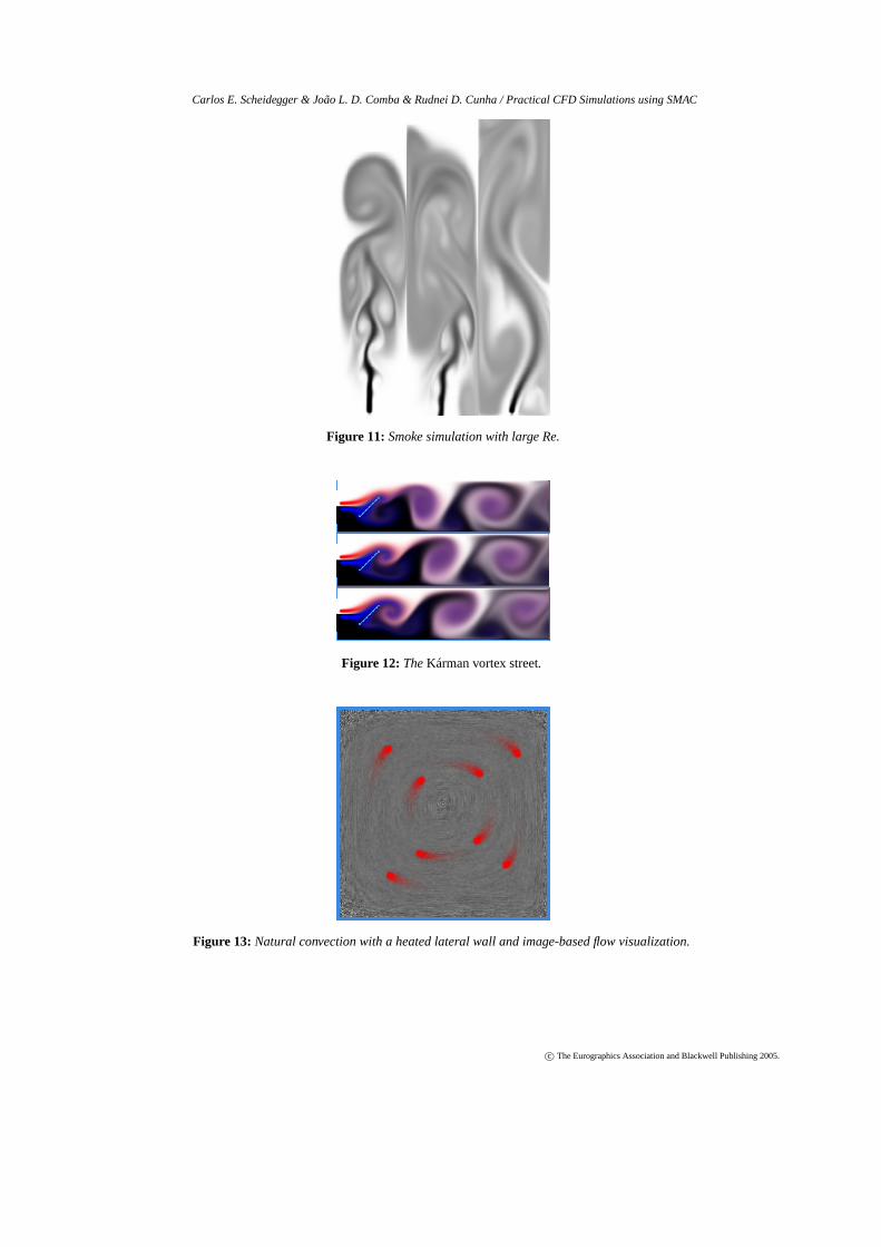
The reference CPU implementation didn’t allow for gen-eral domains, so for that part of the implementation, we hadto rely on qualitative measurements. For example, we expectvortices around corners with high speed fluid, and we cansee this in Figure9. Some well-known phenomena, such asthe Kárman vortex street[GDN98], were also experiencedin our software, in accordance to experimental results. SeeFigure12.



Figure 7: GPU-CPU ratio timings

6.2. CFD Simulation Cases

We tested our solution with several other CFD classic prob-lems discussed in [GDN98]. The simulations and their mainparameters are listed below, as well as pointers to corre-sponding figures:

• Lid-Driven Cavity: Square container filled with fluid is af-fected by the movement of the lid along a given constantvelocity. We used a 256×256 grid, withRe= 10000. Theexpected counter-eddies in the corner for largeRecan beseen on the left image of Figure8. We show a similarsimulation (Re= 1000) with our IBFV-based visualiza-tion tool (right image of Figure8). Notice how we canclearly spot the relative flow velocity and vorticity fromthe noise patterns.

• Domain with Obstacles: Square container filled with ob-stacles, with a single fluid entry and two exits. We used a128×128 grid, withRe= 1000, with inflow in the lowerwest, outflow everywhere else. (left image of Figure9).We also show a similar simulation (64× 64, Re= 100)using our IBFV-based visualization tool (right image ofFigure9). Notice how the global behavior of the fluid iscaptured, even where there’s no ink splats.

• Wind tunnel mock-up: This experiment simulates windtunnel mockup conditions with inflow fluid coming fromthe east, around an object resembling a vehicle, and out-flow in the east (Figure10). We used a 256× 64 grid,Re= 100.

• Smoke Simulation: 128×1024. In this experiment we ob-serve the effects on using large Reynold numbers, gener-ating smoke-like vector trails. We used a 128×1024 grid,with Re= 10000, inflow in the south, outflow in the north(Figure11).

• Flow Past an Obstacle: In this experiment we considerflow past a simple obstacle. For Reynold numbers above40, a Kárman vortex street effect can be seen on the trail ofvertices. We used a 256×64 grid,Re= 1000, with inflowin the west, outflow in the east (Figure12).

• Natural Convection with Heated Lateral Wall. In this ex-periment we have a square container with a heated leftlateral wall, and no-slip boundary conditions everywhere.The temperature difference drives fluid movement. Weused a 64×64 grid, withPr = 7,Re= 985.7,β = 2.1e−4and gravity componentsgx = 0 andgy=-9.706e-2. Notethe central vertex and expected circular fluid movement(Figure13).

7. Analysis

The GPU achieves top performance when doing simple cal-culations on massive amounts of data, and this is the case inour algorithm. Most of the computation is done on the GPU.The CPU only orchestrates the different GPU programs andbuffers, adjusts the timestep and determines the convergenceof the Poisson equation.

Measuring the amount of time taken in each part of our al-gorithm, we noticed that more than 95% percent of the timewas spent solving the Poisson equation. This was the mainmotivation for the exponential backoff residual calculationstep. This change doubled the overall performance.

We could have implemented a conjugated gradient solver,but since this method requires two dot products at eachtimestep, additional reductions would need to be performed(which is a slower operation). Alternatively, we could haveused a multigrid solver for the Poisson equation, such as theone developed by Goodnight et al. [GWL∗03]. We chose notto do so because we did not have a suitable CPU multigridcode to compare to, and we did not want to skew the re-sults in either way. In addition, this solver requires a moreinvolved treatment of boundary conditions, specially in com-plex environments with several obstacles.

In the simulation depicted in Figure1, we have a 1024×128 grid, and the simulation runs at approximately 20 framesper second in the NV40, allowing real-time visualization andinteraction.

8. Future Work and Conclusion

The Navier-Stokes GPU solver shown here can be easily ex-tended to three dimensions. Theuv andFG pbufferswouldhave to hold an additional channel. Additionally, we can’tuse 3D textures aspbuffers, so the texture layout would prob-ably follow [HISL03]. The fragment programs would notfundamentally change, and the overall algorithm structurewould stay the same.

A more ambitious change is to incorporate free bound-ary value problems to our solver. In this class of problems,we have to determine both the velocity field of the fluid andthe interface between the fluid and the exterior (for sloshingfluid simulations, for example). The approach that is pro-posed in the SMAC algorithm is to, starting with a knownfluid domain, place particles throughout the domain and then



displace them according to the velocity field. At the nexttimestep, the algorithm checks whether any particles arrivedin cells that had no fluid. These cells are then appropri-ately marked, and the simulation continues. We can’t do thatdirectly on the GPU, because that would require a scatteroperation. A possible solution is to use thevolume-of-fluidmethod [GDN98]. The volume-of-fluid method keeps trackof the fraction of the fluid that leave the cells through theedges. This way, all cells that are partially filled are markedas border cells, the ones completely filled are marked as fluidcells, and the ones without any fluid are marked as emptycells. Such a scheme could be implemented using GPUs,since the calculation of fluid transfer between cells can bedone for each cell individually, without having to write to ar-bitrary locations. However, this remains to be implemented.

Nevertheless, we have shown that the GPU is a viablecomputing engine for the complete solution of the Navier-Stokes via a explicit solver, suitable for engineering con-texts. Our solution takes advantage of the streaming natureof the GPU and minimizes the CPU/GPU interaction, result-ing in the high performances reported. We hope that the factthat GPU performance growth is largely outpacing the CPUwill serve as an additional motivation for the implementationof other similar applications.

9. Acknowledgments

The authors thank NVIDIA for providing the graphics hard-ware used in this paper, specially the NV40 referenceboard and drivers. The work of Carlos Eduardo Scheideggerhas been partially supported by National Science Founda-tion under grants CCF-0401498, EIA-0323604, and OISE-0405402.

References

[BFGS03] BOLZ J., FARMER I., GRINSPUN E.,SCHRÖDER P.: Sparse matrix solvers on the gpu:Conjugate gradients and multigrid.ACM Transactions onGraphics (Proceedings of SIGGRAPH 2003)(2003).

[BFH∗04] BUCK I., FOLEY T., HORN D., SUGERMAN

J., FATAHALIAN K., HOUSTON M., HANRAHAN P.:Brook for gpus: Stream computing on graphics hard-ware. ACM Transactions on Graphics (Proceedings ofSIGGRAPH 2004)(2004).

[CDPS03] COMBA J., DIETRICH C., PAGOT C., SCHEI-DEGGER C.: Computation on gpus: From a pro-grammable pipeline to an efficient stream processor.Re-vista de Informática Teórica e Aplicada X, 2 (2003).

[CL03] CABRAL B., LEEDOM L.: Imaging vector fieldsusing line integral convolution. InProceedings of SIG-GRAPH(2003).

[Cor05] CORPORATION N.: OpenGL ExtensionSpecifications. Web site last visited on June 1st,

2005, 2005, ch. http://developer.nvidia.com/ ob-ject/nvidia_opengl_specs.html.

[GDN98] GRIEBEL M., DORNSEIFERT., NEUNHOFFER

T.: Numerical Simulation in Fluid Dynamics. SIAM,1998.

[GRLM03] GOVINDARAJU N., REDON S., LIN M.,MANOCHA D.: Interactive collision detection be-tween complex models in large environments usinggraphics hardware. InProceedings of the Eurograph-ics/SIGGRAPH Graphics Hardware Workshop(2003).

[GWL∗03] GOODNIGHT N., WOOLLEY C., LEWIN G.,LUEBKE D., HUMPHREYS G.: Multigrid solver forboundary-value problems using programmable graph-ics hardware. InProceedings of the Eurograph-ics/SIGGRAPH Graphics Hardware Workshop(2003).

[HCSL02] HARRIS M., COOMBE G., SCHEUERMANN

T., LASTRA A.: Physically-based visual simulation ongraphics hardware. InProceedings of the Eurograph-ics/SIGGRAPH Graphics Hardware Workshop(2002).

[HISL03] HARRIS M., III W. B., SCHEUERMANN T.,LASTRA A.: Simulation of cloud dynamics on graph-ics hardware. InProceedings of the Eurograph-ics/SIGGRAPH Graphics Hardware Workshop(2003).

[HMG03] HILLESLAND K., MOLINOV S., GRZESCZUK

R.: Nonlinear optimization framework for image-basedmodeling on programmable graphics hardware.ACMTransactions on Graphics (Proceedings of SIGGRAPH2003(2003).

[KI99] KEDEM G., ISHIHARA Y.: Brute force attack onunix passwords with simd computer. InProceedings ofthe 8th USENIX Security Symposium, 1999(1999).

[KW03] KRÜGER J., WESTERMANN R.: Linear alge-bra operators for gpu implementation of numerical algo-rithms. ACM Transactions on Graphics (Proceedings ofSIGGRAPH 2003)(2003).

[LM01] LARSEN E., MCCALLISTER D.: Fast matrixmultiplies using graphics hardware. InSupercomputing2001(2001).

[PBMH02] PURCELL T., BUCK I., MARK W., HANRA-HAN P.: Ray tracing on programmable graphics hard-ware. ACM Transactions on Graphics (Proceedings ofSIGGRAPH 2002)(2002).

[Sta99] STAM J.: Stable fluids. ACM Transactions onGraphics (Proceedings of SIGGRAPH 1999(1999).

[vW02] VAN WIJK J.: Image-based flow visualization.ACM Transaction on Graphics (Proceedings of SIG-GRAPH 2002)(2002).

[WGE03] WEISKOPF D., G. ERLEBACHER T. E.: Atexture-based framework for spacetime-coherent visual-ization of time-dependent vector fields. InIEEE Visual-ization 2003(2003).



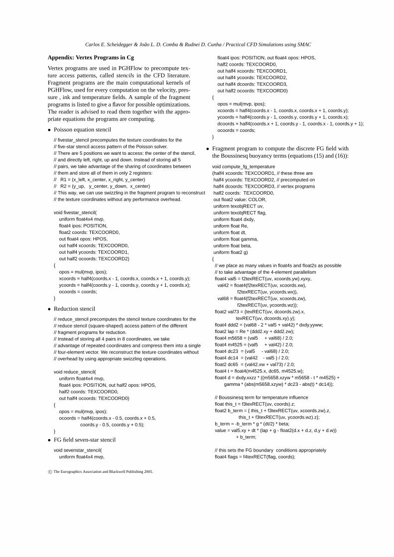
Appendix: Vertex Programs in Cg

Vertex programs are used in PGHFlow to precompute tex-ture access patterns, calledstencils in the CFD literature.Fragment programs are the main computational kernels ofPGHFlow, used for every computation on the velocity, pres-sure , ink and temperature fields. A sample of the fragmentprograms is listed to give a flavor for possible optimizations.The reader is advised to read them together with the appro-priate equations the programs are computing.

• Poisson equation stencil

// fivestar_stencil precomputes the texture coordinates for the// five-star stencil access pattern of the Poisson solver.// There are 5 positions we want to access: the center of the stencil,// and directly left, right, up and down. Instead of storing all 5// pairs, we take advantage of the sharing of coordinates between// them and store all of them in only 2 registers:// R1 = (x_left, x_center, x_right, y_center)// R2 = (y_up, y_center, y_down, x_center)// This way, we can use swizzling in the fragment program to reconstruct// the texture coordinates without any performance overhead.

void fivestar_stencil(uniform float4x4 mvp,float4 ipos: POSITION,float2 coords: TEXCOORD0,out float4 opos: HPOS,out half4 xcoords: TEXCOORD0,out half4 ycoords: TEXCOORD1,out half2 ocoords: TEXCOORD2)

{opos = mul(mvp, ipos);xcoords = half4(coords.x - 1, coords.x, coords.x + 1, coords.y);ycoords = half4(coords.y - 1, coords.y, coords.y + 1, coords.x);ocoords = coords;

}

• Reduction stencil

// reduce_stencil precomputes the stencil texture coordinates for the// reduce stencil (square-shaped) access pattern of the different// fragment programs for reduction.// Instead of storing all 4 pairs in 8 coordinates, we take// advantage of repeated coordinates and compress them into a single// four-element vector. We reconstruct the texture coordinates without// overhead by using appropriate swizzling operations.

void reduce_stencil(uniform float4x4 mvp,float4 ipos: POSITION, out half2 opos: HPOS,half2 coords: TEXCOORD0,out half4 ocoords: TEXCOORD0)

{opos = mul(mvp, ipos);ocoords = half4(coords.x - 0.5, coords.x + 0.5,

coords.y - 0.5, coords.y + 0.5);}

• FG field seven-star stencil

void sevenstar_stencil(uniform float4x4 mvp,

float4 ipos: POSITION, out float4 opos: HPOS,half2 coords: TEXCOORD0,out half4 xcoords: TEXCOORD1,out half4 ycoords: TEXCOORD2,out half4 dcoords: TEXCOORD3,out half2 ocoords: TEXCOORD0)

{opos = mul(mvp, ipos);xcoords = half4(coords.x - 1, coords.x, coords.x + 1, coords.y);ycoords = half4(coords.y - 1, coords.y, coords.y + 1, coords.x);dcoords = half4(coords.x + 1, coords.y - 1, coords.x - 1, coords.y + 1);ocoords = coords;

}

• Fragment program to compute the discrete FG field withthe Boussinesq buoyancy terms (equations (15) and (16)):

void compute_fg_temperature(half4 xcoords: TEXCOORD1, // these three arehalf4 ycoords: TEXCOORD2, // precomputed onhalf4 dcoords: TEXCOORD3, // vertex programshalf2 coords: TEXCOORD0,out float2 value: COLOR,uniform texobjRECT uv,uniform texobjRECT flag,uniform float4 dxdy,uniform float Re,uniform float dt,uniform float gamma,uniform float beta,uniform float2 g)

{// we place as many values in float4s and float2s as possible// to take advantage of the 4-element parallelismfloat4 val5 = f2texRECT(uv, xcoords.yw).xyxy,

val42 = float4(f2texRECT(uv, xcoords.xw),f2texRECT(uv, ycoords.wx)),

val68 = float4(f2texRECT(uv, xcoords.zw),f2texRECT(uv, ycoords.wz));

float2 val73 = {texRECT(uv, dcoords.zw).x,texRECT(uv, dcoords.xy).y};

float4 ddd2 = (val68 - 2 * val5 + val42) * dxdy.yyww;float2 lap = Re * (ddd2.xy + ddd2.zw);float4 m5658 = (val5 + val68) / 2.0;float4 m4525 = (val5 + val42) / 2.0;float4 dc23 = (val5 - val68) / 2.0;float4 dc14 = (val42 - val5 ) / 2.0;float2 dc65 = (val42.xw + val73) / 2.0;float4 t = float4(m4525.x, dc65, m4525.w);float4 d = dxdy.xxzz * ((m5658.xzyw * m5658 - t * m4525) +

gamma * (abs(m5658.xzyw) * dc23 - abs(t) * dc14));

// Boussinesq term for temperature influencefloat this_t = f3texRECT(uv, coords).z;float2 b_term = { this_t + f3texRECT(uv, xcoords.zw).z,

this_t + f3texRECT(uv, ycoords.wz).z};b_term = -b_term * g * (dt/2) * beta;value = val5.xy + dt * (lap + g - float2(d.x + d.z, d.y + d.w))

+ b_term;

// this sets the FG boundary conditions appropriatelyfloat4 flags = f4texRECT(flag, coords);



if (flags.y == 0) value.x = 0;if (flags.w == 0) value.y = 0;

}

• Jacobi relaxation: Most used fragment program, becausethe time to solve the Poisson equation dominates the totalrunning time. Notice that there are a lot of obscure tech-niques to take advantage of the 4-way parallelism of thefragment processor.

void jacobi_step(half4 xcoords: TEXCOORD0,half4 ycoords: TEXCOORD1,half2 coords: TEXCOORD2,out float value: COLOR,uniform texobjRECT fg,uniform texobjRECT p_old,uniform texobjRECT neighbors,// z=0, so we can throw .z of dotted vector awayuniform float3 one_over_dxdt_dydt,uniform float2 dxdy) // { 1/(dx*dx), 1/(dy*dy) }

{float4 nsew = 1 - f4texRECT(neighbors, xcoords.yw);// 4 multiplies with one instructionnsew *= dxdy.xxyy;

float4 val4628;val4628.x = f1texRECT(p_old, xcoords.xw);val4628.y = f1texRECT(p_old, xcoords.zw);val4628.z = f1texRECT(p_old, ycoords.wx);val4628.w = f1texRECT(p_old, ycoords.wz);

// 4 multiplies with one instructionval4628 *= nsew.wzyx;

// fg only stores usely r and g, but we dot it// with (...,...,0) so b is thrown away// We do this because there is no dot2 in Cg, only dot3.float3 fg5 = f3texRECT(fg, xcoords.yw);fg5.x -= f2texRECT(fg, xcoords.xw).x;fg5.y -= f2texRECT(fg, ycoords.wx).y;

// 4 multiplies and 3 adds in one instructionfloat factor = dot(float4(1,1,1,1), nsew);

// 2 multiplies and 1 add in one instructionfloat rhs = dot(fg5, one_over_dxdt_dydt);if (factor == 0.0)

value = 0;else {

// 4 multiplies and 3 adds in one instructionvalue = 1/factor * (dot(float4(1,1,1,1), val4628) - rhs);

}}

• Ink advection: main part of ink advection fragment pro-grams. We omit auxiliary functions such as the linear in-terpolating texture lookups.

void ink_advection(float2 coords: TEXCOORD0,out float4 value: COLOR,

uniform float dt,uniform float supersample,uniform float velscale,uniform float2 dxdy,uniform samplerRECT uv,uniform samplerRECT ink,uniform samplerRECT noise1,uniform samplerRECT noise2,uniform float noise_alpha,uniform float noise_modulate)

{float2 offset = fmod(coords, 1);float2 correctionx = float2(offset.x < 0.5 ? 0 : -1, 0);float2 correctiony = float2(0, offset.y < 0.5 ? 0 : -1);

float2 offsetv = offset + correctionx + float2(1, 0);float2 offsetu = offset + correctiony + float2(0, 1);

// staggeredbilerp is a bilinear interpolating texture lookup that takes// into account the staggered setup for u and vfloat u = staggered_bilerp_lookup(uv, coords + correctionx, offsetu).x;float v = staggered_bilerp_lookup(uv, coords + correctiony, offsetv).y;

// This is a lagrangian backward step in time, so that ink advection// becomes a gather op instead of a scatter op.// velscale is used to increase speeds for interactive visualizationfloat2 direction = float2(u,v) * velscale;

coords -= dt * direction / dxdy;coords *= supersample;value = bilerp_lookup(ink, coords);

// modulate noise with a sawtooth profile.float4 noise1_value = texRECT(noise1, coords);float4 noise2_value = texRECT(noise2, coords);float t1 = fmod(noise_modulate,1), t2 = 1 - t1;float4 noise_value = t1 * noise1_value + t2 * noise2_value;

// interpolate noise with previous ink valuesvalue = (1-noise_alpha) * value + noise_alpha * noise_value;

}



Figure 8: Lid-driven cavity, visualized with ink field and IBFV.

Figure 9: Domain with obstacles, visualized with ink field and IBFV.

Figure 10: Wind tunnel mock-up.



Figure 11: Smoke simulation with large Re.

Figure 12: TheKárman vortex street.

Figure 13: Natural convection with a heated lateral wall and image-based flow visualization.


practical cfd simulations on programmable graphics ...comba/papers/2005/smac-cgf.pdf · volume 0...

Documents