Practical Bayesian model evaluation using leave-one-out cross-validation andWAIC∗

Aki Vehtari† Andrew Gelman‡ Jonah Gabry‡

29 June 2016

Abstract

Leave-one-out cross-validation (LOO) and the widely applicable information criterion (WAIC)are methods for estimating pointwise out-of-sample prediction accuracy from a fitted Bayesianmodel using the log-likelihood evaluated at the posterior simulations of the parameter values.LOO and WAIC have various advantages over simpler estimates of predictive error such asAIC and DIC but are less used in practice because they involve additional computational steps.Here we lay out fast and stable computations for LOO and WAIC that can be performed usingexisting simulation draws. We introduce an efficient computation of LOO using Pareto-smoothedimportance sampling (PSIS), a new procedure for regularizing importance weights. AlthoughWAIC is asymptotically equal to LOO, we demonstrate that PSIS-LOO is more robust in thefinite case with weak priors or influential observations. As a byproduct of our calculations, wealso obtain approximate standard errors for estimated predictive errors and for comparing ofpredictive errors between two models. We implement the computations in an R package calledloo and demonstrate using models fit with the Bayesian inference package Stan.

Keywords: Bayesian computation, leave-one-out cross-validation (LOO), K-fold cross-valida-tion, widely applicable information criterion (WAIC), Stan, Pareto smoothed importance sampling(PSIS)

1. Introduction

After fitting a Bayesian model we often want to measure its predictive accuracy, for its own sake or for

purposes of model comparison, selection, or averaging (Geisser and Eddy, 1979, Hoeting et al., 1999,

Vehtari and Lampinen, 2002, Ando and Tsay, 2010, Vehtari and Ojanen, 2012). Cross-validation

and information criteria are two approaches to estimating out-of-sample predictive accuracy using

within-sample fits (Akaike, 1973, Stone, 1977). In this article we consider computations using the

log-likelihood evaluated at the usual posterior simulations of the parameters. Computation time for

the predictive accuracy measures should be negligible compared to the cost of fitting the model and

obtaining posterior draws in the first place.

Exact cross-validation requires re-fitting the model with different training sets. Approximate

leave-one-out cross-validation (LOO) can be computed easily using importance sampling (IS; Gelfand,

Dey, and Chang, 1992, Gelfand, 1996) but the resulting estimate is noisy, as the variance of the

importance weights can be large or even infinite (Peruggia, 1997, Epifani et al., 2008). Here we

propose to use Pareto smoothed importance sampling (PSIS), a new approach that provides a more

accurate and reliable estimate by fitting a Pareto distribution to the upper tail of the distribution

of the importance weights. PSIS allows us to compute LOO using importance weights that would

otherwise be unstable.

WAIC (the widely applicable or Watanabe-Akaike information criterion; Watanabe, 2010) can

be viewed as an improvement on the deviance information criterion (DIC) for Bayesian models. DIC

∗To appear in Statistics and Computing. We thank Bob Carpenter, Avraham Adler, Joona Karjalainen, SeanRaleigh, Sumio Watanabe, and Ben Lambert for helpful comments, Juho Piironen for R help, Tuomas Sivula forPython port, and the U.S. National Science Foundation, Institute of Education Sciences, and Office of Naval Researchfor partial support of this research.†Helsinki Institute for Information Technology HIIT, Department of Computer Science, Aalto University, Finland.‡Department of Statistics, Columbia University, New York.

has gained popularity in recent years, in part through its implementation in the graphical modeling

package BUGS (Spiegelhalter, Best, et al., 2002; Spiegelhalter, Thomas, et al., 1994, 2003), but it is

known to have some problems, which arise in part from not being fully Bayesian in that it is based

on a point estimate (van der Linde, 2005, Plummer, 2008). For example, DIC can produce negative

estimates of the effective number of parameters in a model and it is not defined for singular models.

WAIC is fully Bayesian in that it uses the entire posterior distribution, and it is asymptotically

equal to Bayesian cross-validation. Unlike DIC, WAIC is invariant to parametrization and also

works for singular models.

Although WAIC is asymptotically equal to LOO, we demonstrate that PSIS-LOO is more robust

in finite case with weak priors or influential observations. We provide diagnostics for both PSIS-LOO

and WAIC which tell when these approximations are likely to have large errors and computationally

more intensive methods such as K-fold cross-validation should be used. Fast and stable computation

and diagnostics for PSIS-LOO allows safe use of this new method in routine statistical practice. As

a byproduct of our calculations, we also obtain approximate standard errors for estimated predictive

errors and for the comparison of predictive errors between two models.

We implement the computations in a package for R (R Core Team, 2016) called loo (Vehtari,

Gelman, and Gabry, 2016) and demonstrate using models fit with the Bayesian inference package

Stan (Stan Development Team, 2016a, b).1 All the computations are fast compared to the typical

time required to fit the model in the first place. Although the examples provided in this paper all

use Stan, the loo package is independent of Stan and can be used with models estimated by other

software packages or custom user-written algorithms.

2. Estimating out-of-sample pointwise predictive accuracy using posterior simulations

Consider data y1, . . . , yn, modeled as independent given parameters θ; thus p(y|θ) =∏ni=1 p(yi|θ).

This formulation also encompasses latent variable models with p(yi|fi, θ), where fi are latent

variables. Also suppose we have a prior distribution p(θ), thus yielding a posterior distribution

p(θ|y) and a posterior predictive distribution p(y|y) =∫p(yi|θ)p(θ|y)dθ. To maintain comparability

with the given dataset and to get easier interpretation of the differences in scale of effective number

of parameters, we define a measure of predictive accuracy for the n data points taken one at a time:

elpd = expected log pointwise predictive density for a new dataset

=n∑

i=1

∫pt(yi) log p(yi|y)dyi, (1)

where pt(yi) is the distribution representing the true data-generating process for yi. The pt(yi)’s

are unknown, and we will use cross-validation or WAIC to approximate (1). In a regression, these

distributions are also implicitly conditioned on any predictors in the model. See Vehtari and Ojanen

(2012) for other approaches to approximating pt(yi) and discussion of alternative prediction tasks.

Instead of the log predictive density log p(yi|y), other utility (or cost) functions u(p(y|y), y) could

be used, such as classification error. Here we take the log score as the default for evaluating the

predictive density (Geisser and Eddy, 1979, Bernardo and Smith, 1994, Gneiting and Raftery, 2007).

1 The loo R package is available from CRAN and https://github.com/stan-dev/loo. The corresponding codefor Matlab, Octave, and Python is available at https://github.com/avehtari/PSIS.

2

A helpful quantity in the analysis is

lpd = log pointwise predictive density

=

n∑

i=1

log p(yi|y) =

n∑

i=1

log

∫p(yi|θ)p(θ|y)dθ. (2)

The lpd of observed data y is an overestimate of the elpd for future data (1). To compute the lpd in

practice, we can evaluate the expectation using draws from ppost(θ), the usual posterior simulations,

which we label θs, s = 1, . . . , S:

lpd = computed log pointwise predictive density

=n∑

i=1

log

(1

S

S∑

s=1

p(yi|θs)). (3)

2.1. Leave-one-out cross-validation

The Bayesian LOO estimate of out-of-sample predictive fit is

elpdloo =

n∑

i=1

log p(yi|y−i), (4)

where

p(yi|y−i) =

∫p(yi|θ)p(θ|y−i)dθ (5)

is the leave-one-out predictive density given the data without the ith data point.

Raw importance sampling. As noted by Gelfand, Dey, and Chang (1992), if the n points are

conditionally independent in the data model we can then evaluate (5) with draws θs from the full

posterior p(θ|y) using importance ratios

rsi =1

p(yi|θs)∝ p(θs|y−i)

p(θs|y)(6)

to get the importance sampling leave-one-out (IS-LOO) predictive distribution,

p(yi|y−i) ≈∑S

s=1 rsi p(yi|θs)∑Ss=1 r

si

. (7)

Evaluating this LOO log predictive density at the held-out data point yi, we get

p(yi|y−i) ≈1

1S

∑Ss=1

1p(yi|θs)

. (8)

However, the posterior p(θ|y) is likely to have a smaller variance and thinner tails than the leave-one-

out distributions p(θ|y−i), and thus a direct use of (8) induces instability because the importance

ratios can have high or infinite variance.

For simple models the variance of the importance weights may be computed analytically. The

necessary and sufficient conditions for the variance of the case-deletion importance sampling weights

to be finite for a Bayesian linear model are given by Peruggia (1997). Epifani et al. (2008) extend the

3

analytical results to generalized linear models and non-linear Michaelis-Menten models. However,

these conditions can not be computed analytically in general.

Koopman et al. (2009) propose to use the maximum likelihood fit of the generalized Pareto

distribution to the upper tail of the distribution of the importance ratios and use the fitted parameters

to form a test for whether the variance of the importance ratios is finite. If the hypothesis test

suggests the variance is infinite then they abandon importance sampling.

Truncated importance sampling. Ionides (2008) proposes a modification of importance sam-

pling where the raw importance ratios rs are replaced by truncated weights

ws = min(rs,√Sr), (9)

where r = 1S

∑Ss=1 r

s. Ionides (2008) proves that the variance of the truncated importance sampling

weights is guaranteed to be finite, and provides theoretical and experimental results showing that

truncation using the threshold√Sr gives an importance sampling estimate with a mean square error

close to an estimate with a case specific optimal truncation level. The downside of the truncation is

that it introduces a bias, which can be large as we demonstrate in our experiments.

Pareto smoothed importance sampling. We can improve the LOO estimate using Pareto

smoothed importance sampling (PSIS; Vehtari and Gelman, 2015), which applies a smoothing

procedure to the importance weights. We briefly review the motivation and steps of PSIS here,

before moving on to focus on the goals of using and evaluating predictive information criteria.

As noted above, the distribution of the importance weights used in LOO may have a long right

tail. We use the empirical Bayes estimate of Zhang and Stephens (2009) to fit a generalized Pareto

distribution to the tail (20% largest importance ratios). By examining the shape parameter k of

the fitted Pareto distribution, we are able to obtain sample based estimates of the existence of the

moments (Koopman et al, 2009). This extends the diagnostic approach of Peruggia (1997) and

Epifani et al. (2008) to be used routinely with IS-LOO for any model with a factorizing likelihood.

Epifani et al. (2008) show that when estimating the leave-one-out predictive density, the central

limit theorem holds if the distribution of the weights has finite variance. These results can be

extended via the generalized central limit theorem for stable distributions. Thus, even if the variance

of the importance weight distribution is infinite, if the mean exists then the accuracy of the estimate

improves as additional posterior draws are obtained.

When the tail of the weight distribution is long, a direct use of importance sampling is sensitive

to one or few largest values. By fitting a generalized Pareto distribution to the upper tail of the

importance weights, we smooth these values. The procedure goes as follows:

1. Fit the generalized Pareto distribution to the 20% largest importance ratios rs as computed

in (6). The computation is done separately for each held-out data point i. In simulation

experiments with thousands and tens of thousands of draws, we have found that the fit is not

sensitive to the specific cutoff value (for a consistent estimation, the proportion of the samples

above the cutoff should get smaller when the number of draws increases).

2. Stabilize the importance ratios by replacing the M largest ratios by the expected values of

the order statistics of the fitted generalized Pareto distribution

F−1(z − 1/2

M

), z = 1, . . . ,M,

4

where M is the number of simulation draws used to fit the Pareto (in this case, M = 0.2S)

and F−1 is the inverse-CDF of the generalized Pareto distribution. Label these new weights

as wsi where, again, s indexes the simulation draws and i indexes the data points; thus, for

each i there is a distinct vector of S weights.

3. To guarantee finite variance of the estimate, truncate each vector of weights at S3/4wi, where

wi is the average of the S smoothed weights corresponding to the distribution holding out

data point i. Finally, label these truncated weights as wsi .

The above steps must be performed for each data point i. The result is a vector of weights

wsi , s = 1, . . . , S, for each i, which in general should be better behaved than the raw importance

ratios rsi from which they are constructed.

The results can then be combined to compute desired LOO estimates. The PSIS estimate of the

LOO expected log pointwise predictive density is

elpdpsis−loo =

n∑

i=1

log

(∑Ss=1w

si p(yi|θs)∑S

s=1wsi

). (10)

The estimated shape parameter k of the generalized Pareto distribution can be used to assess

the reliability of the estimate:

• If k < 12 , the variance of the raw importance ratios is finite, the central limit theorem holds,

and the estimate converges quickly.

• If k is between 12 and 1, the variance of the raw importance ratios is infinite but the mean

exists, the generalized central limit theorem for stable distributions holds, and the convergence

of the estimate is slower. The variance of the PSIS estimate is finite but may be large.

• If k > 1, the variance and the mean of the raw ratios distribution do not exist. The variance

of the PSIS estimate is finite but may be large.

If the estimated tail shape parameter k exceeds 0.5, the user should be warned, although in practice

we have observed good performance for values of k up to 0.7. Even if the PSIS estimate has a

finite variance, when k exceeds 0.7 the user should consider sampling directly from p(θs|y−i) for the

problematic i, use K-fold cross-validation (see Section 2.3), or use a more robust model.

The additional computational cost of sampling directly from each p(θs|y−i) is approximately the

same as sampling from the full posterior, but it is recommended if the number of problematic data

points is not too high.

A more robust model may also help because importance sampling is less likely to work well if

the marginal posterior p(θs|y) and LOO posterior p(θs|y−i) are very different. This is more likely to

happen with a non-robust model and highly influential observations. A robust model may reduce the

sensitivity to one or several highly influential observations, as we show in the examples in Section 4.

2.2. WAIC

WAIC (Watanabe, 2010) is an alternative approach to estimate the expected log pointwise predictive

density and is defined as

elpdwaic = lpd− pwaic, (11)

5

where pwaic is the estimated effective number of parameters and computed based on the definition2

pwaic =

n∑

i=1

varpost (log p(yi|θ)) , (12)

which we can calculate using the posterior variance of the log predictive density for each data point

yi, that is, V Ss=1 log p(yi|θs), where V S

s=1 represents the sample variance, V Ss=1as = 1

S−1∑S

s=1(as− a)2.

Summing over all the data points yi gives a simulation-estimated effective number of parameters,

pwaic =n∑

i=1

V Ss=1 (log p(yi|θs)) . (13)

For DIC, there is a similar variance-based computation of the number of parameters that is

notoriously unreliable, but the WAIC version is more stable because it computes the variance

separately for each data point and then takes the sum; the summing yields stability.

The effective number of parameters pwaic can be used as measure of complexity of the model,

but it should not be overinterpreted, as the original goal is to estimate the difference between lpd

and elpd. As shown by Gelman, Hwang, and Vehtari (2014) and demonstrated also in Section

4, in the case of a weak prior, pwaic can severely underestimate the difference between lpd and

elpd. For pwaic there is no similar theory as for the moments of the importance sampling weight

distribution, but based on our simulation experiments it seems that pwaic is unreliable if any of the

terms V Ss=1 log p(yi|θs) exceeds 0.4.

The different behavior of LOO and WAIC seen in the experiments can be understood by

comparing Taylor series approximations. By defining a generating function of functional cumulants,

F (α) =n∑

i=1

logEpost(p(yi|θ)α), (14)

and applying a Taylor expansion of F (α) around 0 with α = −1 we obtain an expansion of lpdloo

elpdloo = F ′(0)− 1

2F ′′(0) +

1

6F (3)(0)−

∞∑

i=4

(−1)iF (i)(0)

i!. (15)

From the definition of F (α) we get

F (0) = 0

F (1) =n∑

i=1

logEpost(p(yi|θ))

F ′(0) =

n∑

i=1

Epost(log p(yi|θ))

F ′′(0) =n∑

i=1

varpost(log p(yi|θ)). (16)

Furthermore

lpd = F (1) = F ′(0) +1

2F ′′(0) +

1

6F (3)(0) +

∞∑

i=4

F (i)(0)

i!, (17)

2In Gelman, Carlin, et al. (2013), the variance-based pwaic defined here is called pwaic 2. There is also a mean-basedformula, pwaic 1, which we do not use here.

6

and the expansion for WAIC is then

WAIC = F (1)− F ′′(0)

= F ′(0)− 1

2F ′′(0) +

1

6F (3)(0) +

∞∑

i=4

F (i)(0)

i!. (18)

The first three terms of the expansion of WAIC match the expansion of LOO, and the rest of the

terms match the expansion of lpd. Watanabe (2010) argues that, asymptotically, the latter terms

have negligible contribution and thus asymptotic equivalence with LOO is obtained. However, the

error can be significant in the case of finite n and weak prior information as shown by Gelman,

Hwang, and Vehtari (2014), and demonstrated also in Section 4. If the higher order terms are not

negligible, then WAIC is biased towards lpd. To reduce this bias it is possible to compute additional

series terms, but computing higher moments using a finite posterior sample increases the variance

of the estimate and, based on our experiments, it is more difficult to control the bias-variance

tradeoff than in PSIS-LOO. WAIC’s larger bias compared to LOO is also demonstrated by Vehtari

et al. (2016) in the case of Gaussian processes with distributional posterior approximations. In the

experiments we also demonstrate the we can use truncated IS-LOO with heavy truncation to obtain

similar bias towards lpd and similar estimate variance as in WAIC.

2.3. K-fold cross-validation

In this paper we focus on leave-one-out cross-validation and WAIC, but, for statistical and compu-

tational reasons, it can make sense to cross-validate using K << n hold-out sets. In some ways,

K-fold cross-validation is simpler than leave-one-out cross-validation but in other ways it is not.

K-fold cross-validation requires refitting the model K times which can be computationally expensive

whereas approximative LOO methods, such as PSIS-LOO, require only one evaluation of the model.

If in PSIS-LOO k > 0.7 for a few i we recommend sampling directly from each corresponding

p(θs|y−i), but if there are more than K problematic i, then we recommend checking the results

using K-fold cross-validation. Vehtari & Lampinen (2002) demonstrate cases where IS-LOO fails

(according to effective sample size estimates instead of the k diagnostic proposed here) for a large

number of i and K-fold-CV produces more reliable results.

In Bayesian K-fold cross-validation, the data are partitioned into K subsets yk, for k = 1, . . . ,K,

and then the model is fit separately to each training set y(−k), thus yielding a posterior distribution

ppost(−k)(θ) = p(θ|y(−k)). If the number of partitions is small (a typical value in the literature is

K = 10), it is not so costly to simply re-fit the model separately to each training set. To maintain

consistency with LOO and WAIC, we define predictive accuracy for each data point, so that the log

predictive density for yi, if it is in subset k, is

log p(yi|y(−k)) = log

∫p(yi|θ)p(θ|y(−k))dθ, i ∈ k. (19)

Assuming the posterior distribution p(θ|y(−k)) is summarized by S simulation draws θk,s, we calculate

its log predictive density as

elpdi = log

(1

S

S∑

s=1

p(yi|θk,s))

(20)

using the simulations corresponding to the subset k that contains data point i. We then sum to get

the estimate

elpdxval =n∑

i=1

elpdi. (21)

7

There remains a bias as the model is learning from a fraction 1K less of the data. Methods for

correcting this bias exist but are rarely used as they can increase the variance, and if K ≥ 10 the

size of the bias is typically small compared to the variance of the estimate (Vehtari and Lampinen,

2002). In our experiments, exact LOO is the same as K-fold-CV with K = N and we also analyze

the effect of this bias and bias correction in Section 4.2.

For K-fold cross-validation, if the subjects are exchangeable, that is, the order does not contain

information, then there is no need for random selection. If the order does contain information, e.g.

in survival studies the later patients have shorter follow-ups, then randomization is often useful.

In most cases we recommend partitioning the data into subsets by randomly permuting the

observations and then systemically dividing them into K subgroups. If the subjects are exchangeable,

that is, the order does not contain information, then there is no need for random selection, but if

the order does contain information, e.g. in survival studies the later patients have shorter follow-ups,

then randomization is useful. In some cases it may be useful to stratify to obtain better balance

among groups. See Vehtari and Lampinen (2002), Celisse and Arlot (2010), and Vehtari and Ojanen

(2012) for further discussion of these points.

As the data can be divided in many ways into K groups it introduces additional variance in the

estimates, which is also evident from our experiments. This variance can be reduced by repeating

K-fold-CV several times with different permutations in the data division, but this will further

increase the computational cost.

2.4. Data division

The purpose of using LOO or WAIC is to estimate the accuracy of the predictive distribution

p(yi|y). Computation of PSIS-LOO and WAIC (and AIC and DIC) is based on computing terms

log p(yi|y) = log∫p(yi|θ)p(θ|y) assuming some agreed-upon division of the data y into individual

data points yi. Although often yi will denote a single scalar observation, in the case of hierarchical

data, it may denote a group of observations. For example, in cognitive or medical studies we may

be interested in prediction for a new subject (or patient), and thus it is natural in cross-validation

to consider an approach where yi would denote all observations for a single subject and y−i would

denote the observations for all the other subjects. In theory, we can use PSIS-LOO and WAIC

in this case, too, but as the number of observations per subject increases it is more likely that

they will not work as well. The fact that importance sampling is difficult in higher dimensions

is well known and is demonstrated for IS-LOO by Vehtari and Lampinen (2002) and for PSIS by

Vehtari and Gelman (2014, Figure 5). The same problem can also be shown to hold for WAIC. If

diagnostics warn about the reliability of PSIS-LOO (or WAIC), then K-fold cross-validation can be

used by taking into account the hierarchical structure in the data when doing the data division as

demonstrated, for example, by Vehtari and Lampinen (2002).

3. Implementation in Stan

We have set up code to implement LOO, WAIC, and K-fold cross-validation in R and Stan so that

users will have a quick and convenient way to assess and compare model fits. Implementation is not

automatic, though, because of the need to compute the separate factors p(yi|θ) in the likelihood.

Stan works with the joint density and in its usual computations does not “know” which parts come

from the prior and which from the likelihood. Nor does Stan in general make use of any factorization

of the likelihood into pieces corresponding to each data point. Thus, to compute these measures of

predictive fit in Stan, the user needs to explicitly code the factors of the likelihood (actually, the

8

terms of the log-likelihood) as a vector. We can then pull apart the separate terms and compute

cross-validation and WAIC at the end, after all simulations have been collected. Sample code for

carrying out this procedure using Stan and the loo R package is provided in Appendix A. This

code can be adapted to apply our procedure in other computing languages.

Although the implementation is not automatic when writing custom Stan programs, we can

create implementations that are automatic for users of our new rstanarm R package (Gabry and

Goodrich, 2016). rstanarm provides a high-level interface to Stan that enables the user to specify

many of the most common applied Bayesian regression models using standard R modeling syntax

(e.g. like that of glm). The models are then estimated using Stan’s algorithms and the results are

returned to the user in a form similar to the fitted model objects to which R users are accustomed.

The fact For the models implemented in rstanarm, we have preprogrammed many tasks, including

computing and saving the pointwise predictive measures and importance ratios which we use to

compute WAIC and PSIS-LOO. The loo method for rstanarm models requires no additional

programming from the user after fitting a model, as we can compute all of the needed quantities

internally from the contents of the fitted model object and then pass them to the functions in the

loo package. Examples of using loo with rstanarm can be found in the rstanarm vignettes, and

we also provide an example in Appendix A.3 of this paper.

4. Examples

We illustrate with six simple examples: two examples from our earlier research in computing the

effective number of parameters in a hierarchical model, three examples that were used by Epifani et

al. (2008) to illustrate the estimation of the variance of the weight distribution, and one example

of a multilevel regression from our earlier applied research. For each example we used the Stan

default of 4 chains run for 1000 warmup and 1000 post-warmup iterations, yielding a total of

4000 saved simulation draws. With Gibbs sampling or random-walk Metropolis, 4000 is not a

large number of simulation draws. The algorithm used by Stan is Hamiltonian Monte Carlo with

No-U-Turn-Sampling (Hoffman and Gelman, 2014), which is much more efficient, and 1000 is

already more than sufficient in many real-world settings. In these examples we followed standard

practice and monitored convergence and effective sample sizes as recommended by Gelman, Carlin,

et al. (2013). We performed 100 independent replications of all experiments to obtain estimates of

variation. For the exact LOO results and convergence plots we run longer chains to obtain total of

100,000 draws (except for the radon example which is much slower to run).

4.1. Example: Scaled 8 schools

For our first example we take an analysis of an education experiment used by Gelman, Hwang, and

Vehtari (2014) to demonstrate the use of information criteria for hierarchical Bayesian models.

The goal of the study was to measure the effects of a test preparation program conducted in

eight different high schools in New Jersey. A separate randomized experiment was conducted in

each school, and the administrators of each school implemented the program in their own way.

Rubin (1981) performed a Bayesian meta-analysis, partially pooling the eight estimates toward a

common mean. The model has the form, yi ∼ N(θi, σ2i ) and θi ∼ N(µ, τ2), for i = 1, . . . , n = 8, with

a uniform prior distribution on (µ, τ). The measurements yi and uncertainties σi are the estimates

and standard errors from separate regressions performed for each school, as shown in Table 1. The

test scores for the individual students are no longer available.

This model has eight parameters but they are constrained through their hierarchical distribution

9

Estimated Standard errorSchool effect, yj of estimate, σj

A 28 15B 8 10C −3 16D 7 11E −1 9F 1 11G 18 10H 12 18

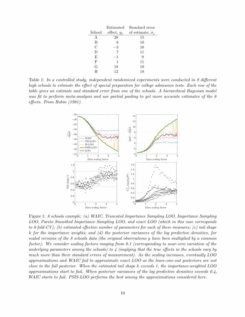
Table 1: In a controlled study, independent randomized experiments were conducted in 8 different

high schools to estimate the effect of special preparation for college admission tests. Each row of the

table gives an estimate and standard error from one of the schools. A hierarchical Bayesian model

was fit to perform meta-analysis and use partial pooling to get more accurate estimates of the 8

effects. From Rubin (1981).

0 1 2 3 4−44

−42

−40

−38

−36

−34

−32

−30

−28

Data scaling factor

elppd

WAICTIS-LOOIS-LOOPSIS-LOOLOO

0 1 2 3 40

2

4

6

8

10

12

14

Data scaling factor

lppd− elppd

0 1 2 3 40

0.2

0.4

0.6

0.8

1

1.2

Data scaling factor

Tailshap

ek

0 1 2 3 40

0.2

0.4

0.6

0.8

1

1.2

1.4

1.6

Data scaling factor

VS s=1logp(y

i|θs)

Figure 1: 8 schools example: (a) WAIC, Truncated Importance Sampling LOO, Importance Sampling

LOO, Pareto Smoothed Importance Sampling LOO, and exact LOO (which in this case corresponds

to 8-fold-CV); (b) estimated effective number of parameters for each of these measures; (c) tail shape

k for the importance weights; and (d) the posterior variances of the log predictive densities, for

scaled versions of the 8 schools data (the original observations y have been multiplied by a common

factor). We consider scaling factors ranging from 0.1 (corresponding to near-zero variation of the

underlying parameters among the schools) to 4 (implying that the true effects in the schools vary by

much more than their standard errors of measurement). As the scaling increases, eventually LOO

approximations and WAIC fail to approximate exact LOO as the leave-one-out posteriors are not

close to the full posterior. When the estimated tail shape k exceeds 1, the importance-weighted LOO

approximations start to fail. When posterior variances of the log predictive densities exceeds 0.4,

WAIC starts to fail. PSIS-LOO performs the best among the approximations considered here.

10

5 10 15 20 25 300

2

4

6

Population distribution scale τ0

RMSE

WAICTIS-LOOIS-LOOPSIS-LOOLOO

5 10 15 20 25 300

2

4

6

Population distribution scale τ0

RMSE

WAICBC-PSIS-LOOBC-LOO

5 10 15 20 25 300

2

4

6

Population distribution scale τ0

RMSE

WAIC

TIS(1/4)-LOOPSIS-LOOBC-LOOShrunk LOO

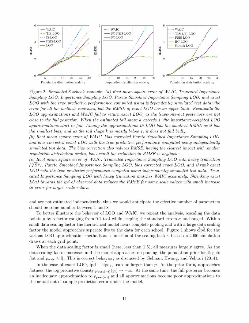
Figure 2: Simulated 8 schools example: (a) Root mean square error of WAIC, Truncated Importance

Sampling LOO, Importance Sampling LOO, Pareto Smoothed Importance Sampling LOO, and exact

LOO with the true predictive performance computed using independently simulated test data; the

error for all the methods increases, but the RMSE of exact LOO has an upper limit. Eventually the

LOO approximations and WAIC fail to return exact LOO, as the leave-one-out posteriors are not

close to the full posterior. When the estimated tail shape k exceeds 1, the importance-weighted LOO

approximations start to fail. Among the approximations IS-LOO has the smallest RMSE as it has

the smallest bias, and as the tail shape k is mostly below 1, it does not fail badly.

(b) Root mean square error of WAIC, bias corrected Pareto Smoothed Importance Sampling LOO,

and bias corrected exact LOO with the true predictive performance computed using independently

simulated test data. The bias correction also reduces RMSE, having the clearest impact with smaller

population distribution scales, but overall the reduction in RMSE is negligible.

(c) Root mean square error of WAIC, Truncated Importance Sampling LOO with heavy truncation

( 4√Sr), Pareto Smoothed Importance Sampling LOO, bias corrected exact LOO, and shrunk exact

LOO with the true predictive performance computed using independently simulated test data. Trun-

cated Importance Sampling LOO with heavy truncation matches WAIC accurately. Shrinking exact

LOO towards the lpd of observed data reduces the RMSE for some scale values with small increase

in error for larger scale values.

and are not estimated independently; thus we would anticipate the effective number of parameters

should be some number between 1 and 8.

To better illustrate the behavior of LOO and WAIC, we repeat the analysis, rescaling the data

points y by a factor ranging from 0.1 to 4 while keeping the standard errors σ unchanged. With a

small data scaling factor the hierarchical model nears complete pooling and with a large data scaling

factor the model approaches separate fits to the data for each school. Figure 1 shows elpd for the

various LOO approximation methods as a function of the scaling factor, based on 4000 simulation

draws at each grid point.

When the data scaling factor is small (here, less than 1.5), all measures largely agree. As the

data scaling factor increases and the model approaches no pooling, the population prior for θi gets

flat and pwaic ≈ p2 . This is correct behavior, as discussed by Gelman, Hwang, and Vehtari (2014).

In the case of exact LOO, lpd − elpdloo can be larger than p. As the prior for θi approaches

flatness, the log predictive density ppost(−i)(yi)→ −∞. At the same time, the full posterior becomes

an inadequate approximation to ppost(−i) and all approximations become poor approximations to

the actual out-of-sample prediction error under the model.

11

WAIC starts to fail when one of the posterior variances of the log predictive densities exceeds

0.4. LOO approximations work well even if the tail shape k of the generalized Pareto distribution

is between 12 and 1, and the variance of the raw importance ratios is infinite. The error of LOO

approximations increases with k, with a clearer difference between the methods when k > 0.7.

4.2. Example: Simulated 8 schools

In the previous example, we used exact LOO as the gold standard. In this section, we generate

simulated data from the same statistical model and compare predictive performance on independent

test data. Even when the number of observations n is fixed, as the scale of the population distribution

increases we observe the effect of weak prior information in hierarchical models discussed in the

previous section and by Gelman, Hwang, and Vehtari (2014). Comparing the error, bias and variance

of the various approximations, we find that PSIS-LOO offers the best balance.

For i = 1, . . . , n = 8, we simulate θ0,i ∼ N(µ0, τ20 ) and yi ∼ N(θ0,i, σ

20,i), where we set σ0,i = 10,

µ0 = 0, and τ0 ∈ {1, 2, . . . , 30}. The simulated data is similar to the real 8 schools data, for which

the empirical estimate is τ ≈ 10. For each value of τ0 we generate 100 training sets of size 8 and one

test data set of size 1000. Posterior inference is based on 4000 draws for each constructed model.

Figure 2a shows the root mean square error (RMSE) for the various LOO approximation

methods as a function of τ0, the scale of the population distribution. When τ0 is large all of the

approximations eventually have ever increasing RMSE, while exact LOO has an upper limit. For

medium scales the approximations have smaller RMSE than exact LOO. As discussed later, this is

explained by the difference in the variance of the estimates. For small scales WAIC has slightly

smaller RMSE than the other methods (including exact LOO).

Watanabe (2010) shows that WAIC gives an asymptotically unbiased estimate of the out-of-

sample prediction error—this does not hold for hierarchical models with weak prior information

as shown by Gelman, Hwang, and Vehtari (2014)—but exact LOO is slightly biased as the LOO

posteriors use only n− 1 observations. WAIC’s different behavior can be understood through the

truncated Taylor series correction to the lpd, that is, not using the entire series will bias it towards

lpd (see Section 2.2). The bias in LOO is negligible when n is large, but with small n it can be be

larger.

Figure 2b shows RMSE for the bias corrected LOO approximations using the first order correction

of Burman (1989). For small scales the error of bias corrected LOOs is smaller than WAIC. When

the scale increases the RMSEs are close to the non-corrected versions. Although the bias correction

is easy to compute, the difference in accuracy is negligible for most applications.

We shall discuss Figure 2c in a moment, but first consider Figure 3, which shows the RMSE

of the approximation methods and the lpd of observed data decomposed into bias and standard

deviation. All methods (except the lpd of observed data) have small biases and variances with small

population distribution scales. Bias corrected exact LOO has practically zero bias for all scale values

but the highest variance. When the scale increases the LOO approximations eventually fail and

bias increases. As the approximations start to fail, there is a certain region where implicit shrinkage

towards the lpd of observed data decelerates the increase in RMSE as the variance is reduced, even

if the bias continues to grow.

If the goal were to minimize the RMSE for smaller and medium scales, we could also shrink

exact LOO and increase shrinkage in approximations. Figure 2c shows the RMSE of the LOO

approximations with two new choices. Truncated Importance Sampling LOO with very heavy

truncation (to 4√Sr) closely matches the performance of WAIC. In the experiments not included

here, we also observed that adding more correct Taylor series terms to WAIC will make it behave

12

5 10 15 20 25 300

2

4

6

Population distribution scale τ0

Bias

WAICPSIS-LOOBC-LOOLPD

5 10 15 20 25 300

0.5

1

1.5

2

2.5

Population distribution scale τ0

Std

WAICPSIS-LOOBC-LOOLPD

Figure 3: Simulated 8 schools example: (a) Absolute bias of WAIC, Pareto Smoothed Importance

Sampling LOO, bias corrected exact LOO, and the lpd (log predictive density) of observed data with

the true predictive performance computed using independently simulated test data; (b) standard

deviation for each of these measures; All methods except the lpd of observed data have small biases

and variances with small population distribution scales. When the scale increases the bias of WAIC

increases faster than the bias of the other methods (except the lpd of observed data). Bias corrected

exact LOO has practically zero bias for all scale values. WAIC and Pareto Smoothed Importance

Sampling LOO have lower variance than exact LOO, as they are shrunk towards the lpd of observed

data, which has the smallest variance with all scales.

similar to Truncated Importance Sampling with less truncation (see discussion of Taylor series

expansion in Section 2.2). Shrunk exact LOO (α · elpdloo + (1− α) · lpd, with α = 0.85 chosen by

hand for illustrative purposes only) has a smaller RMSE for small and medium scale values as the

variance is reduced, but the price is increased bias at larger scale values.

If the goal is robust estimation of predictive performance, then exact LOO is the best general

choice because the error is limited even in the case of weak priors. Of the approximations, PSIS-LOO

offers the best balance as well as diagnostics for identifying when it is likely failing.

4.3. Example: Linear regression for stack loss data

To check the performance of the proposed diagnostic for our second example we analyze the stack

loss data used by Peruggia (1997) which is known to have analytically proven infinite variance of

one of the importance weight distributions.

The data consist of n = 21 daily observations on one outcome and three predictors pertaining to

a plant for the oxidation of ammonia to nitric acid. The outcome y is an inverse measure of the

efficiency of the plant and the three predictors x1, x2, and x3 measure rate of operation, temperature

of cooling water, and (a transformation of the) concentration of circulating acid.

Peruggia (1997) shows that the importance weights for leave-one-out cross-validation for the

data point y21 have infinite variance. Figure 4 shows the distribution of the estimated tail shapes k

and estimation errors compared to LOO in 100 independent Stan runs.3 The estimates of the tail

shape k for i = 21 suggest that the variance of the raw importance ratios is infinite, however the

generalized central limit theorem for stable distributions holds and we can still obtain an accurate

estimate of the component of LOO for this data point using PSIS.

3Smoothed density estimates were made using a logistic Gaussian process (Vehtari and Riihimaki, 2014).

13

0 5 10 15 20−0.2

0

0.2

0.4

0.6

0.8

1

1.2

i

k

0 5 10 15 20−0.4

−0.2

0

0.2

0.4

i

LOO−

PSIS-LOO

Figure 4: Stack loss example with normal errors: Distributions of (a) tail shape estimates and (b)

PSIS-LOO estimation errors compared to LOO, from 100 independent Stan runs. The pointwise

calculation of the terms in PSIS-LOO reveals that much of the uncertainty comes from a single data

point, and it could make sense to simply re-fit the model to the subset and compute LOO directly for

that point.

0 0.2 0.4 0.6 0.8 1

·105

0.8

1

1.2

Number of posterior draws

Shap

eparam

eter

kfori=

21

0 0.2 0.4 0.6 0.8 1

·105

−6.6

−6.4

−6.2

−6

−5.8

Number of posterior draws

elppdfori=

21

WAICTIS-LOOIS-LOOPSIS-LOOLOO

Figure 5: Stack loss example with normal errors: (a) Tail shape estimate and (b) LOO approximations

for the difficult point, i = 21. When more draws are obtained, the estimates converge (slowly)

following the generalized central limit theorem.

14

0 5 10 15 20−0.2

0

0.2

0.4

0.6

0.8

1

i

k

0 5 10 15 20−0.4

−0.2

0

0.2

0.4

i

LOO−

PSIS-LOO

Figure 6: Stack loss example with Student-t errors: Distributions of (a) tail shape estimates and (b)

PSIS-LOO estimation errors compared to LOO, from 100 independent Stan runs. The computations

are more stable than with normal errors (compare to Figure 4).

Figure 5 shows that if we continue sampling, the estimates for both the tail shape k and elpdi do

converge (although slowly as k is close to 1). As the convergence is slow it would be more efficient

to sample directly from p(θs|y−i) for the problematic i.

High estimates of the tail shape parameter k indicate that the full posterior is not a good

importance sampling approximation to the desired leave-one-out posterior, and thus the observation

is surprising according to the model. It is natural to consider an alternative model. We tried

replacing the normal observation model with a Student-t to make the model more robust for the

possible outlier. Figure 6 shows the distribution of the estimated tail shapes k and estimation errors

for PSIS-LOO compared to LOO in 100 independent Stan runs for the Student-t linear regression

model. The estimated tail shapes and the errors in computing this component of LOO are smaller

than with Gaussian model.

4.4. Example: Nonlinear regression for Puromycin reaction data

As a nonlinear regression example, we use the Puromycin biochemical reaction data also analyzed

by Epifani et al. (2008). For a group of cells not treated with the drug Puromycin, there are

n = 11 measurements of the initial velocity of a reaction, Vi , obtained when the concentration

of the substrate was set at a given positive value, ci. Velocity on concentration is given by the

Michaelis-Menten relation, Vi ∼ N(mci/(κ + ci), σ2). Epifani et al. (2008) show that the raw

importance ratios for observation i = 1 have infinite variance.

Figure 7 shows the distribution of the estimated tail shapes k and estimation errors compared

to LOO in 100 independent Stan runs. The estimates of the tail shape k for i = 1 suggest that the

variance of the raw importance ratios is infinite. However, the generalized central limit theorem

for stable distributions still holds and we can get an accurate estimate of the corresponding term

in LOO. We could obtain more draws to reduce the Monte Carlo error, or again consider a more

robust model.

4.5. Example: Logistic regression for leukemia survival

Our next example uses a logistic regression model to predict survival of leukemia patients past 50

weeks from diagnosis. These data were also analyzed by Epifani et al. (2008). Explanatory variables

15

0 2 4 6 8 10 12

0

0.2

0.4

0.6

0.8

1

i

Shap

eparam

eter

k

0 2 4 6 8 10 12−0.4

−0.2

0

0.2

0.4

i

LOO

−PSIS-LOO

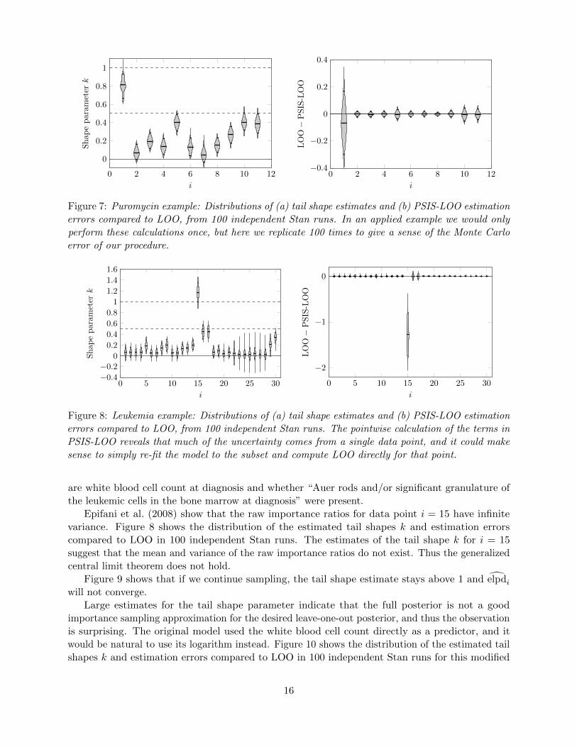
Figure 7: Puromycin example: Distributions of (a) tail shape estimates and (b) PSIS-LOO estimation

errors compared to LOO, from 100 independent Stan runs. In an applied example we would only

perform these calculations once, but here we replicate 100 times to give a sense of the Monte Carlo

error of our procedure.

0 5 10 15 20 25 30−0.4

−0.20

0.2

0.4

0.6

0.8

1

1.2

1.4

1.6

i

Shapeparameter

k

0 5 10 15 20 25 30

−2

−1

0

i

LOO

−PSIS-LOO

Figure 8: Leukemia example: Distributions of (a) tail shape estimates and (b) PSIS-LOO estimation

errors compared to LOO, from 100 independent Stan runs. The pointwise calculation of the terms in

PSIS-LOO reveals that much of the uncertainty comes from a single data point, and it could make

sense to simply re-fit the model to the subset and compute LOO directly for that point.

are white blood cell count at diagnosis and whether “Auer rods and/or significant granulature of

the leukemic cells in the bone marrow at diagnosis” were present.

Epifani et al. (2008) show that the raw importance ratios for data point i = 15 have infinite

variance. Figure 8 shows the distribution of the estimated tail shapes k and estimation errors

compared to LOO in 100 independent Stan runs. The estimates of the tail shape k for i = 15

suggest that the mean and variance of the raw importance ratios do not exist. Thus the generalized

central limit theorem does not hold.

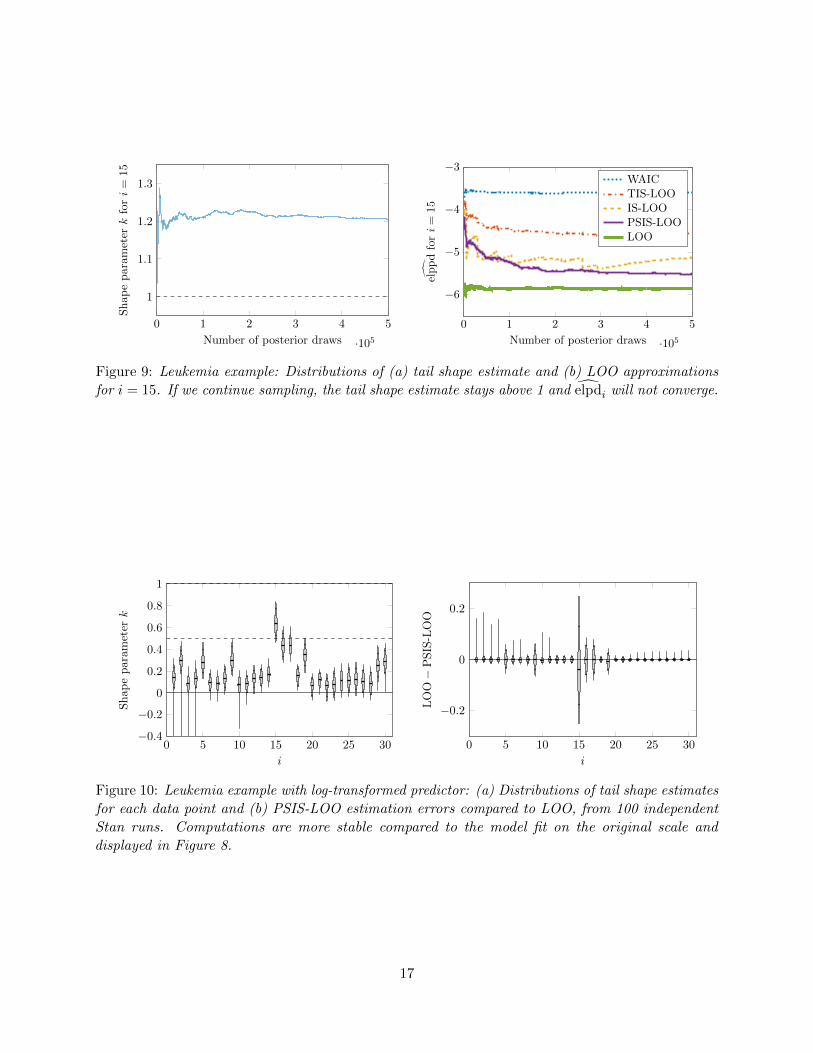
Figure 9 shows that if we continue sampling, the tail shape estimate stays above 1 and elpdiwill not converge.

Large estimates for the tail shape parameter indicate that the full posterior is not a good

importance sampling approximation for the desired leave-one-out posterior, and thus the observation

is surprising. The original model used the white blood cell count directly as a predictor, and it

would be natural to use its logarithm instead. Figure 10 shows the distribution of the estimated tail

shapes k and estimation errors compared to LOO in 100 independent Stan runs for this modified

16

0 1 2 3 4 5

·105

1

1.1

1.2

1.3

Number of posterior draws

Shapeparameter

kfori=

15

0 1 2 3 4 5

·105

−6

−5

−4

−3

Number of posterior draws

elppdfori=

15

WAICTIS-LOOIS-LOOPSIS-LOOLOO

Figure 9: Leukemia example: Distributions of (a) tail shape estimate and (b) LOO approximations

for i = 15. If we continue sampling, the tail shape estimate stays above 1 and elpdi will not converge.

0 5 10 15 20 25 30−0.4

−0.2

0

0.2

0.4

0.6

0.8

1

i

Shap

eparameter

k

0 5 10 15 20 25 30

−0.2

0

0.2

i

LOO−

PSIS-LOO

Figure 10: Leukemia example with log-transformed predictor: (a) Distributions of tail shape estimates

for each data point and (b) PSIS-LOO estimation errors compared to LOO, from 100 independent

Stan runs. Computations are more stable compared to the model fit on the original scale and

displayed in Figure 8.

17

0 200 400 600 800−0.2

0

0.2

0.4

0.6

0.8

i

Shapeparam

eter

k

0 200 400 600 800−0.2

−0.1

0

0.1

i

LOO−PSIS-LOO

Figure 11: Radon example: (a) Tail shape estimates for each point’s contribution to LOO, and (b)

error in PSIS-LOO accuracy for each data point, all based on a single fit of the model in Stan.

model. Both the tail shape values and errors are now smaller.

4.6. Example: Multilevel regression for radon contamination

Gelman and Hill (2007) describe a study conducted by the United States Environmental Protection

Agency designed to measure levels of the carcinogen radon in houses throughout the United States.

In high concentrations radon is know to cause lung cancer and is estimated to be responsible for

several thousands of deaths every year in the United States. Here we focus on the sample of 919

houses in the state of Minnesota, which are distributed (unevenly) throughout 85 counties.

We fit the following multilevel linear model to the radon data

yi ∼ N(αj[i] + βj[i]xi, σ

2), i = 1, . . . , 919

(αjβj

)∼ N

((γα0 + γα1 ujγβ0 + γβ1 uj

),

(σ2α ρσασβ

ρσασβ σ2β

)), j = 1, . . . , 85,

where yi is the logarithm of the radon measurement in the ith house, xi = 0 for a measurement

made in the basement and xi = 1 if on the first floor (it is known that radon enters more easily

when a house is built into the ground), and the county-level predictor uj is the logarithm of the soil

uranium level in the county. The residual standard deviation σ and all hyperparameters are given

weakly informative priors. Code for fitting this model is provided in Appendix A.3.

The sample size in this example (n = 919) is not huge but is large enough that it is important to

have a computational method for LOO that is fast for each data point. Although the MCMC for the

full posterior inference (using four parallel chains) finished in only 93 seconds, the computations for

exact brute force LOO require fitting the model 919 times and took more than 20 hours to complete

(Macbook Pro, 2.6 GHz Intel Core i7). With the same hardware the PSIS-LOO computations took

less than 5 seconds.

Figure 11 shows the results for the radon example and indeed the estimated shape parameters k

are small and all of the tested methods are accurate. For two observations the estimate of k is slightly

higher than the preferred threshold of 0.7, but we can easily compute the elpd contributions for these

18

method 8 schools Stacks-N Stacks-t Puromycin Leukemia Leukemia-log Radon

PSIS-LOO 0.21 0.21 0.12 0.20 1.33 0.18 0.34IS-LOO 0.28 0.37 0.12 0.28 1.43 0.21 0.39TIS-LOO 0.19 0.37 0.12 0.27 1.80 0.18 0.36WAIC 0.40 0.68 0.12 0.46 2.30 0.29 1.30PSIS-LOO+ 0.21 0.11 0.12 0.10 0.11 0.18 0.3410-fold-CV − 1.34 1.01 − 1.62 1.40 2.8710× 10-fold-CV − 0.46 0.38 − 0.43 0.36 −

Table 2: Root mean square error for different computations of LOO as determined from a simulation

study, in each case based on running Stan to obtain 4000 posterior draws and repeating 100 times.

Methods compared are Pareto smoothed importance sampling (PSIS), PSIS with direct sampling if

ki > 0.7 (PSIS-LOO+), raw importance sampling (IS), truncated importance sampling (TIS), WAIC,

10-fold-CV, and 10 times repeated 10-fold-CV for the different examples considered in Sections

4.1–4.6: the hierarchical model for the 8 schools, the stack loss regression (with normal and t models),

nonlinear regression for Puromycin, logistic regression for leukemia (in original and log scale), and

hierarchical linear regression for radon. See text for explanations. PSIS-LOO and PSIS-LOO+ give

the smallest error in all examples except the 8 schools, where it gives the second smallest error. In

each case, we compared the estimates to the correct value of LOO by the brute-force procedure of

fitting the model separately to each of the n possible training sets for each example.

method 8 schools Stacks-N Stacks-t Puromycin Leukemia Leukemia-log Radon

PSIS-LOO 0.19 0.12 0.07 0.10 1.02 0.09 0.18IS-LOO 0.13 0.21 0.07 0.25 1.21 0.11 0.24TIS-LOO 0.15 0.27 0.07 0.17 1.60 0.09 0.24WAIC 0.40 0.67 0.09 0.44 2.27 0.25 1.30

Table 3: Partial replication of Table 2 using 16,000 posterior draws in each case. Monte Carlo

errors are slightly lower. The errors for WAIC do not simply scale with 1/√S because most of its

errors come from bias not variance.

points directly and then combine with the PSIS-LOO estimates for the remaining observations.4

This is the procedure we refer to as PSIS-LOO+ in Section 4.7 below.

4.7. Summary of examples

Table 2 compares the performance of Pareto smoothed importance sampling (PSIS), raw impor-

tance sampling, truncated importance sampling, and WAIC for estimating expected out-of-sample

prediction accuracy for each of the examples in Sections 4.1–4.6. Models were fit in Stan to obtain

4000 simulation draws. In each case, the distributions come from 100 independent simulations of

the entire fitting process, and the root mean squared error is evaluated by comparing to exact

LOO, which was computed by separately fitting the model to each leave-one-out dataset for each

example. The last three lines of Table 2 show additionally the performance of PSIS-LOO combined

with direct sampling for the problematic i with k > 0.7 (PSIS-LOO+), 10-fold-CV, and 10 times

repeated 10-fold-CV.5 For the Stacks-N , Puromycin, and Leukemia examples, there was one i with

4As expected, the two slightly high estimates for k correspond to particularly influential observations, in this casehouses with extremely low radon measurements.

510-fold-CV results were not computed for data sets with n ≤ 11, and 10 times repeated 10-fold-CV was notfeasible for the radon example due to the computation time required.

19

k > 0.7, and thus the improvement has the same computational cost as the full posterior inference.

10-fold-CV has higher RMSE than LOO approximations except in the Leukemia case. The higher

RMSE of 10-fold-CV is due to additional variance from the data division. The repeated 10-fold-CV

has smaller RMSE than basic 10-fold-CV, but now the cost of computation is already 100 times

the original full posterior inference. These results show that K-fold-CV is needed only if LOO

approximations fail badly (see also the results in Vehtari & Lampinen, 2002).

As measured by root mean squared error, PSIS consistently performs well. In general, when

IS-LOO has problems it is because of the high variance of the raw importance weights, while

TIS-LOO and WAIC have problems because of bias. Table 3 shows a replication using 16,000 Stan

draws for each example. The results are similar results and PSIS-LOO is able to improve the most

given additional draws.

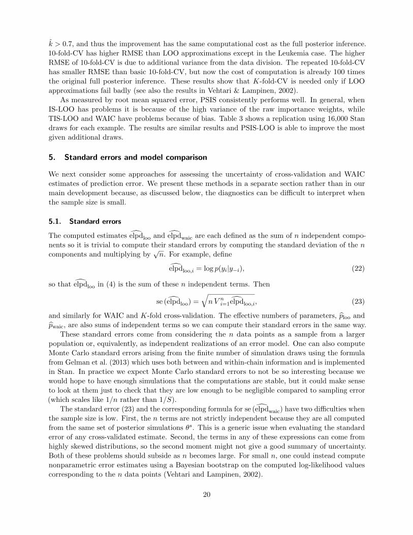
5. Standard errors and model comparison

We next consider some approaches for assessing the uncertainty of cross-validation and WAIC

estimates of prediction error. We present these methods in a separate section rather than in our

main development because, as discussed below, the diagnostics can be difficult to interpret when

the sample size is small.

5.1. Standard errors

The computed estimates elpdloo and elpdwaic are each defined as the sum of n independent compo-

nents so it is trivial to compute their standard errors by computing the standard deviation of the n

components and multiplying by√n. For example, define

elpdloo,i = log p(yi|y−i), (22)

so that elpdloo in (4) is the sum of these n independent terms. Then

se (elpdloo) =

√nV n

i=1elpdloo,i, (23)

and similarly for WAIC and K-fold cross-validation. The effective numbers of parameters, ploo and

pwaic, are also sums of independent terms so we can compute their standard errors in the same way.

These standard errors come from considering the n data points as a sample from a larger

population or, equivalently, as independent realizations of an error model. One can also compute

Monte Carlo standard errors arising from the finite number of simulation draws using the formula

from Gelman et al. (2013) which uses both between and within-chain information and is implemented

in Stan. In practice we expect Monte Carlo standard errors to not be so interesting because we

would hope to have enough simulations that the computations are stable, but it could make sense

to look at them just to check that they are low enough to be negligible compared to sampling error

(which scales like 1/n rather than 1/S).

The standard error (23) and the corresponding formula for se (elpdwaic) have two difficulties when

the sample size is low. First, the n terms are not strictly independent because they are all computed

from the same set of posterior simulations θs. This is a generic issue when evaluating the standard

error of any cross-validated estimate. Second, the terms in any of these expressions can come from

highly skewed distributions, so the second moment might not give a good summary of uncertainty.

Both of these problems should subside as n becomes large. For small n, one could instead compute

nonparametric error estimates using a Bayesian bootstrap on the computed log-likelihood values

corresponding to the n data points (Vehtari and Lampinen, 2002).

20

5.2. Model comparison

When comparing two fitted models, we can estimate the difference in their expected predictive

accuracy by the difference in elpdloo or elpdwaic (multiplied by −2, if desired, to be on the deviance

scale). To compute the standard error of this difference we can use a paired estimate to take

advantage of the fact that the same set of n data points is being used to fit both models.

For example, suppose we are comparing models A and B, with corresponding fit measures

elpdA

loo=∑n

i=1 elpdA

loo,i and elpdB

loo=∑n

i=1 elpdB

loo,i. The standard error of their difference is simply,

se (elpdA

loo − elpdB

loo) =

√nV n

i=1(elpdA

loo,i − elpdB

loo,i), (24)

and similarly for WAIC and K-fold cross-validation. Alternatively the non-parametric Bayesian

bootstrap approach can be used (Vehtari and Lampinen, 2002).

As before, these calculations should be most useful when n is large, because then non-normality

of the distribution is not such an issue when estimating the uncertainty of these sums.

In any case, we suspect that these standard error formulas, for all their flaws, should give a

better sense of uncertainty than what is obtained using the current standard approach for comparing

differences of deviances to a χ2 distribution, a practice that is derived for Gaussian linear models or

asymptotically and, in any case, only applies to nested models.

Further research needs to be done to evaluate the performance in model comparison of (24)

and the corresponding standard error formula for LOO. Cross-validation and WAIC should not be

used to select a single model among a large number of models due to a selection induced bias as

demonstrated, for example, by Piironen and Vehtari (2016).

We demonstrate the practical use of LOO in model comparison using the radon example from

Section 4.6. Model A is the multilevel linear model discussed in Section 4.6 and Model B is the same

model but without the county-level uranium predictor. That is, at the county-level Model B has

(αjβj

)∼ N

((µαµβ

),

(σ2α ρσασβ

ρσασβ σ2β

)), j = 1, . . . , 85.

Comparing the models on PSIS-LOO reveals an estimated difference in elpd of 10.2 (with a standard

error of 5.1) in favor of Model A.

5.3. Model comparison using pointwise prediction errors

We can also compare models in their leave-one-out errors, point by point. We illustrate with an

analysis of a survey of residents from a small area in Bangladesh that was affected by arsenic in

drinking water. Respondents with elevated arsenic levels in their wells were asked if they were

interested in getting water from a neighbor’s well, and a series of models were fit to predict this

binary response given various information about the households (Gelman and Hill, 2007).

Here we start with a logistic regression for the well-switching response given two predictors: the

arsenic level of the water in the resident’s home, and the distance of the house from the nearest

safe well. We compare this to an alternative logistic regression where the arsenic predictor on

the logarithmic scale. The two models have the same number of parameters but give different

predictions.

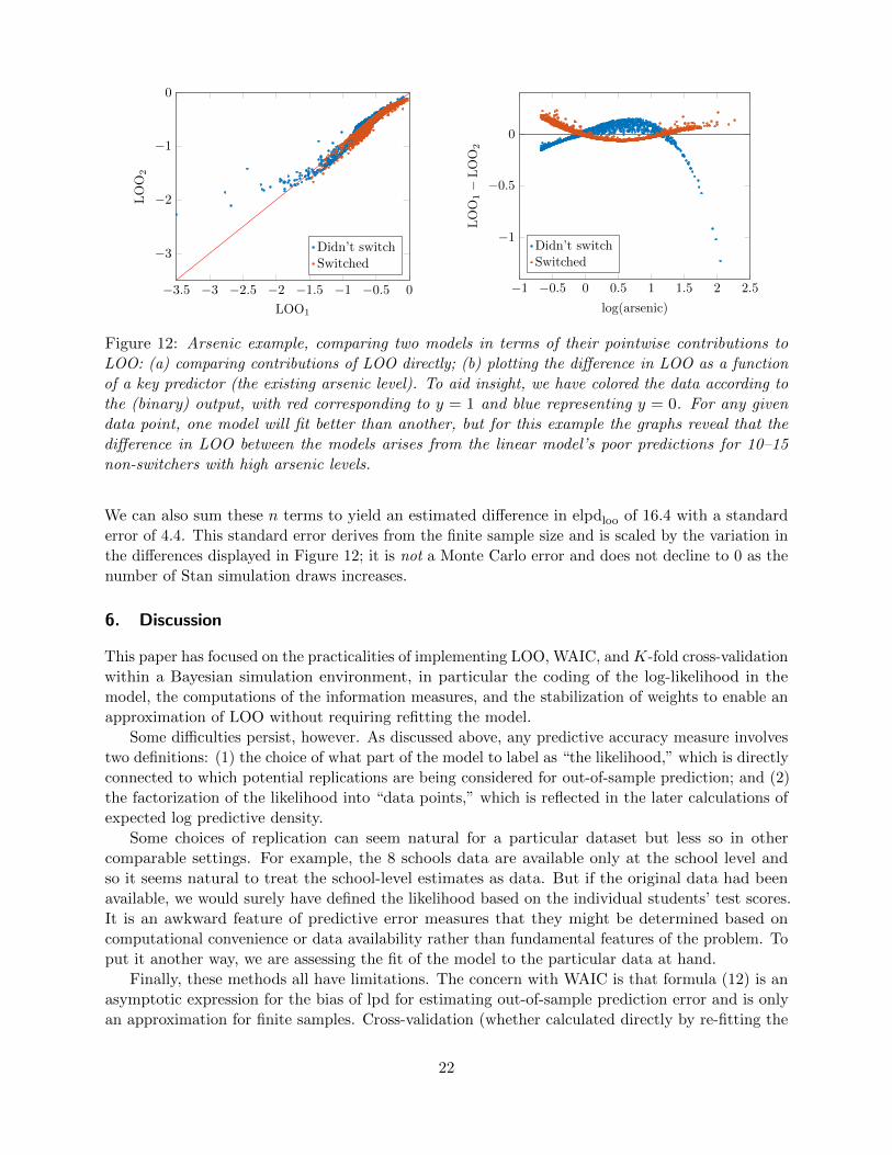
Figure 12 shows the pointwise results for the arsenic example. The scattered blue dots on the

left side of Figure 12a and on the lower right of Figure 12b correspond to data points which Model A

fits particularly poorly—that is, large negative contributions to the expected log predictive density.

21

−3.5 −3 −2.5 −2 −1.5 −1 −0.5 0

−3

−2

−1

0

LOO1

LOO

2

Didn’t switchSwitched

−1 −0.5 0 0.5 1 1.5 2 2.5

−1

−0.5

0

log(arsenic)

LOO

1−LOO

2

Didn’t switchSwitched

Figure 12: Arsenic example, comparing two models in terms of their pointwise contributions to

LOO: (a) comparing contributions of LOO directly; (b) plotting the difference in LOO as a function

of a key predictor (the existing arsenic level). To aid insight, we have colored the data according to

the (binary) output, with red corresponding to y = 1 and blue representing y = 0. For any given

data point, one model will fit better than another, but for this example the graphs reveal that the

difference in LOO between the models arises from the linear model’s poor predictions for 10–15

non-switchers with high arsenic levels.

We can also sum these n terms to yield an estimated difference in elpdloo of 16.4 with a standard

error of 4.4. This standard error derives from the finite sample size and is scaled by the variation in

the differences displayed in Figure 12; it is not a Monte Carlo error and does not decline to 0 as the

number of Stan simulation draws increases.

6. Discussion

This paper has focused on the practicalities of implementing LOO, WAIC, and K-fold cross-validation

within a Bayesian simulation environment, in particular the coding of the log-likelihood in the

model, the computations of the information measures, and the stabilization of weights to enable an

approximation of LOO without requiring refitting the model.

Some difficulties persist, however. As discussed above, any predictive accuracy measure involves

two definitions: (1) the choice of what part of the model to label as “the likelihood,” which is directly

connected to which potential replications are being considered for out-of-sample prediction; and (2)

the factorization of the likelihood into “data points,” which is reflected in the later calculations of

expected log predictive density.

Some choices of replication can seem natural for a particular dataset but less so in other

comparable settings. For example, the 8 schools data are available only at the school level and

so it seems natural to treat the school-level estimates as data. But if the original data had been

available, we would surely have defined the likelihood based on the individual students’ test scores.

It is an awkward feature of predictive error measures that they might be determined based on

computational convenience or data availability rather than fundamental features of the problem. To

put it another way, we are assessing the fit of the model to the particular data at hand.

Finally, these methods all have limitations. The concern with WAIC is that formula (12) is an

asymptotic expression for the bias of lpd for estimating out-of-sample prediction error and is only

an approximation for finite samples. Cross-validation (whether calculated directly by re-fitting the

22

model to several different data subsets, or approximated using importance sampling as we did for

LOO) has a different problem in that it relies on inference from a smaller subset of the data being

close to inference from the full dataset, an assumption that is typically but not always true.

For example, as we demonstrated in Section 4.1, in a hierarchical model with only one data point

per group, PSIS-LOO and WAIC can dramatically understate prediction accuracy. Another setting

where LOO (and cross-validation more generally) can fail is in models with weak priors and sparse

data. For example, consider logistic regression with flat priors on the coefficients and data that

happen to be so close to separation that the removal of a single data point can induce separation and

thus infinite parameter estimates. In this case the LOO estimate of average prediction accuracy will

be zero (that is, elpdis−loo will be −∞) if it is calculated to full precision, even though predictions

of future data from the actual fitted model will have bounded loss. Such problems should not arise

asymptotically with a fixed model and increasing sample size but can occur with actual finite data,

especially in settings where models are increasing in complexity and are insufficiently constrained.

That said, quick estimates of out-of-sample prediction error can be valuable for summarizing

and comparing models, as can be seen from the popularity of AIC and DIC. For Bayesian models,

we prefer PSIS-LOO and K-fold cross-validation to those approximations which are based on point

estimation.

References

Akaike, H. (1973). Information theory and an extension of the maximum likelihood principle. In

Proceedings of the Second International Symposium on Information Theory, ed. B. N. Petrov

and F. Csaki, 267–281. Budapest: Akademiai Kiado.

Ando, T., and Tsay, R. (2010). Predictive likelihood for Bayesian model selection and averaging.

International Journal of Forecasting 26, 744–763.

Arolot, S., and Celisse, A. (2010). A survey of cross-validation procedures for model selection.

Statistics Surveys 4, 40–79.

Burman, P. (1989). A comparative study of ordinary cross-validation, v-fold cross-validation and

the repeated learning-testing methods. Biometrika 76, 503–514.

Epifani, I., MacEachern, S. N., and Peruggia, M. (2008). Case-deletion importance sampling

estimators: Central limit theorems and related results. Electronic Journal of Statistics 2,

774–806.

Gabry, J., and Goodrich, B. (2016). rstanarm: Bayesian applied regression modeling via Stan. R

package version 2.10.0. http://mc-stan.org/interfaces/rstanarm

Geisser, S., and Eddy, W. (1979). A predictive approach to model selection. Journal of the American

Statistical Association 74, 153–160.

Gelfand, A. E. (1996). Model determination using sampling-based methods. In Markov Chain

Monte Carlo in Practice, ed. W. R. Gilks, S. Richardson, D. J. Spiegelhalter, 145–162. London:

Chapman and Hall.

Gelfand, A. E., Dey, D. K., and Chang, H. (1992). Model determination using predictive distributions

with implementation via sampling-based methods. In Bayesian Statistics 4, ed. J. M. Bernardo,

J. O. Berger, A. P. Dawid, and A. F. M. Smith, 147–167. Oxford University Press.

Gelman, A., Carlin, J. B., Stern, H. S., Dunson, D. B., Vehtari, A., and Rubin D. B. (2013).

Bayesian Data Analysis, third edition. London: CRC Press.

23

Gelman, A., and Hill, J. (2007). Data Analysis Using Regression and Multilevel/Hierarchical Models.

Cambridge University Press.

Gelman, A., Hwang, J., and Vehtari, A. (2014). Understanding predictive information criteria for

Bayesian models. Statistics and Computing 24, 997–1016.

Hoeting, J., Madigan, D., Raftery, A. E., and Volinsky, C. (1999). Bayesian model averaging.

Statistical Science 14, 382–417.

Hoffman, M. D., and Gelman, A. (2014). The no-U-turn sampler: Adaptively setting path lengths

in Hamiltonian Monte Carlo. Journal of Machine Learning Research 15, 15931623.

Ionides, E. L. (2008). Truncated importance sampling. Journal of Computational and Graphical

Statistics 17, 295-311.

Kong, A., Liu, J. S., and Wong, W. H. (1994). Sequential imputations and Bayesian missing data

problems. Journal of the American Statistical Association 89, 278–288.

Koopman, S. J., Shephard, N., and Creal, D. (2009). Testing the assumptions behind importance

sampling. Journal of Econometrics 149, 2–11.

Peruggia, M. (1997). On the variability of case-deletion importance sampling weights in the Bayesian

linear model. Journal of the American Statistical Association 92, 199–207.

Piironen, J., and Vehtari, A. (2016). Comparison of Bayesian predictive methods for model

selection. Statistics and Computing. In press. http://link.springer.com/article/10.1007/

s11222-016-9649-y

Plummer, M. (2008). Penalized loss functions for Bayesian model comparison. Biostatistics 9,

523–539.

R Core Team (2016). R: A language and environment for statistical computing. R Foundation for

Statistical Computing, Vienna, Austria. https://www.R-project.org/

Rubin, D. B. (1981). Estimation in parallel randomized experiments. Journal of Educational

Statistics 6, 377–401.

Spiegelhalter, D. J., Best, N. G., Carlin, B. P., and van der Linde, A. (2002). Bayesian measures of

model complexity and fit. Journal of the Royal Statistical Society B 64, 583–639.

Spiegelhalter, D., Thomas, A., Best, N., Gilks, W., and Lunn, D. (1994, 2003). BUGS: Bayesian

inference using Gibbs sampling. MRC Biostatistics Unit, Cambridge, England.

http://www.mrc-bsu.cam.ac.uk/bugs/

Stan Development Team (2016a). The Stan C++ Library, version 2.10.0. http://mc-stan.org/

Stan Development Team (2016b). RStan: the R interface to Stan, version 2.10.1.

http://mc-stan.org/interfaces/rstan.html

Stone, M. (1977). An asymptotic equivalence of choice of model cross-validation and Akaike’s

criterion. Journal of the Royal Statistical Society B 36, 44–47.

van der Linde, A. (2005). DIC in variable selection. Statistica Neerlandica 1, 45–56.

Vehtari, A., and Gelman, A. (2015). Pareto smoothed importance sampling. arXiv:1507.02646.

Vehtari, A., Gelman, A., and Gabry, J. (2016). loo: Efficient leave-one-out cross-validation and

WAIC for Bayesian models. R package version 0.1.6. https://github.com/stan-dev/loo

Vehtari, A., Mononen, T., Tolvanen, V., Sivula, T., and Winther, O. (2016). Bayesian leave-one-

out cross-validation approximations for Gaussian latent variable models. Journal of Machine

Learning Research, accepted for publication. arXiv preprint arXiv:1412.7461.

Vehtari, A., and Lampinen, J. (2002). Bayesian model assessment and comparison using cross-

validation predictive densities. Neural Computation 14, 2439–2468.

24

Vehtari, A., and Ojanen, J. (2012). A survey of Bayesian predictive methods for model assessment,

selection and comparison. Statistics Surveys 6, 142–228.

Vehtari, A., and Riihimaki, J. (2014). Laplace approximation for logistic Gaussian process density

estimation and regression. Bayesian analysis, 9, 425-448.

Watanabe, S. (2010). Asymptotic equivalence of Bayes cross validation and widely applicable

information criterion in singular learning theory. Journal of Machine Learning Research 11,

3571–3594.

Zhang, J., and Stephens, M. A. (2009). A new and efficient estimation method for the generalized

Pareto distribution. Technometrics 51, 316–325.

A. Implementation in Stan and R

A.1. Stan code for computing and storing the pointwise log-likelihood

We illustrate how to write Stan code that computes and stores the pointwise log-likelihood using

the arsenic example from Section 5.3. We save the program in the file logistic.stan:

data {

int N;

int P;

int<lower=0,upper=1> y[N];

matrix[N,P] X;

}

parameters {

vector[P] b;

}

model {

b ~ normal(0,1);

y ~ bernoulli_logit(X*b);

}

generated quantities {

vector[N] log_lik;

for (n in 1:N)

log_lik[n] = bernoulli_logit_lpmf(y[n] | X[n]*b);

}

We have defined the log-likelihood as a vector log lik in the generated quantities block so that

the individual terms will be saved by Stan.6 It would seem desirable to compute the terms of the

log-likelihood directly without requiring the repetition of code, perhaps by flagging the appropriate

lines in the model or by identifying the log likelihood as those lines in the model that are defined

relative to the data. But there are so many ways of writing any model in Stan—anything goes as

long as it produces the correct log posterior density, up to any arbitrary constant—that we cannot

see any general way at this time for computing LOO and WAIC without repeating the likelihood

part of the code. The good news is that the additional computations are relatively cheap: sitting as

they do in the generated quantities block (rather than in the transformed parameters and model

blocks), the expressions for the terms of the log posterior need only be computed once per saved

iteration rather than once per HMC leapfrog step, and no gradient calculations are required.

6 The code in the generated quantities block is written using the new syntax introduced in Stan version 2.10.0.

25

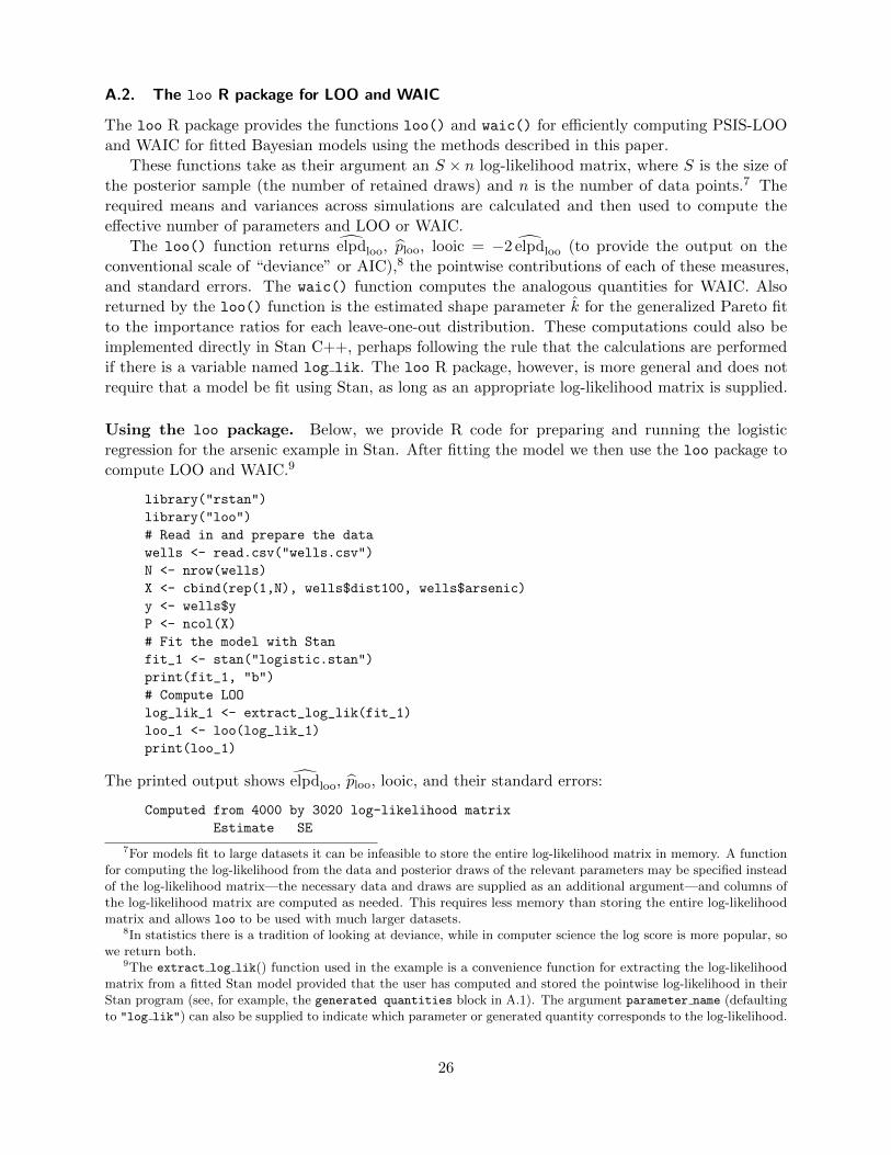
A.2. The loo R package for LOO and WAIC

The loo R package provides the functions loo() and waic() for efficiently computing PSIS-LOO

and WAIC for fitted Bayesian models using the methods described in this paper.

These functions take as their argument an S × n log-likelihood matrix, where S is the size of

the posterior sample (the number of retained draws) and n is the number of data points.7 The

required means and variances across simulations are calculated and then used to compute the

effective number of parameters and LOO or WAIC.

The loo() function returns elpdloo, ploo, looic = −2 elpdloo (to provide the output on the

conventional scale of “deviance” or AIC),8 the pointwise contributions of each of these measures,

and standard errors. The waic() function computes the analogous quantities for WAIC. Also

returned by the loo() function is the estimated shape parameter k for the generalized Pareto fit

to the importance ratios for each leave-one-out distribution. These computations could also be

implemented directly in Stan C++, perhaps following the rule that the calculations are performed

if there is a variable named log lik. The loo R package, however, is more general and does not

require that a model be fit using Stan, as long as an appropriate log-likelihood matrix is supplied.

Using the loo package. Below, we provide R code for preparing and running the logistic

regression for the arsenic example in Stan. After fitting the model we then use the loo package to

compute LOO and WAIC.9

library("rstan")

library("loo")

# Read in and prepare the data

wells <- read.csv("wells.csv")

N <- nrow(wells)

X <- cbind(rep(1,N), wells$dist100, wells$arsenic)

y <- wells$y

P <- ncol(X)

# Fit the model with Stan

fit_1 <- stan("logistic.stan")

print(fit_1, "b")

# Compute LOO

log_lik_1 <- extract_log_lik(fit_1)

loo_1 <- loo(log_lik_1)

print(loo_1)

The printed output shows elpdloo, ploo, looic, and their standard errors:

Computed from 4000 by 3020 log-likelihood matrix

Estimate SE

7For models fit to large datasets it can be infeasible to store the entire log-likelihood matrix in memory. A functionfor computing the log-likelihood from the data and posterior draws of the relevant parameters may be specified insteadof the log-likelihood matrix—the necessary data and draws are supplied as an additional argument—and columns ofthe log-likelihood matrix are computed as needed. This requires less memory than storing the entire log-likelihoodmatrix and allows loo to be used with much larger datasets.

8In statistics there is a tradition of looking at deviance, while in computer science the log score is more popular, sowe return both.

9The extract log lik() function used in the example is a convenience function for extracting the log-likelihoodmatrix from a fitted Stan model provided that the user has computed and stored the pointwise log-likelihood in theirStan program (see, for example, the generated quantities block in A.1). The argument parameter name (defaultingto "log lik") can also be supplied to indicate which parameter or generated quantity corresponds to the log-likelihood.

26

elpd_loo -1968.3 15.6

p_loo 3.1 0.1

looic 3936.6 31.2

All Pareto k estimates OK (k < 0.5)

By default, the estimates for the shape parameter k of the generalized Pareto distribution

are also checked and a message is displayed informing the user if any k are problematic (see the

end of Section 2.1). In the example above the message tells us that all of the estimates for k are

fine. However, if any k were between 1/2 and 1 or greater than 1 the message would instead look

something like this:

Warning messages:

1: 200 (7%) Pareto k estimates between 0.5 and 1

2: 85 (3%) Pareto k estimates greater than 1

If there are any warnings then it can be useful to visualize the estimates to check which data points

correspond to the large k values. A plot of the k estimates can also be generated using plot(loo1)

and the list returned by the loo function also contains the full vector of k values.

Model comparison. To compare this model to a second model on their values of LOO we can

use the compare function:

# First fit a second model, using log(arsenic) instead of arsenic

X <- cbind(rep(1,N), wells$dist100, log(wells$arsenic))

P <- ncol(X)

fit_2 <- stan("logistic.stan")

print(fit_2, "b")

log_lik_2 <- extract_log_lik(fit_2)

loo_2 <- loo(log_lik_2)

# Compare the models

loo_diff <- compare(loo_1, loo_2)

print(loo_diff)

This new object, loo diff, contains the estimated difference of expected leave-one-out prediction

errors between the two models, along with the standard error:

elpd_diff SE

16.1 4.4

Code for WAIC. For WAIC the code is analogous and the objects returned have the same

structure (except there are no Pareto k estimates). The compare() function can also be used to

estimate the difference in WAIC between two models:

waic_1 <- waic(log_lik_1)

waic_2 <- waic(log_lik_2)

waic_diff <- compare(waic_1, waic_2)

27

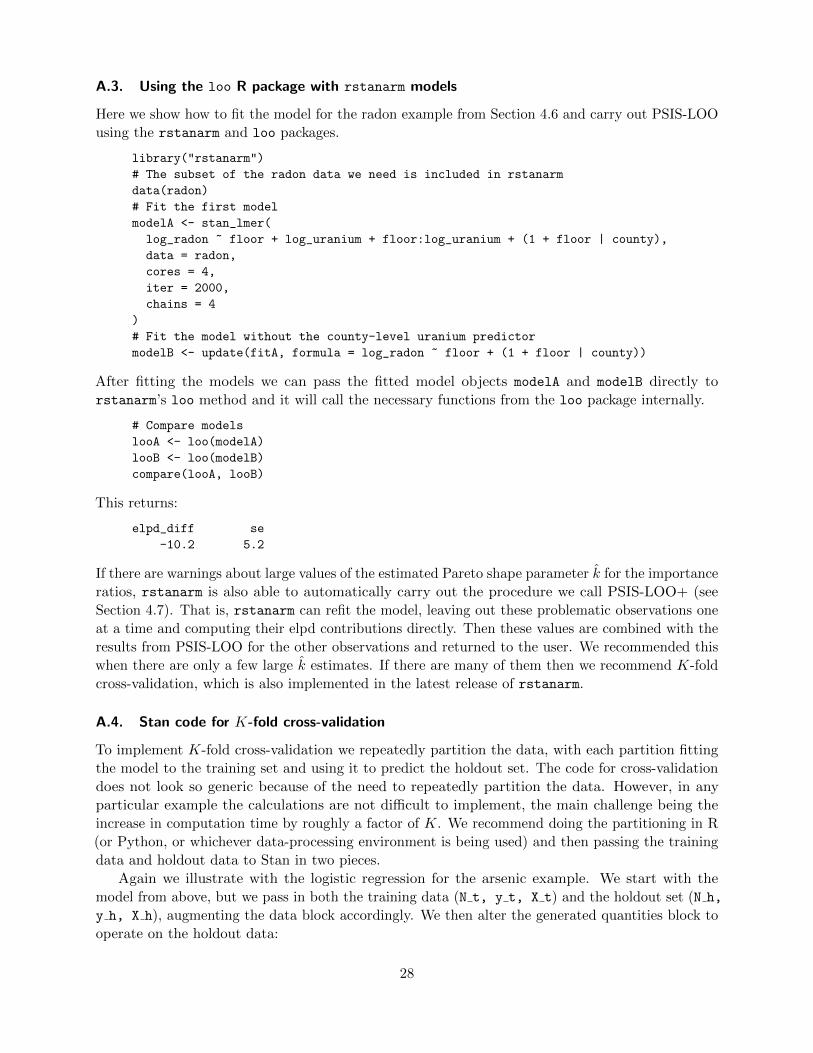
A.3. Using the loo R package with rstanarm models

Here we show how to fit the model for the radon example from Section 4.6 and carry out PSIS-LOO

using the rstanarm and loo packages.

library("rstanarm")

# The subset of the radon data we need is included in rstanarm

data(radon)

# Fit the first model

modelA <- stan_lmer(

log_radon ~ floor + log_uranium + floor:log_uranium + (1 + floor | county),

data = radon,

cores = 4,

iter = 2000,

chains = 4

)

# Fit the model without the county-level uranium predictor

modelB <- update(fitA, formula = log_radon ~ floor + (1 + floor | county))

After fitting the models we can pass the fitted model objects modelA and modelB directly to

rstanarm’s loo method and it will call the necessary functions from the loo package internally.

# Compare models

looA <- loo(modelA)

looB <- loo(modelB)

compare(looA, looB)

This returns:

elpd_diff se

-10.2 5.2

If there are warnings about large values of the estimated Pareto shape parameter k for the importance

ratios, rstanarm is also able to automatically carry out the procedure we call PSIS-LOO+ (see

Section 4.7). That is, rstanarm can refit the model, leaving out these problematic observations one

at a time and computing their elpd contributions directly. Then these values are combined with the

results from PSIS-LOO for the other observations and returned to the user. We recommended this

when there are only a few large k estimates. If there are many of them then we recommend K-fold

cross-validation, which is also implemented in the latest release of rstanarm.

A.4. Stan code for K-fold cross-validation

To implement K-fold cross-validation we repeatedly partition the data, with each partition fitting

the model to the training set and using it to predict the holdout set. The code for cross-validation

does not look so generic because of the need to repeatedly partition the data. However, in any

particular example the calculations are not difficult to implement, the main challenge being the

increase in computation time by roughly a factor of K. We recommend doing the partitioning in R

(or Python, or whichever data-processing environment is being used) and then passing the training

data and holdout data to Stan in two pieces.

Again we illustrate with the logistic regression for the arsenic example. We start with the

model from above, but we pass in both the training data (N t, y t, X t) and the holdout set (N h,

y h, X h), augmenting the data block accordingly. We then alter the generated quantities block to

operate on the holdout data:

28

data {

int P; // Number of regression predictors

int N_t; // (Training) number of data points

int<lower=0,upper=1> y_t[N_t]; // (Training) binary data

matrix[N_t,P] X_t; // (Training) predictors

int N_h; // (Holdout)

int y_h[N_h]; // (Holdout)

matrix[N_h,P] X_h; // (Holdout)

real a;

}

parameters {

vector[P] b;

}

model {

y_t ~ bernoulli_logit(X_t*b);

}

generated quantities {

vector[N_t] log_lik_t;

vector[N_h] log_lik_h;

for (n in 1:N_t)

log_lik_t[n] = bernoulli_logit_lpmf(y_t[n] | X_t[n]*b);

for (n in 1:N_h)

log_lik_h[n] = bernoulli_logit_lpmf(y_h[n] | X_h[n]*b);

}

LOO could be also implemented in this way, setting Nt to N − 1 and Nh to 1. But, as discussed in

the article, for large datasets it is more practical to approximate LOO using importance sampling

on the draws from the posterior distribution fit to the entire dataset.

29