practical application and empirical evaluation of reference class forecasting...

36 October/November 2016 ■ Project Management Journal

PA

PE

RS

IntroductIon

Before a project is started, project managers have to make an estimation of how long the project will take and how much it is going to cost. Traditionally, project managers focus on the specifics of the considered project (e.g., its particular activities) to produce these

estimations, as they attempt to forecast uncertain events that would influence the future course of the project. Such an “inside view” forecasting approach is obviously based on human judgment. In their studies, Kahneman and Tversky (1979a, 1979b) found that human judgment is biased, as it is generally too optimistic because of overconfidence and insufficient regard to actual previous experience (i.e., “optimism bias”). Moreover, project managers could deliberately and strategically underestimate costs (and durations) to give the impression that they would surpass the competition (i.e., “strategic misinterpretation”). In order to overcome this human bias and the inaccurate forecasts that result from it, Kahneman and Tversky (1979a) and later Lovallo and Kahneman (2003) introduced the method of reference class forecasting (RCF). RCF takes an “outside view” on planned actions rather than an inside view by cutting directly to outcomes through the use of distributional information from other projects similar to the one being forecasted. More specifically, the RCF method consists of a three-step procedure (Flyvbjerg, 2006, 2007):

1. Identifying a relevant reference class of past projects similar to the considered project

2. Establishing a probability distribution for the selected reference class3. Determining the most likely outcome for the considered project by

comparing that project with the reference class distribution

Regarding the first step, Flyvbjerg (2006) states that the reference class must be broad enough to be meaningful, but narrow enough to be truly comparable with the considered project. We will approach this statement from a quanti-tative point of view by identifying reference classes with different degrees of similarity and evaluating their performance, which has not been done in earlier studies.

Notice that the RCF method, as described by the three-step proce-dure, does not involve any attempt to forecast specific events that would affect the particular project. Multiple experimental studies (Kahneman, 1994; Kahneman & Tversky, 1979a, 1979b; Lovallo & Kahneman, 2003)

Practical Application and Empirical Evaluation of Reference Class Forecasting for Project ManagementJordy Batselier, Faculty of Economics and Business Administration, Ghent University, Ghent, BelgiumMario Vanhoucke, Ghent University and Vlerick Business School, Ghent, Belgium; UCL School of Management, University College London, London, United Kingdom

Traditionally, project managers produce

cost and time forecasts by predicting the

future course of specific events. In contrast,

reference class forecasting (RCF) bypasses

human judgment by basing forecasts on the

actual outcomes of past projects similar to

the project being forecasted. The RCF tech-

nique is compared with the most common

traditional project forecasting methods, such

as those based on Monte Carlo simulation

and earned value management (EVM). The

conducted evaluation is entirely based on

real-life project data and shows that RCF

indeed performs best, for both cost and time

forecasting, and therefore supports the prac-

tical relevance of the technique.

KEYWORDS: project management;

project forecasting; reference class

forecasting; earned value management;

Monte Carlo simulation; empirical database

Project Management Journal, Vol. 47, No. 5, 36–51

© 2016 by the Project Management Institute

Published online at www.pmi.org/PMJ

ABStrAct ■

101278_PMJ_03_036-051.indd 36 9/7/16 10:26 PM

October/November 2016 ■ Project Management Journal 37

• Identify other realistic causes for biased forecasts that occur in practice, different from the traditional defini-tions of optimism bias and strategic misinterpretation; and

• Further support the practical relevance of the RCF technique for real-life applications.

Regarding the first objective, the forecasts used for comparison are those from EVM, Monte Carlo simulation, and baseline estimates. Note that the two latter forecasts have not been explicitly considered in the study of Batselier and Vanhoucke (2015b). In order to achieve the last two objectives, we base our study on a real-life construction project that originates from the empirical proj-ect database of Batselier and Vanhoucke (2015a). Furthermore, all projects of the different reference classes are also part of this database. Given the extent of the employed data, it is not our goal to pursue generalizability. Rather, we aim at providing a clear view of the practical application of different project forecast-ing methods—in particular, RCF—and obtaining a reliable indication of the relevance of RCF in terms of workability and performance with respect to the traditional forecasting methods.

More information about the con-sidered project and the real-life project database is provided in the next section, followed by the presentation of the dif-ferent project forecasting methods con-sidered in this article. In a subsequent section, the results of these methods are compared and discussed. Conclu-sively, the most important outcomes of our study are summarized and sugges-tions for future research are made.

MethodologyWe will start this section with the pre-sentation of the real-life construction project that forms the basis for the cur-rent study. Then the empirical database from which the considered project orig-inates is described. Moreover, the refer-ence classes that are selected in this study all consist of projects that are part

and PD represent the baseline schedule (BLS) of the project (i.e., the planned course of the project) and are, there-fore, collectively termed baseline esti-mates here. The baseline estimates are used as inputs for the earned value man-agement (EVM) methodology. EVM is a widely accepted technique for perform-ing project control that integrates the three critical project management ele-ments of cost, schedule, and scope. The technique also implicitly incorporates the quality aspect by taking into account project progress (Willems & Vanhoucke, 2015). Through the application of EVM, the project manager can monitor the performance of the project during exe-cution and receive warning signals for taking corrective actions needed to get the project back on track. Furthermore, the EVM technique can also be used to produce project forecasts. However, because EVM is a technique for perform-ing project control, the forecasts are pro-duced at different tracking periods (TPs) (i.e., evaluation moments) during the project’s progress. RCF-based forecasts, on the other hand, are made before the project starts. Nevertheless, the pre-project forecasts from RCF and the inter-mediately revised forecasts from EVM will be compared. In this light, RCF is seen as a technique for obtaining constant— and, therefore, stable—project forecasts, like the method proposed by Warburton (2011). The results of the RCF method will also be compared with the forecasts obtained from a pre-project Monte Carlo (MC) simulation, the specifics of which will be presented in the next section.

To provide a clear overview of the con-tributions of this article, we now explicitly summarize the intended objectives:

• Perform a quantitative evaluation of the RCF technique by comparing it with the most common traditional project forecasting methods;

• Apply RCF for project duration forecast-ing and evaluating the performance;

• Assess the influence of different selec-tions of reference classes with respect to similarity levels;

have indicated that RCF is more accu-rate than traditional forecasting meth-ods. However, these studies were not situated in the field of project manage-ment. The first and only instance of RCF in project management was presented by Flyvbjerg (2006), who considered a project in the transportation sector, though no quantitative evaluation of the accuracy of the RCF technique was per-formed. Therefore, this article will com-pare the performance of RCF with that of the most common traditional meth-ods for project forecasting. Moreover, this performance evaluation is not based solely on the most important forecasting quality criterion, accuracy (Carbone & Armstrong, 1982), but also on the two other criteria—timeliness and stability (Covach, Haydon, & Reither, 1981)—the latter not being considered by Batselier and Vanhoucke (2015b). Furthermore, and in contrast to Flyvbjerg’s (2006) study, RCF will not only be applied for forecasting project cost but also for proj-ect duration. As might appear from the above discussion, the focus of this article is on the time and cost aspects of project management. Although these are per-haps the two most important objectives for the project manager, other factors such as safety, sustainability, and espe-cially quality are also of interest. How-ever, it is outside the scope of this article to further elaborate on the latter factors. An overview of studies that incorporate quality, safety, and/or sustainability in the traditional time–cost project control framework is provided by Willems and Vanhoucke (2015). Nevertheless, the expansion of control models through the integration of other performance-defining factors, in addition to time and cost, remains a research path that should receive more attention in the future.

RCF produces forecasts prior to the project start. This corresponds to the budget at completion (BAC) and planned duration (PD) that reflect the final cost and duration of the project, respectively, estimated by the project managers based on their expectations of the future course of the project (i.e., inside view). The BAC

101278_PMJ_03_036-051.indd 37 9/7/16 10:26 PM

Practical Application and Empirical Evaluation of Reference Class Forecasting


PA

PE

RS

of the said database. After the selec-tion of the different reference classes, the RCF method will be applied. Sub-sequently, we present the traditional project forecasting approaches that are considered for comparison: first, those that produce pre-project forecasts, and then those that yield forecasts during project execution. More concretely, the consecutive subsections will be about baseline estimates, Monte Carlo simu-lation, and EVM, respectively. For each forecasting method, both cost and time forecasting are considered.

Project Description

The study in this article is based on a real-life construction project. More specifically, it concerns the execution of the finishing works inside an office building, comprising the interior join-ery and the placement of plaster walls, movable partition walls (also acoustic), raised floors, suspended ceilings, and furniture. The works are performed by a medium-sized finishing construction company with extensive experience in the field. Nevertheless, the consid-ered project comprises a few smaller activities that are rather uncommon for the company, such as the placement of carpets and special glass walls. The complete list of activities, together with their planned costs and durations (i.e., the BLS), is shown in Table 1. Note that the last column of this table contains information that will be considered and discussed later in this article.

The outwardly irregular activity IDs (identification numbers) were chosen by the project manager who was respon-sible for this project and are therefore retained here. Durations are expressed in standard eight-hour working days. The displayed costs and durations rep-resent the pre-project expectations of the project manager.

The precedence relations between the activities—which express techni-cal constraints—are also displayed in Table 1. When there are no parentheses behind the listed activity IDs, the pre-cedence relation is a finish-start (FS)

ID Activity Name Predecessors SuccessorsCost [€]

Duration [d]

Distr Prof

1 Fixed ceilings 4(SS);6(SS);17 2,129 89 symm

2 Metal ceilings 4(SS);6(SS);17 19,509 89 symm

4 Movable partition walls (1)

1(SS);2(SS) 37,641 151 right

6 Plaster walls 1(SS);2(SS) 9(FF);10 36,184 22 left

9 Full subcontracting (1) 6(FF) 1,079 1 no risk

10 Disassembling ceilings 6 12 2,509 7 symm

12 Adjusting raised floor 10 11;21;3 1,800 3 symm

11 Placing carpet 12 13 27,162 5 symm

21 Full subcontracting (2) 12 20,068 67 no risk

13 Placing furniture 11 14;16 36,023 3 symm

14 Placing glass walls 13 17 180 1 symm

3 Acoustic dams 12 20;5;7;8 1,674 2 left


3 17;15;22 4,926 9 right


3 17;15;22 619 9 right

7 Doors 3 17;15;22 6,259 3 symm

8 Joinery 3 17;15;22 1,964 3 symm

17 Painting works 1;2;14;20;5;7;8 19(SS) 8,538 41 symm

19 Ancillary works 17(SS) 16,619 3 symm

15 Finishings 20;5;7;8 18(SS) 13,132 71 symm

22 Miscellaneous 20;5;7;8 998 77 right

16 Adjusting furniture 13 312 61 symm

18 Moving reinforcing screens

15(SS) 4,879 3 symm

23 Additional work 0 0 no risk

Table 1: Activity information for the considered real-life construction project.

relation. An FS relation is the most com-mon type of precedence relation and indicates that an activity can only start after its predecessor(s) has (have) fin-ished. Start-start (SS) and finish-finish (FF) relations, on the other hand, signify that an activity can only start after its predecessor(s) has (have) started and that an activity can only finish after its predecessor(s) has (have) finished, respectively. The precedence relations between the activities can also be iden-tified from the Gantt chart in Figure 1.

Notice that, although all prece-dence relations have a zero time lag, the

activities almost never directly follow one another in the BLS. This indicates that the project manager has incorpo-rated buffers for activity durations in the project planning.

More extensive data on the con-sidered project can be found at www .or-as.be/research/database, because the project is part of the real-life project database of Batselier and Vanhoucke (2015a). In this database, which will be described in the following section, the considered project is identified by the code C2013-17 and the name Office Finishing Works (5).

101278_PMJ_03_036-051.indd 38 9/7/16 10:26 PM


sector is very broad, consisting of the civil, industrial, and building subsec-tors. The building construction subsec-tor, in turn, can be further subdivided into commercial, institutional, and residential building. Because the con-sidered project comprises the finishing works for an office building, it can be situated within the commercial building construction sector. Thus, three broader reference classes can be identified: projects from construction, building construction, and commercial build-ing construction, in order of increasing specificity and similarity to the consid-ered project. Projects from all of these (sub)sectors can be extracted from the database of Batselier and Vanhoucke (2015a). Logically, the broader the sector, the larger the number of rel-evant projects; this is also illustrated in Table 2, which shows the project codes and names of the projects within the dif-ferent reference classes. A number in a column indicates that the project in this study is part of the corresponding refer-ence class (Constr is construction, Build is building construction, and Comm is commercial building construction) for cost and/or time forecasting (C-column and T-column, respectively). Observe that there are four projects that can be

originate from the presented empirical database. How these different reference classes are composed is described in the next section.

Reference Class Selection

In order to apply the RCF technique, a reference class of projects similar to the considered project has to be iden-tified. As mentioned in the introduc-tion, it is our objective to assess the influence of the chosen reference class similarity level on the performance of RCF. To this end, we consider four different reference class composi-tions, ranging from broad sector-based to company-specific. Notice that this approach somewhat resembles the k-nearest neighbors (k-NN) nonpara-metric method, in which forecasts are based on the k projects closest (i.e., most similar) to the considered project. Paral-leling our approach, the fixed number k would thus be decreased to reflect the increasing similarity level of the refer-ence class. The explicit implementation of the k-NN method is beyond the scope of this article, but can be considered a potential future research topic.

Recall that the project considered in this study is a construction project. Note, however, that the construction

Database Description

The real-life project database utilized in this article was constructed by Batselier and Vanhoucke (2015a). At the time of this study, the ever-expanding database consisted of 56 projects, which originate from many different companies from various sectors (mainly construction, but also event management, IT, produc-tion, education, etc.) and show wide ranges of project budgets and dura-tions. The quality and authenticity of the project data are guaranteed by the application of a construction and eval-uation framework based on so-called project cards, which summarize the most important properties of a certain project and enable its categorization and evaluation (Batselier & Vanhoucke, 2015a). The project card of the project considered here—and of every other project in the database—is available at www.or-as.be/research/database, as are the project data themselves. The data were originally formatted as files from the project management software tool ProTrack (www.protrack.be), but can now also be obtained in Microsoft Excel format, thanks to the novel soft-ware tool PMConverter. Furthermore, all projects that constitute the refer-ence classes for the considered project

Figure 1: Gantt chart for the considered real-life construction project.

1246910121121131432057817191522161823

101278_PMJ_03_036-051.indd 39 9/7/16 10:26 PM



PA

PE

RS

In order to assess the influence of the reference class similarity level on the performance of the RCF tech-nique, all four of the reference classes included in Table 2 will be considered. The resulting cost and time forecasts are presented in the following section.

Reference Class Forecasting

In terms of the three-step procedure for applying RCF presented in the introduc-tion, we already performed the first step in the previous section (i.e., identify-ing relevant reference classes of past,

projects are available in the utilized database. All of them consist of activities that are strongly similar to those of the considered project, with the placement of the movable partition walls as the core activity. Moreover, the four projects were all completed in 2011, in the order indicated by the project codes (C2013-13 to 16) and names (Office Finishing Works [1] to [4]). The considered proj-ect C2013-17 Office Finishing Works (5) only started in May 2012, so the OFW reference class for this project is indeed constituted of past projects.

used in a reference class for time but not for cost forecasting. This is because authentic actual cost data for these proj-ects are absent. The numbers displayed in Table 2 will be explained and utilized in the next section.

The last two columns of Table 2 pres-ent the reference class “OFW” or “office finishing works.” This is the most specific reference class with the highest degree of similarity, as it only comprises the finishing construction projects executed by the same company as the one that did the considered project. Four of these

Reference Class

Constr Build Comm OFW

Code Name C [%] T [%] C [%] T [%] C [%] T [%] C [%] T [%]C2013-13 Office Finishing Works (1) 214.5 28.1 214.5 28.1 214.5 28.1 214.5 28.1

C2013-14 Office Finishing Works (2) 212.1 23.8 212.1 23.8 212.1 23.8 212.1 23.8



C2011-12 Claeys-Verhelst Premises — 2.7 — 2.7 — 2.7

C2013-09 Urban Development Project 10.4 23.7 10.4 23.7 10.4 23.7

C2013-03 Brussels Finance Tower 5.8 0.2 5.8 0.2

C2013-04 Kitchen Tower Anderlecht 18.9 36.0 18.9 36.0

C2013-06 Government Office Building 10.9 22.3 10.9 22.3

C2013-07 Family Residence 23.0 7.6 23.0 7.6

C2013-08 Timber House 15.1 8.8 15.1 8.8

C2013-12 Young Cattle Barn 7.5 63.5 7.5 63.5

C2014-01 Mixed-use Building 2.8 25.5 2.8 25.5

C2014-05 Apartment Building (1) — 20.2 — 20.2



C2014-08 Apartment Building (4) 19.5 18.0 19.5 18.0

C2011-13 Wind Farm 22.0 14.3

C2012-13 Pumping Station Jabbeke 4.2 12.0

C2013-01 Wiedauwkaai Fenders 22.9 0.0

C2013-02 Sewage Plant Hove 27.3 0.0

C2013-10 Town Square 33.2 20.1

C2013-11 Recreation Complex 20.5 211.4

C2014-04 Compressor Station Zelzate 5.0 62.5

Avg [%] 5.6 9.5 2.4 8.9 29.2 23.5 214.1 211.8

# projects 20 24 13 17 5 6 4 4

Table 2: Reference class selections and deviations between planned and actual outcomes.

101278_PMJ_03_036-051.indd 40 9/7/16 10:26 PM


profiles for the individual activity dura-tions. In this study, we apply triangular distribution profiles, which can be sym-metrical, skewed to the left, or skewed to the right. These profiles have predefined shapes (see Figure 2), as also used in earlier research (Batselier & Vanhoucke, 2015b). Furthermore, there is also the possibility that an activity exhibits no risk of its duration deviating from the expected value. The distribution profile in such a case is rather obvious (i.e., one single peak) and is therefore not included in Figure 2.

The worst case/best case duration of an activity is always 20% larger/smaller than its expected duration, regardless of the specific distribution profile (risk-free profile disregarded). Moreover, the expected duration of an activity corre-sponds to the 100% duration in Figure 2 and represents the duration estimated by the project management prior to the project start. These expected (or planned) activity duration values were already presented in the second to last column of Table 1. Notice that, for an activity with a distribution profile that is skewed to the left, there is a greater chance that the activity will take longer than expected, whereas the opposite is true for an activity with a right skewed distribution profile. It is important to realize that the assignment of distribu-tion profiles to the different activities of the considered project was performed by the project manager on the project based on his experiences from earlier projects that showed similar activities. Because historical data are used for this process, one would be inclined to regard

US$323,059) and the PD 161 days. The BAC can quite easily be calculated as the sum of all the activity costs displayed in Table 1. The calculation of the PD, on the other hand, is not as straightfor-ward, because the precedence relations between the different activities have to be respected. Only the activities that are part of the critical path (CP) define the PD. The critical activities of the consid-ered project are indicated by a different shade of gray in Figure 1. In fact, only the very long activity 4 is intrinsically critical, but activities 17, 22, and 16 also become critical because of the as late as possible (ALAP) planning approach adopted by the project management in question. Also note that the start of activity 4 is only planned after 10 days, whereas there is no technical constraint (i.e., precedence relation) that would inhibit the activity from beginning at project launch. The choice for delaying the start of activity 4—and for introduc-ing all other buffers in the project—was made by the project manager, perhaps taking into account the unavailability of a particular team or subcontractor until a certain date. Moreover, all activity costs and durations in Table 1 reflect the project manager’s pre-project expecta-tions for the future course of the project. Therefore, the BAC and PD estimates are also completely pre-project.

Monte Carlo Simulation

An approach for obtaining somewhat more substantiated pre-project estimates of project cost and duration is to use Monte Carlo simulation, which is based on the definition of risk distribution

similar projects). Therefore, we can now proceed to the second step. We will not explicitly consider the probability distributions for the selected refer-ence classes as was done by Flyvbjerg (2006). In his research, the goal was to determine the required uplift (i.e., bud-get increase with respect to the initial estimate or BAC) corresponding to a certain acceptable chance of cost over-run. Because our intention is to com-pare RCF with traditional forecasting approaches—which are all aimed at pro-viding point estimates of the most likely project cost and duration—we are only interested in obtaining the most likely outcome for the considered project (i.e., similar to the uplift needed for the 50% percentile of the cost overrun chance in Flyvbjerg [2006]). This corresponds to the third step of the RCF procedure.

We now refer to Table 2, in which the numbers represent the observed deviations of the actual project cost (C-column) and duration (T-column) from their respective baseline estimates (see the next section). A negative per-centage deviation indicates that the actual outcome turned out to be lower (i.e., more beneficial) than expected, whereas a positive number obviously signifies the opposite. The most likely cost or time outcome according to a certain reference class can be calcu-lated from the average deviation over all projects in that reference class (see the second to last row of Table 2). More specifically, the desired RCF results are obtained by applying those average deviations to the baseline estimates, that is, to the BAC for cost forecast-ing and to the PD for time forecasting. Table 3 shows all RCF outcomes for the considered project.

The values of the baseline estimates will be further discussed in the follow-ing section.

Baseline Estimates

The baseline estimates for the consid-ered project could already be observed from Table 3. More specifically, the BAC appeared to be €244,205 (approximately

Reference Class

Constr Build Comm OFW

C [€] T [d] C [€] T [d] C [€] T [d] C [€] T [d]Baseline estimate

244,205 161 244,205 161 244,205 161 244,205 161

Avg deviation 15.6% 19.5% 12.4% 18.9% 29.2% 23.5% 214.1% 211.8%

RCF outcome 257,771 176.4 250,141 175.4 221,787 155.4 209,833 142.0

Table 3: RCF outcomes for the considered project.

101278_PMJ_03_036-051.indd 41 9/7/16 10:26 PM



PA

PE

RS

because no additional work—or the risk of it—was taken into account in the ini-tial plan. We also assume that the project only includes variable costs, which cor-respond well to the actual situation, and that all activity costs thus vary uniformly with the corresponding activity duration.

The Monte Carlo simulation is per-formed with the project management software tool ProTrack. More specifi-cally, 100 simulation runs are executed. The project costs and durations resulting from these simulation runs are shown in Figure 3 and Figure 4, respectively. For both graphs, the value intervals were chosen in such a way that an equal

these approaches are beyond the scope of this practice-oriented article.

The selected distribution profiles were already included in the last col-umn of Table 1, labeled “Distr prof.” In this column, “symm,” “left,” “right,” and “no risk” indicate symmetrical, left skewed, right skewed, and risk-free dis-tribution profiles, respectively. For the activities that were rather uncommon for the company (e.g., activities 10 to 12) and with which the project manager thus had little to no experience, a standard symmetrical distribution profile was assumed. Furthermore, activity 23 was assigned a risk-free distribution profile

Monte Carlo simulation as an outside view forecasting technique. However, in contrast to RCF, Monte Carlo simulation still requires distributional information for every activity (and not only for the total project), which will often neces-sitate (unsupported) assumptions from the project manager (e.g., for uncom-mon activities). Therefore, Monte Carlo simulation could better be identified as a “semi-outside view” on project forecast-ing. Note that the distribution profiles for activity durations could also be derived in a more analytical manner (Colin & Vanhoucke, 2016; Trietsch, Mazmanyan, Gevorgyan, & Baker, 2012). However,

Figure 2: Activity duration distribution profiles.

Symmetrical

80 100 100

[percentages of the expected durations]

110 120 80 90 100 120120 80

Left skewed Right skewed

Figure 3: Project costs from Monte Carlo simulation.

225–228 228–231 231–234 234–237 237–240 240–243 243–246 246–249 249–252 252–255 255–258

24

22

20

18

16

14

12

Freq

uenc

y

Simulated project cost [x 1,000 €]

10

8

6

4

2

0

101278_PMJ_03_036-051.indd 42 9/7/16 10:26 PM


Earned Value Management

In contrast to the forecasting method-ologies of RCF, baseline estimates and Monte Carlo simulation, EVM does not provide fixed pre-project predictions, but produces project cost and dura-tion forecasts that are updated every TP based on the actual project prog-ress. For the project considered here, tracking was performed on a monthly basis. For the first TP only, a larger time span of two months was chosen (because of the slow initial progress of the project). The final status date was on 31 October 2012, when the project had already ended. A total of four TPs occurred during the project’s execu-tion (i.e., on the last day of June, July, August, and September 2012, respec-tively). Nevertheless, although the first TP was postponed by one month, the progress made at that point was still not substantial enough to allow for correct calculation of project performance. To avoid the potential bias of EVM fore-casting results, the data from the first TP were omitted. Consequently, only the next three TPs (i.e., from July 2012 to September 2012) were considered for the calculation of EVM cost and duration forecasts. Before being able to present the EVM forecasting formulas,

In contradiction to the project cost, only the critical activities (i.e., the activ-ities on the critical path) define the total project duration. In the considered project, activities 4, 17, 22, and 16 are critical, as is indicated by the different shade in Figure 1. From Table 1, one can observe that activities 16 and 17 exhibit a symmetrical distribution profile, whereas the durations of activity 22 and the very significant (i.e., long) activity 4 are skewed to the right. This explains the right skewed distribution of the simulated project duration that can be observed from Figure 4. In correspon-dence with the cost situation, the PD—which is 161 days for the considered project—reflects the expected duration (100 percentage points in Figure 2) on the project level. Furthermore, the peak of the third-degree polynomial of the simulated project duration distribution occurs around 142 days, which is about 88% of the PD. This indeed corresponds nicely to the right skewed distribution profile as defined in Figure 2, where the peak is situated at 90%. More impor-tant, the average project duration from Monte Carlo simulation, which will be the basis for further evaluation, is 147 days. Logically, this value is consid-erably lower (by 8.7%) than the PD.

and sufficient number (11) of outcome categories could be defined.

For project cost, all activities con-tribute to the total cost value. Because the cost distribution over the different activities is very close to symmetrical (i.e., a strongly similar percentage of the distribution profiles is left skewed and right skewed—16% and 18%, respectively— while the rest of the pro-files are symmetrical or risk-free), we also expect a rather symmetrical distri-bution of the simulated project costs. The third-degree polynomial in Figure 3 confirms this expectation. On a project level, the BAC represents the expected cost and thus corresponds to the 100% point in the distribution profiles of Figure 2. Recall that for the considered project, the BAC is €244,205 (approxi-mately, US$323,059). On the other hand, the average project cost over the 100 simulation runs is €242,432 (approxi-mately, US$320,713). This is the Monte Carlo simulation outcome that will be retained for further evaluation. Notice that this result is modestly lower than the BAC (less than 1% difference), which can be explained by the slightly higher fraction of right skewed distribution pro-files (i.e., greater chance of shorter activ-ity duration and thus lower activity cost).

Figure 4: Project durations from MC simulation.

125–130 130–135 135–140 140–145 145–150 150–155 155–160 160–165 165–170 170–175 175–180

20

18

16

14

12

Freq

uenc

y

Simulated project duration [days]

10

8

6

4

2

0

101278_PMJ_03_036-051.indd 43 9/7/16 10:26 PM



PA

PE

RS

to plan) and PF 5 SPI(t) (i.e., future time performance equal to current time performance). To clearly indicate the use of the ESM, these methods are represented by ESM-1 and ESM-SPI(t), respectively.

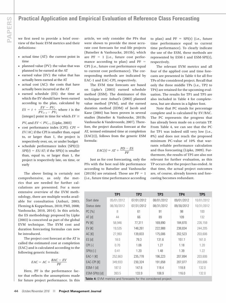
The relevant EVM metrics and all four of the applied cost and time fore-casts are presented in Table 4 for all five TPs of the considered project. Recall that only the three middle TPs (i.e., TP2 to TP4) are retained for the upcoming eval-uation. The results for TP1 and TP5 are also included in Table 4 for complete-ness, but are shown in a lighter font.

Note that PC stands for percentage complete and is calculated by EV/BAC. The PC represents the progress that has already been made on a certain TP. From Table 4, we can see that the PC for TP1 was indeed still very low (i.e., 8%) and does not reach the proposed minimum PC-value of 10% that war-rants reliable performance calculation and thus forecasting (Lipke, 2009). Fur-thermore, the results of TP5 are also not relevant for further evaluation, as this TP occurs after the project has ended. At that time, the actual project outcomes are, of course, already known and fore-casting becomes redundant.

article, we only consider the PFs that were shown to provide the most accu-rate cost forecasts for real-life projects (Batselier & Vanhoucke, 2015b), which are PF 5 1 (i.e., future cost perfor-mance according to plan) and PF 5 CPI (i.e., future cost performance equal to current cost performance). The cor-responding methods are indicated by EAC-1 and EAC-CPI, respectively.

The EVM time forecasts are based on Lipke’s (2003) earned schedule method (ESM). The dominance of this technique over Anbari’s (2003) planned value method (PVM), and the earned duration method (EDM) of Jacob and Kane (2004) has been proven in several studies ( Batselier & Vanhoucke, 2015b; Vanhoucke & Vandevoorde, 2007). There-fore, the project duration forecast at the AT, termed estimated time at completion (EAC(t)), follows from the generic ESM formula:

EAC(t) 5 AT 1 PD 2 ES

PF

Just as for cost forecasting, only the PFs with the best real-life performance according to Batselier and Vanhoucke (2015b) are retained. Those are PF 5 1 (i.e., future time performance according

we first need to provide a brief over-view of the basic EVM metrics and their definitions:

• actual time (AT): the current point in time

• planned value (PV): the value that was planned to be earned at the AT

• earned value (EV): the value that has actually been earned at the AT

• actual cost (AC): the costs that have actually been incurred at the AT

• earned schedule (ES): the time at which the EV should have been earned according to the plan, calculated by

ES 5 t 1 EV 2 PVt

PVt11 2 PVt where t is the

(integer) point in time for which EV $

PVt and EV , PVt11 (Lipke, 2003)• cost performance index (CPI): CPI 5

EV/AC; if the CPI is smaller than, equal to, or larger than 1, the project is respectively over, on, or under budget

• schedule performance index (SPI(t)): SPI(t) 5 ES/AT; if the SPI(t) is smaller than, equal to, or larger than 1, the project is respectively late, on time, or early

The above listing is certainly not comprehensive, as only the met-rics that are needed for further cal-culations are presented. For a more extensive overview of the EVM meth-odology, there are multiple works avail-able for consultation (Anbari, 2003; Fleming & Koppelman, 2010; PMI, 2008; Vanhoucke, 2010, 2014). In this article, the ES methodology proposed by Lipke (2003) is conceived as part of the global EVM technique. The EVM cost and duration forecasting formulas can now be introduced.

The project cost forecast at the AT is called the estimated cost at completion (EAC) and is calculated according to the following generic formula:

EAC 5 AC 1 BAC 2 EV

PF

Here, PF is the performance fac-tor that reflects the assumptions made for future project performance. In this

TP1 TP2 TP3 TP4 TP5Start date 05/01/2012 07/01/2012 08/01/2012 09/01/2012 10/01/2012

Status date 06/30/2012 07/31/2012 08/31/2012 09/30/2012 10/31/2012

PC [%] 8 61 91 98 100

AT [d] 44 66 89 109 132

PV [€] 58,946 77,311 169,890 184,870 226,159

EV [€] 19,535 148,261 222,988 238,834 244,205

AC [€] 27,993 139,833 175,006 202,523 203,606

ES [d] 18.0 79.3 131.6 151.1 161.0

CPI [-] 0.70 1.06 1.27 1.18 1.20

SPI(t) [-] 0.41 1.20 1.48 1.39 1.22

EAC-1 [€] 252,663 235,778 196,223 207,894 203,606

EAC-CPI [€] 349,933 230,324 191,658 207,077 203,606

ESM-1 [d] 187.0 147.6 118.4 118.8 132.0

ESM-SPI(t) [d] 393.5 133.9 108.9 116.0 132.0

Table 4: EVM metrics and forecasts for the considered project.

101278_PMJ_03_036-051.indd 44 9/7/16 10:26 PM


planned, whereas the complete project finished 29 days early. Moreover, most of the predecessors of activity 17 were completed right on time. This means that the buffers introduced in the plan-ning (see Figure 1) were reduced as well and appeared to be oversized. In other words, the start dates of the successor activities could be advanced, as no orga-nizational constraints (e.g., unavailabil-ity of a particular team or subcontractor until a certain date) occurred. Therefore, the project was executed even faster than what would result from shortening the activity durations alone. Because of the large fraction of variable costs in the project, the eventual cost is also reduced significantly, with a magnitude quite similar to the reduction in project dura-tion (i.e., 16.6% compared with 18%).

Now reconsider Table 4. This table shows that it could already be seen from TP2 that the project was going to be both under budget and early, as both the CPI and the SPI(t) were consistently higher than 1. Again, it becomes clear that the progress data of TP1 were not yet reliable, as a CPI of 0.70 and SPI(t) of 0.41 incorrectly indicated that the project—when the performance-based EVM forecasting methods EAC-CPI and ESM-SPI(t) are applied—was going to be well over budget, and even more so, overdue. Furthermore, the RC and RD values could already be observed from the last column of Table 4 (i.e., the post-project forecasts of TP5). Because the RC and RD represent the actual project outcomes and, therefore, the optimal forecast values, they form the basis for evaluating the accuracy of the presented cost and time forecasting methods. More specifically, the mean absolute percentage error (MAPE) mea-sure is used to this end. The generic MAPE formula is as follows:

MAPE 5 1n

n

t51

A2 Ft

A

In this formula, A is the actual (eventual) value and Ft is the forecasted value at time instance t. In our case, the time instances t 5 1,...,n represent

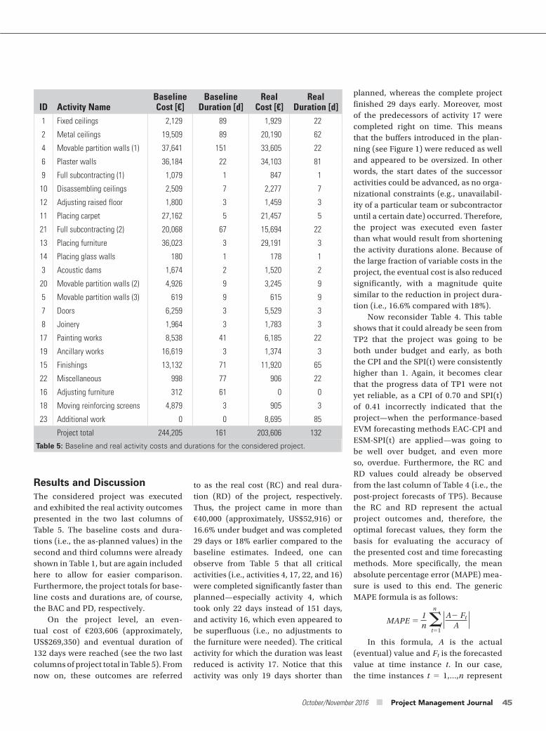
to as the real cost (RC) and real dura-tion (RD) of the project, respectively. Thus, the project came in more than €40,000 (approximately, US$52,916) or 16.6% under budget and was completed 29 days or 18% earlier compared to the baseline estimates. Indeed, one can observe from Table 5 that all critical activities (i.e., activities 4, 17, 22, and 16) were completed significantly faster than planned—especially activity 4, which took only 22 days instead of 151 days, and activity 16, which even appeared to be superfluous (i.e., no adjustments to the furniture were needed). The critical activity for which the duration was least reduced is activity 17. Notice that this activity was only 19 days shorter than

Results and DiscussionThe considered project was executed and exhibited the real activity outcomes presented in the two last columns of Table 5. The baseline costs and dura-tions (i.e., the as-planned values) in the second and third columns were already shown in Table 1, but are again included here to allow for easier comparison. Furthermore, the project totals for base-line costs and durations are, of course, the BAC and PD, respectively.

On the project level, an even-tual cost of €203,606 (approximately, US$269,350) and eventual duration of 132 days were reached (see the two last columns of project total in Table 5). From now on, these outcomes are referred

ID Activity NameBaseline Cost [€]

Baseline Duration [d]

Real Cost [€]

Real Duration [d]

1 Fixed ceilings 2,129 89 1,929 22

2 Metal ceilings 19,509 89 20,190 62

4 Movable partition walls (1) 37,641 151 33,605 22

6 Plaster walls 36,184 22 34,103 81

9 Full subcontracting (1) 1,079 1 847 1

10 Disassembling ceilings 2,509 7 2,277 7

12 Adjusting raised floor 1,800 3 1,459 3

11 Placing carpet 27,162 5 21,457 5

21 Full subcontracting (2) 20,068 67 15,694 22

13 Placing furniture 36,023 3 29,191 3

14 Placing glass walls 180 1 178 1

3 Acoustic dams 1,674 2 1,520 2

20 Movable partition walls (2) 4,926 9 3,245 9

5 Movable partition walls (3) 619 9 615 9

7 Doors 6,259 3 5,529 3

8 Joinery 1,964 3 1,783 3

17 Painting works 8,538 41 6,185 22

19 Ancillary works 16,619 3 1,374 3

15 Finishings 13,132 71 11,920 65

22 Miscellaneous 998 77 906 22

16 Adjusting furniture 312 61 0 0

18 Moving reinforcing screens 4,879 3 905 3

23 Additional work 0 0 8,695 85

Project total 244,205 161 203,606 132

Table 5: Baseline and real activity costs and durations for the considered project.

101278_PMJ_03_036-051.indd 45 9/7/16 10:26 PM



PA

PE

RS

information from past experiences. This also indicates that complete and cor-rect historical data—here, in the form of project manager experience—are crucial to the performance of Monte Carlo sim-ulation. However, for Monte Carlo simu-lation, one needs distributional data for each activity in the project, whereas for RCF, only the general outcomes of simi-lar projects are required. The latter are obviously much easier to obtain, which is an advantage of the RCF technique.

Moreover, Table 6 even shows that RCF with the most specific reference class of projects from the same com-pany (OFW) is the most accurate cost forecasting method of all those consid-ered. It also becomes apparent that the RCF approach needs a reference class consisting of projects that are highly similar to the considered project, as forecasting accuracy clearly dimin-ishes with decreasing similarity level (i.e., from OFW over Comm and Build to Constr). RCF with a reference class comprising all construction projects (Constr) from the database of Batselier and Vanhoucke (2015a) even proves to be the worst-performing method.

Because RCF with reference class OFW is the overall most accurate tech-nique, it also surpasses both EVM cost forecasting methods (which show very similar results). This is remarkable, as the EVM methodology allows forecasts to be updated during project prog-ress (based on actual progress data), whereas RCF only produces one fixed pre-project forecast that remains con-stant throughout the entire project.

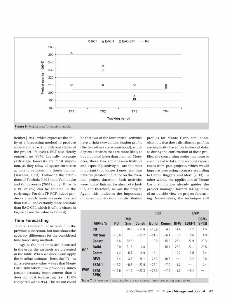
Because RCF yields constant fore-casts, the approach logically exhibits greater forecasting stability than EVM. This is visualized by Figure 5. Since the horizontal line represents the eventual project cost (i.e., RC), the closeness of the markers to this line reflects the forecasting accuracy of the correspond-ing methods (i.e., the closer, the more accurate).

In terms of timeliness (i.e., the third forecasting quality evaluation crite-rion according to Covach, Haydon, and

project considered in this article, as do the presented fore casting results.

Cost ForecastingThe accuracy results for the different cost forecasting methods are presented in Table 6. More specifically, the table shows the difference in MAPEs between the various techniques. A negative number indicates that the horizontal method (row) is more accurate than the vertical method (column), whereas a positive value obviously represents the opposite. All the abbreviations used in the table were already explained earlier in the text.

We will now discuss the results in the order the methods are displayed in Table 6. The BAC represents the pure inside view on project cost forecasting and is used as a first reference value. We see that Monte Carlo simulation yields a more accurate forecast than BAC, albeit modest. The reason that the improvement is only modest might be that symmetrical distribution pro-files were assumed for the uncommon activities, whereas the most important of them (i.e., activities 17, 15, and 16) were executed faster—and thus, more cheaply—than planned. This means that right skewed distribution profiles would have been a better option for those activities, although symmetrical profiles were the more logical choice, given the unavailability of distributional

the n TPs that were selected for the considered project. Furthermore, A is substituted by RC and RD for cost and time forecasting, respectively, and Ft reflects the forecasting outcomes of the different methods. Note, however, that the methodologies of RCF, baseline estimates and Monte Carlo simulation, all produce one fixed forecast prior to the project start that remains constant throughout the entire project. In other words, the forecasts Ft are the same for every TP t (i.e., Ft can be replaced by F). Nevertheless, the MAPE remains a valid accuracy measure in these situa-tions, although its formula is implicitly simplified to |A 2 F|/A (i.e., an absolute percentage error). For the EVM fore-casting methods, on the other hand, the original MAPE formula, of course, continues to apply, with n 5 3 and F1 to F3 reflecting the forecasts for TP2 to TP4. It is always true that the lower the MAPE, the more accurate the forecast-ing method.

In the next two subsections, the per-formance of the considered forecast-ing methods is evaluated—first for cost, and then for time. Thereafter, both fore-casting dimensions are compared more elaborately. Finally, a qualitative discus-sion on the underlying causes for the observed performance of the different forecasting approaches is conducted. Note that this discussion emanates from the specific outcomes of the construction

RCF EVM

[MAPE %] BACMC Sim Constr Build Comm OFW EAC-1 EAC-CPI

BAC — 0.9 26.7 22.9 11.0 16.9 12.8 13.0

MC Sim 20.9 — 27.5 23.8 10.1 16.0 11.9 12.2

RCF

Constr 6.7 7.5 — 3.7 17.7 23.5 19.4 19.7

Build 2.9 3.8 23.7 — 13.9 19.8 15.7 16.0

Comm 211.0 210.1 217.7 213.9 — 5.9 1.8 2.0

OFW 216.9 216.0 223.5 219.8 25.9 — 24.1 23.8

EVMEAC-1 212.8 211.9 219.4 215.7 21.8 4.1 — 0.3

EAC-CPI 213.0 212.2 219.7 216.0 22.0 3.8 20.3 —

Table 6: Difference in accuracy for the considered cost forecasting approaches.

101278_PMJ_03_036-051.indd 46 9/7/16 10:26 PM


profiles for Monte Carlo simulation. Also note that these distribution profiles are implicitly based on historical data, as during the construction of these pro-files, the concerning project manager is encouraged to take into account experi-ences from past projects, which would improve forecasting accuracy according to Caron, Ruggeri, and Merli (2013). In other words, the application of Monte Carlo simulation already guides the project manager toward taking more of an outside view on project forecast-ing. Nevertheless, the technique still

be that two of the four critical activities have a right skewed distribution profile (the two others are symmetrical), which depicts activities that are more likely to be completed faster than planned. More-over, these two activities—activity 22 and especially activity 4—are the most important (i.e., longest) ones, and thus have the greatest influence on the even-tual project duration. Both activities were indeed finished far ahead of sched-ule, and therefore, so was the project. Again, this indicates the importance of correct activity duration distribution

Reither [1981], which expresses the abil-ity of a forecasting method to produce accurate forecasts in different stages of the project life cycle), RCF also clearly outperforms EVM. Logically, accurate early-stage forecasts are most impor-tant, as they allow adequate corrective actions to be taken in a timely manner (Teicholz, 1993). Following the defini-tions of Teicholz (1993) and Vanhoucke and Vandevoorde (2007), only TP1 (with a PC of 8%) can be situated in the early stage. For this TP, RCF indeed pro-duces a much more accurate forecast than EAC-1 and certainly more accurate than EAC-CPI, which is off the charts in Figure 5 (see the value in Table 4).

Time ForecastingTable 7 is very similar to Table 6 in the previous subsection, but now shows the accuracy differences for the considered time forecasting methods.

Again, the outcomes are discussed in the order the methods are presented in the table. When we once again apply the baseline estimate—here, the PD—as a first reference value, we see that Monte Carlo simulation now provides a much greater accuracy improvement than it does for cost forecasting (i.e., 10.6% compared with 0.9%). The reason could

Figure 5: Project cost forecasting results.

TP1 TP2 TP3 TP4

260

RCF EAC-1 EAC-CPI RC

250

Proj

ect c

ost [

x 1,

000

€]

Tracking period

240

230

220

210

200

190

180

RCF EVM

[MAPE %] PDMC Sim Constr Build Comm OFW ESM-1

ESM-SPI(t)

PD — 10.6 211.6 210.9 4.2 14.4 11.2 11.6

MC Sim 210.6 — 222.2 221.5 26.4 3.8 0.6 1.0

RCF

Constr 11.6 22.2 — 0.8 15.9 26.1 22.9 23.3

Build 10.9 21.5 20.8 — 15.1 25.3 22.1 22.5

Comm 24.2 6.4 215.9 215.1 — 10.2 7.0 7.4

OFW 214.4 23.8 226.1 225.3 210.2 — 23.2 22.8

EVMESM-1 211.2 20.6 222.9 222.1 27.0 3.2 — 0.4

ESM-SPI(t)

211.6 21.0 223.3 222.5 27.4 2.8 20.4 —

Table 7: Difference in accuracy for the considered time forecasting approaches.

101278_PMJ_03_036-051.indd 47 9/7/16 10:26 PM



PA

PE

RS

clearly showed the highest accuracy for both dimensions. Traditionally, RCF was introduced to improve the accuracy of cost forecasts and was only applied in this context (Flyvbjerg, 2006; Flyvbjerg & Cowi, 2004). Indeed, our study indi-cates that the technique succeeds in the cost objective, as the BAC (i.e., inside view) and even the periodically updat-ing EVM methods are surpassed in accuracy. On the other hand, RCF has not been applied to time forecasting up to now. Nevertheless, the technique surpasses all other methods for the time dimension in our study. Further-more, compared to cost forecasting, a strongly similar accuracy improvement of the RCF approach, with respect to both the baseline estimate (i.e., PD) and the EVM time forecasting meth-ods could be observed. Specifically, the baseline estimate improvement is only 2.5% smaller for time forecasting (MAPE reduction of 14.4% for PD with respect to 16.9% for BAC), and for the best EVM forecasting method (i.e., ESM-SPI(t) for time and EAC-CPI for cost in this case), the difference even remains limited to 1% (MAPE reduction of 2.8% for ESM-SPI(t) with respect to 3.8% for EAC-CPI). Therefore, our results sug-gest that the RCF approach could just as

The TP1 forecast value for ESM-SPI(t) (see Table 4) is not included in Figure 6 because of the excessive deviation from the eventual outcome, just as for EAC-CPI in Figure 5. The performance-based EVM forecasts (i.e., ESM-SPI(t) and EAC-CPI) thus show a far greater instability than their counterparts, with a PF 5 1.

Comparing Cost and Time ForecastingThe baseline estimates for cost and time forecasting exhibit a very comparable precision, although the PD is slightly less accurate than the BAC (MAPE of 22% compared with 19.9%). On the other hand, Monte Carlo simulation improves the forecasting accuracy for time to a far greater extent than for cost (MAPE reduction of 10.6% compared with 0.9%). The reasons for this were already given in previous subsections. Of course, these reasons are project-specific, and there-fore, the supremacy of Monte Carlo simulation for time with respect to cost should not be generalized.

In this section, we mainly focus on the comparison of the RCF perfor-mance for cost and time forecasting. More specifically, we consider the RCF approach based on the reference class of in-company projects (OFW), which

requires the project manager to make some assumptions (e.g., for activities without precedents).

To completely eliminate human judgment and cut directly to the project outcomes, RCF should be applied. The only concern for this approach regards the selection of an adequate reference class. Our study indicates that, also for time forecasting, a reference class should comprise projects that are suffi-ciently similar to the considered project in order to guarantee accurate forecasts. Indeed, an increasing similarity level of the reference class (i.e., in the order Constr, Build, Comm, and OFW) results in increasing forecasting accuracy.

Moreover, when applying RCF with the most specific reference class of in-company projects (OFW), both EVM methods are outperformed in nearly equal measure. This outcome corresponds per-fectly to that for cost forecasting. This is also the case for the comparison between RCF and EVM in terms of stability and timeliness, as for time forecasting, RCF also surpasses EVM. This can be ascer-tained from Figure 6, which should be interpreted in the exact same way as Figure 5. The theoretical explanation was already provided in the previous subsec-tion and is therefore not repeated here.

TP1 TP2 TP3 TP4

190

180

170

Proj

ect d

urat

ion

[day

s]

Tracking period

160

150

140

130

120

110

100

RCF ESM-1 ESM-SPI(t) RD

Figure 6: Project duration forecasting results.

101278_PMJ_03_036-051.indd 48 9/7/16 10:26 PM


of all these forecasting methods dem-onstrates that the RCF technique is the most user-friendly, as it does not require a great deal of detailed information (such as distributional data about activ-ity durations for Monte Carlo simula-tion) or extensive calculations (like the periodical forecast updates for EVM).

Moreover, although RCF produces pre-project forecasts that remain con-stant throughout project execution (just like baseline estimates and Monte Carlo simulation), it surpasses all the tradi-tional techniques in accuracy, stabil-ity, and timeliness. The dominance of RCF in accuracy is especially remark-able, as the competing EVM technique yields forecasts that are updated dur-ing project progress. Furthermore, the strong performance of RCF occurs for both cost and time forecasting, and in nearly equal measure. Therefore, our study suggests that RCF could have the same merits for time forecasting as for cost forecasting, for which the technique had already been applied (Flyvbjerg, 2006; Flyvbjerg & Cowi, 2004). However, RCF only outperforms the other techniques when the degree of similarity between the considered project and the projects in the refer-ence class is sufficiently high. More concretely, in our case, the reference class had to consist of projects from the same finishing construction com-pany. A clear decrease in forecasting accuracy could be observed with the gradually declining similarity level of the reference class.

In our specific case, the qualitative reason for the dominance of the outside view on project forecasting over the traditional inside view could be found in the occurrence of a newly identi-fied type of strategic misinterpretation, which suggests that project managers in the post-approval phase are inclined to overestimate the expected costs and durations so that their targets (and bonuses) could be achieved more easily.

This article supports the practi-cal relevance of applying RCF for real-life projects and also shows how the

been approved, and therefore, under-estimating costs and durations would not offer advantages. On the contrary, it would only force the project manag-ers to work faster and more cheaply in order to reach the set goals and the possible bonuses that go with them. Consequently, it is plausible and per-haps even natural that these project managers—with their projects already approved and assigned to them—would rather overestimate the foreseen costs and durations (and build in buffers) so that their targets—and the correspond-ing bonuses—could be achieved more easily. The exact nature and the effect of strategic misinterpretation thus appear to depend on the phase the project is in when preparing the plan (i.e., produc-ing the baseline estimates): The preap-proval phase leads to underestimations, whereas the post-approval phases causes overestimations. Furthermore, the fact that many activities that were planned behind a buffer could actually be started before their foreseen start date not only indicates the absence of organizational constraints (e.g., unavail-ability of a particular team or subcon-tractor until a certain date), but also supports the idea of post-approval stra-tegic misinterpretation having occurred for the considered project. In any event, the RCF technique (i.e., outside view) can bypass the biasing effects of this new type of strategic misinterpretation, as our study has shown.

ConclusionsThe main objective of this article was to support the practical relevance of RCF by applying the technique to a real-life project and quantitatively evaluating it through comparison with the most commonly used traditional forecasting methods. More specifically, the consid-ered real-life project is a finishing con-struction project that was selected from the database of Batselier and Vanhoucke (2015a). The forecasting techniques with which RCF was compared are baseline estimates, Monte Carlo simulation, and EVM. First, practical application

well have merit for forecasting project duration.

Qualitative DiscussionPrevious studies (Flyvbjerg, Holm, & Buhl, 2002; 2005; Kahneman & Tversky, 1979b; Lovallo & Kahneman, 2003; Wachs, 1989, 1990) have argued that people—and, therefore, project managers—generally tend to underestimate costs (and dura-tions) when applying an inside view to project forecasting. They identified two reasons: optimism bias (i.e., uninten-tionally seeing future events in a more positive light than warranted by actual experience) and strategic misinterpreta-tion (i.e., deliberately and strategically making more positive predictions so as to give the impression that the com-petition would be surpassed). However, when looking at the baseline estimates (i.e., inside view) for the considered project and for similar projects within the same finishing construction com-pany (reference class OFW), we observed exactly the opposite—namely, a struc-tural overestimation of costs and dura-tions. This cannot be explained by the existence of an unintended “negativism bias” (i.e., seeing future events in a more negative light than warranted by actual experience), as this would be in contradic-tion with the usual manifestations of the human psyche according to the research of Kahneman and Tversky (1979b) and Lovallo and Kahneman (2003). In other words, negativism bias cannot exist alongside positivism bias; they would, by definition, be mutually exclusive. There-fore, strategic misinterpretation must be the root of the structural overestimations within the considered company.

Note that strategic misinterpreta-tion, as also presented by Flyvbjerg (2006), is traditionally defined for the preapproval phase of a project. Project managers would benefit from underes-timating costs and durations by increas-ing the chance of their project—and not that of the competition—would be approved (and funded). However, all considered projects of the finish-ing construction company had already

101278_PMJ_03_036-051.indd 49 9/7/16 10:26 PM



PA

PE

RS

Fleming, Q., & Koppelman, J. (2010). Earned value project management (4th ed.). Newtown Square, PA: Project Management Institute.

Flyvbjerg, B. (2006). From Nobel Prize to project management: Getting risks right. Project Management Journal, 37(3), 5–15.

Flyvbjerg, B. (2007). Eliminating bias in early project development through reference class forecasting and good governance. In K. J. Sunnevåg (Ed.), Decisions based on weak information: Approaches and challenges in the early phase of projects (pp. 90–110). Trondheim, Norway: Concept Program, The Norwegian University of Science and Technology.

Flyvbjerg, B., & Cowi. (2004). Procedures for dealing with optimism bias in transport planning: Guidance document. London, England: UK Department for Transport.

Flyvbjerg, B., Holm, M., & Buhl, S. (2002). Underestimating costs in public works projects: Error or lie? Journal of the American Planning Association, 68(3), 279–295.

Flyvbjerg, B., Holm, M., & Buhl, S. (2005). How (in)accurate are demand forecasts in public works projects? The case of transportation. Journal of the American Planning Association, 71(2), 131–146.

Jacob, D., & Kane, M. (2004). Forecasting schedule completion using earned value metrics? Revisited. The Measurable News (Summer), 11–17.

Kahneman, D. (1994). New challenges to the rationality assuption. Journal of Institutional and Theoretical Economics, 150(1), 18–36.

Kahneman, D., & Tversky, A. (1979a). Intuitive prediction: Biases and corrective procedures. In S. Makridakis & S. Wheelwright (Eds.), Studies in the management sciences: Forecasting (p. 12). Amsterdam, Netherlands: North Holland.

Kahneman, D., & Tversky, A. (1979b). Prospect theory: An analysis of decisions under risk. Econometrica, 47 (2), 313–327.

practical applicability and utility of RCF, but also of many other project manage-ment techniques.

AcknowledgmentsWe acknowledge the support provided by the “Nationale Bank van België” (NBB) and by the “Bijzonder Onderzoeksfonds” (BOF) for the project with contract number BOF12GOA021. Furthermore, we would also like to thank Gilles Bonne, Eveline Hoogstoel, and Gilles Vandewiele for their efforts in developing PMConverter.

ReferencesAnbari, F. (2003). Earned value project management method and extensions. Project Management Journal, 34 (4), 12–23.

Batselier, J., & Vanhoucke, M. (2015a). Construction and evaluation framework for a real-life project database. International Journal of Project Management, 33(3), 697–710.

Batselier, J., & Vanhoucke, M. (2015b). Empirical evaluation of earned value management forecasting accuracy for time and cost. Journal of Construction Engineering and Management, 141(11), 05015010.

Carbone, R., & Armstrong, J. (1982). Evaluation of extrapolative forecasting methods: Results of a survey of academicians and practitioners. Journal of Forecasting, 1(2), 215–217.

Caron, F., Ruggeri, F., & Merli, A. (2013). A Bayesian approach to improve estimate at completion in earned value management. Project Management Journal, 44(1), 3–16.

Colin, J., & Vanhoucke, M. (2016). Empirical perspective on activity durations for project management simulation studies. Journal of Construction Engineering and Management, 142(1), 04015047.

Covach, J., Haydon, J., & Reither, R. (1981). A study to determine indicators and methods to compute estimate at completion (EAC). Fairfax, VA: ManTech International Corporation.

technique can be evaluated on a quan-titative basis through comparison with other existing forecasting methods. Although this study provides interesting insights into the workings and perfor-mance of RCF and other forecasting methods, its results may not be readily generalized because of the restricted number of real-life projects from which the reference classes were selected. To increasingly substantiate the valid-ity of the RCF technique, it should be applied and tested on an ever-growing empirical project database.

Furthermore, following the con-cept of combining outside view with inside view for project forecasting (Kim & Reinschmidt, 2011), we identify the future research topic of integrating RCF in EVM. By replacing the baseline estimates with the forecasts from RCF, more accurate EVM performance met-rics could be obtained. In turn, this would lead to more reliable warning sig-nals and thus more adequate corrective actions. Therefore, it would ensure more effective project control in general. This assertion should, of course, be validated by extensive empirical research.

Although the RCF technique in itself is fairly straightforward, it is relatively difficult to correctly implement in prac-tice because of its strong dependence on the selected reference class. As this research has shown, a reference class of (highly) similar projects is needed to provide (highly) accurate forecasts. Such a collection of (highly) similar projects is not always readily available in practice. Even less often is the collec-tion of adequate size; indeed, forecast-ing bias increases as the reference class gets smaller, which can undermine the performance and applicability of RCF. That is why it is of great importance to have available many (and correct) real-life project data. Organizations should make a point of collecting their proj-ects’ progress and performance data in a structured way, as described, for example, in Batselier and Vanhoucke (2015a) or at www.or-as.be/research/database. This would not only boost the

101278_PMJ_03_036-051.indd 50 9/7/16 10:26 PM


evaluation, a real-life project database—freely available at www.or-as.be/research/database—was created under his guidance. He has presented his work at several international conferences on project management and operational research in cities that include Rome, Italy; Barcelona, Spain; Munich, Germany; and Ghent, Belgium. He can be contacted at [email protected]

Mario Vanhoucke is a full professor at Ghent University (Belgium), Vlerick Business School (Belgium, Russia, China), and UCL (University College London) School of Management (UK). He has a PhD in operations management (2001) and a master’s degree in business engineering from the University of Leuven (Belgium). He teaches Project Management, Business Statistics, and Decision Sciences for Business and Applied Operations Research, and is also a guest lecturer in the Beijing MBA program at Peking University (China). His main research interest lies in the integration of project scheduling, risk management, and project control using combinatorial optimization models. He is an advisor for several PhD projects, has published more than 60 papers in international journals, and is the author of four project management books published by Springer. He is a regular guest on international conferences as an invited speaker or chairman and a reviewer of numerous articles submitted for publication in international academic journals. He is a founding member and director of the EVM Europe Association (www.evm-europe.eu) and partner at the company OR-AS (www.or-as.be). His project management research has received multiple awards, including the 2008 International Project Management Association (IPMA) Research Award for his research project Measuring Time—A Project Performance Simulation Study, which was received at the IPMA world congress held in Rome, Italy. He also received the Notable Contributions to Management Accounting Literature Award from the American Accounting Association at their 2010 conference in Denver, Colorado, USA. He can be contacted at [email protected]

Vanhoucke, M., & Vandevoorde, S. (2007). A simulation and evaluation of earned value metrics to forecast the project duration. Journal of the Operational Research Society, 58(10), 1361–1374.

Wachs, M. (1989). When planners lie with numbers. Journal of the American Planning Association, 55(4), 476–479.

Wachs, M. (1990). Ethics and advocacy in forecasting for public policy. Business and Professional Ethics Journal, 9(1–2), 141–157.

Warburton, R. (2011). A time-dependent earned value model for software projects. International Journal of Project Management, 29(8), 1082–1090.

Willems, L., & Vanhoucke, M. (2015). Classification of articles and journals on project control and earned value management. International Journal of Project Management, 33(7), 1610–1634.

Jordy Batselier holds master’s degrees in civil engineering (2011) and business economics (2012) from Ghent University (Belgium). Since 2012 he has been working as a PhD researcher at the Operations Research & Scheduling research group of the Faculty of Economics and Business Administration of Ghent University. He is a teaching assistant for business games in project management courses and supervises multiple master’s students during the completion of their dissertations. Furthermore, he is co-developer of the project management software tool PMConverter (available at www.or-as.be/research/database). His research interest lies in project management, and more specifically, in performing project control by means of earned value management. His specific research actions are focused on the empirical evaluation and development of forecasting techniques for project duration and cost, on which he has published several papers in international journals. For the empirical

Kim, B., & Reinschmidt, K. (2011). Combination of project cost forecasts in earned value management. Journal of Construction Engineering and Management, 137(11), 958–966.

Lipke, W. (2003). Schedule is different. The Measurable News (Summer), 31–34.

Lipke, W. (2009). Project duration forecasting . . . A comparison of earned value management methods to earned schedule. The Measurable News, (2), 24-31.

Lovallo, D., & Kahneman, D. (2003, July). Delusions of success: How optimism undermines executives’ decisions. Harvard Business Review, 56–63.

Project Management Institute. (PMI). (2008). A guide to the project management body of knowledge (PMBOK® guide) – Third Edition. Newtown Square, PA: Author.

Teicholz, P. (1993). Forecasting final cost and budget of construction projects. Journal of Computing in Civil Engineering, 7(4), 511–529.

Trietsch, D., Mazmanyan, L., Gevorgyan, L., & Baker, K. (2012). Modeling activity times by the Parkinson distribution with a lognormal core: Theory and validation. European Journal of Operational Research, 216(2), 386–396.

Vanhoucke, M. (2010). Measuring time-improving project performance using earned value management (Vol. 136 of International Series in Operations Research and Management Science). New York, NY: Springer.

Vanhoucke, M. (2014). Integrated project management and control: First comes the theory, then the practice (Vol. Management for Professionals). New York, NY: Springer.

101278_PMJ_03_036-051.indd 51 9/7/16 10:26 PM

This material has been reproduced with the permission of the copyright owner. Unauthorized reproduction of this material is strictly prohibited. For permission to

reproduce this material, please contact PMI.

practical application and empirical evaluation of reference class forecasting...

Documents