powerpc 970 programming environment - ibm · pdf fileiv ibm eserver bladecenter js20 powerpc...

ibm.com/redbooks Redpaper

IBM

IBM Eserver BladeCenter JS20PowerPC 970 Programming Environment

Ben GibbsRobert Arenburg

Damien BonaventureBradley ElkinRogeli Grima

Amy Wang

PowerPC 970 microprocessors

Vector Multimedia Extensions (VMX)

Optimization and performance considerations

http://www.redbooks.ibm.com/


International Technical Support Organization

IBM Eserver BladeCenter JS20 PowerPC 970 Programming Environment

January 2005

© Copyright International Business Machines Corporation 2005. All rights reserved.Note to U.S. Government Users Restricted Rights -- Use, duplication or disclosure restricted by GSA ADP ScheduleContract with IBM Corp.

First Edition (January 2005)

This edition applies to the IBM Eserver BladeCenter JS2 and the IBM PowerPC 970 and 970FX microprocessors.

Note: Before using this information and the product it supports, read the information in “Notices” on page vii.

Contents

Notices . . . . . . . . . . . . . . . . . . . . . . . . . . . . . . . . . . . . . . . . . . . . . . . . . . . . . . . . . . . . . . . . . viiTrademarks . . . . . . . . . . . . . . . . . . . . . . . . . . . . . . . . . . . . . . . . . . . . . . . . . . . . . . . . . . . . . viii

Preface . . . . . . . . . . . . . . . . . . . . . . . . . . . . . . . . . . . . . . . . . . . . . . . . . . . . . . . . . . . . . . . . . ixThe team that wrote this Redpaper . . . . . . . . . . . . . . . . . . . . . . . . . . . . . . . . . . . . . . . . . . . . ixBecome a published author . . . . . . . . . . . . . . . . . . . . . . . . . . . . . . . . . . . . . . . . . . . . . . . . . . .xComments welcome. . . . . . . . . . . . . . . . . . . . . . . . . . . . . . . . . . . . . . . . . . . . . . . . . . . . . . . . xi

Part 1. Overview of the PowerPC 970 Microprocessor . . . . . . . . . . . . . . . . . . . . . . . . . . . . . . . . . . . . . . . 1

Chapter 1. Introduction to the PowerPC 970 features . . . . . . . . . . . . . . . . . . . . . . . . . . . 31.1 Overview . . . . . . . . . . . . . . . . . . . . . . . . . . . . . . . . . . . . . . . . . . . . . . . . . . . . . . . . . . . . . 41.2 Programming environment . . . . . . . . . . . . . . . . . . . . . . . . . . . . . . . . . . . . . . . . . . . . . . . 91.3 Data types . . . . . . . . . . . . . . . . . . . . . . . . . . . . . . . . . . . . . . . . . . . . . . . . . . . . . . . . . . . 101.4 Support for 32-bit and 64-bit . . . . . . . . . . . . . . . . . . . . . . . . . . . . . . . . . . . . . . . . . . . . . 111.5 Register sets . . . . . . . . . . . . . . . . . . . . . . . . . . . . . . . . . . . . . . . . . . . . . . . . . . . . . . . . . 12

1.5.1 User-level registers . . . . . . . . . . . . . . . . . . . . . . . . . . . . . . . . . . . . . . . . . . . . . . . . 141.5.2 Supervisor-level registers . . . . . . . . . . . . . . . . . . . . . . . . . . . . . . . . . . . . . . . . . . . 141.5.3 Machine state register. . . . . . . . . . . . . . . . . . . . . . . . . . . . . . . . . . . . . . . . . . . . . . 17

1.6 PowerPC instructions . . . . . . . . . . . . . . . . . . . . . . . . . . . . . . . . . . . . . . . . . . . . . . . . . . 191.6.1 Code example for a digital signal processing filter . . . . . . . . . . . . . . . . . . . . . . . . 21

1.7 Superscalar and pipelining . . . . . . . . . . . . . . . . . . . . . . . . . . . . . . . . . . . . . . . . . . . . . . 221.8 Application binary interface . . . . . . . . . . . . . . . . . . . . . . . . . . . . . . . . . . . . . . . . . . . . . . 241.9 The stack frame . . . . . . . . . . . . . . . . . . . . . . . . . . . . . . . . . . . . . . . . . . . . . . . . . . . . . . 291.10 Parameter passing . . . . . . . . . . . . . . . . . . . . . . . . . . . . . . . . . . . . . . . . . . . . . . . . . . . 311.11 Return values . . . . . . . . . . . . . . . . . . . . . . . . . . . . . . . . . . . . . . . . . . . . . . . . . . . . . . . 331.12 Summary. . . . . . . . . . . . . . . . . . . . . . . . . . . . . . . . . . . . . . . . . . . . . . . . . . . . . . . . . . . 34

Chapter 2. VMX in the PowerPC 970 . . . . . . . . . . . . . . . . . . . . . . . . . . . . . . . . . . . . . . . . 352.1 Vectorization overview . . . . . . . . . . . . . . . . . . . . . . . . . . . . . . . . . . . . . . . . . . . . . . . . . 36

2.1.1 Vector technology review . . . . . . . . . . . . . . . . . . . . . . . . . . . . . . . . . . . . . . . . . . . 382.2 Vector memory addressing . . . . . . . . . . . . . . . . . . . . . . . . . . . . . . . . . . . . . . . . . . . . . . 422.3 Instruction categories . . . . . . . . . . . . . . . . . . . . . . . . . . . . . . . . . . . . . . . . . . . . . . . . . . 47

Part 2. VMX programming environment . . . . . . . . . . . . . . . . . . . . . . . . . . . . . . . . . . . . . . . . . . . . . . . . . . 51

Chapter 3. VMX programming basics . . . . . . . . . . . . . . . . . . . . . . . . . . . . . . . . . . . . . . . 533.1 Programming guidelines . . . . . . . . . . . . . . . . . . . . . . . . . . . . . . . . . . . . . . . . . . . . . . . . 54

3.1.1 Automatic vectorization versus hand coding. . . . . . . . . . . . . . . . . . . . . . . . . . . . . 543.1.2 Language-specific issues . . . . . . . . . . . . . . . . . . . . . . . . . . . . . . . . . . . . . . . . . . . 543.1.3 Use of math libraries . . . . . . . . . . . . . . . . . . . . . . . . . . . . . . . . . . . . . . . . . . . . . . . 553.1.4 Performance tips . . . . . . . . . . . . . . . . . . . . . . . . . . . . . . . . . . . . . . . . . . . . . . . . . . 553.1.5 Issues and suggested remedies . . . . . . . . . . . . . . . . . . . . . . . . . . . . . . . . . . . . . . 563.1.6 VAST code optimizer . . . . . . . . . . . . . . . . . . . . . . . . . . . . . . . . . . . . . . . . . . . . . . 583.1.7 Summary of programming guidelines . . . . . . . . . . . . . . . . . . . . . . . . . . . . . . . . . . 58

3.2 Vector data types . . . . . . . . . . . . . . . . . . . . . . . . . . . . . . . . . . . . . . . . . . . . . . . . . . . . . 593.3 Vector keywords . . . . . . . . . . . . . . . . . . . . . . . . . . . . . . . . . . . . . . . . . . . . . . . . . . . . . . 603.4 VMX C extensions. . . . . . . . . . . . . . . . . . . . . . . . . . . . . . . . . . . . . . . . . . . . . . . . . . . . . 61

3.4.1 Extensions to printf() and scanf() . . . . . . . . . . . . . . . . . . . . . . . . . . . . . . . . . . . . . 61

© Copyright IBM Corp. 2005. All rights reserved. iii

3.4.2 Input conversion specifications . . . . . . . . . . . . . . . . . . . . . . . . . . . . . . . . . . . . . . . 623.4.3 Vector functions . . . . . . . . . . . . . . . . . . . . . . . . . . . . . . . . . . . . . . . . . . . . . . . . . . 643.4.4 Summary of VMX C extensions . . . . . . . . . . . . . . . . . . . . . . . . . . . . . . . . . . . . . . 68

Chapter 4. Application development tools . . . . . . . . . . . . . . . . . . . . . . . . . . . . . . . . . . . 694.1 GNU compiler collection . . . . . . . . . . . . . . . . . . . . . . . . . . . . . . . . . . . . . . . . . . . . . . . . 70

4.1.1 Processor-specific compiler options . . . . . . . . . . . . . . . . . . . . . . . . . . . . . . . . . . . 704.1.2 Compiler options for VMX . . . . . . . . . . . . . . . . . . . . . . . . . . . . . . . . . . . . . . . . . . . 704.1.3 Suggested compiler options . . . . . . . . . . . . . . . . . . . . . . . . . . . . . . . . . . . . . . . . . 71

4.2 XL C/C++ and XL FORTRAN compiler collections . . . . . . . . . . . . . . . . . . . . . . . . . . . . 714.2.1 Options controlling vector code generation. . . . . . . . . . . . . . . . . . . . . . . . . . . . . . 734.2.2 Alignment-related attributes and builtins . . . . . . . . . . . . . . . . . . . . . . . . . . . . . . . . 734.2.3 Data dependency analysis . . . . . . . . . . . . . . . . . . . . . . . . . . . . . . . . . . . . . . . . . . 764.2.4 Useful pragmas. . . . . . . . . . . . . . . . . . . . . . . . . . . . . . . . . . . . . . . . . . . . . . . . . . . 794.2.5 Generating vectorization reports . . . . . . . . . . . . . . . . . . . . . . . . . . . . . . . . . . . . . . 80

Chapter 5. Vectorization examples . . . . . . . . . . . . . . . . . . . . . . . . . . . . . . . . . . . . . . . . . 835.1 Explanation of the examples . . . . . . . . . . . . . . . . . . . . . . . . . . . . . . . . . . . . . . . . . . . . . 84

5.1.1 Command-line options . . . . . . . . . . . . . . . . . . . . . . . . . . . . . . . . . . . . . . . . . . . . . 855.2 Vectorized loops . . . . . . . . . . . . . . . . . . . . . . . . . . . . . . . . . . . . . . . . . . . . . . . . . . . . . . 85

5.2.1 SAXPY example . . . . . . . . . . . . . . . . . . . . . . . . . . . . . . . . . . . . . . . . . . . . . . . . . . 865.2.2 Reduction loop . . . . . . . . . . . . . . . . . . . . . . . . . . . . . . . . . . . . . . . . . . . . . . . . . . . 885.2.3 Variation of the reduction loop . . . . . . . . . . . . . . . . . . . . . . . . . . . . . . . . . . . . . . . 895.2.4 Dot product . . . . . . . . . . . . . . . . . . . . . . . . . . . . . . . . . . . . . . . . . . . . . . . . . . . . . . 925.2.5 Byte clamping . . . . . . . . . . . . . . . . . . . . . . . . . . . . . . . . . . . . . . . . . . . . . . . . . . . . 945.2.6 Summary. . . . . . . . . . . . . . . . . . . . . . . . . . . . . . . . . . . . . . . . . . . . . . . . . . . . . . . . 98

Chapter 6. A case study . . . . . . . . . . . . . . . . . . . . . . . . . . . . . . . . . . . . . . . . . . . . . . . . . . 996.1 Introducing vector code in your application. . . . . . . . . . . . . . . . . . . . . . . . . . . . . . . . . 100

6.1.1 Appropriate uses of vectorization . . . . . . . . . . . . . . . . . . . . . . . . . . . . . . . . . . . . 1016.1.2 Analyzing data types. . . . . . . . . . . . . . . . . . . . . . . . . . . . . . . . . . . . . . . . . . . . . . 1026.1.3 Introducing vector code in the algorithm . . . . . . . . . . . . . . . . . . . . . . . . . . . . . . . 1036.1.4 Conclusions . . . . . . . . . . . . . . . . . . . . . . . . . . . . . . . . . . . . . . . . . . . . . . . . . . . . 107

Appendix A. Code listings . . . . . . . . . . . . . . . . . . . . . . . . . . . . . . . . . . . . . . . . . . . . . . . 109Code examples . . . . . . . . . . . . . . . . . . . . . . . . . . . . . . . . . . . . . . . . . . . . . . . . . . . . . . . . . 109Code loops from Toronto Labs VAC test suite . . . . . . . . . . . . . . . . . . . . . . . . . . . . . . . . . . 110

Appendix B. Porting from Apple OS X . . . . . . . . . . . . . . . . . . . . . . . . . . . . . . . . . . . . . 113Compiler Flags . . . . . . . . . . . . . . . . . . . . . . . . . . . . . . . . . . . . . . . . . . . . . . . . . . . . . . . . . . 113Initialization Syntax . . . . . . . . . . . . . . . . . . . . . . . . . . . . . . . . . . . . . . . . . . . . . . . . . . . . . . 113Best Practices . . . . . . . . . . . . . . . . . . . . . . . . . . . . . . . . . . . . . . . . . . . . . . . . . . . . . . . . . . 114IBM Visual Age. . . . . . . . . . . . . . . . . . . . . . . . . . . . . . . . . . . . . . . . . . . . . . . . . . . . . . . . . . 115References. . . . . . . . . . . . . . . . . . . . . . . . . . . . . . . . . . . . . . . . . . . . . . . . . . . . . . . . . . . . . 115

Appendix C. Additional material . . . . . . . . . . . . . . . . . . . . . . . . . . . . . . . . . . . . . . . . . . 117Locating the Web material . . . . . . . . . . . . . . . . . . . . . . . . . . . . . . . . . . . . . . . . . . . . . . . . . 117Using the Web material . . . . . . . . . . . . . . . . . . . . . . . . . . . . . . . . . . . . . . . . . . . . . . . . . . . 117

System requirements for downloading the Web material . . . . . . . . . . . . . . . . . . . . . . . 118How to use the Web material . . . . . . . . . . . . . . . . . . . . . . . . . . . . . . . . . . . . . . . . . . . . 118

Related publications . . . . . . . . . . . . . . . . . . . . . . . . . . . . . . . . . . . . . . . . . . . . . . . . . . . . 119IBM Redbooks . . . . . . . . . . . . . . . . . . . . . . . . . . . . . . . . . . . . . . . . . . . . . . . . . . . . . . . . . . 119Other publications . . . . . . . . . . . . . . . . . . . . . . . . . . . . . . . . . . . . . . . . . . . . . . . . . . . . . . . 119Online resources . . . . . . . . . . . . . . . . . . . . . . . . . . . . . . . . . . . . . . . . . . . . . . . . . . . . . . . . 120

iv IBM Eserver BladeCenter JS20 PowerPC 970 Programming Environment

How to get IBM Redbooks . . . . . . . . . . . . . . . . . . . . . . . . . . . . . . . . . . . . . . . . . . . . . . . . . 120Help from IBM . . . . . . . . . . . . . . . . . . . . . . . . . . . . . . . . . . . . . . . . . . . . . . . . . . . . . . . . . . 120

Index . . . . . . . . . . . . . . . . . . . . . . . . . . . . . . . . . . . . . . . . . . . . . . . . . . . . . . . . . . . . . . . . . 121

Contents v

vi IBM Eserver BladeCenter JS20 PowerPC 970 Programming Environment

Notices

This information was developed for products and services offered in the U.S.A.

IBM may not offer the products, services, or features discussed in this document in other countries. Consult your local IBM representative for information on the products and services currently available in your area. Any reference to an IBM product, program, or service is not intended to state or imply that only that IBM product, program, or service may be used. Any functionally equivalent product, program, or service that does not infringe any IBM intellectual property right may be used instead. However, it is the user's responsibility to evaluate and verify the operation of any non-IBM product, program, or service.

IBM may have patents or pending patent applications covering subject matter described in this document. The furnishing of this document does not give you any license to these patents. You can send license inquiries, in writing, to: IBM Director of Licensing, IBM Corporation, North Castle Drive Armonk, NY 10504-1785 U.S.A.

The following paragraph does not apply to the United Kingdom or any other country where such provisions are inconsistent with local law: INTERNATIONAL BUSINESS MACHINES CORPORATION PROVIDES THIS PUBLICATION "AS IS" WITHOUT WARRANTY OF ANY KIND, EITHER EXPRESS OR IMPLIED, INCLUDING, BUT NOT LIMITED TO, THE IMPLIED WARRANTIES OF NON-INFRINGEMENT, MERCHANTABILITY OR FITNESS FOR A PARTICULAR PURPOSE. Some states do not allow disclaimer of express or implied warranties in certain transactions, therefore, this statement may not apply to you.

This information could include technical inaccuracies or typographical errors. Changes are periodically made to the information herein; these changes will be incorporated in new editions of the publication. IBM may make improvements and/or changes in the product(s) and/or the program(s) described in this publication at any time without notice.

Any references in this information to non-IBM Web sites are provided for convenience only and do not in any manner serve as an endorsement of those Web sites. The materials at those Web sites are not part of the materials for this IBM product and use of those Web sites is at your own risk.

IBM may use or distribute any of the information you supply in any way it believes appropriate without incurring any obligation to you.

Information concerning non-IBM products was obtained from the suppliers of those products, their published announcements or other publicly available sources. IBM has not tested those products and cannot confirm the accuracy of performance, compatibility or any other claims related to non-IBM products. Questions on the capabilities of non-IBM products should be addressed to the suppliers of those products.

This information contains examples of data and reports used in daily business operations. To illustrate them as completely as possible, the examples include the names of individuals, companies, brands, and products. All of these names are fictitious and any similarity to the names and addresses used by an actual business enterprise is entirely coincidental.

COPYRIGHT LICENSE: This information contains sample application programs in source language, which illustrates programming techniques on various operating platforms. You may copy, modify, and distribute these sample programs in any form without payment to IBM, for the purposes of developing, using, marketing or distributing application programs conforming to the application programming interface for the operating platform for which the sample programs are written. These examples have not been thoroughly tested under all conditions. IBM, therefore, cannot guarantee or imply reliability, serviceability, or function of these programs. You may copy, modify, and distribute these sample programs in any form without payment to IBM for the purposes of developing, using, marketing, or distributing application programs conforming to IBM's application programming interfaces.

© Copyright IBM Corp. 2005. All rights reserved. vii

TrademarksThe following terms are trademarks of the International Business Machines Corporation in the United States, other countries, or both:

Eserver®Eserver®ibm.com®pSeries®AIX®BladeCenter™DB2®Hypervisor™

IBM®Lotus®PowerOpen™PowerPC Architecture™PowerPC 604™PowerPC®POWER™POWER3™

POWER4™POWER5™Redbooks™Redbooks (logo) ™Tivoli®3890™

The following terms are trademarks of other companies:

Power MAC™ is a trademark of the Apple Computer Corporation.

AltiVec™ is a trademark of Motorola.

Linux is a trademark of Linus Torvalds in the United States, other countries, or both.

Other company, product, and service names may be trademarks or service marks of others.

viii IBM Eserver BladeCenter JS20 PowerPC 970 Programming Environment

Preface

This Redpaper gives a broad understanding of the programming environment of the IBM® PowerPC® 970 microprocessor that is implemented in the IBM Eserver® BladeCenter™ JS20. It also provides information about how to take advantage of the Vector Multimedia Extensions (VMX) execution unit found in the PowerPC 970 to increase the performance of applications in 3D graphics, modelling and simulation, digital signal processing, and others.

The audience for this Redpaper is application programmers and software engineers who want to port code to the PowerPC 970 microprocessor to take advantage of the VMX performance gains.

The team that wrote this RedpaperThis Redpaper was produced by a team of specialists from around the world working at the International Technical Support Organization (ITSO), Austin Center.

Ben Gibbs is a Senior Consulting Engineer with Technonics, Inc. (http://www.technonics.com) in Austin, Texas. He has been involved with the POWER™ and PowerPC family of microprocessors and embedded controllers since 1989. The past seven years he has been working with the Microelectronics Division at IBM, providing training on the PowerPC embedded controllers and microprocessors. He was the project leader for this IBM Redpaper.

Robert Arenburg is a Senior Technical Consultant in the Solutions Enablement organization in the IBM Systems and Technology Group located in Austin, Texas, and he has worked at IBM for 13 years. He has a Ph.D. in Engineering Mechanics from Virginia Tech. His areas of expertise include high performance computing, performance, capacity planning, 3D graphics, solid mechanics, as well as computational and finite element methods.

Damien Bonaventure is an Advisory Software Engineer in the Toronto Software Lab. He has been with the TOBEY Optimizing backend team for seven years. His experiences include working on code generation techniques for both IBM and non-IBM systems such as Solaris and Mac OSX and implementing optimizations such as the Basis Block Instruction Scheduler for the POWER4™. He also has experience analyzing code performance at the instruction level. He was the TOBEY team lead for the IBM XL compiler port to Mac OSX, which was the first XL compiler product to feature support for VMX. He holds a Bachelor of Applied Science in Computer Engineering from the University of Toronto.

Bradley Elkin is a Senior Software Engineer for IBM. He holds a Ph.D. in Chemical Engineering from the University of Pennsylvania and has 17 years of experience in high performance computing. His areas of expertise include applications from computational fluid mechanics, computational chemistry, and bioinformatics. He has written several articles for IBM Eserver Development Domain.

Note: The PowerPC 970 microprocessor is available from the IBM Microelectronics Division for companies wanting to implement a PowerPC microprocessor into their embedded applications or other designs. The information in this paper will be helpful for those firmware and software engineers responsible for supporting their product. The Apple Power Mac G5 system also uses the PowerPC 970 microprocessor and application programmers can find the information within this paper useful.

© Copyright IBM Corp. 2005. All rights reserved. ix

http://www.technonics.com

Rogeli Grima is a research staff member at the CEPBA IBM Research Institute in Spain. He has three years of experience in applied mathematics. He has also collaborated on the development of JS20 blade server solution for bioinformatics.

Amy Wang obtained her Bachelor of Applied Science degree in 1999, specializing in Computer Engineering offered under the Engineering Science faculty at the University of Toronto. In the fall of 2001, she completed her Master of Applied Science degree in Computer Engineering at the University of Toronto. In 2002, she joined the IBM Toronto Software Lab, contributing her skills to the development of various compiler backend optimizations. Currently, she is working with the IBM Watson research team to implement automatic simdization, which will enable automatic VMX code generation for the JS20 hardware.

Thanks to the following people for their contributions to this project:

Chris Blatchley, Lupe Brown, Arzu Gucer, and Scott VetterITSO, Austin Center

Omkhar ArasaratnamIBM Toronto Canada

James KellyIBM Melbourne Australia

Randy SwanbergIBM Austin

Become a published authorJoin us for a two- to six-week residency program! Help write an IBM Redbook dealing with specific products or solutions, while getting hands-on experience with leading-edge technologies. You'll team with IBM technical professionals, Business Partners or customers.

Your efforts will help increase product acceptance and customer satisfaction. As a bonus, you'll develop a network of contacts in IBM development labs, and increase your productivity and marketability.

Find out more about the residency program, browse the residency index, and apply online at:

ibm.com/redbooks/residencies.html

x IBM Eserver BladeCenter JS20 PowerPC 970 Programming Environment

http://www.redbooks.ibm.com/residencies.html

http://www.redbooks.ibm.com/residencies.html

Comments welcomeYour comments are important to us!

We want our papers to be as helpful as possible. Send us your comments about this Redpaper or other Redbooks™ in one of the following ways:

� Use the online Contact us review redbook form found at:

ibm.com/redbooks

� Send your comments in an email to:

[email protected]

� Mail your comments to:

IBM Corporation, International Technical Support OrganizationDept. JN9B Building 90511501 Burnet RoadAustin, Texas 78758-3493

Preface xi



http://www.redbooks.ibm.com/contacts.html

xii IBM Eserver BladeCenter JS20 PowerPC 970 Programming Environment

Part 1 Overview of the PowerPC 970 Microprocessorcroprocessor

This section reviews the PowerPC 64-bit architecture as it applies to the PowerPC 970 microprocessor. Chapter 1 describes the features, instructions, instruction pipelines, programming environment, data types, register sets, and application binary interface specification. Chapter 2 focuses on the Vector Multimedia Extension (VMX) implementation in the PowerPC 970 and includes a discussion of VMX technology, instruction categories, and memory addressing.

Part 1

© Copyright IBM Corp. 2005. All rights reserved. 1

2 IBM Eserver BladeCenter JS20 PowerPC 970 Programming Environment

Chapter 1. Introduction to the PowerPC 970 features

The IBM PowerPC 970 Reduced Instruction Set Computer (RISC) microprocessor is an implementation of the PowerPC Architecture™. This chapter provides an overview of the PowerPC 970 features, including a block diagram showing the major functional components. It also provides information about how 970 implementation complies with the PowerPC architecture definition.

1

Note: This paper uses the term PowerPC 970 to refer to both the IBM PowerPC 970 and IBM PowerPC 970FX microprocessors. Also, it uses the term JS20 blade to refer to the IBM Eserver BladeCenter JS20.

Fact: Altvec is used by Motorola, Velocity Engine is used by Apple, and VMX is used by IBM to refer to the PowerPC vector execution unit such as the one implemented in the PowerPC 970 microprocessor.


1.1 OverviewThe PowerPC 970 is a 64-bit PowerPC RISC microprocessor with VMX extensions. VMX extensions are single-instruction, multiple-data (SIMD) operations that accelerate data intensive processing tasks. This processor is designed to support multiple system configurations ranging from desktop and low-end server applications uniprocessor up through a 4-way simultaneous multiprocessor (SMP). The JS20 blades use the PowerPC 970 in a 2-way SMP configuration.

The PowerPC 970 is comprised of three main components:

� PowerPC 970 core, which includes VMX execution units

� PowerPC 970 storage (STS), which includes core interface logic, non-cacheable unit, L2 cache and controls, and the bus interface unit

� 970 Pervasive functions

The PowerPC 970 microprocessor consists of the following features:

� 64-bit implementation of the PowerPC AS Architecture (version 2.0)

– Binary compatibility for all PowerPC AS application level code (problem state)

– Binary compatibility for all PowerPC application level code (problem state)

– N-1 operating system capable for AIX® and Linux

– Support for 32-bit operating system bridge facility

– Vector/SIMD Multimedia Extension (VMX)

� Layered implementation strategy for very high frequency operation

– 64 KB direct-mapped instruction cache

• 128 byte cache lines

– Deeply pipelined design

• Fetch of eight instructions on eight-word boundaries per cycle

• 16 stages for most fixed-point register-register operations

• 18 stages for most load and store operations (assuming L1 Dcache hit)

• 21 stages for most floating point operations

• 19, 22, and 25 stages for fixed-point, complex-fixed, and floating point operations, respectively in the VALU.

• 19 stages for VMX permute operations

– Dynamic instruction cracking for some instructions allows for simpler inner core dataflow

• Dedicated dataflow for cracking one instruction into two internal operations

• Microcoded templates for longer emulation sequences


� Speculative superscalar inner core organization

– Aggressive branch prediction

• Scan all eight fetched instructions for branches each cycle

• Predict up to two branches per cycle (if the first one is predicted fall-through)

• 32-entry count cache for address prediction (indexed by address of bcctr instructions)

• Support for up to 16 predicted branches in flight

• Prediction support for branch direction and branch addresses

– In order dispatch of up to five operations into distributed issue queue structure

– Out of order issue of up to 10 operations into 10 execution pipelines

• Two load or store operations

• Two fixed-point register-register operations

• Two floating-point operations

• One branch operation

• One condition register operation

• One VMX permute operation

• One VMX ALU operation

– Capable of restoring the machine state for any of the instructions in flight

• Very fast restoration for instructions on group boundaries (that is, branches)

• Slower for instructions contained within a group

– Register renaming on GPRs, FPRs, VRFs, CR Fields, XER (parts), FPSCR, VSCR, Link and Count

• 80-entry GPR rename mapper (32 architected GPRs plus four eGPRs)

• 80-entry FPR rename mapper (32 architected FPRs)

• 80-entry VRF rename mapper (32 architected VRFs)

• 24-entry XER rename mapper (XER broken into four mappable fields and one non-mappable)

• Mappable fields: ov, ca/oc, fxcc, tgcc

• Non-mappable bits: dc, ds, string-count, other_bits

• Special fields (value predict): so

• 16-entry LR/CTR rename mapper (one LR and one CTR)

• 32-entry CR rename mapper (eight CR fields plus one eCR field)

• 20-entry FPSCR rename mapper

• No register renaming on: MSR, SRR0, SRR1, DEC, TB, HID0, HID1, HID4, SDR1, DAR, DSISR, CTRL, SPRG0, SPRG1, SPRG2, SPRG3, ASR, PVR, PIR, SCOMC, SCOMD, ACCR, CTRL, DABR, VSCR, or PerfMon registers

Chapter 1. Introduction to the PowerPC 970 features 5

– Instruction queuing resources:

• Two, 18-entry issue queues for fixed-point and load/store instructions

• Two, 10-entry issue queues for floating-point instructions

• 12-entry issue queue for branches instructions

• 10-entry issue queue for CR-logical instructions

• 16-entry issue queue for Vector Permute instructions

• 20-entry issue queue for Vector ALU instructions and VMX Stores

� Large number of instructions in flight (theoretical maximum of 215 instructions)

– Up to 16 instructions in instruction fetch unit (fetch buffer and overflow buffer)

– Up to 32 instructions in instruction fetch buffer in instruction decode unit

– Up to 35 instructions in three decode pipe stages and four dispatch buffers

– Up to 100 instructions in the inner-core (after dispatch)

– Up to 32 stores queued in the STQ (available for forwarding)

– Fast, selective flush of incorrect speculative instructions and results

� Vector Multimedia eXtension (VMX) execution pipelines

– Two dispatchable units:

• VALU contains three subunits:

Vector simple fixed: 1-stage execution

Vector complex fixed: 4-stage execution

Vector floating point: 7-stage execution

• VPERM - 1-stage execution

– Out-of-order issue with bias towards oldest operations first

– Symmetric forwarding between the permute and VALU pipelines

� Specific focus on storage latency management

– 32 KB, two-way set associative data cache

• 128 byte cache line, FIFO replacement policy

• Triple ported to support two reads and one write every cycle

• Two cycle load-to-use (cycles between load instruction and able to used by dependent structure) penalty for FXU loads

• Four cycle load-to-use penalty for FPU loads

• Three cycle load-to-use penalty for VMX VPERM loads

• Four cycle load-to-use penalty for VMX VALU loads

– Out-of-order and speculative issue of load operations

– Support for up to eight outstanding L1 cache line misses

– Hardware initiated instruction prefetching from L2 cache

– Software initiated data stream prefetching with support for up to eight active streams

– Critical word forwarding and critical sector first

– New branch processing and prediction hints for branch instructions


� L2 Cache Features

– 512KB size, eight-way set associative

– Fully inclusive of L1 data cache

– Unified L2 cache controller (instructions, data, page table entries, and so on)

– Store-in L2 cache (store-through L1 cache)

– Fully integrated cache, tags, and controller

– Five-state modified, exclusive, recent, shared, and invalid (MERSI) coherency protocol

– Runs at core frequency (1:1)

– Handle all cacheable loads/stores (including lwarx/stcwx)

– Critical octaword forwarding on data loads

– Critical octaword forwarding in instruction fetches

� Power management

– Doze, nap, and deep nap capabilities

– Static power management

• Software initiated doze and nap mode

– Dynamic power management

• Parts of the design stop their (hardware initiated) clocks when not in use

– PowerTune

• Software initiated slow down of the processor; selectable to half or quarter of the nominal operating frequency

� Storage Subsystem (STS)

– Encompasses the Core Interface Unit, Non-Cachable Unit (NCU), the L2 cache controller and 512KB L2 cache, and the Bus Interface Unit (BIU)


Figure 1-1 shows the block diagram of the PowerPC 970 core.

Figure 1-1 PowerPC 970 block diagram

64KBInstruction

Cache

InstructionFetch Unit

InstructionDecode Unit

Dispatch Buffer

Register Maps - GPR, FPR, VRF, CR, CTR, LK

GlobalCompletion

Table

CRIssue Queue

BRIssue Queue

FPUIssue Queue

VMX PermuteIssue Queue

VMX ALUIssue Queue

FX1/LSU1Issue Queue

FX2/LSU2Issue Queue

CR

CR RF

BR

CTR/LK

FP1 FP2

FPR

FX1 LS1

GPR

FX2 LS2

GPR

VPERM

VRF

VALU

VRF

32KBDataCache

Core Interface Unit

NCUL2 Dir/Cntl512KB L2 Cache

Bus Interface Unit

PowerPC 970 Bus

PowerPC 970 Core

STS


1.2 Programming environmentThe programming environment consists of the resources that are accessible from the processor running in problem state mode (non-supervisory), which is called user mode by the operating system.. The PowerPC architecture is a load-store architecture that defines specifications for both 32-bit and 64-bit implementations. The PowerPC 970 is a 64-bit implementation. The instruction set is partitioned into four functional classes: branch, fixed-point, floating-point, and VMX.

The registers are also partitioned into groups corresponding to these classes. That is, there are condition code and branch target registers for branches, floating-point registers for floating-point operations, general-purpose registers for fixed-point operations, and vector registers for VMX operations.

This partition benefits superscalar implementations by reducing the interlocking necessary for dependency checking. The explicit indication of all operands in the instructions, combined with the partitioning of the PowerPC architecture into functional classes, exposes dependences to the compiler. Although instructions must be word (32-bit) aligned, data can be misaligned within certain implementation-dependent constraints.

The floating-point facilities support compliance to the IEEE 754 Standard for Binary Floating-Point Arithmetic (IEEE 754).

In 64-bit implementations, such as the PowerPC 970, two modes of operation are determined by the 64-bit mode (SF) bit in the Machine State Register: 64-bit mode (SF set to 1) and 32-bit mode (SF cleared to 0), for compatibility with 32-bit implementations. Application code for 32-bit implementations executes without modification on 64-bit implementations running in 32-bit mode, yielding identical results. All 64-bit implementation instructions are available in both modes. Identical instructions, however, can produce different results in 32-bit and 64-bit modes. Differences between 32-bit and 64-bit mode include but are not limited to:

� Addressing

Although effective addresses in 64-bit implementations have 64 bits, in 32-bit mode, the high-order 32 bits are ignored during data access and set to zero during instruction fetching. This modification of the high-order bits of the address might produce an unexpected jump following the transition from 64-bit mode to 32-bit mode.

� Status bits

The register result of arithmetic and logical instructions is independent of mode, but setting of status bits depends on the mode. In particular, recording, carry-bit–setting, or overflow-bit–setting instruction forms write the status bits relative to the mode. Changing the mode in the middle of a code sequence that depends on one of these status bits can lead to unexpected results.

� Count Register

The entire 64-bit value in the Count Register of a 64-bit implementation is decremented, even though conditional branches in 32-bit mode only test the low-order 32 bits for zero.


1.3 Data typesThe PowerPC 64-bit architecture supports the data types shown in Table 1-1. The basic data types are byte (8-bit), halfword (16-bits), word (32-bits), and doubleword (64-bits) for fixed-point operations. The floating-point types are single-precision (32-bits) and double-precision (64-bits). Vector data types are quadwords (128-bits).

Table 1-1 PowerPC 64-bit data types

Type ANSI C Size (bytes)

Alignment PowerPC

Boolean _bool 1 byte unsigned byte

Character charunsigned char

1 byte unsigned byte

signed char 1 byte signed byte

shortsigned short

2 halfword signed halfword

unsigned short 2 halfword unsigned halfword

Integral intsigned intenum

4 word signed word

unsigned int 4 word unsigned word

long intsigned longlong long

8 doubleword signed doubleword

unsigned longunsigned long long

8 doubleword unsigned doubleword

__int128_t 16 quadword signed quadword

__unit128_t 16 doubleword unsigned quadword

Pointer any *any (*) ()

8 doubleword unsigned doubleword

Floating-point float 4 word single precision

double 8 doubleword double precision

long double 16 quadword extended precision

Vector 16*char 16 quadword vector of signed bytes

16*unsigned char 16 quadword vector of unsigned bytes

8*short 16 quadword vector of signed shorts

8*unsigned short 16 quadword vector of unsigned shorts

4*int 16 quadword vector of signed words

4*unsigned int 16 quadword vector of unsigned words

4*float 16 quadword vector of floats


In Table 1-1 on page 10, extended precision is the AIX 128-bit long double format composed of two double-precision numbers with different magnitudes that do not overlap. The high-order double-precision value (the one that comes first in storage) must have the larger magnitude. The value of the extended-precision number is the sum of the two double-precision values and include the following features:

� Extended precision provides the same range of double precision (about 10**(-308) to 10**308) but more precision (a variable amount, about 31 decimal digits or more).

� As the absolute value of the magnitude decreases (near the denormal range), the precision available in the low-order double also decreases.

� When the value represented is in the denormal range, this representation provides no more precision than 64-bit (double) floating point.

� The actual number of bits of precision can vary. If the low-order part is much less then 1 ULP of the high-order part, significant bits (either all 0's or all 1's) are implied between the significands of high-order and low-order numbers. Some algorithms that rely on having a fixed number of bits in the significand can fail when using extended precision.

This extended precision differs from the IEEE 754 in the following ways:

� Software support is restricted to round-to-nearest mode. Programs that use extended precision must ensure that this rounding mode is in effect when extended-precision calculations are performed.

� The software does not fully support the IEEE special numbers not-a-number and INF. These values are encoded in the high-order double value only. The low-order value is not significant.

� The software does not support the IEEE status flags for overflow, underflow, and other conditions. These flags have no meaning in this format.

1.4 Support for 32-bit and 64-bitThe PowerPC 970 uses the same data paths and execution units for both 32-bit and 64-bit operations. There are no limitations or reduced performance situations due to running applications in 32-bit mode. There is no “compatibility” or “emulation” mode. Whether the processor is in 32-bit mode or 64-bit mode is controlled by the MSR[SF] bit. (See Table 1-2 on page 17 for a description of the machine state register.)

The PowerPC architecture was defined from the beginning to be a 64-bit architecture and the 32-bit implementations of the PowerPC architecture are subsets. For example, the PowerPC 604e microprocessor implemented in the IBM pSeries® 43P-150 workstation is a 32-bit PowerPC microprocessor. This microprocessor can execute all the instructions in the PowerPC architecture except those that involve the doubleword (64-bit) operands such as ld (load doubleword). Nothing would prevent the operating system from trapping and emulating these 64-bit instructions, being completely transparent to the application. Another example of this is the lwz (load word and zero) instruction.


On the PowerPC 970, a 32-bit word is loaded from memory into the instruction-specified 64-bit general-purpose register and the upper 32-bits of the register are set to zero (cleared). On the PowerPC 604e the same instruction is executed, and the same word loaded into the same register. However, there is nothing to zero because the register is 32-bits on this microprocessor. For the most part, binary compatibility exists between the 32-bit and 64-bit PowerPC microprocessors. When it becomes time for a customer to migrate their applications from 32-bit IBM Eserver pSeries systems to the 64-bit IBM Eserver BladeCenter JS20, the porting effort can be minimal. This cannot be said for many other architectures today.

1.5 Register setsRegisters are defined at all three levels of the PowerPC architecture, namely user instruction set architecture (UISA), virtual environment architecture (VEA), and operating environment architecture (OEA). The PowerPC architecture defines register-to-register operations for all computational instructions. Source data for these instructions are accessed from the on-chip registers or are provided as immediate values embedded in the opcode. The three-register instruction format allows specification of a target register distinct from the two source registers, thus preserving the original data for use by other instructions and reducing the number of instructions required for certain operations. Data is transferred between memory and registers with explicit load and store instructions only. Figure 1-2 on page 13 shows the registers found in the PowerPC 970.

PowerPC processors have two levels of privilege: supervisor mode of operation (typically used by the operating system) and user mode of operation (used by the application software, it is also called problem state).

The programming models incorporate 32 general-purpose registers, 32 floating-point registers, 32 vector registers, special-purpose registers, and several miscellaneous registers. Each PowerPC microprocessor also has its own unique set of hardware implementation-dependent (HID) registers.

While running in supervisor mode. the operating system is able to execute all instructions and access all registers defined in the PowerPC Architecture. In this mode, the operating system establishes all address translations and protection mechanisms, loads all processor state registers. and sets up all other control mechanisms defined on the 970 processor. While running in user mode (problem state), many of these registers and facilities are not accessible, and any attempt to read or write these register results in a program exception.


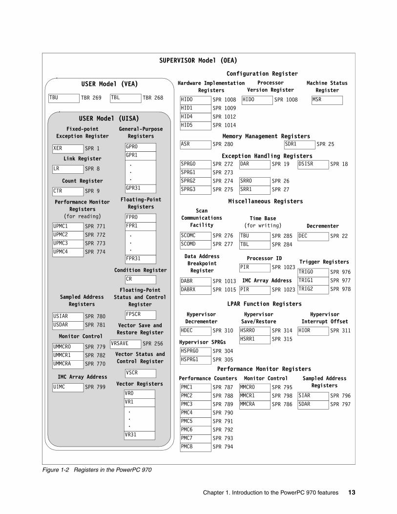
Figure 1-2 Registers in the PowerPC 970

TBU TBR 269 TBL TBR 268

CTR SPR 9

Count Register

XER SPR 1

Fixed-point Exception Register

LR SPR 8

Link Register

USER Model (UISA)

GPR0GPR1...

GPR31

General-Purpose Registers

FPR0FPR1...

FPR31

Floating-Point Registers

CRCondition Register

FPSCR

Floating-Point Status and Control

Register

Vector Save and Restore Register

VSCR

VR0VR1...

VR31

Vector Registers

UPMC1 SPR 771

Performance Monitor Registers

(for reading)

UPMC2 SPR 772UPMC3 SPR 773UPMC4 SPR 774

HIDO SPR 1008HID1 SPR 1009HID4 SPR 1012HID5 SPR 1014

USIAR SPR 780

Sampled Address Registers

USDAR SPR 781

UMMCR0 SPR 779

Monitor Control

UMMCR1 SPR 782

VRSAVE SPR 256

Vector Status and Control RegisterUMMCRA SPR 770

UIMC SPR 799

IMC Array Address

USER Model (VEA)

SUPERVISOR Model (OEA)

Hardware Implementation Registers

Configuration RegisterProcessor

Version Register

HIDO SPR 1008

Machine Status Register

MSR

Memory Management RegistersASR SPR 280 SDR1 SPR 25

Exception Handling RegistersSPRG0 SPR 272 DAR SPR 19 DSISR SPR 18SPRG1 SPR 273SPRG2 SPR 274SPRG3 SPR 275

SRR0 SPR 26SRR1 SPR 27

Miscellaneous RegistersScan

Communications Facility

SCOMC SPR 276SCOMD SPR 277

TBU SPR 285TBL SPR 284

Time Base(for writing)

DEC SPR 22

Decrementer

Data Address Breakpoint Register

DABR SPR 1013DABRX SPR 1015

Processor IDPIR SPR 1023

PIR SPR 1023

IMC Array AddressTRIG0 SPR 976TRIG1 SPR 977TRIG2 SPR 978

Trigger Registers

LPAR Function Registers

Hypervisor Decrementer

HDEC SPR 310

Hypervisor Save/RestoreHSRR0 SPR 314HSRR1 SPR 315

Hypervisor Interrupt Offset

HIOR SPR 311

Hypervisor SPRGsHSPRG0 SPR 304HSPRG1 SPR 305

Performance Monitor Registers

PMC1 SPR 787PMC2 SPR 788PMC3 SPR 789PMC4 SPR 790

Performance Counters

PMC5 SPR 791PMC6 SPR 792PMC7 SPR 793PMC8 SPR 794

MMCR0 SPR 795MMCR1 SPR 798MMCRA SPR 786

Monitor Control Sampled Address Registers

SIAR SPR 796SDAR SPR 797


1.5.1 User-level registersThe user-level registers can be accessed by all software with either user or supervisor privileges and include the following registers:

� General-purpose registers (GPRs). The thirty-two 64-bit GPRs (GPR0–GPR31) serve as data source or destination registers for integer instructions and provide data for generating addresses.

� Floating-point registers (FPRs). The thirty-two 64-bit FPRs (FPR0–FPR31) serve as the data source or destination for all floating-point instructions.

� Condition register (CR). The 32-bit CR consists of eight 4-bit fields (CR0–CR7) that reflect results of certain arithmetic operations and provide a mechanism for testing and branching.

� Floating-point status and control register (FPSCR). The FPSCR contains all floating-point exception signal bits, exception summary bits, exception enable bits, and rounding control bits that are needed for compliance with the IEEE 754.

� Vector registers (VRs). The VR file consists of thirty-two 128-bit VRs (VR0-VR31). The VRs serve as vector source and vector destination registers for all vector instructions.

� Vector status and control register (VSCR). The VSCR contains the non-Java and saturation bit. The remaining bits are reserved.

� Vector save and restore register (VRSAVE). The VRSAVE assists the application and operating system software in saving and restoring the architectural state across context-switched events.

The remaining user-level registers are special purpose registers (SPRs). The PowerPC architecture provides a separate mechanism for accessing SPRs (the mtspr and mfspr instructions). These instructions are commonly used to explicitly access certain registers, while other SPRs can be accessed more typically as the side effect of executing other instructions.

For a detailed description of the GPRs, FPRs, CR, and FPSCR, consult PowerPC Microprocessor Family: The Programming Environments available at either of the following Web addresses:

http://www.chips.ibm.comhttp://www.technonics.com/powerpc/publications

For information about the VRs, see PowerPC Microprocessor Family: AltiVec Technology Programming Environments, also available at these addresses.

1.5.2 Supervisor-level registersThe PowerPC OEA defines the registers that an operating system uses for memory management, configuration, exception handling, and other operating system functions.

The OEA defines the following supervisor-level registers for 32-bit implementations:

� Configuration registers

– Machine state register (MSR). The MSR defines the state of the processor. The MSR can be modified by the Move to Machine State Register (mtmsr) System Call (sc) instructions and the Return from Exception (rfi) instruction. The MSR can be read by the Move from Machine State Register (mfmsr) instruction. When an exception is taken, the contents of the MSR are saved to the machine status save and restore register 1 (SRR1), described in the bulleted list that follows.


http://www.chips.ibm.com

http://www.technonics.com/powerpc/publications

For information about the MSR, see the PowerPC Microprocessor Family: The Programming Environments manual available either of the following Web addresses:

http://www.chips.ibm.comhttp://www.technonics.com/powerpc/publications

– Processor version register (PVR). The PVR is a read-only register that identifies the version (model) and revision level of the PowerPC processor. For more information, refer to the PowerPC 970 datasheet.The processor revision level (PVR[16:31]) starts at x‘0100’, indicating revision ‘1.0’. As revisions are made, bits [29:31) indicate minor revisions. Similarly, bits [20:23] indicate major changes. Bits [16:19] are a technology indicator. Bits [24:27] are reserved for future use.

� Memory management registers

– Address space register (ASR). In the PowerPC 970, the ASR is supported and is considered a hypervisor resource. Due to the software reload of the SLBs on the 970FX, this register does not actually participate in any other specific hardware functions on the chip. It has been included as a convenience (and performance enhancement) for the SLB reload software.

– Storage description register (SDR1). The SDR1 holds the page table base address used in virtual-to-physical address translation.

� Exception-handling registers

– Data address register (DAR). After a DSI or an alignment exception, the DAR is set to the effective address generated by the faulting instruction.

– Software use SPRs (SPRG0–SPRG3). SPRG0–SPRG3 are provided for operating system use. These registers are not architecturally defined and also are not found in all POWER and PowerPC microprocessors. They might or might not be used by the operating system. Their ideal use is for servicing interrupts and used as scratch pad registers. The point here is that level-0 storage (registers) are faster to access than level-1 storage (L1 cache), level-2 storage (L2 caches), and so on.

– Data storage interrupt status register (DSISR). The bits in the DSISR reflect the cause of DSI and alignment exceptions.

– Machine status save and restore register 0 (SRR0). The SRR0 is used to save the address of the instruction at which normal execution resumes when the rfi instruction executes at the end of an exception handler routine.

– Machine status save and restore register 1 (SRR1). The SRR1 is a 64-bit register used to save machine status on exceptions and restore machine status register when an rfid instruction is executed. In the 970FX, bits [2], [4:32], [34], [37-41], [57], [60], and [63] are treated as reserved. These bits are not implemented and return the value 0b0 when read.

Important: The MSR is defined by the PowerPC architecture. However, the bit definitions can change from one PowerPC microprocessor type to another. The PowerPC 970 user’s manual describes the actual bit implementation of the MSR.

Note: The processor version number (PVR[0:15]) for the PowerPC 970 is 0x0039. In future versions of the PowerPC 970, this section of the version number will only change if there are significant software-visible changes in the design.


http://www.technonics.com/powerpc/publications


� Miscellaneous registers

– Time base (TB). The TB is a 64-bit structure provided for maintaining the time of day and operating interval timers. The TB consists of two 32-bit registers: time base upper (TBU) and time base lower (TBL). The time base registers can be written to only by supervisor-level software but can be read by both user and supervisor-level software.

– Decrementer register (DEC). The DEC is a 32-bit decremented counter that provides a mechanism for causing a decrementer exception after a programmable delay; the frequency is a subdivision of the processor clock.

– Data address breakpoint register (DABR). The DABR register is used to cause a breakpoint exception if a specified data address is encountered.

– Processor ID register (PIR). The PIR is used to differentiate between individual processors in a multiprocessor environment.

� PowerPC 970-specific registers

The PowerPC architecture allows implementation-specific SPRs. Those incorporated in the PowerPC 970 are described as follows.

– Instruction address breakpoint (IABR). The PowerPC 970 does not support a software visible form of the instruction address breakpoint facility. As a debug feature that is accessible via the support processor interface, it does support an instruction breakpoint feature.

– Hardware implementation-dependent register 0 (HID0). The HID0 controls various functions, such as enabling checkstop conditions, and locking, enabling, and invalidating the instruction and data caches, power modes, miss-under-miss, and others. This register is hypervisor write access and privileged read access only.

– Hardware implementation-dependent register 1 (HID1). The HID1 contains additional mode bits that are related to the instruction fetch and instruction decode functions in the PowerPC 970. This register is hypervisor write access and privileged read access only.

– Hardware implementation-dependent register 4 (HID4) and hardware implementation-dependent register 5 (HID5).The HID4 and HID5 contain bits related to LPAR and the load-store function in the PowerPC 970. All of these registers are hypervisor write access and privileged read access only.

– Performance monitor registers. The following registers are used to define and count events for use by the performance monitor:

• The performance monitor counter registers (PMC1–PMC8) are used to record the number of times a certain event has occurred. UPMC1–UPMC8 provide user-level read access to these registers.

• The monitor mode control registers (MMCR0, MMCR1, MMCRA) are used to enable various performance monitor interrupt functions. UMMCR0, UMMCR1, UMMCRA provide user-level read access to these registers.

• The sampled instruction address register (SIAR) contains the effective address of an instruction executing at or around the time that the processor signals the performance monitor interrupt condition.

• The sampled data address register (SDAR) contains the effective address of the storage access instruction.

Note: While it is not guaranteed that the implementation of PowerPC 970-specific registers is consistent among PowerPC processors, other processors can implement similar or identical registers.


1.5.3 Machine state registerThe machine state register (MSR) is a 64-bit register on 64-bit PowerPC implementations and a 32-bit register in 32-bit PowerPC implementations. The MSR on the PowerPC 970 is a 64-bit register. The MSR defines the state of the processor. When an exception occurs, the contents of the MSR register are saved in SRR1 or, when a hypervisor interrupt occurs, are saved in HSRR1. A new set of bits are loaded into the MSR as determined by the exception. The MSR can also be modified by the mtmsrd (or mtmsr), sc, rfid or hrfid instructions. It can be read by the mfmsr instruction.

Figure 1-3 shows the format of this register. Table 1-2 describes the bits. Bits 1 through 37, 39 through 44, 46, 47, 56, 60, 61, and 63 are reserved bits and return 0b0 when read.

Figure 1-3 Machine State Register (MSR)

Table 1-2 MSR bit settings

0 0 0000....000 37 38 39 40 41 42 43 44 45 46 47 48 49 50 51 52 53 54 55 56 57 58 59 60 61 62 63

SF POW

VMX EE

PR

FP

ME

FE0

SE

BE

FE1

IP

IR

DR

RI

Bit Name Description

0 SF Sixty-four bit mode0 The processor runs in 32-bit mode1 The processor runs in 64-bit mode

1:37 Reserved bits

38 VMX VMX execution unit enable0 VMX execution unit disabled1 VMX execution enabled

39:44 Reserved bits

45 POW Power management enable0 Power management disabled (normal operation mode)1 Power management enabled (reduced power mode)

46:47 Reserved bits

48 EE External interrupt enable0 Processor is not preempted by external interrupts or decrementer1 Processor is enabled to take external and decremeter interrupts

49 PR Privilege level (Problem state mode)0 Processor is in supervisory mode (AIX or Linux kernel/system mode)1 Processor is in non-supervisory mode (AIX or linux user mode)

50 FP Floating-point enable0 Floating-point execution unit is disabled1 Floating-point execution unit is enabled

51 ME Machine check enable0 Machine check exceptions are disabled1 Machine check exceptions are enabled


The default state of this register coming out of reset is that all the bits of the MSR are cleared except bits 0 (SF) and 57 (IP) which are set to one (1). Therefore, the PowerPC 970 begins in 64-bit mode and fetches the first instruction from 0xFFFF_FFFF_FFF0_0100 (system reset vector).

52 FE0 Floating-point exception mode 0Used with bit 55 (FE1) to:

FE0 FE1 Mode0 0 Floating-point exceptions are disabled0 1 Floating-point imprecise nonrecoverable1 0 Floating-point imprecise recoverable1 1 Floating-point precise mode

53 SE Single-step trace enable0 The processor executes instructions normally1 The processor generates a single-step trace exception (debugging)

54 BE Branch trace enable0 The processor executes branch instructions normally1 The processor generates a branch trace exception at the completion

of a branch instruction, regardless of whether the branch was taken

55 FE1 Floating-point exception mode 1See bit 52 (FE0) for details

56 Reserved bit

57 IP Interrupt prefix0 Interrupts are vectored to the real address of 0x0000_0000_000n_nnnn1 Interrupts are vectored to the real address of 0xFFFF_FFFF_FFFn_nnnnNote: This bit is automatically set (1) during reset and then cleared (0) by firmware after the operating system has been loaded relative to real address 0x0000_0000_0000_0000

58 IR Instruction address translation0 Instruction address translation is disabled (real mode)1 Instruction address translation is enabled (virtual mode)

59 DR Data address translation0 Data address translation is disabled (real mode)1 Data address translation is enabled (virtual mode)

60:61 Reserved bits

62 RI Recoverable exception0 Exception is not recoverable1 Exception is recoverable

63 Reserved bit

Bit Name Description


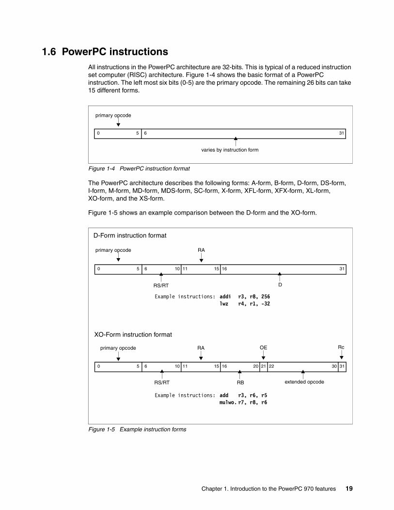
1.6 PowerPC instructionsAll instructions in the PowerPC architecture are 32-bits. This is typical of a reduced instruction set computer (RISC) architecture. Figure 1-4 shows the basic format of a PowerPC instruction. The left most six bits (0-5) are the primary opcode. The remaining 26 bits can take 15 different forms.

Figure 1-4 PowerPC instruction format

The PowerPC architecture describes the following forms: A-form, B-form, D-form, DS-form, I-form, M-form, MD-form, MDS-form, SC-form, X-form, XFL-form, XFX-form, XL-form, XO-form, and the XS-form.

Figure 1-5 shows an example comparison between the D-form and the XO-form.

Figure 1-5 Example instruction forms

0 5 6 31

primary opcode

varies by instruction form

0 5 6 10 11 15 16 31

primary opcode

RS/RT

RA

D

0 5 6 10 11 15 16 20 21 22 30 31

D-Form instruction format

XO-Form instruction format

primary opcode

RS/RT

RA

RB

OE

extended opcode

Rc

Example instructions: addi r3, r8, 256lwz r4, r1, -32

Example instructions: add r3, r6, r5mulwo. r7, r8, r6


In Figure 1-5 on page 19, the instruction addi r3, r8, 256 has:

� Bits 0 through 5 encoded with the bit value of 0b001110 (14) as the primary opcode.� Bits 6 through 10 encoded with 0b00011 (3) for GPR 3.� Bits 11 through 15 encoded with 0b01000 (8) for GPR 8.� Bits 16 through 31 contain 0b0000000100000000 (256), a 16-bit signed two’s complement

integer that is extended to 64 bits during execution.

During the execution of this instruction, the contents of GPR 8 are added to 256 and the results placed into GPR 3.

The instruction lwz r4, r3, -32 has:

� Bits 0 through 5 encoded with the bit value of 0b100000 (32) as the primary opcode.� Bits 6 through 10 encoded with 0b00100 (4) for GPR 4.� Bits 11 through 15 encoded with 0b00001 (1) for GPR 1.� Bits 16 through 31 contain 0b1111111111100000 (-32), a 16-bit signed two’s complement

integer that is extended to 64 bits during execution.

During the execution of this instruction, the contents of GPR 1 are added to the immediate value (-32) to form the effective address.

If address translation is enabled (MSR[DR] = 1), the effective address is translated to a real address and the 32-bit word at that address is placed into GPR 4, along with the upper 32-bits of the 64-bit GPR that is set to zero. If address translation is disabled (MSR[DR] = 0), the effective address is the real address, and no translation occurs.

The instruction add r3, r6, r5 has:

� Bits 0 through 5 encoded with the bit value of 0b011111 (31) as the primary opcode.� Bits 6 through 10 encoded with 0b00011 (3) for GPR 3.� Bits 11 through 15 encoded with 0b00110 (6) for GPR 6.� Bits 16 through 20 encoded with 0b00101 (5) for GPR 5.� Bit 21 cleared (0) to disable overflow recording (using the mnemonic addo sets this bit).� Bits 22 through 30 encoded with 0b100001010 (266) to represent the extended opcode.� Recording the condition of the result in the CR is disabled, because bit 31 is cleared (0).

During the execution of this instruction, the contents of GPR 6 are added to the contents of GPR 5, and the result is placed into GPR 3.

The instruction mulwo. r7, r8, r6 has:

� Bits 0 through 5 encoded with the bit value of 0b011111 (31) as the primary opcode.� Bits 6 through 10 encoded with 0b00111 (7) for GPR 7.� Bits 11 through 15 encoded with 0b01000 (8) for GPR 6.� Bits 16 through 20 encoded with 0b00110 (6) for GPR 5.

Because of the letter o in the mnemonic, bit 21 is set to one (1). If an overflow condition occurs, it is recorded in the fixed-point exception register (XER). Bits 22 through 30 have the encoding of 0b011101011 (235). Because of the period (.) after the mnemonic, bit 31 is set to record (whether the result of the operation is less than zero, greater than zero, or equal to zero) in field 0 (CR0) of the CR. During the execution of this instruction, the contents of GPR 8 is multiplied by the contents of GPR 6, and the result is placed into GPR 7. If an overflow occurs, the CR and XER are also updated.

PowerPC instructions are grouped into 28 functional categories from integer arithmetic instructions (add, subtract, multiply, and divide) to memory synchronization instructions (eieio, isync, and lwarz).


1.6.1 Code example for a digital signal processing filterThe code examples in this section illustrate the use of PowerPC instructions. This example is for digital signal processing. Formulas using dot product notation represent the core of DSP algorithms. In fact, matrix multiplication forms the basis of much scientific programming. Example 1-1 shows the C source for the example of a matrix product.

Example 1-1 Matrix product: C source code

for ( i = 0; i < 10; i++ ){

for ( j = 0; j < 10; j++ ){

c[i][j] = 0;for ( k = 0; k < 10; k++ ){

c[i][j] = c[i][j] + a[i][k] * b[k][j];}

}}

The central fragment and inner loop code for Example 1-1 is:

c[i][j] = c[i][j] + a[i][k] * b[k][j];

This example assumes that:

� GPR A (rA) points to array a� GPR B (rB) points to array b� GPR C (rC) points to array c

Example 1-2 on page 17 shows the assembly code for the double-precision floating-point case. The multiply-add instructions and update forms of the load and store instructions combine to form a tight loop. This example represents an extremely naive compilation that neglects loop transformations.

Example 1-2 Assembly code

addi rA, rA, -8 # Back off addresses by 8 bytes for going into loopaddi rB, rB, -8addi rC, rC, -8addi rD, 0, 10 # Put 10 into rDmtspr 9, rD # Place 10 into count register (SPR 9)

loop:lfdu FR0, 8(rA) # Load a[i][j], update rA to next element (rA=RA+8)lfdu FR1, 8(rB) # Load b[k][j], update rB to next element (rB=rB+8)fmadd FR2, FR0, FR1, FR2 # Multiply contents of FR0 by FR1 then add FR2bdnz loop # Decrement count register and branch if not zerostfdu FR2, 8(rC) # Store c[i][j] element, update rC (rC=rC+8)


The reason we have to “back off” the addresses prior to going into the loop is because the lfdu and stfdu instructions generate the effective address first by adding the displacement value (8) to the contents of the GPR. The result of this addition is placed back into the GPR (for example, rA = rA + 8). If not, the loop would skip over the first 8 bytes (64 bits) of the matrix. The fmadd instruction, first introduced in the POWER architecture, performs a multiply and add operation within one instruction. Because normalization and rounding occurs after the completion of both operations, the rounding error is effectively cut in half as compared to doing these as separate instructions (for example, multiply instruction followed by an add instruction).

1.7 Superscalar and pipeliningTo this point, the paper has described registers and instructions. One major feature of the PowerPC microprocessors is to execute instructions in parallel. Often the term superscalar appears in the description of an IBM Eserver system and are not quite sure what that term represents. For those readers who are actively or considering writing assembly language programs for the PowerPC 970, a brief description is presented here.

Figure 1-1 on page 8 showed the block diagram of the PowerPC 970 with its 10 pipelines (CR, BR, FP1, FP2, VPERM, VALU, FX1, FX2, LS1 and LS2) for instruction execution. The PowerPC architecture requires a sequential execution model in which each instruction appears to complete before the next instruction starts from the perspective of the programmer. Because only the appearance of sequential execution is required, implementations are free to process instructions using any technique so long as the programmer can observe only sequential execution. Figure 1-6 on page 23 shows a series of progressively more complex processor implementations.


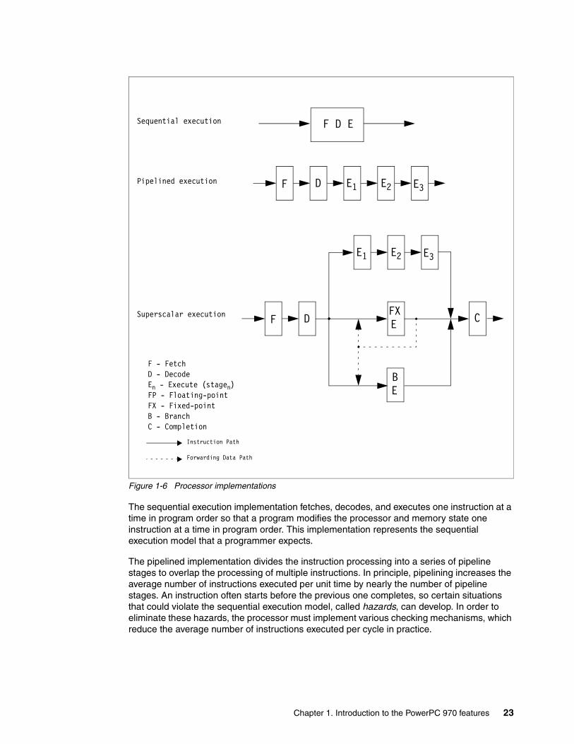
Figure 1-6 Processor implementations

The sequential execution implementation fetches, decodes, and executes one instruction at a time in program order so that a program modifies the processor and memory state one instruction at a time in program order. This implementation represents the sequential execution model that a programmer expects.

The pipelined implementation divides the instruction processing into a series of pipeline stages to overlap the processing of multiple instructions. In principle, pipelining increases the average number of instructions executed per unit time by nearly the number of pipeline stages. An instruction often starts before the previous one completes, so certain situations that could violate the sequential execution model, called hazards, can develop. In order to eliminate these hazards, the processor must implement various checking mechanisms, which reduce the average number of instructions executed per cycle in practice.

Sequential execution F D E

Pipelined execution F D E1 E2 E3

Superscalar execution F D EFX C

E1 E2 E3

EB

Instruction Path

Forwarding Data Path

F - FetchD - DecodeEn - Execute (stagen)FP - Floating-pointFX - Fixed-pointB - BranchC - Completion


The superscalar implementation introduces parallel pipelines in the execution stage to take advantage of instruction parallelism in the instruction sequence. The fetch and decode stages are modified to handle multiple instructions in parallel. A completion stage following the finish of execution updates the processor and memory state in program order. Parallel execution can increase the average number of instructions executed per cycle beyond that possible in a pipelined model, but hazards again reduce the benefits of parallel execution in practice.

The superscalar implementation also illustrates feed-forwarding. The GPR result calculated by a fixed-point operation is forwarded to the input latches of the fixed-point execution stage, where the result is available for a subsequent instruction during update of the GPR.

For fixed-point compares and recording instructions, the CR result is forwarded to the input latches of the branch execution stage, where the result is available for a subsequent conditional branch during the update of the CR.

The PowerPC instruction set architecture has been designed to facilitate pipelined and superscalar (or other parallel) implementations. All PowerPC implementations incorporate multiple execution units and some out-of-order execution capability.

1.8 Application binary interfaceAn application binary interface (ABI) includes a set of conventions that allows a linker to combine separately compiled and assembled elements of a program so that they can be treated as a unit. The ABI defines the binary interfaces between compiled units and the overall layout of application components comprising a single task within an operating system. Therefore, most compilers target an ABI. The requirements and constraints of the ABI relevant to the compiler extend only to the interfaces between shared system elements. For those interfaces totally under the control of the compiler, the compiler writer is free to choose any convention desired, and the proper choice can significantly improve performance.

IBM has defined ABIs for the PowerPC architecture. Other PowerPC users have defined other ABIs. As a practical matter, ABIs tend to be associated with a particular operating system or family of operating systems. Programs compiled for one ABI are frequently incompatible with programs compiled for another ABI because of the low-level strategic decisions required by an ABI. As a framework for the description of ABI issues in this paper, we describe both the AIX ABI for 64-bit systems which uses the Extended Common Object File Format (XCOFF) for object binaries and the PowerOpen™ ABI for 64-bit PowerPC, used by Linux® operating systems that incorporate the Executable and Linking Format (ELF) for object binaries.

At the interface, the ABI defines the use of registers. Registers are classified as dedicated, volatile, or non-volatile. Dedicated registers have assigned uses and generally should not be modified by the compiler. Volatile registers are available for use at all times. Volatile registers are frequently referred to as calling function-save registers. Non-volatile registers are available for use, but they must be saved before being used in the local context and restored prior to return. These registers are frequently referred to as called function-save registers. Table 1-3 on page 25 describes the PowerOpen ABI register conventions for management of specific registers at the procedure call interface.


Table 1-3 PowerOpen ABI register usage convention

Type Register Status Use

General-Purpose Registers

GPR0 Volatile Typically holds return address

GPR1 Dedicated Stack pointer

GPR2 Dedicated Table of contents pointer

GPR3 Volatile First argument word; first word of function return value.

GPR4 Volatile Second argument word; second word of function return value.

GPR5 Volatile Third argument word

GPR6 Volatile Fourth argument word

GPR7 Volatile Fifth argument word

GPR8 Volatile Sixth argument word

GPR9 Volatile Seventh argument word

GPR10 Volatile Eighth argument word

GPR11 Volatile Used in calls by pointer and as an environment pointer

GPR12 Volatile Used for special exception handling and in glink code

GPR 13:31 Non-volatile Values are preserved across procedure calls.


Floating-Point Registers

FPR0 Volatile Scratch register

FPR1 Volatile First floating-point parameter; first floating-point scalar return value.

FPR2 Volatile Second floating-point parameter; second floating-point scalar return value.

FPR3 Volatile Third floating-point parameter; third floating-point scalar return value.

FPR4 Volatile Fourth floating-point parameter; fourth floating-point scalar return value.

FPR5 Volatile Fifth floating-point parameter

FPR6 Volatile Sixth floating-point parameter

FPR7 Volatile Seventh floating-point parameter

FPR8 Volatile Eighth floating-point parameter

FPR9 Volatile Ninth floating-point parameter

FPR10 Volatile Tenth floating-point parameter

FPR11 Volatile Eleventh floating-point parameter

FPR12 Volatile Twelfth floating-point parameter

FPR13 Volatile Thirteenth floating-point parameter

FPR14:31 Non-volatile Values are preserved across procedure calls

Special Purpose Registers

LR Volatile Branch target address; loop count value

CTR Volatile Branch target address; loop count value

XER Volatile Fixed-point exception register

FPSCR Volatile Floating-point status and control register

Condition Register CR0, CR1 Volatile Condition codes

CR2, CR3, CR4

Non-volatile Condition codes

CR5, CR6, CR7

Volatile Condition codes

VMX Registers VR0 Volatile Scratch register

VR1 Volatile Scratch register

VR2 Volatile First vector parameter; return vector data type value

VR3 Volatile Second vector parameter

VR4 Volatile Third vector parameter

VR5 Volatile Fourth vector parameter

VR6 Volatile Fifth vector parameter

VR7 Volatile Sixth vector parameter



Registers GPR1, GPR14 through GPR31, FPR14 through FPR31, VR20 through VR31, and VRSAVE are nonvolatile, which means that they preserve their values across function calls. Functions which use those registers must save the value before changing it, restoring it, and before the function returns. Register GPR2 is technically nonvolatile. However, it is handled specially during function calls as described in the bullet list that follows. In some cases, the calling function must restore its value after a function call.

Registers GPR0, GPR3 through GPR12, FPR0 through FPR13, VR0 through VR19 and the special purpose registers LR, CTR, XER, and FPSCR are volatile, which means that they are not preserved across function calls. Furthermore, registers GPR0, GPR2, GPR11, and GPR12 can be modified by cross-module calls, so a function cannot assume that the values of one of these registers is that which is placed there by the calling function.

The condition code register fields CR0, CR1, CR5, CR6, and CR7 are volatile. The condition code register fields CR2, CR3, and CR4 are nonvolatile. Thus, a function which modifies these fields must save and restore at least those fields of the CR. Languages that require "environment pointers" use GPR11 for that purpose.

The following registers have assigned roles in the standard calling sequence:

� GPR1

Unlike other architectures, there is no stack pointer register. Instead, the stack pointer is stored in GPR1 and maintains quadword alignment. GPR1 always points to the lowest allocated valid stack frame and grows toward low addresses. The contents of the word at that address always point to the previously allocated stack frame. If required, it can be decremented by the called function. The lowest valid stack address is 288 bytes less than the value in the stack pointer. The stack pointer must be atomically updated by a single instruction, thus avoiding any timing window in which an interrupt can occur with a partially updated stack.

� GPR2

ELF processor-specific supplements normally define a Global Offset Table (GOT) section that is used to hold addresses for position-independent code. Some ELF processor-specific supplements, including the 64-bit PowerPC microprocessor supplement, define a small data section. The same register is sometimes used to address both the GOT and the small data section.

The 64-bit PowerOpen ABI defines a Table of Contents (TOC) section. The TOC combines the functions of the GOT and the small data section. This ABI uses the term

VR8 Volatile Seventh vector parameter

VR9 Volatile Eighth vector parameter

VR10 Volatile Ninth vector parameter

VR11 Volatile Tenth vector parameter

VR12 Volatile Eleventh vector parameter

VR13 Volatile Twelfth vector parameter

VR14:19 Volatile Scratch registers

VR20:31 Non-volatile Values are preserved across procedure calls

VRSAVE Non-volatile Contents are preserved across procedure calls



TOC. The TOC section defined here is similar to that defined by the 64-bit PowerOpen ABI. The TOC section contains a conventional ELF GOT, and can optionally contain a small data area. The GOT and the small data area can be intermingled in the TOC section. The TOC section is accessed via the dedicated TOC pointer register, GPR2. Accesses are normally made using the register indirect with immediate index mode supported by the 64-bit PowerPC processor, which limits a single TOC section to 65 536 bytes, enough for 8192 GOT entries.

The value of the TOC pointer register is called the TOC base. The TOC base is typically the first address in the TOC plus 0x8000, thus permitting a full 64 KB TOC. A relocatable object file must have a single TOC section and a single TOC base. However, when the link editor combines relocatable object files to form a single executable or shared object, it can create multiple TOC sections. The link editor is responsible for deciding how to associate TOC sections with object files. Normally the link editor only creates multiple TOC sections if it has more than 65 536 bytes to store in a TOC. All link editors which support this ABI must support a single TOC section, but support for multiple TOC sections is optional. Each shared object has a separate TOC or TOCs.

� GPRs 3:10 (GPR3:10), FPRs 1:13 (FPR1:13), VRs 2:13 (VR2:13)

These sets of volatile registers can be modified across function invocations, and therefore, are presumed by the calling function to be destroyed. They are used for passing parameters to the called function. See 1.10, “Parameter passing” on page 31 for details about passing parameters. In addition, registers GPR3, GPR4 and FPR1 through FPR4 are used to return values from the called function. Example 1-4 on page 29 and Example 1-5 on page 33 illustrate parameter passing and return values.

� Link Register (LR)

This register contains the address to which a called function normally returns. LR is volatile across function calls. The LR can be programmed directly via the mtspr instruction. However, it is typically updated whenever a branch to a subroutine is called. In PowerPC the branch instructions are unconditional branch (bx), conditional branch (bcx), conditional branch to address in CTR register (bcctrx), and conditional branch to address in LR (bclrx). In all four instructions, the x represents two optional parameters. The first option controls whether the address being branched to is relative or absolute. The second option controls whether the LR is updated. Example 1-3 shows the four options for the branch instruction (b).

Example 1-3 Branch instruction options

b 0x500 # This is an unconditional branch to an offset of 0x500 bytes from# the current instruction address.

ba 0x500 # The ‘a’ in the mnemonic indicates a absolute branch to address 0x500.

bl 0x500 # Unconditional branch to offset 0x500 from current instruction# address, ‘l’ in the mnemonic indicates to update LR.

bla 0x500 # Unconditional branch to address 0x500 and update LR.

Note: This ABI does not actually restrict the size of a TOC section. It is permissible to use a larger TOC section, if code uses a different addressing mode to access it. The AIX link editor, in particular, does not support multiple TOC sections, but instead inserts call out code at link time to support larger TOC sections.


Because all PowerPC instructions are four bytes (32 bits), when the letter l is in the mnemonic of the branch type instructions, when the branch is executed, the LR is updated with the address of the current instruction (the branch instruction) plus 4, representing the return address.

GPR3 is an example of a register that performs a dual role. It contains the first positional parameter of the function call and holds the return value when the function returns to the calling function.

Example 1-4 contains the C language code sample.

Example 1-4 Parameter passing

intfoo (int a, char *b, unsigned long c){

int x, y, z;

< body of function >

return (x);}

In the 64-bit PowerPC ABI, when the function foo is called, GPR3 contains the 32-bit signed integer variable a, GPR4 contains the 64-bit pointer to the variable b, and GPR5 contains the 64-bit unsigned variable c. When the function returns back to the calling function, GPR3 contains the value assigned to the 32-bit signed integer variable x.

1.9 The stack frameIn addition to the registers, each function can have a stack frame on the runtime stack. This stack grows downward from high addresses. Figure 1-7 shows the stack frame organization. The symbol “SP” in the figure denotes the stack pointer (GPR1) of the called function after it has executed code establishing its stack frame.

Figure 1-7 Stack frame organization

High Address

Back chainFloating-point register save areaGeneral-purpose register save areaVRSAVE save word (32-bits)Alignment padding (4 or 12 bytes)Vector register save area (quadword aligned)Local variable spaceParameter save area (SP + 48)TOC save area (SP + 40)Link editor doubleword (SP + 32)Compiler doubleword (SP + 24)LR save area (SP + 16)CR save area (SP + 8)Back chain (SP + 0)

Low Address

SP


The following requirements apply to the stack frame:

� The stack pointer maintains quadword alignment.

� The stack pointer points to the first word of the lowest allocated stack frame, the back chain word. The stack grows downward (that is, toward lower addresses). The first word of the stack frame always points to the previously allocated stack frame (toward higher addresses), except for the first stack frame, which has a back chain of 0 (NULL).

� The stack pointer is decremented by the called function in its prologue, if required, and restored prior to return.

� The stack pointer is decremented and the back chain is updated in one operation using the "Store Double Word with Update" instructions, so that the stack pointer always points to the beginning of a linked list of stack frames.

� The sizes of the floating-point and general register save areas can vary within a function and are as determined by the traceback table determined by the number of registers used.

� Before a function changes the value in any nonvolatile FPR, frn, it saves the value in frn in the double word in the FPR save area 8*(32-n) bytes before the back chain word of the previous frame. The FPR save area is always doubleword aligned. The size of the FPR save area depends upon the number of floating point registers which must be saved. It ranges from 0 bytes to a maximum of 144 bytes (18 * 8).

� Before a function changes the value in any nonvolatile general register, rn, it saves the value in rn in the word in the general register save area 8*(32-n) bytes before the low addressed end of the FPR save area. The general register save area is always doubleword aligned. The size of the general register save area depends upon the number of general registers which must be saved. It ranges from 0 bytes to a maximum of 144 bytes (18 * 8).

� Functions must ensure that the appropriate bits in the vrsave register are set for any VRs they use. A function that changes the value of the vrsave register saves the original value of vrsave into the word below the low address end of the general register save area. Below the vrsave area is 4 or 12 bytes of alignment padding, as needed, to ensure that the vrsave area is quadword aligned.

� Before a function changes the value in any nonvolatile VR, VRn, it saves the value in VRn in the vrsave area 16*(32-n) bytes before the low addressed end of the vrsave area plus alignment padding. The vrsave area is always quadword aligned. The size of the vrsave area depends upon the number of VRs which must be saved; it ranges from 0 bytes to a maximum of 192 bytes (12 * 16).

� The local variable space contains any local variable storage required by the function. If VRs are saved the local variable space area is padded so that the vrsave area is quadword aligned.

� The parameter save area is allocated by the calling function. It is doubleword aligned, and is at least eight doublewords in length. If a function needs to pass more than eight doublewords of arguments, the parameter save area is large enough to contain the arguments that the calling function stores in it. Its contents are not preserved across function calls.

� The TOC save area is used by global linkage code to save the TOC pointer register.

� The link editor doubleword is reserved for use by code generated by the link editor. This ABI does not specify any usage. The AIX link editor uses this space under certain circumstances.

� The compiler doubleword is reserved for use by the compiler. This ABI does not specify any usage; the AIX compiler uses this space under certain circumstances.


� Before a function calls any other functions, it saves the value in the LR register in the LR save area.

� Before a function changes the value in any nonvolatile field in the CR, it saves the values in all the nonvolatile fields of the CR at the time of entry to the function in the CR save area.

� The 288 bytes below the stack pointer is available as volatile storage which is not preserved across function calls. Interrupt handlers and any other functions that might run without an explicit call must take care to preserve this region. If a function does not need more stack space than is available in this area, it does not need to have a stack frame.

The stack frame header consists of the back chain word, the CR save area, the LR save area, the compiler and link editor doublewords, and the TOC save area, for a total of 48 bytes. The back chain word always contains a pointer to the previously allocated stack frame. Before a function calls another function, it saves the contents of the link register at the time that the function was entered in the LR save area of its calling function's stack frame and establishes its own stack frame.

Except for the stack frame header and any padding necessary to make the entire frame a multiple of 16 bytes in length, a function need not allocate space for the areas that it does not use. If a function does not call any other functions and does not require any of the other parts of the stack frame, it need not establish a stack frame. Any padding of the frame as a whole is within the local variable area. The parameter save area immediately follows the stack frame header, and the register save areas contains no padding except as noted for VR save.

1.10 Parameter passingFor 64-bit PowerPC microprocessors like the PowerPC 970, it is generally more efficient to pass arguments to called functions in registers (general-purpose, floating-point, and VRs) than to construct an argument list in storage or to push them onto a stack. Because all computations must be performed in registers anyway, memory traffic can be eliminated if the calling function can compute arguments into registers and pass them in the same registers to the called function, where the called function can then use them for further computation in the same registers. The number of registers implemented in a processor architecture naturally limits the number of arguments that can be passed in this manner.

For the 64-bit PowerPC 970, up to eight doublewords are passed in GPRs, that are loaded sequentially into GPR3 through GPR10. Up to 13 floating-point arguments can be passed in FPRs FPR1 through FPR13. If VMX is used, up to 12 vector parameters can be passed in VR2 through VR13. If fewer (or no) arguments are passed, the unneeded registers are not loaded and contains undefined values on entry to the called function.

The parameter save area, which is located at a fixed offset of 48 bytes from the stack pointer, is reserved in each stack frame for use as an argument list. A minimum of eight doublewords is always reserved. The size of this area must be sufficient to hold the longest argument list that is passed by the function which owns the stack frame. Although not all arguments for a particular call are located in storage, they form a list in this area, with each argument occupying one or more doublewords.

If more arguments are passed than can be stored in registers, the remaining arguments are stored in the parameter save area. The values passed on the stack are identical to those that have been placed in registers. Thus, the stack contains register images.

For variable argument lists, this ABI uses a va_list type which is a pointer to the memory location of the next parameter. Using a simple va_list type means that variable arguments


must always be in the same location regardless of type, so that they can be found at runtime. This ABI defines the location to be general registers GPR3 through GPR10 for the first eight doublewords and the stack parameter save area thereafter. Alignment requirements such as those for vector types can require the va_list pointer to first be aligned before accessing a value.

The rules for parameter passing are as follows:

1. Each argument is mapped to as many doublewords of the parameter save area as are required to hold its value.

a. Single-precision floating point values are mapped to the first word in a single doubleword.

b. Double-precision floating point values are mapped to a single doubleword.

c. Extended-precision floating point values are mapped to two consecutive doublewords.

d. Simple integer types (char, short, int, long, enum) are mapped to a single doubleword. Values shorter than a doubleword are sign- or zero-extended as necessary.

e. Complex floating point and complex integer types are mapped as though the argument was specified as separate real and imaginary parts.

f. Pointers are mapped to a single doubleword.

g. Vectors are mapped to a single quadword, quadword aligned. This can result in skipped doublewords in the parameter save area.

h. Fixed size aggregates and unions passed by value are mapped to as many doublewords of the parameter save area as the value uses in memory. Aggregrates and unions are aligned according to their alignment requirements. This can result in doublewords being skipped for alignment.

i. An aggregate or union smaller than one doubleword in size is padded so that it appears in the least significant bits of the doubleword. All others are padded, if necessary, at their tail. Variable size aggregates or unions are passed by reference.

j. Other scalar values are mapped to the number of doublewords required by their size.

2. If the called function has a known prototype, arguments are converted to the type of the corresponding parameter before being mapped into the parameter save area. For example, if a long is used as an argument to a float double parameter, the value is converted to double-precision and mapped to a doubleword in the parameter save area.

3. Floating point registers FPR1 through FPR13 are used consecutively to pass up to 13 single, double, and extended-precision floating point values and to pass the corresponding complex floating point values. The first 13 of all doublewords in the parameter save area that map floating point arguments, except for arguments corresponding to the variable argument part of a called function with a prototype containing an ellipsis, are passed in floating point registers. A single-precision value occupies one register as does a double-precision value. Extended-precision values occupy two consecutively numbered registers. The corresponding complex values occupy twice as many registers.

4. VR2 through VR13 are used to consecutively pass up to 12 vector values, except for arguments corresponding to the variable argument part of a called function with a prototype containing an ellipsis.

5. If there is no known function prototype for a called function, or if the function prototype for a called function contains an ellipsis and the argument value is not part of the fixed arguments described by the prototype, then floating point and vector values are passed according to the ABI specification for non-floating, non-vector types. In the case of no known prototype, two copies of floating and vector argument values being passed.


6. GPRs are used to pass some values. The first eight doublewords mapped to the parameter save area correspond to the registers GPR3 through GPR10. An argument other than floating point and vector values fully described by a prototype, that maps to this area either fully or partially, is passed in the corresponding general registers.

7. All other arguments (or parts thereof) not already covered must be stored in the parameter save area following the first eight doublewords. The first eight doublewords that are mapped to the parameter save area are never stored in the parameter save area by the calling function.

8. If the called function takes the address of any of its parameters, then values passed in registers are stored into the parameter save area by the called function. If the compilation unit for the calling function contains a function prototype, but the called function has a mismatching definition, this can result in the wrong values being stored.

Example 1-5 illustrates an example of parameter passing.

Example 1-5 Parameter passing example

typedef struct {int s1;double s2;

} s_param;

s_param a, b;int c, d, e, f;long double g;double h, i, j;

f = func (c, h, d, g, a, i, b, e, j);

Parameter Register Offset Stored in parameter save area?c GPR3 0-7 Noh FPR1 8-15 Nod GPR5 16-23 Nog FPR2,FPR3 24-39 Noa GPR8,GPR9 40-55 Noi FPR4 56-63 Nob (none) 64-79 Yese (none) 80-87 Yesj FPR5 88-95 No

1.11 Return valuesFunctions return float or double values in FPR1, with float values rounded to single precision. When the VMX facility is used, functions return vector data type values in VR2. Functions return values of type int, long, enum, short, and char, or a pointer to any type, as unsigned or signed integers as appropriate, zero- or sign-extended to 64 bits if necessary, in GPR3. Character arrays of length eight bytes or less, or bit strings of length 64 bits or less, are returned right justified in GPR3. Aggregates or unions of any length and character strings of length longer than eight bytes are returned in a storage buffer allocated by the calling function. The calling function passes the address of this buffer as a hidden first argument in GPR3, causing the first explicit argument to be passed in GPR4. This hidden argument is treated as a normal formal parameter and corresponds to the first doubleword of the parameter save area.


Functions return floating point scalar values of size 16 or 32 bytes in FPR1:FPR2 and FPR1:FPR4, respectively.

Functions return floating point complex values of size 16 (four or eight byte complex) in FPR1:FPR2 and floating point complex values of size 32 (16 byte complex) in FPR1:FPR4.

1.12 SummaryThis chapter reviewed the basics of the PowerPC 64-bit architecture and described briefly the programming environment. You can find a more detailed discussion of this material in other Redpapers, Redbooks, and documents available from IBM at:

ibm.com/redbooks

The focus of this paper now turns to describing the performance advantages of the VMX engine found in the PowerPC 970.




Chapter 2. VMX in the PowerPC 970

This chapter covers the details of the VMX execution unit. It contains a general overview of vectorization as well as a review of vector terminology. In addition, this chapter also includes information about vector memory addressing and instruction categories.

For detailed information about these topics, see PowerPC Microprocessor Family: AltiVec Technology Programming Environments. For information about this and other documentation that is available, see “Related publications” on page 119.

2


2.1 Vectorization overviewSo why should you care about vector technology? The answer is simple, performance! Vector technology can provide dramatic performance gains. The best way to understand how vectorization can improve performance is to look first at the instruction level.

Consider a simple scalar vector addition as shown in Example 2-1. In this example, the scalar addition a[i] = b[i] + c[i], is performed in a single cycle.

Example 2-1 Scalar vector addition

for ( i = 0, i++, i < n){ a[i] = b[i] + c[i]; // scalar version}

Next consider a vectorized version of the same loop as shown in Example 2-2.

Example 2-2 Vectorization of scalar addition

for ( i = 0, i++, i < n / vector_size) { a[i] = vec_add(b[i] , c[i]); // vectorized version}

In Example 2-2, while not shown explicitly, the scalar data type has been replaced by vector data types. Note that the loop range no longer n but is reduced by vector_size. Remember that the size of a vector register (VR) is 128 bits. Therefore, the vector addition operation, a[i] = vec_add(b[i],c[i]), can execute in a single clock cycle for each vector, as opposed to many clock cycles using multiple scalar instructions.Thus, the vectorized version executes vector_size times faster.

Given the various data types for the 128-bit VRs, the following performance gains using a single functional unit are possible:

� For an 8-bit integer, vector_size = 16 yields a 16x performance gain� For an 16-bit integer, vector_size = 8 yields a 8x performance gain� For an 32-bit integer, vector_size = 4 yields a 4x performance gain� For an 32-bit float, vector_size = 4 yields a 4x performance gain

Because the PowerPC 970 has two scalar floating-point units and one vector floating-point unit, the actual peak performance for 32-bit floating point arithmetic may only provide a 2x performance gain compared to scalar code that can keep both floating point units busy.

These performance gains should be considered as upper bounds. Performance is limited by how well the application can keep the vector unit busy as well as cache and memory considerations.

The vector technology provides a software model that accelerates the performance of various software applications and extends the instruction set architecture (ISA) of the PowerPC architecture. The instruction set is based on separate vector/SIMD-style (single instruction stream, multiple data streams) execution units that have high data parallelism. This high data parallelism can perform operations on multiple data elements in a single instruction.

The term vector in this paper refers to the spatial parallel processing of short, fixed-length one-dimensional matrixes performed by an execution unit. It should not be confused with the temporal parallel (pipelined) processing of long, variable length vectors performed by classical vector machines. High degrees of parallelism are achievable with simple in-order


instruction dispatch and low-instruction bandwidth. However, the ISA is designed so as not to impede additional parallelism through superscalar dispatch to multiple execution units or multithreaded execution unit pipelines.

Vector technology in the PowerPC 970 supports the following audio and visual applications:

� Voice over IP (VoIP)

– VoIP transmits voice as compressed digital data packets over the internet.

� Access Concentrators/DSLAMS

– A DSLAM is a network device, usually at a telephone company central office, that receives signals from multiple Digital Subscriber Line (DSL) connections and places the signals on the internet.

� Speech recognition

– Speech processing allows voice recognition for use in applications like directory assistance and automatic dialing.

� Voice/Sound Processing (audio decode and encode): G.711, G.721, G.723, G,729A, and AC-3

– Voice processing is used to improve sound quality on lines.

� Communications

– Multi-channel modems

– Software modem: V.34, 56 K

– Data encryption: RSA

– Basestation processing: cellular basestation compresses digital voice data for transmission within the internet.

– High bandwidth data communication

– Modem banks can use the vector technology to replace signal processors in DSP farms.

– Echo cancellation: The echo cancellation is used to eliminate echo build up on long landline calls.

� 2D and 3D graphics.

– Such as QuickDraw, OpenGL, VRML, Games, Entertainment, and High-precision CAD

� Virtual reality

� High-fidelity audio

– 3D audio, AC-3. Hi-Fi Audio uses VMX’s FPU.

� Image and video processing

– JPEG, filters

– Motion video decode and encode: MPEG-1, MPEG-2, MPEG-4, and H.234

– Video conferencing: H.261, H.263

� Array number processing

� Real-time continuous speech I/O: HMM, Viterbi acceleration, Neural algorithms

� Machine Intelligence

Chapter 2. VMX in the PowerPC 970 37

In summary, vector technology found in the PowerPC 970 defines the following:

� Fixed 128-bit wide vector length that can be subdivided into sixteen 8-bit bytes, eight 16-bit half words, or four 32-bit words.

� VR file architecturally separate from floating-point registers (FPRs) and general-purpose register (GPRs).

� Vector integer and floating-point arithmetic.

� Four operands for most instructions (three source operands and one result).

� Saturation clamping.

– Where unsigned results are clamped to zero on underflow and to the maximum positive integer value (2n-1, for example, 255 for byte fields) on overflow. For signed results, saturation clamps results to the smallest representable negative number (-2n-1, for example, -128 for byte fields) on underflow, and to the largest representable positive number (2n-1-1, for example, +127 for byte fields) on overflow).

� No mode switching that would increase the overhead of using the instructions.

� Operations selected based on utility to digital signal processing algorithms (including 3D).

� Vector instructions provide a vector compare and select mechanism to implement conditional execution as the preferred way to control data flow in vector programs.

� Enhanced cache and memory interface.

2.1.1 Vector technology reviewVector technology expands the PowerPC architecture through the addition of a 128-bit vector execution unit, which operates concurrently with the existing integer- and floating-point units. This new engine provides for highly parallel operations, allowing for the simultaneous execution of up to four 32-bit floating operations or sixteen 8-bit fixed-point operations in one instruction. All VPU datapaths and execution units are 128 bits wide and are fully pipelined..

This technology can be thought of as a set of registers and execution units that can be added to the PowerPC architecture in a manner analogous to the addition of floating-point units. Floating-point units were added to provide support for high-precision scientific calculations and the vector technology is added to the PowerPC architecture to accelerate the next level of performance-driven, high-bandwidth communications and computing applications. (Figure 2-1 on page 39 provides the high level structural overview of the PowerPC 970 with vector technology.)


Figure 2-1 High level structural overview of PowerPC 970

This paper frequently uses the families of terms that are derived from vectorization and autoSIMDization. Because these terms can be used differently, it is necessary to highlight their meanings. The term vectorization has traditionally been referred to as the processing of vectors (arrays) of any length. Automatic vectorization is when a compiler recognizes and exploits opportunities to substitute vector instructions in scalar code.

When short-vector processing was added as a feature to microprocessors, the enhancements were referred to as SIMD instructions to distinguish them as a subclass of the more general vector hardware. Thus, autoSIMDization refers to a compiler that translates scalar code to specifically generate these short vector instructions. These vector instructions make up the set for PowerPC computers.

This document uses the term vectorization as applied to short vectors with VMX instructions.

The key features of the PowerPC 970 implementation include:

� All datapaths and execution units are 128-bits wide

� Two independent vector processing sub-units, one for all arithmetic logic unit (ALU) instructions and one for permute operations

Vector instructions can be freely intermixed with existing PowerPC instructions to form a complete program. Vector instructions provide a vector compare and select mechanism to implement conditional execution as the preferred mechanism to control data flow in vector programs. In addition, vector compare instructions can update the condition register, thus providing the communication from the vector processing unit to the PowerPC branch instructions necessary to modify program flow based on vector data.

The vector processing unit is divided into two dispatchable units: vector ALU and vector Permute. The vector ALU unit is further subdivided into a vector floating-point unit, a vector simple-fixed unit, and a vector complex-fixed unit. The vector ALU and permute units receive predecoded instructions via the Issue Queue in the Instruction Sequencer Unit for the VPU (ISV). Vector instructions are issued to the appropriate vector unit when all of the source

InstructionFetch

DispatchReg. Mapping

FXU1 FXU2 VMXPermute

VMXALU

FPU1 FPU2

General-PurposeRegisters

VectorRegisters

Floating-PointRegisters

Vector Unit

VectorRegisters


operands are available. Vector loads, stores, or dsts instructions are executed in the LSU pipes. There are two copies of the VR files. One provides operands for the vector permute unit, and one provides operands for the vector ALU.

The vector technology is purposefully simple such that there are no exceptions other than DSI exceptions on loads and stores, no hardware unaligned access support, and no complex functions. The vector technology is scaled down to only the necessary pieces in order to facilitate efficient cycle time, latency, and throughput on hardware implementations.

In the vector execution unit, the ALU operates on from one to three source vectors and produces a single result/destination vector on each instruction. The ALU is an SIMD-style arithmetic unit that performs the same operation on all the data elements that comprise each vector. This scheme allows efficient code scheduling in a highly parallel processor. Load and store instructions are the only instructions that transfer data between registers and memory. Figure 2-2 shows the vector unit and VR file. This SIMD-style execution unit executes instructions that perform operations in parallel on the data elements that comprise each vector. Architecturally, the VR file is separate from the GPRs and FPRs.

Figure 2-2 VMX top-level diagram

VR0

VR1

VR2

VR3

VR31

VR30

Result/Destination Vector Register

128 128 128

128

Vector Register File (VRF)

Vector Execution Unit


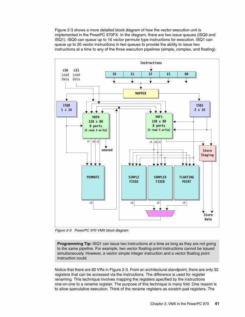
Figure 2-3 shows a more detailed block diagram of how the vector execution unit is implemented in the PowePC 970FX. In the diagram, there are two issue queues (ISQ0 and ISQ1). ISQ0 can queue up to 16 vector permute type instructions for execution. ISQ1 can queue up to 20 vector instructions in two queues to provide the ability to issue two instructions at a time to any of the three execution pipelines (simple, complex, and floating).

Figure 2-3 PowerPC 970 VMX block diagram

Notice that there are 80 VRs in Figure 2-3. From an architectural standpoint, there are only 32 registers that can be accessed via the instructions. The difference is used for register renaming. This technique involves mapping the registers specified by the instructions one-on-one to a rename register. The purpose of this technique is many fold. One reason is to allow speculative execution. Think of the rename registers as scratch-pad registers. The

Programming Tip: ISQ1 can issue two instructions at a time as long as they are not going to the same pipeline. For example, two vector floating-point instructions cannot be issued simultaneously. However, a vector simple integer instruction and a vector floating point instruction could.

vDvDvD

vA vB vCvCvBvA

I0 I1 I2 I3 BR

Instructions

MAPPER

ISQ01 x 16

ISQ12 x 10

VRF0128 x 808 ports

(4 read 4 write)

VRF1128 x 808 ports

(4 read 4 write)

LS0LoadData

LS1LoadData

PERMUTE

unused

SIMPLEFIXED

COMPLEXFIXED

FLOATINGPOINT

StoreStaging

StoreData

vD


result of the operation is temporarily stored in the rename register. If the instruction is on a valid execution path (no outstanding branch conditions), then during the completion stage of the pipeline and in program order, the contents are copied to the specified destination (target) register, vD of the instruction.

Another purpose of the rename registers is for out-of-order execution of instructions in the superscalar design of a PowerPC 970. If an interrupt or exception occurs, some instructions will have already finished execution. However, they cannot write their results back to the architected register because doing so would be out of program order. This condition might be because another instruction is currently stalled waiting on an operand from memory such as a load. If an exception occurs on the load due to illegal addressing, permission, and son on, then the state of the machine has to reflect what the processor state would be in a sequential execution model. The architected registers need to contain the values at the time of the exception, not what they could be had the instruction not caused an exception. The results in the rename registers for those instructions that come after the exception-causing instruction in the program, have their results, if finished, discarded. To assure proper processor state, all instruction prior to the exception-causing instruction have results copied from the rename register to the specified architected register before the exception is handled by the processor.

2.2 Vector memory addressingVectors are accessed from memory with instructions such as Load Vector Indexed (lvx) and Store Vector Indexed (stvx). The operand of a VR to memory access instruction has a natural alignment boundary equal to the operand length. In other words, the natural address of an operand is an integral multiple of the operand length. A memory operand is said to be aligned if it is aligned at its natural boundary; otherwise, it is misaligned. As with all PowerPC instructions, vector instructions are 32-bit words and on word boundaries.

Table 2-1 shows the characteristics for operands for VR to memory access instructions.

Table 2-1 Memory operand alignment

A vector is 128 bit (16 bytes) and needs to be aligned on 16 byte boundaries. For example, the load vector indexed instruction takes the contents of GPR A and the contents of GPR B and then ANDs the value with ~0xF to form the effective address to load the vector from, as shown in the following example:

lvx vD, rA, rB

Note that ANDing with ~0xF forces the scalar to be on quadword boundaries.

Operand Length Aligned address (28:31)a

a. An x in an address bit position indicates that the bit can be 0 or 1 independent of the state ofother bits in the address.

Byte 8 bits (1 byte) xxxx

Halfword 16 bits (2 bytes) xxx0

Word 32 bits (4 bytes) xx00

Quadword 128 bits (16 bytes) 0000


malloc() versus vec_malloc()The memory allocation functions supplied through the C standard library are not required to return a vector aligned address. The vector standard specifies additional functions such as vec_malloc() and vec_free(), which do return a properly aligned address for vector operations. Neither gcc or xlc support these functions at this time. The xmalloc() kernel routine in AIX does allow the kernel programmer to specify the starting address boundary. For example, the following would return an address where the least significant four address bits are zero, resulting in a quadword aligned data area:

char *ptr = xmalloc(size, 4, kernel_heap);

For non-AIX kernel programmers, you could perform a malloc plus 16 additional bytes (128 bits), then AND the returned address with ~0xF to assure quadword alignment. An example of this code is available in the testVMX software suite developed by the CEPBA-IBM Research Institute and distributed under the GNU General Public License. Due to policy constraints, we cannot show the code in this paper. You can view the code at:

http://www.ciri.upc.es/cela_pblade/testVMX.htm

Another technique for assuring proper alignment is using the alignx or __alignx xlc compiler builtins as described in “The alignx builtin” on page 73.

Cache management instructionsFor those assembly language programmers who want to get a little more performance out of your vector application, consider the vector cache management instructions dst, dstst, dss, and dssall.

The central idea here is to reduce the latency of accessing memory using the vector load and store instructions. If the load instruction is executed and the vector being accessed is not currently in the cache, a delay occurs waiting for the data to come from memory. The delay is based upon the bus frequency and other factors such as type of memory, current bus traffic, and so on. The dst and dstst instructions are instructions designed to prefetch data into the cache because the program will soon load and store data, respectively. Think of it as a background operation preloading the cache in parallel with current executing instructions. When the program gets to the point where it starts processing the data, the load and store operations hit the cache.

The data stream touch instruction can be specified as either dst or dstt. The extra t at the end of the mnemonic indicates that the T bit is to be set in the instruction. Setting the T bit indicates to the processor that this data being touched into the cache is transient. As the term implies, transient means that the data is “just passing through” and the program is likely not to reference it again. When the cache becomes saturated, transient data is replaced before non-transient data. The PowerPC 970 does not support the concept of transient data, and this bit is ignored. It is mentioned here because future processors may support this feature. Currently, the PowerPC 440 embedded controllers are examples of PowerPC implementations that support transient data.

Programming Note: For the lvx instruction, if rA is zero, it does not use the contents of GPR 0 simply 0 is added to the contents of rB. This characteristic is found in other PowerPC instructions as well. Some disassemblers incorrectly format this type of instruction. For example, they may display lvx v3, r0, r5, when instead they should display lvx v3, 0, r5.


http://www.ciri.upc.es/cela_pblade/testVMX.htm

The syntax of the data stream touch instructions is:

dst rA, rB, STRM (T = don’t care)

GPR A contains the 64-bit starting effective address of the data area to be touched in. GPR B contains the block size, block count, and block stride values. The format of GPR B is shown in Figure 2-4.

Figure 2-4 Cache prefetch control

The STRM field in the dst instruction is a two-bit field that indicates which of the four prefetch streams to use for prefetching blocks of vectors. This field represents that it is possible to be prefetching data into the caches from four separate data areas.

Note that bits 0:31 of GPR B are reserved and not shown in Figure 2-4. Bits 32:34 are also reserved. Bits 35:39 represent the size of the block in vectors. Because this is a five bit field, the programmer can specify that a block is 32 vectors (25 = 32) or 512 bytes (32 vectors times 16 bytes per vector). A block size value of all zeros for bits 35:39 indicates a block size of 32 vectors. Any other bit values represent the number of vectors that make up the block size.

The block count field is a 8-bit field and is used by the programmer to specify the number of blocks to prefetch. A block count of zero (0) indicates 256 blocks while any other value for this field indicates the number of blocks to prefetch.

The block stride is a signed offset to the next block in bytes and can be negative. This 16-bit field provides an offset range of -32,768 to +32,768. A value of zero (0) for this field indicates an offset of +32,768 bytes. Any other value for this field represent the offset to the next block.

Reserved Block size Block count Signed block stride

32 34 35 39 40 47 48 63

Block 0 Block 1 Block 2 Block 3

System Memory

Stream

Block size = (rB)35:39

Block stride = (rB)48:63

Format of GPR B (bits 0:31 reserved)

Starting address = (rA)

Important: Do not confuse the term block used here with the term cache block used in PowerPC. In the PowerPC 970 a cache block or line is fixed at 128 bytes.


PowerPC 970 vector prefetch implementationFor the PowerPC 970, there are eight hardware prefetch streams and they are divided into two groups of four prefetch streams. Four of these are used for the vector prefetch instructions and support vector style prefetching, with some restrictions.

Relatively simple mapping hardware is used to convert the dst instruction request into an asynchronous prefetch of n-cache lines into the caches. The first line is placed into the L1 cache, and the remaining lines are placed in the L2 cache. However, due to the nature of the dst instructions and the available data and control paths in PowerPC 970, these instructions are not executed speculatively. Speculative execution means that the execution path of instructions might not be valid. For example, in PowerPC when a conditional branch is executed, the condition on whether the branch is to be taken might not be known. This condition can be caused by an instruction that updates the CR during its execution and that is perhaps stalled while waiting on a dependency to be fulfilled.

Consider the code fragment in Example 2-3.

Example 2-3 Speculative execution

lwz r4, 32(r5) # Load miss on caches, needs to go to memorycmpwi CR0, r4, 0 # Compare loaded value to zero, set CR0 to indicate less than,

# greater than, or equal tobeq my_sub # If equal bit is set, branch to the subroutine, my_sub

Keeping in mind the execution pipelines shown in Figure 1-1 on page 8, the lwz instruction would go to either LS1 or LS2 , the cmpwi would go to the CR pipeline, and the beq would go to the BR pipeline — all at the same time. Because the load misses the cache, the cmpwi instruction has to wait longer for the value to compare to. The conditional branch instruction (beq), however, is not going to wait. It is going to take its best guess. This guess can be based on previous branch history in the Branch History Table or, if no entry in the table is present, can use the 90:10 rule. (The 90:10 rule states that, in general, 90 percent of a program’s execution time is only spent in 10 percent of its code due to looping.)

Looping in code is a branch in the negative direction with respect to program flow. Therefore, in all PowerPC implementations, when the processor encounters a conditional branch instruction with a negative displacement and when there is no history recorded for this branch instruction, the branch is predicted to be taken, and the fetching of the instructions is performed. Conditional branch instructions that have a positive or forward displacement are predicted not to be taken and the next sequential instructions are fetched. The execution of the speculative fetched instructions is called speculative execution. Therefore, in Example 2-3, if the branch to my_sub is predicted to be taken, and it attempts to execute a dst instruction, the dst instruction will stall until the outcome of cmpwi is known and the execution path validated.

In the case where the block count is not one (1), there are three cases where the number of lines prefetched are based on the stride. These are:

� Block stride equals block size� Block stride is 128 bytes� Block stride is less than 128 bytes

Storing to streams (dstst instruction)A dst instruction brings a cache block into the cache subsystem in a state most efficient for subsequent reading of data from it (load). The companion instruction, Data Stream Touch for Store (dstst), brings the cache block into the cache subsystem in a state most efficient for subsequent writing to it (store). For example, in a modified, exclusive, shared and invalid cache subsystem, a dst might bring a cache block in shared (S) state, while a dstst would


bring the cache block in exclusive (E) state to avoid a subsequent demand-driven bus transaction to take ownership of the cache block so the store can proceed due to sharing with another processor. The PowerPC 970 does not implement this feature and treats the dstst instruction as a dst instruction.

Stopping streams (dss instructions)The dst instructions have a counterpart called Data Stream Stop (dss). A program can stop any given stream prefetch by executing dss with that stream’s tag. This is useful when a program speculatively starts a stream prefetch but later determines that the data no longer needs to be processed due to an error. The dss instruction can stop the stream so that no more bandwidth is wasted. All active streams can be stopped by using dssall. This option is useful when the operating system needs to stop all active streams (context switch) but does not know how many streams are in progress.

Because dssall does not specify the number of implemented streams, it should always be used instead of a sequence of dss instructions to stop all streams.

Neither dss nor dssall is execution synchronizing. The time between when a dss is issued and when the stream stops is not specified. Therefore, when the software must ensure that the stream is physically stopped before continuing (for example, before changing virtual memory mapping), a special sequence of synchronizing instructions is required. The sequence can differ for different situations, but the sequence shown in Example 2-4 works in all contexts.

Example 2-4 Stopping prefetch streams

dssall # stop all streamssync # insert a barrier in memory pipe

loop: lwz Rx, 0(Ry) # stick one more operation in memory pipecmpd Rn, Rnbne loop # make sure load data is backisync # wait for all previous instructions to complete to

# ensure memory pipe is clear and nothing is pending# in the old context

PowerPC 970 implementation restrictionsThe following restrictions are found in the PowerPC 970 microprocessor:

� All dst instructions, including the stop instructions, are non-speculative.

� The instruction dstst is supported as a dst only.

� The dst instructions are terminated at a page boundary (no page crossing).

� Optionally, alignment may be handled by prefetching one line past the dst end.

� The transient hint is ignored.

� There is no monitoring of the MSR[PR] bit by the prefetch hardware.

� The prefetch hardware suspends dst operations when MSR[DR] is set to zero (0).

� Negative stride cases where the block size is greater than 128 bytes result in incorrect prefetching of the first block. The mapping hardware fetches one line of the block and then begins the negative direction accesses.

� Total number of outstanding prefetch requests active as a result of dst instructions are limited to four.

� The mapping hardware assumes strides are a power of two.

� An enable/disable for data prefetch is located in the HID4[25].


� An enable for vector prefetch support is located in HID5[54:55]. These bits are set to b‘00’ to enable the use of four of the hardware prefetch streams as vector streams. If set to b‘11’, all eight streams are used as hardware prefetch streams, and all vector prefetch instructions are treated as no-ops by the load and store unit’s prefetch hardware.

In summary, it might be worth the effort to implement stream prefetching in the application to boost performance. For further details consult the IBM PowerPC 970FX RISC Microprocessor User’s Manual. For information about this and other documentation that is available, see “Related publications” on page 119.Saturation detection (overflow and underflow)

Most integer instructions have both signed and unsigned versions and many have both modulo (wrap-around) and saturating clamping modes. Saturation occurs whenever the result of a saturating instruction exceeds the maximum or minimum value for that data type. For example, for an unsigned integer, a negative result (underflow) will trigger a saturation condition. There is hardware support for detecting this arithmetic condition, and there is no performance penalty for the correction. The action taken is to clamp underflows to the minimum value in the data type’s range and overflows to the maximum value in the data type’s range, as opposed to generating not-a-number or machine infinity or a program-terminating error condition.

Saturation conditions can be set by the following types of integer, floating-point, and formatting instructions:

� Move to VSCR (mtvscr)

� Vector add integer with saturation (vaddubs, vadduhs, vadduws, vaddsbs, vaddshs, vaddsws)

� Vector subtract integer with saturation (vsububs, vsubuhs, vsubuws, vsubsbs,vsubshs, vsubsws)

� Vector multiply-add integer with saturation (vmhaddshs, vmhraddshs)

� Vector multiply-sum with saturation (vmsumuhs, vmsumshs, vsumsws)

� Vector sum-across with saturation (vsumsws, vsum2sws, vsum4sbs, vsum4shs, vsum4ubs)

� Vector pack with saturation (vpkuhus, vpkuwus, vpkshus, vpkswus, vpkshss, vpkswss)

� Vector convert to fixed-point with saturation (vctuxs, vctsxs)

Integer instructions in modulo mode and floating-point arithmetic instructions never trigger a saturation condition.

2.3 Instruction categoriesAs with PowerPC instructions, vector instructions are encoded as single-word (32-bit) instructions. Instruction formats are consistent among all instruction types, permitting decoding to be parallel with operand accesses. This fixed instruction length and consistent format simplifies instruction pipelines. vector load, store, and stream prefetch instructions have the primary opcode of 31 (0b011111) and use an extended opcode to differentiate the instructions (see 1.6, “PowerPC instructions” on page 19 for a description of extended opcodes). Vector ALU-type instructions use a primary opcode of 4 (0b000100).

The vectorization engine supports both intraelement and interelement operations.

� intraelement operations

Elements work in parallel on the corresponding elements from multiple source operand registers and place the results in the corresponding fields in the destination operand


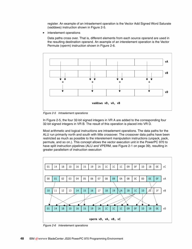
register. An example of an intraelement operation is the Vector Add Signed Word Saturate (vaddsws) instruction shown in Figure 2-5.

� interelement operations

Data paths cross over. That is, different elements from each source operand are used in the resulting destination operand. An example of an interelement operation is the Vector Permute (vperm) instruction shown in Figure 2-6.

Figure 2-5 Intraelement operations

In Figure 2-5, the four 32-bit signed integers in VR A are added to the corresponding four 32-bit signed integers in VR B. The result of this operation is placed into VR D.

Most arithmetic and logical instructions are intraelement operations. The data paths for the ALU run primarily north and south with little crossover. The crossover data paths have been restricted as much as possible to the interelement manipulation instructions (unpack, pack, permute, and so on.). This concept allows the vector execution unit in the PowerPC 970 to have split instruction pipelines (ALU and VPERM, see Figure 2-1 on page 39), resulting in greater parallelism of instruction execution

Figure 2-6 Interelement operations

+ + + +

vaddsws vD, vA, vB

vD

vB

vA

vperm vD, vA, vB, vC

01 14 18 10 16 15 19 1A 1C 1C 1C 09 0F 1D 1B 0E vC

00 01 02 03 04 05 06 07 08 09 0A 0B 0C 0D 0E 0F vA

10 11 12 13 14 15 16 17 18 19 1A 1B 1C 1D 1E 1F vB

01 14 18 10 16 15 19 1A 1C 1C 1C 09 0F 1D 1B 0E vD


In Figure 2-6 on page 48, vperm allows any byte under the control of vC in two source registers (vA and vB) to be copied into a destination register (vD). Specifically, the vperm instruction takes the contents of vA and concatenates the contents of vB forming a 32 byte (0 to 1F) temporary value. Based on the value stored in each one of the 16 8-bit fields of vC, the corresponding byte of the temporary value is copied into the corresponding 8-bit field of vD. In our example, the resulting value that is placed into vD has the same value as vC because the data stored in vA and vB was generated to show the 32 bytes (0 to 1F) for clarification purposes. For example, the left-most 8-bits of vC has the value 0f 0x01. From the temporary value of 32 bytes, take byte 0x01 and place it into the left-most eight bits (0:7) of vD. The next eight bits of vC contains the value 0x14. From the 32-byte temporary value, place the value of byte 20 (0x14) into the next eight bits (8:15) of vD.

We can break down the vector instructions as follows:

� Vector intraelement instructions

– Vector integer instructions

• Vector integer arithmetic instructions• Vector integer compare instructions• Vector integer rotate and shift instructions

– Vector floating-point instructions

• Vector floating-point arithmetic instructions• Vector floating-point rounding and conversion instructions• Vector floating-point compare instruction• Vector floating-point estimate instructions

– Vector memory access instructions

� Vector interelement instructions

– Vector alignment support instructions

– Vector permutation and formatting instructions

• Vector pack instructions• Vector unpack instructions• Vector merge instructions• Vector splat instructions• Vector permute instructions• Vector shift left/right instructions

For a detailed description of the vector instructions available on the PowerPC 970, refer to the AltiVec programming manual, PowerPC Microprocessor Family: Programming Environments Manual for 64 and 32-bit Microprocessors, or the IBM PowerPC 970FX RISC Microprocessor User’s Manual. For information about this and other documentation that is available, see “Related publications” on page 119


Part 2 VMX programming environment

This part of the paper covers VMX programming environment and includes a discussion of data types, keywords, compiler options, optimization techniques, and code examples.

Part 2


Chapter 3. VMX programming basics

This chapter describes the basics of programming in the VMX environment and includes guidelines for programming, information about vector data types and keywords, and details about C extensions for vector programming.

3


3.1 Programming guidelinesTo see whether your application can benefit from vectorization, you first need to identify application hot spots.

VMX exploitation is no different from any other performance tuning exercise. You profile target workloads to identify hot spots in application areas that would benefit from performance tuning. The profiling should identify a small number of routines that are consuming the majority of the CPU time.

When analyzing the application hot spots, you must analyze the code for loop constructs where you can group the operations into vectors and then convert the corresponding operations into the available VMX operations. The conversion process consists of the following concerns:

� Hand-coding versus automatic vectorization� Language specific issues� Use of math libraries

3.1.1 Automatic vectorization versus hand codingAfter you have performed hot spot analysis and identified candidate functions, you have two choices. You can either re-write the algorithm by hand, or you can rely on some type of automatic vectorization facility. Automatic vectorization often yields the highest performing solution when available, but proper hand coding can deliver as much as an 80 percent performance improvement.

The idea of letting an automated tool generated the VMX instructions is very appealing. Use of an automatic vectorization tool requires more that just a recompile. Even with automatic vectorization tools, a significant effort is required to re-structure the code so that the code can be vectorized automatically. Some possible problems that you can encounter that can hamper automatic vectorization of loops are:

� Algorithms which map poorly into vectorization� Complex data structures and pointers� Data dependences� Conditionals� Function calls� 64-bit floating point data types

Hand coding requires a thorough understanding of the vector execution unit in the PowerPC 970 and the vector machine instructions. As described in previous chapters, the code must be designed with superscalar in mind, and not a sequential execution model, to obtain the best performance. Watch for dependencies and use techniques such as stream prefetching as described in “PowerPC 970 vector prefetch implementation” on page 45.

3.1.2 Language-specific issuesAs far as vectorization is concerned, all programming languages are not created equal. At the time of writing this paper, language extensions exist only for C and C++ languages. The primary reference for these is the AltiVec programming manual, PowerPC Microprocessor Family: Programming Environments Manual for 64 and 32-bit Microprocessors. For

Note: This issue is more than an automatic vectorization statement, because VMX does not support 64-bit floating-point data.


information about this and other documentation that is available, see “Related publications” on page 119.

Unfortunately, there does not exist at this time FORTRAN language extensions for vectorization. As a result, the only way to exploit vectorization within a FORTRAN application is to:

� Use some type of automatic vectorization tools or capability similar to those found in the IBM XL FORTRAN compiler or Crescent Bay’s VAST/AltiVec vectorizing pre-processor.

� Extract the FORTRAN code and rewrite this in C/C++ or assembler.

� Use a vector enabled math library which has FORTRAN bindings.

As always, hand coding in assembly language is an option for vector programming.

3.1.3 Use of math librariesFor applications that rely on standard linear algebra techniques such as vector addition and matrix multiplication, finding the solution of simultaneous algebraic equations and Fast Fourier Transforms that benefit from vectorization can be as simple as replacing a scalar math library with a vector-enabled one. Math libraries such as ATLAS and FFTW provide a large selection of vector enable functions that can easily be leveraged and no vectorization skills are needed.

3.1.4 Performance tipsWhen programming your application, use the smallest data types possible. For example, long operations (32-bit) take twice as long in vector mode as short operations (16-bit). Also, float operations can be vectorized efficiently but double operations cannot.

To vectorize efficiently, your program should be operating on arrays of data in reasonably straightforward loops.

Programs which chase pointers in complicated data structures at the lowest level are generally difficult to vectorize.

Most importantly, only array uses where consecutive array elements are accessed (unit stride) can make efficient use of the VMX unit. With C language code, for example, you want to have the rightmost subscript vectorized on multiple-dimension arrays.

Also, you want to organize your data as a structure of arrays rather than an array of structures where possible.

To get optimal performance:

� Align vectors on 16-byte boundaries.

– Use memory alignment routines as mentioned in 2.2, “Vector memory addressing” on page 42.

� Fit loops into caches to avoid a memory bottleneck.

– PowerPC 970 has 512 KB of L2 cache.

– If arrays are too long, loops can be restructured to work on smaller chunks at one time. This is commonly referred to as stripmining an array.

– Ratio of load and store to arithmetic operations (and multiply-add counts as one operation) is best when it is less than one to avoid a memory bottleneck. Some

Chapter 3. VMX programming basics 55

optimizations can hide memory latencies (for example, software pipelining) but this does not always work.

– Loop unrolling helps hide the latencies of memory operations by allowing independent instructions to be scheduled with those memory operations and their dependent arithmetic operations.

� Minimize the number of conditional branches in a loop.

– Keep the useful work done by a vector as large as possible.

– Put if tests into separate loops.

– Use temporary arrays to communicate between loops, trading off vector memory operations against longer vector logical operations.

– Do not be afraid to adjust the if-else logic to see if you can eliminate tests.

– There is a limit to how many if branches can be practically included inside a loop for effective speedups from vectorization.

– Remember, VMX vectors are short vectors. It is not worthwhile to program an elaborate way to preserve useful vector lengths. The additional work overwhelms any savings from more efficient vector operations.

3.1.5 Issues and suggested remediesThis section presents some common reasons that loops do not automatically vectorize and suggests some likely remedies. In general, these suggestions apply equally to both the VAST code optimizer and xlC compiler tools.

� The loop uses 64-bit (real or integer) data.

VMX does not support operations on 64-bit data. Sometimes, loops can get by using only 32-bit floats. Try using the 32-bit vector float data type for time-consuming loops only. Confirm that the results are independent of precision.

� The loop multiplies two 32-bit integers.

Because of C promotion rules, a 32-bit integer multiplying an integer of any other length is transformed into a 32-bit integer multiply. This issue can be remedied either by changing one of the multiplicands to a float or by forcing both operands to be no larger than short ints (16 bits). Note, however, that xlC can vectorize 32-bit integer multiplies.

� The loop adds 64-bit integers (long long int)

Changing to 32-bit integers is the only possibility.

If the integers need to be 64 bits (for example, they contain memory addresses), they must be split out into their own loops to allow the rest of the work to vectorize. xlC can do this automatically.

� The loop includes a function call. Example 3-1 shows an example of the sin function call.

Example 3-1

for (i = 0; i< N; i++ ){

a[i] = sin(2*PI*i/L) // Contains the sin function call....

}

Inline the function or supply a vector-friendly form of the function. (You might need to hand-code the entire loop.)


If that does not work, split out the function call from the loop so that the rest of the work can be vectorized. The xlC compiler can do this automatically in some cases.

� The loop has too much work.

Split the loop up into smaller, simpler loops. Use array or vector temporaries when necessary to communicate between loops.

� The loop has too little work.

Messages from the VMX tool would indicate that the loop did not have enough work to justify vectorization. First, try combining (“fusing”) loops. If the iteration limit is too low, it can be more efficient to unroll the loop.

� The loop is not unit stride.

VMX only applies to unit stride vectors. This is a frequently encountered problem. Often, an indirect indexing problem can be split into two loops, one with unit stride and one without.

Preprocess the arrays to new arrays that can use unit stride (the same as reordering the array contents). Postprocessing might be needed to recover the original array order. Postpone any arithmetic work to the unit stride loop that results.

Note that if too much work needs to be done, this solution will not speed performance up enough to be worth it. A gather loop, whose only purpose is to copy some selection of the original array into a new, smaller array, cannot be vectorized.

� There are data dependencies. Example 3-2 shows data dependencies.

Example 3-2 Data dependencies

for (i = 0; i< N; i++ ){

a[i] = a[i-2]...

}

If you have simple loops traversing arrays with the small types and these loops are still not being vectorized, then you are probably encountering data dependency problems. In this situation, the vectorizer cannot vectorize because there can be overlap among the arrays. Usually, there is no actual overlap, and there are many ways you can inform the vectorizer that your loops are safe to vectorize.

At a minimum, you should be familiar with the assertion levels (-L). These can be very important to performance on some C language programs.

� The loop has conditional tests that does not vectorize. Example 3-3 shows conditional tests.

Example 3-3 Conditional tests

for (i = 0; i< N; i++ ){

if (a[i] <> 0) a[i] = c[i]*b[i] ...

}

Make sure that all tests are expressed in if ... else ... format and that all elements are explicitly calculated. If there are several (more than two) if-branches that are manipulating one array within a loop, consider splitting them into several loops.


3.1.6 VAST code optimizerVAST is a code optimizer that is available for either FORTRAN or C code. The VAST preprocessor is coupled with either the gcc or xlc C compiler. The invoking command is vcc for gcc and vlc for xlc. vcc and vlc use the same command line syntax as their respective compilers. You are also able to pass commands to the VAST optimizer itself through the -Wv switch. VAST analyzes source modules and creates a new version of the program that includes vector or parallel constructs to take advantage of the vector execution unit in the PowerPC 970. VAST is available from Crescent Bay Software and can be obtained through:

http://www.crescentbaysoftware.com/vast_altivec.html

3.1.7 Summary of programming guidelinesThe best way to convert code to use vectorization instructions is to use one of the automatic vectorization tools, such as vastcav (via vcc or vlc) or xlc. These tools are not only the fastest way to vectorize code, they invariably provide the best performance gain.

If loops are not recognized as vector candidates for vectorization, it is quicker to rework the loop so that it can be vectorized. There are several general techniques available to make it easier for the tools to recognize a loop to vectorize:

� Loop fusion� Loop splitting� Loop unrolling� Allocating aligned memory for arrays and vectors.� Function inlining� Translate conditional tests to if-else statements when using xlc� Use VMX-enabled libraries

If automatic tools are not available, hand-coded vector solutions are a quick way to get most of the potential speedup from using vector instructions in PowerPC 970 hardware.

When adding vector functions by hand, keep it simple. Leave the complicated programming tricks to the automatic tools.




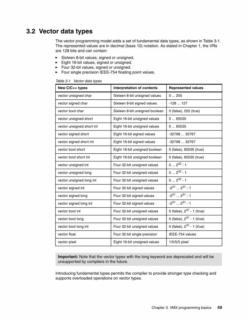
3.2 Vector data typesThe vector programming model adds a set of fundamental data types, as shown in Table 3-1. The represented values are in decimal (base 10) notation. As stated in Chapter 1, the VRs are 128 bits and can contain:

� Sixteen 8-bit values, signed or unsigned.� Eight 16-bit values, signed or unsigned.� Four 32-bit values, signed or unsigned.� Four single precision IEEE-754 floating point values.

Table 3-1 Vector data types

Introducing fundamental types permits the compiler to provide stronger type checking and supports overloaded operations on vector types.

New C/C++ types Interpretation of contents Represented values

vector unsigned char Sixteen 8-bit unsigned values 0 ... 255

vector signed char Sixteen 8-bit signed values -128 ... 127

vector bool char Sixteen 8-bit unsigned boolean 0 (false), 255 (true)

vector unsigned short Eight 16-bit unsigned values 0 ... 65535

vector unsigned short int Eight 16-bit unsigned values 0 ... 65535

vector signed short Eight 16-bit signed values -32768 ... 32767

vector signed short int Eight 16-bit signed values -32768 ... 32767

vector bool short Eight 16-bit unsigned boolean 0 (false), 65535 (true)

vector bool short int Eight 16-bit unsigned boolean 0 (false), 65535 (true)

vector unsigned int Four 32-bit unsigned values 0 ... 232 - 1

vector unsigned long Four 32-bit unsigned values 0 ... 232 - 1

vector unsigned long int Four 32-bit unsigned values 0 ... 232 - 1

vector signed int Four 32-bit signed values -231 ... 231 - 1

vector signed long Four 32-bit signed values -231 ... 231 - 1

vector signed long int Four 32-bit signed values -231 ... 231 - 1

vector bool int Four 32-bit unsigned values 0 (false), 231 - 1 (true)

vector bool long Four 32-bit unsigned values 0 (false), 231 - 1 (true)

vector bool long int Four 32-bit unsigned values 0 (false), 231 - 1 (true)

vector float Four 32-bit single precision IEEE-754 values

vector pixel Eight 16-bit unsigned values 1/5/5/5 pixel

Important: Note that the vector types with the long keyword are deprecated and will be unsupported by compilers in the future.


3.3 Vector keywordsThe programming model introduces new uses for the following five identifiers as simple type specifier keywords:

� vector� __vector� pixel� __pixel� bool

Among the type specifiers used in a declaration, the vector type specifier must occur first. As in C and C++, the remaining type specifiers can be freely intermixed in any order, possibly with other declaration specifiers. The syntax does not allow the use of a typedef name as a type specifier. For example, the following is not allowed:

typedef signed short int16;vector int16 data;

These new uses can conflict with their existing use in C and C++. You can use two methods to deal with this conflict. The vector programming model uses either method. When enabling an application to use vector instructions, we recommend that you avoid using vector in any other context, that is, as a variable name. Inspect the code to see if you need to do a global find and replace before starting to add vector code.

In the programming model, there are two methods for handling these identifiers: the predefine method and the context-sensitive method.

In the predefine method, _vector, _pixel, and bool are added as keywords, while vector and pixel are predefined macros. The identifier bool is already a keyword in C++. To allow its use in C as a keyword, it is treated the same as it is in C++, meaning that the C language is extended to allow bool as a set of type specifiers. Typically, this type maps to unsigned char. To accommodate a conflict with other uses of the identifiers vector and pixel, you can either use #undef or a command line option to remove the predefines. This method is how the GNU C Compiler (gcc) implements these keywords.

In the context-sensitive method, _vector and _pixel are added as keywords without regard to context, while the new uses of vector, pixel, and bool are keywords only in the context of a type. Because vector must be specified before the type, it can be recognized as a type specifier when a type identifier is being scanned. Example 3-4 shows declarations of vector types.

Example 3-4 Specifying vector types

# The vector registers are 128 bits. A vector of unsigned char would allow a single# vector register to contain 16 unsigned chars.vector unsigned char my_val = { 0x00, 0x10, 0x20, 0x30, 0x40, 0x50, 0x60, 0x70,

0x80, 0x90, 0xA0, 0xB0, 0xC0, 0xD0, 0xE0, 0xF0 };

# A vector of unsigned int will allow 4 unsigned ints to occupy one vector register.vector unsigned int my_val2 = { 0x10000000, 0x20000000, 0x30000000, 0x40000000 };

The new uses of pixel and bool occur after vector has been recognized. In all other contexts, vector, pixel, and bool are not reserved, avoiding conflicts such as class vector, typedef int bool and allowing the use of vector, pixel, and bool as identifiers for other uses. This method is how the IBM XLC compiler implements these keywords.


3.4 VMX C extensionsThese extensions readily translate into machine-level instructions as defined by the PowerPC User Instruction Set Architecture (UISA) and Virtual Environment Architecture (VEA). Translation mappings are provided in the detailed descriptions of each function listed in Sections 4.4 and 4.5 of the AltiVec programming manual, PowerPC Microprocessor Family: Programming Environments Manual for 64 and 32-bit Microprocessors. For information about this and other documentation that is available, see “Related publications” on page 119.

3.4.1 Extensions to printf() and scanf()The conversion specifications in control strings for input functions (fscanf, scanf, sscanf) and output functions (fprintf, printf, sprintf, vfprintf, vprintf, vsprintf) are extended to support vector types.

The output conversion specifications have the following general form:

%[<flags>][<width>][<precision>][<size>]<conversion>

where

<flags> ::=<flag-char> | <flags><flag-char><flag-char> ::=<std-flag-char> | <c-sep><std-flag-char> ::= ‘-’ | ‘+’ | ‘0’ | ‘#’ | ‘ ‘<c-sep> ::= ‘,’ | ‘;’ | ‘:’ | ‘_’<width> ::= <decimal-integer> | ‘*’<precision> ::= ‘.’ <width><size> ::= ‘ll’ | ‘L’ | ‘l’ | ‘h’ | <vector-size><vector-size> ::= ‘vl’ | ‘vh’ | ‘lv’ | ‘hv’ | ‘v’<conversion> ::= <char-conv> | <str-conv> | <fp-conv>

|<int-conv> | <misc-conv><char-conv> ::= ‘c’<str-conv> ::= ‘s’ | ‘P’<fp-conv> ::= ‘e’ | ‘E’ | ‘f’ | ‘g’ | ‘G’<int-conv> ::= ‘d’ | ‘i’ | ‘u’ | ‘o’ | ‘p’ | ‘x’ | ‘X’<misc-conv> ::= ‘n’ | ‘%’

The extensions to the output conversion specifications for vector types are shown in bold.

The <vector-size> indicates that a single vector value is to be converted. The vector value is displayed in the following general form:

value1 C value2 C ... C valuen

where C is a separator character defined by <c-sep> and there are 4, 8, or 16 output values depending on the <vector-size> each formatted according to the <conversion>, as follows:

� A <vector-size> of vl or lv consumes one argument and modifies the <int-conv> conversion. It should be of type vector signed int, vector unsigned int, or vector bool int and is treated as a series of four 32-bit components.

� A <vector-size> of vh or hv consumes one argument and modifies the <int-conv> conversion. It should be of type vector signed short, vector unsigned short, vector bool short, or vector pixel and is treated as a series of eight 16-bit components.

� A <vector-size> of v with <int-conv> or <char-conv> consumes one argument. It should be of type vector signed char, vector unsigned char, or vector bool char. It is treated as a series of sixteen 8-bit components.

� A <vector-size> of v with <fp-conv> consumes one argument. It should be of type vector float and is treated as a series of four 32-bit floating-point components.


� All other combinations of <vector-size> and <conversion> are undefined.

The default value for the separator character is a space unless the c conversion is being used. For the c conversion the default separator character is Null (\0). Only one separator character can be specified in <flags>.

Example 3-5 shows some example printf() statements.

Example 3-5 Example printf() statements

vector signed char s8 = vector signed char(‘a’,‘b’,‘c’,‘d’,‘e’,‘f’,‘g’,‘h’,‘i’,‘j’,‘k’,‘l’,‘m’,‘n’,‘o’,‘p’);

vector unsigned short u16 = vector unsigned short(1,2,3,4,5,6,7,8);vector signed int s32 = vector signed int(1, 2, 3, 99);vector float f32 = vector float(1.1, 2.2, 3.3, 4.39501);

printf(“s8 = %vc\n”, s8);printf(“s8 = %,vc\n”, s8);printf(“u16 = %vhu\n”, u16);printf(“s32 = %,2lvd\n”, s32);printf(“f32 = %,5.2vf\n”, f32);

This code produces the following output:s8 = abcdefghijklmnops8 = a,b,c,d,e,f,g,h,i,j,k,l,m,n,o,pu16 = 1 2 3 4 5 6 7 8s32 = 1, 2, 3,99f32 = 1.10 ,2.20 ,3.30 ,4.40

3.4.2 Input conversion specificationsThe input conversion specifications have the following general form:

%[<flags>][<width>][<size>]<conversion>

where

<flags> ::= ‘*’ | <c-sep> [‘*’] | [‘*’] <c-sep><c-sep> ::= ‘,’ | ‘;’ | ‘:’ | ‘_’<width> ::= <decimal-integer><size> ::= ‘ll’ | ‘L’ | ‘l’ | ‘h’ | <vector-size><vector-size> ::= ‘vl’ | ‘vh’ | ‘lv’ | ‘hv’ | ‘v’<conversion> ::= <char-conv> | <str-conv> | <fp-conv> |

<int-conv> | <misc-conv><char-conv> ::= ‘c’<str-conv> ::= ‘s’ | ‘P’<fp-conv> ::= ‘e’ | ‘E’ | ‘f’ | ‘g’ | ‘G’<int-conv> ::= ‘d’ | ‘i’ | ‘u’ | ‘o’ | ‘p’ | ‘x’ | ‘X’<misc-conv> ::= ‘n’ | ‘%’ | ‘[‘

The extensions to the input conversion specification for vector types are shown in bold.


The <vector-size> indicates that a single vector value is to be scanned and converted. The vector value to be scanned is in the following general form:

value1 C value2 C ... C valuen

where C is a separator sequence defined by <c-sep> (the separator character optionally preceded by whitespace characters) and 4, 8, or 16 values are scanned depending on the <vector-size> each value scanned according to the <conversion>, as follows:

� A <vector-size> of vl or lv consumes one argument and modifies the <int-conv> conversion. It should be of type vector signed int * or vector unsigned int * depending on the <int-conv> specification and four 32-bit values are scanned.

� A <vector-size> of vh or hv consumes one argument and modifies the <int-conv> conversion. It should be of type vector signed * or vector unsigned short * depending on the <int-conv> specification and eight 16-bit values are scanned.

� A <vector-size> of v with <int-conv> or <char-conv> consumes one argument. It should be of type vector signed char * or vector unsigned char * depending on the <int-conv> or <char-conv> specification and sixteen 8-bit values are scanned.

� A <vector-size> of v with <fp-conv> consumes one argument. It should be of type vector float * and four 32-bit floating-point values are scanned.

� All other combinations of <vector-size> and <conversion> are undefined.

For the c conversion the default separator character is Null (\0), and the separator sequence does not include whitespace characters preceding the separator character. For anything other than the c conversions, the default separator character is a space, and the separator sequence does include whitespace characters preceding the separator character.

If the input stream reaches end-of-file or there is a conflict between the control string and a character read from the input stream, the input functions return end-of-file and do not assign to their vector argument.

When a conflict occurs, the character causing the conflict remains unread and is processed by the next input operation.

Example 3-6 shows some examples that use the sscanf() routine.

Example 3-6 Example sscanf() statements

sscanf(“ab defghijklm,op”, “%vc”, &s8);sscanf(“a,b, ,d,e,f,g,h,i,j,k,l,m,,,o,p”, “%,vc”, &s8);sscanf(“1 2 3 4 5 6 7 8”, “%vhu”, &u16);sscanf(“1, 2, 3,99”, “%,2lvd”, &s32);sscanf(“1.10 ,2.20 ,3.30 ,4.40” ,“%,5vf” ,&f32);This is equivalent to:vector signed char s8 = vector signed char(‘a’,’b’,’ ’,’d’,’e’,’f’,

‘g’,’h’,’i’,’j’,’k’,’l’,‘m’,’,’,’o’,’p’);

vector unsigned short u16 = vector unsigned short(1,2,3,4,5,6,7,8);vector signed int s32 = vector signed int(1, 2, 3, 99);vector float f32 = vector float(1.1, 2.2, 3.3, 4.4);


3.4.3 Vector functionsThe tables in this section show the C language built-in functions that are available to the application by including <altivec.h> and using the -maltivec and -mabi=altivec options to the GCC compiler.

Table 3-2 provides the list of vector arithmetic functions available to the programmer.

Table 3-2 Vector arithmetic functions

Table 3-3 provides the list of rounding and conversion functions.

Table 3-3 Vector rounding and conversion functions

Function name Usage Valid operands and data types

Vector Absolute Value d = vec_abs(a) any vector signed type

Vector Add d = vec_add(a,b) any vector int or vector float type

Vector Average d = vec_avg(a,b) any vector int type

Vector Multiply Add d = vec_madd(a,b,c) vector float

Vector Maximum d = vec_max(a,b) any vector type

Vector Minimum d = vec_min(a,b) any vector type

Vector Multiply Sum d = vec_msum(a,b,c) vector charvector short

Vector Multiply Even d = vec_mule(a,b) vector charvector short

Vector Negative Multiply Subtract d = vec_nmsub(a,b,c) vector float

Vector Subtract d = vec_sub(a,b) any vector type

Vector Sum Saturated d = vec_sums(a,b) vector signed int

Function name Usage Valid operands and data types

Vector Ceiling d = vec_ceil(a) vector float

Vector Convert from Fixed-Point Word

d = vec_ctf(a,b) vector int

Vector Floor d = vec_floor(a) vector float

Vector Round d = vec_round(a) vector float

Vector Truncate d = vec_trunc(a) vector float


Table 3-4 provides the list of floating-point estimate functions.

Table 3-4 Vector floating-point estimate functions

Table 3-5 provides the list of vector compare functions.

Table 3-5 Vector compare instructions

Function name Usage Valid data types

Vector Is 2 Raised to the Exponent Estimate Floating-Point

d = vec_expte(a) vector float

Vector Log2 Estimate Floating-Point

d = vec_loge(a) vector float

Vector Reciprocal Estimate d = vec_re(a) vector float

Vector Reciprocal Square Root Estimate

d = vec_rsqrte(a) vector float


Vector Compare Bounds Floating-Point

d = vec_cmpb(a,b) d vector bool inta,b vector float

Vector Compare Equal d = vec_cmpeq(a,b) d vector bool inta,b any vector int or vector float type

Vector Compare Greater Than or Equal

d = vec_cmpge(a,b) d vector bool inta,b vector float

Vector Compare Greater Than d = vec_cmpgt(a,b) d vector bool inta,b any vector int or vector float type

Vector Compare Less Than or Equal

d = vec_cmple(a,b) d vector bool inta,b vector float

Vector Compare Less Than d = vec_cmplt(a,b) d vector bool inta,b any vector int or vector float type

All Elements Equal d = vec_all_eq(a,b) d inta,b any vector type

All Elements Greater Than or Equal d = vec_all_ge(a,b) d inta,b any vector type

All Elements Greater Than d = vec_all_gt(a,b) d inta,b any vector type

All Elements Less Than or Equal d = vec_all_le(a,b) d inta,b any vector type

All Elements Less Than d = vec_all_lt(a,b) d inta,b any vector type

All Elements Not a Number d = vec_all_nan(a) d inta vector float

All Elements Not Equal d = vec_all_ne(a,b) d inta,b any vector type


All Elements Not Greater Than or Equal

d = vec_all_nge(a,b) d inta,b vector float

All Elements Not Greater Than d = vec_all_ngt(a,b) d inta,b vector float

All Elements Not Less Than or Equal

d = vec_all_nle(a,b) d inta,b vector float

All Elements Not Less Than d = vec_all_nlt(a,b) d inta,b vector float

All Elements Numeric d = vec_all_numeric(a) d inta vector float

Any Element Equal d = vec_any_eq(a,b) d inta,b any vector type

Any Element Greater Than or Equal d = vec_any_ge(a,b) d inta,b any vector type

Any Element Greater Than d = vec_any_gt(a,b) d inta,b any vector type

Any Element Less Than or Equal d = vec_any_le(a,b) d inta,b any vector type

Any Element Less Than d = vec_any_lt(a,b) d inta,b any vector type

Any Element Not a Number d = vec_any_nan(a) d inta vector float

All Elements Not Equal d = vec_any_ne(a,b) d inta,b any vector type

Any Element Not Greater Than or Equal

d = vec_any_nge(a,b) d inta,b vector float

Any Element Not Greater Than d = vec_any_ngt(a,b) d inta,b vector float

Any Element Not Less Than or Equal

d = vec_any_nle(a,b) d inta,b vector float

Any Element Not Less Than d = vec_any_nlt(a,b) d inta,b vector float

Any Element Out of Bounds d = vec_any_out(a,b) d inta,b float



Table 3-6 provides the list of vector logical functions.

Table 3-6 Vector logical functions

Table 3-7 provides the list of vector rotate and shift functions.

Table 3-7 Vector rotate and shift functions

Table 3-8 provides the list of vector load and store functions.

Table 3-8 Vector load and store functions


Vector Logical AND d = vec_and(a,b) any vector type

Vector Logical NOR d = vec_nor(a,b) any vector type

Vector Logical OR d = vec_or(a,b) any vector type

Vector Logical XOR d = vec_xor(a,b) any vector type


Vector Rotate Left d = vec_rl(a,b) any vector int type

Vector Shift Left d = vec_sl(a,b) any vector int type

Vector Shift Right d = vec_sr(a,b) any vector int type


Vector Load Indexed d = vec_ld(a,b) a any int typeb any pointer or vector pointerd corresponding vector type of b

Vector Load Element Indexed d = vec_lde(a,b) a any int typeb any pointer typed corresponding vector type of b

Vector Load for Shift Left (for misaligned data)

d = vec_lvsl(a,b) a any int typeb pointer to any typed vector unsigned char

Vector Load Shift Right d = vec_lvsr(a,b) a any int typeb pointer to any typed vector unsigned char

Vector Store Indexed vec_st(a,b,c) b any int typec any pointer or vector pointera corresponding vector type of c

Vector Store Element Indexed vec_ste(a,b,c) b any int typec any pointera corresponding vector type of c


Table 3-9, Table 3-10, and Table 3-11 provide the list of data manipulation and formatting functions.

Table 3-9 Vector pack and unpack functions

Table 3-10 Vector merge functions

Table 3-11 Vector permute and select functions

3.4.4 Summary of VMX C extensionsBefore proceeding with vector enablement, check if any vector keywords (especially vector or pixel) are used as variable names in program code. It is easiest to do a global find and replace to remove keywords before you add vector data types and functions.

There is no add or multiply operations available for 64-bit floating-point (type double) or 64-bit integer (type long long) operands.

There is no multiply operation available for 32-bit integer (types int or long int) operands. However, 32-bit integer addition is supported.

There is a wide range of functions available to hand-optimize code, but most are best left for preprocessing and compiler tools. The most useful tools for hand coding are the arithmetic functions; load, store, and splat (broadcast) functions to initialize vectors; and functions that support branching (compare, select, and permute).


Vector Pack d = vec_pack(a,b) a,b vector short or intd vector char or short

Vector Pack Pixel d = vec_packpx(a,b) a,b vector unsigned intd vector pixel

Vector Unpack High Element d = vec_unpackh(a) a vector chard vector short


Vector Merge High d = vec_mergeh(a,b) any vector type

Vector Merge Low d = vec_mergel(a,b) any vector type


Vector Permute d = vec_perm(a,b,c) a,b,d any vector typec vector unsigned char

Vector Conditional Select d = vec_sel(a,b,c) a,b,d any vector typec bool, char, short or int


Chapter 4. Application development tools

This chapter describes applications development tools available for programming the PowerPC 970 microprocessor. It includes options that are available with the GNU compiler collection and provides details on the support provided by XLC/C++ Enterprise Edition for Linux.

4


4.1 GNU compiler collectionThe GNU Compiler Collection (gcc) is the de facto standard compiler set for Linux. All Linux distributions provide some version of gcc. Some of the Linux distributions, provide gcc compilers with direct support for the PowerPC 970 through processor-specific compiler options. The gcc compiler includes vector exploitation through the C language extensions as described in 3.4.3, “Vector functions” on page 64, often referred to as built-in functions. At this time gcc does not offer any automatic vectorization capabilities.

This paper does not provide comprehensive documentation for the gcc compiler. However, it does address features directly related to the PowerPC 970 microprocessor found in the IBM Eserver BladeCenter JS20. For complete gcc compiler documentation, see the many online resources available at:

http://gcc.gnu.org/onlinedocs/

4.1.1 Processor-specific compiler optionsThe following options to the gcc compiler are necessary to support the PowerPC 970 microprocessor:

� -mcpu=cputype

Enables compiler support for architecture type, register usage, choice of mnemonics, and instruction scheduling parameters for machine cputype. While many options exist for cputype, the follow are values are pertinent for this discussion: 970, G5, power4, power5 and common. The 970 keyword specifies the IBM PowerPC 970 microprocessor, which is used in the IBM Eserver BladeCenter JS20 and, in general, would be the preferred option. G5 can also be used because the Apple Power MAC G5 uses the IBM PowerPC 970 and as such both are interchangeable. The power4 and power5 keyword refer to the POWER4 and POWER5™ processor architectures respectively. The IBM PowerPC 970 microprocessor processor derives from POWER4 and, in some cases, power4 can produce better performance on the IBM PowerPC 970 microprocessor. However, this in general would be the exception and not the rule. The option common is used to suppress the generation of any processor unique instructions by restricting the instructions to the subset of instructions common to both the POWER and PowerPC architectures.

� -mtune=cputype

Sets the instruction scheduling parameters for machine type cputype, but does not set the architecture type, register usage, or choice of mnemonics, as -mcpu=cputype would. The same values for cputype are used for -mtune as for -mcpu. If both are specified, the code generated uses the architecture, registers, and mnemonics set by -mcpu but the scheduling parameters set by -mtune.

4.1.2 Compiler options for VMXThe following options to the gcc compiler are necessary to take advantage of the vectorization capability of the PowerPC 970.

� -maltivec | -mno-altivec

Enables or disables the use of the vector built-in functions. The use of -maltivec is mandatory for vector applications. Default is -mno-altivec.

� -mabi=altivec

Extends the current ABI to include AltiVec ABI extensions. This does not change the default ABI. Instead it adds the AltiVec ABI extensions to the current ABI. In general this is not needed for the VMX applications on the IBM Eserver BladeCenter JS20.


http://gcc.gnu.org/onlinedocs/

4.1.3 Suggested compiler optionsThe following tuning options are suggested options to support vectorization on the PowerPC 970 microprocessor.

JS20 specific tuningFor processor-specific tuning the follow set of compilers switches are suggested:

gcc -mcpu=970 -m32|-m64 -O2|-O3 OtherFlags a.c ...

In this set of compilers, -m32 or -m64 is used to specify 32- or 64-bit application binaries, -O2 or -O3 is used to suggest the use of either optimization levels 2 or 3, and OtherFlags could be any other gcc compiler option(s). The -mcpu=970 instructs the compiler to generate PowerPC 970 specific instructions so the binaries generated are not guaranteed to be compatible with other processors in the POWER/PowerPC family.

To produce binaries that are compatible with all POWER/PowerPC based processors, yet biased for the PowerPC 970 processor, the following is suggested:

gcc -mcpu=common -mtune=970 -m32|-m64 -O2|-O3 OtherFlags a.c ...

In this example, -mtune=970 instructs the compiler to optimize the code for PowerPC 970 specific instruction scheduling. This is important because not all PowerPC implementations are the same when it comes to the degree of superscalar implementation (number of instruction pipelines). The goal is to produce an object binary that arranges the independent and dependent instructions in a way as to not cause a bottleneck, yet still reach a high degree of parallel instruction execution. The code in Example 2-3 on page 45 is an example of how we do not want the code to be generated. We would not want these three instructions back-to-back because of dependency. With the tune option, we are asking the compiler to put as much distance (independent instructions) between each one. By doing this the cmpwi instruction would not have to wait for the load to finish before getting a chance to compare it to zero. As stated in Chapter 1, there is a two cycle load-to-use penalty and that is assuming a cache hit. If the compiler can move the lwz instruction up sooner in the binary, the cmpwi instruction does not have to wait. The same is true for the beq instruction. It would not be speculative execution if the result of the cmpwi is know at the time the beq is executed.

Compiling for VMX exploitationCurrently the PowerPC 970 processor is the only POWER based processor which supports VMX. As such vectorized binaries are only compatible with the PowerPC 970 processor. The following compiler switches are suggested for VMX applications:

gcc -mcpu=970 -maltivec -m32|-m64 -O2|-O3 OtherFlags a.c ...

The -maltivec is necessary to use the built in functions and to produce the vector instructions. OtherFlags could be any other gcc compiler option.

4.2 XL C/C++ and XL FORTRAN compiler collectionsThe XL FORTRAN Enterprise Edition V9.1 for Linux and XL C/C++ Enterprise Edition V 7.0 for Linux compilers include support for code optimizations designed to take full advantage of the VMX instruction set included as part of the PowerPC 970 microprocessor. Both the C/C++ and FORTRAN compilers support the automatic parallelization of loop and non-loop language constructs using the vector instruction set. This is known as automatic short-vectorization or automatic SIMD vectorization. Additionally, The C/C++ compiler supports the vector builtin functions as defined by the Motorola C/C++ AltiVec extensions.

Chapter 4. Application development tools 71

Short versus long vectorizationIn this paper, the term vectorization refers specifically to short vectorization. The XL C/C++ and XL FORTRAN compilers also support automatic generation of long vectorization. This refers to parallel computation carried out on an arbitrarily long array of data. Support for long vectorization is provided via the -qhot=vector option. For more information about short versus long vectorization, see the XL FORTRAN Users Guide.

VMX support on the SuSE and RedHat Linux Operating SystemsThe XL FORTRAN Enterprise Edition V9.1 and XL C/C++ Enterprise Edition V7.0 support SuSE Linux Enterprise Server 9 and RedHat Linux 4, running on the IBM Eserver BladeCenter JS20. If you are running RedHat Linux 3, the compiler defaults to not generate any vector code. The compiler implicitly adds the -qnoenablevmx option. For the RedHat Linux 3 system, you have to specify both -qhot=ppc970 and -qenablevmx.

VMX support on the AIX Operating SystemThe XL FORTRAN Enterprise Edition V9.1 and XL C/C++ Enterprise Edition V7.0 support the AIX operating system running on the IBM Eserver BladeCenter JS20. To provide optimization for the vectorization and tuning of the PowerPC 970 microprocessor use the -qarch=ppc64grsq option, which generates correct code for all processors in the ppc64grsq group of processors: RS64 II, RS64 III, POWER3™, POWER4, POWER5, and PowerPC970. Use the option -qhot=vector to generate vector instructions.

Compiling C/C++ code with VMX builtinsSource code that contains vector data types and builtin functions requires that you specify the -qaltivec compiler option. Additionally, you must specify -qarch=ppc970 at optimization levels -O0 to -O3.

For example, if you are using SuSE Linux Enterprise Server 9 on a IBM Eserver BladeCenter JS20 blade, the following are both valid compilation commands:

xlc -qaltivec -O3 -qarch=ppc970 a.c

or

xlc -qaltivec -O4 a.c

Compiling for automatic vectorizationThe XL C/C++ and FORTRAN compilers can automatically transform loops and some non-loop programming constructs into parallel code using vector instructions. These code transformations are part of the High Order Transformation phase of the optimization process. Specifying -qhot=simd enables automatic vectorization. The -qhot=simd suboption is implied when you specify -qhot=ppc970 option on SuSE Linux Enterprise Server 9 and RedHat Linux 4. For example, the following performs automatic vectorization:

xlc -qhot=ppc970 a.c

On RedHat Enterprise 3 system use:

xlc -qhot=ppc970 -qenablevmx a.c

If there are vectorizable statements in program.f, either of the following results in automatic short vectorization:

xlf -O2 -qarch=ppc970 -qhot program.f

or

xlf -O4 a.f


4.2.1 Options controlling vector code generationThe following are some of the options available for optimizing code for vectorization.

� -qaltivec

This option enables compiler support for the vector data types and builtin functions. This option requires that you specify both -qarch=ppc970 and -qenablevmx. This option has no effect on automatic vectorization.

� -qarch=[ppc970|auto]

Specifies the PowerPC 970 as the target architecture for VMX code generation . You must specify -qarch=ppc970 or -qarch=auto for the -qaltivec or -qhot=simd compiler options to be effective. Optimization levels -O4 and -O5 automatically specify -qarch=auto enabling VMX code transformations.

� -qenablevmx/-qnoenablevmx

Controls the generation of vector instructions, applying to both builtin functions and automatic vectorization. On SuSE Linux 9 and RedHat Enterprise Linux 4 the default option is -qenablevmx, while on RedHat Enterprise Linux 3 the default is -qnoenablevmx. Can also be used to turn off all vector code generation by the compiler. Allows you to prevent the compiler from generating vector instructions in a PowerPC 970 environment that does not fully support VMX.

� -qhot=[simd|nosimd]

Instructs the compiler to perform high order loop analysis and transformations. The simd suboption further instructs the compiler to perform automatic vectorization of loops. The -qhot=simd suboption is implied when you specify -qhot. Optimization levels -O4 and -O5 automatically specify -qarch=simd. You can use the -qhot=nosimd to prevent automatic vectorization of loops, while not preventing other loop transformations.

4.2.2 Alignment-related attributes and builtinsThe XL compiler family can perform interprocedural alignment analysis as part of link phase optimization. Interprocedural alignment analysis can calculate and propagate alignment information in order to minimize the code required to handle misaligned data.

The alignx builtinThe syntax of alignx is:

C/C++: __alignx(<alignment>, <address expression>)FORTRAN: call alignx(<alignment>, <address expression>)

The alignx builtin function is available both in FORTRAN and C/C++. By inserting an alignx builtin at a specific place in the source code, you guarantee that the address expression at the particular execution point is aligned on an <alignment> boundary. Specifically, at the call point to alignx, the user asserts that the second argument to alignx modulo the first argument is zero.

Use the alignx directive to assist the compiler in generating better code in misaligned cases. However, wrong alignx information can lead to incorrect results.


Example 4-1 provides examples of how to use the alignx call.

Example 4-1 Use of the alignx call

FORTRAN:subroutine vec(a, b, c) integer a(200), b(200), c(200) call alignx(16, a(1)) call alignx(16, b(1)) call alignx(16, c(1)) do n = 1, 200 c(n) = a(n) + b(n) enddoend subroutine

C/C++:void vec(int a[200], b[200], c[200]){

int n;__alignx(16, a);__alignx(16, b);__alignx(16, c);for (n=0; n<00; n++)

c[n] = a[n] + b[n];}

The aligned attributeThe syntax of aligned is:

C/C++: <type> <variable> __attribute__ ((aligned(<alignmnent>))) ;

The aligned attribute is a GNU language extension. It instructs the compiler to place the variable at a memory location that is aligned on <alignment> bytes. The XL C/C++ compiler is able to align all file scope and function scope variables on the 16-byte boundary. For externally declared variables, the XL compiler can only assume natural alignments when whole program analysis is enabled, such as at optimization levels -O4 or -O5.

int array[256] __attribute__((aligned(16)));

Example 4-2 illustrates the use of the alignx directives and the data dependency assertion flags discussed previously. This program consists of three routines in two C files, test.c shown in Example 4-2 and main.c shown in Example 4-3 on page 75.

Example 4-2 test.c program

int test(int *pb, int *pc){

int i;int sum = 0;__alignx(16, pb);__alignx(16, pc-2);for (i = 0; i < 252; i++)

sum += pb[i] + pc[i];return sum;

}


Example 4-3 main.c program

int b[128] __attribute__ ((aligned(16)));int c[128] __attribute__ ((aligned(16)));

void initialize(){

int i;for (i = 0; i < 256; i++){

b[i] = i;c[i] = i*i;

}}int main(){

int i, sum;initialize();sum = test(b, c+2);printf("sum = %d\n", sum);

}

Example 4-4 compiles the two files at -O3, which does not do any whole program analysis.

Example 4-4 Compilation example

xlc -qarch=ppc970 -qtune=ppc970 test.c -O3 -qhot -qreport -c xlc -qarch=ppc970 -qtune=ppc970 main.c -O3 -qhot -qreport -cxlc main.o test.o -o example

Without whole-program analysis (or inter-procedural analysis), the two __alignx directives in test() are essential for conveying the alignment information of pb and pc to the compiler.

The first alignx directive asserts that pb is aligned on a 16-byte boundary. The second alignx directive asserts that (pc - 2) is aligned on a 16-byte boundary. According to the definition of alignx, the second alignx means:

(pc-2) mod 16 == 0

Because pc is an integer pointer, this means the address pc is always at the 8th byte within a 16-byte boundary.


Using the -qreport option, the compiler generates output to the screen about the vectorized loop in test() as shown in Example 4-5.

Example 4-5 Output from the -qreport option

1586-542 (I) <SIMD info> SIMDIZABLE (Loop index 1 on line 6 with nest-level 0 and iteration count 252.)1586-543 (I) <SIMD info> Total number of loops considered <"1">. Total number of loops simdized <"1">. 1 | long test ( struct $ * pb, struct $ * pc ) { 3 | sum = 0; 6 | if (!1) goto lab_4; __alignx(16,((char *)pb + (4)*(0))) 4 | __alignx(16,pb) 5 | __alignx(16,((char *)pc - 8)) $.VTEMP0 = splice((vector long <4>)(0),(vector long <4>)(0) + (align(*(pb + -2 * 4 / 196612),*(pb + 2 * 4 / 196612),8) + *(pc + 0 * 4 / 196612)),8); $.oldSPCopy0 = *(pb + 2 * 4 / 196612); $.CIV1 = (long) 0; 6 | do { /* id=1 guarded */ /* ~3 */ /* bump-normalized */ /* independent */ 7 | $.VTEMP0 = $.VTEMP0 + (align($.oldSPCopy0,*(pb + $.CIV1 * 4 + 6 * 4 / 196612),8) + *(pc + $.CIV1 * 4 + 4 * 4 / 196612)); 6 | $.oldSPCopy0 = *(pb + $.CIV1 * 4 + 6 * 4 / 196612); $.CIV1 = $.CIV1 + 1; } while ((unsigned) $.CIV1 < 62u); /* ~3 */ $.VTEMP0 = splice($.VTEMP0 + (align(*(pb + 250 * 4 / 196612),*(pb + 254 * 4 / 196612),8) + *(pc + 252 * 4 / 196612)),$.VTEMP0,8); sum = reduct($.VTEMP0); lab_4: 8 | rstr = sum; return rstr; 9 | } /* function */

Knowing the alignment of a pointer reference is crucial. If the two alignx directives are removed from the routine test(), sub-optimal code is generated because the compiler must assume the worst scenario (that the pointers can only be at 1 byte alignment). In the absence of the alignx directives, the compiler creates two version of the loop, a vectorized version and a scalar version. A run time check for the alignment of pb and pc are inserted into the code, and the vectorized version is chosen only if pb and pc are aligned on a 16-byte boundary. Because arrays b and c as declared in main.c are aligned on a 16-byte boundary via the aligned attributes, it is not possible for pc to be aligned on a 16-byte boundary.

Compiling the code in Example 4-5 at optimization level -O5, where the compiler is capable of propagating inter-procedural alignment analysis, the __alignx directives would not be needed to produce vectorized code.

4.2.3 Data dependency analysisData dependency analysis is essential when the user code is dominated by pointer accesses. The interprocedural analysis in the XL compiler disambiguates all pointer references and calls. Thus, you should compile at the highest optimization level to receive the benefits of such analysis. However, in the case when compile time is a concern, you might wish to compile at a lower optimization.


The following might be useful to provide data dependency assertion to the compiler.

-qalias=<option>

The <option> specifies the aliasing assertion to be applied to your compilation unit. The available options are specific to the language:

� For the C/C++ compiler:

addrtaken | noaddrtaken Variables are disjoint from pointers unless their address is taken.

allptrs | noallptrs If noallptrs is specified, pointers are never aliased. Therefore no two pointers point to the same address.

ansi | noansi If ansi is specified, pointers can only point to an object of the same type. ansi is the default for the C/C++ compilers. This option has no effect unless you also specify the -O option.

typeptr | notypeptr If notypeptr is specified, pointers to different types are never aliased.

� For the FORTRAN compiler:

aryovrlp | noaryovrlp Indicates whether the compilation unit contains any array assignments between storage-associated arrays.

intptr | nointptr Indicates whether the compilation unit contains any INTEGER pointer statements

pteovrlp | nopteovrlp Indicates whether two pointer variables can be used to refer to any data objects that are not pointer variables, or whether two pointer variables can be used to refer to the same storage location.

std | nostd Indicates whether the compilation unit contains any nonstandard aliasing

Example 4-6 on page 78 illustrates the need for the data dependency assertion flag, -qalias=allptrs.


Example 4-6 Use of -qalias=allptrs

#include <stdlib.h>#include <stdio.h>

int main(){

int i;float sum = 0.0;const int ITER = 1024*256;const int VDIM = 1024;

float *ra, *rb, *rc, *rd, *re;

ra = (float *) malloc(sizeof(float)*VDIM);rb = (float *) malloc(sizeof(float)*VDIM);rc = (float *) malloc(sizeof(float)*VDIM);rd = (float *) malloc(sizeof(float)*VDIM);re = (float *) malloc(sizeof(float)*VDIM);

// first for loop for (i=0; i< VDIM; i++)

{ ra[i] = i/2.3 + 2; rb[i] = 1.716*i; rc[i] = 3.141*i+5; } printf(">>> below Loop SIMDizes with -qalias=allptrs <<< \n"); // second for loop for (i=0; i< VDIM; i++) { re[i] = ra[i]*rb[i] + rc[i]*rd[i]; rd[i] = ra[i] + rb[i]; } // third for loop for (i=0; i < VDIM; i++) sum += re[i] + rd[i];

printf("sum = %f\n", sum);}

The command to compile this file, assuming that it is called program.c, is as follows:

xlc -qarch=ppc970 -qtune=ppc970 program.c -O3 -qhot -qalias=noallptrs -qreport -c xlc main.o -o example2

The -qalias=noallptrs flag indicates to the compiler that none of the pointers are aliased with each other. There are three for loops in the main() routine. The second and third for loops are fused into one loop and the resulting loop is vectorized. Because all the pointers are disjoint as guaranteed by the -qalias=noallptrs flag, the vectorized loop is as shown in Example 4-7 on page 79.


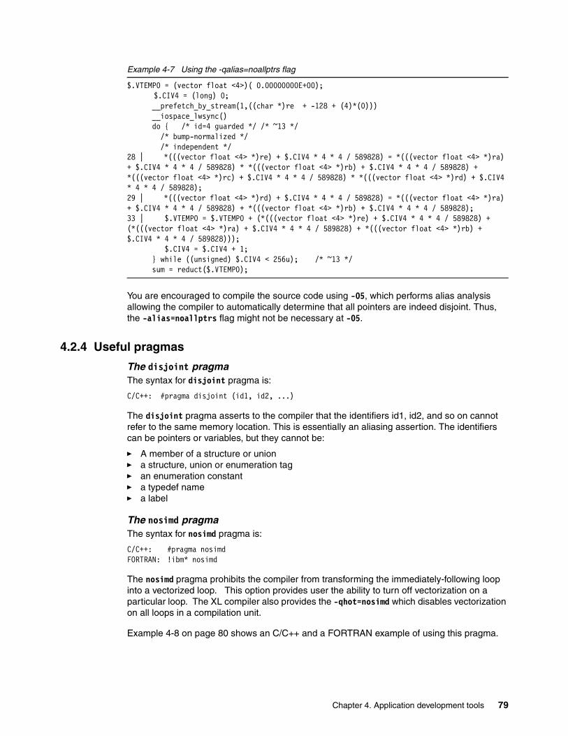
Example 4-7 Using the -qalias=noallptrs flag

$.VTEMP0 = (vector float <4>)( 0.00000000E+00);$.CIV4 = (long) 0;

__prefetch_by_stream(1,((char *)re + -128 + (4)*(0))) __iospace_lwsync() do { /* id=4 guarded */ /* ~13 */ /* bump-normalized */ /* independent */28 | *(((vector float <4> *)re) + $.CIV4 * 4 * 4 / 589828) = *(((vector float <4> *)ra) + $.CIV4 * 4 * 4 / 589828) * *(((vector float <4> *)rb) + $.CIV4 * 4 * 4 / 589828) + *(((vector float <4> *)rc) + $.CIV4 * 4 * 4 / 589828) * *(((vector float <4> *)rd) + $.CIV4 * 4 * 4 / 589828);29 | *(((vector float <4> *)rd) + $.CIV4 * 4 * 4 / 589828) = *(((vector float <4> *)ra) + $.CIV4 * 4 * 4 / 589828) + *(((vector float <4> *)rb) + $.CIV4 * 4 * 4 / 589828);33 | $.VTEMP0 = $.VTEMP0 + (*(((vector float <4> *)re) + $.CIV4 * 4 * 4 / 589828) + (*(((vector float <4> *)ra) + $.CIV4 * 4 * 4 / 589828) + *(((vector float <4> *)rb) + $.CIV4 * 4 * 4 / 589828))); $.CIV4 = $.CIV4 + 1; } while ((unsigned) $.CIV4 < 256u); /* ~13 */ sum = reduct($.VTEMP0);

You are encouraged to compile the source code using -O5, which performs alias analysis allowing the compiler to automatically determine that all pointers are indeed disjoint. Thus, the -alias=noallptrs flag might not be necessary at -O5.

4.2.4 Useful pragmas

The disjoint pragma The syntax for disjoint pragma is:

C/C++: #pragma disjoint (id1, id2, ...)

The disjoint pragma asserts to the compiler that the identifiers id1, id2, and so on cannot refer to the same memory location. This is essentially an aliasing assertion. The identifiers can be pointers or variables, but they cannot be:

� A member of a structure or union� a structure, union or enumeration tag� an enumeration constant� a typedef name� a label

The nosimd pragmaThe syntax for nosimd pragma is:

C/C++: #pragma nosimdFORTRAN: !ibm* nosimd

The nosimd pragma prohibits the compiler from transforming the immediately-following loop into a vectorized loop. This option provides user the ability to turn off vectorization on a particular loop. The XL compiler also provides the -qhot=nosimd which disables vectorization on all loops in a compilation unit.

Example 4-8 on page 80 shows an C/C++ and a FORTRAN example of using this pragma.


Example 4-8 The nosimd pragma

FORTRAN:subroutine vec(a, b) real*4 a(200), b(200) !ibm* nosimd forall (n=1:200) b(n) = b(n) * a(n)end subroutine

C/C++:void vec(float a[200], float b[200]) { int n; #pragma nosimd for (n=0; n<00; n++) b[n] = b[n] * a[n];}

4.2.5 Generating vectorization reportsThe compiler provides listing and report flags that can be used to examine the results of compilation, using -qreport and -qlist. Both compiler options send their output to a file with the .lst extension. The name of the output file depends on the optimization level. When whole program analysis is disabled, such as when compiling the code at -O0 to -O3, the output file is <sourcefile>.lst. At -O4 and -O5, the two files a.lst and <sourcefile>.lst are produced. However, only a.lst contains the final results of the compilation. Note that <sourcefile.lst> contains the intermediate code, before whole program analysis was performed.

-qlist Produces a pseudo assembly listing of the result of the compilation, also known as the object listing

-qreport Produces transformation reports on the high level loop optimizations performed by the -qhot and -qsmp options. This produces a summary of the loops considered for automatic vectorization, a list of loops vectorized and not vectorized and reasons for them.

Example 4-8 illustrates these two flags.

Example 4-9 Vectorization reports, code example

int a[256], b[256],c[256];void test(){

int i;for (i = 0; i < 256; i++)

a[i] = b[i] + c[i];}int main(){

int i;test();for (i = 0; i < 256; i++)printf("a = %d", a[i]);

}

We used the following command to compile our program, called test.c.

xlc -O5 -qreport -qlist test.c


The output was written to the file a.lst and is shown in Example 4-10.

Example 4-10 Vectorization reports, a.lst file

1586-541 (I) <SIMD info> NON-SIMDIZABLE: other misc reasons. (Loop index 1 on line 10 with nest-level 0 and iteration count 256.)1586-542 (I) <SIMD info> SIMDIZABLE (Loop index 2 on line 4 with nest-level 0 and iteration count 256.)1586-543 (I) <SIMD info> Total number of loops considered <"2">. Total number of loops simdized <"1">.

7 | long main ( ) {4 | if (!1) goto lab_6;

__alignx(16,((char *)&a + (4)*(0))) __alignx(16,((char *)&b + (4)*(0))) __alignx(16,((char *)&c + (4)*(0))) $.2CIV0 = (long) 0; do { /* id=2 guarded */ /* ~7 */ /* bump-normalized */ /* independent */

5 | __dcbt(((char *)&a + (0 + 256) + (4)*($.2CIV0 * 4))) a[$.2CIV0 * 4] = b[$.2CIV0 * 4] + c[$.2CIV0 * 4];

4 | $.2CIV0 = $.2CIV0 + 1; } while ((unsigned) $.2CIV0 < 64u); /* ~7 */ lab_6:

10 | if (!1) goto lab_4; $.CIV1 = 0; __alignx(16,((char *)&a + (4)*(0))) do { /* id=1 guarded */ /* ~3 */ /* bump-normalized */

11 | printf("a = %d",a[$.CIV1]);10 | $.CIV1 = $.CIV1 + 1;

} while ((unsigned) $.CIV1 < 256u); /* ~3 */ lab_4: rstr = 0;

12 | return rstr; } /* function

In Example 4-10, the compiler has inlined test() into main() and has vectorized the loop in test(). Loops are identified by their loop id and the line number in which they occur. The line numbers are listed on the left side, and are followed by a “|.” Loop IDs can be found by looking for id=<number> in the C pseudo-code. To see the vector intrinsics that were generated for this code, we would have to look in the file, test.lst.


Chapter 5. Vectorization examples

What does it take to write VMX-enabled code? This chapter discusses the tools that you can use to understand vector functions and to convert scalar code into vectorized code.

5


5.1 Explanation of the examplesThe examples presented here are written in C because C is the language used to access the vector function extensions. Similar tools are also available to work with FORTRAN programs.

As discussed earlier in previous chapters, you have to collect profiling information for an application and an associated set of problems. Then, you can focus on the time-consuming loops that can best exploit vector instructions. At that point, you can use the information in this chapter to help with vectorizing these code hot spots.

This chapter first discusses some common loop fragments that present opportunities for vectorization (especially, the automatic, compiler-driven form of vectorization specific to short vectors). It also reports speedups from automatic and hand-coded vectorization of those loops, compared to the corresponding scalar loop performance. Later sections present some of the conditions that prevent loop vectorization, along with suggested remedies to allow vectorization when possible.

Scalar performance for the PowerPC 970 processor is discussed in the IBM Redbook, The POWER4 Processor: Introduction and Tuning Guide, SG247041. A reasonable goal for scalar code is to reach half of peak performance. Understanding scalar performance of the processor is helpful in understanding what reasonable performance improvement and effort to expect from vector optimizations. Also, simple use of Amdahl’s Law with the results from execution profiling can also help quantify the expected performance improvement. If an evaluation finds that a candidate loop is really performing at substantially less than peak, it might be worth trying scalar optimization first.

Based on the hardware specifications for a PowerPC 970 processor, you might expect a peak speedup of two times from scalar to vector operations for 32-bit operands, four times for 16-bit integer operands, and for eight times for 8-bit (including character) integer operands. On the one hand, because of limitations in scheduling scalar instructions and memory bottlenecks, vector-optimized programs can exceed these performance expectations. On the other hand, because of the overhead associated with real-world programming (not every line of code in a program is part of a loop), vector-optimized programs can also fall short of expectations. Optimizing the scalar performance of a loop needs to be considered as an alternative to vector enablement, but it is up to the judgement of the programmer to balance the effort needed to the performance improvement expected.

These examples are loops that can be automatically vectorized through the use of the VAST optimizer, vcc. This optimizer depends on C compilers that recognize VMX extensions (gcc version 3.3, with patches, or later is used by vcc and XLC/C++ Compiler version 7.0 or later is used by vlc) or directly through the XLC/C++ Compiler compiler, xlc version 7.0 or later. These examples are intended to help both in identifying candidate loops in hot spots within a program and in estimating the speedups that could be expected by VMX optimization.Later examples show loops that will not vectorize and suggests remedies (relatively minor code changes or compiler directives or command line options).

We tested loops with the VAST C optimizer (vcc or vlc) and an XLC/C++ Compiler (version 7.0). Timings were done on a IBM Eserver BladeCenter JS20 running the Linux kernel 2.6.5-7.51-pseries64. Raw timing data is provided as part of the tarball included with this paper.


5.1.1 Command-line optionsThe examples in this chapter use the following command-line options:

� Options to compile the examples with gcc in scalar mode:

gcc -O3 -mcpu=970 -mtune=970 <filenm>

� Options to compile the examples with xlc in scalar mode:

xlc -O3 -qarch=ppc970 -qtune=ppc970 <filenm>

� Options to compile the examples with vcc:

vcc -O3 -Wv,”-L3,-g3,-Vmessages,-lvast.lst” -maltivec -mcpu=970 -mtune=970 <filenm>

� Options using vlc:

vlc -O5 -Wv,”-L3,-g3,-Vmessages,-lvast.lst” -qarch=ppc970 -qtune=ppc970 -qreport <filenm>

� Options to run through the vectorization stage of the VMX-enabled XLC/C++ Compiler compiler, xlc:

xlc -O5 -qarch=ppc970 -qtune=ppc970 -qreport <filenm>

In all cases, this option enables the compiler and optimizer to try vectorization on all loops of the supplied code.

� Options to compile hand-modified, VMX-enabled code through xlc:

xlc -O3 -qarch=ppc970 -qtune=ppc970 -qaltivec <filenm>

� Options to compile hand-modified, VMX-enabled code through gcc:

gcc -O3 -mcpu=970 -mtune=970 -maltivec -mabi=altivec <filenm>

5.2 Vectorized loopsBoth the VAST optimizer, vastcav, and the XLC/C++ Compiler compiler for VMX, xlc, were able to vectorize all loop examples presented, though some typical C coding syntax had to be avoided in order to ensure vectorization. For the complete listing of the code involved, including variable declarations and context, see files Ex1.c, Ex2.c, VEx1.c, VEx2.c, HVEx1.c, HVEx2.c, VACEx1.lst and VACEx2.lst in the tarball that comes with this paper.

Note that using vcc or vlc to compile produces equivalent performance. Compiling examples hand-coded for VMX optimization with gcc or xlc also had similar performance (with the edge going to xlc). Speedups from all five combinations: vcc driver, vlc driver, hand coded using gcc, hand coded using xlc and xlc with automatic vectorization are reported. For any loop, timings can vary by .02 seconds from run to run. This has to be taken into consideration when looking at speedups. Higher speedup numbers (for example, 6 versus 7) can be considered equivalent when taking into account the timing variation from run to run.

The code that was used for the tests can be found in the program, Exe1.c, that is included in the zipped file that accompanies this paper.

Chapter 5. Vectorization examples 85

5.2.1 SAXPY exampleThis is the SAXPY loop from the Basic Linear Algebra Subroutines (BLAS) library. BLAS is a building block operation for most linear algebra routines, from the dot product to the standard matrix multiply and beyond. It is so fundamental to scientific computation that current hardware designs include functional units that simultaneously compute a multiply and add operation. Executing SAXPY (in vector mode while avoiding memory and I/O performance bottlenecks) provides the highest rate of floating-point performance possible for the PowerPC 970 (albeit for 32-bit floats).

Example 5-1 shows the scalar version (also used for xlc vectorization).

Example 5-1 SAXPY loop, scalar code

#define VDIM 1024...intmain(){

...const float PREMUL = 1.24;float ra[VDIM], rb[VDIM], rc[VDIM], rd[VDIM];float re[VDIM], rf[VDIM], dp[VDIM];...for (i=0; i< VDIM; i++) {

rd[i] = PREMUL*ra[i] + rb[i];}

Note that ra[], rb[], and rd[] are declared as disjoint arrays. Example 5-2 shows the vastcav optimizer generated the code.

Example 5-2 SAXPY loop, vastcav code

*((float *)&PREM2v) = PREMUL;PREM1v = vec_splat(PREM2v, 0);j20 = VDIM;for ( j15 = 0; j15 < (j20 - 4 * 4) + 1; j15 += 4 * 4 ){

j17 = j15 * sizeof(int );j16 = j17 + 4 * sizeof(int );ra7v = vec_ld(j17, &ra[0]);rb7v = vec_ld(j17, &rb[0]);ra8v = vec_ld(j17 + 16, &ra[0]);rb8v = vec_ld(j17 + 16, &rb[0]);ra9v = vec_ld(j17 + 32, &ra[0]);rb9v = vec_ld(j17 + 32, &rb[0]);ra10v = vec_ld(j17 + 48, &ra[0]);rb10v = vec_ld(j17 + 48, &rb[0]);rb7v = vec_madd(PREM1v, ra7v, rb7v);vec_st(rb7v, j17, &rb[0]);rb8v = vec_madd(PREM1v, ra8v, rb8v);vec_st(rb8v, j17 + 16, &rb[0]);rb9v = vec_madd(PREM1v, ra9v, rb9v);vec_st(rb9v, j17 + 32, &rb[0]);rb10v = vec_madd(PREM1v, ra10v, rb10v);vec_st(rb10v, j17 + 48, &rb[0]);

}for ( ; j15 < (j20 - 4) + 1; j15 += 4 ){ j17 = j15 * sizeof(int );


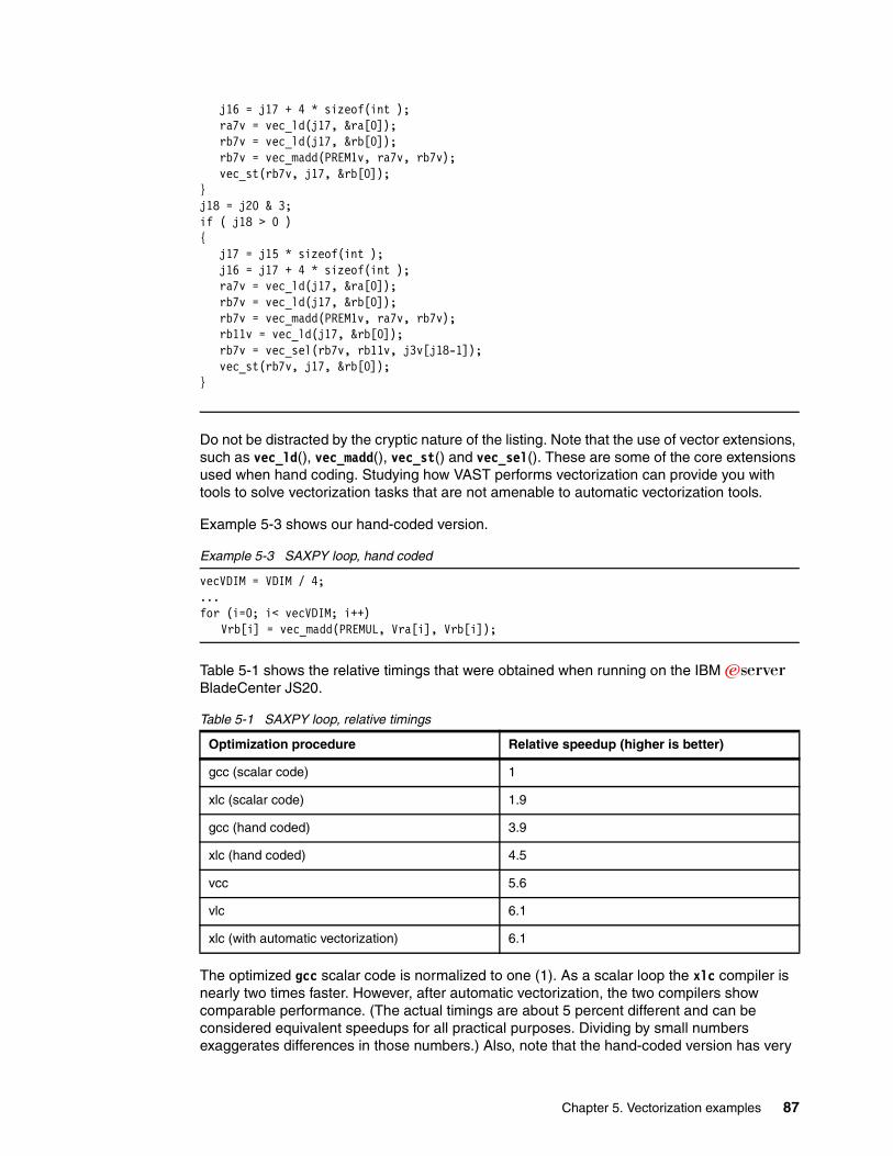
j16 = j17 + 4 * sizeof(int ); ra7v = vec_ld(j17, &ra[0]); rb7v = vec_ld(j17, &rb[0]); rb7v = vec_madd(PREM1v, ra7v, rb7v); vec_st(rb7v, j17, &rb[0]);}j18 = j20 & 3;if ( j18 > 0 ){ j17 = j15 * sizeof(int ); j16 = j17 + 4 * sizeof(int ); ra7v = vec_ld(j17, &ra[0]); rb7v = vec_ld(j17, &rb[0]); rb7v = vec_madd(PREM1v, ra7v, rb7v); rb11v = vec_ld(j17, &rb[0]); rb7v = vec_sel(rb7v, rb11v, j3v[j18-1]); vec_st(rb7v, j17, &rb[0]);}

Do not be distracted by the cryptic nature of the listing. Note that the use of vector extensions, such as vec_ld(), vec_madd(), vec_st() and vec_sel(). These are some of the core extensions used when hand coding. Studying how VAST performs vectorization can provide you with tools to solve vectorization tasks that are not amenable to automatic vectorization tools.

Example 5-3 shows our hand-coded version.

Example 5-3 SAXPY loop, hand coded

vecVDIM = VDIM / 4;...for (i=0; i< vecVDIM; i++)

Vrb[i] = vec_madd(PREMUL, Vra[i], Vrb[i]);

Table 5-1 shows the relative timings that were obtained when running on the IBM Eserver BladeCenter JS20.

Table 5-1 SAXPY loop, relative timings

The optimized gcc scalar code is normalized to one (1). As a scalar loop the xlc compiler is nearly two times faster. However, after automatic vectorization, the two compilers show comparable performance. (The actual timings are about 5 percent different and can be considered equivalent speedups for all practical purposes. Dividing by small numbers exaggerates differences in those numbers.) Also, note that the hand-coded version has very

Optimization procedure Relative speedup (higher is better)

gcc (scalar code) 1

xlc (scalar code) 1.9

gcc (hand coded) 3.9

xlc (hand coded) 4.5

vcc 5.6

vlc 6.1

xlc (with automatic vectorization) 6.1


few changes and receives most of the speedup. In fact, most of the changes needed are in setting up the vector variables, which are not shown.

If vector floating point is (theoretically) only two times faster than scalar floating point on the PowerPC 970, why are these speedups so much greater? Remember, not all gains are from vectorization. There can be additional gains from hiding load and store latencies.

5.2.2 Reduction loopThis loop is the generic reduction loop (for floating-point data) from BLAS. Example 5-4 shows the scalar version, which is also used for xlc vectorization.

Example 5-4 Reduction loop, scalar code

for (i=0; i< VDIM; i++){ sum += ra[i] ;}

Example 5-5 shows code that the vastcav optimizer generated.

Example 5-5 Reduction loop, vastcav code

*((float *)&sum2v) = sum;sum1v = vec_splat(sum2v, 0);j27 = VDIM;for ( j22 = 0; j22 < (j27 - 4 * 4) + 1; j22 += 4 * 4 ){ j24 = j22 * sizeof(int ); j23 = j24 + 4 * sizeof(int ); ra11v = vec_ld(j24, &ra[0]); ra12v = vec_ld(j24 + 16, &ra[0]); ra13v = vec_ld(j24 + 32, &ra[0]); ra14v = vec_ld(j24 + 48, &ra[0]); r13v = vec_add(r13v, ra11v); r15v = vec_add(r15v, ra12v); r16v = vec_add(r16v, ra13v); r17v = vec_add(r17v, ra14v);}if ( j22 ){ r13v = vec_add(r13v, r15v); r13v = vec_add(r13v, r16v); r13v = vec_add(r13v, r17v);}for ( ; j22 < (j27 - 4) + 1; j22 += 4 ){ j24 = j22 * sizeof(int ); j23 = j24 + 4 * sizeof(int ); ra11v = vec_ld(j24, &ra[0]); r13v = vec_add(r13v, ra11v);}j25 = j27 & 3;if ( j25 > 0 ){ j24 = j22 * sizeof(int ); j23 = j24 + 4 * sizeof(int ); ra11v = vec_ld(j24, &ra[0]); r19v = vec_sel(ra11v, r18v, j4v[j25-1]); r13v = vec_add(r13v, r19v);}


Example 5-6 shows the hand-coded version of the reduction loop. Note that details on variable declarations are excluded. You can view the entire source in the program, Exe1.c, that is included in the zipped file that accompanies this paper.

Example 5-6 Reduction loop, hand coded

vecVDIM = VDIM / 4;... Vsum = fzero;for (i=0; i< vecVDIM; i+=2){

Vsum1 = vec_add( Vra[i], Vra[i+1] );Vsum = vec_add( Vsum, Vsum1 );

}Vsum = vec_add( Vsum, vec_sld( Vsum, Vsum, 4 ) );Vsum = vec_add( Vsum, vec_sld( Vsum, Vsum, 8 ) );

Table 5-2 shows the relative timings that were obtained.

Table 5-2 Reduction loop, relative timings

Example 5-6 shows how scalar optimization with gcc can fall short on POWER hardware. Also, vectorization increased the performance of the hand-coded version. This result seems to be a reasonable based on the better scalar performance of xlc than gcc for the example.

5.2.3 Variation of the reduction loopThis version of the reduction loop is partially unrolled in a way that still allows vectorization. Example 5-7 shows the scalar version, which is also used for xlc vectorization. Note how the reduction is partitioned into four separate sections.

Example 5-7 Reduction loop variation, scalar code

for (i=0; i< VDIM/4; i++){ sum += ra[i] + ra[i + VDIM/4] + ra[i+ VDIM/2] + ra[i + 3*VDIM/4];}

Optimization procedure Relative speedup (higher is better)

gcc (scalar code) 1



vcc 10

vlc 11.2




Example 5-8 shows the code that the vastcav optimizer generated.

Example 5-8 Reduction loop variation, vastcav code

*((float *)&sum4v) = sum;sum3v = vec_splat(sum4v, 0);j34 = VDIM / 4;ra19v = vec_ld(0, &ra[VDIM/4]);ra22v = vec_ld(0, &ra[VDIM/2]);ra25v = vec_ld(0, &ra[(3*VDIM)/4]);for ( j29 = 0; j29 < (j34 - 4 * 2) + 1; j29 += 4 * 2 ){ j31 = j29 * sizeof(int ); j30 = j31 + 4 * sizeof(int ); ra15v = vec_ld(j31, &ra[0]); ra20v = vec_ld(j30, &ra[VDIM/4]); ra23v = vec_ld(j30, &ra[VDIM/2]); ra26v = vec_ld(j30, &ra[(3*VDIM)/4]); ra28v = vec_ld(j31 + 16, &ra[0]); ra29v = vec_ld(j30 + 16, &ra[VDIM/4]); ra31v = vec_ld(j30 + 16, &ra[VDIM/2]); ra33v = vec_ld(j30 + 16, &ra[(3*VDIM)/4]); ra16v = vec_perm(ra19v, ra20v, ra21v); ra17v = vec_perm(ra22v, ra23v, ra24v); ra18v = vec_perm(ra25v, ra26v, ra27v); r20v = vec_add(ra15v, ra16v); r20v = vec_add(r20v, ra17v);r20v = vec_add(r20v, ra18v); r21v = vec_add(r21v, r20v); ra30v = vec_perm(ra19v, ra29v, ra21v); ra32v = vec_perm(ra22v, ra31v, ra24v); ra34v = vec_perm(ra25v, ra33v, ra27v); r22v = vec_add(ra28v, ra30v); r22v = vec_add(r22v, ra32v); r22v = vec_add(r22v, ra34v); r23v = vec_add(r23v, r22v);}if ( j29 ) r21v = vec_add(r21v, r23v);for ( ; j29 < (j34 - 4) + 1; j29 += 4 ){ j31 = j29 * sizeof(int ); j30 = j31 + 4 * sizeof(int ); ra15v = vec_ld(j31, &ra[0]); ra20v = vec_ld(j30, &ra[VDIM/4]); ra16v = vec_perm(ra19v, ra20v, ra21v); ra23v = vec_ld(j30, &ra[VDIM/2]); ra17v = vec_perm(ra22v, ra23v, ra24v); ra26v = vec_ld(j30, &ra[(3*VDIM)/4]);ra18v = vec_perm(ra25v, ra26v, ra27v); r20v = vec_add(ra15v, ra16v);r20v = vec_add(r20v, ra17v); r20v = vec_add(r20v, ra18v); r21v = vec_add(r21v, r20v); ra19v = ra20v; ra22v = ra23v; ra25v = ra26v;}j32 = j34 & 3;if ( j32 > 0 ){


j31 = j29 * sizeof(int ); j30 = j31 + 4 * sizeof(int ); ra15v = vec_ld(j31, &ra[0]); ra20v = vec_ld(j30, &ra[VDIM/4]); ra16v = vec_perm(ra19v, ra20v, ra21v); ra23v = vec_ld(j30, &ra[VDIM/2]); ra17v = vec_perm(ra22v, ra23v, ra24v); ra26v = vec_ld(j30, &ra[(3*VDIM)/4]); ra18v = vec_perm(ra25v, ra26v, ra27v); r20v = vec_add(ra15v, ra16v);r20v = vec_add(r20v, ra17v); r20v = vec_add(r20v, ra18v); r25v = vec_sel(r20v, r24v, j5v[j32-1]); r21v = vec_add(r21v, r25v);}r20v = vec_sld(r21v, r21v, 8);r21v = vec_add(r21v, r20v);r20v = vec_sld(r21v, r21v, 4);r21v = vec_add(r21v, r20v);r21v = vec_add(r21v, sum3v);vec_ste(r21v, 0, &sum);


Example 5-9 Reduction loop variation, hand coded

vecVDIM = VDIM / 4;... Vsum = fzero;i2 = vecVDIM/4;i3 = vecVDIM/2;i4 = 3*vecVDIM/4;for (i=0; i< vecVDIM/4; i++, i2++, i3++, i4++){ Vsum1 = vec_add( Vra[i], Vra[i2] ); Vsum2 = vec_add( Vra[i3], Vra[i4] ); Vsum = vec_add( Vsum, Vsum1 ); Vsum = vec_add( Vsum, Vsum2 );} Vsum = vec_add( Vsum, vec_sld( Vsum, Vsum, 4 ) );Vsum = vec_add( Vsum, vec_sld( Vsum, Vsum, 8 ) );

Table 5-3 on page 92 summarized relative timings. The Relative speedup column is relative performance based on the code shown in the examples in this section. The Relative speedup when compared to previous version of the reduction loop column is timings relative to the loops discussed previously. Both values use the gcc compiled loop as the base timing case.


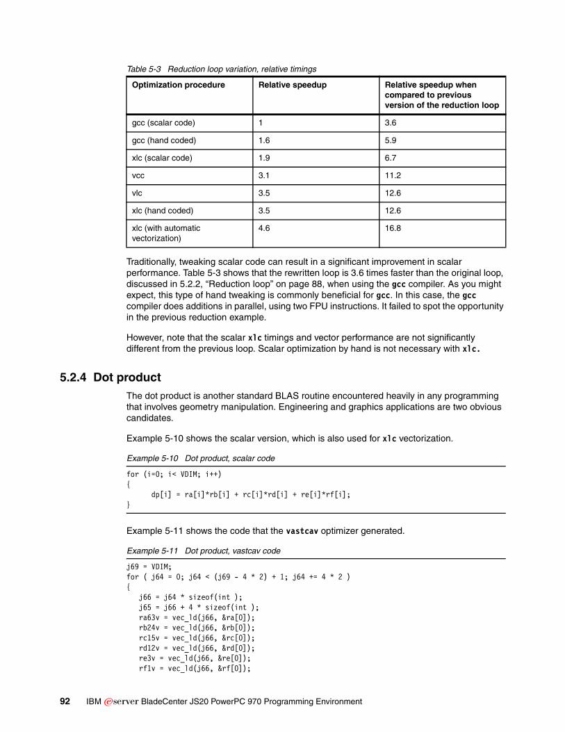
Table 5-3 Reduction loop variation, relative timings

Traditionally, tweaking scalar code can result in a significant improvement in scalar performance. Table 5-3 shows that the rewritten loop is 3.6 times faster than the original loop, discussed in 5.2.2, “Reduction loop” on page 88, when using the gcc compiler. As you might expect, this type of hand tweaking is commonly beneficial for gcc. In this case, the gcc compiler does additions in parallel, using two FPU instructions. It failed to spot the opportunity in the previous reduction example.

However, note that the scalar xlc timings and vector performance are not significantly different from the previous loop. Scalar optimization by hand is not necessary with xlc.

5.2.4 Dot productThe dot product is another standard BLAS routine encountered heavily in any programming that involves geometry manipulation. Engineering and graphics applications are two obvious candidates.

Example 5-10 shows the scalar version, which is also used for xlc vectorization.

Example 5-10 Dot product, scalar code

for (i=0; i< VDIM; i++){ dp[i] = ra[i]*rb[i] + rc[i]*rd[i] + re[i]*rf[i]; }

Example 5-11 shows the code that the vastcav optimizer generated.

Example 5-11 Dot product, vastcav code

j69 = VDIM;for ( j64 = 0; j64 < (j69 - 4 * 2) + 1; j64 += 4 * 2 ){ j66 = j64 * sizeof(int ); j65 = j66 + 4 * sizeof(int ); ra63v = vec_ld(j66, &ra[0]); rb24v = vec_ld(j66, &rb[0]); rc15v = vec_ld(j66, &rc[0]); rd12v = vec_ld(j66, &rd[0]); re3v = vec_ld(j66, &re[0]); rf1v = vec_ld(j66, &rf[0]);

Optimization procedure Relative speedup Relative speedup when compared to previous version of the reduction loop

gcc (scalar code) 1 3.6

gcc (hand coded) 1.6 5.9

xlc (scalar code) 1.9 6.7

vcc 3.1 11.2

vlc 3.5 12.6

xlc (hand coded) 3.5 12.6

xlc (with automatic vectorization)

4.6 16.8


ra64v = vec_ld(j66 + 16, &ra[0]); rb25v = vec_ld(j66 + 16, &rb[0]); rc16v = vec_ld(j66 + 16, &rc[0]); rd13v = vec_ld(j66 + 16, &rd[0]); re4v = vec_ld(j66 + 16, &re[0]); rf2v = vec_ld(j66 + 16, &rf[0]); r69v = vec_madd(ra63v, rb24v, r68v); r69v = vec_madd(rc15v, rd12v, r69v); dp1v = vec_madd(re3v, rf1v, r69v); vec_st(dp1v, j66, &dp[0]); r70v = vec_madd(ra64v, rb25v, r68v); r70v = vec_madd(rc16v, rd13v, r70v); dp2v = vec_madd(re4v, rf2v, r70v); vec_st(dp2v, j66 + 16, &dp[0]);}for ( ; j64 < (j69 - 4) + 1; j64 += 4 ){ j66 = j64 * sizeof(int ); j65 = j66 + 4 * sizeof(int );

ra63v = vec_ld(j66, &ra[0]); rb24v = vec_ld(j66, &rb[0]); rc15v = vec_ld(j66, &rc[0]); rd12v = vec_ld(j66, &rd[0]); re3v = vec_ld(j66, &re[0]); rf1v = vec_ld(j66, &rf[0]); r69v = vec_madd(ra63v, rb24v, r68v); r69v = vec_madd(rc15v, rd12v, r69v); dp1v = vec_madd(re3v, rf1v, r69v);

vec_st(dp1v, j66, &dp[0]);}j67 = j69 & 3;if ( j67 > 0 ){ j66 = j64 * sizeof(int ); j65 = j66 + 4 * sizeof(int ); ra63v = vec_ld(j66, &ra[0]); rb24v = vec_ld(j66, &rb[0]); rc15v = vec_ld(j66, &rc[0]); rd12v = vec_ld(j66, &rd[0]); re3v = vec_ld(j66, &re[0]); rf1v = vec_ld(j66, &rf[0]); r69v = vec_madd(ra63v, rb24v, r68v); r69v = vec_madd(rc15v, rd12v, r69v); dp1v = vec_madd(re3v, rf1v, r69v); dp3v = vec_ld(j66, &dp[0]); dp1v = vec_sel(dp1v, dp3v, j10v[j67-1]); vec_st(dp1v, j66, &dp[0]);}



Example 5-12 Dot product, hand coded

vecVDIM = VDIM / 4;... for (i=0; i< vecVDIM; i+=4){ Vsum1 = vec_madd( Vra[i], Vrb[i], fzero ); Vsum1 = vec_madd( Vrc[i], Vrd[i], Vsum1 ); Vdp[i] = vec_madd( Vre[i], Vrf[i], Vsum1 );

Vsum2 = vec_madd( Vra[i+1], Vrb[i+1], fzero ); Vsum2 = vec_madd( Vrc[i+1], Vrd[i+1], Vsum2 ); Vdp[i+1] = vec_madd( Vre[i+1], Vrf[i+1], Vsum2 );

Vsum3 = vec_madd( Vra[i+2], Vrb[i+2], fzero ); Vsum3 = vec_madd( Vrc[i+2], Vrd[i+2], Vsum3 ); Vdp[i+3] = vec_madd( Vre[i+3], Vrf[i+3], Vsum4 );

Vsum4 = vec_madd( Vra[i+3], Vrb[i+3], fzero ); Vsum4 = vec_madd( Vrc[i+3], Vrd[i+3], Vsum4 ); Vdp[i+2] = vec_madd( Vre[i+2], Vrf[i+2], Vsum3 );}

Table 5-4 summarizes the relative timings that were obtained.

Table 5-4 Dot product, relative timings

In terms of floating-point operations, a dot product is roughly three SAXPYs. Most linear algebra routines are built mainly of SAXPY operations. Variations in performance of simple loops are often due to the ratio of memory operations per SAXPY, regardless of the linear algebra routine. Loops doing more work can take advantage of better instruction scheduling, prefetching, and latency hiding.

5.2.5 Byte clampingCharacters (bytes) are the main data type that is manipulated in bioinformatics and data compression algorithms. Digital signal processing also relies heavily on fixed-point calculations. VMX hardware provides eight times the peak performance for loops that manipulate character data.

Example 5-13 on page 95 shows a loop which does single-byte manipulation and includes if-tests (branching). The resulting array is clamped between two values. (This is a crude form of band-pass filtering in digital signal processing.) You can use similar coding techniques in

Optimization procedure Relative speedup

gcc (scalar code) 1




vcc 3.5

vlc 3.7



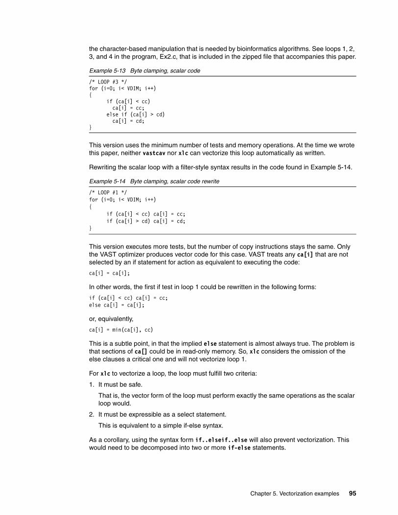
the character-based manipulation that is needed by bioinformatics algorithms. See loops 1, 2, 3, and 4 in the program, Ex2.c, that is included in the zipped file that accompanies this paper.

Example 5-13 Byte clamping, scalar code

/* LOOP #3 */for (i=0; i< VDIM; i++){ if (ca[i] < cc) ca[i] = cc; else if (ca[i] > cd) ca[i] = cd;}

This version uses the minimum number of tests and memory operations. At the time we wrote this paper, neither vastcav nor xlc can vectorize this loop automatically as written.

Rewriting the scalar loop with a filter-style syntax results in the code found in Example 5-14.

Example 5-14 Byte clamping, scalar code rewrite

/* LOOP #1 */for (i=0; i< VDIM; i++){ if (ca[i] < cc) ca[i] = cc; if (ca[i] > cd) ca[i] = cd;}

This version executes more tests, but the number of copy instructions stays the same. Only the VAST optimizer produces vector code for this case. VAST treats any ca[i] that are not selected by an if statement for action as equivalent to executing the code:

ca[i] = ca[i];

In other words, the first if test in loop 1 could be rewritten in the following forms:

if (ca[i] < cc) ca[i] = cc;else ca[i] = ca[i];

or, equivalently,

ca[i] = min(ca[i], cc)

This is a subtle point, in that the implied else statement is almost always true. The problem is that sections of ca[] could be in read-only memory. So, xlc considers the omission of the else clauses a critical one and will not vectorize loop 1.

For xlc to vectorize a loop, the loop must fulfill two criteria:

1. It must be safe.

That is, the vector form of the loop must perform exactly the same operations as the scalar loop would.

2. It must be expressible as a select statement.

This is equivalent to a simple if-else syntax.

As a corollary, using the syntax form if..elseif..else will also prevent vectorization. This would need to be decomposed into two or more if-else statements.


So, rewriting the loop to fulfill both vectorization criteria for xlc results in the code shown in Example 5-15.

Example 5-15 Byte clamping, final scalar rewrite

/* LOOP #4 */for (i=0; i< VDIM; i++){ if (ca[i] < cc) ca[i] = cc; else ca[i] = ca[i] ; if (ca[i] > cd) ca[i] = cd; else ca[i] = ca[i] ; }

The else statements in Example 5-15 are unnecessary when using scalar instructions. They would never be included in a scalar loop, because they just waste time. However, for the xlc compiler, these statements indicate that all ca[] elements will be written during execution. Thus, the xlc vectorizer can vectorize this loop using the VMX select function.

All of these loops write back into the tested array. The alternative approach of preserving ca[] and writing results into a new array cb[] from ca[] makes this loop almost five times slower; Loop 1 is four times slower and the results would be incorrect in practice. Reusing ca[] evidently reduces or eliminates a memory bottleneck.

Of course, the fastest scalar version is loop 3, because it eliminated wasted logical and memory operations present in the other loops. So, loop 3 is the basis for timings.

For loop 1, Example 5-16 shows the code that the vastcav optimizer generated.

Example 5-16 Byte clamping, vascav code for LOOP #1

*((unsigned char *)&cc2v) = cc; cc1v = vec_splat(cc2v, 0); *((unsigned char *)&cd2v) = cd; cd1v = vec_splat(cd2v, 0); for ( j1 = 0; j1 < (1024 - 16) + 1; j1 += 16 ) { j3 = j1 * sizeof(char ); j2 = j3 + 16 * sizeof(char ); cb1v = vec_ld(j3, &cb[0]); cb1v = vec_max(cb1v, cc1v); cb1v = vec_min(cb1v, cd1v); vec_st(cb1v, j3, &cb[0]); }


For loop 4, Example 5-17 shows the code that the vastcav optimizer generated.

Example 5-17 Byte clamping, vascav code for LOOP #4

*((unsigned char *)&cc6v) = cc;cc5v = vec_splat(cc6v, 0);*((unsigned char *)&cd6v) = cd;cd5v = vec_splat(cd6v, 0);*((unsigned char *)&cc8v) = cc;cc7v = vec_splat(cc8v, 0);*((unsigned char *)&cd8v) = cd;cd7v = vec_splat(cd8v, 0);for ( j15 = 0; j15 < (1024 - 16) + 1; j15 += 16 ) {

j17 = j15 * sizeof(char ); j16 = j17 + 16 * sizeof(char ); cf1v = vec_ld(j17, &cf[0]); c3v = vec_cmpgt(cc7v, cf1v); c1v = c3v; cf1v = vec_sel(cf1v, cc5v, c1v); c3v = vec_cmpgt(cf1v, cd7v); c2v = c3v; cf1v = vec_sel(cf1v, cd5v, c2v); vec_st(cf1v, j17, &cf[0]);}

Notice that the vastcav optimizer uses the select function (vec_sel) in the code that it generates to vectorize loop 4 but uses maximum (vec_max) and minimum (vec_min) functions to vectorize loop 1.

Example 5-18 shows our hand-coded version, which can be found in HVEx2.c.

Example 5-18 Byte clamping, hand coded

/* LOOP #5 */vecVDIM = VDIM / 4;... for (i=0; i< CvecVDIM; i++){ mask1 = vec_cmplt( Vca[i], Vcc ); mask2 = vec_cmpgt( Vca[i], Vcd ); Vca[i] = vec_sel( Vca[i], Vcc, mask1 ); Vca[i] = vec_sel( Vca[i], Vcd, mask2 );}


Table 5-5 shows the relative timings that were obtained.

Table 5-5 Byte clamping, relative timings

The coding example variations in Ex2.c and HVEx2.c are worth studying. All of them give the same result, but depending on the coding approach, the performance can vary by two times (whether in scalar or vector mode). This difference illustrates that hand tuning can still have an effect on vector performance in loops with branching. The base case taken for the gcc scalar timing is the fastest of the 4 loops, loop 3. The optimized timings (regardless of loop number) are all measured relative to this one. The VAST tool with the xlc compiler seems the best overall, though the actual timings differ by only by a few hundredths of a second.

5.2.6 SummaryThe best way to convert code to use vectorization instructions is to use one of the automatic vectorization tools, vastcav (via vcc or vlc) or xlc. These tools are not only the fastest way to vectorize code, they invariably provide the best performance gain.

Optimization procedure Relative speedup

xlc (scalar code of loop #3) 0.65

gcc (scalar code of loop #3) 1


xlc (with automatic vectorization on loop #4) 16.4


vcc 20.5

vlc 27.3


Chapter 6. A case study

This chapter describes the process of introducing vectorization into a scalar application known as POV-Ray.

6


6.1 Introducing vector code in your applicationThis chapter guides you step-by-step through the process of porting a scalar code into faster vector code using the vector instruction set. Vectorization can improve the performance for those applications that makes use of three-dimensional (3D) graphics, image processing, audio compression, or other calculation-intense functions.

As an example, we have an application for tuning, POV-Ray, the persistence of vision Raytracer. POV-Ray is a high-quality, totally freeware tool for creating 3D graphics. In Figure 6-1 shows a scene that was rendered with POV-Ray. This scene is explicitly intended to generate CPU benchmarks.

Figure 6-1 Standard scene for CPU benchmarks using POV-Ray

To assist in your porting efforts, the official Web site for POV-Ray source code is:

http://www.povray.org/

The modified source code for POV-Ray, and also some other vector enabled applications, are available at:

http://www.ciri.upc.es/cela_pblade/


http://www.povray.org/

http://www.ciri.upc.es/cela_pblade/

6.1.1 Appropriate uses of vectorizationUnlike other SIMD environments, taking advantage of VMX does not require you to write assembly language programs, and it is quite easy to use. However, before you start writing vector code for your application, you should consider some issues.

It might not be practical or even possible to rewrite your entire program using vector code. There might be too much branching and jumps in memory to run quickly using vectorization. However, vectorization might be worth the effort to convert that 10 percent of your application that consumes 90 percent of the CPU. Vectorization can also be useful for routines that work with large amounts of data and for complex calculations. This type of vectorization means that just a little work applied to the right functions can result in large improvements in overall speed.

If a small number of your application’s functions are relevant to its performance, it is important to choose in a scientific way, not a best guess, as to which functions to optimize. Instead, make use of the profiling tools.

To identify those functions inside POV-Ray, we compiled it with the compiler option, -pg. This option forces the compiler to generate extra code to write profile information that is suitable for analysis by the program, gprof. Before looking at the profiling results of POV-Ray, we should emphasize that the time that it spends in every function depends on the kind of scene that it is trying to render. Table 6-1 shows the profiling of POV-Ray rendering the scene called benchmark.pov. Remember that these results could be completely different for scenes with other requirements and properties.

Table 6-1 POV-Ray profiling for benchmark.pov

The file benchmark.pov is included with all distributions of POV-Ray and is located in the scenes\advanced directory. You might also need an INI file, which sets the standard benchmarking options. That file is available at:

http://www.povray.org/download/benchmark.ini

Notice that most of the time (60 percent) is spent in the functions Noise and DNoise. These two functions are very similar. If we can improve the performance of one of them, it will be very easy to apply the same ideas in the other function.

The purpose of these two functions is to generate random numbers. It is not uncommon in computer graphics and modelling to want to use a random function to make imagery or geometry appear more natural looking. The real world is not perfectly smooth nor does it move or change in regular ways. The random function found in the math libraries of most programming languages is not always suitable, because it results in a discontinuous function. The problem then is to find a random or noisy function that changes smoothly. It turns out that there are other desirable characteristics, such as it being defined everywhere (both at large scales and at very small scales) and for it to be band limited, at least in a controllable way.

% time cumulative seconds self seconds No. of calls name

31.69 29133.06 29133.06 220265125 Noise

29.65 56388.74 27255.68 2407569565 DNoise

6.62 62473.68 6084.94 169525839 POVFPU_RunDefault

2.50 64774.17 2300.49 150615313 f_ridged_mf

2.47 67043.53 2269.36 1346438698 MInvTransPoint

2.14 69010.69 1967.16 679937945 Warp_EPoint

Chapter 6. A case study 101

http://www.povray.org/download/benchmark.ini

The most famous practical solution to this problem came from Ken Perlin back in the 1980s. Noise and DNoise are modified functions based on Ken Perlin’s noise function. The basic idea is to create a seeded random number series and smoothly interpolate between the terms in the series, filling-in the gaps if you like.

Now that we have identified those functions that consumes most of our CPU time, we need to analyze the code to see if we can vectorize the data types and algorithms.

6.1.2 Analyzing data typesThe Noise function evaluates the noise in a 3D point of the space. When we examine its header, it has a VECTOR as a parameter, and it returns a floating point:

float Noise( VECTOR EPoint, TPATTERN *TPat );

The VECTOR data type is just an array of three floats. We are trying to introduce vector code into our application, and there is already a VECTOR data type in use. Unfortunately, it is not a good idea to fit a POV-Ray VECTOR into VMX vector float.

The key to achieving greater performance from the vector unit it is to clearly understand the SIMD paradigm. The SIMD format takes a single operation and applies it to all the data in the vector. Implicit in this arrangement is that each element in the vector should have the same meaning. This arrangement allows you to apply the same operation to all the elements of the vector at the same time without worrying that the operation is inappropriate or wrong for some of them.

A vector whose elements are all of the same data type is called a uniform vector. Uniform vectors can be used with the VMX ABI without having to be selective about which elements are modified. Because the vector elements are identical in meaning, they can be treated identically over the course of the calculation. This identical nature allows you to realize true four (32-bit data types), eight (16-bit data types), or 16 (8-bit data types) fold speed increases from vectorization, because you do not have to waste time protecting parts of the vector from certain operations that might do the wrong thing.

If we want to apply this idea in POV-Ray, we should see if it is possible to work in parallel with the Noise function. Is there any kind of data dependency between different executions of the function? Can we calculate the noise for four vectors at a time? Noise() is called from several places. In parts of the program, it is called just one time. If that was always the case, vectorization possibly would not benefit the application. However, most of the time, the function is called inside a loop, such as the one shown in Example 6-1.

Example 6-1 Call to function Noise

for (i = 1; i < 8; i++){ temp[0]=EPoint[0]*lambda; temp[1]=EPoint[1]*lambda; temp[2]=EPoint[2]*lambda; value += omega * Noise(temp, TPat); lambda *= 2.0; omega *= 0.5;}

In this loop, Noise() is called once every iteration, with temp as a parameter, and stores its returning value in value. As you can see, temp is updated every iteration, but there is no dependence with the returning value of Noise() from the previous iteration. As sequential iterations of the loop are not dependent in each other, we can operate on multiple iterations of this loop in parallel.


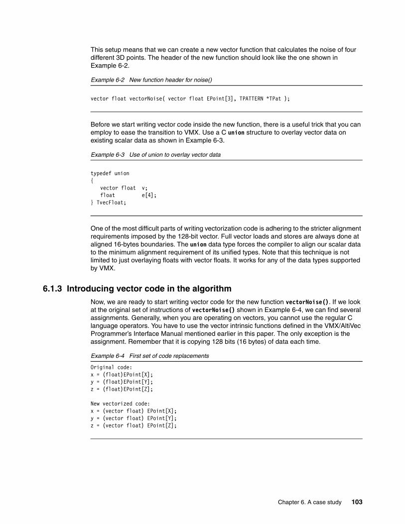
This setup means that we can create a new vector function that calculates the noise of four different 3D points. The header of the new function should look like the one shown in Example 6-2.

Example 6-2 New function header for noise()

vector float vectorNoise( vector float EPoint[3], TPATTERN *TPat );

Before we start writing vector code inside the new function, there is a useful trick that you can employ to ease the transition to VMX. Use a C union structure to overlay vector data on existing scalar data as shown in Example 6-3.

Example 6-3 Use of union to overlay vector data

typedef union{

vector float v;float e[4];

} TvecFloat;

One of the most difficult parts of writing vectorization code is adhering to the stricter alignment requirements imposed by the 128-bit vector. Full vector loads and stores are always done at aligned 16-bytes boundaries. The union data type forces the compiler to align our scalar data to the minimum alignment requirement of its unified types. Note that this technique is not limited to just overlaying floats with vector floats. It works for any of the data types supported by VMX.

6.1.3 Introducing vector code in the algorithmNow, we are ready to start writing vector code for the new function vectorNoise(). If we look at the original set of instructions of vectorNoise() shown in Example 6-4, we can find several assignments. Generally, when you are operating on vectors, you cannot use the regular C language operators. You have to use the vector intrinsic functions defined in the VMX/AltiVec Programmer’s Interface Manual mentioned earlier in this paper. The only exception is the assignment. Remember that it is copying 128 bits (16 bytes) of data each time.

Example 6-4 First set of code replacements

Original code:x = (float)EPoint[X];y = (float)EPoint[Y];z = (float)EPoint[Z];

New vectorized code:x = (vector float) EPoint[X];y = (vector float) EPoint[Y];z = (vector float) EPoint[Z];


Let us analyze the second set of instructions shown in Example 6-5. We need to do a comparison. VMX provides a complete set of vector comparison primitives and predicates. The result of the comparison operations is a vector of type boolean, that is used as a mask. In the scalar code, we want to know if the x point is greater than or equal to zero. If this is not true, we should subtract a constant from x. When we think about this as a vector, we are going to change the logic a bit. In vector coding and in some instances, it is less time consuming to do the conversion and not use it, than it is to spend time analyzing the code to see if the conversion should be done. With that in mind, in this case, it would be less time consuming to compute the result of both branches of the conditional instruction and then choose the right value.

Example 6-5 Second set of code replacements

Original code:tmp = (x >= 0) ? (int)x : (int)(x - 0.999999);

New vectorized code:faux = vec_sub( x, fcons1 );baux = vec_cmpge( x, fzero );faux = vec_sel( faux, x, baux );tmp = vec_cts( faux, 0 );

What’s going on here? It looks like a C instruction is being converted into four vector instructions. Remember that the C programming language allows us to write complex operations that involve several instructions, while vector manipulations are low-level operations that most of the time translates into just one machine instruction. And what are these new variables fzero and fcons1? These variables store constant values. The variable fzero is a vector float initialized with all 0.0 and fcons1 is initialized with 0.9999999. They should be declared at the beginning of the function.

In the first instruction we store the result of ‘x - 0.999999’ into the variable faux. Remember that we are probably not using all the elements of faux, but it’s faster to compute them than choose which one to compute and which one not. Next, we create the mask vector baux comparing every element of x with zero. This mask is used to choose between x and faux for every one of its components. Finally, we made a type conversion using vec_cts().

Note that VMX extensions do not automatically make type conversions. If we made an assignment between different types of vectors it will make a bit copy. For instance, the hexadecimal value 0x00000001 expressed as an integer is equal to 1, but expressed as a floating point number is a very small number, near zero. If you want to avoid this kind of problems you should explicitly use the appropriate vector instruction.

After we have finished with the conditional instruction, we move to the next set of instructions as shown in Example 6-6 on page 105. In this set, it is straight forward to convert the scalar instructions into vector instructions, because most of the scalar operations translate into one vector operation. By the way, in this set there are some other vector constants that you should define, imin, iFFF, ione, fone, and fthree.


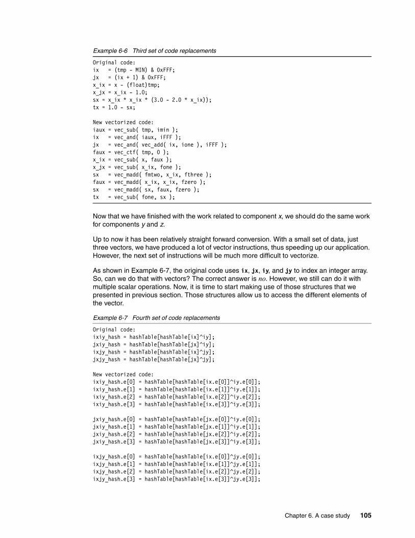
Example 6-6 Third set of code replacements

Original code:ix = (tmp - MIN) & 0xFFF;jx = (ix + 1) & 0xFFF;x_ix = x - (float)tmp;x_jx = x_ix - 1.0;sx = x_ix * x_ix * (3.0 - 2.0 * x_ix));tx = 1.0 - sx;

New vectorized code:iaux = vec_sub( tmp, imin );ix = vec_and( iaux, iFFF );jx = vec_and( vec_add( ix, ione ), iFFF );faux = vec_ctf( tmp, 0 );x_ix = vec_sub( x, faux );x_jx = vec_sub( x_ix, fone );sx = vec_madd( fmtwo, x_ix, fthree );faux = vec_madd( x_ix, x_ix, fzero );sx = vec_madd( sx, faux, fzero );tx = vec_sub( fone, sx );

Now that we have finished with the work related to component x, we should do the same work for components y and z.

Up to now it has been relatively straight forward conversion. With a small set of data, just three vectors, we have produced a lot of vector instructions, thus speeding up our application. However, the next set of instructions will be much more difficult to vectorize.

As shown in Example 6-7, the original code uses ix, jx, iy, and jy to index an integer array. So, can we do that with vectors? The correct answer is no. However, we still can do it with multiple scalar operations. Now, it is time to start making use of those structures that we presented in previous section. Those structures allow us to access the different elements of the vector.

Example 6-7 Fourth set of code replacements

Original code:ixiy_hash = hashTable[hashTable[ix]îy];jxiy_hash = hashTable[hashTable[jx]îy];ixjy_hash = hashTable[hashTable[ix]^jy];jxjy_hash = hashTable[hashTable[jx]^jy];

New vectorized code:ixiy_hash.e[0] = hashTable[hashTable[ix.e[0]]îy.e[0]];ixiy_hash.e[1] = hashTable[hashTable[ix.e[1]]îy.e[1]];ixiy_hash.e[2] = hashTable[hashTable[ix.e[2]]îy.e[2]];ixiy_hash.e[3] = hashTable[hashTable[ix.e[3]]îy.e[3]];

jxiy_hash.e[0] = hashTable[hashTable[jx.e[0]]îy.e[0]];jxiy_hash.e[1] = hashTable[hashTable[jx.e[1]]îy.e[1]];jxiy_hash.e[2] = hashTable[hashTable[jx.e[2]]îy.e[2]];jxiy_hash.e[3] = hashTable[hashTable[jx.e[3]]îy.e[3]];

ixjy_hash.e[0] = hashTable[hashTable[ix.e[0]]^jy.e[0]];ixjy_hash.e[1] = hashTable[hashTable[ix.e[1]]^jy.e[1]];ixjy_hash.e[2] = hashTable[hashTable[ix.e[2]]^jy.e[2]];ixjy_hash.e[3] = hashTable[hashTable[ix.e[3]]^jy.e[3]];


jxjy_hash.e[0] = hashTable[hashTable[jx.e[0]]^jy.e[0]];jxjy_hash.e[1] = hashTable[hashTable[jx.e[1]]^jy.e[1]];jxjy_hash.e[2] = hashTable[hashTable[jx.e[2]]^jy.e[2]];jxjy_hash.e[3] = hashTable[hashTable[jx.e[3]]^jy.e[3]];

As you see, we are accessing the vector, element by element, repeating the instructions for each one of its components. This repetition means that we are not improving our algorithm by reducing the number of operations. In fact, it is worst. We are moving data from the vector unit to the scalar unit. We are introducing some delays that deteriorates the performance of our application. Moreover, the next set of code shown in Example 6-8 is not much better.

Example 6-8 Fifth set of code replacements

Original code:mp = &RTable[hashTable[ixiy_hashîz]&0xFF) << 1];sum = txty*tz*(mp[1] + mp[2]*x_ix + mp[4]*y_iy + mp[6]*z_iz;

New vectorized code:mp0 = &RTable[hashTable[ixiy_hash.e[0]îz.e[0]]&0xFF) << 1];mp1 = &RTable[hashTable[ixiy_hash.e[1]îz.e[1]]&0xFF) << 1];mp2 = &RTable[hashTable[ixiy_hash.e[2]îz.e[2]]&0xFF) << 1];mp3 = &RTable[hashTable[ixiy_hash.e[3]îz.e[3]]&0xFF) << 1];ss.v = vec_madd( txty.v, tz.v, fzero ); // txty*tzsum.e[0] = ss.e[0]*(mp0[1]+mp0[2]*x_ix+mp0[4]*y_iy+mp0[6]*z_iz.e[0]);sum.e[1] = ss.e[1]*(mp1[1]+mp1[2]*x_ix+mp1[4]*y_iy+mp1[6]*z_iz.e[1]);sum.e[2] = ss.e[2]*(mp2[1]+mp2[2]*x_ix+mp2[4]*y_iy+mp2[6]*z_iz.e[2]);sum.e[3] = ss.e[3]*(mp3[1]+mp3[2]*x_ix+mp3[4]*y_iy+mp3[6]*z_iz.e[3]);

In this set of instructions, we are also accessing the hash table, and we use the returning value to index RTable. RTable is a floating point array of pseudorandom numbers. Also, note that for every value that we want to compute we need to access to four nonconsecutive values of RTable.

As you can see, this code is not likely to use vector instructions. Thus, it was not a good idea to introduce vector code in a function that generates random numbers.


6.1.4 ConclusionsIf we analyze the new function vectorNoise(), we can differentiate the main parts. In the first part, we did not have any problem making good use of VMX extensions. However, in the second part, we are hardly using any vector instructions. In fact, we end up moving some data from the vector unit to the scalar unit. So, is it really worthy to use VMX in this function? Table 6-2 shows the result of our efforts.

Table 6-2 Performance comparison

We have improved the Noise function. Now it is working just over two times faster, and we still are not taking advantage of all the capabilities of VMX. As we have said before, VMX programming cannot be used everywhere. Our purpose was not to show you an easy vectorization example, but to show you a complex example illustrating how to deal with vector code.

Finally, remember that if you want to optimize your code, the introduction of vector instructions should be the last step in the process. Keep in mind these tips:

� Do not waste your time optimizing all your code.

Use a profiler to identify those functions that consumes most of the CPU time.

� Make sure that you are using the right algorithm.

The performance difference between a good algorithm and a bad one can be several orders of magnitude.

� Arrange your data as uniform vectors.

It is better to have a structure with several vectors than a vector of several structures. It is more easy to work in parallel if adjacent data has the same meaning.

� Optimize memory usage.

The speed of a function could be limited by the speed of the CPU or by the speed of the system bus. If your algorithm is limited by the speed of the system bus, the function runs at the same speed regardless you vectorize your code. Before doing any vectorization in your code, you should improve the memory usage. For example, try to reduce the amount of data used in your algorithm or structure your program to do more work with the data loaded into the caches.

� Improve the software pipelining of your algorithm.

If you want your processor work at full performance, make sure that it is plenty of independent operations to avoid dependencies. Unroll your loop four or more vectors at a time. Do not unroll the loop completely, because this will load too much the instruction cache, which may hurt the performance.

� Make wise use of the cache instructions.

VMX allow us to load data from main memory do the L1 cache, meaning that you can ask for data before using it.

Function Time/interation Total Time Speedup

Original Noise() 52.80 5279868 1

vectorNoise() 25.63 2563420 2.06


Appendix A. Code listings

This appendix lists the contents of the source zipped file, vmxcode.zip, that is available with this paper.

Code examples� Ex1.c

Example 1 source code - Scalar C floating point test cases

� Ex2.c

Example 2 source code - Scalar C integer and character test cases

� HVEx1.c

Hand-coded VMX extensions added to Ex1.c

� HVEx2.c

Hand-coded VMX extensions added to Ex2.c

� VACEx1.lst

Output C code from VAC autoSIMDization for Ex1.c

� VACEx2.lst

Output C code from VAC autoSIMDization for Ex2.c

� VEx1.c

Ouput C code from Vast preprocessor for Ex1.c

� VEx2.c

Ouput C code from Vast preprocessor for Ex2.c

� Ex1.lst

Message output from Vast preprocessor for Ex1.c

� Ex2.lst


A


� Ex1.lst


� Ex2.lst


� Ex1.tim

timing results for Example 2 loops

� Ex2.tim

timing results for Example 3 loops

� Makefile.vast

Makefile for generating scalar binaries and VMX binaries with VAST and gcc

� Makefile.xlc

Makefile for generating VMX binaries with xlc autoSIMDization

� Makefile.hv

Makefile for generating VMX binaries from hand-coded examples

� Ex1.csh

script to run Example 2 binaries for timing

� Ex2.csh

script to run Example 3 binaries for timing

Code loops from Toronto Labs VAC test suite

Arithmetic Ops on Floatsadd256_1add256_2sub256_1test_rt_ub_add_1

Arithmetic Ops on 1-byte, 2-byte, 4-byte Integersmul_16_16_16mul_16_16_16_unsignedmul_16_16_32mul_16_16_32_unsignedmul_16_32_32mul_16_32_32_unsignedmul_32_16_32mul_32_16_32_unsignedmul_32_32_32mul_32_32_32_unsignedshort_1short_2short_3short_add_invariantshort_add_litshort_sel_1test_privatization_1test_privatization_2test_privatization_3vtest_l2_s1_d2_dto4_db0.8_r0_b0_0


vtest_l2_s1_d2_dto4_r0_b0_0vtest_l2_s1_d2_r0_b0.3_0vtest_l2_s1_d4_r0_b0.3_0vtest_l2_s2_d2_dto4_r0_b0_0vtest_l3_s1_d4_r0_b0.3_0vtest_l4_s1_d2_dto4_r0_b0_0vtest_l4_s1_d2_r0_b0.3_0vtest_l4_s1_d4_r0_b0.3_0vtest_l4_s2_d2_dto4_db0.8_r0_b0_0vtest_l4_s2_d2_dto4_db0.8_r0_b0_rtime_ilu_0vtest_l4_s2_d2_r0.3_b0.3_0vtest_l4_s2_d4_r0.3_b0.3_0vtest_l4_s4_d2_r0.3_b0.3_0vtest_l4_s4_d4_r0.3_b0.3_0vtest_l4_s4_d4_r0_b0_0vtest_l4_s4_d4_r0_b0_1vtest_l4_s4_d4_r0_b0_2vtest_l4_s4_d4_r0_b0.3_0vtest_l4_s4_d4_r0_b0_3vtest_l4_s4_d4_r0_b0_4vtest_l4_s4_d4_r0_b0_5vtest_l4_s4_d4_r0_b0_6vtest_l4_s4_d4_r0_b0_7vtest_l4_s4_d4_r0_b0_8vtest_l4_s4_d4_r0_b0_9vtest_l6_s1_d2_r0_b0.3_0vtest_l6_s1_d4_r0_b0.3_0vtest_l8_s4_d2_r0.3_b0.3_0vtest_l8_s4_d4_r0.3_b0.3_0

Memory alignment with data type conversionconvert_misalign_16to32convert_misalign_sint32to16_2convert_misalign_sint32to16_3convert_misalign_sint32to16_4convert_misalign_sint32to16_5convert_misalign_sint32to16convert_misalign_sint32to16_rt_1convert_misalign_sint32to16_rt_2convert_misalign_sint32to16_rt_3convert_misalign_sint32to16_rt_4convert_misalign_sint32to16_rt_5

Data type conversionconvert_sint16_to_32convert_sint16_to_64convert_sint32_to_16convert_sint32_to_8convert_uint16_to_32_rtconvert_uint32_to_16_rtconvert_uint32_to_8_rtconvert_uint8_to_32_rt

Matrix multiplicationmatmul_1

Appendix A. Code listings 111

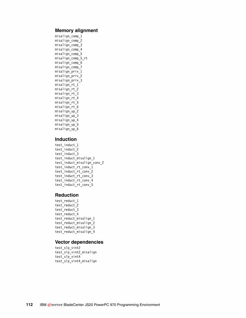
Memory alignmentmisalign_comp_1misalign_comp_2misalign_comp_3misalign_comp_4misalign_comp_5misalign_comp_5_rtmisalign_comp_6misalign_comp_7misalign_priv_1misalign_priv_2misalign_priv_3misalign_rt_1misalign_rt_2misalign_rt_3misalign_rt_4misalign_rt_5misalign_rt_6misalign_up_2misalign_up_3misalign_up_4misalign_up_5misalign_up_6

Inductiontest_induct_1test_induct_2test_induct_3test_induct_misalign_1test_induct_misalign_conv_2test_induct_rt_conv_1test_induct_rt_conv_2test_induct_rt_conv_3test_induct_rt_conv_4test_induct_rt_conv_5

Reductiontest_reduct_1test_reduct_2test_reduct_3test_reduct_4test_reduct_misalign_1test_reduct_misalign_2test_reduct_misalign_3test_reduct_misalign_4

Vector dependenciestest_slp_vint2test_slp_vint2_misaligntest_slp_vint4test_slp_vint4_misalign


Appendix B. Porting from Apple OS X

Porting AltiVec or VMX code from Apple OS X gcc to Linux gcc on a IBM Eserver BladeCenter JS20 is a somewhat trivial task. You need to understand the subtle differences in syntax between the two implementations of gcc.

Compiler FlagsIn order for gcc to recognize vector instructions while compiling with Linux gcc on a IBM Eserver BladeCenter JS20, the flags -maltivec and -mabi=altivec must be specified. These compiler flags enable the built-in functions and macros required to access the VMX instruction set.

Alternatively, if IBM xlc is going to be used, -qarch=ppc970, -qenablevmx and -qaltivec allow architecture specific instructions to be generated, thus enabling VMX for xlc.

In addition to compiler flags, the file altivec.h must be included in each source file that uses vector instructions. The inclusion of altivec.h is implicit when using gcc on OS X or with IBM xlc.

Initialization SyntaxThere are several differences in syntax that are troublesome when porting AltiVec/VMX code from OS X to Linux.

� Initialization Syntax

The primary difference is in declaration statements for vectors. The gcc compiler on Linux does not support initializing vectors using parentheses ( ). It only uses curly braces { }. For example, the following is allowed under OS X, but not Linux:

vector int single = (vector int)(1); /*{1,1,1,1}*/vector int quad = (vector int)(1,1,1,1); /*(1,1,1,1)*/

B


The following is allowed under both OS X and Linux:

vector int single = {1}; /*{1,0,0,0}*/vector int quad = {1,1,1,1}; /*{1,1,1,1}*/

This brings up a significant point: gcc on Linux only supports the initialization of vectors through curly braces { }. This is not typically used by code written natively on OS X. Most OS X code initializes vectors with parenthesis. Under OS X, this creates a complete vector containing the initialized value. However, when compiled by gcc on Linux, only the first element of the vector would be initialized. If you had the following code originally written for OS X, the result would return {2,2,2,2} with gcc on OS X, and {2,1,1,1} with gcc on Linux.:

vector int single = (vector int)(1); /*{1,1,1,1}*/vector int quad = (vector int)(1,1,1,1); /*(1,1,1,1)*/vector int result;

result = vec_add(single, quad);

� Passing literal vectors as parameters

All overloaded VMX functions are implemented in gcc on Linux through macros. As a result, when passing literal vectors to a function, they must be wrapped in parenthesis ( ). For example:

result = vec_msum(v1, ((vector int){1,4,6,3,5,8,3,9}), (vector int){0});

� Using vector long is deprecated

Another slight difference is that gcc on Linux treats vector long and vector int as different data types. Data should be specified as int instead of long as long is considered deprecated when using VMX to avoid data type incompatibility.

Best PracticesWhen writing VMX code that is to be portable for both OS X and Linux using the gcc compiler, it is best to write as though the target is Linux. VMX code developed on Linux almost always functions as expected on OS X.

The key is to be explicit when initializing and using vectors. For example, if initially developing in OS X, always declare vectors as vector int quad = {1,1,1,1}; and not vector int single = (vector int)(1); because that would be syntactically correct only in OS X and not Linux.

Using compiler predefined macros enable greater portability between OS X and Linux. While using gcc on OS X, the following relevant predefined macros are defined by the compiler when the flag -faltivec is used:

__APPLE____ALTIVEC__

Compiling on Linux with gcc and with the -maltivec flag, produces the following:

__LINUX____ALTIVEC__


IBM Visual AgePreliminary experimentation with IBM xlc demonstrates that xlc handles VMX instructions similarly to the OS X gcc compiler. As mentioned previously, the compiler flags -qarch=ppc970, -qenablevmx, and -qaltivec are required to enable VMX. The IBM xlc performs exactly the same as OS X gcc with the initialization of vectors as well as supports most of the vector operations.

ReferencesFor information about the Apple AltiVec Velocity Engine, see:

http://developer.apple.com/hardware/ve

Appendix B. Porting from Apple OS X 115

http://developer.apple.com/hardware/ve

Appendix C. Additional material

This Redpaper refers to additional material that can be downloaded from the Internet as described below.

Locating the Web materialThe Web material associated with this Redpaper is available in softcopy on the Internet from the IBM Redbooks Web server. Point your Web browser to:

ftp://www.redbooks.ibm.com/redbooks/REDP-3890

Alternatively, you can go to the IBM Redbooks Web site at:

ibm.com/redbooks

Select Additional materials and open the directory that corresponds with the Redpaper form number, REDP-3890.

Using the Web materialThe additional Web material that accompanies this Redpaper includes the following files:

File name Descriptionvmxcode.zip A zipped file of sample VMX code

C


ftp://www.redbooks.ibm.com/redbooks/



System requirements for downloading the Web materialWe recommend the following system configuration:

Hard disk space: 5 MB minimumOperating System: AIX or LinuxProcessor: PowerPC 970 or 970FXMemory: 256 MB

How to use the Web materialCreate a subdirectory (folder) on your workstation, and unzip the contents of the Web material zipped file into this folder.


Related publications

The publications listed in this section are considered particularly suitable for a more detailed discussion of the topics covered in this Redpaper.

IBM RedbooksFor information about ordering these publications, see “How to get IBM Redbooks” on page 120. Note that some of the documents referenced here may be available in softcopy only.

� The POWER4 Processor Introduction and Tuning Guide, SG24-7041

� PMaC Benchmarking on Three POWER4 Platforms, REDP-3724

� IBM eServer BladeCenter Configuration Tips, TIPS-0454

Other publicationsThese publications are also relevant as further information sources:

� PowerPC Microprocessor Family: AltiVec Technology Programming Environments Manual

– http://www-306.ibm.com/chips/techlib/techlib.nsf/techdocs/FBFA164F824370F987256D6A006F424D

– http://www.technonics.com/publications

– http://www.freescale.com/files/32bit/doc/ref_manual/ALTIVECPIM.pdf

� Compiler Reference - XL C/C++ Advanced Edition V7.0 for AIX, SC09-7887

� Programming Guide - XL C/C++ Advanced Edition V7.0 for AIX, SC09-7888

� Compiler Reference - XL C/C++ Advanced Edition V7.0 for Linux, SC09-7942

� Programming Guide - XL C/C++ Advanced Edition V7.0 for Linux, SC09-7943

� VAST-C/AltiVec, Automatic C Vectorizer for Motorla AltiVec

http://www.crescentbaysoftware.com/docs/vastcav.pdf


http://www-306.ibm.com/chips/techlib/techlib.nsf/techdocs/FBFA164F824370F987256D6A006F424D

http://www.crescentbaysoftware.com/docs/vastcav.pdf

http://www.technonics.com/publications

http://www.freescale.com/files/32bit/doc/ref_manual/ALTIVECPIM.pdf

Online resourcesThese Web sites and URLs are also relevant as further information sources:

� GNU Compiler Collection

http://gcc.gnu.org

� VAST Automatic C Vectorizer

http://www.crescentbaysoftware.com

� PowerPC Training


� PowerPC 970 Manuals and Datasheets


How to get IBM RedbooksYou can search for, view, or download Redbooks, Redpapers, Hints and Tips, draft publications, and Additional materials, as well as order hardcopy Redbooks or CD-ROMs, at this Web site:

ibm.com/redbooks

Help from IBMIBM Support and downloads

ibm.com/support

IBM Global Services

ibm.com/services




http://www.ibm.com/support/

http://www.ibm.com/support/

http://www.ibm.com/services/

http://www.ibm.com/services/

http://gcc.gnu.org

http://www.crescentbaysoftware.com



Index

Numerics128-bit 10–11, 14, 36, 38, 10316-bit 10, 20, 36, 38, 44, 55, 59, 61, 63, 84, 10232-bit 10–11, 14, 16–17, 19–20, 29, 36, 38, 48–49, 54–56, 59, 61, 63, 68, 84, 86, 10264-bit 1, 4, 9–11, 14–15, 17–18, 20, 24, 27–29, 31, 44, 56, 688-bit 10, 36, 38, 44, 49, 59, 61, 63, 84, 102

AAccess Concentrators/DSLAMS 37Address space register (ASR) 15AltiVec 3, 14, 35, 49, 54–55, 61, 70–71, 103Application Binary Interface (ABI) 24, 27–31, 70Array number processing 37ATLAS 55automatic vectorization 54–55, 58, 70, 72–73, 80, 85, 87autoSIMDization 39

BBasic Linear Algebra Subroutines (BLAS) 86, 92BLAS 88Byte clamping 94

CCommunications 37Condition register (CR) 14Configuration registers 14Crescent Bay Software 58

DData address breakpoint register (DABR) 16Data address register (DAR) 15Data encryption

RSA 37Data storage interrupt status register (DSISR) 15Decrementer register (DEC) 16Dot product 92

EEcho cancellation 37Extended precision 11

FFast Fourier Transforms 55Floating-point registers (FPRs) 14Floating-point status and control register (FPSCR) 14

Gglobal offset table (GOT) 27

© Copyright IBM Corp. 2005. All rights reserved.

gprof tool 101

HHardware implementation-dependent register 0 16Hardware implementation-dependent register 1 16Hardware implementation-dependent register 4 16Hardware implementation-dependent register 5 16High bandwidth data communication 37High-fidelity audio 37High-precision CAD 37

IIEEE 754 Standard for Binary Floating-Point Arithmetic 9Instruction address breakpoint (IABR) 16interelement operation 47intraelement operation 47

JJPEG 37

KKen Perlin’s noise function 102

LLink Register (LR) 28

MMachine State Register (MSR) 17Machine state register (MSR) 14Machine status save/restore register 0 (SRR0) 15Machine status save/restore register 1 (SRR1) 15Memory management registers 15Miscellaneous registers 16Monitor mode control registers (MMCR0, MMCR1, MMCRA) 16Motorola 3, 71MPEG-1 37MPEG-2 37MPEG-4 37

NNeural algorithms 37

OOpenGL 37Operating Environment Architecture (OEA) 14

PPerformance monitor counter registers 16

121

Performance monitor registers 16Pipelined execution 23POV-Ray 100PowerPC

data types 10PowerPC 970-specific registers 16PowerPC instructions 19

add 20addi 20–21addo 20A-form 19b 28ba 28bc 28bcctr 28bclr 28bdnz 21beq 45B-form 19bl 28bla 28cmpwi 45D-form 19DS-form 19dss 43, 46dssall 43, 46dst 43dstst 43, 45eieio 20fmadd 21hrfid 17I-form 19isync 20ld 11lfdu 21lvx 42lwarz 20lwz 11, 20, 45MD-form 19MDS-form 19M-form 19mfspr 14mtmsr 14, 17mtmsrd 17mtspr 14, 21mtvscr 47mulwo 20rfi 14rfid 17sc 14, 17SC-form 19stfdu 21vaddsbs 47vaddshs 47vaddsws 47vaddubs 47vadduhs 47vadduws 47vctsxs 47vctuxs 47

vmhaddshs 47vmhraddshs 47vmsumshs 47vmsumuhs 47vperm 49vpkshss 47vpkshus 47vpkswss 47vpkswus 47vpkuhus 47vpkuwus 47vsubsbs 47vsubshs 47vsubsws 47vsububs 47vsubuhs 47vsubuws 47vsum2sws 47vsum4sbs 47vsum4shs 47vsum4ubs 47vsumsws 47XFL-form 19X-form 19XFX-form 19XL-form 19XO-form 19XS-form 19

Pragmas 79printf() 61Problem state 12Processor ID register (PIR) 16Processor version register (PVR) 15

QQuickDraw 37

RReal-time continuous speech 37Redbooks Web site 120

Contact us xiReduced Instruction Set Computer (RISC) 3Reduction loop 88Register sets 12Registers

Address space register (ASR) 15Condition register (CR) 14Configuration registers 14Data address registers (DAR) 15Data storage interrupt status register (DSISR) 15Decrementer register (DEC) 16Floating-point registers (FPRs) 14Floating-point status and control register (FPSCR) 14general-purpose registers 9, 12–14, 25, 28, 33, 40Hardware implementation-dependent register 0 16Hardware implementation-dependent register 1 16Hardware implementation-dependent register 4 16Hardware implementation-dependent register 5 16Instruction address breakpoint (IABR) 16


Link Register (LR) 28Machine state register (MSR) 14, 17Machine status save/restore register 0 (SRR0) 15Machine status save/restore register 1 (SRR1) 15memory management 15Miscellaneous registers 16Monitor mode control registers (MMCR0, MMCR1, MMCRA) 16Performance monitor counter registers 16Performance monitor registers 16PowerPC 970-specific registers 16PowerPC sets 12Processor ID register (PIR) 16Processor version register (PVR) 15Sampled data address register (SDAR) 16Sampled instruction address register (SIAR) 16Special purpose registers (SPRs) 14Storage description register (SDR1) 15Supervisor-level registers 14Time base (TB) 16User-level registers 14Vector Multimedia eXtensions (VMX) 26Vector registers (VRs) 14Vector status and control register (VSCR) 14

Return values of functions 33RISC 19

SSampled data address register (SDAR) 16Sampled instruction address register (SIAR) 16Saturation 47Saturation clamping 38SAXPY 86scanf() 61Sequential execution 23Special purpose registers (SPRs) 14Speech recognition 37sscanf() 63Stack pointer 30Storage description register (SDR1) 15Superscalar 22, 24Supervisor-level registers 14

TTable of Contents (TOC) 27Time base (TB) 16

UUseful pragmas 79User-level registers 14

Vva_list 31VAST 55, 58, 84–85vastcav 58Vector data types 59Vector keywords 60

__pixel 60

__vector 60bool 60pixel 60vector 60

Vector Multimedia eXtensions (VMX) ix, 1, 4–6, 9, 17, 26, 31, 33–34, 39, 54–58, 71, 84–85, 94, 101–103, 107, 126

C extensions 61compiler options 70registers 26

Vector registers (VRs) 14Vector save/restore register (VRSAVE) 14Vector status and control register (VSCR) 14Vectorization reports 80Video conferencing 37Virtual reality 37Viterbi acceleration 37Voice over IP (VoIP) 37Voice/sound processing 37VRML 37

Index 123

®

INTERNATIONAL TECHNICALSUPPORTORGANIZATION

BUILDING TECHNICAL INFORMATION BASED ON PRACTICAL EXPERIENCE

IBM Redbooks are developed by the IBM International Technical Support Organization. Experts from IBM, Customers and Partners from around the world create timely technical information based on realistic scenarios. Specific recommendations are provided to help you implement IT solutions more effectively in your environment.

For more information:ibm.com/redbooks

RedpaperIBM Eserver BladeCenter JS20PowerPC 970 Programming Environment

PowerPC 970 microprocessors

Vector Multimedia Extensions (VMX)

Optimization and performance considerations

This Redpaper gives a broad understanding of the programming environment of the IBM PowerPC 970 microprocessor that is implemented in the IBM Eserver BladeCenter JS20.

It also provides information on how to take advantage of the Vector Multimedia Extensions (VMX) execution unit found in the PowerPC 970 to increase the performance of applications in 3D graphics, modelling and simulation, digital signal processing, and others.

Back cover




powerpc 970 programming environment - ibm · pdf fileiv ibm eserver bladecenter js20 powerpc...

Documents