power rating of photovoltaic modules using a new outdoor ... · i would like to thank dr. narcio f....

Power Rating of Photovoltaic Modules Using a

New Outdoor Method

by

Meena Gupta Vemula

A Thesis Presented in Partial Fulfillment of the Requirements for the Degree

Master of Science in Technology

Approved April 2012 by the Graduate Supervisory Committee:

Govindasamy Tamizhmani, Chair

Narcio F. Macia Bradley Rogers

ARIZONA STATE UNIVERSITY

May 2012

i

ABSTRACT

Photovoltaic (PV) modules are typically rated at three test conditions: STC

(standard test conditions), NOCT (nominal operating cell temperature) and

Low E (low irradiance). The current thesis deals with the power rating of

PV modules at twenty-three test conditions as per the recent International

Electrotechnical Commission (IEC) standard of IEC 61853-1. In the

current research, an automation software tool developed by a previous

researcher of ASU-PRL (ASU Photovoltaic Reliability Laboratory) is

validated at various stages. Also in the current research, the power rating

of PV modules for four different manufacturers is carried out according to

IEC 61853-1 standard using a new outdoor test method. The new outdoor

method described in this thesis is very different from the one reported by a

previous researcher of ASU-PRL. The new method was designed to

reduce the labor hours in collecting the current-voltage (I-V) curves at

various temperatures and irradiance levels. The power matrices for all the

four manufacturers were generated using the I-V data generated at

different temperatures and irradiance levels and the translation

procedures described in IEC 60891 standard.

All the measurements were carried out on both clear and cloudy days

using an automated 2-axis tracker located at ASU-PRL, Mesa, Arizona.

The modules were left on the 2-axis tracker for 12 continuous days and

ii

the data was continuously and automatically collected for every two

minutes from 6 am to 6 pm. In order to obtain the I-V data at wide range of

temperatures and irradiance levels, four identical (or nearly identical)

modules were simultaneously installed on the 2-axis tracker with and

without thermal insulators on the back of the modules and with and

without mesh screens on the front of the modules.

Several issues related to the automation software were uncovered and the

required improvement in the software has been suggested. The power

matrices for four manufacturers have been successfully generated using

the new outdoor test method developed in this work. The data generated

in this work has been extensively analyzed for accuracy and for

performance efficiency comparison at various temperatures and irradiance

levels.

iii

DEDICATION

I would like to dedicate this work to my parents, VenuGopal Setty and

Kalavathi, and to my fiancé Preetham Kumar Duggishetti. It is only

because of their support and encouragement that I can stand here today.

iv

ACKNOWLEDGEMENTS

I would like to express my utmost gratitude to Dr. Govindasamy

Tamizhmani for his enthusiastic support, guidance, and encouragement

throughout this work. His insight and expertise in PV technologies was

invaluable. I have learned much under his guidance and he has given me

opportunities to expand my knowledge base. I am truly fortunate to have

worked with him.

I would like to thank Dr. Narcio F. Macia and Dr. Bradley Rogers for

their interest, valuable input, and suggestions, and for serving as

members of the Thesis committee.

I would like to thank all students and staff of PRL for their support.

In particular, I thank Mr. James Gonzales and Arseniy Voropayev for their

technical help and guidance. Also, I would like to thank my fellow students

who have helped me for this thesis: Kartheek Koka, Sai Ravi Vasista

Tatapudi, Lorenzo Tyler, Faraz Ebneali, and all students of PRL.

I would also like to thank Marcos Fernandes and Karen Paghasian

for giving me their extensive research work data.

Finally, words alone cannot express the thanks I owe to my family

for their support and encouragement. Without them and a blessing from

the one above, it would never have been possible.

v

TABLE OF CONTENTS

Page

LIST OF TABLES .................................................................................... viii

LIST OF FIGURES ..................................................................................... x

CHAPTER

1. INTRODUCTION ................................................................................... 1

2. LITERATURE REVIEW ......................................................................... 4

2.1 Translation Procedures of IEC 60891 .............................................. 6

2.1.1 Procedure 1. The first ................................................................. 6

2.1.2 Procedure 2. .............................................................................. 7

2.1.3 Procedure 3. .............................................................................. 8

2.1.4 Procedure 4. Procedure 4 .......................................................... 9

3. METHODOLOGY ................................................................................ 11

3.1 Collecting the Data for Baseline .................................................... 13

3.2 Calibration of the Meshes .............................................................. 18

3.3 Linearity Check .............................................................................. 20

3.4 Collecting the Data for Final Analysis ............................................ 20

3.5 Translation Procedure ................................................................... 24

3.5.1 Procedure 1. Chapter 2 ............................................................ 25

3.5.2 Procedure 2. Chapter 2 ............................................................ 30

3.6 Power Matrix .................................................................................. 32

4. RESULTS AND DISCUSSIONS .......................................................... 34

4.1 Automation Software ..................................................................... 34

vi

CHAPTER Page

4.2 Collecting the Baseline Data .......................................................... 35

4.3 Mesh Calibration for Transmittance ............................................... 37

4.4 Data Collection on Two Axis Tracker ............................................. 38

4.5 Parameters .................................................................................... 49

4.6 Validation of Automation Software ................................................. 51

4.7 Validation of First Two Procedures of IEC 60891 .......................... 51

4.8 Comparison of Power Matrices of a Manufacturer at Different

Conditions ............................................................................................... 53

4.9 Power Matrix Generated Using Procedure 3 ................................. 61

4.10 Comparison of Efficiencies of a Manufacturer at Different

Conditions ............................................................................................... 62

4.11 Comparison of Four Manufacturers ............................................. 67

4.12 Advantages and Disadvantages of Automation Software ............ 72

4.12.1 Single-step automation. ......................................................... 72

4.12.2 Multiple-step automation. ....................................................... 73

4.12.3 Hybrid method (manual + automation). .................................. 73

4.13 Comparison between Four Procedures of IEC 60891 ................. 76

4.14 Power Temperature Coefficient ................................................... 79

5. CONCLUSIONS AND RECOMMENDATIONS .................................... 81

5.1 Conclusions ................................................................................... 81

5.1.1 Number of Days Required for Data Collection – ...................... 81

5.1.2 Procedure selection – .............................................................. 81

vii

CHAPTER Page

5.1.3 Software Validation – ............................................................... 82

5.1.4 New Outdoor Test Method – .................................................... 82

5.1.5 Comparison of power temperature coefficient at various

irradiance levels – ............................................................................. 83

5.1.6 Comparison of Different Manufacturers – ................................ 84

5.2 Recommendation .......................................................................... 84

REFERENCES ........................................................................................ 86

viii

LIST OF TABLES

Table Page

1. Power Matrix as per IEC 61853-1 .......................................................... 2

2. Mesh Transmittance Calibration of Set 1 ............................................. 38

3. Mesh Transmittance Calibration of Set 2 ............................................. 38

4. Power Matrix for hypothetical 100 W module ...................................... 50

5. Comparison of Manual and Automation results of mono crystalline

module (Paghasian, 2010). ..................................................................... 51

6. Comparison between Procedure 1 and Procedure 2 for M2 considering

four modules for 12 days ......................................................................... 52

7. Comparison of a power matrices generated for 4 modules of

Manufacturer 3 using procedure 1 between 1 day and 6 days ................ 54


Manufacturer 3 using procedure 1 between 1 day and 12 days .............. 54


Manufacturer 3 using procedure 1 between 6 days and 12 days ............ 55

10. Comparison of idle and calculated power for 1 day data of four

modules for M3 ........................................................................................ 56

11. Comparison of idle and calculated power for 6 days data of four

modules for M3 ........................................................................................ 57

12. Comparison of idle and calculated power for 12 days data of four

modules for M3 ........................................................................................ 57

ix

Table Page

13. Comparison of idle and calculated power for 1 day data of one module

of M3 ....................................................................................................... 59

14. Comparison of idle and calculated power for 6 days data of one

module of M3 ........................................................................................... 59

15. Comparison of idle and calculated power for 12 days data of one

module of M3 ........................................................................................... 60

16. Comparison of Power between 4 modules data to 1 module data for

12 days of M3 manufacturer .................................................................... 61

17. Comparison of multiple steps automation to hybrid method for M3

using procedure 2 .................................................................................... 75

18. Comparison of module rated power at STC with the powers calculated

using automation software and hybrid method ........................................ 76

19. Comparison of four procedures of IEC 60891 from this project

perspective .............................................................................................. 77

x

LIST OF FIGURES

Figure Page

1. Curve Selection in Procedure 3 ............................................................. 8

2. Curve Selection for Procedure 4 .......................................................... 10

3. Thermocouple positions on the backside of PV module ...................... 12

4: The process flow of the entire project .................................................. 14

5. Four different modules data at STC ..................................................... 15

6. Series and Shunt resistances in a Solar Cell [8] .................................. 16

7. Series Resistance effect on Solar Cell [8] ........................................... 17

8. Shunt Resistance effect on Solar Cell [8] ............................................ 18

9. Setup of one set (four similar modules of one manufacturer) on two Axis

Tracker platform and they are connected Multi-curve tracer ................... 21

10. Backside view of two modules with and without insulation on a two

axis tracker .............................................................................................. 22

11. IV curve ............................................................................................. 22

12. Procedure to obtain temperature coefficients for Procedure1............ 25

13. Steps involved in obtaining Rs of IEC 60891 procedure 1 ................. 26

14. Three Curves at different Irradiances and constant temperature to

determine “Rs” (for Procedure 2 it’s “a” and “Rs’ ”) .................................. 27

15. After determining “Rs” (for Procedure 2 it’s “a” and “Rs’ ”); the

translated curves and original curve merge on each other ...................... 27

16. Steps involved in obtaining k of IEC 60891 procedure 1 ................... 28

xi

Figure Page

17. Three curves at different Temperatures and constant Irradiance, to

determine “k” ........................................................................................... 29

18. After determining “k,” the translated curves and original curve merge

on each other........................................................................................... 29

19. Procedure to obtain temperature coefficients for Procedure 2........... 30

20. Steps involved in obtaining a, Rs’ of IEC 60891 procedure 2............. 31

21. Steps involved in obtaining k’ of IEC 60891 procedure 2 .................. 32

22. Automation Software Main Page ....................................................... 35

23. Conventional Baseline Procedure – An example ............................... 36

24. Baseline I-V Curves of four modules of Manufacturer A at STC ....... 37

25. Steps used to cleanup and obtain quality data to use as input for the

automation software ................................................................................ 39

26. Figure showing the raw irradiance & module temperature data

obtained on 24th Nov 2011 (partially cloudy day; fall season)– with 4

modules, in which 2 are covered with mesh screens & the other 2 modules

with thermal insulation as explained in the experimental setup section ... 41

27. Figure showing the raw irradiance & module temperature data

obtained on 19th Oct’11 (clear sunny day; fall season) – with 4 modules,

in which two are covered with mesh screens & the other two modules with

thermal insulation as explained in the experimental setup section .......... 42

28. Data collected on 19th Oct.11 from Module 3 ..................................... 43

29. I-V Curve when there is a passing cloud ........................................... 44

xii

Figure Page

30. IV Curve taken when there is no passing cloud ................................. 45

31. Single day Data set from Module 1 of M2, showing curves on a cloudy

day ........................................................................................................... 46

32. Isc Vs Irradiance data without clearing the irregular data ................... 47

33. Isc/Irradiance Vs Irradiance data without clearing the irregular data .. 47

34. Isc Vs Irradiance data after cleaning up the irregular data that was

shown in Figure 24 .................................................................................. 48

35. Isc/Irradiance Vs Irradiance data after removing the outlier data in

Figure 25 ................................................................................................. 48

36. Power Matrix generated with procedure for four modules of M1using

12 days .................................................................................................... 62

37. Efficiency of a manufacturer (4 modules and 12 days) at four different

temperatures ........................................................................................... 63

38. Efficiency of a manufacturer (4 modules and 1 day) at four different

temperatures ........................................................................................... 65


temperatures ........................................................................................... 65


temperatures ........................................................................................... 66

41. Comparison of Efficiencies at different Irradiance levels and at

constant temperature of 15 C ................................................................. 67

xiii

Figure Page







45. Comparison of Efficiencies at constant Irradiance @ 1000 W/m2 and

different temperature ............................................................................... 72

46 – Comparison of the power temperature coefficients at various

irradiance levels for M1 manufacturer ..................................................... 79

1

Chapter 1

INTRODUCTION

Photovoltaic (PV) modules are typically rated at standard test

conditions (STC) of 1000 W/m2 and 25C temperature and air mass 1.5

global spectrum. However, the PV modules operate in the field at various

temperatures, irradiance, and spectral conditions. Recognizing this issue,

the IEC (International Electro technical Commission) has released a new

standard, IEC 61853-1, which explains that the module needs to be rated

according to 23 element power matrix, which is shown in Table 1.

The module temperatures and irradiances vary vastly owing to

location, altitude, hour of the day, season of the year, and sun intensity.

As such, the power matrix is required to help analyze/decide on the

number of modules to be present in the installation to drive a certain load

under different climatic and variation factors.

The performance of the module depends on the Irradiance and

temperature factors; it is very important to have an idea about how the

power produced from PV modules changes with these factors before

building a system. This can be understood as the irradiance influences

the module’s short circuit current directly and open circuit voltage

logarithmically. At the same point, the module temperature has more

effect on open circuit voltage. As the power is voltage times current, these

factors affect the power extensively.

2

The IEC has released another standard, IEC 60891, which was

released before IEC 61853-1 and it delineates three procedures which can

be used in translating from one curve to the other.

Table 1. Power Matrix as per IEC 61853-1

The previous researchers of Arizona State University’s

Photovoltaics Reliability Laboratory (ASU-PRL) have validated the

translation procedures of IEC 60891 by comparing it with real-time results

[6].

The initial part of the project was to generate an “automation

version” for the IEC 60891 procedures and the power matrix of IEC

61853-1. The three procedures of this standard were automated along

with the other program, “baseline procedure” (which is not a part of the

standard, but its results were used in the procedures). This part of the

project was performed by the previous researcher of ASU PRL [1] who

Irradiance (W/m2)

Module Temperature (°C)

15 25 50 75

1100 NA 1 2 3

1000 4 5 6 7

800 8 9 10 11

600 12 13 14 15

400 16 17 18 NA

200 19 20 21 NA

100 22 23 NA NA

3

developed the software and extensive help with troubleshooting and

improving the software were offered by the current researcher. This part of

the project included:

Deciding upon the requirements of the software,

Explaining the functionality of the procedures,

Testing and validating the software.

For data analysis, this project was conducted on Poly crystalline PV

modules. This part of the project can be divided into the following stages:

Selecting four manufacturers

Selecting four similar or nearly-identical modules of same model

from each manufacturer

Checking the linearity of the devices

Calibrating the meshes used in this project

Placing each set (four modules of each manufacturer) on the two

axis tracker with different setup – using mesh and insulation

Connecting modules to the multi curve tracer to collect the data

Collecting the data for twelve days at different irradiances and

temperatures from sun rise to sun set

Generating the power matrix according to IEC-61853-1 using IEC-

60891 procedures

Comparing three power matrices generated using the three

procedures of IEC-60891

Comparing the power matrices generated.

4

Chapter 2

LITERATURE REVIEW

One of the most important PV standards being developed by the

IEC/TC82/WG2 Committee (International Electro technical Commission/

Technical Committee 82/Working Group 2) is the IEC 61853 standard

titled “Photovoltaic Module Performance Testing and Energy Rating” [5].

This standard is composed of four parts:

IEC 61853-1: It describes requirements for evaluating PV module

performance in terms of power (watts) rating over a range of

irradiances and temperatures.

IEC 61853-2: It describes test procedures for measuring the effect

of varying angle of incidence and sunlight spectra, the estimation of

module temperature from irradiance, ambient temperature, and

wind speed.

IEC 61853-3: It describes the calculations for PV module energy

(watt-hours) ratings.

IEC 61853-4: It describes the standard time periods and weather

conditions that can be utilized for the energy rating calculations.

The first part of the standard titled “IEC 61853-1: Irradiance and

Temperature Performance Measurements and Power Rating” was

published in January of 2011. This standard specifies the performance

measurements of PV modules at 23 different sets of temperature and

5

irradiance conditions, as shown in Table 1, using either a solar simulator

(indoor) or the natural sunlight (outdoor). There are several indoor and

outdoor techniques possible and many of those techniques are allowed by

this standard. For successful implementation of this standard, these

techniques need to be repeatable in the same laboratory and reproducible

between different laboratories over a period of time. The power rating

measurements at various temperatures and irradiance levels are more

challenging under prevailing outdoor conditions as compared to controlled

indoor conditions. This study report deals with two rounds of outdoor

measurements and results:

Round-1: 12 days measurements are used to find the power

matrix

Round-2: 6 days measurements are considered to compare the

results with 12 days

Round-3: 1 day measurements are considered to compare the

results with 12 days

All the measurements were carried out at the air mass levels less

than 2.5 and matched reference cell technologies to minimize and neglect

the spectral mismatch error.

This report discusses the process carried out using the Automatic

Two Axis tracker with a different set up. The data was analyzed using the

four translation procedures of IEC 60891 to obtain the performance

6

characteristics at different test conditions. This chapter will explain the

mathematical equations behind each procedure.

The four translation procedures are used to translate from one

curve to any other target curve. These procedures [4] can also be used to

translate the measured data into the data points on the P matrix.

2.1 Translation Procedures of IEC 60891

2.1.1 Procedure 1. The first procedure is used to translate a single

measured I-V characteristic to select temperature and irradiance or test

conditions by using equations (1) and (2).

I2 = I1 + Isc [(G2/G1) – 1] + α (T2 – T1) --------------- (1)

V2 = V1 – Rs (I2 – I1) – k I2 (T2 – T1) + β (T2 – T1) --------------- (2)

Where:

I1 (A) and V1 (V) are coordinates of the measured I-V curve

I2 (A) and V2 (V) are the coordinates of the translated I-V curve

G1 (W/m2) is the irradiance measured with the primary reference cell

G2 (W/m2) is the irradiance at desired conditions in the matrix

T1 (C) is the module temperature

T2 (C) is the desired temperature in the matrix

Isc (A) is the measured short circuit current of the test specimen for

measured I-V curve

Rs () is the internal resistance of the test module

7

k (/k) is the curve correction factor derived from measured

conditions

α (A/k) and β (V/k) are temperature coefficients of Isc and Voc

respectively

These temperature coefficients are calculated at the target irradiances.

IEC 60891 describes how to determine the other parameters Rs and k,

which is demonstrated in the Methodology chapter.

2.1.2 Procedure 2. IEC 60891 Procedure 2, is similar to Procedure 1 with

additional correction parameters required. The following equations are

used to achieve the current and voltage coordinates of the translated

curve.

I2 = I1 * (1 + αrel * (T2 – T1)) * G2/G1 ------- (3)

V2 = V1 + Voc1 * ( βrel * (T2 – T1) + a * ln (G2/G1)) – R’s * (I2 – I1) – k’ * I2 *

(T2 – T1) ------- (4)

I1 (A) and V1 (V) are coordinates of the measured I-V curve

I2 (A) and V2 (V) are the coordinates of the translated I-V curve

G1 (W/m2) is the irradiance measured with the primary reference cell

G2 (W/m2) is the irradiance at desired conditions in the matrix

T1 (C) is the module temperature

T2 (C) is the desired temperature in the matrix

Voc (V) is the measured open circuit voltage of the test specimen for

measured I-V curve

8

a is the irradiance correction factor for open circuit voltage which is

linked with the diode thermal voltage D of the p-n junction and the

number of cell ns serially connected in the module

Rs’ () is the internal resistance of the test specimen

k' (/k) is the temperature coefficient of the series resistance Rs’

αrel (1/k) and βrel (1/k) are the current and voltage temperature

coefficients at STC (Standard Test Conditions)

IEC 60891 describes how to determine the other parameters a, Rs’ and k’

and is shown in the Methodology chapter.

2.1.3 Procedure 3. The third procedure is derived from linear interpolation

or extrapolation of 3 curves from measured I-V values that were taken

from our PV module. The irradiance (Gn) and temperatures (Tn) are also

considered since they have a direct linearly effect on the current and

voltage output. The values to be considered are at (Ga, Ta), (Gb, Tb) and

(Gc, Tc) and they need to be selected as shown in Figure 1.

Figure 1. Curve Selection in Procedure 3

(gm,tm) (ga,ta)

(gc,tc)

(gb,tb)

(gn,tn)

9

G3 = G1 + a ⋅ (G2 −G1)

T3 = T1 + a ⋅ (T2 − T1)

a= (G3-G1)/(G2-G1)

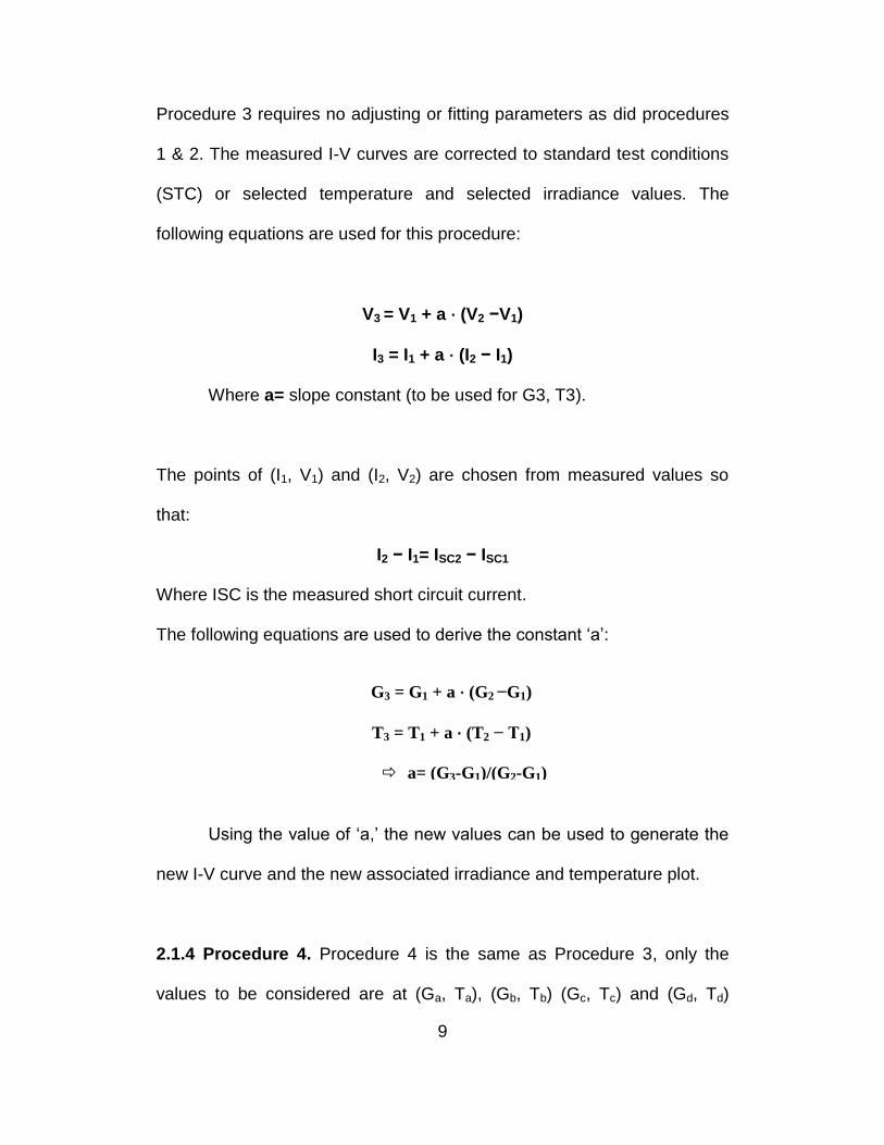
Procedure 3 requires no adjusting or fitting parameters as did procedures

1 & 2. The measured I-V curves are corrected to standard test conditions

(STC) or selected temperature and selected irradiance values. The

following equations are used for this procedure:

V3 = V1 + a ⋅ (V2 −V1)

I3 = I1 + a ⋅ (I2 − I1)

Where a= slope constant (to be used for G3, T3).

The points of (I1, V1) and (I2, V2) are chosen from measured values so

that:

I2 − I1= ISC2 − ISC1

Where ISC is the measured short circuit current.

The following equations are used to derive the constant ‘a’:

Using the value of ‘a,’ the new values can be used to generate the

new I-V curve and the new associated irradiance and temperature plot.

2.1.4 Procedure 4. Procedure 4 is the same as Procedure 3, only the

values to be considered are at (Ga, Ta), (Gb, Tb) (Gc, Tc) and (Gd, Td)

10

shown in the Figure 2 and the final (Gn,Tn) are calculated in similar

manner. Initially (Gx,Tx) and (Gy, Ty) are calculated and they are used to

generate the (Gn,Tn) data.

Figure 2. Curve Selection for Procedure 4

(Gn,Tn)

(Ga,Tb)

(Gb,Tb)

(Gc,Tc)

(Gd,Td)

(Gy,Ty) (Gx,Tx)

11

Chapter 3

METHODOLOGY

The project was planned for different test processes. They are:

Indoor Processes – Using Solar Simulator for the data collection.

Outdoor Process – Using real Solar power for the data collection.

The test began for the indoor process, but it was not continued. It

had few setup problems for which there was need of some new

equipment. With the present set up we had temperature differences seen

between different locations on the module at the time of testing. The

module was initially cooled/ heated to particular temperature and then the

data was collected as the temperature increased/ decreased towards the

room temperature. The various points at which the temperature was

collected are shown in Figure 3. Where T1 is temperature at the center

and T2 is temperature at the end of the module. As the temperature

difference between T1 and T2 was around 10 C, it was not acceptable for

the research, so different experiments were tried out to maintain the same

temperature throughout the module, but it was not feasible with the

methods followed. As it was not good for research to continue with the first

procedure, the test was performed only with the second method.

12

Figure 3. Thermocouple positions on the backside of PV module

The second method was to perform the same test outdoors. The

outdoor measurements can be taken in different methods –

(i) Fixed tilt

(ii) Single Axis Tracker

(iii) Two Axis Tracker

a) Manual Two Axis Tracker – for which we need to check the

sun direction and face the tracker towards it manually.

b) Automatic Two Axis Tracker – this one has a sensor and a

controller which tracks the sun throughout the day.

In this project, an automatic two-axis tracker was used. This project

was planned to use four different manufacturers and four similar modules

from each manufacturer. The similarity of the modules was checked by

comparing the equivalence of the temperature coefficients and different

T1

T2

13

parameters at STC conditions, which will be discussed later in this

chapter. The process flow of this project is shown in figure 4. The project

has various stages in it as shown in figure 4. Each stage is explained

briefly in this chapter.

3.1 Collecting the Data for Baseline

The data was collected at different temperatures, starting from a

temperature as low as 15C to a maximum temperature of 75 C and

irradiance from lowest to the highest irradiance values using different

meshes. The data was collected at different irradiances – ~100 W/m2

(using ~10% T meshes), ~200 W/m2 (using ~20% T meshes), ~400 W/m2

(using ~40% T meshes), ~600 W/m2 (using ~60% T meshes), ~800 W/m2

(using ~80% T meshes) and ~1000 W/m2 (without any mesh) {where T is

transmittance}.

14

Figure 4: The process flow of the entire project

15

To collect data at lower temperatures, the modules were cooled to

a very low temperature in an environmental chamber and then placed on

the manual two-axis tracker. The tracker was set in such a way that the

modules exactly faced the sun. The set up included two reference cells,

test module, IV curve tracer and a computer connected to it to collect the

data, thermo couples to collect the module, ambient temperature, and

meshes.

The data was collected from a low temperature to a high

temperature in steps of approximately 2C with different meshes.

This data was analyzed to find the temperature coefficients which

were to be used further to analyze the main data. Four modules of a

manufacturer are declared as similar; when the temperature coefficients

are approximately equal and IV (current – voltage) curve data at STC for

all four modules needed to overlap as shown in Figure 5.

Figure 5. Four different modules data at STC

Voltage (V)

Isc (A)

16

The temperature coefficients of any two modules need not be equal

even if the modules belong to same model/ manufacturer/technology. The

temperature coefficients vary due to the variations in the parasitic

resistances. These variations in the parasitic resistances are due to the

manufacturing process.

The parasitic resistances affect the power, fill factor, and efficiency

of that module. The types of parasitic resistive losses are the series

resistance and shunt resistance. The circuit schematic of a solar cell

considering these two types of resistances is shown in Figure 6.

Figure 6. Series and Shunt resistances in a Solar Cell [8]

A module should have a low series resistance and high shunt

resistance. The IV curve of a module will be affected by high series

resistance and low shunt resistance. The series resistance effect can be

seen at the higher irradiance levels and as the series resistance increases

the curve looks like a triangle. In figure 7, there are two curves shown, one

is a typical I-V curve shown in red color. If the series resistance is

17

increased for the same module and I-V curve is collected, it will be as the

blue curve shown in figure 7.

Figure 7. Series Resistance effect on Solar Cell [8]

Both series and shunt resistances affect the module’s IV curve. The

shunt resistance effect is seen at low irradiance levels whereas series

resistance effect is seen at higher irradiance levels. Figure 8 shows two

curves (blue curve with low shunt resistance and the red curve with higher

shunt resistance). The IV curve will be affected as the shunt resistance

decreases.

This study is performed to see how these resistances affect the

module’s power under different conditions in the 23 element power matrix.

Chapter 4 discusses the 23 element power matrix of different

manufacturers and thereby compares the effects of the above mentioned

18

factors on the PV modules in terms of power and efficiency. It also

discusses how this study is helpful for an installer or a consumer in

deciding the module for installation depending on the working conditions

of the place.

Figure 8. Shunt Resistance effect on Solar Cell [8]

3.2 Calibration of the Meshes

There are two sets of meshes used for this project:

Set 1 – Meshes used to collect the baseline data.

Set 2 – Meshes used to collect 12 days/4 days data which is the

main required data for this research.

19

The meshes used for baseline measurements are approximately

10%T, 20%T, 40%T and 60%T, and they are calibrated prior to the

measurements.

The meshes that are used to collect the data from four modules on

two axis tracker are approximately 25%T and 65%T meshes. These

meshes need to be calibrated to know exactly how much irradiance is

transmitted through them.

Reference cell could have been covered with these meshes to

calculate the transmittance directly. But as the meshes were not uniform

throughout, reference cell being very small in size comparatively, the

irradiance cannot be predicted accurately. The sensitivity to the irradiance

transmitted was very high, leading it to be unusable in this procedure. This

was proved by an ASU PTL previous researcher’s master thesis study

(Paghasian, 2010). The thesis study tells us that “to calibrate a mesh, it

needs to be placed on top of the Module and the reference cell should be

left uncovered” (p. #). It also says that “the mesh should be placed at least

1.5” above the module to have uniform effect” (p. 97). Therefore, in this

project, the module was covered with a mesh and the reference cell was

left open. IV curves were to be collected at 1000 W/m2 and with different

irradiances using mesh at a constant temperature. Once the data was

collected, the relation current is directly proportional to irradiance was

used to determine the amount of the irradiance that was transmitted.

20

3.3 Linearity Check

Before performing any study on the data collected from a PV

Module, we need to verify the linearity of the module. In this project

linearity check has been performed on the data that was collected from

four PV modules for 12 days. After collecting the data, each days data

was moved into an excel sheet. Then cleanup of all the irregular data is

done by using linearity process. For this two types of linearity processes

were used –

a) Plotting a graph between Isc vs Irradiance, this plot should be

linear and should pass through the origin.

b) The second plot is between (Isc/Irradiance) vs Irradiance. When

a ratio between Isc (Short Circuit Current) and Irradiance is

taken, it gives a constant value. This is called constant because

ratio remains same for any irradiance.

Therefore, from these two plots all irregular data has been cleaned

up and the remaining data points were linear as discussed above.

3.4 Collecting the Data for Final Analysis

Four different manufacturer modules were used for this project.

From each manufacturer, four similar modules were considered (by

verifying the temperature coefficients and Pmax). The four modules were

placed on a two-axis tracker under different conditions. Two modules were

insulated on the back to have high working temperature. One insulated

21

module, one module without insulation were placed under a mesh, and a

similar set was projected directly to the sun. The set up of four modules on

the two axis tracker is shown in Figure 9 and the insulation on the

backside of the module is shown in Figure 10.

Figure 9. Setup of one set (four similar modules of one manufacturer) on

two Axis Tracker platform and they are connected Multi-curve tracer

The parameters that are collected by the multi-curve tracer are:

G – Irradiance from the reference cell

T – Each Module Temperature at center and edge

Isc – Short Circuit Current of each module

Voc – Open circuit Voltage of each module

Pmax – Maximum Power of each module

FF – Fill Factor of each module

Tracking Sensor

Air conditioned shed housing for multi-

curve tracer

25 %T Mesh;

Non Insulated

65%T Mesh; Insulated

Without Mesh

Non Insulated

Insulated

Module for Battery Charging

22

I V data – A set of data points (currents and voltages) collected for each

module from the short circuit current to open circuit voltage as shown in

Figure 11.

Figure 10. Backside view of two modules with and without insulation on a two axis tracker

Figure 11. IV curve

With

Insulation

Without

Insulation

23

Assumptions

The test station was set up at Arizona State University Polytechnic

Campus, Mesa, Arizona. It constituted a two-axis tracker with a station

which was built to accumulate a multi-curve tracer and an air conditioner

to protect the tracer from overheating.

All four PV modules had same length of cable and the temperature

of the module was collected at two different points (Center and

End).

It was assumed that the temperature on the back skin and the cell

were the same.

The irradiance on the PV modules was assumed to be same as the

irradiance measured by the reference cell, as both technologies

were same and both had same superstrate (Glass). They were

expected to have less mismatch between the irradiances

experienced by the PV module and the reference cell as they were

not expected to have the spectral mismatch as they were of same

technology.

Four similar modules were placed on the two axis tracker as shown

in Figure 9. The four modules were as follows:

(i) Back not insulated and with ~ 25% T mesh on the module – for low

temperatures and low irradiances.

(ii) Back insulated and with ~ 65% T mesh on the module – for high

temperatures at low irradiances less than 600 W/m2

24

(iv) Back not insulated and no mesh on the module – for low

temperatures and high irradiances.

(v) Back insulted and no mesh on the module – for high temperatures

and high irradiances.

This setup allowed data collection at wider range of temperatures

and irradiances. The modules with insulation and without insulation on the

back side are shown in figure 10.

The data is collected for 12 days from the time the sun rises (6 AM)

to the time of sunset (6 PM) after every 2 minutes. This allowed data to be

collected in small variations of temperature and irradiance.

For data collection purposes, a multi-curve tracer with 16 channels

(for module input), 8 Aux inputs, and 8 temperature inputs were used. The

module output was connected to four channels of the multi-curve tracer

and the reference cell output was fed to Aux input and the temperatures

from the four modules and reference cell temperature were fed to 8

temperature inputs.

Initially it was planned to collect the data for 12 days and to analyze

12 days data for power matrix generation. But it was observed that the

data was repeatable and then project included comparing the power

matrices between 1 day, 6 days, and 12 days data.

3.5 Translation Procedure

This study requires the generation of power matrix at seven

irradiances and four temperatures. Though the data was collected

25

continuously throughout the day, it was still not possible to have the data

at the required data point in the power matrix. To calculate the power at

various test conditions with the given data, the IEC 60891 procedures are

required. The standard uses four different procedures and this project

analysis the data using the first three procedures of IEC 60891 [4].

3.5.1 Procedure 1. Chapter 2 shows the mathematical equations of this

procedure. The temperature coefficients (α and β) were determined using

the baseline procedure. It needs 10 curves for the procedure and the

steps involved to determine these coefficients are shown in figure 12.

Figure 12. Procedure to obtain temperature coefficients for Procedure1

26

The IEC 60891 procedure 1 requires two more parameters ‘Rs‘ and

‘k’ and the steps involved in obtaining ‘Rs‘ are shown in figure 13 and ‘k’ is

shown in figure 16.

Figure 13. Steps involved in obtaining Rs of IEC 60891 procedure 1

as shown in Figure 14

15

27

Figure 14. Three Curves at different Irradiances and constant temperature to determine “Rs” (for Procedure 2 it’s “a” and “Rs’ ”)

Figure 15. After determining “Rs” (for Procedure 2 it’s “a” and “Rs’ ”); the translated curves and original curve merge on each other

28

Figure 16. Steps involved in obtaining k of IEC 60891 procedure 1


18

29

Figure 17. Three curves at different Temperatures and constant Irradiance, to determine “k”

Figure 18. After determining “k,” the translated curves and original curve merge on each other

30

These parameters help obtain the required curve by translating any

reference curve.

3.5.2 Procedure 2. Chapter 2 shows the mathematical equations of this

procedure. The temperature coefficients (αrel and βrel) were determined

using baseline procedure. It needs 10 curves for the procedure and the

steps involved to determine these coefficients are shown in figure 19.

Figure 19. Procedure to obtain temperature coefficients for Procedure 2

31

The IEC 60891 procedure 2 requires three other parameters a, Rs’

and k’ and the steps involved in obtaining a, Rs’ are shown in figure 20

and k’ is shown in figure 21.

Figure 20. Steps involved in obtaining a, Rs’ of IEC 60891 procedure 2


15

32

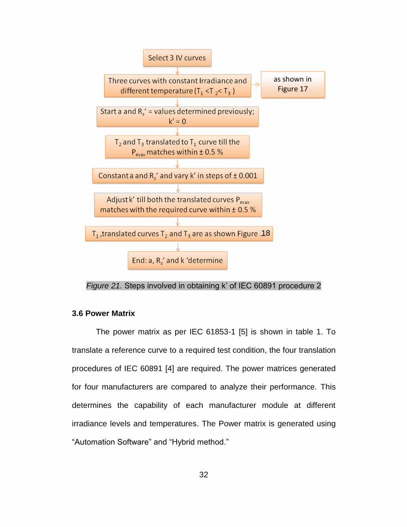
Figure 21. Steps involved in obtaining k’ of IEC 60891 procedure 2

3.6 Power Matrix

The power matrix as per IEC 61853-1 [5] is shown in table 1. To

translate a reference curve to a required test condition, the four translation

procedures of IEC 60891 [4] are required. The power matrices generated

for four manufacturers are compared to analyze their performance. This

determines the capability of each manufacturer module at different

irradiance levels and temperatures. The Power matrix is generated using

“Automation Software” and “Hybrid method.”


18

33

In the hybrid method, the power matrix uses the automation

software, but the reference cell for translation is selected by manually.

This method was used because the results produced by automation

software had deviations when compared with the real data.

34

Chapter 4

RESULTS AND DISCUSSIONS

In Previous sections, the experiment setup and methodology were

discussed. In the introduction it was mentioned that the project was

carried out on four modules from four manufacturers. For convenience,

four manufacturers are considered as four sets, each set is named as M1,

M2, and M3 and M4. In each set, the modules are numbered as M1-1,

M1-2, M1-3 and M1-4. The other 3 sets are numbered in similar pattern.

The results and discussions obtained at the various stages of the

project are presented in this section.

4.1 Automation Software

The 23 element Power Matrix according to IEC 61853-1 had to be

generated using IEC 60891 procedures. The procedures discussed in IEC

60891 have lot of math involved to obtain the required results, which

needs special expertise. The calculations involved in Procedure 1 and 2

needs extreme attention and are easily prone to human errors [8].

Procedure 3 and 4 are interpolation procedures which involve a condition

to select curves. Due to the above mentioned reasons, the first three

procedures of IEC 60891 were automated as software [1]. This software

was developed by Fernandes and was validated by the present

researcher using the data collected by Paghasian [7]. The main window of

the software is shown in Figure 22.

35

Figure 22. Automation Software Main Page

4.2 Collecting the Baseline Data

The baseline curves are collected from either three or four modules

of each set. For each set of modules, 10 baseline curves were collected

and computed using conventional baseline translation procedure as

explained in methodology chapter. The temperature coefficients were

calculated using the procedure shown in figure 23.

Apart from temperature coefficients, baseline procedure was also

used to calculate various parameters at STC conditions, as shown in

figure 23.

36

Figure 23. Conventional Baseline Procedure – An example

From each manufacturer, four similar modules were selected for

which the parameters (Temperature coefficients, Maximum Power, Fill

factor, Voc and Isc) were approximately equal. To declare four modules

similar, the IV curves at STC should lie on each other as shown in figure

24.

PV Parameters at STC conditions

Temperature Coefficients

Conventional Baseline Procedure Results of Electrical Performance and Temperature Coefficient Test

37

Figure 24. Baseline I-V Curves of four modules of Manufacturer A at STC

4.3 Mesh Calibration for Transmittance

The project demanded that the data had to be collected at various

irradiances for which meshes were used to decrease the irradiance to the

required level. Before using, the meshes were to be calibrated as

discussed in methodology chapter.

The IV curves were collected at about 1000 W/m2 irradiance

without mesh screen and at different irradiances by quickly placing

different mesh screens at a constant stabilized temperature. Once the

data collection was complete, the mesh screen was calibrated using the

relation “current is directly proportional to irradiance,” which determines

the amount of the irradiance that was transmitted. Two sets of meshes

were used in this project. Set 1 was used to collect baseline curves at

different irradiances; the calibration factors for Set 1 are presented in

Voltage (V)

Isc (A)

38

Table 2. The other set of meshes were used on top of the two axis tracker

to obtain different irradiances in the data collection.

Table 2. Mesh Transmittance Calibration of Set 1

Table 3. Mesh Transmittance Calibration of Set 2

Irradiance Transmittance

Coefficient

200 0.25

500 0.65

4.4 Data Collection on Two Axis Tracker

For data collection, each set (one manufacturer of the four) was

selected and three or four similar modules of the manufacturer were

chosen. These three or four modules were placed on the platform of a two

axis tracker. Then the output of each module was fed to the multi curve

tracer, to read the I-V Curve from the module. The module temperatures

(at the center and one of the ends of the module) were read using

thermocouples; these thermocouples were also connected to the multi-

39

curve tracer. Apart from these parameters the other parameters which

were monitored were irradiance and temperature of the reference cell.

These parameters and IV curve data were logged into a computer through

the multi-curve tracer.

Figure 25. Steps used to cleanup and obtain quality data to use as input

for the automation software

40

The data collected using the multi-curve tracer undergoes various

processing steps before it could be used for the actual power matrix

calculations as shown in Figure 25. The flow chart shows that the data

collected was in “.iva” format, but in order to do the calculations, it was

converted to excel format, i.e., “.xls” format. The next steps in organizing

the data are discussed in the figure 25. The irradiance shown by the

reference cell can be used for the calculations and when the meshes are

used the irradiances can be corrected using the mesh calibration factors.

But in this project, the irradiance was calculated by using the Isc of the

module and correcting it with the module temperature. This was done

because, the modules were left on the two axis tracker for 12 days and

there can be a non uniform dust accumulated on the modules or meshes.

The accumulated dust affects the irradiance and could be different from

the reference cell irradiance.

Once all the curves were converted, the data was fed into the

automation software. The data collected on 24th November 2011 was read

through the automation software and the graph with Temperature vs.

Irradiance data is shown in Figure 26.

The data differs from a clear sunny day to a cloudy day; the data

that is shown in Figure 26 is for a cloudy day. On a cloudy day, the data

from all the four modules appear to be mixed, and one cannot differentiate

the data from one module to the other module. But on a sunny day, the

data will be seen as clusters. The data from each module will be seen as a

41

group; therefore the graph will have four groups of data points, as there

are four modules used in this project. The data collected from the four

modules on 19th Oct 2011, which was a sunny day, is shown in Figure 27.

Therefore to avoid the clusters in the graph, the experiment should be

conducted on a cloudy day. This gives a high range of irradiances and

temperatures

Figure 26. Figure showing the raw irradiance and module temperature data obtained on 24th Nov 2011 (partially cloudy day; fall season)– with

four modules, in which two are covered with mesh screens and the other two modules with thermal insulation as explained in the experimental

setup section

Irradiance (W/m2)

Temperature (C)

42

Figure 27. Figure showing the raw irradiance and module temperature data obtained on 19th Oct’11 (clear sunny day; fall season) – with four

modules, in which two are covered with mesh screens and the other two modules with thermal insulation as explained in the experimental setup

section

In Figure 26 and Figure 27, the graph is plotted to show the data

points as “Temperature vs. Irradiance.” Figure 28 (below) shows the graph

of automation software which plots the data points as “Current vs.

Voltage.”

25 % T Mesh, No Insulation

65 % T Mesh, With Insulation

No Mesh, No Insulation

No Mesh, With Insulation

Temperature (C)

Irradiance (W/m2)

43

Figure 28. Data collected on 19th Oct.11 from Module 3

On a cloudy day, when there is a cloud passing at the time of I-V

Curve measurement, those I-V curves would have a small drop or a

shoulder in the middle of the curve. Sometimes the curve would have

more than one shoulder, as shown in Figure 29. The data in the Figure 26

shows the data points on a cloudy day, so the curve shown in Figure 29 is

from the set of data points of Figure 26. One I-V curve will be taken within

7 seconds, but still the module is affected by the passing cloud. If there is

no cloud when the data is collected, then we get a curve, as shown in

Figure 30. So from this it is clear that, when there is a passing cloud, a

Voltage (V)

Current (A)

44

dip will be seen in the curve. This is similar to having a non- uniform

shadow on the module.

Figure 29. I-V Curve when there is a passing cloud

When the curves were observed closely, it was found that there are

many curves with dips due to passing clouds. This is because the data

was collected in the fall season. There is an advantage and disadvantage

of collecting the curves in the fall. The advantage is that we can have a

slow increase in the temperature in a day and have curves at various

temperatures and irradiances. The data points spreads throughout the

graph. But when it is taken on a clear sunny day, the data points will be as

clusters rather than being spread throughout the graph. This was shown in

Figure 29 and Figure 30.

Voltage (V)

Current (A)

45

Figure 30. IV Curve taken when there is no passing cloud

It was observed that there are many curves with dips in the data

collected from a single day, as shown in Figure 31. Due to the irregularity

in the data which was collected on cloudy days, the linearity check was

performed to remove the affected curves and have high quality data. By

deleting the outliers in the data, the results produced with the new set of

curves give better results.

Voltage (V)

Current (A)

46

Figure 31. Single day Data set from Module 1 of M2, showing curves on a cloudy day

To perform the linearity check, various graphs are plotted – Isc vs

Irradiance and (Isc/ Irradiance) vs Irradiance. These graphs help in

removing the outlier data. Figure 32 shows Isc Vs Irradiance plot and

Figure 33 shows the (Isc/Irradiance) vs Irradiance plot with irregular data.

From Figure 32, a line can be seen, which seems to pass through origin,

so any data point that was out of that imaginary line was deleted. In Figure

33, the data points seem to be constant at any irradiance point. The data

point that was within the 3% limits is used for the calculations and all other

data points that are outside the limits were deleted in this graph. Figure 34

Voltage (V)

Current (A)

47

shows the figure 32 data after deleting the outlier data and similarly figure

35 shows the figure 33 data after getting rid of outlier data.

Figure 32. Isc Vs Irradiance data without clearing the irregular data

Figure 33. Isc/Irradiance Vs Irradiance data without clearing the irregular data

Irradiance (W/m2)

I sc (

A)

Isc vs Irrd

Isc/Irrd vs Irrd

Irradiance (W/m2)

I sc/I

rra

d (

Ratio

)

48

Figure 34. Isc Vs Irradiance data after cleaning up the irregular data that was shown in Figure 24

Figure 35. Isc/Irradiance Vs Irradiance data after removing the outlier data in Figure 25

Irradiance (W/m2)

I sc (

A)

Isc - Irrd

I sc/I

rra

d (

Ratio

)

Isc/Irrd - Irrd

Irradiance (W/m2)

49

4.5 Parameters

After the data was cleaned up using the linearity check, the data

was used for further calculations.

Each procedure has a set of parameters which need to be

calculated, before the data is used to generate the Power Matrix.

Temperature coefficients are calculated before any calculations are

performed and this was already discussed in baseline procedure. Once

the temperature coefficients are obtained the other parameters such as

(Rs, k) for procedure1 and (a, Rs’, k’) for procedure 2 were calculated. As

all the parameters were obtained the power matrices were generated

using first three procedures of IEC 60891 [4]. The Power matrices for the

four manufacturers were calculated and compared. . The comparison is

done in terms of percentage for all the 23 elements in the power matrix.

Consider a hypothetical module of 100 W power which has

constant efficiency at all irradiance levels and temperature coefficient of

power as -.5%/C. The power matrix of this module is shown in Table 4.

50

Table 4. Power Matrix for hypothetical 100 W module

Irradiance (W/m2) Temperature (oC)

15 25 50 75

1100 N/A 110 96.25 82.5

1000 105 100 87.5 75

800 84 80 70 60

600 63 60 52.5 45

400 42 40 35 N/A

200 21 20 17.5 N/A

100 10.5 10 N/A N/A

Note: Power temperature coefficient is - 0.5 %

The power matrix that is shown in the Table 4 is an ideal

representation, where the power temperature coefficient of a particular

module is -0.5%/oC at all irradiance levels. But in reality, the modules of

different manufacturers may have different temperature coefficients and

these coefficients may depend on the irradiance levels. It is not only true

for power temperature coefficients, but also for the temperature

coefficients of voltage and current. In this study, four similar modules are

considered from each manufacturer. When the temperature coefficients

were calculated using baseline procedure, the temperature coefficients for

all the four modules were not same but approximately equal. The

difference in temperature coefficients for four modules of same

manufacturer/ different manufacturers was due to the presence of

parasitic resistances. The parasitic resistances and its effects are already

discussed in the methodology chapter.

51

4.6 Validation of Automation Software

Automation software was developed for the translation procedures

of IEC 60891 and power matrix generation of IEC 61853-1 using the first

three procedures [1]. Before the automation software was used for this

project, it was validated. The data used for the validation was collected on

the Mono Crystalline Module [7] (Paghasian, 2010). The data was used to

generate the power matrix of IEC 61853-1 using procedure 2 of IEC

60891. The power matrix was generated using both manual process using

Microsoft Excel and the automation software. The percentage (%)

difference between the results of manual and automation is shown in

Table 5.

Table 5. Comparison of Manual and Automation results of mono crystalline module [7] (Paghasian, 2010)

Irradiance

15 25 50 75

1100 N/A -0.4% -0.3% -0.3%

1000 0.2% 0.2% 0.3% -0.4%

800 -0.1% 0.1% -0.1% -0.1%

600 -0.5% -0.5% -0.6% -0.7%

400 0.4% 0.4% 0.4% N/A

200 1.8% 1.8% 1.7% N/A

100 -0.1% 0.7% N/A N/A

4.7 Validation of First Two Procedures of IEC 60891

For each manufacturer, the data was collected as discussed in the

Introduction and Methodology chapters. The setup for the data collection

52

is shown in Figure 9. The data was collected every 2 minutes from the four

modules for 12 continuous days. The power matrix was calculated for four

modules at 1 day, 6 days, and 12 days. The power matrix for a particular

module was calculated according to the first two procedures of IEC 60891.

The percentage (%) difference between the two power values of

procedure 1 and 2 of IEC 60891 was calculated for all 23 elements of a

power matrix and is presented in Table 6. Whenever the percentage (%)

difference was less than 3%, it was considered to be acceptable. In table

6, all the percentages are less than 3%. Therefore, to generate the 23

elements of a power matrix for any module, one can use any of the two

procedures.

Table 6. Comparison between Procedure 1 and Procedure 2 for M2 considering four modules for 12 days

Comparison of procedure 1 & 2

Irradiance (W/m2)

Temperature (oC)

15 25 50 75

1100 N/A -1% 0% -1%

1000 0% 0% 0% 0%

800 1% 0% 0% 0%

600 1% 2% 1% 0%

400 1% 1% 0% N/A

200 0% 0% 0% N/A

100 0% -1% N/A N/A

53

4.8 Comparison of Power Matrices of a Manufacturer at Different

Conditions

The power matrices are calculated for each manufacturer at different

conditions. The conditions are:

4 modules and 12 days

4 modules and 6 days

4 modules and 1 day

1 module and 12 days

1 module and 6 days

1 module and 1 day

Once the power matrix was calculated for each of the above

conditions, they were compared to identify the differences between the

power matrices for each manufacturer.

4.8.1 One manufacturer, four modules.

A single manufacturer (M3) is considered in this section. The data

from four modules of Manufacturer 3 were used for the calculations and

the power matrices were generated using procedure 1. In table 7, the

power matrices are compared, which gives information on percentage (%)

difference between the 23 elements of a power matrix generated for 1 day

and 6 days. Table 8 gives the comparison between1 day and 12 days and

table 9 gives the comparison between 6 days to 12 days.

54

Table 7. Comparison of a power matrices generated for 4 modules of Manufacturer 3 using procedure 1 between 1 day and 6 days

Irradiance (W/m2)

Temperature (oC)

15 25 50 75

1100 N/A -2% 0% 0%

1000 2% -2% 0% 0%

800 4% 2% 0% 0%

600 -3% -2% 1% 0%

400 -3% 0% 4% N/A

200 0% 3% 3% N/A

100 2% -7% N/A N/A

Table 8. Comparison of a power matrices generated for 4 modules of Manufacturer 3 using procedure 1 between 1 day and 12 days


15 25 50 75

1100 N/A -3% 0% 0%

1000 0% -4% 0% 0%

800 1% 1% 0% 0%

600 -3% -2% 1% 0%

400 0% 0% 7% N/A

200 0% 3% 6% N/A

100 1% -6% N/A N/A

55

Table 9. Comparison of a power matrices generated for 4 modules of Manufacturer 3 using procedure 1 between 6 days and 12 days

From the results in Tables 7, 8, and 9 the following can be concluded –

(i) The percentage (%) differences in the power matrices are

higher when compared between 1 day and 12 days as shown in

figure 8.

(ii) The percentage (%) differences in the power matrices were

lower than the table 8 when it is compared between 1 day to 6 days

as shown in table 7, i.e., the number of points nearer to 0% is more

when compared with table 8.

(iii) The percentage (%) differences in the power matrices when

compared for 6 days to 12 days as shown in table 9 are within 3%

and maximum points have the deviation to be zero.

(iv) This concludes that, as the number of days of data collection

increases the results would be more accurate and nearer to actual

value.

Irradiance (W/m2) Temperature (C)

15 25 50 75

1100 N/A 0% 0% 0%

1000 -2% -2% 0% 0%

800 -3% -1% 0% 0%

600 0% 0% 1% 0%

400 3% 0% 3% N/A

200 0% 0% 3% N/A

100 -1% 0% N/A N/A

56

The power matrices generated at 1 day, 6 days, and 12 days for

the 4 modules of same manufacturer M3 were considered for the next

study. For the next study, these power matrices are compared with the

idle power matrix, where the power temperature coefficient is -0.5% and

efficiency is constant throughout the matrix. In this, each element of the

power matrix was compared with the idle power at that point. The idle

power at different irradiance levels was directly proportional to the

irradiance.

The comparison between the calculated power and idle power is

shown in terms of percentage (%) deviation. The tables 10, 11 and 12

show the percentage deviations for 1 day, 6 days and 12 days

respectively of four modules of M 3 Manufacturer.

Table 10. Comparison of idle and calculated power for 1 day data of four modules for M3

1 day

Procedure 2 - Power Matrix (W)

Irradiance (W/m2) Temperature (C)

15 25 50 75

1100 N/A 0% -2% -1%

1000 0% 0% 0% 0%

800 0% 1% 1% 2%

600 1% 2% 4% 2%

400 1% 1% 3% N/A

200 0% 0% 0% N/A

100 -1% -1% N/A N/A

57

Table 11. Comparison of idle and calculated power for 6 days data of four modules for M3

6 days



Desired G (W/m2) 15 25 50 75

1100 N/A 0% -2% -1%

1000 0% 0% 0% 0%

800 0% 1% 1% 2%

600 1% 2% 4% 1%

400 1% 0% 1% N/A

200 0% -1% 0% N/A

100 0% -1% N/A N/A

Table 12. Comparison of idle and calculated power for 12 days data of four modules for M3

12 days


Irradiance (W/m2)

Temperature (oC)

15 25 50 75

1100 N/A -1% -1% -1%

1000 0% 0% 0% 0%

800 1% -1% 1% 3%

600 1% 0% 2% 1%

400 0% -1% 1% N/A

200 0% -1% 0% N/A

100 -1% -1% N/A N/A

58

Tables 10, 11, and 12 clearly demonstrate which of the sets of data

gives the best results. The deviations of the power matrices for the three

sets of data are compared. From the deviations, it is understood that as

the number of days increase, the deviation decreases. The percentage

deviations are least for 12 days data.

From the above two discussions, it is clear that 12 days data

produces the power that is nearer to the estimated power. The next best

data is obtained from 6 days data.

4.8.2 One manufacturer, one module (no mesh, no insulation).

The study discussed in the previous section was done on four

modules of a manufacturer M3. In this section, the deviations were

calculated in a similar manner as done in the previous section for single

manufacturer, single module. In this section, one module (M3-3) of

manufacturer M3 was considered. The module that was selected was

without mesh and insulation on the back. This particular module was

considered, as it did not have a mesh which reduces the irradiance on the

module or an insulation to increase the module temperature. In this

section it compares the percentage (%) deviation between the 23

elements of power matrix of calculated power for a single module to the

idle power.

For this module, the power matrices were calculated for 1 day, 6

days, and 12 days. After the power matrices were generated the

percentage (%) deviations were calculated between the idle power and

59

calculated power for all the 23 elements of the power matrix. The

percentage (%) deviations were calculated and projected in the Table 13

is for 1 day data, Table 14 for 6 days data and Table 15 for 12 days data.

Table 13. Comparison of idle and calculated power for 1 day data of one module of M3

1 day


Irradiance (W/m2)

Temperature (oC)

Desired G (W/m2)

15 25 50 75

1100 N/A 0% -2% 0%

1000 0% 0% 0% 0%

800 0% 3% 1% 2%

600 -5% -2% 4% 5%

400 0% 1% -2% N/A

200 -2% -1% -2% N/A

100 -2% -3% N/A N/A

Table 14. Comparison of idle and calculated power for 6 days data of one module of M3

6 days


Irradiance (W/m2)

Temperature (oC)

Desired G (W/m2)

15 25 50 75

1100 N/A 0% -2% 0%

1000 0% 0% 0% 0%

800 -1% -1% 1% 2%

600 1% -6% 4% 5%

400 1% 0% 0% N/A

200 -1% -1% -1% N/A

100 -2% -1% N/A N/A

60

Table 15. Comparison of idle and calculated power for 12 days data of one module of M3

12 days


Irradiance (W/m2)

Temperature (oC)

Desired G (W/m2)

15 25 50 75

1100 N/A -1% -2% 0%

1000 0% 0% 0% 0%

800 -1% -1% 1% -1%

600 0% 0% 4% 2%

400 -2% -1% 0% N/A

200 -2% -1% -1% N/A

100 -2% -2% N/A N/A

From tables 13, 14 and 15; we get the same information as in the

previous section. It is once again proved that as the number of days

increase, the percentage (%) deviation decreases. Therefore, the table 15

has least percentage (%) deviations compared to table 13 and 14.

4.8.3 Comparison of 12 days data of one module (no mesh, no

insulation) to four modules of same manufacturer. It is concluded that

the deviation is least when the power matrix is generated for 12 days data

either with one module or four modules. In this section, the power matrices

of one module and four modules are compared for 12 days of

manufacturer M3. This comparison is shown in table 16, which gives

information about the percentage (%) deviation of one module to four

modules.

61

Table 16. Comparison of Power between 4 modules data to 1 module data for 12 days of M3 manufacturer



15 25 50 75

1100 N/A 0% 0% 2%

1000 -2% 0% 0% 3%

800 0% 0% 0% 4%

600 0% 0% -2% -3%

400 1% -1% 3% N/A

200 8% 0% 5% N/A

100 9% 14% N/A N/A

Though the power matrix in table 15 shows that the percentage (%)

deviation is low, but it is high when compared to table 12. This is because,

in table 15, the power deviations are calculated in comparison with the idle

power but not the actual power. The percentage (%) deviations are

calculated for table 12 to table 15 is shown in table 16. The percentage

(%) deviations are more than ± 3 %.

4.9 Power Matrix Generated Using Procedure 3

In the whole discussion, we considered only the first two

procedures of IEC 60891 as the other two procedures of IEC 60891 were

not able to generate the power for all the 23 elements of the power matrix.

This was because the translation was done only by using interpolation

method, but for interpolation the curves need to be outside the required

curve as it was shown in methodology chapter. When the data is collected

62

for this procedure, there was no chance to collect the data at required

condition. Therefore in procedure 3, the powers were calculated only at

few points, where the curves were available for interpolation as shown in

figure 36.

Figure 36. Power Matrix generated with procedure for four modules of M1using 12 days

The graph has various colors to differentiate the power at different

temperatures. The color coding is done for each temperature.

4.10 Comparison of Efficiencies of a Manufacturer at Different

Conditions

For a particular module, after calculating the Power Matrices at

different conditions, the efficiency is calculated by taking its area into

account. In Figure 37, we can see the efficiency of one particular

manufacturer by considering the data of four modules for 12 days. Figure

63

37 gives information of a manufacturer at four different temperatures (15

C, 25 C, 50 C and 75 C).

Figure 37. Efficiency of a manufacturer (4 modules and 12 days) at four different temperatures

The other three manufacturers also give a similar Efficiency (%) vs.

Irradiance (W/m2) graph. The data points considered in the Figure 37 are

from the power matrix.

In the figure 37, it is seen that the efficiency of the module drops as

the temperature of the module increases. Apart from that, it is also

observed that as the irradiance decreases from 1100 W/m2 towards 600

W/m2 the efficiency increases. But after 600 W/m2 the efficiency

decreases as the irradiance decreases. The initial increase in the

efficiency was due to the series resistance and later decrease in efficiency

was due to the shunt resistance. The graph in figure 37 is a good example

64

for the influence of the parasitic resistance on the efficiency of PV

modules. It shows how the series resistance and shunt resistance affect

the efficiency of the module (actually the power of the module).

Considering the 15C plot in the figure 37, the efficiency decreases even

though the irradiance increases from 600 W/m2 to 1000 W/m2 because of

the series resistance affect. But from 400 W/m2 to 100 W/m2, the

irradiance decreases and efficiency also decreases. In this case the

efficiency is affected by the shunt resistance. The drop is even high when

compared to irradiance, as the shunt resistance is very high. Now for a

single manufacturer, four modules of data are considered for 1 day, 6

days and 12 days. The efficiencies are calculated for all the 23 elements

of the power matrix for the three sets of data. Figure 38 gives the

efficiencies for 1 day data at seven different irradiance levels and four

different temperatures. The next two figures, Figure 39 and Figure 40, give

similar information but for 6 days and 12 days respectively of the same

manufacturer. These three power matrices are generated using the

automation software.

65

Figure 38. Efficiency of a manufacturer (4 modules and 1 day) at four different temperatures


66


In figure 38, the efficiency dropped at 600 W/m2 in 15 C and 25 C

plot. But in figure 39 the efficiency increased at 15 C; still there is a drop

seen at 25 C. When it is seen in Figure 40, the efficiency plot is similar to

the plot shown in figure 37.

From the above three figures, it is again proved that the power

matrix generated for 12 days gives better results compared to the 1 day

and 6 days data. In figure 38 and figure 39, a sudden drop in the graph is

observed. But later in the efficiency graph figure 40 which has 12 days

data, looks better. This is because when there are less data points, there

is chance of not having exact or closest curve to translate it to the required

67

data point. When the translation is done from a far data point, then the

deviation is high; this is what is seen as a drop in figure 38 and figure 39.

4.11 Comparison of Four Manufacturers

The four manufacturer efficiencies are compared at different

temperatures. These graphs best explain the differences in the efficiencies

for four manufacturers at different irradiance levels and constant

temperature. Figure 41 compares the efficiencies of four manufacturers at

seven different irradiances, but at 15C. Similar graphs are shown in

Figure 42 at 25C, Figure 43 at 50C and Figure 44 at 75C temperatures.

Figure 41. Comparison of Efficiencies at different Irradiance levels and at

constant temperature of 15 C

68





69



The main purpose of the comparison is to identify the best module

which suits the region where the installation needs to be done. The three

main required criterions are:

Price of the Module

Efficiency of the module

Area required to meet the required power

The comparison is done in respect of the price of the modules. In

figure 43 at 600 W/m2 and 50 C, the M2 and M3 have same efficiencies.

Therefore the installer can choose one of them depending upon the price

of the module.

The next comparison for manufacturers is for the efficiencies of the

modules. The installer wants to install the modules with higher efficiency

70

to reduce required roof/land area along with reduction of structural cost.

With the old method of module rating, the efficiencies of the PV modules

were labeled only at STC conditions. But in reality the modules need to be

installed at different environmental conditions from that of the labeled

conditions. In this case the power matrix helps the installer to select the

module which has more efficiency at the required environmental

conditions. In figure 42 at STC conditions the M2 manufacturer has higher

efficiency compared to M4. But if the modules need to be installed at 400

W/m2 and 25C then M4 manufacturer is more suitable as it has higher

efficiency than M2. This is the main advantage for the installer when a

power matrix is used.

The next criterion for the installer is the area of the installation. To

explain this, let’s consider two hypothetical modules, each with 100 W/m2

but with different areas. The one with the less area and same power

occupies less space in installation. For this the module with more

efficiency will occupy less area in installation. Therefore, to occupy less

area the installer need to select a module with high efficiency.

The above discussion clearly explains that the installer needs to

pay attention on how much power the module produces at the required

test conditions. The installer can get the required power if the modules are

rated according to the IEC 61853-1 (Power Matrix at seven irradiances

and four temperatures).

71

Usually, when comparing two or more manufacturer modules,

irradiance of that region is taken as a reference. This is because the

irradiance effect is more when compared to the temperature of the region.

The next graph shown in figure 45 compares the efficiencies of four

manufacturers at different temperatures, but at a constant irradiance

(1000 W/m2).

Let’s consider an installation of solar modules on a roof top at

Mesa, AZ. In this region, majority part of the year the irradiance is

expected to be around 1000 W/m2. But the modules will experience more

than 50C temperatures. Therefore, figure 45 indicates that at STC

conditions M2 is having higher efficiency compared to M3, but the same

graph indicates that at 50C temperatures, M3 is having higher efficiency

compared to M2. This is a good example for the installer in regard to

selecting a particular model for the region.

72

Figure 45. Comparison of Efficiencies at constant Irradiance @ 1000

W/m2 and different temperature

4.12 Advantages and Disadvantages of Automation Software

There are various options built in to automation software. The

options embedded in the automation software are:

4.12.1 Single-step automation. The data analyzer has to feed the data

collected; by clicking this button, the software calculates all the

parameters. The program starts its calculations with the baseline

parameters and then calculates the individual parameters for each

procedure. Once the required parameters are calculated, the power

matrices will be calculated with provided data.

73

4.12.2 Multiple-step automation. The data analyzer has to feed the

collected data into the automation software. Once the data is fed into the

software, data analyzer next steps are:

(i) Calculate the baseline parameters

(ii) Calculate the parameters for each procedure

(iii) By clicking the multiple steps button—for example, “Multiple

Steps Automation – Procedure 1”—the software uses the

parameters calculated by the analyzer and produces the

Power Matrix by selecting the nearest and appropriate curve.

Initially the project was started with this method for research and

calculated the power matrices for all the manufacturers using Procedure 1

and Procedure 2. It was also planned to perform the analysis using

Procedure 3 but, due to limitations, this procedure was not considered.

The limitations will be discussed later in this chapter.

4.12.3 Hybrid method (manual + automation). The previous method

had some disadvantages, therefore this method was introduced. There

were limitations to the previous method. As the number of curves was

more than five thousand, the system picks up the best curve for

translation. But for the translations, the best curve has a different definition

than what the software was designed for. The irradiance of the curve

should closely match with the required condition but the temperature

difference can be high. At the same time, if the irradiance is different, very

74

little and the temperature difference is very high then the temperature

parameter should be given more importance.

As the priorities are changing according to the required curve

conditions, the curves need to be selected. The present software need to

be modified to perform the calculations as discussed in this section. But in

the available software, the analyzer can only set a ratio between the

irradiance and temperature but cannot make the software to select a right

curve when there is more than one curve available for translation.

As this issue sprang up in the project, the curves were to be

selected manually by checking which curve fits the best for the translation.

The selection is done by selecting the curve that is nearest to the required

conditions and then translation is applied to that particular curve to the

required condition by using either Procedure 1 or 2.

The comparison of the power matrices obtained from multiple step

automation and hybrid method is shown in Table 17. In both the methods,

the power matrix is obtained using procedure 2.

75

Table 17. Comparison of multiple steps automation to hybrid method for M3 using procedure 2

Comparison of Automation method to Hybrid method

Irradiance (W/m2)

Temperature (C)

15 25 50 75

1100 N/A 0.1% 2.5% -1.7%

1000 4.1% 0.5% 2.0% -2.8%

800 3.8% 2.3% 2.0% -4.4%

600 3.7% 1.6% -1.5% -0.8%

400 3.5% 1.2% -1.2% N/A

200 -0.2% 0.2% -4.7% N/A

100 -0.9% 0.4% N/A N/A

In Table 17, it is observed that 25% of the points in matrix have

percentage deviations between two methods, either less than – 3% or

more than + 3%. The other 50% have the percentage deviation either less

than – 1% or more than + 1%. Therefore only 25% of the points in the

matrix have the deviation percentage between ± 1%. This concludes that

the deviation is high between two methods and it was observed that the

power matrix generated using multiple steps automation is not meeting the

conditions when cross checked with parameters such as maximum power

at STC, temperature coefficients, etc.

The powers generated by the automation software and hybrid

method at STC are compared with the module rated power. This

comparison is shown in table 18. This table clearly explains that the hybrid

method produces best results compared to the automation software.

76

Table 18. Comparison of module rated power at STC with the powers calculated using automation software and hybrid method

Rated Power Power generated using Automation Software

Power generated using Hybrid Method

0% -5.1% 0.1%

4.13 Comparison between Four Procedures of IEC 60891

The IEC 60891 has two procedures (Procedure1 and Procedure 2)

which are based on the translation phenomenon. The other two

procedures (Procedure 3 and Procedure 4) are based on interpolation

phenomenon. The four procedure are discussed in the methodology

chapter, where it is explained how each procedure works.

These four procedures of IEC 60891 have their own advantages

and disadvantages and these are compared in table 19.

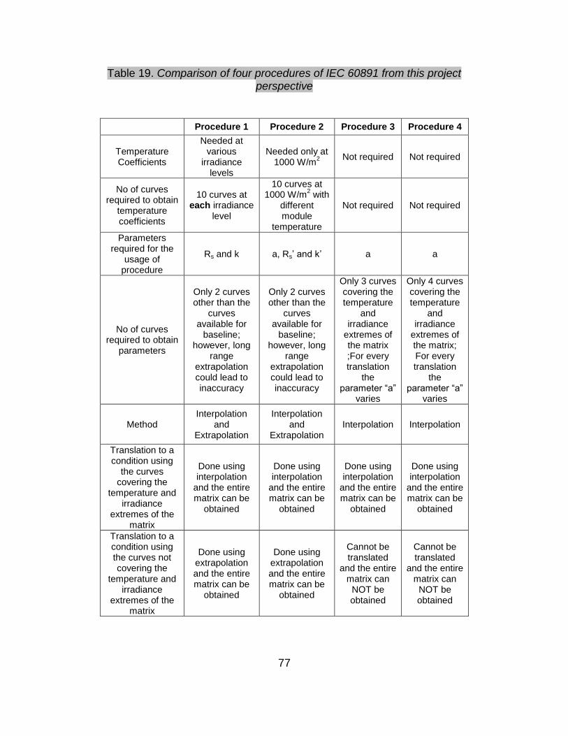
77

Table 19. Comparison of four procedures of IEC 60891 from this project perspective

Procedure 1 Procedure 2 Procedure 3 Procedure 4

Temperature Coefficients

Needed at various

irradiance levels

Needed only at 1000 W/m

2

Not required Not required

No of curves required to obtain

temperature coefficients

10 curves at each irradiance

level

10 curves at 1000 W/m

2 with

different module

temperature

Not required Not required

Parameters required for the

usage of procedure

Rs and k a, Rs’ and k’ a a

No of curves required to obtain

parameters

Only 2 curves other than the

curves available for

baseline; however, long

range extrapolation could lead to inaccuracy

Only 2 curves other than the

curves available for

baseline; however, long

range extrapolation could lead to inaccuracy

Only 3 curves covering the temperature

and irradiance

extremes of the matrix ;For every translation

the parameter “a”

varies

Only 4 curves covering the temperature

and irradiance

extremes of the matrix; For every translation

the parameter “a”

varies

Method Interpolation

and Extrapolation

Interpolation and

Extrapolation Interpolation Interpolation

Translation to a condition using

the curves covering the

temperature and irradiance

extremes of the matrix

Done using interpolation

and the entire matrix can be

obtained



obtained



obtained



obtained

Translation to a condition using the curves not covering the

temperature and irradiance

extremes of the matrix

Done using extrapolation and the entire matrix can be

obtained

Done using extrapolation and the entire matrix can be

obtained

Cannot be translated

and the entire matrix can

NOT be obtained

Cannot be translated

and the entire matrix can

NOT be obtained

78

Procedure 1 and 2 can translate any curve to any required

condition using the temperature coefficients and the parameters required

for that particular procedure. Procedure 2 requires only 12 curves on total

to obtain the curve at any condition. But as the number of curves increase

the deviation percentage of Pmax decreases.

But Procedures 3 and 4 have many limitations. These procedures

can generate any condition in the power matrix, even if it has 4 curves

covering extreme temperatures and irradiances of the matrix. However,

long-range interpolation may lead to inaccurate results due to the

influence of irradiance on fill factor. When having 4 curves, the below

mentioned conditions are to be met –

Irradiance less than 100 W/m2 and at least one curve at

temperature less than 15 C and one curve at temperature more

than 75oC.

Irradiance more than 1100 W/m2 and at least one curve at

temperature less than 15 C and one curve at temperature more

than 75oC.

But to have these conditions, it was practically difficult with the test

setup used in this study. It is possible to have such curves only by using

an external heating or cooling system behind the module. Irradiance

nearer to 1100 W/m2 can frequently be obtained in summer; so to have

these irradiances; the tests need to be conducted primarily in summer

season. At the same time, these four curves are not enough to have

79

accurate results. Paghasian [7] proved that to have less percentage

deviation between the translated curve and actual curve, the reference

curve needs to be nearer to the required condition.

As the project’s main aim was to use the natural sunlight and

natural heating or cooling process, the above discussed procedure is not

applicable for this project

.

4.14 Power Temperature Coefficient

The module data sheet indicates the power temperature coefficient of the

module at the STC conditions only. As the efficiency and power varies

with the irradiance so does the power temperature coefficient. The change

in the power temperature coefficient is shown in figure 46.

Figure 46 – Comparison of the power temperature coefficients at various irradiance levels for M1 manufacturer

80

From the figure explains that, the power temperature coefficient is

directly proportional to the irradiance. As the irradiance decreases, the

power temperature coefficient decreases.

81

Chapter 5

CONCLUSIONS AND RECOMMENDATIONS

5.1 Conclusions

5.1.1 Number of Days Required for Data Collection –

The power matrices generated using monitored data for one, six

and twelve days were compared. It is concluded that the power matrix

generated based on twelve days was the best, though the improvement

was found to be very minimal when compared with the matrix generated

based on six days.

5.1.2 Procedure selection –

Based on the test setup used in this work, the procedure 2 of IEC

60891 was selected for all data processing. This is because the procedure

1 required more number of performance parameters to be calculated as

compared to procedure 2. Even though procedure 3 and procedure 4 do

not require more than one parameter, they require monitored data at or

above temperature and irradiance levels specified in the IEC 61853-1

standard. The experimental setup used in this work could not collect data

at these extreme temperature and irradiance levels, and hence the matrix

generation based on procedure 3 or procedure 4 is not included in this

work.

82

5.1.3 Software Validation –

In this report the power matrices were generated using both the

automation software developed in a previous work and the hybrid method

utilized in this work.

It is demonstrated that the maximum power determined at STC

conditions using the hybrid method was closer to the actual measured

power using the conventional baseline method established at ASU-PRL. It

was observed that the percentage deviation for automation software was

as high as -5.1% and for hybrid method it was only +0.1% when compared

with the actual baseline power at STC. This demonstrates that the hybrid

method provides more accurate results than the automation software. The

automation software needs some improvement as described in the

recommendation section below.

5.1.4 New Outdoor Test Method –

For power matrix calculation, Sandia National Laboratories method

requires collection of I-V curves continuously throughout a day or two from

a single module mounted on a two axis tracker. Since the Sandia test

setup does not use thermal insulators on the back side of the test module

to obtain data at high temperatures or mesh screens in front of the test

module to obtain data at low irradiances, the availability of sufficient

number of data for regression analysis at low irradiances and high

temperatures could be challenging depending on the season. In this

83

research a new outdoor test setup was used, in which four similar or

practically identical modules were placed on a two axis tracker to collect

the data throughout the day. These four modules were set to collect data

at different irradiances and temperatures. To have data at low irradiance

levels, two of the modules were covered with mesh screens. At the same

time two other modules were back insulated to have higher temperatures.

The data collected using this new test setup covered a wide range of

irradiance and temperatures required to generate the matrix of IEC 61853-

1 standard.

5.1.5 Comparison of power temperature coefficient at various

irradiance levels –

Whenever the module maximum power is to be calculated at different

temperatures other than 25oC, the power temperature coefficient obtained

at a single irradiance of 1000 W/m2 is used for the calculations. In this

study it was observed that the power temperature coefficient of the

module is not constant. It has a dependence on the irradiance level and

hence the use of single power temperature coefficient for all irradiance

levels is discouraged.

84

5.1.6 Comparison of Different Manufacturers –

One of the primary aims of the project was to find out the best suited

module for particular field conditions using Efficiency vs. Temperature and

Efficiency vs. Irradiance plots.

This study concludes that the efficiency of the PV modules is not

constant at all irradiance levels and it could dramatically decrease at very

low irradiance levels depending on the quality of the cells used in the

module. . These variations from one cell/module manufacturer to another

cell/module manufacturer have been clearly seen in this study and they

are attributed to the cell parameters such as varying power temperature

coefficient, series resistance and shunt resistance. Based on the test

method developed in this study, a suitable module for a specific site

condition could be selected by screening a large number of modules with

minimal number of labor hours.

5.2 Recommendation

In this study, procedure 3 and procedure 4 were unusable due to

natural limitations on temperature controllability. Further research

may be conducted with more controllability on temperature. With

this improvement, all the four procedures of IEC 60891 and NREL

can be used to analyze the data.

85

The automation software should be improved to select a reference

curve closest to the target condition; this selection was done

manually (Hybrid Method which utilized the manual selection of

reference curves and the automatic data processing) in this

research.

The current version of automation software generates only Pmax

matrix; however, the IEC 61853-1 standard requires generation of

other matrices including Isc and Voc. Therefore, the automation

software should be further improved to generate all the matrices

required by the IEC 61853-1 standard.

86

REFERENCES

[1] Fernandes, M. (2011). Automation of Current-Voltage Translation Procedures of Photovoltaic Modules per IEC 60891 and IEC 61853-1 Standards. (Master’s Thesis). Arizona State University, AZ. [2] Honsberg, C. and Bowden, S. (2010). Resistive Effects. PVCDROM. Retrieved from: http://pvcdrom.pveducation.org/ [3] International Electrotechnical Commission (2009a). IEC 60904-10: Photovoltaic devices – Methods of linearity measurement, 2nd ed. [4] International Electrotechnical Commission (2009b). IEC 60891: Photovoltaic devices – Procedures for temperature and irradiance corrections to measured I-V characteristics, 2nd ed. [5] International Electrotechnical Commission (2010). IEC 61853-1 (Draft): Photovoltaic (PV) Module Performance Testing and Energy Rating. [6] Lad, R (2010). Outdoor Performance Rating and Spectral Effects of Photovoltaic Modules. (Master’s Thesis). Arizona State University, AZ. [7] Paghasian, K (2010). Power Rating of Photovoltaic Modules: Repeatability of Measurements and Validation of Translation Procedures. (Master’s Thesis). Arizona State University, AZ. [8] Tamizhmani, G., Paghasian, K., Kuitche, J., et al. (2011). Photovoltaic Module Power Rating per IEC 61853-1 Standard. Solar America Board of Codes and Standards ABCS-18-SR. Retrieved from http://www.solarabcs.org

http://pvcdrom.pveducation.org/

http://www.solarabcs.org/

power rating of photovoltaic modules using a new outdoor ... · i would like to thank dr. narcio f....

Documents