power generation technology data for integrated resource plan of south africa
TRANSCRIPT

Power Generation Technology Data for Integrated Resource Plan of South Africa


EPRI Project Manager G. Ramachandran
ELECTRIC POWER RESEARCH INSTITUTE 3420 Hillview Avenue, Palo Alto, California 94304-1338 ▪ PO Box 10412, Palo Alto, California 94303-0813 ▪ USA
800.313.3774 ▪ 650.855.2121 ▪ [email protected] ▪ www.epri.com
Power Generation Technology Data for Integrated Resource Plan of South Africa
EPRI Member Specific Final Report, July 2010
Project Manager M. Barry
System Operations and Planning

DISCLAIMER OF WARRANTIES AND LIMITATION OF LIABILITIES
THIS DOCUMENT WAS PREPARED BY THE ORGANIZATION(S) NAMED BELOW AS AN ACCOUNT OF WORK SPONSORED OR COSPONSORED BY THE ELECTRIC POWER RESEARCH INSTITUTE, INC. (EPRI). NEITHER EPRI, ANY MEMBER OF EPRI, ANY COSPONSOR, THE ORGANIZATION(S) BELOW, NOR ANY PERSON ACTING ON BEHALF OF ANY OF THEM:
(A) MAKES ANY WARRANTY OR REPRESENTATION WHATSOEVER, EXPRESS OR IMPLIED, (I) WITH RESPECT TO THE USE OF ANY INFORMATION, APPARATUS, METHOD, PROCESS, OR SIMILAR ITEM DISCLOSED IN THIS DOCUMENT, INCLUDING MERCHANTABILITY AND FITNESS FOR A PARTICULAR PURPOSE, OR (II) THAT SUCH USE DOES NOT INFRINGE ON OR INTERFERE WITH PRIVATELY OWNED RIGHTS, INCLUDING ANY PARTY'S INTELLECTUAL PROPERTY, OR (III) THAT THIS DOCUMENT IS SUITABLE TO ANY PARTICULAR USER'S CIRCUMSTANCE; OR
(B) ASSUMES RESPONSIBILITY FOR ANY DAMAGES OR OTHER LIABILITY WHATSOEVER (INCLUDING ANY CONSEQUENTIAL DAMAGES, EVEN IF EPRI OR ANY EPRI REPRESENTATIVE HAS BEEN ADVISED OF THE POSSIBILITY OF SUCH DAMAGES) RESULTING FROM YOUR SELECTION OR USE OF THIS DOCUMENT OR ANY INFORMATION, APPARATUS, METHOD, PROCESS, OR SIMILAR ITEM DISCLOSED IN THIS DOCUMENT.
ORGANIZATION(S) THAT PREPARED THIS DOCUMENT
EPRI
NOTE
For further information about EPRI, call the EPRI Customer Assistance Center at 800.313.3774 or e-mail [email protected].
Electric Power Research Institute, EPRI, and TOGETHER…SHAPING THE FUTURE OF ELECTRICITY are registered service marks of the Electric Power Research Institute, Inc.
Copyright © 2010 Electric Power Research Institute, Inc. All rights reserved.

CITATIONS
This report was prepared by
Electric Power Research Institute 3420 Hillview Ave Palo Alto, CA 94304
Principal Investigators R. Bedilion G. Booras T. Coleman R. Entriken J. Hamel C. McGowin J. Platt G. Ramachandran
This report describes research sponsored by the Electric Power Research Institute (EPRI).
This publication is a corporate document that should be cited in the literature in the following manner:
Power Generation Technology Data for Integrated Resource Plan of South Africa. EPRI, Palo Alto, CA: 2010.
iii


PRODUCT DESCRIPTION
Results and Findings This report provides cost and performance data on renewable resource based technologies such as wind, solar thermal, solar photovoltaic, and biomass, fossil fuel based technologies such as pulverized coal, fluidized bed combustion, integrated coal gasification combined cycle, open cycle gas turbine, combined cycle gas turbine and nuclear technologies. The Department of Energy, South Africa is in the process of evaluating these technologies for future (2015-2030) capacity additions and the data in this report will facilitate Integrated Resource Plan process of South Africa.
Challenges and Objectives Power generation technologies are on the threshold of efficiency improvements, while at the same time, the question of capital and operating costs of new units is somewhat uncertain due to the impact of a global market demand competing for the same resources. This makes a comparative assessment of these technologies with a consistent approach to the cost and performance analysis essential to a power generation company’s strategy for fleet transition from older to newer units. The objective of this report is to address these challenges and provide data on technologies in a consistent manner.
Applications, Values, and Use This study is part of EPRI’s ongoing work to address technology improvements and monitor cost and performance of developing and mature technologies.
EPRI Perspective While EPRI promotes collaborative research amongst members, specific reports tailored to the individual countries, helps EPRI staff to collaborate closely with the member staff and gain perspective on unique situations where the technologies may be deployed. This perspective can then be translated into a much broader collaborative effort to benefit all members.
Approach This report utilized from past EPRI research in power generation technologies’ cost and performance along with EPRI staff expertise to translate existing estimates to South African conditions. The final report will be published end of May 2010.
Keywords Power Generation
Nuclear
v

Wind Turbines
Solar Thermal
Photovoltaic
Biomass
Pulverized coal
Fluidized bed combustion
Integrated coal gasification combined cycle
Open cycle gas turbine
Gas turbine combined cycle
vi

EXECUTIVE SUMMARY
Introduction The Department of Energy, South Africa is in the process of preparing an integrated resource plan (IRP). The DOE South Africa has stipulated that the data included in the IRP must be obtained from an independent source. To obtain this independently sourced data, the Electric Power Research Institute (EPRI) was approached to provide technology data for new power plants that would be included in their IRP.
Because the project requires a quick turn-around of cost and performance data for a number of power generation technologies applicable to South African conditions and environments, a comprehensive analysis developed with ground-up estimates was not feasible. However, estimates pertinent to South African conditions were developed based on a compilation of existing US and international databases and adjustments based on third party vendor indices and EPRI in-house expertise.
The scope of EPRI’s effort includes presenting the capital cost, operations and maintenance (O&M) cost, and performance data, as well as a comprehensive discussion and description of each technology. Costs are reported in January 2010 South African Rand.
Even as the recession was significantly impacting most of the US economy in 2008 and 2009, prices of many power plant-related materials and equipment continued to increase into early 2009. While most sectors of the economy experienced recession and factory shutdowns, the existing contracts and heavy backlog from 2008 kept manufacturers and suppliers of power plant equipment operating at near peak capacity. Major equipment ordered in 2007 and 2008 with one year to two year lead times have kept power plant manufacturing facilities busy at least up to the present time. The growth in escalation rates in the power plant sector was sustained by the orders from 2007 and early 2008 for materials and equipment for new power plants; power plant emission control system retrofits; craft labor contracts negotiated in 2007 with 4% to 5% annual escalation clauses for 2008 (and in some cases for 2008 and 2009); and the multi-billion dollar refinery expansion projects.
There are mixed signs regarding utility power plant costs with significant declines in the price of steel plate and structural steel on the one hand and continuing escalation of major equipment on the other hand. The volatility of markets makes it difficult for utility personnel to keep up with the changes. For example, in the second quarter of 2009, the price of solar panels dropped by about 40% to 50% from the level in 2008 due to various market factors such as recession in the US and Europe, increased manufacturing capacity and excess inventory. However, the overall installation cost, including other material and labor, has come down only marginally (5-8%).
vii

Because of the drastic change in economic scenario from the high cost escalation in 2004-2008 time period to a global (except in China and India) recession in 2009, the rationale for the costs presented in this report is as follows: • Estimates (constant January 2010) represent composite material and labor cost estimates
from mid-2009. • These values are expected to hold good for planning purposes for projects that would have a
first year commercial service date in 2015-2020 time frame. • The preliminary indications of a drop in escalation in the first and second quarter 2009 from
published sources is expected to be a temporary phenomena and the price of commodities and labor is expected to revert back to December 2008 levels by mid-late 2010.
• Project executions in the US are expected to revive in the fourth quarter 2010 and the on-going projects in cash rich China and India are expected to stabilize the 2008 year end price levels in late 2010.
The cost and performance estimates included in this report are based on conceptual level of effort idealized for representative generating units at appropriate South Africa locations and have been normalized where possible to produce a consistent database. However, site-specific and company-specific conditions dictate design and cost variations that require a much higher level of effort and is not reflected here. In developing these estimates, an effort was made to forecast probable capital expenditures associated with commercial-scale technology projects. Cost estimating is, however, part science and part art; it relies heavily on current and past data and on project execution plans, which are based on a set of assumptions. The successful outcome of any project—project completion within the cost estimate—depends on adherence to an execution plan and the assumptions without deviation. These estimates represent the ongoing technology monitoring effort at EPRI to update the current Technical Assessment Guide (TAG®) database and information. EPRI’s TAG® Program has been providing cost and performance status and market trends of power generation technologies for over three decades and is considered a reliable source of data for future capacity planning by US industry personnel as well as by regulators involved in the resource planning and approval process.
Estimate Result Uncertainties Uncertainties exist both in the baseline US Gulf Coast estimates as well as in the adjustment factors used to develop South African cost and performance estimates. The uncertainties in the US Gulf Coast estimates include impact of market trends in labor cost, equipment and material costs. The uncertainties in the South African cost estimates include:
• Skilled labor availability
• Fabrication and manufacturing capability for plant components
• Labor productivity
• Equipment and material transportation cost
• Expatriate skilled labor, supervision and management requirement
• Design and engineering labor requirement
viii
These uncertainties will be incorporated appropriately in the final cost estimates with Monte Carlo simulation technique and contingency values will be assigned.
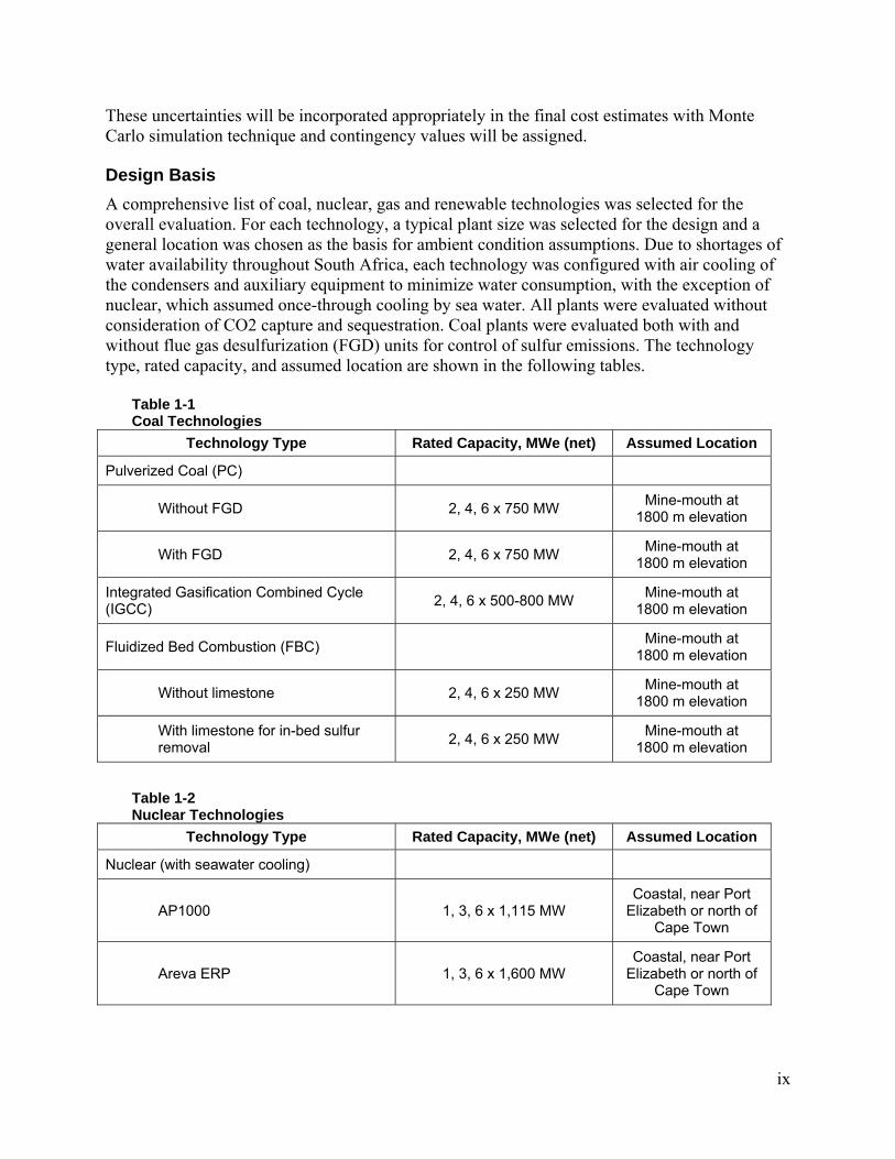
Design Basis A comprehensive list of coal, nuclear, gas and renewable technologies was selected for the overall evaluation. For each technology, a typical plant size was selected for the design and a general location was chosen as the basis for ambient condition assumptions. Due to shortages of water availability throughout South Africa, each technology was configured with air cooling of the condensers and auxiliary equipment to minimize water consumption, with the exception of nuclear, which assumed once-through cooling by sea water. All plants were evaluated without consideration of CO2 capture and sequestration. Coal plants were evaluated both with and without flue gas desulfurization (FGD) units for control of sulfur emissions. The technology type, rated capacity, and assumed location are shown in the following tables.
Table 1-1 Coal Technologies
Technology Type Rated Capacity, MWe (net) Assumed Location
Pulverized Coal (PC)
Without FGD 2, 4, 6 x 750 MW Mine-mouth at 1800 m elevation
With FGD 2, 4, 6 x 750 MW Mine-mouth at 1800 m elevation
Integrated Gasification Combined Cycle (IGCC) 2, 4, 6 x 500-800 MW Mine-mouth at
1800 m elevation
Fluidized Bed Combustion (FBC) Mine-mouth at 1800 m elevation
Without limestone 2, 4, 6 x 250 MW Mine-mouth at 1800 m elevation
With limestone for in-bed sulfur removal 2, 4, 6 x 250 MW Mine-mouth at
1800 m elevation
Table 1-2 Nuclear Technologies
Technology Type Rated Capacity, MWe (net) Assumed Location
Nuclear (with seawater cooling)
AP1000 1, 3, 6 x 1,115 MW Coastal, near Port
Elizabeth or north of Cape Town
Areva ERP 1, 3, 6 x 1,600 MW Coastal, near Port
Elizabeth or north of Cape Town
ix

Table 1-3 Gas Technologies
Technology Type Rated Capacity, MWe (net) Assumed Location
Combined Cycle Gas Turbine (CCGT) 500-800 MW Coastal, LNG based
Open Cycle Gas Turbine (OCGT) 100-190 MW Coastal, LNG based Table 1-4 Renewable Technologies
Technology Type Rated Capacity, MWe (net) Assumed Location
Wind 20, 50, 100, 200 MW Coastal
Parabolic Trough
Without storage 125 MW Upington
With indirect storage 125 MW Upington
Central Receiver
With direct storage 100, 125 MW Upington
Photovoltaics
Thin Film – rooftop 0.25, 1 MW Johannesburg and Cape Town
Thin Film – ground mounted 1, 10 MW Johannesburg and Cape Town
Concentrating 10 MW Upington
Biomass
Forestry Residue 25 MW Eastern coast
Municipal Solid Waste 25 MW Major cities
Landfill Gas Engines 5 MW Major cities
For this study, the coal technologies and biomass units were all considered to be baseload units with an 85% capacity factor while nuclear was assumed to have a 90% capacity factor. The combined cycle gas turbine was assumed to be an intermediate unit with a capacity factor of 50% and the simple cycle gas turbine unit was assumed to be a peaking unit with a capacity factor of 10%. The capacity factor of the renewable technologies, other than biomass, was determined based on the solar or wind resource available at the assumed location.
Capital Cost Estimating Basis Cost estimates were developed for each technology evaluated in this report. Total plant cost (TPC) and operation and maintenance (O&M) costs are presented as “overnight costs”, which assume that the plant is built overnight and, thus does not include interest and financing costs. All costs are expressed in January 2010 South African Rand (ZAR). Total plant costs were estimated by EPRI using a combination of in-house data and adjustment factors developed by EPRI’s subcontractor. Recent EPRI studies were used as a baseline for the cost estimates. These
x

estimates were adjusted as necessary to match the design basis for the current study by adjusting the size of the plant, including dry cooling, utilizing the proper fuel type when applicable, and modifying estimates for the specified ambient conditions. Based on current market trends, these baseline estimates were then adjusted to January 2010 US dollars (USD) as necessary.
Once capital and O&M costs were established for a US based plant with the same design as the design basis in January 2010, cost estimates were adjusted to determine how much it would cost to build the same plant in South Africa, based on assumptions about what percentage of the plant cost would be built using local labor, materials, and equipment vs. imported labor, materials, and equipment and by using the adjustment factors developed by EPRI’s subcontractor and in-house EPRI assumptions. Finally, these costs were converted to ZAR using an exchange rate of 7.4 ZAR per US dollar, based on the exchange rate between US dollars and the South African Rand at the beginning of January, 2010.
The flow diagram below shows the cost estimating approach graphically.
xi

TPC x % local
Local labor x labor factor
Local x % labor
Adjustment to design basis conditions
Adjustment to January 2010 costs
TPC x % imported
Local materials x materials factor
Imported x foreign factor
TPC and O&M x USD to ZAR conversion
Total Plant Cost and O&M Costs from recent EPRI study
in study year and USD
Total Plant Cost and O&M Costs for South African design
basis in study year USD
Total Plant Cost and O&M Costs for South African design
basis in January 2010 USD
Percentage of cost for local materials, equipment, and
labor
Percentage of costs for imported materials, equipment,
and labor
Local x % materials
Percentage of local cost for materials and
equipment
Percentage of local cost for labor
Adjusted local material and
equipment costs for South African
Adjusted local material and
equipment costs for South African
Adjusted imported cost for South African
construction
construction construction
Total Plant Cost and O&M Costs for imported and local equipment, materials, and labor
Total Plant Cost and O&M Costs in ZAR (1 USD = 7.4 ZAR)
xii

Results The following tables provide a summary of the cost and performance results from this study.
Table 1-5 Pulverized Coal without FGD Cost and Performance Summary
Technology 2x750 MW, No FGD
4x750 MW, No FGD
6x750 MW, No FGD
Rated Capacity, MW gross 1,599 3,197 4,796 Rated Capacity, MW net 1,500 3,000 4,500 Plant Cost Estimates (January 2010) Total Plant Cost, Overnight, ZAR/kW 16,880 16,025 15,470 Lead Times and Project Schedule, years 5 7 9 Single Unit Expense Schedule, % of TPC
per year 10%, 25%, 45%, 20%
10%, 25%, 45%, 20%
10%, 25%, 45%, 20%
Full Project Expense Schedule, % of TPC per year (* indicates commissioning year of first unit)
5%, 18%, 35%, 32%*,
10%
3%, 9%, 20%, 25%*, 22%, 16%,
5%
2%, 6%, 13%, 17%*, 17%, 16%, 15%, 11%,
3% Fuel Cost Estimates First Year, ZAR/GJ 15 15 15 Expected Escalation (beyond inflation) 0% 0% 0% Fuel Energy Content, HHV, kJ/kg 19,220 19,220 19,220 Operation and Maintenance Cost Estimates Fixed O&M, ZAR/kW-yr 379 360 348 Variable O&M, ZAR/MWh 36.3 36.3 36.3 Availability Estimates Equivalent Availability 91.7 91.7 91.7 Maintenance 4.8 4.8 4.8 Unplanned Outages 3.7 3.7 3.7 Performance Estimates Economic Life, years 30 30 30 Heat Rate, kJ/kWh Average Annual 9,643 9,643 9,643 100% Load 9,611 9,611 9,611 75% Load 9,779 9,779 9,779 50% Load 10,296 10,296 10,296 25% Load 12,349 12,349 12,349 Plant Load Factor Typical Capacity Factor 85% 85% 85% Maximum of Rated Capacity 100% 100% 100% Minimum of Rated Capacity 25% 25% 25% Water Usage
xiii

Per Unit of Energy, L/MWh 33.3 33.3 33.3 Sorbent (Limestone) Usage Per Unit of Energy, kg/MWh 0 0 0 Air Emissions, kg/MWh CO2 924.4 924.4 924.4 SOx 8.93 8.93 8.93 NOx 2.26 2.26 2.26 Hg 1.22E-06 1.22E-06 1.22E-06 Particulates 0.12 0.12 0.12 Solid Wastes kg/MWh FGD solids 0 0 0 Fly ash 166.4 166.4 166.4 Bottom ash 3.28 3.28 3.28
Table 1-6 Pulverized Coal with FGD Cost and Performance Summary
Technology 2x750 MW, With FGD
4x750 MW, With FGD
6x750 MW, With FGD
Rated Capacity, MW gross 1,619 3,237 4,856 Rated Capacity, MW net 1,500 3,000 4,500 Plant Cost Estimates (January 2010) Total Plant Cost, Overnight, ZAR/kW 19,655 18,455 17,785 Lead Times and Project Schedule, years 5 7 9 Single Unit Expense Schedule, % of TPC
per year 10%, 25%, 45%, 20%
10%, 25%, 45%, 20%
10%, 25%, 45%, 20%
Full Project Expense Schedule, % of TPC per year (* indicates commissioning year of first unit)
5%, 18%, 35%, 32%*,
10%
3%, 9%, 20%, 25%*, 22%, 16%,
5%
2%, 6%, 13%, 17%*, 17%, 16%, 15%, 11%,
3% Fuel Cost Estimates First Year, ZAR/GJ 15 15 15 Expected Escalation (beyond inflation) 0% 0% 0% Fuel Energy Content, HHV, kJ/kg 19,220 19,220 19,220 Operation and Maintenance Cost Estimates Fixed O&M, ZAR/kW-yr 502 472 455 Variable O&M, ZAR/MWh 44.4 44.4 44.4 Availability Estimates Equivalent Availability 91.7 91.7 91.7 Maintenance 4.8 4.8 4.8 Unplanned Outages 3.7 3.7 3.7 Performance Estimates Economic Life, years 30 30 30 Heat Rate, kJ/kWh Average Annual 9,769 9,769 9,769 100% Load 9,727 9,727 9,727
xiv

75% Load 9,913 9,913 9,913 50% Load 10,462 10,462 10,462 25% Load 12,716 12,716 12,716 Plant Load Factor Typical Capacity Factor 85% 85% 85% Maximum of Rated Capacity 100% 100% 100% Minimum of Rated Capacity 25% 25% 25% Water Usage Per Unit of Energy, L/MWh 229.1 229.1 229.1 Sorbent (Limestone) Usage Per Unit of Energy, kg/MWh 15.2 15.2 15.2 Air Emissions, kg/MWh CO2 936.2 936.2 936.2 SOx 0.45 0.45 0.45 NOx 2.30 2.30 2.30 Hg 1.27E-06 1.27E-06 1.27E-06 Particulates 0.13 0.13 0.13 Solid Wastes kg/MWh FGD solids 24.1 24.1 24.1 Fly ash 168.5 168.5 168.5 Bottom ash 3.32 3.32 3.32
Table 1-7 Integrated Gasification Combined Cycle Cost and Performance Summary
Technology Two 2x2x1 Shell IGCC
Four 2x2x1 Shell IGCC
Six 2x2x1 Shell IGCC
Rated Capacity, MW gross 1,578 3,157 4,735 Rated Capacity, MW net 1,288 2,577 3,865 Plant Cost Estimates (January 2010) Total Plant Cost, Overnight, ZAR/kW 24,670 23,160 22,325 Lead Times and Project Schedule, years 5 7 9 Single Unit Expense Schedule, % of TPC
per year 10%, 25%, 45%, 20%
10%, 25%, 45%, 20%
10%, 25%, 45%, 20%
Full Project Expense Schedule, % of TPC per year (* indicates commissioning year of first unit)
5%, 18%, 35%, 32%*,
10%
3%, 9%, 20%, 25%*, 22%, 16%,
5%
2%, 6%, 13%, 17%*, 17%, 16%, 15%, 11%,
3% Fuel Cost Estimates First Year, ZAR/GJ 15 15 15 Expected Escalation (beyond inflation) 0% 0% 0% Fuel Energy Content, kJ/kg 19,220 19,220 19,220 Operation and Maintenance Cost Estimates Fixed O&M, ZAR/kW-yr 830 779 751 Variable O&M, ZAR/MWh 14.4 14.4 14.4 Availability Estimates
xv

Equivalent Availability 85.7 85.7 85.7 Maintenance 4.7 4.7 4.7 Unplanned Outages 10.1 10.1 10.1 Performance Estimates Economic Life, years 30 30 30 Heat Rate, kJ/kWh Average Annual 9,758 9,758 9,758 100% Load 9,652 9,652 9,652 75% Load 10,328 10,328 10,328 50% Load* 12,258 12,258 12,258 25% Load -- -- -- Plant Load Factor Typical Capacity Factor 85% 85% 85% Maximum of Rated Capacity 100% 100% 100% Minimum of Rated Capacity 50% 50% 50% Water Usage Per Unit of Energy, L/MWh 256.8 256.8 256.8 Air Emissions, kg/MWh CO2 857.1 857.1 857.1 SOx (as SO2) 0.21 0.21 0.21 NOx (as NO2) 0.01 0.01 0.01 Solid Wastes kg/MWh Fly ash 9.7 9.7 9.7 Bottom ash 79.8 79.8 79.8 * The heat rate penalty could be mitigated by designing for approximately 50% load on the gasification/ASU system and turn off of one gas turbine.
Table 1-8 Fluidized Bed without FGD Cost and Performance Summary
Technology 2x250 MW, No FGD
4x250 MW, No FGD
6x250 MW, No FGD
Rated Capacity, MW gross 532 1,065 1,597 Rated Capacity, MW net 500 1,000 1,500 Plant Cost Estimates (January 2010) Total Plant Cost, Overnight, ZAR/kW 16,400 15,395 14,840 Lead Times and Project Schedule, years 5 7 9 Single Unit Expense Schedule, % of TPC
per year 10%, 25%, 45%, 20%
10%, 25%, 45%, 20%
10%, 25%, 45%, 20%
Full Project Expense Schedule, % of TPC per year (* indicates commissioning year of first unit)
5%, 18%, 35%, 32%*,
10%
3%, 9%, 20%, 25%*, 22%, 16%,
5%
2%, 6%, 13%, 17%*, 17%, 16%, 15%, 11%,
3% Fuel Cost Estimates
xvi

First Year, ZAR/GJ 15 15 15 Expected Escalation (beyond inflation) 0% 0% 0% Fuel Energy Content, kJ/kg 19,220 19,220 19,220 Operation and Maintenance Cost Estimates Fixed O&M, ZAR/kW-yr 402 378 364 Variable O&M, ZAR/MWh 69.1 69.1 69.1 Availability Estimates Equivalent Availability 90.4 90.4 90.4 Maintenance 5.7 5.7 5.7 Unplanned Outages 4.1 4.1 4.1 Performance Estimates Economic Life, years 30 30 30 Heat Rate, kJ/kWh Average Annual 10,060 10,060 10,060 100% Load 10,028 10,028 10,028 75% Load 10,202 10,202 10,202 50% Load 10,735 10,735 10,735 25% Load 12,858 12,858 12,858 Plant Load Factor Typical Capacity Factor 85% 85% 85% Maximum of Rated Capacity 100% 100% 100% Minimum of Rated Capacity 25% 25% 25% Water Usage Per Unit of Energy, L/MWh 33.3 33.3 33.3 Sorbent (Limestone) Usage Per Unit of Energy, kg/MWh 0 0 0 Air Emissions, kg/MWh CO2 959.5 959.5 959.5 SOx (as SO2) 9.36 9.36 9.36 NOx (as NO2) 0.20 0.20 0.20 Hg 0 0 0 Particulates 0.09 0.09 0.09 Solid Wastes kg/MWh Gypsum 0 0 0 Fly ash 35.1 35.1 35.1 Bottom ash 140.53 140.53 140.53
Table 1-9 Fluidized Bed with FGD Cost and Performance Summary
Technology 2x250 MW, With FGD
4x250 MW, With FGD
6x250 MW, With FGD
Rated Capacity, MW gross 534 1,067 1,601 Rated Capacity, MW net 500 1,000 1,500 Plant Cost Estimates (January 2010)
xvii

Total Plant Cost, Overnight, ZAR/kW 16,540 15,530 14,965 Lead Times and Project Schedule, years 5 7 9 Single Unit Expense Schedule, % of TPC
per year 10%, 25%, 45%, 20%
10%, 25%, 45%, 20%
10%, 25%, 45%, 20%
Full Project Expense Schedule, % of TPC per year (* indicates commissioning year of first unit)
5%, 18%, 35%, 32%*,
10%
3%, 9%, 20%, 25%*, 22%, 16%,
5%
2%, 6%, 13%, 17%*, 17%, 16%, 15%, 11%,
3% Fuel Cost Estimates First Year, ZAR/GJ 15 15 15 Expected Escalation (beyond inflation) 0% 0% 0% Fuel Energy Content, kJ/kg 19,220 19,220 19,220 Operation and Maintenance Cost Estimates Fixed O&M, ZAR/kW-yr 404 379 365 Variable O&M, ZAR/MWh 99.1 99.1 99.1 Availability Estimates Equivalent Availability 90.4 90.4 90.4 Maintenance 5.7 5.7 5.7 Unplanned Outages 4.1 4.1 4.1 Performance Estimates Economic Life, years 30 30 30 Heat Rate, kJ/kWh Average Annual 10,081 10,081 10,081 100% Load 10,048 10,048 10,048 75% Load 10,222 10,222 10,222 50% Load 10,756 10,756 10,756 25% Load 12,884 12,884 12,884 Plant Load Factor Typical Capacity Factor 85% 85% 85% Maximum of Rated Capacity 100% 100% 100% Minimum of Rated Capacity 25% 25% 25% Water Usage Per Unit of Energy, L/MWh 33.3 33.3 33.3 Sorbent (Limestone) Usage Per Unit of Energy, kg/MWh 28.4 28.4 28.4 Air Emissions, kg/MWh CO2 976.9 976.9 976.9 SOx (as SO2) 0.19 0.19 0.19 NOx (as NO2) 0.20 0.20 0.20 Hg 0 0 0 Particulates 0.09 0.09 0.09 Solid Wastes kg/MWh Gypsum 62.9 62.9 62.9 Fly ash 35.1 35.1 35.1
xviii

Bottom ash 140.53 140.53 140.53
Table 1-10 Nuclear Areva EPR Technology Performance and Cost Summary
Technology 1 Unit 3 Units 6 Units Rated Capacity, MW net 1,600 4,800 9,600 Plant Cost Estimates (January 2010) Total Plant Cost, Overnight, ZAR/kW 28,290 27,605 26,575 Lead Times and Project Schedule, years 6 10 16
Single Unit Expense Schedule, % of TPC per year
15%, 15%, 25%, 25%, 10%, 10%
15%, 15%, 25%, 25%, 10%, 10%
15%, 15%, 25%, 25%, 10%, 10%
Full Project Expense Schedule, % of TPC per year (* indicates commissioning year of first unit)
15%, 15%, 25%, 25%, 10%, 10%*
5%, 5%, 13%, 13%, 17%, 17%*, 12%, 12%,
3%, 3%
3%, 3%, 7%, 7%, 8%, 8%*, 8%, 8%, 8%, 8%, 8%, 8%, 6%, 6%, 2%,
2% Fuel Cost Estimates First Year, ZAR/GJ 6.25 6.25 6.25 Expected Escalation (beyond inflation) 0% 0% 0% Fuel Energy Content, GJ/kg 3,900 3,900 3,900 Operation and Maintenance Cost Estimates O&M, ZAR/MWh 99.6 97.3 95.2 Availability Estimates Equivalent Availability 92-95% 92-95% 92-95% Maintenance N/A N/A N/A Unplanned Outages <2% <2% <2% Performance Estimates Economic Life, years 60 60 60 Heat Rate, kJ/kWh 10,760 10,760 10,760 Water Usage Cooling (once-through sea water), L/MWh 6,000 6,000 6,000 Boiler Makeup, L/MWh Negligible Negligible Negligible
Table 1-11 Nuclear AP1000 Technology Performance and Cost Summary
Technology 1 Unit 3 Units 6 Units Rated Capacity, MW net 1,200 3,600 7,200 Plant Cost Estimates (January 2010) Total Plant Cost, Overnight, ZAR/kW 33,250 32,440 31,215 Lead Times and Project Schedule, years 6 10 16
Single Unit Expense Schedule, % of TPC per year
15%, 15%, 25%, 25%, 10%, 10%
15%, 15%, 25%, 25%, 10%, 10%
15%, 15%, 25%, 25%, 10%, 10%
xix

Full Project Expense Schedule, % of TPC per year (* indicates commissioning year of first unit)
15%, 15%, 25%, 25%, 10%, 10%*
5%, 5%, 13%, 13%, 17%, 17%*, 12%, 12%,
3%, 3%
3%, 3%, 7%, 7%, 8%, 8%*, 8%, 8%, 8%, 8%, 8%, 8%, 6%, 6%, 2%,
2% Fuel Cost Estimates First Year, ZAR/GJ 6.25 6.25 6.25 Expected Escalation (beyond inflation) 0% 0% 0% Fuel Energy Content, GJ/kg 3,900 3,900 3,900 Operation and Maintenance Cost Estimates O&M, ZAR/MWh 124.4 121.1 118.1 Availability Estimates Equivalent Availability 93% 93% 93% Maintenance 2.8-3% 2.8-3% 2.8-3% Unplanned Outages 4% 4% 4% Performance Estimates Economic Life, years 60 60 60 Heat Rate, kJ/kWh 10,250 10,250 10,250 Water Usage Cooling (once-through sea water), L/MWh 6,000 6,000 6,000 Boiler Makeup, L/MWh Negligible Negligible Negligible
Table 1-12 Gas Turbine Cost and Performance Summary
Technology Open Cycle
Gas Turbine
Combined Cycle Gas
Turbine Rated Capacity, MW gross 115.9 732.4 Rated Capacity, MW net 114.7 711.3 Plant Cost Estimates (January 2010) Total Plant Cost, Overnight, ZAR/kW 3,955 5,780 Lead Times and Project Schedule, years 2 3
Expense Schedule, % of TPC per year 90%, 10% 40%, 50%, 10%
Fuel Cost Estimates First Year, ZAR/GJ 42.1 42.1
Expected Escalation (beyond inflation) See discussion in Gas Turbine section
Fuel Energy Content, MJ/SCM 39.3 39.3 Operation and Maintenance Cost Estimates Fixed O&M, ZAR/kW-yr 70 148 Variable O&M, ZAR/MWh 0.0 0.0 Availability Estimates Equivalent Availability 88.8 88.8
xx

Maintenance 6.9 6.9 Unplanned Outages 4.6 4.6 Performance Estimates Economic Life, years 30 30 Heat Rate, kJ/kWh Average Annual 11,926 7,486 100% Load 10,841 7,269 75% Load 11,622 7,817 50% Load 13,236 7,941 25% Load 18,227 8,388 Plant Load Factor Typical Capacity Factor 10% 50% Maximum of Rated Capacity 100% 100% Minimum of Rated Capacity 20% 20% Water Usage Per Unit of Energy, L/MWh 19.8 12.8 Air Emissions, kg/MWh CO2 622 376 SOx (as SO2) 0 0 NOx (as NO2) 0.28 0.29 Hg 0 0 Particulates 0 0
Table 1-13 Wind Technology Performance and Cost Summary
Technology 10 x 2 MW 25 x 2 MW 50 x 2 MW 100 x 2 MWRated Capacity, MW net 20 50 100 200 Plant Cost Estimates (January 2010) Total Plant Cost, Overnight, ZAR/kW 16,930 15,890 15,150 14,445 Lead Times and Project Schedule, years 2-3.5 2.5-4 3-5 3-6
Expense Schedule, % of TPC per year 5%, 5%, 90%
2.5%, 2.5%, 5%, 90%
5%, 5%, 10%, 80%
2.5%, 2.5%, 5%, 15%,
75% Operation and Maintenance Cost Estimates Fixed O&M, ZAR/kW-yr 312 293 279 266 Availability Estimates 94-97% 94-97% 94-97% 94-97% Performance Estimates Economic Life, years 20 20 20 20 Capacity Factor See Table 1-14
Table 1-14 Wind Turbine Capacity Factors
Wind Class 3 4 5 6 Average Wind Speed (m/s @ 10-meter measurement height) 5.3 5.8 6.2 6.7
xxi

Average Wind Speed (m/s @ 80-meter hub height) 7.2 7.8 8.3 9
Net Capacity Factor, % 29.1 33.2 36.6 40.6
Table 1-15 Parabolic Trough Cost and Performance Summary
Technology 0 Hours Storage
3 Hours Storage
6 Hours Storage
9 Hours Storage
Rated Capacity, MW net 125 125 125 125 Plant Cost Estimates (January 2010) Total Plant Cost, Overnight, ZAR/kW 27,450 37,425 43,385 50,910 Lead Times and Project Schedule, years 4 4 4 4
Expense Schedule, % of TPC per year 10%, 25%, 45%, 20%
10%, 25%, 45%, 20%
10%, 25%, 45%, 20%
10%, 25%, 45%, 20%
Operation and Maintenance Cost Estimates Fixed O&M, ZAR/kW-yr 424 513 562 635 Availability Estimates 95% 95% 95% 95% Performance Estimates Economic Life, years 30 30 30 30 Solar to Electric Efficiency 13.3% 13.2% 13.5% 13.6% Capacity Factor (in Upington, SA) 25.0% 31.2% 36.3% 43.7% Water Usage Per Unit of Energy, L/MWh 270 250 245 245
Table 1-16 Central Receiver Cost and Performance Summary
Technology 3 Hours Storage
6 Hours Storage
9 Hours Storage
12 Hours Storage
14 Hours Storage
Rated Capacity, MW net 125 125 125 100 100 Plant Cost Estimates (January 2010) Total Plant Cost, Overnight, ZAR/kW 26,910 32,190 36,225 39,025 40,200 Lead Times and Project Schedule, years 4 4 4 4 4
Expense Schedule, % of TPC per year
10%, 25%, 45%, 20%
10%, 25%, 45%, 20%
10%, 25%, 45%, 20%
10%, 25%, 45%, 20%
10%, 25%, 45%, 20%
Operation and Maintenance Cost Estimates Fixed O&M, ZAR/kW-yr 489 546 603 660 701 Availability Estimates 92% 92% 92% 92% 92% Performance Estimates Economic Life, years 30 30 30 30 30 Solar to Electric Efficiency 16.2% 15.9% 15.8% N/A N/A Capacity Factor (in Upington, SA) 29.2% 36.7% 41.0% 46.8% 47.6% Water Usage Per Unit of Energy, L/MWh 280 295 315 305 316
xxii

Table 1-17 CdTe PV Cost and Performance Summary
Technology Thin Film Fixed Tilt CdTe Mounting Location Rooftop (0° tilt) Ground (latitudinal tilt) Rated Capacity, MW net 0.25 1 1 10 Plant Cost Estimates (January 2010) Total Plant Cost, Overnight, ZAR/kW 42,020 34,200 36,000 28,055 Lead Times and Project Schedule, years 1 1 2 2 Expense Schedule, % of TPC per year 100% 100% 10%, 90% 10%, 90% Operation and Maintenance Cost Estimates Fixed O&M, ZAR/kW-yr 402 402 402 402 Availability Estimates 98% 98% 98% 98% Performance Estimates Economic Life, years 25 25 25 25 Capacity Factor See Table 1-20Water Usage, L/yr 11,270 45,080 45,080 450,800
Table 1-18 Amorphous Silicon PV Cost and Performance Summary
Technology Thin Film Fixed Tilt a-Si Mounting Location Rooftop (0° tilt) Ground (latitudinal tilt) Rated Capacity, MW net 0.25 1 1 10 Plant Cost Estimates (January 2010) Total Plant Cost, Overnight, ZAR/kW 43,400 35,250 37,095 28,910 Lead Times and Project Schedule, years 1 1 2 2 Expense Schedule, % of TPC per year 100% 100% 10%, 90% 10%, 90% Operation and Maintenance Cost Estimates Fixed O&M, ZAR/kW-yr 402 402 402 402 Availability Estimates 98% 98% 98% 98% Performance Estimates Economic Life, years 25 25 25 25 Capacity Factor See Table 1-20Water Usage, L/yr 8,480 33,935 33,935 339,350
Table 1-19 Concentrating PV Cost and Performance Summary
Technology Concentrating PV
Rated Capacity, MW net 10 Plant Cost Estimates (January 2010) Total Plant Cost, Overnight, ZAR/kW 37,225 Lead Times and Project Schedule, years 2
xxiii

Expense Schedule, % of TPC per year 10%, 90% Operation and Maintenance Cost Estimates Fixed O&M, ZAR/kW-yr 502 Availability Estimates 95% Performance Estimates Economic Life, years 25 Capacity Factor (1st Year) 29.1% Capacity Factor (Average) 26.8% Water Usage, L /yr 395,890
Table 1-20 Thin Film PV Capacity Factors
Technology CdTe a-Si
Mounting Location Rooftop (0° tilt) Ground (latitudinal tilt) Rooftop (0° tilt) Ground
(latitudinal tilt) Cape Town (1st Year) 18.7% 20.7% 18.7% 20.7% Cape Town (Average) 17.0% 18.8% 17.0% 18.9% Johannesburg (1st Year) 19.4% 21.4% 19.4% 21.4% Johannesburg (Average) 17.6% 19.4% 17.6% 19.4%
Table 1-21 Biomass Cost and Performance Summary
Technology Forestry Residue
Municipal Solid Waste
Rated Capacity, MW net 25 25 Plant Cost Estimates (January 2010) Total Plant Cost, Overnight, ZAR/kW 33,270 66,900 Lead Times and Project Schedule, years 3.5-4 3.5-4
Expense Schedule, % of TPC per year 10%, 25%, 45%, 20%
10%, 25%, 45%, 20%
Fuel Cost Estimates First Year, ZAR/GJ 19.5 0 Expected Escalation (beyond inflation) 0% 0% Fuel Energy Content, kJ/kg 11,760 11,390 Operation and Maintenance Cost Estimates Fixed O&M, ZAR/kW-yr 972 2,579 Variable O&M, ZAR/MWh 31.1 38.2 Availability Estimates Equivalent Availability 90% 90% Maintenance 4% 4% Unplanned Outages 6% 6% Performance Estimates Economic Life, years 30 30 Heat Rate, kJ/kWh 14,185 18,580 Plant Load Factor
xxiv

Typical Capacity Factor 85% 85% Maximum of Rated Capacity 100% 100% Minimum of Rated Capacity 40% 40% Water Usage Per Unit of Energy, L/MWh 210 200 Air Emissions, kg/MWh CO2 1287 1607 SOx (as SO2) 0.78 0.56 NOx (as NO2) 0.61 0.80 CO 1.52 2.00 Particulates 0.16 0.28 HCl 0.00 0.22 Solid Wastes kg/MWh Fly ash 24.2 1226 Bottom ash 6.1 3000
xxv


CONTENTS
1 INTRODUCTION ....................................................................................................................1-1 Introduction ...........................................................................................................................1-1
Objectives .............................................................................................................................1-2
Task Descriptions..................................................................................................................1-3
2 BACKGROUND AND GENERAL APPROACH.....................................................................2-1 Introduction ...........................................................................................................................2-1
3 DESIGN BASIS ......................................................................................................................3-1 Introduction ...........................................................................................................................3-1
Coal Technologies.................................................................................................................3-1
Location ............................................................................................................................3-1
Ambient Conditions ..........................................................................................................3-1
Duty Cycle ........................................................................................................................3-1
Generating Unit Size ........................................................................................................3-2
Cost Boundary..................................................................................................................3-2
Fuel Systems....................................................................................................................3-2
Resource Potential ...........................................................................................................3-3
Other Factors....................................................................................................................3-5
CO2 Capture and Storage ...........................................................................................3-5
Emissions Criteria........................................................................................................3-5
Dry Cooling ..................................................................................................................3-5
Ash Handling ...............................................................................................................3-5
Nuclear Technologies............................................................................................................3-5
Location ............................................................................................................................3-5
Duty Cycle ........................................................................................................................3-5
Generating Unit Size ........................................................................................................3-5
Cost Boundary..................................................................................................................3-6
xxvii

Resource Potential ...........................................................................................................3-6
Other Factors....................................................................................................................3-6
Once-Through Cooling.................................................................................................3-6
Gas Technologies .................................................................................................................3-6
Ambient Conditions ..........................................................................................................3-6
Duty Cycle ........................................................................................................................3-7
Generating Unit Size ........................................................................................................3-7
Cost Boundary..................................................................................................................3-7
Fuel Systems....................................................................................................................3-8
Resource Potential ...........................................................................................................3-8
Other Factors....................................................................................................................3-8
CO2 Capture and Storage ...........................................................................................3-8
Dry Cooling ..................................................................................................................3-9
Renewable Technologies......................................................................................................3-9
Wind Turbines ..................................................................................................................3-9
Location .......................................................................................................................3-9
Generating Unit Size....................................................................................................3-9
Cost Boundary .............................................................................................................3-9
Resource Potential ......................................................................................................3-9
Solar Thermal .................................................................................................................3-11
Location .....................................................................................................................3-11
Ambient Conditions....................................................................................................3-11
Generating Unit Size..................................................................................................3-12
Cost Boundary ...........................................................................................................3-12
Resource Potential ....................................................................................................3-12
Solar Photovoltaics.........................................................................................................3-14
Location .....................................................................................................................3-14
Ambient Conditions....................................................................................................3-14
Generating Unit Size..................................................................................................3-15
Cost Boundary ...........................................................................................................3-15
Resource Potential ....................................................................................................3-15
Biomass..........................................................................................................................3-17
Location .....................................................................................................................3-17
Generating Unit Size..................................................................................................3-18
Cost Boundary ...........................................................................................................3-18
xxviii

Fuel Systems .............................................................................................................3-18
Resource Potential ....................................................................................................3-19
Availability Estimates...........................................................................................................3-19
4 CAPITAL COST ESTIMATING BASIS ..................................................................................4-1 Baseline Cost Estimating Methodology.................................................................................4-1
Adjustments to Costs ............................................................................................................4-2
Adjustments to South African Construction Costs............................................................4-2
Adjustments to Operation and Maintenance Costs ..........................................................4-6
Total Capital Required Calculations ......................................................................................4-6
Preproduction Costs .........................................................................................................4-6
Inventory Capital...............................................................................................................4-7
Fleet Strategy........................................................................................................................4-7
Cost and Performance Data Uncertainties..........................................................................4-11
Sensitivity Analysis..............................................................................................................4-14
5 COST OF ELECTRICITY METHODOLOGY..........................................................................5-1 Introduction ...........................................................................................................................5-1
The Components of Revenue Requirements ........................................................................5-2
An Overview .....................................................................................................................5-2
The Nature of Fixed Charges ...........................................................................................5-3
The Components of Fixed Charges..................................................................................5-3
Depreciation.................................................................................................................5-3
Return on Equity ..........................................................................................................5-4
Interest on Debt ...........................................................................................................5-4
Income Taxes ..............................................................................................................5-5
Property Taxes and Insurance.....................................................................................5-5
Calculating Annual Capital Revenue Requirements .............................................................5-5
Calculating Cost of Electricity................................................................................................5-8
Annual Megawatt-Hours Produced...................................................................................5-9
Constant vs. Current Dollars ............................................................................................5-9
Capital Contribution to Cost of Electricity .........................................................................5-9
O&M Contribution to Cost of Electricity ............................................................................5-9
Fuel Contribution to Cost of Electricity ...........................................................................5-10
Sensitivity to Financial Parameters .....................................................................................5-10
xxix

6 TECHNOLOGY DESCRIPTIONS...........................................................................................6-1 Coal Technologies.................................................................................................................6-1
Pulverized Coal (PC) ........................................................................................................6-1
Integrated Gasification Combined Cycle (IGCC)..............................................................6-3
Fluidized Bed Combustion (FBC) .....................................................................................6-6
Nuclear Technologies............................................................................................................6-8
Areva EPR........................................................................................................................6-9
Westinghouse AP1000 ...................................................................................................6-12
Gas Technologies ...............................................................................................................6-15
Combined Cycle Gas Turbine (CCGT)...........................................................................6-15
Open Cycle Gas Turbine ................................................................................................6-17
Renewable Technologies....................................................................................................6-19
Wind ...............................................................................................................................6-19
On-Shore Wind ..........................................................................................................6-20
Off-Shore Wind ..........................................................................................................6-22
Solar Thermal .................................................................................................................6-22
Parabolic Trough .......................................................................................................6-23
Central Receiver ........................................................................................................6-24
Solar Photovoltaic...........................................................................................................6-26
Thin-Film....................................................................................................................6-29
Concentrating PV.......................................................................................................6-30
Biomass..........................................................................................................................6-30
Forestry Residue........................................................................................................6-31
Municipal Solid Waste................................................................................................6-31
Landfill Gas................................................................................................................6-33
7 COAL TECHNOLOGIES PERFORMANCE AND COST .......................................................7-1 Pulverized Coal .....................................................................................................................7-1
Plant Cost Estimates ...................................................................................................7-3
Fuel Cost Estimates.....................................................................................................7-4
Operation and Maintenance Cost Estimates ...............................................................7-4
Availability and Performance Estimates.......................................................................7-4
Cost of Electricity .........................................................................................................7-4
Water Usage................................................................................................................7-5
Emissions ....................................................................................................................7-5
xxx

Integrated Gasification Combined Cycle ...............................................................................7-5
Plant Cost Estimates ...................................................................................................7-6
Fuel Cost Estimates.....................................................................................................7-7
Operation and Maintenance Cost Estimates ...............................................................7-7
Availability and Performance Estimates.......................................................................7-7
Cost of Electricity .........................................................................................................7-8
Water Usage................................................................................................................7-8
Emissions ....................................................................................................................7-8
Fluidized Bed Combustion ....................................................................................................7-9
Plant Cost Estimates .................................................................................................7-11
Fuel Cost Estimates...................................................................................................7-11
Operation and Maintenance Cost Estimates .............................................................7-11
Availability and Performance Estimates.....................................................................7-12
Cost of Electricity .......................................................................................................7-12
Water Usage..............................................................................................................7-13
Emissions ..................................................................................................................7-13
8 NUCLEAR TECHNOLOGY PERFORMANCE AND COST ...................................................8-1 Plant Cost Estimates.............................................................................................................8-2
Fuel Cost Estimates ..............................................................................................................8-3
Operation and Maintenance Cost Estimates.........................................................................8-3
Availability and Performance Estimates ................................................................................8-4
Cost of Electricity...................................................................................................................8-4
Water Usage .........................................................................................................................8-5
9 GAS TECHNOLOGIES PERFORMANCE AND COST .........................................................9-1 Plant Cost Estimates.............................................................................................................9-2
Fuel Cost Estimates ..............................................................................................................9-2
Operation and Maintenance Cost Estimates.........................................................................9-7
Availability and Performance Estimates ................................................................................9-7
Cost of Electricity...................................................................................................................9-7
Water Usage .........................................................................................................................9-7
Emissions..............................................................................................................................9-8
10 RENEWABLE TECHNOLOGIES PERFORMANCE AND COST ......................................10-1 Wind ....................................................................................................................................10-1
xxxi

Plant Cost Estimates .................................................................................................10-1
Operation and Maintenance Cost Estimates .............................................................10-1
Availability and Performance Estimates.....................................................................10-2
Cost of Electricity .......................................................................................................10-2
Solar Thermal......................................................................................................................10-3
Plant Cost Estimates .................................................................................................10-4
Operation and Maintenance Cost Estimates .............................................................10-5
Availability and Performance Estimates.....................................................................10-5
Cost of Electricity .......................................................................................................10-5
Water Usage..............................................................................................................10-6
Photovoltaics.......................................................................................................................10-6
Plant Cost Estimates .................................................................................................10-8
Operation and Maintenance Cost Estimates .............................................................10-8
Availability and Performance Estimates.....................................................................10-8
Cost of Electricity .......................................................................................................10-9
Water Usage............................................................................................................10-10
Biomass ............................................................................................................................10-10
Plant Cost Estimates ...............................................................................................10-12
Fuel Cost Estimates.................................................................................................10-13
Operation and Maintenance Cost Estimates ...........................................................10-14
Availability and Performance Estimates...................................................................10-14
Cost of Electricity .....................................................................................................10-15
Water Usage............................................................................................................10-15
Emissions ................................................................................................................10-15
11 GRID INTEGRATION AND INTERMITTENCY ISSUES FOR NON-THERMAL RENEWABLE TECHNOLOGIES ............................................................................................11-1
Technology Characteristics .................................................................................................11-2
Wind Integration Issues ..................................................................................................11-2
Photovoltaic Solar Integration Issues .............................................................................11-2
Integration issues ................................................................................................................11-3
Intermittency ...................................................................................................................11-3
Ramping Burdens...........................................................................................................11-3
Fluctuating Power Output ...............................................................................................11-4
Limited Reactive Power Control .....................................................................................11-4
xxxii

Distributed Generation....................................................................................................11-4
Remote Location of Some Renewable Resources.........................................................11-5
Integration Technologies for Distribution-Connected Renewable Generation ....................11-5
Integration Technologies for Transmission-Connected Renewable Generation .................11-7
Variable Generation Technical and Cost Challenges..........................................................11-7
Integration for Distribution-Connected Renewable Generation ......................................11-7
Integration for Transmission-Connected Renewable Generation...................................11-8
Grid Planning and Operating Tools ................................................................................11-9
References........................................................................................................................11-10
A ACRONYM LIST ................................................................................................................... A-1
B SOLAR GENERATION PROFILES...................................................................................... B-1
xxxiii


LIST OF FIGURES
Figure 3-1 South African Wind Resource (measured at 10 m) ................................................3-10 Figure 3-2 South African Wind Resource (measured at 10 m) (from Mesoscale Wind
Atlas of South Africa presented by Kilian Hagemann March 2009; www.crses.sun.ac.za/pdfs/Hagemann.pdf) ......................................................................3-11
Figure 3-3 Worldwide DNI Data ..............................................................................................3-13 Figure 3-4 African Annual Direct Normal Radiation .................................................................3-14 Figure 3-5 African Annual Latitudinal Solar Radiation .............................................................3-16 Figure 3-6 African Annual Horizontal Solar Radiation .............................................................3-17 Figure 3-7 Availability Definitions and Calculations .................................................................3-20 Figure 4-1 Coal Plant Six Unit Expense Schedule.....................................................................4-9 Figure 4-2 Nuclear Plant Six Unit Expense Schedule................................................................4-9 Figure 4-3 Nuclear Plant Six Year Total Expenditure Schedule ..............................................4-10 Figure 4-4 Nuclear Plant Six Year Expenditure and Revenue Required Schedule .................4-10 Figure 4-5 Labor Productivity Factor Distribution.....................................................................4-15 Figure 4-6 Cumulative Frequency for Total Plant Cost ...........................................................4-17 Figure 4-7 Variance Contribution .............................................................................................4-18 Figure 5-1 Revenue Categories for the Revenue Requirement Method of Economic
Comparison........................................................................................................................5-2 Figure 6-1 Simple Schematic of Pulverized Coal (Supercritical) Generating Unit .....................6-2 Figure 6-2 Schematic of an IGCC Power Plant .........................................................................6-4 Figure 6-3 Schematic of a Fluidized Bed Combustion Boiler system ........................................6-7 Figure 6-4 Example plant layout of the US EPR (provided by AREVA NP).............................6-12 Figure 6-5 Simplified process flow diagram for the EPR (provided by AREVA NP) ................6-12 Figure 6-6 Typical process flow diagram for a PWR................................................................6-14 Figure 6-7 AP1000 passive containment cooling system (provided by Westinghouse
Electric Co., LLC) .............................................................................................................6-15 Figure 6-8 Simple Schematic of CCGT....................................................................................6-16 Figure 6-9 Open Cycle Compressor Inlet Temperature Performance Curve...........................6-18 Figure 6-10 Open Cycle Altitude Correction Curve..................................................................6-19 Figure 6-11 Wind Turbine Front and Side View.......................................................................6-20 Figure 6-12 Parabolic Trough ..................................................................................................6-24 Figure 6-13 Parabolic Trough North-South Axis View .............................................................6-24 Figure 6-14 Picture of Central Receiver Plant .........................................................................6-25
xxxv

Figure 6-15 Heliostat to Receiver Sun Path.............................................................................6-25 Figure 6-16 Schematic of Molten-Salt Power Tower System ..................................................6-26 Figure 6-17 Conceptual Overview of Solar PV System ..........................................................6-28 Figure 9-1 Relative Transportation Costs – 2002 Perspective ..................................................9-3 Figure 9-2 Relative Transportation Costs – 2004 Perspective ..................................................9-4 Figure 9-3 Relative Transportation Costs – 2007 Perspective ..................................................9-4 Figure 10-1 Fuel Cost for MSW Based on Tipping Fee .........................................................10-14
xxxvi

LIST OF TABLES
Table 1-1 Coal Technologies ....................................................................................................... ix Table 1-2 Nuclear Technologies .................................................................................................. ix Table 1-3 Gas Technologies......................................................................................................... x Table 1-4 Renewable Technologies ............................................................................................. x Table 1-5 Pulverized Coal without FGD Cost and Performance Summary ................................xiii Table 1-6 Pulverized Coal with FGD Cost and Performance Summary .....................................xiv Table 1-7 Integrated Gasification Combined Cycle Cost and Performance Summary ............... xv Table 1-8 Fluidized Bed without FGD Cost and Performance Summary....................................xvi Table 1-9 Fluidized Bed with FGD Cost and Performance Summary........................................xvii Table 1-10 Nuclear Areva EPR Technology Performance and Cost Summary..........................xix Table 1-11 Nuclear AP1000 Technology Performance and Cost Summary...............................xix Table 1-12 Gas Turbine Cost and Performance Summary......................................................... xx Table 1-13 Wind Technology Performance and Cost Summary.................................................xxi Table 1-14 Wind Turbine Capacity Factors ................................................................................xxi Table 1-15 Parabolic Trough Cost and Performance Summary ................................................xxii Table 1-16 Central Receiver Cost and Performance Summary.................................................xxii Table 1-17 CdTe PV Cost and Performance Summary............................................................ xxiii Table 1-18 Amorphous Silicon PV Cost and Performance Summary....................................... xxiii Table 1-19 Concentrating PV Cost and Performance Summary .............................................. xxiii Table 1-20 Thin Film PV Capacity Factors ...............................................................................xxiv Table 1-21 Biomass Cost and Performance Summary.............................................................xxiv Table 2-1 Coal Technologies .....................................................................................................2-1 Table 2-2 Nuclear Technologies ................................................................................................2-2 Table 2-3 Gas Technologies......................................................................................................2-2 Table 2-4 Renewable Technologies ..........................................................................................2-2 Table 3-1 South African Coal Characteristics ............................................................................3-2 Table 3-2 Natural Gas Characteristics.......................................................................................3-8 Table 3-3 Wind Speed Classes .................................................................................................3-9 Table 3-4 Biomass Characteristics ..........................................................................................3-18 Table 3-5 Landfill Gas Characteristics .....................................................................................3-19 Table 4-1 US Gulf Coast to South Africa Construction Factors .................................................4-2 Table 4-2 Assumptions of Imported vs Local, Material vs Labor Percentages ..........................4-3
xxxvii

Table 4-3 Fuel and Consumables Inventory ..............................................................................4-7 Table 4-4 Confidence Rating Based on Technology Development Status .............................4-11 Table 4-5 Confidence Rating Based on Cost and Design Estimate ........................................4-11 Table 4-6 Accuracy Range Estimates for Cost Data (Ranges in Percent) ..............................4-12 Table 4-7 Probability Assumptions ..........................................................................................4-15 Table 4-8 Total Plant Cost Uncertainty Ranges.......................................................................4-15 Table 4-9 Average Sensitivity Analysis Results for All Technologies ......................................4-17 Table 4-10 Contribution to Variance for All Technologies........................................................4-18 Table 5-1 Economic Parameters ...............................................................................................5-1 Table 5-2 Book Lives and Book Depreciation for Utility Plant....................................................5-4 Table 5-3 Key Characteristics of Utility Securities .....................................................................5-5 Table 5-4 Annual Capital Revenue Requirements by Component ...........................................5-6 Table 5-5 Annual Fixed Charge Rate and Levelized Charge Rates .........................................5-7 Table 5-6 Sensitivity Economic Parameters ............................................................................5-10 Table 5-7 Sensitivity Cost of Electricity Results.......................................................................5-11 Table 7-1 Pulverized Coal without FGD Cost and Performance Summary ...............................7-1 Table 7-2 Pulverized Coal with FGD Cost and Performance Summary ....................................7-2 Table 7-3 Pulverized Coal without FGD Levelized Cost of Electricity........................................7-4 Table 7-4 Pulverized Coal with FGD Levelized Cost of Electricity.............................................7-5 Table 7-5 Integrated Gasification Combined Cycle Cost and Performance Summary ..............7-5 Table 7-6 IGCC Levelized Cost of Electricity.............................................................................7-8 Table 7-7 Fluidized Bed without FGD Cost and Performance Summary...................................7-9 Table 7-8 Fluidized Bed with FGD Cost and Performance Summary......................................7-10 Table 7-9 Fluidized Bed without FGD Levelized Cost of Electricity .........................................7-12 Table 7-10 Fluidized Bed with FGD Levelized Cost of Electricity ............................................7-12 Table 8-1 Nuclear Areva EPR Technology Performance and Cost Summary...........................8-1 Table 8-2 Nuclear AP1000 Technology Performance and Cost Summary................................8-1 Table 8-3 Nuclear Areva EPR Levelized Cost of Electricity.......................................................8-4 Table 8-4 Nuclear AP1000 Levelized Cost of Electricity............................................................8-4 Table 9-1 Gas Turbine Cost and Performance Summary..........................................................9-1 Table 9-2 Natural Gas and LNG Estimates ($/MMBtu)..............................................................9-6 Table 9-3 Natural Gas and LNG Estimates (ZAR/GJ) ...............................................................9-6 Table 9-4 Gas Turbine Levelized Cost of Electricity ..................................................................9-7 Table 10-1 Wind Technology Performance and Cost Summary..............................................10-1 Table 10-2 Wind Turbine Capacity Factors .............................................................................10-2 Table 10-3 Wind Levelized Cost of Electricity – 10 x 2 MW Farm ...........................................10-2 Table 10-4 Wind Levelized Cost of Electricity – 25 x 2 MW Farm ...........................................10-3 Table 10-5 Wind Levelized Cost of Electricity – 50 x 2 MW Farm ...........................................10-3 Table 10-6 Wind Levelized Cost of Electricity – 100 x 2 MW Farm .........................................10-3
xxxviii

Table 10-7 Parabolic Trough Cost and Performance Summary ..............................................10-3 Table 10-8 Central Receiver Cost and Performance Summary...............................................10-4 Table 10-9 Parabolic Trough Levelized Cost of Electricity ......................................................10-6 Table 10-10 Central Receiver Levelized Cost of Electricity .....................................................10-6 Table 10-11 CdTe PV Cost and Performance Summary.........................................................10-6 Table 10-12 Amorphous Silicon PV Cost and Performance Summary....................................10-7 Table 10-13 Concentrating PV Cost and Performance Summary ...........................................10-7 Table 10-14 Thin Film PV Capacity Factors ............................................................................10-9 Table 10-15 CdTe Levelized Cost of Electricity – Cape Town.................................................10-9 Table 10-16 a-Si Levelized Cost of Electricity – Cape Town ...................................................10-9 Table 10-17 CdTe Levelized Cost of Electricity – Johannesburg ............................................10-9 Table 10-18 a-Si Levelized Cost of Electricity – Johannesburg.............................................10-10 Table 10-19 CPV Levelized Cost of Electricity ......................................................................10-10 Table 10-20 Biomass Cost and Performance Summary........................................................10-10 Table 10-21 Landfill Gas Reciprocating Engine Cost and Performance Summary ...............10-11 Table 10-22 Biomass Levelized Cost of Electricity ................................................................10-15
xxxix


1 INTRODUCTION
Introduction The Department of Energy, South Africa is in the process of preparing an integrated resource plan (IRP). The DOE South Africa has stipulated that the data included in the IRP must be developed from an independent source. To obtain this independently sourced data, Electric Power Research Institute (EPRI) was approached to provide technology data for new power plants that would be included in their IRP.
Because the project requires a quick turn-around of cost and performance data for a number of power generation technologies applicable to South African conditions and environments, a comprehensive analysis developed with ground-up estimates was not feasible. However, estimates pertinent to South African conditions were developed based on a compilation of existing US and international databases and adjustments based on third party vendor indices and EPRI in-house expertise.
The scope of this report includes capital cost, operations and maintenance (O&M) cost, and performance data. A comprehensive discussion and description of each technology also is presented. Costs are reported in January 2010 South African Rand.
Even as the recession was significantly impacting most of the US economy in 2008 and 2009, prices of many power plant-related materials and equipment continued to increase into early 2009. While most sectors of the economy experienced recession and factory shutdowns, the existing contracts and heavy backlog from 2008 kept manufacturers and suppliers of power plant equipment operating at near peak capacity. Major equipment ordered in 2007 and 2008 with one year to two year lead times have kept power plant manufacturing facilities busy at least up to the present time. The growth in escalation rates in the power plant sector was sustained by the orders from 2007 and early 2008 for materials and equipment for new power plants; power plant emission control system retrofits; craft labor contracts negotiated in 2007 with 4% to 5% annual escalation clauses for 2008 (and in some cases for 2008 and 2009); and the multi-billion dollar refinery expansion projects.
There are mixed signs regarding utility power plant costs with significant declines in the price of steel plate and structural steel on the one hand and continuing escalation of major equipment on the other hand. The volatility of markets makes it difficult for utility personnel to keep up with the changes.
Because of the drastic change in economic scenario from the high cost escalation in 2004-2008 time period to a global (except in China and India) recession in 2009, the rationale for the costs presented in this report is as follows:
1-1

Introduction
• Estimates (constant January 2010) represent composite material and labor cost estimates from mid-2009.
• These values are expected to hold good for planning purposes for projects that would have a first year commercial service date in 2015-2020 time frame.
• The preliminary indications of a drop in escalation in the first and second quarter 2009 from published sources is expected to be a temporary phenomena and the price of commodities and labor is expected to revert back to December 2008 levels by the mid-late 2010.
• Project executions in the US are expected to revive in the fourth quarter 2010 and the on-going projects in cash rich China and India are expected to stabilize the 2008 year end price levels in late 2010.
The cost and performance estimates included in this report are based on conceptual level of effort idealized for representative generating units at appropriate South Africa locations and have been normalized where possible to produce a consistent database. However, site-specific and company-specific conditions dictate design and cost variations that require a much higher level of effort and is not reflected here. In developing these estimates, an effort was made to forecast probable capital expenditures associated with commercial-scale technology projects. Cost estimating is, however, part science and part art; it relies heavily on current and past data and on project execution plans, which are based on a set of assumptions. The successful outcome of any project—project completion within the cost estimate—depends on adherence to an execution plan and the assumptions without deviation. These estimates represent the ongoing technology monitoring effort at EPRI to update the current Technical Assessment Guide (TAG®) database and information. EPRI’s TAG® Program has been providing cost and performance status and market trends of power generation technologies for over three decades and is considered a reliable source of data for future capacity planning by US industry personnel as well as by regulators involved in the resource planning and approval process.
Objectives EPRI has developed cost and performance estimates for twelve power plant technologies based on South African conditions and environments:
• Pulverized coal
• Integrated coal gasification combined cycle
• Fluidized bed combustion
• Nuclear
• Combined cycle gas turbine
• Open cycle gas turbine
• Wind
• Parabolic trough with and without storage
• Central receiver with direct storage
1-2

Introduction
• Thin film solar photovoltaic
• Concentrating photovoltaic
• Biomass/Municipal Solid Waste/Landfill Gas
The design conditions pertaining to a location for a power plant generally dictate the performance and cost of the power plant based on a specific technology. EPRI has historically developed an annual database of technology cost and performance estimates for a number of US locations. Using adjustment factors comparing US and South African conditions for labor, material, and equipment costs, as well as ambient conditions and resource availability, EPRI developed estimates for these technologies for South Africa.
For each technology listed above, EPRI developed cost estimates of plant construction, operation and maintenance, and fuel. The plant’s performance, water and sorbent usage, and emissions were also estimated. From these results, EPRI developed levelized cost of electricity estimates. In addition, EPRI provides a discussion of issues surrounding the integration of renewable technologies and their inherent intermittency with the existing electrical grid.
Phase I and Phase II Breakdown Reporting of the developed data was distributed in phases due to the short timeframe of the study. The Phase I report provided data on the renewable technologies and nuclear technologies. The Phase II report provided data on the coal and natural gas technologies. This final report combines all of the data developed for the two phases as well as sensitivity analyses and summary information.
Task Descriptions
EPRI performed the following tasks to develop the cost and performance estimates presented in this report.
Establish the Design Basis The first step in this evaluation was to establish the technical parameters of the various power generation technologies including the location of the power plant, the ambient conditions at that site, the fuel characteristics or resource potential, and the generating unit size.
Develop Cost Adjustment Factors EPRI’s subcontractor, WorleyParsons, developed cost adjustment factors to adjust existing EPRI data from US Gulf Coast to South African costs. Factors considered included the following:
• Skilled labor availability
• Fabrication and manufacturing capability for plant components
• Labor productivity
• Equipment and material transportation cost
• Expatriate skilled labor, supervision and management requirement
1-3

Introduction
• Design and engineering labor requirement
Develop Baseline Capital Cost Estimates Baseline cost estimates were prepared for each technology using in-house models and data. A mutual definition of project cost boundaries was established in the Design Basis to allow capital costs to be estimated consistently. Equipment, material, and installation costs were based on EPRI’s information and data bases, not solicited through data requests from third-party vendors. These baseline estimates were prepared for US Gulf Coast conditions.
Develop Baseline Operation and Maintenance (O&M) Cost Estimates Baseline operation and maintenance (O&M) estimates were also prepared for each technology based on in-house models and data and were divided into fixed and variable components.
Revise Baseline Capital and O&M Estimates Using the adjustment factors developed by the subcontractor for South African market conditions, the capital and O&M cost estimates were adjusted to South African costs and summarized.
Develop Performance Parameters Performance parameters were developed for the technologies included in this evaluation based on in-house data and adjusted to the South African conditions established in the Design Basis. Performance parameters included net plant output and heat rate, auxiliary power consumption, plant availability, water usage, sorbent usage, and plant emissions.
Develop Levelized Cost of Electricity Estimates The constant dollar levelized cost of electricity (COE) for each technology was estimated based on EPRI’s TAG methodology. Financial parameters for the COE evaluation were chosen for illustrative purposes. The COEs are broken down into capital, O&M, and fuel cost components.
Estimate Result Uncertainties Uncertainties exist both in the baseline US Gulf Coast estimates as well as in the adjustment factors used to develop South African cost and performance estimates. An analysis of the uncertainty surrounding these factors using Monte Carlo simulation is included in this final report.
1-4

2 BACKGROUND AND GENERAL APPROACH
Introduction A comprehensive list of coal, nuclear, gas and renewable technologies was selected for the overall evaluation. These are shown in Table 2-1 to 2-4.
For all of the technologies selected, the cycle configurations, equipment included and materials used are currently available and used commercially in power plant systems. These technologies do not represent projected potential advancements over currently available systems. Due to shortages of water availability throughout South Africa, with the exception of nuclear, each of these technologies was configured with air cooling of the condensers and auxiliary equipment to minimize water consumption. The nuclear plant is assumed to use once-through cooling by sea water. The amount of water used by each technology for the size of plant selected is included within the technology performance results. All plants were evaluated without consideration of CO2 capture and sequestration. Coal plants were evaluated both with and without flue gas desulfurization (FGD) units for control of sulfur emissions.
Estimates were developed based on existing US Gulf Coast cost and performance estimate data. These estimates were then adjusted to South African conditions via the use of adjustment factors developed by EPRI and their subcontractor, WorleyParsons, who has offices in both the US and South Africa.
Table 2-1 Coal Technologies
Technology Type Rated Capacity, MWe (net) Assumed Location
Pulverized Coal (PC)
Without FGD 2, 4, 6 x 750 MW Mine-mouth at 1800 m elevation
With FGD 2, 4, 6 x 750 MW Mine-mouth at 1800 m elevation
Integrated Gasification Combined Cycle (IGCC) 2, 4, 6 x 500-800 MW Mine-mouth at
1800 m elevation
Fluidized Bed Combustion (FBC) Mine-mouth at 1800 m elevation
Without limestone 2, 4, 6 x 250 MW Mine-mouth at 1800 m elevation
With limestone for in-bed sulfur removal 2, 4, 6 x 250 MW Mine-mouth at
1800 m elevation
2-1

Background and General Approach
Table 2-2 Nuclear Technologies
Technology Type Rated Capacity, MWe (net) Assumed Location
Nuclear (with seawater cooling)
AP1000 1, 3, 6 x 1,115 MW Coastal, near Port
Elizabeth or north of Cape Town
Areva ERP 1, 3, 6 x 1,600 MW Coastal, near Port
Elizabeth or north of Cape Town
Table 2-3 Gas Technologies
Technology Type Rated Capacity, MWe (net) Assumed Location
Combined Cycle Gas Turbine (CCGT) 500-800 MW Coastal, LNG based
Open Cycle Gas Turbine (OCGT) 100-190 MW Coastal, LNG based Table 2-4 Renewable Technologies
Technology Type Rated Capacity, MWe (net) Assumed Location
Wind 20, 50, 100, 200 MW Coastal
Parabolic Trough
Without storage 125 MW Upington
With indirect storage 125 MW Upington
Central Receiver
With direct storage 100, 125 MW Upington
Photovoltaics
Thin Film – rooftop 0.25, 1 MW Johannesburg and Cape Town
Thin Film – ground mounted 1, 10 MW Johannesburg and Cape Town
Concentrating 10 MW Upington
Biomass
Forestry Residue 25 MW Eastern coast
Municipal Solid Waste 25 MW Major cities
Landfill Gas Engines 5 MW Major cities
2-2
3 DESIGN BASIS
Introduction This section provides a guideline of the assumptions made when assessing the various power generation technologies examined in this study. It outlines the technical parameters of the plants, characterizes the site conditions, and establishes fuel properties and emissions criteria, where applicable. Establishing a clear design basis makes it possible to compare costs and performance for a range of technologies in a consistent manner.
For all technologies included in this study, minimal site clearance and preparation is assumed and no provision is made for new infrastructure or improvements to existing infrastructure, such as roads, transmission lines etc as these are quite specific and design requirements can vary from one location to another.
Coal Technologies
Location
The site location chosen for the coal plants in this study is a generic Greenfield site in northern South Africa near Matimba, 50 km southeast of the Botswana border. The site is assumed to be mine mouth, removing the need for a nearby railroad for fuel delivery purposes. For all technologies, dry cooling systems are necessary and, therefore, no assumption was made about the site’s proximity to a raw water supply.
Ambient Conditions
The annual average ambient air conditions for northern South Africa used for the coal technologies in this study are listed below.
Dry bulb temperature 32.2°C Atmospheric pressure 0.81 bar Equivalent altitude 1800 m
Duty Cycle
The coal plants in this study are all base load units. Base load units are characterized by high availability and high efficiency, but generally have less flexibility in their output and are less efficient under part-load conditions, thus minimizing their use as load-following units. A capacity factor of 85% is assumed for all of the base load coal units.
3-1

Design Basis
Generating Unit Size
The coal plants in this study are 500 MW and larger. The rated capacities of the pulverized coal (PC) units are 750 MW and were evaluated for stations consisting of two, four and six units. The net capacity of integrated gasification combined cycle (IGCC) plants is dictated by the size and type of gas turbine used as a primary power generator for this technology. Each unit consists of two gasifiers, two gas turbines, and one steam turbine. IGCC plants were evaluated with two, four, and six units. The fluidized bed combustion (FBC) unit has a rated capacity of 250 MW and the plants are built up of two, four, and six 250 MW units. All plants considered generate electricity that is delivered to the local grid at a frequency of 50 Hz.
Cost Boundary
The generating unit boundary includes the area in which all unit components are located. For example, the cost boundary for a steam plant includes all major parts of the unit, such as boiler and turbine generator, and all support facilities needed to operate the plant. These support facilities include fuel receiving/handling and storage equipment; emissions control equipment when included in the plant design; wastewater-treatment facilities; and shops, offices, and cafeteria.
The cost boundary also includes the interconnection substation, but not the switchyard and associated transmission lines. The switchyard and transmission lines are generally influenced by transmission system-specific conditions and, hence, are not included in the cost estimate. Though typically included within the cost boundary for EPRI estimates, the estimates included in this study do not include a railroad spur or cooling water intake structures due to the assumptions that these plants are mine mouth and utilize dry-cooling, thus negating the need for rail connections or cooling water intake structures.
The capital costs throughout this study do not include government tariffs that may be charged for imported labor, equipment, or materials from outside of South Africa. The costs do include shipping charges for this equipment. Contingencies have been included for all technologies evaluated. The amount of contingency varies among the technologies and systems based on assessment of cost risk of the various technologies. The selected values are considered appropriate for the state of experience for each technology.
Fuel Systems
The coal type considered for the coal plants in this study is high-ash bituminous coal. The characteristics and analysis of this coal is presented in Table 3-1. The plant sites are assumed to be mine mouth with conveyors delivering coal from the mine to the site. Coal storage is sized for 5-day storage.
Table 3-1 South African Coal Characteristics
Coal Composition Coal (Air Dried, wt %)
Moisture 2.99
Carbon 50.15
3-2

Design Basis
Hydrogen 2.42
Nitrogen 1.13
Chlorine 0.00
Sulfur 0.89
Oxygen 7.28
Ash 33.59
Carbonate as CO2 1.55
Ash Mineral Analysis
SiO2 58.00
Al2O3 22.00
Fe2O3 3.80
TiO2 1.80
P2O5 0.40
CaO 5.00
MgO 1.40
Na2O 0.45
K2O 0.79
SO3 5.20
Unknown (by diff.) 1.16
Heating Value (Air Dried) - Reported
Higher MJ/kg (Btu/lb) 18.23 (7,843)
Lower MJ/kg (Btu/lb) 17.39 (7,482)
Heating Value (Air Dried) - Calculated
Higher MJ/kg (Btu/lb) 19.22 (8,268)
Lower MJ/kg (Btu/lb) 18.63 (8,016)
Resource Potential
South Africa’s coal reserves and resources were most recently detailed by the Council of Scientific and Industrial Research (CSIR)1 at 194.4 billion tons, of which reserves are placed 1 CSIR Bulletin no. 113
3-3

Design Basis
between 35 and 50 billion tons. The uncertainty on the reserve estimation stems from disparate views on which resources are economic to mine. Currently, about 68% of South Africa’s primary energy needs are provided by coal2.
In 2004, South African coal production amounted to 246.6 million tons3. Coal from South African mines is both consumed locally and exported. Coal exports (27% or 67 million tons in 2004) are primarily to Europe and the Far East. Export coal is generally cleaned to separate unwanted constituents, such as rocks and minerals, from the carbonaceous material, a process known as beneficiation. This process currently yields more than 70 MMtons/year of coal discards and had resulted in an accumulation of around 600 MMtons in 20034.
If the business-as-usual approach to coal mining/utilization is maintained into the future, the highest quality coal will either be exported for sale on the world market or sold at a steep premium in South Africa to cover the opportunity cost of not selling to the overseas market. The demand for export coal is expected to grow, while the supply of the highest quality coal will not increase due to the degradation of coal quality at existing mines. The opening of new mines may mitigate the loss in coal quality, depending on the makeup of the seam and the split between export and in-country use. In addition to the pressure from the export coal market, previous experience in South Africa has shown that either the yield or the quality of the coal from the mine declines over the life of the project. Consequently, it can be expected that the quality of average coal consumed will decrease over a period of time.
A potential source of solid fuel is the large stores of “discard coal” that have been produced by coal beneficiation processes over a number of years. These processes upgrade South African coal for the export market, but also leave behind a high ash waste pile. This accumulated discard coal could potentially fuel power plants that are specifically designed for this quality of coal. However, a power plant designed to operate on this low grade fuel would be more expensive to build than one operating on minemouth coal, and thus far, the price differential between conventional coal resources and the discard coal has not been sufficient to justify building the more expensive design. Nevertheless, as conventional coal quality continues to decline, and if coal prices continue to increase, the discard coal may become a cost-effective fuel source.
Use of discard coal would probably require FBC technology given the relatively poor quality of the fuel. FBC plants may capture up to 80% of the coal-bound sulfur in the fluidized bed with injection of a sorbent. This technique will allow for sulfur capture without increasing plant water consumption, unless greater than 80% capture will be needed. At that point, a wet scrubber may be needed to get the remaining sulfur out of the flue gas and plant water consumption will increase slightly.
2 Surridge pers comm, 2004. Dr Tony Surridge, Dept of Minerals and Energy, presentation 3 Chamber of Mines, 2004 4 Lloyd, 2003
3-4

Design Basis
Other Factors
CO2 Capture and Storage
CO2 capture and storage is not considered for any of the coal technologies evaluated in this study.
Emissions Criteria
The PC units in this study were evaluated both with and without a flue-gas desulfurization (FGD) unit and FBC units were evaluated with and without limestone for in-bed sulfur capture. IGCC technologies must include acid gas removal for sulfur capture to protect the gas turbines and, therefore, were only evaluated with sulfur removal.
Dry Cooling
Due to limited water supply in South Africa, dry cooling systems are necessary for all coal plant units.
Ash Handling
Due to water supply conditions in South Africa, ash removal is handled dry.
Nuclear Technologies
Location
Nuclear plants will be located on the coast of South Africa so that they can utilize once-through cooling with sea water. New nuclear units would be located either at the existing nuclear station at Koeberg or on the southern coast about 50 to 100 km west of Port Elizabeth.
Duty Cycle
The nuclear plants in this study are base load units. Base load units are characterized by high availability and high efficiency, but generally have less flexibility in their output and are less efficient under part-load conditions, thus minimizing their use as load-following units. A capacity factor of 90% is assumed for all of the base load nuclear units.
Generating Unit Size
The primary Generation III/III+ nuclear reactor designs being pursued for installation in South Africa include the Westinghouse AP1000 and AREVA ERP. These units range in size from 1,200 MW to 1,600 MW. Estimates within this report will cover the range of these plants with stations consisting of one unit, three unit, and six unit sequential construction.
3-5

Design Basis
Cost Boundary
The generating unit boundary includes the area in which all unit components are located. For a nuclear plant, this includes the nuclear reactor and the power block, and all support facilities needed to operate the plant, such as wastewater-treatment facilities, shops, offices, and cafeteria. The cost boundary also includes the interconnection substation, but not the switchyard and associated transmission lines. While all other technologies considered in this study assume dry cooling and, therefore, do not require cooling water intake structures, the nuclear units evaluated in this study employ once-through seawater cooling.
The capital costs throughout this study do not include government tariffs that may be charged for imported labor, equipment, or materials from outside of South Africa. The costs do include shipping charges for this equipment. Contingencies have been included for all technologies evaluated. The amount of contingency varies among the technologies and systems based on assessment of cost risk of the various technologies. The selected values are considered appropriate for the state of experience for each technology.
Resource Potential
Nuclear fuel typically consists of uranium dioxide enriched to 3-5% (by weight) using the uranium-235 isotope. Natural uranium, mixed oxide (MOX) consisting of both plutonium and enriched uranium oxides, thorium, and actinides are also used as nuclear fuel.
It is assumed that enriched Uranium is imported from Europe and the fuel cost includes the cost of transportation.
Other Factors
Once-Through Cooling
Unlike the other technologies evaluated in this study, the nuclear units are coastally located and employ once-through seawater cooling.
Gas Technologies
Location The site location chosen for this study is a generic coastal Greenfield site in South Africa. It was assumed that these coastal locations are near liquefied natural gas (LNG) terminals for easy access to a fuel supply. For all technologies, dry cooling systems are necessary and, therefore, no assumptions were made about the site’s proximity to a raw water supply.
Ambient Conditions The annual average ambient air conditions for coastal South Africa used for the gas plants in this study are listed below.
3-6

Design Basis
Design dry bulb temperature 25°C Average dry bulb temperature 16.5°C Relative humidity 75% Atmospheric pressure 101 kPa Equivalent altitude sea level
Duty Cycle
The combined cycle gas turbine (CCGT) evaluated in this study is an intermediate unit while the open cycle gas turbine (OCGT) is a peaking unit. Intermediate units have costs and operating flexibility that is a cross between a base load unit and a peaking unit. They generally have increased output flexibility compared to base load units, but have longer construction time and higher capital costs than peaking units. Peaking units, like the open cycle gas turbine, typically have lower capital costs, shorter construction time, quicker start-up and higher flexibility in their plant output compared to base load units. However, they generally have higher fuel costs and can be less efficient and, therefore, run less frequently than base load units. A capacity factor of 50% is assumed for the CCGT unit and a capacity factor of 10% is assumed for the OCGT.
Generating Unit Size
The combined cycle gas turbine (CCGT) plant is a 2x1 unit at just over 700 MW. The open cycle gas turbine is about 115 MW. All plants considered generate electricity that is delivered to the local grid at a frequency of 50 Hz.
Cost Boundary The generating unit boundary includes the area in which all unit components are located. For example, the cost boundary for a combined cycle plant includes all major parts of the unit, such as the gas and steam turbine, heat recovery steam generator, and the turbine generators, and all support facilities needed to operate the plant. These support facilities include emissions control equipment; wastewater-treatment facilities; and shops, offices, and cafeteria.
The cost boundary also includes the interconnection substation, but not the switchyard and associated transmission lines. The switchyard and transmission lines are generally influenced by transmission system-specific conditions and, hence, are not included in the cost estimate. Though typically included within the CCGT cost boundary for EPRI estimates, the estimates included in this study do not include cooling water intake structures due to the assumption that these plants utilize dry-cooling.
The capital costs throughout this study do not include government tariffs that may be charged for imported labor, equipment, or materials from outside of South Africa. The costs do include shipping charges for this equipment. Contingencies have been included for all technologies evaluated. The amount of contingency varies among the technologies and systems based on assessment of cost risk of the various technologies. The selected values are considered appropriate for the state of experience for each technology.
3-7

Design Basis
Fuel Systems
Table 3-2 shows the LNG composition and heating value used in this analysis.
Table 3-2 Natural Gas Characteristics
Composition (wt%, dry basis) Liquefied Natural Gas
Methane 90.06
Ethane 8.56
Propane 1.05
n-Butane 0.21
n-Pentane 0.04
Hexanes 0.05
Nitrogen 0.03
Carbon Dioxide --
Heating Value (dry basis)
Higher MJ/SCM (Btu/SCF) 39.3 (1,054)
Lower MJ/SCM (Btu/SCF) 35.5 (950)
Resource Potential
South Africa currently utilizes natural gas from existing off-shore fields. However, it is believed that these fields are nearing depletion. As a result, the Petroleum, Oil and Gas Corporation of South Africa (Pty) Limited (PetroSA), is pursuing LNG imports for a coastal LNG terminal to supplement and eventually replace the depleting off-shore supplies. South Africa’s closest source of LNG is the central African Atlantic coast, e.g. Equatorial Guinea. South Africa is far closer to the global supplier Qatar than all the countries in the North Atlantic, and it is relatively close to the up-and-coming suppliers off the Northwest Shelf of Australia (e.g. Pluto) and northern tier offshore region of Australia (e.g. Browse).
In addition to power production, a primary consumer of natural gas in South Africa is PetroSA’s gas to liquid (GTL) complex at Mossel Bay, where natural gas is converted to a synthetic liquid fuel to supply the transportation fuel market, as well as other liquid fuel markets in South Africa.
Other Factors
CO2 Capture and Storage
CO2 capture and storage is not considered for any of the gas technologies evaluated in this study.
3-8

Design Basis
Dry Cooling
Due to limited water supply in South Africa, dry cooling systems are necessary for the CCGT unit.
Renewable Technologies
Wind Turbines
Location
The wind farms evaluated in this study are located in the coastal areas of South Africa. While there may be pockets of good wind resources inland, these coastal areas are of primary interest at this time.
Generating Unit Size
The wind farms investigated in this study all consist of 2-MW turbines. The four farm sizes investigated are 20 MW, 50 MW, 100 MW and 200 MW.
Cost Boundary
The generating unit boundary includes the area in which all unit components are located. For wind farms, this area includes interconnections among the turbines and a substation, in addition to the wind turbines, foundations, and control systems. The capital costs throughout this study do not include government tariffs that may be charged for imported labor, equipment, or materials from outside of South Africa. The costs do include shipping charges for this equipment. Contingencies have been included for all technologies evaluated. The amount of contingency varies among the technologies and systems based on assessment of cost risk of the various technologies. The selected values are considered appropriate for the state of experience for each technology.
Resource Potential
The performance of the wind turbines at wind classes of 3, 4, 5, and 6 are evaluated. Table 3-3 shows the wind speed range for each class. The 10-m wind speeds are converted to 50-m and 80-m wind speeds using a power law function of elevation with a 0.14 exponent.
Table 3-3 Wind Speed Classes
Wind Class Annual Average Speed
Range (at 10 m) Annual Average Speed
Range (at 50 m) Annual Average Speed
Range (at 80 m)
3 5.1 to 5.6 m/s 6.4 to 7.0 m/s 6.9 to 7.5 m/s
4 5.6 to 6.0 m/s 7.0 to 7.5 m/s 7.5 to 8.1 m/s
5 6.0 to 6.4 m/s 7.5 to 8.0 m/s 8.1 to 8.6 m/s
3-9

Design Basis
6 6.4 to 7.0 m/s 8.0 to 8.8 m/s 8.6 to 9.4 m/s
Figure 3-2 and Figure 3-2 show the estimated annual wind speed in meters per second at a height of 10 m above ground level from two different wind resource sources. Because wind turbines typically have hub heights of 60 to 80 m, the wind resource that the turbine will utilize will generally be better than the wind speed shown on this map since wind speed typically increases at higher hub heights. The best wind resource areas in South Africa are generally in the northwest coastal area near Namibia and the southeast coastal area.
Figure 3-1 South African Wind Resource (measured at 10 m)
3-10

Design Basis
Figure 3-2 South African Wind Resource (measured at 10 m) (from Mesoscale Wind Atlas of South Africa presented by Kilian Hagemann March 2009; www.crses.sun.ac.za/pdfs/Hagemann.pdf)
Solar Thermal
Two concentrating solar power technologies were evaluated: parabolic trough without storage and with three, six and nine hours of indirect molten salt storage, and central receiver with three, six, nine, twelve, and fourteen hours of direct molten salt storage.
Location
Solar thermal technologies were evaluated north of Upington, in the desert-like northwest part of South Africa near the Namibian border.
Ambient Conditions
The annual average ambient air conditions for the region near Upington, South Africa are listed below.
3-11

Design Basis
Design dry bulb temperature 35°C Average dry bulb temperature 20.6°C Relative humidity 40% Atmospheric pressure 96 kPa Equivalent altitude 814 m Average direct normal solar radiation 309 Wh/m2
Generating Unit Size
Both the parabolic trough plant and the central receiver plant for this study were initially evaluated at 125 MW. In a follow-on examination for central receivers with more storage hours, the central receiver plants were evaluated at 100 MW. The parabolic trough plant was evaluated both without thermal storage and with three, six, and nine hours of indirect molten salt storage. The central receiver plant was initially evaluated with three, six, and nine hours of direct molten salt storage, and subsequently evaluated with twelve and fourteen hours of direct storage as well.
Cost Boundary
The generating unit boundary includes the area in which all unit components are located. For solar thermal plants, this area includes the collectors, any thermal storage units, the steam generating unit, and the power island, as well as any support facilities needed to operate the plant and an interconnection substation. The capital costs throughout this study do not include government tariffs that may be charged for imported labor, equipment, or materials from outside of South Africa. The costs do include shipping charges for this equipment. Contingencies have been included for all technologies evaluated. The amount of contingency varies among the technologies and systems based on assessment of cost risk of the various technologies. The selected values are considered appropriate for the state of experience for each technology.
Resource Potential
Concentrating solar power (CSP) technologies, such as parabolic trough and central receiver, require direct normal irradiance (DNI). This requirement means that incident sunlight must strike the solar collectors at an angle of 90 degrees in order for the sunlight to be focused onto the receivers. Figure 3-3 shows worldwide solar DNI data. The DLR-ISIS images were obtained from the Institute of Atmospheric Physics, German Aerospace Center (DLR)5. The long-term variability of direct irradiance was derived from ISCCP data and compared with re-analysis data6. South Africa clearly has one of the best solar resources in the world.
5 Institute of Atmospheric Physics, German Aerospace Center (DLR). Lohmann, S., C. Schillings, B. Mayer and R. Meyer (2006a). 6 “Long-term variability of solar direct and global radiation derived from ISCCP data and comparison with reanalysis data.” S. Lohmann, C. Schillings, B. Mayer and R. Meyer. Solar Energy, Volume 80, Issue 11, November 2006, pp. 1390-1401
3-12

Design Basis
Figure 3-3 Worldwide DNI Data
Figure 3-4 below shows the annual direct normal solar energy in Africa in kWh/m2/day.
3-13

Design Basis
Figure 3-4 African Annual Direct Normal Radiation
Solar Photovoltaics
Two solar photovoltaic (PV) technologies were evaluated: fixed-tilt thin-film PV (CdTe and a-Si) and two-axis tracking concentrating PV (GaAs).
Location
Fixed-tilt thin-film photovoltaic technologies were modeled for two locations: Cape Town and Johannesburg. Concentrating PV technologies were modeled for Upington with the same direct normal radiation data as the solar thermal technologies.
Ambient Conditions
The annual average ambient air conditions for Cape Town and Johannesburg, South Africa used in this study are listed below. Those used for Upington are included in the solar thermal design basis.
Cape Town:
3-14

Design Basis
Average dry bulb temperature 16.5°C Relative humidity 75% Atmospheric pressure 101 kPa Equivalent altitude 42 m Average horizontal diffuse solar radiation 72 Wh/m2 Johannesburg: Average dry bulb temperature 15.8°C Relative humidity 60% Atmospheric pressure 82 kPa Equivalent altitude 1700 m Average horizontal diffuse solar radiation 94 Wh/m2
Generating Unit Size
The thin-film PV systems evaluated in this study were evaluated both as commercial/industrial rooftop units (250 kWe and 1 MWe) and ground-mounted utility-scale systems (1 MWe and 10 MWe). The National Energy Regulator of South Africa (NERSA) provides feed-in tariffs for units greater than 1 MWe, making this size of unit attractive to developers. However, the potential for net-metering laws could make rooftop units appealing as well. The concentrating PV systems were evaluated at 10 MWe.
Cost Boundary
The generating unit boundary includes the area in which all unit components are located. For solar photovoltaic (PV) plants, this area includes the solar PV arrays, support structures, inverters, a solar tracker if required, wiring, and an interconnection substation. The capital costs throughout this study do not include government tariffs that may be charged for imported labor, equipment, or materials from outside of South Africa. The costs do include shipping charges for this equipment. Contingencies have been included for all technologies evaluated. The amount of contingency varies among the technologies and systems based on assessment of cost risk of the various technologies. The selected values are considered appropriate for the state of experience for each technology.
Resource Potential
Flat-plate thin-film PV systems can utilize diffuse radiation as well as normal radiation. Ground mounted PV panels are usually installed at a latitudinal tilt, which optimizes annual energy production, while rooftop panels may be installed more horizontally due to structural and wind-loading considerations. Figure 3-5 shows the annual solar resource in Africa at a latitudinal tilt while Figure 3-6 shows the annual horizontal solar resource in Africa.
Like the concentrating solar thermal technologies, concentrating PV requires direct normal radiation. The solar resource component utilized by this technology corresponds with Figure 3-4 shown in the solar thermal section.
3-15

Design Basis
Figure 3-5 African Annual Latitudinal Solar Radiation
3-16

Design Basis
Figure 3-6 African Annual Horizontal Solar Radiation
Biomass
Two types of biomass boiler systems were evaluated in this study: plants firing forestry residue and plants firing municipal solid waste (MSW). In addition, reciprocating engines firing landfill gas were also evaluated.
Location
The biomass plants evaluated in this study are generic Greenfield plants. It is assumed that the forestry residue-fired biomass plants are located on the eastern coast of South Africa. While the western part of South Africa is more desert-like, the eastern coast is rainier and has a more plentiful supply of wood for use as biomass fuel. The MSW-fired plants and the landfill gas reciprocating engines are assumed to be located near population centers where waste will be more readily accessible.
3-17

Design Basis
Generating Unit Size
This study evaluated biomass boiler units at 25 MW rated capacity. The size of biomass generating units is generally limited by the availability of biomass fuel and the cost of transporting the fuel to the site. The landfill gas reciprocating engine plant was assumed to be four 1.25 MW units for a total rated capacity of 5 MW.
Cost Boundary
The generating unit boundary includes the area in which all unit components are located. For a biomass-fired steam plant, the cost boundary includes all major parts of the unit, such as boiler and turbine generator, and all support facilities needed to operate the plant. These support facilities include fuel receiving/handling and storage equipment; emissions control equipment when included in the plant design; wastewater-treatment facilities; and shops, offices, and cafeteria. For the landfill gas engines, the cost boundary includes the spark ignition reciprocating engines and exhaust stacks, as well as all engine auxiliaries, buildings, and the landfill gas piping within the project fenceline.
The cost boundary also includes the interconnection substation, but not the switchyard and associated transmission lines. The switchyard and transmission lines are generally influenced by transmission system-specific conditions and, hence, are not included in the cost estimate. Though typically included within the cost boundary for EPRI estimates, the estimates included in this study do not include cooling water intake structures due to the assumptions that the steam plants utilize dry-cooling.
The capital costs throughout this study do not include government tariffs that may be charged for imported labor, equipment, or materials from outside of South Africa. The costs do include shipping charges for this equipment. Contingencies have been included for all technologies evaluated. The amount of contingency varies among the technologies and systems based on assessment of cost risk of the various technologies. The selected values are considered appropriate for the state of experience for each technology.
Fuel Systems
The biomass fuels considered for this study are woodchips, representing forestry residue, unprocessed MSW and landfill gas. Table 3-4 summarizes the characteristics of the solid fuels and Table 3-5 summarizes the characteristics of the landfill gas. Solid biomass storage is sized for five-day storage.
Table 3-4 Biomass Characteristics
Composition (% wt) Woodchips MSW
Moisture 40.37 24.80
Carbon 29.54 27.45
Hydrogen 3.52 3.69
Nitrogen 0.15 0.54
3-18

Design Basis
Chlorine 0.00 0.66
Sulfur 0.03 0.17
Oxygen 24.23 19.28
Ash 2.17 23.39
Heating Value
Dry MJ/kg (Btu/lb) 19.7 (8,480)
Wet MJ/kg (Btu/lb) 11.8 (5,057) 11.4 (4,896)
Table 3-5 Landfill Gas Characteristics
Composition (wt%, dry basis) Landfill Gas
Methane 45
Carbon Dioxide 40
Moisture 10
Nitrogen 4
Oxygen <1
Ammonia <1
Sulfides <1
Other trace elements <1
Heating Value (dry basis)
Higher MJ/SCM (Btu/SCF) 18.6 (500)
Resource Potential
It is anticipated that nearly 1500 MW of biomass-generated power could be installed within South Africa. Of this, nearly half is expected to come from MSW. Landfill gas is currently used in South Africa more typically for rural heating application than for electricity generation; however, there is potential for this resource to expand.
Availability Estimates
The figure below shows the terms, definitions, and supporting variables for availability calculations, as defined by the National Electric Reliability Council (NERC). For this study,
3-19

Design Basis
availability was presented as equivalent availability and, when available, broken down into equivalent planned outage rate (maintenance) and equivalent unplanned outage rate (unplanned outages) based on previous studies. A specific analysis of availability for South Africa was not conducted.
Figure 3-7 Availability Definitions and Calculations
3-20

4 CAPITAL COST ESTIMATING BASIS
Cost estimates were developed for each technology evaluated in this report. Total plant cost (TPC) and operation and maintenance (O&M) costs are presented as “overnight costs”, which assume that the plant is built overnight and, thus does not include interest and financing costs. All costs are expressed in January 2010 South African Rand (ZAR). These TPC estimates include:
• Equipment,
• Materials,
• Labor (direct and indirect),
• Engineering and construction management, and
• Contingencies (process and project)
Owner’s costs are excluded from TPC estimates, but are included in total capital requirement estimates used for cost of electricity calculations.
The total plant costs throughout this study do not include government tariffs that may be charged for imported labor, equipment, or materials from outside of South Africa. The costs do include shipping charges for this equipment. Contingencies have been included for all technologies evaluated. The amount of contingency varies among the technologies and systems based on assessment of cost risk of the various technologies. The selected values are considered appropriate for the state of experience for each technology.
For all technologies included in this study, minimal site clearance and preparation is assumed and no provision is made for new infrastructure or improvements to existing infrastructure, such as roads, transmission lines etc as these are quite specific and design requirements can vary from one location to another.
After TPC estimates were developed for each technology, the total capital required (TCR) was calculated for the purpose of developing levelized cost of electricity estimates.
This section describes the methodology used for developing overnight TPC and O&M estimates and then calculating TCR. It also discusses the approach to assessing fleet strategy and the uncertainties and sensitivities associated with the cost and performance estimates.
Baseline Cost Estimating Methodology
The baseline cost for each technology was estimated by EPRI using a combination of in-house data and adjustment factors developed by EPRI’s subcontractor. Recent EPRI studies were used as a baseline for the cost estimates. These estimates were adjusted as necessary to match the
4-1

Capital Cost Estimating Basis
design basis for the current study by adjusting the size of the plant, including dry cooling, utilizing the proper fuel type when applicable, and modifying estimates for the specified ambient conditions. Based on current market trends, these baseline estimates were then adjusted to January 2010 US dollars (USD) as necessary.
Once capital and O&M costs were established for a US based plant with the same design as the design basis in January 2010, cost estimates were adjusted to determine how much it would cost to build the same plant in South Africa, based on the adjustment factors developed by EPRI’s subcontractor and in-house EPRI assumptions. Finally, these costs were converted to ZAR based on the exchange rate between US dollars and the South African Rand at the beginning of January, 2010.
All costs expressed on a per kilowatt or per kilowatt-year basis are in terms of net plant output.
Adjustments to Costs
Adjustments to South African Construction Costs
EPRI’s subcontractor developed a set of factors for conversion of construction costs developed in the US gulf coast to the cost of construction in South Africa. These factors are shown in Table 4-1. From this table, it can be seen that most of the materials used for construction in South Africa are expected to cost about the same as in the US gulf coast. Generally, raw material pricing tends to be less expensive in South African than the United States as it is mined and refined locally. However, these are offset by higher production costs resulting from less advanced production techniques and lower worker productivity.
With lower labor productivity, the number of hours required for construction is expected to be higher in South Africa than in the US gulf coast, ranging from 75% to 125% more labor hours (labor productivity factors of 1.75 to 2.25), depending on the craft. At the same time, the labor rate in South Africa is between 26% to 37% lower (labor rate factors of 0.74 to 0.63) than in the US gulf coast, depending on craft. EPRI’s subcontractor recommended using an across the board labor productivity factor of 2.1 times the US gulf coast. For the labor rate, a factor of 0.65 times the US gulf coast was used.
Table 4-1 US Gulf Coast to South Africa Construction Factors
Discipline Name Materials Labor Productivity Labor Rate
CIVIL 1.00 1.75 0.72
CONCRETE 1.00 1.75 0.72
STRUCTURAL STEEL 1.00 2.10 0.57
MECHANICAL 1.00 2.10 0.67
PIPING 1.10 2.25 0.68
4-2

Capital Cost Estimating Basis
VALVES 1.10 2.25 0.68
INSULATION 1.00 2.00 0.62
ELECTRICAL BULKS 1.00 1.95 0.52
INSTRUMENTATION 1.15 1.95 0.52
PAINTING 1.00 1.80 0.76
ELECTRICAL EQUIPMENT 1.00 1.90 0.62
VALUE USED 1.00 2.10 0.65
EPRI assumed that a portion of the equipment used for these plants would be imported from outside of South Africa, while the remainder of the plants’ materials and construction labor would be supplied from within South Africa. Based on both in-house data and cost information from the Medupi Power Project pulverized coal plant, EPRI estimated the breakdown between imported and local equipment, materials, and labor for each technology. EPRI then estimated the percentage of the local costs that were material costs and the percentage that were labor costs, based on typical in-house labor/material ratio data and the assumption that 95% of the imported costs were material or equipment costs. Table 4-2 shows the assumptions about the percentage of plant costs that are imported vs. local equipment, materials, and labor, as well as the assumed material vs. labor breakdown for the local portion of the cost.
Table 4-2 Assumptions of Imported vs Local, Material vs Labor Percentages
Technology Imported Local Materials (Local)
Labor (Local)
Pulverized Coal 35% 65% 50% 50%
Integrated Gasification Combined Cycle 35% 65% 60% 40%
Fluidized Bed Combustion 35% 65% 50% 50%
Nuclear 35% 65% 60% 40%
Combined Cycle Gas Turbine 35% 65% 60% 40%
Open Cycle Gas Turbine 35% 65% 85% 15%
Wind 70% 30% 75% 25%
Solar Thermal 50% 50% 45% 55%
Solar Photovoltaic 70% 30% 60% 40%
Biomass 35% 65% 50% 50%
Based on these breakdowns, the US based costs were adjusted to South African costs in the following manner:
• The TPC was broken down into the imported portion and the local portion of the costs
4-3

Capital Cost Estimating Basis
• It was assumed that the imported portion of the costs would remain the same as the US (in USD) based on the assumption that the same transportation costs applied for shipping to the US and South Africa
• The local portion of the costs was broken down into materials and labor and adjusted according to the factors provided in Table 4-1
• The imported and local costs were then combined, in US dollars, and converted to ZAR based on the currency exchange rate at the beginning of January 2010 of 7.4 ZAR/USD.
The flow diagram below shows this cost estimating approach graphically.
4-4

Capital Cost Estimating Basis
TPC x % local
Local labor x labor factor
Local x % labor
Adjustment to design basis conditions
Adjustment to January 2010 costs
TPC x % imported
Local materials x materials factor
Imported x foreign factor
TPC and O&M x USD to ZAR conversion
Total Plant Cost and O&M Costs from recent EPRI study
in study year and USD
Total Plant Cost and O&M Costs for South African design
basis in study year USD
Total Plant Cost and O&M Costs for South African design
basis in January 2010 USD
Percentage of cost for local materials, equipment, and
labor
Percentage of costs for imported materials, equipment,
and labor
Local x % materials
Percentage of local cost for materials and
equipment
Percentage of local cost for labor
Adjusted local material and
equipment costs for South African
Adjusted local material and
equipment costs for South African
Adjusted imported cost for South African
construction
construction construction
Total Plant Cost and O&M Costs for imported and local equipment, materials, and labor
Total Plant Cost and O&M Costs in ZAR
4-5

Capital Cost Estimating Basis
Adjustments to Operation and Maintenance Costs
Operation and maintenance costs were also adjusted to South African conditions and currency. Baseline O&M estimates were developed along with TPC according to the design basis for the study. Because fixed O&M costs are often scaled with the capital costs of a plant, the same adjustment factors used for the TPC were also applied to the fixed O&M estimates. Variable O&M costs were adjusted using the currency exchange rate, but did not take into account the material and labor factors. In most cases, the O&M is split into fixed and variable. In cases where this split is not available or one of the components is quite small, only one category is shown.
Total Capital Required Calculations After the total plant cost was developed for each technology, the total capital required was calculated for cost of electricity calculation purposes. The total capital required (TCR) includes all capital necessary to complete the entire project. It consists of the following costs:
• Total plant investment at the in-service date, including an allowance for funds used during construction (AFUDC), sometimes called “interest during construction.”
• Owner costs, such as:
o Prepaid royalties
o Preproduction (or startup) costs
o Inventory capital (fuel storage, consumables, etc.)
o Initial cost for catalyst and chemicals
o Land
The owner costs included in this study were preproduction costs and inventory capital. Land costs and prepaid royalties were not included in TCR.
Preproduction Costs
Preproduction costs cover operator training, equipment checkout, major changes in unit equipment, extra maintenance, and inefficient use of fuel and other materials during startup. For EPRI purposes, preproduction costs are estimated as follows:
• One month fixed operating costs (operating and maintenance labor, administrative and support labor, and maintenance materials). In some cases this could be as high as two years of fixed operating costs due to new staff being hired two years before commissioning the plant.
• One to three months of variable operating costs (consumables) at full capacity, excluding fuel. These variable operating costs include chemicals, water, and other consumables, plus waste disposal charges.
• Twenty-five percent of full capacity fuel cost for one month. This charge covers inefficient operation during the startup period.
4-6

Capital Cost Estimating Basis
• Two percent of total plant cost. This charge covers expected changes and modifications to equipment that will be needed to bring the unit up to full capacity.
• No credit for by-products during startup.
Inventory Capital The value of inventories of fuels, consumables, and by-products is capitalized and included in the inventory capital account. The current practice for fuel and consumables inventory is shown in Table 4-3. These assumptions will change depending on current economic conditions and the transportation bottleneck.
An allowance for spare parts of 0.5% of the total plant cost is also included.
Table 4-3 Fuel and Consumables Inventory
Type of Unit Nominal Capacity
Factor (%)
Fuel and Consumable Inventory Days at 100%
Capacity
Baseload 85 60
Intermediate 30-50 15
Peaking 10 5
Note: No provision for natural gas storage.
Fleet Strategy
While a single unit project schedule and start-up is quite common, multiple unit projects are favored in some cases where the demand for power is quite substantial with a high growth rate and the economy of scale lends itself to favorable contracting terms, thus lowering overall project costs. In such a scenario, a sequential and staggered approach to project schedule with a second and third unit project start-up a year or two after the first unit and operation following a similar order is normal. The sequential approach serves two purposes:
• The borrowing costs are staggered thus eliminating a huge lump sum borrowing upfront, resulting in a lower interest during construction
• The revenue starts flowing earlier with each of the units going into production sequentially rather than waiting to complete all the units to start production
For the purpose of this report, coal plants were built with two, four, and six units, and nuclear plants were built with one, three, and six units. It was assumed that the coal units would be built with sequential project initiation and start-up at one year intervals between units. Nuclear units were assumed to be built with sequential project initiation and start-up at two year intervals. In the summary tables accompanying the results, the expense schedule for a single unit is presented as well as the full project expense schedule, which normalizes the individual unit’s construction for the full length of the project.
4-7

Capital Cost Estimating Basis
The following diagrams demonstrate the six unit construction and start-up schedule for the coal and nuclear plants, as well as a graph of the expenditure and revenue flow charts for a six unit nuclear plant.
4-8

pital Cost Estimating Basis
4-9
2010 2011 2012 2013 2014 2015 2016 2017 2018 2019 2020 2021 2022 2023 2024 2025 2026
Expense Schedule 15% 15% 25% 25% 10% 10%U1 startup
15% 15% 25% 25% 10% 10% U2 startup
15% 15% 25% 25% 10% 10% U3 startup
15% 15% 25% 25% 10% 10% U4 startup
15% 15% 25% 25% 10% 10% U5 startup
15% 15% 25% 25% 10% 10% U6 startuTotal Expense % 15% 15% 40% 40% 50% 50% 50% 50% 50% 50% 50% 50% 35% 35% 10% 10%Normalized Expense % 3% 3% 7% 7% 8% 8% 8% 8% 8% 8% 8% 8% 6% 6% 2% 2%
p
2010 2011 2012 2013 2014 2015 2016 2017 2018 2019
Expense Schedule 10% 25% 45% 20%U1 startup
10% 25% 45% 20% U2 startup
10% 25% 45% 20% U3 startup
10% 25% 45% 20% U4 startup
10% 25% 45% 20% U5 startup
10% 25% 45% 20% U6 startupTotal Expense % 10% 35% 80% 100% 100% 100% 90% 65% 20%Normalized Expense % 2% 6% 13% 17% 17% 16% 15% 11% 3%
Figure 4-2 Nuclear Plant Six Unit Expense Schedule
Figure 4-1 Coal Plant Six Unit Expense Schedule
Ca

Capital Cost Estimating Basis
0
5000
10000
15000
20000
25000
2010 2012 2014 2016 2018 2020 2022 2024
ZAR
/kW
Year
Total Expenditure for Six AP 1000 Nuclear Reactors(in Constant Rand)
Sta
rt of
Rea
ctor
1C
onst
ruct
ion
Sta
rt of
Rea
ctor
2C
onst
ruct
ion
Sta
rt of
Rea
ctor
3C
onst
ruct
ion
Sta
rt of
Rea
ctor
4C
onst
ruct
ion
Sta
rt of
Rea
ctor
5C
onst
ruct
ion
Sta
rt of
Rea
ctor
6C
onst
ruct
ion
Figure 4-3 Nuclear Plant Six Year Total Expenditure Schedule
0
5000
10000
15000
20000
25000
30000
35000
40000
45000
50000
2010
2012
2014
2016
2018
2020
2022
2024
2026
2028
2030
2032
2034
2036
2038
2040
2042
2044
2046
2048
2050
2052
2054
mill
ion
ZAR
Total Expenditure & Revenue Required for Six AP 1000 Nuclear Reactors(in Constant Rand)
Revenue Required
Total Expenditure
Figure 4-4 Nuclear Plant Six Year Expenditure and Revenue Required Schedule
4-10

Capital Cost Estimating Basis
Cost and Performance Data Uncertainties
For any technology, some degree of uncertainty is generally expected in cost and performance data, and in executing a project additional uncertainties are encountered and contribute to cost increases and schedule delays. Because new technologies do not have a history of construction or operating costs, only estimates can be used. Even for mature and commercial technologies, executing a project at a particular location may pose some challenges due to the uniqueness of technology and/or the demands of local conditions.
The tables below define the technology development and estimate uncertainties that affect the confidence level in a cost and performance estimate.
Table 4-4 Confidence Rating Based on Technology Development Status
Estimate Rating Description
Mature Significant commercial experience (several operating commercial units)
Commercial Nascent commercial experience
Demonstration Concept verified by integrated demonstration unit
Pilot Concept verified by small pilot facility
Laboratory Concept verified by laboratory studies and initial hardware development
Idea No system hardware development
Table 4-5 Confidence Rating Based on Cost and Design Estimate
Estimate Rating Description
Actual Data on detailed process and mechanical designs or historical data from existing units
Detailed Detailed process design (Class III design and cost estimate)
Preliminary Preliminary process design (Class II design and cost estimate)
Simplified Simplified process design (Class I design and cost estimate)
Goal Technical design/cost goal for value developed from literature data
4-11

Capital Cost Estimating Basis
Table 4-6 Accuracy Range Estimates for Cost Data (Ranges in Percent)
Technology Development Rating
Estimate Rating Mature Commercial Demo Pilot Lab and
Idea
Actual 0 – – – –
Detailed -5 to +8 -10 to +15 -15 to +25 – –
Preliminary -10 to +15 -15 to +20 -20 to +25 -25 to +40 -30 to +60
Simplified -15 to +20 -20 to +30 -25 to +40 -30 to +50 -30 to +200
Goal - -30 to +80 -30 to +80 -30 to +100 -30 to +200
All estimates in this report are based on simplified estimate rating category. The technology maturity is listed in Table 4-8 in the next section.
In general, longer term (greater than three years duration) projects carry more risks than short term projects and technologies in the pilot or demonstration stage carry higher risks than technologies in commercial or mature stage. While the risks described below focus primarily on nuclear plant construction, they can apply to the other technologies evaluated in this study as well.
Risks associated with a new coal or nuclear plant project can be considered in terms of how they affect time-related costs that are impacted by delays in the project schedule, such as interest payment on funds used during construction, and non-time-related costs, such as higher-than-expected material or labor costs.
The primary risks that affect the costs associated with the construction of a new plant are as follows:
• Project management • Changes in the certified design (nuclear only) • Changes in digital controls • Availability of skilled engineering and construction personnel/labor • Capacity factor • Licensing processes (nuclear only) • Availability of key equipment • Effectiveness of the modularization construction process • Effectiveness of construction planning/assistance software: Multi-D CAD-CM, advanced
digital info systems • Escalation in material costs
4-12

Capital Cost Estimating Basis
• Availability of financial incentives • Safety goal standardization • Design standardization within families of plants • Radioactive waste disposal (nuclear only)
Lack of effective project management represents the greatest risk to overall nuclear project costs in terms of both likelihood and severity effect. Although the reference plants provide a level of confidence in the technical design and construction approach to the facility, the applicability of project management experience is not clear. The available resources of nuclear suppliers are expected to be in great demand in the future. Utility management will need to ensure that the proposed project team for the construction of a new nuclear power plant has acceptable expertise, commitment and support from the parent companies.
Changes in certified design, digital controls and the availability of skilled labor for nuclear plant construction have medium to high severity with medium likelihood. The process of submittal and approval of changes to Certified Design is untested in the US. Examples are upgrades like digital controls and site-specific limitations that may not match certified design. In addition to the risks related to the licensing process, changes in the digital controls have technical risks. Control room work is often a critical path for a project during the latter stages of construction. Implementing a new software base and licensing dependent control system may cause potential commissioning delays after construction is substantially complete.
Skilled labor in various engineering disciplines and crafts (welders, electrical, etc.) will likely be limited due to other nuclear projects and non-nuclear projects that compete for resources; though, as the demand becomes more certain, supply will expand to meet the increase in demand. One example of how supply meets demand is the BWX Technologies facility in Mount Vernon, Indiana, USA, which once produced large, heavy components for the nuclear industry and recently (2006) had its American Society of Mechanical Engineers’ “N-stamp” certification – a crucial requirement for fabricating commercial nuclear-grade components – reinstated. The BWXT facility plans to revive manufacturing of large, heavy nuclear components if new plant orders materialize. In the meantime, it is manufacturing replacement components, including reactor vessel heads for existing plants.
Several risks associated with nuclear plant projects have a low likelihood of occurring, but medium to high impact (increased cost). The highest potential impact of these low probability risks is the performance of the unit once completed, as measured by capacity factor. The proposed plants should be able to achieve an industry capacity factor goal of above 90%. However, in the past plants have encountered unexpected equipment or regulatory problems and have been forced into extended (six months to three years) outages. This potential is very real for a new plant design.
Other risks associated with a nuclear project have medium likelihood, but low impact. Radioactive waste disposal is an example of such a risk. Although few environmental risks are considered to be associated with the construction and operation of a nuclear power plant due to their low emissions and overall performance of the current US domestic fleet, radioactive waste disposal does represent an environmental risk for new plants. The low-level and high-level waste
4-13

Capital Cost Estimating Basis
disposal options and storage requirements for the new plants do not differ from operating US plants in a significant way. Both old and new plants are planned for a limited amount of on-site storage, after which the material would have to be sent to a long-term disposal facility. The availability of disposal options for both low-level and high-level radioactive waste, and associated long term storage requirements, is uncertain. This could require additional investment in short term storage. The risk is considered to have a medium likelihood of occurring, but has a low severity relative to overall project cost.
The primary impact of the risks related to the construction of a nuclear power plant is increased capital costs due to construction delays and uncertainties in initial cost estimates. Some of the risks can be mitigated through effective planning and contracting strategies. However, all the risks cannot be wrapped into the project engineering, procurement and construction contracts as they are not within the contractor’s control, such as licensing and availability of material and qualified personnel. A significant number of causes of the delays and cost overruns associated with building the current US fleet of nuclear plants have been addressed by structural changes in the design and licensing process. These risks are not project specific, so mitigation strategies need to be aligned with industry programs and efforts to build new nuclear plants. Some of the risks, however, are project specific, although they are impacted by industry issues, and can be expected to be borne or shared by the contractors. For example, risks related to effective project management, modularization construction techniques, and effective implementation of approved design changes are more within the contractors’ control than generic licensing issues. Accordingly, corresponding mitigation strategies should be project specific and can be addressed during the project development, planning and contracting stages of the project.
Sensitivity Analysis The uncertainty surrounding the adjustment factors used to generate South African costs, as well as the uncertainty in the baseline total plant cost estimates themselves, can be analyzed using the risk analysis software Crystal Ball. Using Monte Carlo simulation, Crystal Ball runs through a range of possible assumptions to reveal the range of possible outcomes (forecasts) that these assumptions can lead to, as well as the probability of these outcomes.
For this study, the assumptions made about the labor productivity, the labor rate, and the infrastructure cost were evaluated, as well as the uncertainty surrounding the baseline total plant cost. Each assumption was assigned a range of possible values using a triangular distribution, in which the baseline adjustment factor was the likeliest value and a minimum and maximum value were assigned. For example, Figure 4-5 shows the probability distribution for the local labor productivity factor, with the base assumption that was used throughout the study (2.1) as the likeliest value with a maximum value of 2.3 and a minimum value of 1.9.
4-14

Capital Cost Estimating Basis
Figure 4-5 Labor Productivity Factor Distribution
Table 4-7 shows the probability assumptions used for all three conversion factors analyzed. The local labor productivity factor and local labor rate were chosen based on data provided by EPRI’s subcontractor. The infrastructure adder analyzed the assumption that it may cost more to build a plant in a more remote location, due to the need to house laborers and perhaps the need to build new roads to access the construction locations. Though not included as a factor in the base case cost adjustments, it would be applied after the adjustments for local and foreign materials, equipment, and labor just before the conversion to Rand. It was assumed that while the productivity and labor could be higher or lower than the assumption used for this study, it was not likely that the infrastructure adder would be lower than 1 and, therefore, it was only analyzed as a potential adder to the cost.
Table 4-7 Probability Assumptions
Minimum Likeliest Maximum
Local Labor Productivity Factor 1.9 2.1 2.3
Local Labor Rate 0.61 0.65 0.69
Infrastructure 1 1 1.15
The sensitivity around the baseline total plant cost estimate was evaluated based on the technology maturity. It was assumed that those technologies that are more mature generally have more accurate estimates of plant costs, while those that are in still in the demonstration or early commercial phase may not have as accurate of estimates.
Table 4-8 Total Plant Cost Uncertainty Ranges
4-15

Capital Cost Estimating Basis
Technology Maturity Rating Minimum Maximum
Pulverized Coal Mature -15% +20%
Integrated Gasification Combined Cycle Demonstration -25% +40%
Fluidized Bed Combustion Commercial -20% +30%
Nuclear Demonstration -25% +40%
Open Cycle Gas Turbine Mature -15% +20%
Combined Cycle Gas Turbine Mature -15% +20%
Wind Mature -15% +20%
Parabolic Trough Commercial -20% +30%
Central Receiver Demonstration -25% +40%
Photovoltaic – Thin Film Commercial -20% +30%
Photovoltaic – Concentrating Demonstration -25% +40%
Biomass Commercial -20% +30%
As Crystal Ball performs its analysis, it randomly selects values from within the probability distributions and calculates the total plant cost (forecast) associated with that set of assumptions. After running through a specified number of trials (for this study, a runtime of 10,000 trials was selected) Crystal Ball allows the user to examine the complete set of statistical values calculated, including the minimum, average, and maximum values of the entire range and the probabilities associated with values within the range.
Figure 4-6 shows the cumulative frequency for the total plant cost of an example pulverized coal unit. Marked on this chart are the probabilities, where P100 represents 100% probability that the cost will be higher than that value (the minimum value) and P0 represents a 0% probability that the cost will be higher than that values (the maximum value). P90 represents a 90% probability that costs will be higher than that value (10% probability that costs would be lower) and P10 represents a 10% probability that cost will be higher than that value (90% probability that costs would be lower).
For the pulverized coal unit results shown below, the minimum value is about 16% lower than the base case, the P90 value is about 4% lower than the base case, the P10 value is about 18% higher than the base case, and the maximum values is about 35% higher than the base case. This helps give a sense of the range of possible costs compared to the baseline estimate calculated in this study. Table 4-9 shows the average results for all of the different technologies (including the P50 results, which aren’t shown on the figure). In all cases, the most mature technologies show the smallest range of uncertainty, while the least mature technologies demonstrate the most uncertainty.
4-16

Capital Cost Estimating Basis
Figure 4-6 Cumulative Frequency for Total Plant Cost
Table 4-9 Average Sensitivity Analysis Results for All Technologies
Technology P100 P90 P50 P10 P0
Pulverized Coal -16% -4% 6% 18% 36%
Integrated Gasification Combined Cycle -24% -9% 9% 30% 55%
Fluidized Bed Combustion -21% -6% 8% 24% 47%
Nuclear -25% -8% 9% 31% 58%
Open Cycle Gas Turbine -14% -4% 6% 18% 38%
Combined Cycle Gas Turbine -16% -4% 6% 18% 34%
Wind -14% -4% 6% 18% 35%
Parabolic Trough -20% -6% 8% 24% 47%
Central Receiver -25% -9% 9% 31% 57%
Photovoltaic – Thin Film -19% -6% 8% 24% 46%
Photovoltaic – Concentrating -23% -8% 9% 31% 56%
Biomass -19% -6% 8% 24% 48%
In addition to wanting to understand the uncertainty surrounding the results, it is important to understand the influence that each assumption has on the forecast and which assumptions have the biggest effect on the uncertainty. Crystal Ball calculates sensitivity by computing rank correlation coefficients between every assumption and every forecast while the simulation is running. Correlation coefficients provide a meaningful measure of the degree to which
4-17

Capital Cost Estimating Basis
assumptions and forecasts change together. If an assumption and a forecast have a high correlation coefficient, it means that the assumption has a significant impact on the forecast. Positive coefficients indicate that an increase in the assumption is associated with an increase in the forecast. Negative coefficients imply the opposite situation. The larger the absolute value of the correlation coefficient, the stronger the relationship. Contribution to variance, which is calculated by squaring the rank correlation and normalizing to 100%, shows what percentage of variance or uncertainty in the forecast is due to each assumption,
Figure 4-7 shows the contribution to variance results for the pulverized coal plant analysis discussed above. As can be seen, the total plant cost variation (TPC Factor) has by far the biggest contribution to the variation in cost, accounting for 79.9% of the variance. The infrastructure adder contributes 14.7% to the variance, the labor productivity factor contributes 3.9% and the local labor rate factor contributes 1.5%. Table 4-10 shows the contribution to variance of the different factors for all of the technologies. For all technologies, the TPC factor contributes to over 80% of the variance, and for those technologies that are less mature and, therefore, had a higher range for the TPC factor, the contribution of the TPC factor to the variance is even more dominant, up to almost 95% in some cases.
Figure 4-7 Variance Contribution
Table 4-10 Contribution to Variance for All Technologies
Technology TPC Infrastructure Labor Productivity Labor Rate
Pulverized Coal 79.9% 14.7% 3.9% 1.5%
Integrated Gasification Combined Cycle 93.3% 5.8% 0.5% 0.4%
4-18

Capital Cost Estimating Basis
Fluidized Bed Combustion 89.0% 8.0% 2.1% 0.9%
Nuclear 93.3% 5.1% 1.1% 0.5%
Open Cycle Gas Turbine 83.7% 15.7% 0.4% 0.2%
Combined Cycle Gas Turbine 81.3% 16.1% 1.7% 0.9%
Wind 83.3% 16.4% 0.2% 0.1%
Parabolic Trough 89.2% 8.4% 1.8% 0.6%
Central Receiver 92.0% 6.6% 1.1% 0.3%
Photovoltaic – Thin Film 89.4% 10.0% 0.5% 0.1%
Photovoltaic – Concentrating 94.1% 5.5% 0.3% 0.1%
Biomass 88.7% 8.4% 2.0% 0.8%
4-19


5 COST OF ELECTRICITY METHODOLOGY
Introduction This section introduces the revenue requirement method, which has traditionally been used in the electric utility industry for the economic comparison of alternatives. In a rate-of-return regulatory environment, electric utilities are allowed to recover from their customers all costs associated with building and operating a facility, which are called revenue requirements. These costs include the annual costs of operating a plant as well as capital additions, which are in addition to the initial costs of total plant investment described in Section 4. The components of revenue requirements and how they are calculated are described, with emphasis placed on the calculation of capital-related, or fixed charge, revenue requirements—the portion of requirements related to the recovery of the booked cost. Booked costs are essentially the Total Capital Requirement, as defined in Section 4, as of the date the plant is placed in service and includes all capital necessary to complete the entire project. This section also describes levelized cost of electricity calculation methodology used for this study.
Table 5-1 shows the economic parameters used throughout this report for capital and cost of electricity calculations.
Table 5-1 Economic Parameters
– – Current Dollars – – – Constant Dollars –
Type of Security % of Total Cost (%) Return (%) Cost (%) Return (%)
Debt 60 10.0 6.0 7.3 4.4
Preferred Stock N/A N/A 0.0 N/A 0.0
Common Stock 40 13.4 5.3 10.6 4.2
Total Annual Return 11.3 8.6
Inflation Rate 2.5
Federal and State Income Tax Rate 28
Property Taxes, Insurance, and Other Taxes 2.0
Discount Rate
After Tax 9.7 7.4
Before Tax 11.2 8.6
5-1

Cost of Electricity Methodology
The Components of Revenue Requirements
An Overview
The revenue requirement standard in the United States is defined as follows:
... a regulated firm must be permitted to set rates that will both cover operating costs and provide an opportunity to earn a reasonable rate of return on the property devoted to the business. This return must enable the utility to maintain its financial credit as well as to attract whatever capital may be required in the future for replacements, expansion and technological innovation, and it must be comparable to that earned by other businesses with corresponding risks.
The components of revenue requirements can be divided into two parts: (1) the carrying charges, also called fixed charges, related to the booked cost at the time the plant enters service as well as capital additions over the life of the plant and (2) the operating expenses, which include fuel and nonfuel operating and maintenance (O&M) costs (see Figure 5-1).
Figure 5-1 Revenue Categories for the Revenue Requirement Method of Economic Comparison
Utility investments in generation, transmission, distribution, and general plant can last 30 years or longer; and the booked costs are recovered over a period of time that is an approximation of the expected useful life for the particular investment, which is called the book life. Thus the booked costs for utility plants are recovered over roughly the period of time the investment is used in providing services to a utility’s customers. The recovery of the booked costs is through an annual depreciation charge, which is a rough estimate of the extent to which an investment is used up, or obsolesces, each year of its useful life. The annual fixed charges include annual depreciation.
5-2

Cost of Electricity Methodology
5-3
Construction expenditures are financed and accumulate allowance for funds used during construction (AFUDC), or “interest during construction.” The sale of bonds and debentures as debt financing and the sale of common and preferred stock as equity financing are the primary means of financing utility investments.
Expenses are treated differently from the booked costs. They are recovered on an as-you-go basis directly through revenues collected from customers.
The Nature of Fixed Charges
Fixed charges are an obligation incurred when a utility plant is placed in service, and they remain an obligation until the plant is fully depreciated. The fixed charges must be collected from customers regardless of how much or how little the facility is used or how the market value of the facility changes.
The difference between the new book value (unamortized portion of the investment) and the current market value of the plant is called the sunk cost. The important characteristic of sunk costs is that they cannot be affected by management decisions. They are obligations that must be met irrespective of management decisions other than, of course, bankruptcy. Thus, the retirement of a utility plant, for example, will not affect the obligation of the utility to pay the fixed charges. Future capital additions and expenses to operate the plant are determined by management decisions. These costs are referred to as incremental costs.
The fixed charges themselves can, however, change. Changes in the cost of money, income tax rates, property tax rates, property assessment, or insurance rates would result in changes in fixed charges. For example, if changes in financial markets lead to lower interest rates and return on equity, the fixed charges would decline.
The Components of Fixed Charges
Annual fixed charges include the following components:
• Book depreciation
• Return on equity
• Interest on debt
• Income taxes
• Property taxes, insurance, and other taxes
Depreciation
There are two types of depreciation. The first is book depreciation, which is a measure of the extent to which a utility plant is used up or becomes obsolete. Book depreciation is used in setting rates and is charged directly to customers. The second is tax depreciation, which is used for computing income taxes and affects the fixed charges indirectly through income taxes.
While there are a number of ways of determining book depreciation and collecting the charges from customers, the straight-line method is used in this study. The annual depreciation is the

Cost of Electricity Methodology
booked cost divided by the book life of the plant. The book life for fossil, nuclear, solar thermal, and biomass plants in this study is 30 years, for photovoltaic plants is 25 years, and for wind plants is 20 years, as shown in Table 5-2. For this study, it is assumed that the net salvage value is zero—the salvage value of a utility plant just equals the cost of reclaiming the site. Thus annual depreciation is 3.33% of initial investment for fossil, nuclear, solar thermal, and biomass plants, 4% for photovoltaic plants, and 5% for wind plants.
Table 5-2 Book Lives and Book Depreciation for Utility Plant
Plant Type Book Life (Years)
Annual Depreciation
(%)
Fossil /Nuclear/Solar Thermal/Biomass 30 3.33
Photovoltaic Plants 25 4.00
Wind Plants 20 5.00
In regulated utility economics, depreciation charges would be used to purchase the debt and equity initially used to finance construction of a project. Within the context of a utility company facing a need to expand utility plant, depreciation represents one of the sources of funds for investment.
Tax depreciation differs from book depreciation in two respects. First, the federal government can allow for the recovery of investment for tax purposes over a period shorter than the book life of the utility plant. Second, the schedules for tax depreciation may allow for a larger portion of the recovery in the earlier years than is allowed with book depreciation. Straight-line tax life depreciation was assumed for this South African study with the assumption that the tax life is the same as the book life.
Return on Equity
Equity financing is selling ownership in the utility by issuing preferred or common stock. Equity holders earn a return on their investments in a utility plant. The return is set by the public service commission and is supposed to be (1) sufficient for a utility to maintain its financial credit, (2) capable of attracting whatever capital may be required in the future, and (3) comparable to the rate earned by other businesses facing similar risks. The return is earned only on the portion of the unamortized investment—that is, the portion that has not been depreciated.
Interest on Debt
Money from debt financing is acquired by mortgaging a portion of the physical assets of the company through mortgage bonds or by issuing an IOU without providing physical assets as collateral through debentures. Both mortgage bonds and debentures carry an obligation to pay a stated return. These interest payments take precedence over returns to equity holders. As with return on equity, interest is earned only on the unamortized investment. The key characteristics of equity and debt are summarized in Table 5-3.
5-4

Cost of Electricity Methodology
Table 5-3 Key Characteristics of Utility Securities
Offering Type Life Obligation to Pay Return
Relative Level of Return
Vote at Annual Meeting
Liquidation Priority
First mortgage bond
Mortgage on physical
assets
30-35 years First (fixed) Lowest No First
Debenture Unsecured obligation
10-50 years Second (fixed) Second lowest
No Second
Preferred stock Part owner of company
Usually perpetual
Third (usually fixed)
Second highest
Sometimes Third
Common stock Part owner of company
Perpetual Last (variable) Highest Yes Last
Income Taxes
Income taxes are the product of the income tax rate and taxable income. The tax rate represents a composite of the federal and, if applicable, state income tax rates. The income tax rate used for this study is 28%.
Because book and tax depreciation rates typically differ over the book life of a utility plant, there can be a difference between income taxes actually paid and those that would be paid if book depreciation were used for computing income taxes. This difference is referred to as deferred taxes. Deferred taxes increase over the tax life and then decline to zero by the end of the book life. The effect of accelerated depreciation for tax purposes is to shift the tax burden to the later years of operation.
Property Taxes and Insurance
Property taxes and insurance are calculated as the product of the insurance and tax rate and the total capital required.
Calculating Annual Capital Revenue Requirements The fixed charge components discussed above combine to make up the capital revenue requirement. The capital revenue requirement is the amount of income that must be recovered by the utility to pay off the capital costs and the return to investors, as well as income and property taxes. The annual capital revenue requirement represents the annual charges customers would have to pay each year so that the utility recovers its capital-related revenue requirements. The annual capital, or fixed, charge is the sum of the book depreciation, return on equity, interest on debt, income taxes, and property taxes and insurance for a given year. Table 5-4 shows an example of the annual capital revenue requirement of a plant broken down into the different fixed charges using the financial parameters outlined in Table 5-1. In this table and throughout the section, costs are given for illustrative purposes and are not an estimate of actual plant costs.
5-5

Cost of Electricity Methodology
Table 5-4 Annual Capital Revenue Requirements by Component
Total Plant Cost (overnight cost), $/kW: 1,000 Plant Capacity: 750 MW Plant Construction period: 4 years AFUDC amount, $/kW: 114 Total Plant Investment, $/kW: 1,114 Startup, Inventory, Land, $/kW: 100 Total Capital Requirement, $/kW: 1,214
Year Interest on Debt
Preferred Stock
Dividends
Return on
Common Equity
Capital Recovery
Income Taxes
Other Taxes and Insurance
Annual Capital
Revenue Requirement
--- Dollars per Kilowatt (Constant Dollar Analysis) --- 1 $ 53.17 $ 0 $ 51.46 $ 40.47 $ 14.41 $ 24.28 $ 183.79 2 $ 51.39 $ 0 $ 49.74 $ 40.47 $ 13.93 $ 24.28 $ 179.83 3 $ 49.62 $ 0 $ 48.03 $ 40.47 $ 13.45 $ 24.28 $ 175.86 4 $ 47.85 $ 0 $ 46.31 $ 40.47 $ 12.97 $ 24.28 $ 171.89 5 $ 46.08 $ 0 $ 44.60 $ 40.47 $ 12.49 $ 24.28 $ 167.92 6 $ 44.30 $ 0 $ 42.88 $ 40.47 $ 12.01 $ 24.28 $ 163.96 7 $ 42.53 $ 0 $ 41.17 $ 40.47 $ 11.53 $ 24.28 $ 159.99 8 $ 40.76 $ 0 $ 39.45 $ 40.47 $ 11.05 $ 24.28 $ 156.02 9 $ 38.99 $ 0 $ 37.74 $ 40.47 $ 10.57 $ 24.28 $ 152.05
10 $ 37.22 $ 0 $ 36.02 $ 40.47 $ 10.09 $ 24.28 $ 148.08 11 $ 35.44 $ 0 $ 34.31 $ 40.47 $ 9.61 $ 24.28 $ 144.12 12 $ 33.67 $ 0 $ 32.59 $ 40.47 $ 9.13 $ 24.28 $ 140.15 13 $ 31.90 $ 0 $ 30.88 $ 40.47 $ 8.65 $ 24.28 $ 136.18 14 $ 30.13 $ 0 $ 29.16 $ 40.47 $ 8.17 $ 24.28 $ 132.21 15 $ 28.36 $ 0 $ 27.45 $ 40.47 $ 7.68 $ 24.28 $ 128.24 16 $ 26.58 $ 0 $ 25.73 $ 40.47 $ 7.20 $ 24.28 $ 124.28 17 $ 24.81 $ 0 $ 24.01 $ 40.47 $ 6.72 $ 24.28 $ 120.31 18 $ 23.04 $ 0 $ 22.30 $ 40.47 $ 6.24 $ 24.28 $ 116.34 19 $ 21.27 $ 0 $ 20.58 $ 40.47 $ 5.76 $ 24.28 $ 112.37 20 $ 19.49 $ 0 $ 18.87 $ 40.47 $ 5.28 $ 24.28 $ 108.41 21 $ 17.72 $ 0 $ 17.15 $ 40.47 $ 4.80 $ 24.28 $ 104.44 22 $ 15.95 $ 0 $ 15.44 $ 40.47 $ 4.32 $ 24.28 $ 100.47 23 $ 14.18 $ 0 $ 13.72 $ 40.47 $ 3.84 $ 24.28 $ 96.50 24 $ 12.41 $ 0 $ 12.01 $ 40.47 $ 3.36 $ 24.28 $ 92.53 25 $ 10.63 $ 0 $ 10.29 $ 40.47 $ 2.88 $ 24.28 $ 88.57 26 $ 8.86 $ 0 $ 8.58 $ 40.47 $ 2.40 $ 24.28 $ 84.60 27 $ 7.09 $ 0 $ 6.86 $ 40.47 $ 1.92 $ 24.28 $ 80.63 28 $ 5.32 $ 0 $ 5.15 $ 40.47 $ 1.44 $ 24.28 $ 76.66 29 $ 3.54 $ 0 $ 3.43 $ 40.47 $ 0.96 $ 24.28 $ 72.70 30 $ 1.77 $ 0 $ 1.72 $ 40.47 $ 0.48 $ 24.28 $ 68.73
5-6

Cost of Electricity Methodology
A common way of expressing the capital related revenue requirements is as a fixed charge rate. Fixed charge rates can be measured as annual fixed charge rates or levelized fixed charge rates.
Annual fixed charge rates express the annual capital revenue requirements as a percentage of the booked costs. For example, in Table 5-4 the booked cost of the plant is $1,214/kW. The annual capital revenue requirement divided by the booked plant cost gives the annual fixed charge rate for the plant. The annual fixed charge rates decline over time as the annual capital revenue requirements decline.
Levelized fixed charge rates translate the booked cost into an annual dollar charge that is constant over the years with the same present value as the actual annual capital revenue requirements. Levelized fixed charge rates are used for comparing generating alternatives on the basis of levelized costs. To calculate the lifetime revenue requirement of a plant, the present value of these annual capital charges is calculated for each year and summed to determine the total present value. The present value is calculated based on the weighted average cost of capital (WACC) or discount rate, which is the product of the cost of debt (or interest rate) and the percentage of debt financing plus the product of the cost of equity and the percentage of equity financing. For example, in this study, the real before tax discount rate is calculated as:
(% debt) x (cost of debt) + (% equity) x (cost of equity) = discount rate 60% x 7.3%/year + 40% x 10.6%/year = 8.6%/year
The present value for each year is calculated using the equation:
P/F = 1/(1 + i)n
where P is the present value, F is the annual capital cost for the given year, i is the discount rate, and n is the year of the capital cost minus the year to which the costs are being present valued. For example, if the year of the cost is 2030 and the costs are discounted to 2010, then n = 20. Table 5-5 shows the annual fixed charge rate, present value factor, and the annual present value capital charges for the example shown in Table 5-4.
Table 5-5 Annual Fixed Charge Rate and Levelized Charge Rates
Year Annual Capital
Revenue Requirement
Annual Fixed
Charge Rate
Present Value Factor
Present Value Capital
Charges
1 $ 183.79 0.151 0.921 $ 169.21 2 $ 179.83 0.148 0.848 $ 152.43 3 $ 175.86 0.145 0.780 $ 137.24 4 $ 171.89 0.142 0.718 $ 123.50 5 $ 167.92 0.138 0.661 $ 111.08 6 $ 163.96 0.135 0.609 $ 99.85 7 $ 159.99 0.132 0.561 $ 89.70 8 $ 156.02 0.128 0.516 $ 80.54 9 $ 152.05 0.125 0.475 $ 72.26
5-7

Cost of Electricity Methodology
10 $ 148.08 0.122 0.438 $ 64.80 11 $ 144.12 0.119 0.403 $ 58.06 12 $ 140.15 0.115 0.371 $ 51.98 13 $ 136.18 0.112 0.341 $ 46.50 14 $ 132.21 0.109 0.314 $ 41.56 15 $ 128.24 0.106 0.289 $ 37.12 16 $ 124.28 0.102 0.266 $ 33.12 17 $ 120.31 0.099 0.245 $ 29.52 18 $ 116.34 0.096 0.226 $ 26.28 19 $ 112.37 0.093 0.208 $ 23.37 20 $ 108.41 0.089 0.191 $ 20.76 21 $ 104.44 0.086 0.176 $ 18.41 22 $ 100.47 0.083 0.162 $ 16.31 23 $ 96.50 0.079 0.149 $ 14.42 24 $ 92.53 0.076 0.138 $ 12.73 25 $ 88.57 0.073 0.127 $ 11.22 26 $ 84.60 0.070 0.117 $ 9.86 27 $ 80.63 0.066 0.107 $ 8.66 28 $ 76.66 0.063 0.099 $ 7.58 29 $ 72.70 0.060 0.091 $ 6.61 30 $ 68.73 0.057 0.084 $ 5.76
The present values for each year are then summed to calculate the total present value for the plant. Using this total present value and the discount rate, the annual capital payment required for the plant can be calculated using the equation:
A/P = [i(1+i)n] / [(1+i)n – 1]
where A is the regular annual payment, P is the present value, i is the discount rate, and n is the number of years over which the payments are being made. For the example above, the total present value (P) is $1,580.4/kW and the annual payment factor is 0.094, resulting in an equivalent annual payment (A) of $148.63/kW.
The equivalent payment that must be made each year to cover the capital costs of the plant, or the annual revenue requirement, has now been calculated. This is often expressed as a levelized fixed capital charge rate, which is the calculated as the annual payment divided by the booked cost, just like the annual fixed charge rate. For this example, the levelized capital charge rate is 0.122.
Calculating Cost of Electricity
Cost of electricity calculations combine the capital and O&M costs of a plant with the expected performance and operating characteristics of the plant into a cost per megawatt-hour basis. This procedure allows for comparison of technologies across a variety of sizes and operating conditions and allows for the comparison of the cost of electricity of a new plant with that of an existing plant. The cost of electricity typically consists of three cost components: the capital cost, the O&M cost, and the fuel costs. When presented independently, these cost components typically have different units. However, they must all have the same cost unit basis when combined to calculate the cost of electricity, typically $/MWh (or for South Africa, ZAR/MWh).
5-8

Cost of Electricity Methodology
Annual Megawatt-Hours Produced
The amount of electricity produced by a plant in a given year is a key piece of information for calculating the levelized cost of electricity. The maximum number of megawatt-hours that a plant could produce in one year would occur if the plant operated at full load 24 hours a day for 365 days a year (8760 hours per year). In reality, a plant will be shut down at times during the year, either for maintenance or because the electricity is not needed and it would be uneconomical to operate the plant. The capacity factor is the ratio of the actual amount of electricity produced by the plant over the maximum amount that could be produced.
To calculate annual electricity production, the net capacity of the plant is multiplied by the number of hours that it operates (the capacity factor of the plant multiplied by 8760 hours/year). For example, a 500 MW plant that operates with an 85% capacity factor produces 3,723,000 MWh per year. A plant that operates for more hours in a year ultimately has more hours of electricity generation over which to spread its annual revenue cost requirements.
Constant vs. Current Dollars
Cost of electricity is often presented on a levelized basis. Like the annual revenue requirement presented above, this is the consistent cost of electricity that would be necessary to be collected annually to achieve the same present value as the actual capital and operating expenses of the plant. Levelized cost of electricity can be presented in two ways: constant (or real) dollars and current (or nominal) dollars. In a constant dollar analysis, the effects of inflation are not taken into account when looking at future costs, while in current dollar analysis, the effects of inflation are taken into account. While both methods are completely valid, it is important to know which method has been used when comparing cost results. Current dollar analysis results are always higher than constant dollar results because they account for year-by-year inflation in the cost of fuel, O&M, and the cost of money. This report uses constant dollar analysis.
Capital Contribution to Cost of Electricity
Capital costs in this report are presented in rand per kilowatt. Using the annual revenue requirement calculations described above, the cost in ZAR/kW is multiplied by the overall size of the plant to determine the cost on a dollar basis. This revenue requirement is then divided by the number of megawatt-hours produced to determine the capital cost on a ZAR/MWh basis.
O&M Contribution to Cost of Electricity
Fixed O&M costs throughout this report have been presented on a rand per kilowatt-year basis. Costs can be converted to a rand basis by multiplying the cost on a rand per kilowatt-year basis by the unit size. For a current-dollar analysis, the year-by-year costs are calculated using general inflation. In constant-dollar analysis, as was performed in this study, inflation is not taken into account; and, therefore, the fixed O&M cost remains the same throughout the life of the plant. The rand-per-year fixed O&M costs are then divided by the annual output of the plant to calculate the fixed O&M cost of electricity.
5-9

Cost of Electricity Methodology
Variable O&M is often already presented as a ZAR/MWh costs and, therefore, do not need to be converted to find the cost of electricity contribution. As with fixed O&M, for current-dollar analysis, the year-by-year costs are calculated using general inflation while for constant-dollar analysis, the variable O&M cost remains the same throughout the life of the plant.
Fuel Contribution to Cost of Electricity
The annual cost of fuel is calculated by multiplying the fuel cost in rand per gigajoule by the heat rate of the plant. Once again, for current-dollar analysis, the year-by-year costs are calculated using general inflation while in constant-dollar analysis, the cost remains the same throughout the life of the plant.
Sensitivity to Financial Parameters
The financial assumptions made for a project can have a significant effect on the cost of electricity, especially on projects with long construction periods or that are high in capital. To look at the effect of the assumption of cost of debt and equity, a set of low assumptions were used to compare results to the base assumptions of this study. Table 5-6 shows the sensitivity assumptions, with a nominal cost of debt of 5% and a nominal cost of equity of 9%. This results in a real before tax discount rate of 4%, compared to the 8.6% used throughout the study.
Table 5-6 Sensitivity Economic Parameters
– – Current Dollars – – – Constant Dollars –
Type of Security % of Total Cost (%) Return (%) Cost (%) Return (%)
Debt 60 5.0 3.0 2.4 1.5
Preferred Stock N/A N/A 0.0 N/A 0.0
Common Stock 40 9.0 3.6 6.3 2.5
Total Annual Return 6.6 4.0
Inflation Rate 2.5
Federal and State Income Tax Rate 28
Property Taxes, Insurance, and Other Taxes 2.0
Discount Rate
After Tax 5.8 3.6
Before Tax 6.6 4.0
The levelized cost of electricity was calculated based on these parameters for two cases: the combined cycle gas turbine, a lower cost technology with a short construction period, and the six unit Areva EPR, a higher cost technology with a long construction period. Table 5-7 shows a
5-10

Cost of Electricity Methodology
comparison of the cost of electricity for both cases using the base economic assumptions and the sensitivity economic assumptions. It can be seen that, while both technologies are affected by the reduced cost of financing for the plant, the reduction in cost of electricity is much more significant for the nuclear plant. There are two primary reasons for this: the reduced cost of financing significantly affects the interest accrued during construction of the nuclear plant because of the long construction period and the capital portion of the cost of electricity is a much higher contribution to the overall cost compared to the combined cycle plant, which is much more dependent on fuel cost.
Table 5-7 Sensitivity Cost of Electricity Results
Technology
Combined Cycle Gas
Turbine (Base
Economics)
Combined Cycle Gas
Turbine (Sensitivity Economics)
Areva EPR (Base
Economics)
Areva EPR (Sensitivity Economics)
Rated Capacity, MW net 711.3 711.3 9,600 9,600 Fuel Cost (ZAR/MWh) 315.2 315.2 67.3 67.3 VOM (ZAR/MWh) 0.0 0.0 95.2 95.2
FOM (ZAR/MWh) 18.1 18.1 0.0 0.0
Capital (ZAR/MWh) 126.8 79.9 536.0 315.2 LCOE (ZAR/MWh) 460.1 413.2 698.5 477.6
5-11


6 TECHNOLOGY DESCRIPTIONS
Coal Technologies
Pulverized Coal (PC)
The pulverized coal type of boiler dominates the electric power industry, producing about 50% of the world's electric supply. Pulverized coal power generation starts by crushing coal into a fine powder that is fed into a boiler where it is burned to create heat. The heat generates steam that is expanded through a steam turbine to produce electricity.
The heat of the steam determines the relative efficiency of the power plant. Subcritical units produce steam at temperatures around 538°C (1,000°F) and pressures around 16.5 MPa (2,400 psig). Present day supercritical units generate steam at pressures of at least 24.8 MPa (3,600 psig) with steam temperatures of 565-593°C (1,050-1,100°F).
Subcritical units are more suitable for power plants intended to meet fluctuating electricity demand at different times of day. Supercritical units work best when operated at full-load, around-the-clock to deliver “baseload” electricity. The initial cost of subcritical units is one to two percent lower than that of supercritical units. Supercritical units operate at about two percentage points higher efficiency than subcritical units (i.e., increasing from 36.5 to 38.5% efficiency on a higher heating value basis for plants with wet cooling towers).
For both the subcritical and supercritical plant configurations, the major components of a pulverized coal-fired plant include coal-handling equipment, steam generator island, turbine generator island including all balance of plant (BOP) equipment, bottom and fly ash handling systems as well as emission control equipment.
The steam generator island includes coal pulverizers, burners, waterwall-lined furnace, superheater, reheater, and economizer heat transfer surface, soot blowers, Ljungstrom air heater(s) and forced-draft and induced-draft fans. The turbine-generator island includes the steam turbine, power generator plus the main, reheat, and extraction steam piping, feedwater heaters, boiler feedwater pumps, condensate pumps, and a system for condensing the low pressure steam exiting the steam turbine. For the conditions in South Africa, a dry cooling system (i.e. an air cooled condenser) will be used in accordance with the design basis established for this study.
The water/steam loop starts at the condensate pumps. The water is pumped though low pressure feedwater heaters and moderately heated before entering the feedwater pumps. Here the pressure is increased and the feedwater is sent to the deaerator for oxygen removal and then through the high pressure feedwater heaters. The pre-heated feedwater enters the economizer section of the steam generator, recovers heat from the combustion gases exiting the steam generator, and then the heated water passes to water-wall circuits enclosing the furnace. After passing through the
6-1
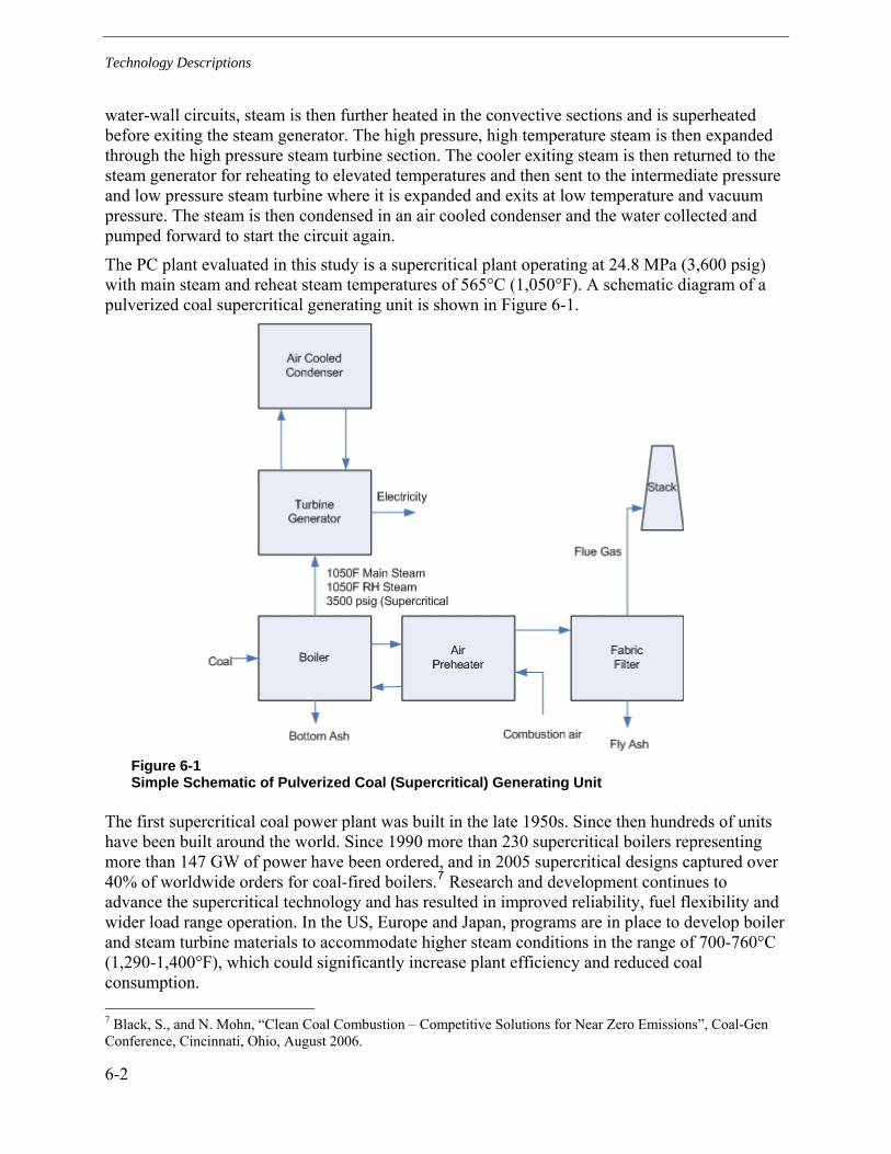
Technology Descriptions
water-wall circuits, steam is then further heated in the convective sections and is superheated before exiting the steam generator. The high pressure, high temperature steam is then expanded through the high pressure steam turbine section. The cooler exiting steam is then returned to the steam generator for reheating to elevated temperatures and then sent to the intermediate pressure and low pressure steam turbine where it is expanded and exits at low temperature and vacuum pressure. The steam is then condensed in an air cooled condenser and the water collected and pumped forward to start the circuit again.
The PC plant evaluated in this study is a supercritical plant operating at 24.8 MPa (3,600 psig) with main steam and reheat steam temperatures of 565°C (1,050°F). A schematic diagram of a pulverized coal supercritical generating unit is shown in Figure 6-1.
Figure 6-1 Simple Schematic of Pulverized Coal (Supercritical) Generating Unit
The first supercritical coal power plant was built in the late 1950s. Since then hundreds of units have been built around the world. Since 1990 more than 230 supercritical boilers representing more than 147 GW of power have been ordered, and in 2005 supercritical designs captured over 40% of worldwide orders for coal-fired boilers.7 Research and development continues to advance the supercritical technology and has resulted in improved reliability, fuel flexibility and wider load range operation. In the US, Europe and Japan, programs are in place to develop boiler and steam turbine materials to accommodate higher steam conditions in the range of 700-760°C (1,290-1,400°F), which could significantly increase plant efficiency and reduced coal consumption. 7 Black, S., and N. Mohn, “Clean Coal Combustion – Competitive Solutions for Near Zero Emissions”, Coal-Gen Conference, Cincinnati, Ohio, August 2006.
6-2

Technology Descriptions
Because of regulations in the US, Europe and Japan, environmental controls for PC plants are progressing to near-zero emissions for SO2, NOX, particulate (including condensables), mercury, and several other hazardous air pollutants such as lead and arsenic. It is becoming more certain that in a few years time, emissions of CO2 will also have to be reduced. However, per the design basis for this study, only flue gas desulfurization (FGD) units are considered for environmental controls on top of pulse jet fabric filters for particulate control.
A limestone forced oxidation (LSFO) wet scrubber is the most widely used FGD system and is the system utilized in this study. The LSFO system uses a variety of gas-liquid contacting devices that have the capability to remove more than 95% of the inlet SO2 and produce a disposable or wallboard-grade gypsum byproduct. This gypsum is able to be marketed in the US, though market analysis should be performed to properly assess the potential for a market for FGD-produced gypsum in South Africa.
The removal of particulate matter, or ash, is accomplished through use of fabric filters housed in structures referred to as baghouses that are located downstream of the air preheaters. Fabric filters are porous cloth media that collect particulate as dust cakes on their surface. Pressure losses are incurred through the baghouse and increase as the particulate collects on the filter, placing an increased demand on fans. The baghouse is regularly pulsed to remove the particulate from the fabric filter for disposal.
Integrated Gasification Combined Cycle (IGCC)
An integrated gasification combined cycle, or IGCC, is a technology that turns coal into gas - synthesis gas or syngas. The gasification plant then removes impurities from the raw syngas before it is combusted. This results in lower emissions of sulfur dioxide, particulates and mercury.
The plant is called "integrated" because heat recovery in the gasification unit is integrated with the plant's combined cycle. Additionally, the gas turbine compressor provides pressurized air used in the air separation unit that produces oxygen for the gasification process. The syngas produced is used as fuel in a gas turbine which produces electrical power. To improve the overall process efficiency, heat is recovered from both the gasification process and also the gas turbine exhaust in a heat recovery steam generator (HRSG) producing steam. This steam is then used in steam turbines to produce additional electrical power.
A schematic diagram of the IGCC power plant is shown in Figure 6-2. It is the integration of the system components that brings the most important advantage of IGCC plants.
6-3

Technology Descriptions
Figure 6-2 Schematic of an IGCC Power Plant
Major components are contained in two groupings, commonly referred to as the “gasification island” and the “power island.” Typically, the capacity of the gasification system is selected to match the fuel needs of the gas turbine, along with design decisions regarding spare gasification capacity, which may be used to increase plant availability or to allow supplemental firing to increase steam production for the steam turbine or process use.
The gasification island of an IGCC plant may resemble any of a number of different stand-alone gasification plants; gasification islands from different suppliers share many common elements but are also technically distinct in several ways. Elements common to IGCC gasification islands generally include a coal preparation area, a gasification reactor, an air separation unit (ASU), gas cooling and clean up, and a water-shift reactor if CO2 capture is included.
The coal preparation area is where coal is pulverized and dried or slurried as necessary for feed to the specific type of gasification reactor. Additives may be added to adjust flow characteristics. Lime or another source of CaO may be added to optimize ash melting point and flow characteristics.
The gasification reactor receives dry or slurried coal, oxygen or air, and in some cases steam, and converts it to raw fuel gas composed chiefly of carbon monoxide, hydrogen, and methane. The reactor may incorporate one or more vessels and have one or two stages of reaction. Dry-feed
6-4

Technology Descriptions
reactors generally require lock hoppers for feed and for slag discharge. Slurry feed reactors may have a slag discharge hopper.
The ASU provides high purity oxygen when the gasifier is oxygen-blown. High-pressure air for the ASU may be provided from the gas turbine compressor or from a separate compressor. Typically, the nitrogen by-product of the ASU is fed back to the combustor for dilution to reduce NOx formation and increase working gas volume.
Gas cooling generally serves double-duty by preheating boiler feedwater and/or generating part of the steam for the steam turbine, in addition to adjusting temperature as required for acid gas clean-up equipment. Gas clean-up removes solids, sulfur, mercury, and other undesired compounds before the fuel gas goes to the combustor(s). A water-shift reactor and CO2 absorber may be added to enable CO2 separation for sequestration and/or to provide hydrogen-rich syngas for other purposes.
The power island of an IGCC plant uses the same basic components as a combined cycle power plant fired with natural gas or distillate oil. Modifications to these components may be made to suit a specific gasification technology. Three major components form the basis of the combined cycle: the gas turbine, the HRSG, and the steam turbine.
The gas turbine (GT) is at the heart of the combined cycle power plant. A multi-stage, axial-flow compressor draws in ambient air and raises its pressure for delivery to the combustor(s). In IGCC, a portion of this air may be redirected to the gasifier (air-blown gasifier) or to an air separation unit (oxygen-blown gasifier). One or more combustors mix fuel with air and combust it to create a high-pressure, high-temperature gas working fluid.
The working fluid exits the combustor(s) and flows through the multi-stage, axial-flow power turbine, which converts its heat energy and kinetic energy into rotational energy. Temperature and stress limits of blade materials in the power turbine are typically the limiting factor in the advancement of GT design for efficiency and power capacity. GTs firing low-heating value syngas often have higher fuel mass flow and lower flame temperatures than the comparable turbine firing natural gas or distillate. In many cases, despite the lower firing temperature, the higher mass flow allows an increase in GT power rating. Some turbine designs are modified with stronger drive shafts and larger generators to take advantage of this capacity.
Exhaust gas from the power turbine is directed to a heat recovery steam generator. The HRSG typically will produce steam at two or three pressures and may incorporate a reheat loop. For IGCC, the gas cooler(s) in the gasification cycle may augment some of the heat exchange surface in the HRSG and/or take the place of feedwater heaters.
Steam from the HRSG is directed to a multi-stage steam turbine. In a single-shaft combined cycle, the steam turbine and the combustion turbine are installed on a common shaft, driving a single generator. In a dual-shaft combined cycle, the steam turbine is installed separately. In larger plants, it is common to have two or three GT/HRSG trains providing steam for a single large steam turbine. Typically, the power output from the steam turbine is about one-third to half of the output from the GT(s). As with conventional combined cycles, the steam turbine will be designed to match characteristics of the combustion turbine, HRSG, and condenser. The different heat, steam, and water requirements of the gasification system will further influence steam turbine and HRSG design.
6-5

Technology Descriptions
The South African coal used in this study has a high ash content and low heating value compared to US coals often analyzed for gasification and IGCC applications. The major coal gasification processes available for commercial license are mostly entrained flow gasifiers (GE, COP and Shell) that operate in the high temperature slagging region. While these entrained flow gasification processes could run the South African coal, the economics would be very adversely affected by the high ash content and lower grade coal. The slurry fed gasifiers of GE and COP would be particularly affected in this regard since achievable energy content of the slurry would probably be even lower than for the US PRB coal, and it is doubtful that GE or COP would offer their process for this coal.
The dry coal fed entrained gasifiers (Shell and Siemens) could handle South African coal, and its low moisture content would prevent the drying costs from being too large. Fluid bed gasifiers such as KBR Transport could also run South African coal; however, the relatively low volatile matter content and the high ash content suggest that the reactivity may not be very high and that the carbon conversion would likely be considerably lower than has been experienced with the low rank more reactive US coals and lignites. IGCC cost and performance estimates for this study are based on a Shell gasifier as a representative of commercially available gasifiers that could be used for this application.
There is an additional economic challenge for IGCC technology because of the high elevation of the mine-mouth power plant sites. The power output of a gas turbine is markedly affected by elevation since the compressor is a constant volume machine. At an elevation of 1800m, the IGCC net MW would be reduced by about 13% from that at sea level. The syngas required would also be less; however, there would be an increase in cost of electricity because some of the economies of scale would be lost.
Fluidized Bed Combustion (FBC)
In fluidized bed combustion (FBC) plants, coal and limestone are fed into a bed of hot particles suspended in turbulent motion (fluidized) by combustion air, blown in through a series of distribution nozzles. The limestone is calcined to form free lime, a portion of which reacts with SO2 to form calcium sulfate. The bed consists of unburned fuel, limestone, free lime, calcium sulfate and ash. In-situ sulfur capture is most efficient between 825 and 875°C (1,520 and 1,610°F) and the boiler is usually designed to operate in this temperature range. The furnace enclosure is a waterwall construction and a convection pass for heat recovery from the flue gas is included. In this respect, the design is similar to that of a conventional PC boiler. Figure 6-3 shows a schematic of a FBC boiler system. As with a PC plant, the heat from combustion heats water in the walls of the boiler, generating steam that is expanded through a steam turbine to produce electricity. The FBC plant evaluated in this study is a subcritical plant with main steam at 16.5 MPa (2,400 psig) and both main steam and reheat steam at 565°C (1,050°F).
6-6

Technology Descriptions
Figure 6-3 Schematic of a Fluidized Bed Combustion Boiler system
FBC boilers operate at gas velocities high enough to entrain the majority of the bed material between 3.7 to 9.1 m/s (12 to 30 ft/s). Typically, a high-efficiency cyclone at the furnace exit is used to separate the entrained material and recycle it back to the bed. To prevent erosion damage in the lower regions of the furnace there are no in-bed tubes and the water walls are lined with refractory. To achieve the required heat duty, in-furnace heat transfer surface (wing walls, panels etc) is added to the water walls which may require an increased furnace height. Some designs provide the additional heat transfer surface with an external heat exchanger (EHE), where boiler tubes are immersed in a bed of the hot solids captured by the cyclone that are fluidized at a velocity sufficiently low to avoid tube erosion. The cooled solids leaving the EHE are then recycled to the foot of the furnace.
As there are no tubes in the bed, air staging is possible in a FBC, which results in lower NOx emissions. Staging means that the lower portion of the bed is supplied typically with 70 percent of the stoichiometric air required and operates under reducing conditions, which inhibit NOx formation. The remaining air is added approximately one fifth of the way up the reactor, just above where the refractory lining ends. Although NOx is reduced, staging increases the amount of CO formed to levels well above those achieved in PC units.
High combustion efficiency is maintained despite the low operating temperature by the use of recycle to extend the in-bed residence time of the fuel particles. This measure also lowers sorbent
6-7

Technology Descriptions
demand by increasing its percent utilization. An additional advantage of the low combustion temperature is that it prevents or limits the slagging of coal ash, thus greatly reducing the fouling of heat transfer surfaces. Hence, FBCs can handle a wide variety of fuels including those difficult to burn in PC boilers, such as high-ash, slagging/fouling coals, and coal wastes. However, this fuel flexibility is assured only if the boiler is designed for the full range of fuels that are intended for use.
If present as separate particles, crushing high ash coal has provided some challenges to operation of FBC units. Crushing the harder ash to achieve the required size distribution for circulation can result in the coal being too fine with it being elutriated from the bed before burning out. This either reduces combustion efficiency or results in fires in the cyclones. Alternatively crushing the coal to the required size distribution for combustion can result in the ash being too coarse to be elutriated into the cyclones and recirculated back to the furnace. It is believed that this issue is being addressed by use of two-stage crushing in preference to the more commonly used single-stage process.
Nuclear Technologies The current fleet of nuclear power plants is a fairly mature technology representing approximately 20% of the electricity generated in the US and over 16% of the electricity generated in the world. It is well suited for large scale stationary applications as well as naval vessels such as submarines and ships. It is especially attractive to countries with limited access to fossil fuels. The major factors driving interest in nuclear power include projected growth in electricity demand, a desire to reduce greenhouse emissions and move away from reliance on fossil fuels, increasing fossil fuel prices, and energy security.
Compared to other large scale central stations, nuclear plants are typically more expensive to construct but less expensive to operate. High construction costs are mostly due to the safety and security requirements, including both design/construction requirements and the lengthy licensing process. Low operating costs are a result of low fuel costs (on a per kWh basis). Therefore, they can be cost effective when construction costs are kept in check and when the plant is to be operated at high capacity for many years. Due to the low operating costs of nuclear reactors, the electricity generation costs are expected to be more stable than those of coal or natural gas-fired plants. They produce no gaseous emissions, although they do generate nuclear waste that poses its own problems. Therefore, CO2 emissions regulations would also tend to make nuclear power economically favorable.
Nuclear power is generated through a fission chain reaction. The heat produced during fission is transferred via gas or liquid to produce steam. Light water reactors (LWR) use standard water as the heat transfer medium and moderator. The moderator turns fast neutrons into thermal neutrons by reducing the neutron’s velocity. The thermal neutrons are then capable of sustaining the fission chain reaction in neighboring uranium atoms. Less commonly used moderators are heavy water and graphite. Fast neutron reactors do not require a moderator, and they utilize a variety of coolants.
Nuclear fuel typically consists of uranium dioxide enriched to 3-5% (by weight) using the uranium-235 isotope. Natural uranium, mixed oxide (MOX) consisting of both plutonium and enriched uranium oxides, thorium, and actinides are also used as nuclear fuel. Uranium prices
6-8

Technology Descriptions
have been increasing over the last several years due mostly to renewed interest in construction of nuclear power plants and recent mining production problems associated primarily with flooding of mines. However, nuclear fuel prices have stabilized recently and compared to other power plant fuel sources, nuclear fuel cost is quite low and has much less volatility.
Generation I nuclear reactors include plants that were developed in the 1950s and 1960s. These reactors typically used unenriched uranium as the fuel, and graphite as the moderator. There are only two still in commercial operation in the United Kingdom; both are scheduled for closure within the next few years.
Generation II nuclear reactors include light water reactors of two primary types – pressurized water reactors (PWR) and boiling water reactors (BWR). PWRs utilize pressurized water as the coolant, with another cooling loop driving the steam turbine. This design contains the radioactivity within the reactor and the primary cooling loop. BWRs allow the water in the cooling loop to boil, and this steam is then used to drive the steam turbine. These Generation II reactors began to be installed in the 1970s, and comprise the vast majority of reactors in operation today. They generally utilize enriched uranium fuel. The advanced gas-cooled reactor (AGR) utilizes graphite as the moderator and natural uranium for fuel. The CANDU reactor also utilizes natural uranium fuel and uses heavy water as its moderator. These reactors include active safety features.
Generation III and III+ nuclear reactors are being constructed and continue to undergo some development. The first was constructed in Japan and has been operating since 1996. They are known as the advanced reactors, and are similar to the Generation II reactors with notable economic and safety advancements. Most of them employ passive safety features rather than active ones, with controls using gravity or natural convection. These reactors are expected to also have reduced nuclear waste and fuel consumption due to higher fuel burn-up. Anticipated lifetime for these reactors is approximately 60 years.
Additionally, several Generation IV nuclear reactor designs are under various stages of development and are expected to become commercially available in the 2030 timeframe. In addition to higher thermal efficiency, the major feature for these reactors will be their ability to integrate into a closed fuel cycles. That is, the long-lived actinides that are currently being treated as nuclear waste could be used as a fuel in these many of these reactors. This may help to reduce waste and cost, while ensuring the fuel associated with these reactors is more resistant to nuclear proliferation. It is also expected that these reactors will be capable of supporting high temperature hydrogen production, high temperature water desalination, and other high temperature process heat applications
This study focused on two Generation III/III+ reactors: Areva’s evolutionary pressurized reactor (EPR) and Westinghouse’s AP1000.
Areva EPR The Areva evolutionary pressurized reactor is based on the PWR design. The first reactor of this type is currently under construction in Finland, with another underway in France. In addition, there are two EPR’s planned for Taishan, China in the Guangdong province. There is a US version of this design known as the US EPR that is rated at 1,600 MW, which is under review by
6-9

Technology Descriptions
the Nuclear Regulatory Commission for licensure. Areva EPR cost estimates for this study are based on the US EPR design.
The US EPR has 241 fuel assemblies surrounded by a neutron reflector to optimize fuel utilization and protect the pressure vessel from radiation damage. The key features of this advanced PWR are an improvement in economy, safety, and reliability. The US EPR has an optimized core design and higher overall efficiency with savings on uranium consumption which reduces the costs of the entire fuel cycle.
The plant is designed to cost 10% less to operate than most of the conventional nuclear plants in service today. The US EPR has been greatly simplified as compared with existing plants. The plant has 47% fewer valves, 16% fewer pumps, 50% fewer tanks, and 44% fewer heat exchangers than the current PWR design. The plant design also has only those features and materials that have shown superior performance over the last 40 years of nuclear power plant operation, improving both reliability and operation and maintenance costs.
The reactor can use various types of fuel, such as low enriched uranium (i.e. up to 5%) or MOX fuel. The US EPR design also allows for a flexible operating cycle (i.e. 12 to 24 months). Another feature of the US EPR that makes it very reliable is that many maintenance and inspection tasks can be completed while the reactor is operating. This in turn also minimizes downtime and maximizes plant efficiency.
The US EPR has four pressurized water coolant loops. The reactor coolant system (RCS) is composed of the reactor vessel that contains the fuel assemblies, a pressurizer including control systems to maintain system pressure, one reactor coolant pump per loop, one steam generator per loop, associated piping, and related control and protection systems. The RCS is contained within a concrete containment building. The reactor containment building has two cylindrical walls with separate domes. The inner wall is made of pre-stressed concrete, the outer of reinforced concrete, and both walls are 1.3 meters thick, designed to withstand postulated external hazards (e.g. airplane crash).
The reactor building is surrounded by four safeguard buildings and a fuel building. The internal structures and components within the reactor building, fuel building, and two safeguard buildings (including the plant control room) are protected against aircraft hazard and external explosions. The other two safeguard buildings are not protected against aircraft hazard or external explosions; however, they are separated by the reactor building, which restricts damage from these external events to a single safety division.
The US EPR has four 100% separate safety systems and uses the latest digital instrumentation that performs continuous self-checking functions. Each safety system is capable of performing the entire safety function for the reactor. This divisional separation is provided for electrical and mechanical safety systems. With four divisions, one division can be out-of-service for maintenance and one division can fail to operate, while the remaining two divisions are available to perform the necessary safety functions even if one is ineffective due to the initiating event.
In the event of a loss of off-site power, each safeguard division is powered by a separate emergency diesel generator (EDG). In addition to the four safety-related diesels that power various safeguards, two independent diesel generators are available to power essential equipment
6-10

Technology Descriptions
during a postulated station blackout event-loss of off-site AC power with coincident failure of all four EDGs.
Water storage for safety injection is provided by the in-containment refueling water storage tank. Also inside containment, below the reactor pressure vessel (RPV), is a dedicated spreading area for molten core material following a postulated worst-case severe accident.
The fuel pool is located outside the reactor building in a dedicated building to simplify access for fuel handling during plant operation and handling of fuel casks. The fuel building is protected against aircraft hazard and external explosions. Fuel pool cooling is assured by two redundant, safety-related cooling trains. Each train consists of two pumps installed in parallel, a heat exchanger cooled by the component cooling water system, and associated piping and valves. The pipe penetrations to the spent fuel pool are above the required level of water that must be maintained over the spent fuel, while providing the required pump suction head. The pipes that penetrate the pool are equipped with siphon breakers to limit water loss resulting from a leak in the piping system.
Figure 6-4 shows the plant layout of the US EPR and Figure 6-5 shows a simplified flow diagram of the EPR.
6-11

Technology Descriptions
Figure 6-4 Example plant layout of the US EPR (provided by AREVA NP)
Figure 6-5 Simplified process flow diagram for the EPR (provided by AREVA NP)
Westinghouse AP1000
The Westinghouse AP1000 is a 1,200 MWe (1,115 MWe net) advanced PWR reactor developed with passive safety systems. The AP1000 power plant is designed as a single unit with a stand-alone configuration. Westinghouse manufactures the AP1000 units in modules for rail and/or barge shipment upon order, which could allow for constructing many modules in parallel with each AP1000 unit virtually identical. The cost estimates within this study are presented for a single unit with a six year project duration from initial engineering to procurement start-up. The schedule and cost for three units and six units constructed in parallel with a 10 year and 16 year project duration, respectively, is also discussed.
The AP1000 power plant has approximately 87% less control cable, 83% less piping (safety grade), 50% fewer valves, 50% less seismic building volume, and 35% fewer pumps than a similarly sized conventional generation II LWR plant. This decrease not only reduces plant costs but also reduces construction schedules. Construction time is further reduced since the AP1000 power plant utilizes a modularization technique for construction.
6-12

Technology Descriptions
The AP1000 power plant fuel design is based on a design used successfully at plants in the US and Europe, which is the 17x17 fuel assembly design. It can operate with Enriched Uranium Dioxide <4.95% Enrichment. Studies have also shown that the AP1000 power plant can operate with a MOX fuel type. This type of fuel is a blend of plutonium, natural uranium, reprocessed uranium, or depleted uranium. The AP1000 has an 18-month fuel cycle and a 17-day refueling outage duration.
The AP1000 uses reduced-worth control rods (termed "gray" rods) to achieve daily load follow without requiring changes in the soluble boron concentration. The use of gray rods, in conjunction with an automated load follow control strategy, eliminates the need for processing thousands of gallons of water per day to change the soluble boron concentration. As a result, systems are simplified through the elimination of boron processing equipment (such as evaporator, pumps, valves, and piping). With the exception of the neutron absorber materials used, the design of the gray rod assembly is identical to that of a normal control rod assembly. The turbine generator is intended for base load operation but also has load follow capability.
A typical site plan for a single unit AP1000 has a power block complex which consists of five principal building structures; the nuclear island, the turbine building, the annex building, the diesel generator building and the radwaste building. Each of these building structures is constructed on individual base mats. The nuclear island consists of the containment building, the shield building, and the auxiliary building, all of which are constructed on a common base mat. A multi-unit plant would consist of multiple single-unit plants with no shared systems.
The AP1000 power plant design is a two-loop, four-reactor coolant pump plan that uses a reactor vessel, internals and fuel similar to those currently used in Westinghouse reactors. The reactor is water cooled and moderated and utilizes enriched uranium fuel. The reactor coolant pumps are designed as canned-type pumps in order to reduce the probability of leakage and to improve reliability. The reactor coolant system pressure boundary provides a barrier against the release of radioactivity generated within the reactor and is designed to provide a high degree of integrity throughout operation of the plant.
The AP1000 steam turbine consists of a double-flow, high-pressure cylinder and three double-flow, low-pressure cylinders that exhaust to individual condensers. It is a six flow tandem-compound, 1,800 rpm machine (1,500 rpm for 50 HZ applications). The turbine generator is intended for base load operation but also has load follow capability.
Figure 6-6is a simplified process flow diagram for a typical PWR like the AP1000.
6-13

Technology Descriptions
Figure 6-6 Typical process flow diagram for a PWR
The AP1000 is designed to achieve a high safety and performance record. The design is conservatively based on proven PWR technology, but with an emphasis on safety features that rely on natural forces. To achieve a high safety and performance record, safety systems use natural driving forces such as pressurized gas, gravity flow, natural circulation flow, and convection rather than active components (such as pumps, fans or diesel generators), and are designed to function without safety-grade support systems (such as AC power, component cooling water, service water, HVAC). The AP1000 passive safety systems are significantly simpler than typical PWR safety systems since they contain appreciably fewer components, reducing the required tests, inspections, and maintenance. They require no active support systems, and their readiness is easily monitored.
The number and complexity of operator actions required to control the safety systems are also minimized. The approach is to eliminate operator action rather than automate it. A few simple valves align and automatically actuate the passive safety systems. To provide high reliability, these valves are designed to actuate to their safeguards positions upon loss of power or upon receipt of a safeguards actuation signal. They are supported by multiple, reliable power sources to avoid unnecessary actuations.
The AP1000 passive safety-related systems include:
• The passive core cooling system
• The passive containment cooling system
• The main control room emergency habitability system
• Containment isolation
These passive safety systems provide a major enhancement in plant safety and investment protection as compared with conventional plants. They establish and maintain core cooling and
6-14

Technology Descriptions
containment integrity indefinitely, with no operator or AC power support requirements. The passive systems are designed to meet the single-failure criteria, and probabilistic risk assessments are used to verify their reliability. Off-site power has no safety-related function due to the passive safety features incorporated in the AP1000 design. Therefore, redundant off-site power supplies are not required. The design provides a reliable off-site power system that minimizes challenges to the passive safety system.
The passive containment cooling system is shown in Figure 6-7.
Figure 6-7 AP1000 passive containment cooling system (provided by Westinghouse Electric Co., LLC)
Gas Technologies
Combined Cycle Gas Turbine (CCGT)
Combined cycle gas turbine (CCGT) technology provides some of the highest plant efficiencies currently attainable among the various technologies examined in this study. This technology is
6-15

Technology Descriptions
based on generating power by combining gas turbines and steam turbine technologies (Brayton and Rankine cycles). Power is generated first in the gas turbines (Brayton Cycle) by burning fuel and the exhaust heat of the gas turbine is recovered in a heat recovery steam generator (HRSG) which provides steam to the steam turbine for generating additional power (Rankine Cycle). A simple schematic of a CCGT arrangement is shown in Figure 6-8.
Figure 6-8 Simple Schematic of CCGT
A gas turbine (GT) includes an air compressor, a combustor, and an expansion turbine. Gaseous or liquid fuels are burned under pressure in the combustor, producing hot gases that pass through the expansion turbine, driving the air compressor. The shaft of the gas turbine is coupled to an electric generator which is driven by the mechanical energy produced by the gas turbine.
The hot exhaust gas exits the GT at temperatures between 538°C and 593°C (1000°F and 1100°F) and passes through a HRSG where it exchanges heat with water producing steam at two or three pressures and may incorporate a reheat loop. The exhaust gas is cooled down to between 80°C and 135°C (176°F and 275°F) before exiting through the HRSG stack. Depending on the selected gas turbine and its associated exhaust temperatures, the high pressure steam conditions from the HRSG range anywhere between 4.32-17.23 MPa(g) (700-2500 psig) with temperatures of 482-565°C (900-1050°F).
The steam produced in the HRSG is used to drive a steam turbine generator. In larger plants, it is common to have two or three GT/HRSG trains providing steam for a single large steam turbine. Usually about two-thirds of the total power is produced from the gas turbines and one-third from the steam turbine. The steam from the steam turbine is condensed using an air-cooled condenser, and the condensate is returned to the HRSG by condensate pumps.
There are various types and categories of gas turbines available in the market today. These include the earlier designed E or lower class turbine models, the state-of-the-art heavy-duty F, G and H class turbine models, and the aeroderivative gas turbines that are generally used in power, combined heat and power, and industrial applications. These gas turbines are available in given sizes or ratings. Their efficiencies are strongly influenced by several factors such as inlet mass flow, compression ratio and expansion turbine inlet temperature. The earlier design of heavy duty gas turbines had maximum turbine inlet temperatures ranging anywhere between 815-1093°C (1500-2000°F). More recent state-of-the-art heavy-duty gas turbine designs have turbine inlet temperatures that reach over 1315-1371°C (2400-2500°F). These turbines are designed with
6-16

Technology Descriptions
innovative hot gas path materials and coatings, advanced secondary air cooling systems, and enhanced sealing techniques that enable higher compression ratios and turbine inlet temperatures. The advancements made in the newer gas turbines by the manufacturers are generally down-flowed into the earlier models for efficiency and power output improvements.
Combined cycle plants can operate with both conventional and advanced gas turbines. With gas turbines running at higher turbine inlet temperatures that result in higher exhaust temperatures, it is possible to include a reheat stage in the steam turbine. This further increases the efficiency in the bottoming cycle.
The combined cycle gas turbine can be built up from the discrete size gas turbine. The HRSG and steam turbine are sized to the exhaust energy available from the gas turbine. There are various configurations of combined cycles with various numbers of HRSG pressure levels. The best heat rates are obtained in combined cycles in which the steam cycle requirements are matched by maximizing the recoverable energy from the gas turbine exhaust. Therefore, various optimized combined cycles can be constructed from a combination of the basic components. The combined cycle plants can be further characterized by the steam cycle (i.e. reheat or non-reheat), HRSG pressure levels (i.e. single pressure, two-pressure, three-pressure) and the number of turbine generator shafts/arrangement (such as single shaft or multi-shaft).
The combined cycle configuration for the purposes of this report will be a multi-shaft, reheat, three-pressure cycle based on the GE 9FA gas turbine. It will consist of 2-9FA gas turbines, each exhausting into a separate HRSG, and a common steam turbine-generator.
Open Cycle Gas Turbine
An open cycle gas turbine is one in which the working fluid remains gaseous throughout the thermodynamic cycle (Brayton cycle). This thermodynamic cycle consists of an adiabatic compression, isobaric heating, adiabatic expansion, and isobaric cooling. In the expansion turbine section of the GT the energy of the hot gases is converted into work. This conversion actually takes place in two steps. In the nozzle section of the turbine, the hot gases expand and a portion of the thermal energy is converted into kinetic energy. In the subsequent bucket section of the turbine, a portion of the kinetic energy is transferred to the rotating buckets and converted to work.
The gas turbine includes an air compressor, a combustor, and an expansion turbine. Air is compressed and then mixed with gaseous or liquid fuels to be burned under pressure in the combustor, producing hot gases that pass through the expansion turbine. The shaft of the GT is coupled to both the air compressor and an electric generator such that mechanical energy produced by the GT drives the electric generator as well as the air compressor. Some of the work developed by the turbine is used to drive the compressor, and the remainder is available for useful work at the output flange of the gas turbine. Typically, more than 50 percent of the work developed by the turbine sections is used to power the axial flow compressor.
There are various types of gas turbines such as heavy-duty industrial, aeroderivative, and advanced heavy-duty gas turbines. Unit sizes are available in a wide range (from 2 MW and smaller to 330 MW and larger). They also have different shaft arrangements. A single-shaft configuration has one continuous shaft between the compressor and the expansion turbine, such that all compressor and expansion turbine stages operate at the same speed. These units are
6-17

Technology Descriptions
typically used for generator-drive applications where significant speed variation is not required. In a two-shaft configuration, the low-pressure or power turbine rotor is mechanically separated from the high-pressure turbine and compressor rotor. This unique feature allows the power turbine to be operated at a wide range of speeds, and makes two-shaft gas turbines ideally suited for variable-speed applications. All of the work developed by the power turbine is available to drive the load equipment, since the work developed by the high-pressure turbine supplies all the necessary energy to drive the compressor.
The main advantages of open cycle GTs include flexibility in siting, low emission levels with natural gas fuel, low capital cost and short construction time. These advantages make them attractive for peaking duty applications. Peaking duty open cycle plot arrangements can be designed to allow for later conversion to combined cycle through staged development.
The performance of a GT is affected by a number of factors, including ambient temperature, relative humidity, fuel type, inlet pressure drop, outlet pressure drop, and site elevation. Higher ambient temperatures or lower ambient pressures (higher altitudes) result in less dense air while lower ambient temperatures or higher ambient pressures (lower altitudes) result in more dense air. Because a gas turbine operates at a fixed volume, lower air density results in reduced mass flow of intake air through the compressor and turbine. Figure 6-9 shows a typical Open Cycle Compressor Inlet Temperature performance curve. This shows the correction factors for open cycle heavy duty GTs to be applied to generated output, heat rate, exhaust flow and heat consumption based on the inlet air temperature. An open cycle altitude correction curve (Figure 6-10) shows the affect of site elevation on GT output and fuel consumption.
Figure 6-9 Open Cycle Compressor Inlet Temperature Performance Curve
6-18

Technology Descriptions
0.7
0.75
0.8
0.85
0.9
0.95
1
0 0.5 1 1.5 2 2.5
Altitude (Thousand meters)
Cor
rect
ion
Fact
or
Figure 6-10 Open Cycle Altitude Correction Curve
As can be seen, the power output of a GT is very sensitive to ambient temperature. Maximum power typically drops about 0.4% for each degree Fahrenheit increase in ambient temperature. For example, a GT with an output rating of about 160 MW at 15ºC ambient temperature at sea level drops to about 140 MW at 32ºC ambient. The reference site conditions (as per ISO standards) for data presented are 15ºC, 60% relative humidity, and sea level elevation.
The gas turbine evaluated in this study is the GE 9001E heavy duty model with an ISO rating of 126 MW operated in peaking service with an annual capacity factor of 10%. An E class GT was used for this open cycle peaking unit due to its better start/stop characteristics compared to the F class GT that is used for combined cycles.
Renewable Technologies
Wind
In recent years, wind has been the fastest growing form of electricity generation in the world. The World Wind Energy Association reports that installed wind capacity worldwide at the end of 2009 was over 152,000 MW with forecasts of continued large-scale installation. Almost all wind power capacity installed to date is on-shore wind. However, the superior wind resources available off-shore along coastlines has lead to considerable research and development of larger off-shore wind turbines and the construction of a few off-shore wind farms.
6-19

Technology Descriptions
On-Shore Wind
During the past 20 years of development, numerous wind turbine design configurations have been proposed and tested, including vertical- and horizontal-axes, upwind and downwind rotors, two or three blades, direct and gearbox-drive train, and fixed-speed, two-speed, and variable-speed generators. Today, the most common wind turbine configuration is the three-blade, upwind, horizontal-axis design with a three-stage gearbox, variable-speed generator and power electronics to generate 50 or 60 Hz power.
The primary components of an on-shore wind turbine include the tower and foundation, the rotor, the nacelle and drive train, rotor pitch and yaw systems, power electronics, and electrical controls, all of which are described in more detail below. Figure 6-11 shows a typical wind turbine.
(Source: US Department of Energy. Energy Information Administration. “Forces Behind Wind Power”. Renewable Energy 2000: Issues and Trends. DOE/EIA-0628. February 2001.)
Figure 6-11 Wind Turbine Front and Side View
The tower is the base that holds the nacelle and the rotor. Typically, turbine towers are constructed from steel. To support the tower, the rotor, and the nacelle, and the dynamic structural loads created by the rotating turbine, a large steel-reinforced concrete foundation designed for the site and soil conditions is typically required.
For large-scale electricity production, multiple wind turbines are typically arranged in single or multiple rows, which are oriented to maximize generation when the wind is from the prevailing
6-20

Technology Descriptions
direction. The wind turbines must be arranged to minimize the impact of wake turbulence on other downwind turbines. To do this, they are often separated by five to 15 rotor diameters downwind and three to five rotor diameters in the direction perpendicular to the wind. Becausindividual wind turbines require a minimal area for the foundation, only 5-10% of the total lcovered by the wind farm is used for the turbines and the remaining land area is available for crop production, grazing land for livestock, or other uses.
At the top of the tower, the rotor blades capture the wind and transfer its power to the rotor huwhich is attached to the low-speed drive shaft. In modern w
e and
b, ind turbines, the pitch of the rotor
ng towards carbon composite blades, which have a much higher length e
enerators, and most use a three-stage
ture
m, rbine is optimally
he wind is below the cut-in speed, the energy in the wind is
rs, wind turbines start up
blades is controlled by individual mechanisms that rotate the blade about its long axis to control the wind load on the turbine in high winds. The blade pitch is controlled to maximize energy production as wind speed varies. The rotor also helps to maintain a constant power output and limit drivetrain overload.
The rotor blades are conventionally fabricated from fiberglass composites. However, the wind industry seems to be movito weight ratio, allowing longer blades to be used as rated capacity increases without making thdynamic loads at the top of the tower proportionately bigger. The rotor blades are attached to the hub, which is typically made from cast iron or steel.
As the rotor blades capture the wind, they rotate the hub and the low-speed shaft of the turbine. Some turbine designs use direct-drive multiple-pole ggearbox to increase the rotation speed and drive the generator to produce electricity. Contrary totypical electrical generators, the rotor, gearbox, and generator are designed to efficiently capwind energy at both low and high wind speeds. Efficiency is less important at higher wind speeds above the rated wind speed, where the blade pitch is adjusted to spill some of the wind in order to maintain the rated power. The nacelle serves as the housing for the gearbox and theelectrical generator and is typically fabricated using fiberglass composites.
The electronic controller monitors the wind turbine’s condition. It controls the yaw mechaniswhich uses an electric motor to rotate the hub and rotor blades so that the tufacing into the wind. It also starts and stops the turbine based on wind speed and shuts down the turbine if there is a malfunction.
Wind turbines are designed to operate within a wind speed window, which is bound by a “cut-in”speed and a “cut-out” speed. When ttoo low to utilize. When the wind reaches the turbine’s cut-in speed, the turbine begins to operate and produce electricity. As the wind speed increases, the power output of the turbine increases until it reaches its rated power. After this, the blade pitch is controlled to maintain the rated power output, even as the wind speed increases, until the wind reaches its cut-out speed. At the cut-out speed, the turbine is shut down to prevent mechanical damage.
Wind plants typically are operated unattended and are monitored and controlled by a supervisorycontrol and data acquisition (SCADA) system. Using onboard computewhen the wind reaches its cut-in speed and shut down when the wind exceeds its cut-out speed or drops back below the cut-in speed. The system is also designed to shut down the turbine if there are any mechanical or electrical failures detected, and maintenance crews will be notified.
6-21

Technology Descriptions
Off-Shore Wind
Some countries have begun to investigate placing wind farms off-shore. The primary difference between offshore and onshore wind turbines is the size and foundation requirements. Due to the high cost of offshore wind turbine foundations and undersea electric cables, offshore wind turbines are typically larger than their onshore counterparts in order to take advantage of economies of scale. In addition to the difference in size, offshore wind turbines have been modified in a number of ways to withstand the corrosive marine environment, such as implementation of a fully-sealed or positive-pressure nacelle to prevent corrosive saline air from coming in contact with critical electrical components, structural upgrades to the tower to withstand wave loading, and enhanced condition monitoring and controls to minimize service trips.
Currently, commercial offshore wind farms are installed in water depths of up to 30 m with foundations fixed to the seabed. The most common foundation type for shallow depths is the steel monopole foundation, which is drilled or driven 25 to 30 m into the seabed. Other types of fixed foundations include steel or concrete gravity bases, which rest on top of the seabed and rely on the weight of the structure to provide stability. Bucket foundations are large-diameter hollow steel structures that are partially driven into the subsea structure by suction and filled with soil and rock to stabilize the foundation. Future developments in offshore wind turbine foundation technology include fixed turbine foundations for transitional depths of 30 m to 60 m and floating turbine foundations for deepwater sites of 60 m to 200 m.
Currently, offshore wind farms are installed at distances from shore ranging from 0.8 km to 20 km. Undersea cables connect the wind turbines within a project to an offshore substation and from the substation to the mainland. Most offshore wind farms utilize high voltage AC transmission lines to transmit power from the offshore substation to the mainland. High voltage DC transmission is a new technology that experiences lower electrical line losses than high voltage AC; however, rectifier and inverter losses are introduced when converting from AC to DC at the offshore substation and from DC back to AC at the onshore grid connection point. The lower line losses are expected to outweigh the additional electrical conversion losses and cost differential only for projects located a significant distance from shore.
This study focused on cost and performance data for on-shore wind.
Solar Thermal
Solar thermal technologies use sunlight to heat a medium and then use the medium to drive a power generation system. Using mirrors, the sun’s energy can be concentrated up to 1,000 times. The concentrated sunlight is then focused onto a receiver containing a gas or liquid that is heated to high temperatures and used to generate steam to drive a power generation system.
The technologies described below are based on the concept of concentrating direct normal irradiation or insolation (DNI) to produce steam used in electricity generating steam turbine cycles. In these technologies the solar power generating systems use glass mirrors that continuously track the position of the sun while absorbing its solar radiation energy. The absorbed solar energy can be harnessed and transferred in two ways: indirectly or directly. The indirect method uses a heat transfer fluid (HTF) which absorbs solar radiation energy and transfers the heat to water via a series of solar steam generator heat exchangers, thus indirectly
6-22

Technology Descriptions
producing steam. The direct method eliminates the HTF step by circulating water directly through the concentrated solar radiation path, thus directly producing steam. Both solar thermal technologies investigated in this study use the indirect method with either a synthetic oil HTF (parabolic trough) or a molten salt HTF (central receiver).
Parabolic Trough
Trough technology uses single-axis tracking, parabolic trough-shaped reflectors to concentrate DNI onto a vacuum absorber pipe or heat collection element (HCE) located at the focal line of the parabolic surface (Figure 6-12). The solar field consists of several hundred to several thousand parabolic trough solar collectors, known as solar collector assemblies (SCAs). Rows of SCAs are aligned on a north-south axis, allowing the single-axis troughs to track the sun from east to west during the day (Figure 6-13). A high temperature heat transfer fluid such as synthetic oil absorbs the thermal energy as it flows through the HCE. Heat collected in the solar field is transported to a series of shell-and-tube heat exchangers – collectively termed a solar steam generator (SSG). The superheated steam generated in the SSG (~370ºC) then expands through a conventional steam turbine to generate electricity.
Parabolic trough systems can be coupled with thermal energy storage (TES) to enhance the dispatchability of the power plant. The current viable TES technology is the indirect molten salt two-tank system. These systems consist of a “cold” tank and a “hot” tank to hold the molten salt and a heat exchanger. During peak hours of solar insolation, some of the heat collected from the solar field in the synthetic oil HTF passes through the heat exchanger of the storage system, transferring heat to molten salt passing from the cold tank to the hot tank. The heated salt is then stored in the hot tank until additional thermal energy is required for the steam cycle. At this time, the hot salt passes back through the heat exchanger, this time heating the synthetic oil HTF, and returns to the cold tank. The heated HTF can then enter the SSG to generate steam for the steam turbine of the power cycle.
Storage rating is a design based on the amount of heat to run the turbine at full output for a specified length of time, for example 125 MW for 3 hours. This specification sizes the storage tanks, piping, pumps, etc. The actual performance of the storage system is based on many parameters including, but not necessarily limited to, the solar multiple used for sizing the field, the operating scheme, the available solar energy, ambient temperatures, etc. The largest factor is the solar multiple, which is the ratio of the solar energy collected at the design point DNI to the amount of solar energy required to generate the rated turbine gross power, and dictates the total amount of heat that can be created by the solar field at any given DNI value. Choosing a solar multiple is a trade off between capital expense and incremental MWh generated. There are times when there will be insufficient energy to charge the storage and run the turbine at full load. There will be other times when parts of the solar field will need to be defocused due to too much heat being available. The concept of solar multiple has been studied extensively, and the solar multiples represented in this study’s designs attempt to strike the best balance between capital expenditure and incremental energy production. Appendix B shows the operating profiles for plants with different amounts of storage for both a summer day and a winter day.
Some important site requirements for a parabolic trough system include having a land slope between 1% and 3% to minimize the trough tilt angle, and a large square to rectangular-shaped land area allowing for north-south SCA row arrangement.
6-23

Technology Descriptions
Figure 6-12 Parabolic Trough
Figure 6-13 Parabolic Trough North-South Axis View
Central Receiver
A central receiver uses two-axis sun-tracking mirrors called heliostats to redirect DNI to a receiver at the top of a tower (Figure 6-14 and Figure 6-15). Molten nitrate salt HTF at 287ºC is pumped out of the “cold” tank, through the receiver, and into the “hot” tank at 565ºC. The “hot” tank delivers the molten salt to the SSG where superheated steam is produced and expanded through a conventional steam turbine producing electricity. Currently, molten nitrate salt has been used as the common HTF because of its superior heat transfer and energy storage capabilities.
6-24

Technology Descriptions
Figure 6-14 Picture of Central Receiver Plant
Figure 6-15 Heliostat to Receiver Sun Path
The ability of molten salt HTF to be heated to 565ºC and generate steam at 538ºC results in relatively higher cycle efficiencies than achievable with the lower temperature steam of the typical synthetic oil HTF parabolic trough plant. The elimination of oil also reduces environmental risks due to leaks and reduces consumable costs because salt is typically significantly cheaper than synthetic oil. However, molten salt has a relatively high freezing point at 221ºC. To maintain salt in the liquid state a significant electrical freeze protection system must be employed. Another disadvantage of this technology is that each mirror must have its own dual-axis tracking control; as a result, tower plants also have larger parasitic loads associated with mirror tracking relative to parabolic trough systems.
6-25

Technology Descriptions
Unlike the synthetic oil HTF parabolic trough system, power tower technology using molten salt allows for direct thermal energy storage, where the HTF is the same fluid as the storage media, allowing for substantial cost reduction of the TES system compared to an indirect TES system because oil to salt heat exchangers are eliminated. Figure 6-16 shows a schematic diagram of the primary flow paths in a molten-salt solar central receiver plant with an integrated two-tank thermal energy storage system.
Figure 6-16 Schematic of Molten-Salt Power Tower System
Typically, central receiver designs have a fixed number of heliostats (solar field size) and a fixed tower height; with the alternating plant design variables being the steam turbine/power block and storage capacities. More specifically, with a larger turbine the plant output is higher at peak solar insolation periods, but less energy is available for storage, whereas a smaller turbine allows for more stored energy, and thus a higher capacity factor, but less peak output to the grid. The optimum balance is highly dependent upon the planned dispatch profile.
Some important site requirements include having a level land area; however the requirements are less stringent than with the trough design, in principle, because of the two-axis mirror tracking. Having a continuous parcel of land able to accommodate an ovular-shaped footprint is also a valuable feature. The footprint of tower systems is relatively larger than a trough based plant.
Solar Photovoltaic Solar photovoltaics (PV) is rapidly becoming a viable utility scale renewable technology option. This technology converts sunlight into electrical power and has been through various levels of commercialization since its development in the 1950s. One of the first applications of solar PV technology was to power remote equipment such as satellites, buoys and telecommunication equipment in combination with batteries to maintain a backup of energy. As costs have decreased and government incentives and mandates have proliferated, applications now span grid-connected homes, buildings and large ground mounted systems.
6-26

Technology Descriptions
The market for solar photovoltaics is growing rapidly. By the end of 2008, the installed global PV capacity was 15,200 MWp, of which 1,100 MWp was installed in the US. The solar PV industry is emerging from its infancy and is quickly growing with mass manufacturing of PV equipment and the commercialization of new technologies. The growth rate of solar capacity has been well above 25% per year over the past few years. In the United States, there has been an increasing focus on utility scale projects, with over 3,000 MWp of utility-scale projects in advanced development.
PV technologies convert sunlight directly into electricity using semiconductor materials that produce electric currents when exposed to light. Semiconductor materials used for PV cells are typically silicon doped with other elements that have either one more or one less valence electrons to alter the conductivity of the silicon. For example, if the silicon is doped with an element having one more valence electron, such as phosphorus, then the resulting material will have an extra electron available for conduction. This material is called an n-type semiconductor. Conversely, when the silicon is doped with an element having one less valence electron, such as boron, then the p-type semiconductor that is produced has an electron vacancy, or hole. When adjacent layers of n-type and p-type materials are illuminated, a voltage develops between them, which can cause a DC electric current to flow in an external circuit.
One characteristic of solar PV that sets it apart from other renewable technologies is its modular nature, which makes it applicable to small distributed systems as well as large utility-scale power plants. The building block of a solar PV system is the PV module, illustrated in Figure 6-17. The solar module consists of multiple solar cells connected in series, and it generates the electrical energy in the form direct current power. Modules are connected in series to form a string in order to increase the voltage of the system. Higher system voltage results in reduced resistance losses across DC collection system wiring distances.
The multiple strings of a PV system are connected in parallel at a combiner box and fed to an inverter, a power electronics device that converts the DC power into AC power. Utility scale systems make use of multiple inverters; for example, a 10-MW plant could have twenty 500-kW inverters. Depending on the technology, the land area required for a 10-MWp power plant varies between 40 and 80 acres or more. Therefore, the distance between the inverters and the point of interconnection to the grid can be significant. To increase the distribution efficiency of the electrical AC energy generated by the inverters in a utility scale system, it is typical to step up the voltage after the inverter to the maximum distribution voltage possible before connecting to a substation for transmission over power lines.
6-27

Technology Descriptions
Figure 6-17 Conceptual Overview of Solar PV System
The nominal power rating of flat plate modules is based on the power output under Standard Test Conditions (STC). STC defines an input energy density of 1,000 W/m2 and a cell temperature of 25° C. The STC rating test is conducted indoors using a solar light simulator that flashes a pulse of controlled and calibrated light over the module. The STC conditions rarely occur in real applications, but the test is relatively easy to replicate and has become the standard to report the nominal power of modules. In solar PV terminology, the power rating is reported as Watt Peak (Wp), to reflect the DC power output of the module under the ideal STC conditions. Two modules with the same power rating may operate with different conversion efficiencies and, therefore, the less efficient module will require a larger active surface area to achieve the same power rating as the more efficient module. The efficiency of the solar PV modules varies from technology to technology. The efficiency of the module has an impact on the land area and balance of system component requirements for a given rated project power. As the efficiency of the modules increases, there is a corresponding decrease in the amount of land area and components such as mounting structures and wiring that are required for a given power generation capacity.
Three array configurations are used for PV systems: fixed-tilt arrays that are stationary and are either mounted flat or oriented to tilt towards the equator for maximum sun exposure, single-axis tracking that tracks the sun’s movement from east to west, and two-axis tracking that tracks the sun to remain perpendicularly oriented to the sun’s rays. There are also three main types of PV technology: flat plate crystalline silicon, thin film, and concentrated PV (CPV). This study focused on fixed-tilt thin-film PV systems and two-axis tracking CPV for commercial- and utility-scale systems.
6-28

Technology Descriptions
Thin-Film
There are two predominant types of flat plate solar PV technologies on the market: crystalline silicon and thin film. Crystalline silicon (c-Si) cells are the most widely used technology to date and is what one traditionally pictures when envisioning a solar panel. However, thin-film modules are being commercialized and are challenging the dominance of crystalline silicon in the PV market. One of the main drivers behind the cost competitiveness of the thin films is the simpler manufacturing process, reduced use of semiconductor materials, and lower manufacturing energy requirements in comparison with crystalline silicon cells.
The manufacturing process for thin film modules typically consists of depositing thin layers of semiconductors on a sheet of glass. Thin film solar cells are made from layers of semiconductor materials only a few micrometers thick; hence the term “thin film”. This process eliminates the ingot growth and wafer sawing steps that are characteristic of crystalline silicon, activities with high energy demand and high semiconductor material waste. A streamlined manufacturing process and a drastic reduction in semiconductor raw material give thin film technologies a cost edge.
Amorphous silicon (a-Si) is the most mature thin film technology, with the longest operating history within the thin films. The first thin film cell was amorphous silicon on a crystalline silicon substrate produced by Sanyo in 1975. Since then, the technology has evolved extensively. The first configuration of amorphous silicon was a single junction cell, which yielded low efficiencies. Double junction and triple junction amorphous silicon followed in efforts to increase conversion efficiency. One approach to increase the conversion efficiency of amorphous silicon modules is to use a tandem junction: the top junction is made of amorphous silicon and the bottom one contains a layer of microcrystalline silicon (μc-Si). This “micromorph tandem” has the potential to significantly expand amorphous silicon’s market share because of higher efficiencies compared to single-junction amorphous silicon and lower manufacturing costs compared to crystalline silicon.
Cadmium telluride (CdTe) is another well developed technology that is competing for and expanding the thin-film market share based on its efficiency and competitive cost. One of the major advantages of CdTe is the relatively simple manufacturing process compared to other thinfilm technologies, which translates into lower equipment capital costs and subsequently lower module costs. The two largest drawbacks to this technology are the toxicity of cadmium and the rarity of tellurium. Elemental cadmium is a well known toxic substance, but it is not known to be toxic in a stable compound form, such as in CdTe. Tellurium is one of the rarest stable solid elements in the earth’s crust, and could become a feedstock bottleneck in the future.
Copper indium gallium (di) selenide, also known as CIGS, is a thin-film technology just now entering the market. CIGS has a long track record in the field, but it is only now beginning to be commercialized on a large scale. It promises a higher efficiency than other thin-film technologies. However, the technology has some drawbacks, such as the use of the rare element indium and a relatively complex manufacturing process. Other thin-film technologies currently in development include dye sensitized solar cells, high-efficiency flexible solar cells, and organic solar cells. Development of these technologies could potentially achieve dramatic reductions in cell cost, but likely will achieve efficiencies on the lower end of the range for solar PV cells.
This study focused on amorphous silicon and cadmium telluride thin-film technologies.
6-29

Technology Descriptions
Concentrating PV
CPV systems make use of optical devices (mirror or lenses) to concentrate the incoming sunlight and deliver it to a photovoltaic cell. The increased energy per unit area allows for a reduction in the surface area of the cell to generate the same amount of power that, without concentration, would have required a cell with a larger surface area. In any photovoltaic system, the photovoltaic cell is the most expensive component. Hence, the main motivation for the development of CPV technologies is to reduce the amount of semiconductor material, while providing an increased power per unit area and using significantly less expensive materials. CPV technologies typically make use of high efficiency tandem or multi-junction cells. Common cell alloys are indium gallium phosphide and gallium arsenide on a germanium substrate. Other materials are being investigated.
Many of the companies working on CPV technologies are still relatively small and early in development. There has been a flood of investments both by private and public entities to commercialize CPV technologies and prove their merit on a large scale. There are also a handful of companies developing low concentration linear concentrators. In addition, some companies that focused on making high efficiency cells for space applications are now developing products for terrestrial systems.
This study focused on high concentration CPV utilizing high efficiency multi-junction cells.
Biomass Biomass fuels are produced by living plant and animal matter. The use of these fuels, which are typically considered renewable fuels, provides electricity generators with dispatchable, non-intermittent renewable power due to the fact that, for the most part, biomass fuels can be produced, concentrated, and stored for use when it is economic to do so.
Biomass fuels exhibit certain fundamental differences from other fossil fuels. Typically, biomass fuels are either gathered up or harvested from diffuse sources and concentrated at a given location. Consequently, there are practical limitations on the quantities that can be obtained at any location without experiencing significant cost pressures. This is in distinct contrast to the fossil fuels that are produced in centralized locations—e.g., coal—and distributed to users such as power plants.
Fuels currently used as biomass fuels are, almost exclusively, residues from other processes. They may be wood processing residues such as hog fuel, bark, sawdust, or spent pulping liquor. They may be agricultural and agribusiness residues such as bagasse. They may be methane-rich gases generated from wastewater treatment plants, landfills, or anaerobic digestion of animal manure. Fractions of municipal solid waste—paper, wood waste, food waste, yard waste—are also forms of biomass fuel. These are all commodities that are presently outside the commercial mainstream. In some cases these commodities have both material and energy value. Wood waste markets, for example, can include mulch for urban areas, bedding for livestock and poultry, feedstocks for materials such as particleboard, and feedstocks for niche chemical and related products. As a result, fuel pricing is highly sensitive to locale and the competitive pressures of local and regional economies.
This study focused on forestry residue and municipal solid waste.
6-30
Technology Descriptions
Forestry Residue
The traditional wood-fired boiler used in electricity generation is a stoker boiler. Producing electricity using biomass boilers is a well-proven technology. Stoker grate boilers utilizing biomass were developed in the 1920-30s. The stoker grate technology is well proven in the biomass power generation industry and is commercially available. It is effective in burning solid fuels that contain fuel particles of sufficient size that they must rest on a grate to burn as well as finely sized particles. Solid fuel is introduced into the furnace using pneumatic or mechanical spreaders, which “stokes” (feeds) the furnace. If the stoker feeds fuel into the furnace by flinging it mechanically or pneumatically over the top of the grate, the stoker is referred to as a spreader stoker. The spreader stoker technology allows for the finely sized particles of the fuel to burn in suspension, while the larger solid fuel particles fall on the grate where they burn to completion. Spreader stokers with oscillating, pulsating, or traveling grates have been widely used for biomass power plants because many of the designed systems have the ability to burn a wide variety of solid fuels simultaneously.
Steam conditions in wood-fired boilers are a function of the design capacity of the boiler. For lower-capacity boilers (e.g., 113,400 kg/hr (250,000 lb/h) steam), 4.1 MPa/400°C (600 psig/750°F) conditions are common. For medium-capacity boilers, the steam conditions are often 5.9 MPa/440°C (850 psig/825°F), and higher capacity units typically use 8.6 MPa/510°C (1,250 psig/950°F) and 10 MPa/540°C (1,450 psig/1,000°F) steam conditions. The larger units use more feedwater heaters to improve the thermal efficiency of the unit.
Turbines are selected based on unit capacity and whether the system is designed as a stand-alone power-only plant, or whether it is a cogeneration or combined heat and power (CHP) plant. Steam turbines can be designed with automatic extractions for process steam or as backpressure turbines exhausting process steam at 345 kPa (50 psig), 1035 kPa (150 psig), or other conditions depending upon the plant requirements. Alternatively the turbines can be designed and supplied to exhaust steam at 6.7 to 10.2 kPa (2 to 3 in HgA) if power is the exclusive product.
Air pollution equipment for solid biomass-fired systems includes either fabric filters (FF) or electrostatic precipitators (ESP) for particulate control. To meet NOx emission standards, stoker grate boiler systems typically include staged combustion systems and accurate combustion control. Combustion is carried out at about 40% excess air, where overfire air accounts for about half the total. Typically, three fans provide the necessary combustion control: one for under-grate combustion air, one for overfire air, and one for pneumatic fuel distributors. Modern stoker boilers also include either selective catalytic reduction (SCR) or selective noncatalytic reduction (SNCR) systems to reduce NOx up to a maximum reduction of 50 %. Acid gas scrubbers are not required due to the compositions of typical solid biomass fuels.
Municipal Solid Waste
Unprocessed municipal solid waste (MSW) and refuse-derived fuel (RDF) are used to generate electricity by burning them in a boiler to produce steam and drive a steam-turbine generator. This study focused on mass burn MSW, which does not process the MSW prior to combustion as is done with RDF. It was chosen for this study because it is the predominant technology for recovering energy and generating electricity from MSW. However, both mass burn MSW and RDF are described for informational purposes.
6-31

Technology Descriptions
Unprocessed MSW typically has a lower heating value than RDF; however, the fuel cost is also lower due to the reduced fuel preparation costs. RDF typically consists of pelletized or fluff material that is the byproduct of a resource recovery operation to remove ferrous and nonferrous materials, such as aluminum and steel cans, glass from bottles and other sources, grit, and other materials that are not combustible. The remaining material is then sold as RDF.
MSW is burned directly in a mass burn boiler. RDF is burned in one of several configurations, including:
• Dedicated RDF boilers designed with traveling grate spreader-stokers;
• Cofiring with coal or oil in multi-fuel boilers;
• Dedicated RDF fluidized boiler.
Various qualities of RDF can be produced, depending on the needs of the user or market. A high quality RDF would possess higher heating value and a lower moisture and ash contents. Processed engineered fuel (PEF), for example, is high quality RDF in which toxic and high-ash components have been removed, as well as metals, rock, glass, electronics, sheet rock, plaster, and other high ash non-combustible components. PEF exists as a fluff, while densified PEF (dPEF) is the same product packed as cubes or pellets for easy storage and transportation.
PEF composite fuels can be formulated to substitute for other solid fuels without modification to the combustion system. E-Fuel is an example of a commercial PEF made with a mixture of 70% paper making waste sludge, 25% waste from a low density polyethylene plastic used to line food cartons, and 5% coal fines. This mixture is blended and then pelletized. Other PEF fuels come in the form of briquettes made from coal fines and other waste materials such as wood.
RDF has relatively high concentrations of paper and plastics, both of which have a high calorific value. In comparison with most coals, it also may contain materials that have a relatively high percentage of ash, can be damaging to burners and boilers, and can impact quality of exhaust gases. For example RDF typically contains materials with substantial concentrations of chlorides that may induce a corrosive effect on boiler tubes. The presence of small particles of metal and of glass fines in RDF can present problems in the combustion system. Moreover, the exclusion of these small particles in RDF is difficult.
Ash production resulting from combustion of MSW or RDF can be four to six times that which would be experienced with the combustion of coal. Consequently, when using RDF in cofiring with coal, some provisions must be made for handling the additional burden of ash.
An important pre-requisite for the successful combustion of RDF/PEF in a combustion system, whether fired solely or in combination with another fuel, is the development of the proper fuel specification. The fuel specification should be provided to the RDF supplier by the combustion system supplier. The need for compatibility of the RDF with all the applicable elements of the combustion system cannot be over emphasized. For financial reasons, optimum performance of the combustion process and thermal conversion system is required. Therefore, the properties of the RDF must be carefully evaluated and selected. These requirements apply to dedicated RDF plants and to cofiring with coal.
RDF composites hold strong potential for both reducing emissions from coal fired boilers and reducing fuel costs. In order to realize both potentials, sources of low cost feedstock must be converted into solid fuel that can be used in existing coal boilers without the need for a capital
6-32

Technology Descriptions
intensive boiler retrofit or a high increase in fuel purchase, transportation, handling and storage costs. Gasification and pyrolysis technologies can convert MSW into energy sources. However, these technologies are less proven in operation, even at relatively modest scale.
Landfill Gas
Gases released from the decomposition of municipal solid waste in landfills are also considered a form of biomass. Solid waste landfills are the largest source of human-related methane emissions in the United States. Landfill gas composition is typically 50% methane, 50% carbon dioxide, and small amounts of other organic compounds. Landfill gas is extracted from landfills using a series of wells and a blower/flare (or vacuum) system. This system directs the collected gas to a central point where it can be processed and treated depending upon the ultimate use for the gas. From this point, the gas can be simply flared or used to generate electricity, replace fossil fuels in industrial and manufacturing operations, fuel greenhouse operations, or be upgraded to pipeline quality gas.
Many sites produce electricity by burning landfill gas in internal combustion engines, small combustion turbines, boilers coupled with steam turbines, and microturbines. Other developing technologies that can use landfill gas are Stirling engines, organic Rankine cycle (ORC) engines, and fuel cells. Thermal applications include packaged boilers, dryers, kilns, greenhouses, water heating for aquaculture, etc. In limited instances, landfill gas has also been compressed and converted to a high-energy gas comparable to pipeline quality natural gas, to liquid fuel, or to feedstock for methanol production. Actively collecting the landfill gas and using it for power generation and thermal uses reduces the contribution of methane to greenhouse gas emissions, reduces the potential for buildup of explosive/toxic releases of methane, and offsets a portion of the natural gas recovered from underground deposits. In this study, the landfill gas is combusted in spark ignition reciprocating engines, which is currently the most common technology used for generating electricity from landfill gas.
6-33


7 COAL TECHNOLOGIES PERFORMANCE AND COST
Pulverized Coal
Table 7-1 Pulverized Coal without FGD Cost and Performance Summary
Technology 2x750 MW, No FGD
4x750 MW, No FGD
6x750 MW, No FGD
Rated Capacity, MW gross 1,599 3,197 4,796 Rated Capacity, MW net 1,500 3,000 4,500 Plant Cost Estimates (January 2010) Total Plant Cost, Overnight, ZAR/kW 16,880 16,025 15,470 Lead Times and Project Schedule, years 5 7 9 Single Unit Expense Schedule, % of TPC
per year 10%, 25%, 45%, 20%
10%, 25%, 45%, 20%
10%, 25%, 45%, 20% 2%, 6%,
13%, 17%*, 17%, 16%, 15%, 11%,
3%
Full Project Expense Schedule, % of TPC per year (* indicates commissioning year of first unit)
5%, 18%, 35%, 32%*,
10%
3%, 9%, 20%, 25%*, 22%, 16%,
5%
Fuel Cost Estimates First Year, ZAR/GJ 15 15 15 Expected Escalation (beyond inflation) 0% 0% 0% Fuel Energy Content, HHV, kJ/kg 19,220 19,220 19,220 Operation and Maintenance Cost Estimates Fixed O&M, ZAR/kW-yr 379 360 348 Variable O&M, ZAR/MWh 36.3 36.3 36.3 Availability Estimates Equivalent Availability 91.7 91.7 91.7 Maintenance 4.8 4.8 4.8 Unplanned Outages 3.7 3.7 3.7 Performance Estimates Economic Life, years 30 30 30 Heat Rate, kJ/kWh Average Annual 9,643 9,643 9,643 100% Load 9,611 9,611 9,611 75% Load 9,779 9,779 9,779 50% Load 10,296 10,296 10,296
7-1

Coal Technologies Performance and Cost
25% Load 12,349 12,349 12,349 Plant Load Factor Typical Capacity Factor 85% 85% 85% Maximum of Rated Capacity 100% 100% 100% Minimum of Rated Capacity 25% 25% 25% Water Usage Per Unit of Energy, L/MWh 33.3 33.3 33.3 Sorbent (Limestone) Usage Per Unit of Energy, kg/MWh 0 0 0 Air Emissions, kg/MWh CO2 924.4 924.4 924.4 SOx 8.93 8.93 8.93 NOx 2.26 2.26 2.26 Hg 1.22E-06 1.22E-06 1.22E-06 Particulates 0.12 0.12 0.12 Solid Wastes kg/MWh FGD solids 0 0 0 Fly ash 166.4 166.4 166.4 Bottom ash 3.28 3.28 3.28
Table 7-2 Pulverized Coal with FGD Cost and Performance Summary
Technology 2x750 MW, With FGD
4x750 MW, With FGD
6x750 MW, With FGD
Rated Capacity, MW gross 1,619 3,237 4,856 Rated Capacity, MW net 1,500 3,000 4,500 Plant Cost Estimates (January 2010) Total Plant Cost, Overnight, ZAR/kW 19,655 18,455 17,785 Lead Times and Project Schedule, years 5 7 9 Single Unit Expense Schedule, % of TPC
per year 10%, 25%, 45%, 20%
10%, 25%, 45%, 20%
10%, 25%, 45%, 20% 2%, 6%,
13%, 17%*, 17%, 16%, 15%, 11%,
3%
Full Project Expense Schedule, % of TPC per year (* indicates commissioning year of first unit)
5%, 18%, 35%, 32%*,
10%
3%, 9%, 20%, 25%*, 22%, 16%,
5%
Fuel Cost Estimates First Year, ZAR/GJ 15 15 15 Expected Escalation (beyond inflation) 0% 0% 0% Fuel Energy Content, HHV, kJ/kg 19,220 19,220 19,220 Operation and Maintenance Cost Estimates Fixed O&M, ZAR/kW-yr 502 472 455 Variable O&M, ZAR/MWh 44.4 44.4 44.4 Availability Estimates Equivalent Availability 91.7 91.7 91.7 Maintenance 4.8 4.8 4.8
7-2

Coal Technologies Performance and Cost
Unplanned Outages 3.7 3.7 3.7 Performance Estimates Economic Life, years 30 30 30 Heat Rate, kJ/kWh Average Annual 9,769 9,769 9,769 100% Load 9,727 9,727 9,727 75% Load 9,913 9,913 9,913 50% Load 10,462 10,462 10,462 25% Load 12,716 12,716 12,716 Plant Load Factor Typical Capacity Factor 85% 85% 85% Maximum of Rated Capacity 100% 100% 100% Minimum of Rated Capacity 25% 25% 25% Water Usage Per Unit of Energy, L/MWh 229.1 229.1 229.1 Sorbent (Limestone) Usage Per Unit of Energy, kg/MWh 15.2 15.2 15.2 Air Emissions, kg/MWh CO2 936.2 936.2 936.2 SOx 0.45 0.45 0.45 NOx 2.30 2.30 2.30 Hg 1.27E-06 1.27E-06 1.27E-06 Particulates 0.13 0.13 0.13 Solid Wastes kg/MWh FGD solids 24.1 24.1 24.1 Fly ash 168.5 168.5 168.5 Bottom ash 3.32 3.32 3.32
Plant Cost Estimates
The total overnight cost for a pulverized coal plant ranges from 15,470 ZAR/kW to 16,880 ZAR/kW for the plants without flue gas desulfurization and from 17,785 ZAR/kW to 19,655 ZAR/kW for plants with flue gas desulfurization, depending on the number of units. It is expected that a plant with multiple units would have a cost advantage over a single unit due to some shared support buildings and infrastructure, as well as the possibility of cost negotiations with contractors for larger purchases. The cost of adding and FGD unit can add about 15% to the cost of the plant on a ZAR per kilowatt basis, due to a combination of the cost of the FGD equipment as well as an increased auxiliary load.
A pulverized coal unit would have about a 4 year expense and construction period. Early in the project, costs will include preliminary design, project siting, and permitting. Later in the project, equipment will be procured, delivered, and installed. This will be when the majority of the expenditures take place. The final stage of the project will be the commissioning of the plant. Based on this schedule, the expected expense schedule is 10% in year 1, 25% in year 2, 45% in year 3, and 20% in year 4. For a multi-unit plant, it is expected that the construction and start-up
7-3

Coal Technologies Performance and Cost
of each unit would be staggered by a year, such that the first unit would start after 4 years and a new unit would start-up each subsequent year.
Fuel Cost Estimates
The cost of the South African coal used in this study is estimated to be 15 ZAR/GJ. with an energy content of about 19,220 kJ/kg. The price of the coal is not expected to increase beyond general inflation.
Operation and Maintenance Cost Estimates
The fixed O&M costs for a pulverized coal plant are between 348-379 ZAR/kW-yr for a plant without FGD and between 455-502 ZAR/kW-yr for a plant with FGD, depending on the number of units. For this study, both maintenance labor and material costs are considered to be fixed O&M costs. The variable O&M costs are 36.3 ZAR/MWh for the plant without FGD and 44.4 ZAR/MWh for the plant with FGD. The FGD unit increases O&M costs both due to increased labor needs (fixed O&M) as well as the additional cost of limestone used in the limestone forced oxidation FGD unit (variable O&M).
Availability and Performance Estimates
The pulverized coal plants have an expected equivalent availability of 91.7% and a capacity factor of 85%. The annual heat rate of the plants without an FGD unit is about 9,640 kJ/kWh and the plants with an FGD unit have an annual heat rate of about 9,770 kJ/kWh. The increased heat rate is due to the added auxiliary load of the FGD unit. An economic life of 30 years is assumed for the pulverized coal plants for cost of electricity calculations; however, the operating life of a coal plant can extend well beyond 30 years.
Cost of Electricity
Table 7-3 and Table 7-4 show a representative levelized cost of electricity for the pulverized coal plants. These assume sequential start-up so that AFUDC accumulates only for a single unit and not for the full schedule of the project. A single start-up at the end of the project would result in a significantly higher AFUDC, resulting in a higher capital expense and higher cost of electricity. These are shown for illustrative purposes only and will vary based on financial assumptions.
Table 7-3 Pulverized Coal without FGD Levelized Cost of Electricity
Technology 2x750 MW, No FGD
4x750 MW, No FGD
6x750 MW, No FGD
Rated Capacity, MW net 1,500 3,000 4,500 Fuel Cost (ZAR/MWh) 144.6 144.6 144.6 VOM (ZAR/MWh) 36.3 36.3 36.3
FOM (ZAR/MWh) 50.9 48.3 46.7
Capital (ZAR/MWh) 321.5 305.5 295.0
7-4

Coal Technologies Performance and Cost
LCOE (ZAR/MWh) 553.4 534.7 522.6
Table 7-4 Pulverized Coal with FGD Levelized Cost of Electricity
Technology 2x750 MW, With FGD
4x750 MW, With FGD
6x750 MW, With FGD
Rated Capacity, MW net 1,500 3,000 4,500 Fuel Cost (ZAR/MWh) 146.5 146.5 146.5 VOM (ZAR/MWh) 44.4 44.4 44.4
FOM (ZAR/MWh) 67.5 63.4 61.1
Capital (ZAR/MWh) 373.9 351.4 338.8 LCOE (ZAR/MWh) 632.4 605.7 590.9
Water Usage
Because the steam cycles of these plants are air-cooled, the only water usage for the plant without FGD is for makeup water to the boiler, which is about 33.3 L/MWh. The addition of wet FGD increases water consumption to 229.1 L/MWh. The use of an air-cooled condenser significantly reduces water consumption. However, use of an air-cooled condenser increases the heat rate by almost 4% compared to a wet-cooled plant, requiring that the rest of the plant, such as turbine generators and auxiliaries to be larger to generate the same amount of steam and output the same amount of electricity.
Emissions
Both the air and solid emissions of the pulverized coal plants evaluated in this study are listed in the summary table above. The installation of an FGD unit drastically reduces the SOx emissions of the plant, though it does slightly increase CO2 and ash emissions due to the slight increase in heat rate and, therefore, coal consumption.
Integrated Gasification Combined Cycle
Table 7-5 Integrated Gasification Combined Cycle Cost and Performance Summary
Technology Two 2x2x1 Shell IGCC
Four 2x2x1 Shell IGCC
Six 2x2x1 Shell IGCC
Rated Capacity, MW gross 1,578 3,157 4,735 Rated Capacity, MW net 1,288 2,577 3,865 Plant Cost Estimates (January 2010) Total Plant Cost, Overnight, ZAR/kW 24,670 23,160 22,325 Lead Times and Project Schedule, years 5 7 9 Single Unit Expense Schedule, % of TPC
per year 10%, 25%, 45%, 20%
10%, 25%, 45%, 20%
10%, 25%, 45%, 20%
Full Project Expense Schedule, % of TPC per year (* indicates commissioning year of
5%, 18%, 35%, 32%*,
3%, 9%, 20%, 25%*,
2%, 6%, 13%, 17%*,
7-5

Coal Technologies Performance and Cost
first unit) 10% 22%, 16%, 5%
17%, 16%, 15%, 11%,
3% Fuel Cost Estimates First Year, ZAR/GJ 15 15 15 Expected Escalation (beyond inflation) 0% 0% 0% Fuel Energy Content, kJ/kg 19,220 19,220 19,220 Operation and Maintenance Cost Estimates Fixed O&M, ZAR/kW-yr 830 779 751 Variable O&M, ZAR/MWh 14.4 14.4 14.4 Availability Estimates Equivalent Availability 85.7 85.7 85.7 Maintenance 4.7 4.7 4.7 Unplanned Outages 10.1 10.1 10.1 Performance Estimates Economic Life, years 30 30 30 Heat Rate, kJ/kWh Average Annual 9,758 9,758 9,758 100% Load 9,652 9,652 9,652 75% Load 10,328 10,328 10,328 50% Load* 12,258 12,258 12,258 25% Load -- -- -- Plant Load Factor Typical Capacity Factor 85% 85% 85% Maximum of Rated Capacity 100% 100% 100% Minimum of Rated Capacity 50% 50% 50% Water Usage Per Unit of Energy, L/MWh 256.8 256.8 256.8 Air Emissions, kg/MWh CO2 857.1 857.1 857.1 SOx (as SO2) 0.21 0.21 0.21 NOx (as NO2) 0.01 0.01 0.01 Solid Wastes kg/MWh Fly ash 9.7 9.7 9.7 Bottom ash 79.8 79.8 79.8 * The heat rate penalty could be mitigated by designing for approximately 50% load on the gasification/ASU system and turn off of one gas turbine.
Plant Cost Estimates
The total overnight cost for the IGCC plant evaluated in this study ranges from 22,325 ZAR/kW to 24,670 ZAR/kW, depending on the number of units. It is expected that a plant with multiple
7-6

Coal Technologies Performance and Cost
units would have a cost advantage over a single unit due to some shared support buildings and infrastructure, as well as the possibility of cost negotiations with contractors for larger purchases.
An IGCC unit would have about a 4 year expense and construction period. Early in the project, costs will include preliminary design, project siting, and permitting. Later in the project, equipment will be procured, delivered, and installed. This will be when the majority of the expenditures take place. The final stage of the project will be the commissioning of the plant. Based on this schedule, the expected expense schedule is 10% in year 1, 25% in year 2, 45% in year 3, and 20% in year 4. For a multi-unit plant, it is expected that the construction and start-up of each unit would be staggered by a year, such that the first unit would start after 4 years and a new unit would start-up each subsequent year.
Fuel Cost Estimates
The cost of the South African coal used in this study is estimated to be 15 ZAR/GJ. with an energy content of about 19,220 kJ/kg. The price of the coal is not expected to increase beyond general inflation.
Operation and Maintenance Cost Estimates
The fixed O&M cost for an IGCC plant ranges from 751 ZAR/kW-yr to 830 ZAR/kW-yr. For this study, both maintenance labor and material costs are considered to be fixed O&M costs. The Shell gasifier has a membrane wall, resulting in a maintenance cost that is slightly lower than for refractory-lined gasifiers. The total staffing requirement for an IGCC is slightly more than for an equivalent sized PC plant due to the more complex processing facilities. The variable O&M cost is 14.4 ZAR/MWh. No credit was assumed for sulfur by-product or for the ash, which is recovered as a glassy, non-leachable slag that can be sold for various building material or roadbed uses.
Availability and Performance Estimates
The IGCC plant evaluated in this study has an expected equivalent availability of 85.7%. This is lower than the expected availability of the other fossil technologies evaluated in this study, largely due to the less mature nature of an IGCC plant and an expected unplanned outage rate of over 10%.
Though the boiler-fired coal plants are unaffected by the higher elevation of the mine-mouth location, the output of the IGCC plant at 1800 m is about 13% lower than the same plant at sea-level. This is because the reduced density of the air at higher elevation reduces the mass flow through the gas turbines. However, the effect of altitude on an IGCC plant is less dramatic than that of a natural-gas fired plant due to the available N2 from the air separation unit that can be used to add mass through the turbine. The annual heater rate of the IGCC plant is expected to be about 9,760 kJ/kWh, which is similar to the pulverized coal units evaluated. At decreased loads, the gas turbine operate less efficiently and the heat rate increases more dramatically than the other coal fired units. However, if the plant is designed correctly, this heat rate penalty can be
7-7

Coal Technologies Performance and Cost
mitigated by turning off one gas turbine and operating the other at full load if the plant is reduced to 50% load.
An economic life of 30 years is assumed for the IGCC plants for cost of electricity calculations; however, it is expected that the operating life of an IGCC could extend well beyond 30 years.
Cost of Electricity
Table 7-6 shows a representative levelized cost of electricity for the IGCC plants evaluated in this study. These assume sequential start-up so that AFUDC accumulates only for a single unit and not for the full schedule of the project. A single start-up at the end of the project would result in a significantly higher AFUDC, resulting in a higher capital expense and higher cost of electricity. These are shown for illustrative purposes only and will vary based on financial assumptions.
Table 7-6 IGCC Levelized Cost of Electricity
Technology Two 2x2x1 Shell IGCC
Four 2x2x1 Shell IGCC
Six 2x2x1 Shell IGCC
Rated Capacity, MW net 1,288 2,577 3,865 Fuel Cost (ZAR/MWh) 146.4 146.4 146.4 VOM (ZAR/MWh) 14.4 14.4 14.4
FOM (ZAR/MWh) 111.5 104.7 100.9
Capital (ZAR/MWh) 468.1 439.8 424.0 LCOE (ZAR/MWh) 740.4 705.2 685.6
Water Usage
The IGCC plant requires water for makeup water to the steam cycle as well as water for steam injection into the gasifier to promote the gasification reactions, resulting in a water consumption rate of about 257 L/MWh. The use of an air-cooled condenser significantly reduces the water consumption compared to a wet-cooled plant, though it increases cost and decreases output.
Emissions
Both the air and solid emissions of the IGCC plant evaluated in this study are listed in the summary table above. The gas cleanup process required before sending the syngas to the gas turbine results in very low SOx and NOx emissions without the need for post-combustion clean up.
7-8

Coal Technologies Performance and Cost
Fluidized Bed Combustion
Table 7-7 Fluidized Bed without FGD Cost and Performance Summary
Technology 2x250 MW, No FGD
4x250 MW, No FGD
6x250 MW, No FGD
Rated Capacity, MW gross 532 1,065 1,597 Rated Capacity, MW net 500 1,000 1,500 Plant Cost Estimates (January 2010) Total Plant Cost, Overnight, ZAR/kW 16,400 15,395 14,840 Lead Times and Project Schedule, years 5 7 9 Single Unit Expense Schedule, % of TPC
per year 10%, 25%, 45%, 20%
10%, 25%, 45%, 20%
10%, 25%, 45%, 20% 2%, 6%,
13%, 17%*, 17%, 16%, 15%, 11%,
3%
Full Project Expense Schedule, % of TPC per year (* indicates commissioning year of first unit)
5%, 18%, 35%, 32%*,
10%
3%, 9%, 20%, 25%*, 22%, 16%,
5%
Fuel Cost Estimates First Year, ZAR/GJ 15 15 15 Expected Escalation (beyond inflation) 0% 0% 0% Fuel Energy Content, kJ/kg 19,220 19,220 19,220 Operation and Maintenance Cost Estimates Fixed O&M, ZAR/kW-yr 402 378 364 Variable O&M, ZAR/MWh 69.1 69.1 69.1 Availability Estimates Equivalent Availability 90.4 90.4 90.4 Maintenance 5.7 5.7 5.7 Unplanned Outages 4.1 4.1 4.1 Performance Estimates Economic Life, years 30 30 30 Heat Rate, kJ/kWh Average Annual 10,060 10,060 10,060 100% Load 10,028 10,028 10,028 75% Load 10,202 10,202 10,202 50% Load 10,735 10,735 10,735 25% Load 12,858 12,858 12,858 Plant Load Factor Typical Capacity Factor 85% 85% 85% Maximum of Rated Capacity 100% 100% 100% Minimum of Rated Capacity 25% 25% 25% Water Usage Per Unit of Energy, L/MWh 33.3 33.3 33.3 Sorbent (Limestone) Usage
7-9

Coal Technologies Performance and Cost
Per Unit of Energy, kg/MWh 0 0 0 Air Emissions, kg/MWh CO2 959.5 959.5 959.5 SOx (as SO2) 9.36 9.36 9.36 NOx (as NO2) 0.20 0.20 0.20 Hg 0 0 0 Particulates 0.09 0.09 0.09 Solid Wastes kg/MWh Gypsum 0 0 0 Fly ash 35.1 35.1 35.1 Bottom ash 140.53 140.53 140.53
Table 7-8 Fluidized Bed with FGD Cost and Performance Summary
Technology 2x250 MW, With FGD
4x250 MW, With FGD
6x250 MW, With FGD
Rated Capacity, MW gross 534 1,067 1,601 Rated Capacity, MW net 500 1,000 1,500 Plant Cost Estimates (January 2010) Total Plant Cost, Overnight, ZAR/kW 16,540 15,530 14,965 Lead Times and Project Schedule, years 5 7 9 Single Unit Expense Schedule, % of TPC
per year 10%, 25%, 45%, 20%
10%, 25%, 45%, 20%
10%, 25%, 45%, 20% 2%, 6%,
13%, 17%*, 17%, 16%, 15%, 11%,
3%
Full Project Expense Schedule, % of TPC per year (* indicates commissioning year of first unit)
5%, 18%, 35%, 32%*,
10%
3%, 9%, 20%, 25%*, 22%, 16%,
5%
Fuel Cost Estimates First Year, ZAR/GJ 15 15 15 Expected Escalation (beyond inflation) 0% 0% 0% Fuel Energy Content, kJ/kg 19,220 19,220 19,220 Operation and Maintenance Cost Estimates Fixed O&M, ZAR/kW-yr 404 379 365 Variable O&M, ZAR/MWh 99.1 99.1 99.1 Availability Estimates Equivalent Availability 90.4 90.4 90.4 Maintenance 5.7 5.7 5.7 Unplanned Outages 4.1 4.1 4.1 Performance Estimates Economic Life, years 30 30 30 Heat Rate, kJ/kWh Average Annual 10,081 10,081 10,081 100% Load 10,048 10,048 10,048 75% Load 10,222 10,222 10,222 50% Load 10,756 10,756 10,756
7-10

Coal Technologies Performance and Cost
25% Load 12,884 12,884 12,884 Plant Load Factor Typical Capacity Factor 85% 85% 85% Maximum of Rated Capacity 100% 100% 100% Minimum of Rated Capacity 25% 25% 25% Water Usage Per Unit of Energy, L/MWh 33.3 33.3 33.3 Sorbent (Limestone) Usage Per Unit of Energy, kg/MWh 28.4 28.4 28.4 Air Emissions, kg/MWh CO2 976.9 976.9 976.9 SOx (as SO2) 0.19 0.19 0.19 NOx (as NO2) 0.20 0.20 0.20 Hg 0 0 0 Particulates 0.09 0.09 0.09 Solid Wastes kg/MWh Gypsum 62.9 62.9 62.9 Fly ash 35.1 35.1 35.1 Bottom ash 140.53 140.53 140.53
Plant Cost Estimates
The total overnight cost for the fluidized bed combustion (FBC) plants evaluated in this study ranges from about 14,840 ZAR/kW to 16,400 ZAR/kW for the plant without FGD and from about 14,965 ZAR/kW to 16,540 ZAR/kW for the plant with FGD. Implementing FGD at the plant by adding limestone to the combustion bed increases total plant cost by less than 1%.
The expected expense and construction period for a single FBC unit is about 4 years. Early in the project, costs will include preliminary design, project siting, and permitting. Later in the project, equipment will be procured, delivered, and installed. This will be when the majority of the expenditures take place. The final stage of the project will be the commissioning of the plant. Based on this schedule, the expected expense schedule is 10% in year 1, 25% in year 2, 45% in year 3, and 20% in year 4. For a multi-unit plant, it is expected that the construction and start-up of each unit would be staggered by a year, such that the first unit would start after 4 years and a new unit would start-up each subsequent year.
Fuel Cost Estimates
The cost of the South African coal used in this study is estimated to be 15 ZAR/GJ. with an energy content of about 19,220 kJ/kg. The price of the coal is not expected to increase beyond general inflation.
Operation and Maintenance Cost Estimates
The fixed O&M costs for the FBC plants are about 364 ZAR/kW-yr to 402 ZAR/kW-yr for the plant without FGD and 365 ZAR/kW-yr to 404 ZAR/kW-yr for the plant with FGD. The major O&M cost difference between the plant without FGD and the plant with FGD occurs in the
7-11

Coal Technologies Performance and Cost
variable O&M due to the additional limestone consumption: variable O&M is 69.1 ZAR/MWh for the plant without FGD and 99.1 ZAR/MWh for the plant with FGD. For this study, both maintenance labor and material costs are considered to be fixed O&M costs. Limestone use is less efficient in an FBC plant compared to a pulverized coal unit, resulting in a more dramatic increase in consumable costs for an FBC plant.
Availability and Performance Estimates
The equivalent availability of the FBC plant evaluated in this study is expected to be about 90.4% and a capacity factor of 85%. The heat rate is 10,060 kJ/kWh for the plant without FGD and 10,081 kJ/kWh for the plant with FGD. There is a slight increase in auxiliary load for the plant with FGD due to the handling of more solids with the addition of limestone, but compared to the emission controls on other fossil plants, the addition of FGD to this plant through the inclusion of limestone in the combustion bed does not adversely affect the heat rate. An economic life of 30 years is assumed for the FBC plants for cost of electricity calculations; however, the operating life of a coal plant can extend well beyond 30 years.
Cost of Electricity
Table 7-9 and Table 7-10 show a representative levelized cost of electricity for the FBC plants evaluated in this study. These assume sequential start-up so that AFUDC accumulates only for a single unit and not for the full schedule of the project. A single start-up at the end of the project would result in a significantly higher AFUDC, resulting in a higher capital expense and higher cost of electricity. These are shown for illustrative purposes only and will vary based on financial assumptions.
Table 7-9 Fluidized Bed without FGD Levelized Cost of Electricity
Technology 2x250 MW, No FGD
4x250 MW, No FGD
6x250 MW, No FGD
Rated Capacity, MW net 500 1,000 1,500 Fuel Cost (ZAR/MWh) 150.9 150.9 150.9
VOM (ZAR/MWh) 69.1 69.1 69.1
FOM (ZAR/MWh) 54.0 50.7 48.9
Capital (ZAR/MWh) 313.1 294.3 283.8 LCOE (ZAR/MWh) 587.1 565.0 552.7
Table 7-10 Fluidized Bed with FGD Levelized Cost of Electricity
Technology 2x250 MW, With FGD
4x250 MW, With FGD
6x250 MW, With FGD
Rated Capacity, MW net 500 1,000 1,500 Fuel Cost (ZAR/MWh) 151.2 151.2 151.2 VOM (ZAR/MWh) 99.1 99.1 99.1
FOM (ZAR/MWh) 54.2 50.9 49.1
7-12

Coal Technologies Performance and Cost
Capital (ZAR/MWh) 316.1 297.1 286.6 LCOE (ZAR/MWh) 620.6 598.3 585.9
Water Usage
Because the steam cycles of these FBC plants are air-cooled, the only water usage is for makeup water to the boiler, which is about 33.3 L/MWh. The addition of in-bed desulfurization does not increase water consumption since it is a totally dry process. The use of an air-cooled condenser significantly reduces water consumption; however, it will increase the heat rate and the plant cost compared to a wet-cooled plant.
Emissions
The air and solid emissions of the FBC plants evaluated in this study are shown in the summary table above. The addition of limestone to the combustion bed significantly reduces the SOx emissions from the plant, though some additional CO2 is released from calcination of the limestone in the FGD. A gypsum byproduct is also produced, which could possibly be sold if a gypsum market is available, or could result in an additional disposal cost.
7-13


8 NUCLEAR TECHNOLOGY PERFORMANCE AND COST
Table 8-1 Nuclear Areva EPR Technology Performance and Cost Summary
Technology 1 Unit 3 Units 6 Units Rated Capacity, MW net 1,600 4,800 9,600 Plant Cost Estimates (January 2010) Total Plant Cost, Overnight, ZAR/kW 28,290 27,605 26,575 Lead Times and Project Schedule, years 6 10 16
Single Unit Expense Schedule, % of TPC per year
15%, 15%, 25%, 25%, 10%, 10%
15%, 15%, 25%, 25%, 10%, 10%
15%, 15%, 25%, 25%, 10%, 10%
3%, 3%, 7%, 7%, 8%, 8%*, 8%, 8%, 8%, 8%, 8%, 8%, 6%, 6%, 2%,
2%
Full Project Expense Schedule, % of TPC per year (* indicates commissioning year of first unit)
15%, 15%, 25%, 25%, 10%, 10%*
5%, 5%, 13%, 13%, 17%, 17%*, 12%, 12%,
3%, 3%
Fuel Cost Estimates First Year, ZAR/GJ 6.25 6.25 6.25 Expected Escalation (beyond inflation) 0% 0% 0% Fuel Energy Content, GJ/kg 3,900 3,900 3,900 Operation and Maintenance Cost Estimates O&M, ZAR/MWh 99.6 97.3 95.2 Availability Estimates Equivalent Availability 92-95% 92-95% 92-95% Maintenance N/A N/A N/A Unplanned Outages <2% <2% <2% Performance Estimates Economic Life, years 60 60 60 Heat Rate, kJ/kWh 10,760 10,760 10,760 Water Usage Cooling (once-through sea water), L/MWh 6,000 6,000 6,000 Boiler Makeup, L/MWh Negligible Negligible Negligible
Table 8-2 Nuclear AP1000 Technology Performance and Cost Summary
Technology 1 Unit 3 Units 6 Units Rated Capacity, MW net 1,200 3,600 7,200
8-1

Nuclear Technology Performance and Cost
Plant Cost Estimates (January 2010) Total Plant Cost, Overnight, ZAR/kW 33,250 32,440 31,215 Lead Times and Project Schedule, years 6 10 16
Single Unit Expense Schedule, % of TPC per year
15%, 15%, 25%, 25%, 10%, 10%
15%, 15%, 25%, 25%, 10%, 10%
15%, 15%, 25%, 25%, 10%, 10%
3%, 3%, 7%, 7%, 8%, 8%*, 8%, 8%, 8%, 8%, 8%, 8%, 6%, 6%, 2%,
2%
Full Project Expense Schedule, % of TPC per year (* indicates commissioning year of first unit)
15%, 15%, 25%, 25%, 10%, 10%*
5%, 5%, 13%, 13%, 17%, 17%*, 12%, 12%,
3%, 3%
Fuel Cost Estimates First Year, ZAR/GJ 6.25 6.25 6.25 Expected Escalation (beyond inflation) 0% 0% 0% Fuel Energy Content, GJ/kg 3,900 3,900 3,900 Operation and Maintenance Cost Estimates O&M, ZAR/MWh 124.4 121.1 118.1 Availability Estimates Equivalent Availability 93% 93% 93% Maintenance 2.8-3% 2.8-3% 2.8-3% Unplanned Outages 4% 4% 4% Performance Estimates Economic Life, years 60 60 60 Heat Rate, kJ/kWh 10,250 10,250 10,250 Water Usage Cooling (once-through sea water), L/MWh 6,000 6,000 6,000 Boiler Makeup, L/MWh Negligible Negligible Negligible
Plant Cost Estimates The total overnight cost for the Areva EPR is estimated to be between 26,575 ZAR/kW and 28,290 ZAR/kW and the total overnight cost for the AP1000 is estimated to be between 31,215 ZAR/kW and 33,250 ZAR/kW, depending on the number of units. While the idealized construction period is 4 years for the Areva EPR and 3 years for the AP1000, it is expected that the construction of a single unit would be closer to a six year project duration from initial engineering and procurement to construction and start-up. Because of some long lead times for procurement of equipment, much of the project cost is incurred in the earlier years of the project, with a total expense profile of 15% in year 1, 15% in year 2, 25% in year 3, 25% in year 4, 10% in year 5, and 10% in year 6.
If multiple units are being built, it is possible that the construction period for the full plant can be condensed compared to building multiple units separately. It is expected that construction of multiple units could occur sequentially with construction on each new unit beginning every two years with sequential start-up as well. A cost reduction of 2.5% per unit was assumed for a multi-unit plant.
8-2

Nuclear Technology Performance and Cost
Fuel Cost Estimates
The fuel cycle for Areva EPR is expected to be between 12 and 24 months. For the AP1000, refueling is expected to occur every 18 months with a 17-day fueling outage. The cost of uranium is estimated to be 6.25 ZAR/GJ. Nuclear fuel costs have been decreasing steadily since 1995 and are expected to stabilize if not continue to decrease. The projected stability in nuclear fuel costs is due to the increased enrichment capacity resulting from construction of new facilities, the improved efficiency of fuel enrichment technology employed by the new facilities, and the effect of fuel reprocessing to reuse fuel or fuel components that have already been partially processed.
Currently enrichment facilities exist in South America, Europe and Asia. Two gas centrifuge enrichment plants are currently under construction in the United State and a third centrifuge plant is planned. Each of these new facilities utilizes centrifuge technology, which consumes 5-10 percent of the energy that the gaseous diffusion enrichment process requires. Employment of centrifuge technology by a larger share of total enrichment capacity lowers the average and marginal production cost of nuclear fuel enrichment and will tend to stabilize, if not decrease nuclear fuel costs over time.
Fuel reprocessing is currently being used in Europe and Asia to recover 20 percent to 30 percent more use from a given amount of uranium. The PUREX method is currently utilized to chemically separate plutonium and uranium. The plutonium and uranium can be returned to the input side of the fuel cycle – the uranium to the conversion plant prior to re-enrichment and the plutonium straight to mixed oxide (MOX) fuel fabrication. One attraction of MOX fuel is that it is a way of disposing of surplus weapon-grade plutonium which otherwise would have to be disposed of as nuclear waste. New reprocessing methods and the use of MOX fuel will reduce need for uranium by reusing fuel or fuel components that have already been partially processed.
Yellow cake prices have varied dramatically since 2005. Since its peak spot price in the second quarter of 2007, prices of yellow cake have decreased and stabilized. Over 80% of uranium is sold on contract, using term prices as a base for the contract price. Individual purchases for near-term delivery are made based on the spot price. Yellow cake spot and term prices are expected to converge in forthcoming quarters as a further indication of price stability.
Operation and Maintenance Cost Estimates
It is expected that manpower requirements for modern nuclear plants will be reduced due the reduction in equipment and focus on passive safety features. Furthermore, advances in on-line diagnostic equipment and control room interfaces will reduce maintenance time. O&M costs are estimated to be between 95.2-99.6 ZAR/MWh for the Areva EPR and between 118.1-124.4 ZAR/MWh for the AP1000, which includes both fixed and variable O&M.
8-3

Nuclear Technology Performance and Cost
Availability and Performance Estimates
Availability of nuclear plants has continued to improve over the years as maintenance practices have been refined and on-line diagnostic equipment has developed. Availability of the nuclear plants is expected to be as high as 92 to 95%.
Though operating licenses are currently issued for 40 years in the United States, it is expected that nuclear plants will have an economic life of 60 years or longer, based on the service life of the reactor vessel.
The heat rate of the Areva EPR is estimated to be 10,760 kJ/kWh and the heat rate of the AP1000 is estimated to be 10,250 kJ/kWh. These plants are expected to operate primarily at full load, but are designed to allow for some load follow capability.
Cost of Electricity
Table 8-3 and Table 8-4 show the levelized cost of electricity of the Areva EPR and the AP1000 nuclear plants. These assume sequential start-up so that AFUDC accumulates only for a single unit and not for the full schedule of the project. A single start-up at the end of the project would result in a significantly higher AFUDC, resulting in a higher capital expense and higher cost of electricity. These are shown for illustrative purposes only and will vary based on financial assumptions.
Table 8-3 Nuclear Areva EPR Levelized Cost of Electricity
Technology 1 Unit 3 Units 6 Units Rated Capacity, MW net 1,600 4,800 9,600 Fuel Cost (ZAR/MWh) 67.3 67.3 67.3 VOM + FOM (ZAR/MWh) 99.6 97.3 95.2
included above FOM (ZAR/MWh) Capital (ZAR/MWh) 570.5 556.7 536.0 LCOE (ZAR/MWh) 737.3 721.3 698.5
Table 8-4 Nuclear AP1000 Levelized Cost of Electricity
Technology 1 Unit 3 Units 6 Units Rated Capacity, MW net 1,200 3,600 7,200 Fuel Cost (ZAR/MWh) 64.1 64.1 64.1 VOM + FOM (ZAR/MWh) 124.4 121.1 118.1
included above FOM (ZAR/MWh) Capital (ZAR/MWh) 670.2 653.9 629.3 LCOE (ZAR/MWh) 858.7 839.1 811.5
8-4

Nuclear Technology Performance and Cost
Water Usage
It was assumed that the nuclear plants in this study are cooled using a once-through cooling sea-water condenser. This condenser has a water requirement of about 6,000 L/MWh, but the water is return to the ocean after it has cooled the condenser, and there is no net consumption of water for cooling purposes. The water makeup necessary for the steam cycle is negligible.
8-5


9 GAS TECHNOLOGIES PERFORMANCE AND COST
Table 9-1 Gas Turbine Cost and Performance Summary
Technology Open Cycle
Gas Turbine
Combined Cycle Gas
Turbine Rated Capacity, MW gross 115.9 732.4 Rated Capacity, MW net 114.7 711.3 Plant Cost Estimates (January 2010) Total Plant Cost, Overnight, ZAR/kW 3,955 5,780 Lead Times and Project Schedule, years 2 3
40%, 50%, 10% Expense Schedule, % of TPC per year 90%, 10%
Fuel Cost Estimates First Year, ZAR/GJ 42.1 42.1 Expected Escalation (beyond inflation) See discussion below Fuel Energy Content, MJ/SCM 39.3 39.3 Operation and Maintenance Cost Estimates Fixed O&M, ZAR/kW-yr 70 148 Variable O&M, ZAR/MWh 0.0 0.0 Availability Estimates Equivalent Availability 88.8 88.8 Maintenance 6.9 6.9 Unplanned Outages 4.6 4.6 Performance Estimates Economic Life, years 30 30 Heat Rate, kJ/kWh Average Annual 11,926 7,486 100% Load 10,841 7,269 75% Load 11,622 7,817 50% Load 13,236 7,941 25% Load 18,227 8,388 Plant Load Factor Typical Capacity Factor 10% 50% Maximum of Rated Capacity 100% 100% Minimum of Rated Capacity 20% 20%
9-1

Gas Technologies Performance and Cost
Water Usage Per Unit of Energy, L/MWh 19.8 12.8 Air Emissions, kg/MWh CO2 622 376 SOx (as SO2) 0 0 NOx (as NO2) 0.28 0.29 Hg 0 0 Particulates 0 0
Plant Cost Estimates The total overnight cost for the open cycle gas turbine (OCGT) is 3,955 ZAR/kW and for the combined cycle gas turbine (CCGT) is 5,780 ZAR/kW. The low cost of the open cycle plant is important for its economic viability as a peaking unit – because it operated infrequently, its annual electricity production is low and it, therefore, has fewer megawatt-hours over which to recover capital expenses.
The expected expense and construction period for an OCGT plant is about 2 years. The first year will include the majority of design, equipment procurement, and construction while the second year will involve the commissioning of the plant, leading to an expected expense schedule of 90% in the first year and 10% in the second year. The CCGT has an expected expense and construction period of about 3 years. The first year will involve permitting at the beginning followed by equipment procurement, delivery and installation in the latter part of the year and into the second year, while the final year of the project will involve commissioning of the plant, leading to an expected expense schedule of 40% in year 1, 50% in year 2, and 10% in year 3.
Fuel Cost Estimates The cost of the liquefied natural gas (LNG) used in this report is estimated to be 42.1 ZAR/GJ with a fuel energy content of 39.3 MJ/SCM.
Predicting the future of LNG prices is a full study in itself. A host of factors influence cost comparisons of pipeline transport of natural gas and liquefaction and transport of LNG. These factors include the cost of liquefaction, whether pipelines are onshore or offshore, and the diameter and pressure of the pipelines, which depend on the quality of the resource available to support high rates of extraction. Figure 9-1 shows calculations by one of the top US natural gas consultants. This figure, as well as subsequent examples, shows that – other things being equal – LNG is the choice for very long-distance transport. A second point arising from the chart is the very sharp contrast between all movements of natural gas and the transport of oil. The cost of oil transport is orders of magnitude cheaper than of natural gas, which is the foundation of explaining the essential commonality of global oil prices and regionality of natural gas prices. Depending on pipeline design, LNG would generally be the more economic choice at distances exceeding 1,800-3,500 miles or 3,000-5,700 km.
9-2

Gas Technologies Performance and Cost
Relative Transportation Costs – 2002 Perspective(Gas Delivery Capability in BCM: 11 Bcm = 1.06 Bcf/d)
Source: James T. Jensen, Jensen Associates, JAI-Energy.com, various references including: “Natural Gas – The ProblemChild of Energy Transport and Trade”, Presentation to The Conference on Global Challenges at the Intersection of Trade,Energy and the Environment – hosted by the World Trade Organization, Geneva, October 22, 2009
Liquefaction
Figure 9-1 Relative Transportation Costs – 2002 Perspective
Figure 9-2 and Figure 9-3 show similar comparisons done in later years. Figure 9-2 portrays a rough comparison with no details on either the LNG or pipeline designs. It shows the effects of a drop in both LNG and pipeline costs, with the crossover point favoring LNG at distances exceeding nearly 5,000 km. The triangular areas on chart to the right mark the envelope formed by the earlier circa-2002 calculations and those presented here.
Source: Riaz Ahmed Kamlani, Shell – Shell Gas and Power, February 2006: LNG Growth – Relevance for Port Authorities. Download from www.iaphworldports.org; citing SGSI 2005 and GPM 2004.
Relative Transportation Costs – 2004 Perspective Cost per MMBTU
Pipeline
$00 2000 4000 6000 8000 10000
kilometres
Pipeline/LNG LNG
LNGOffshore Gas Line
Onshore Gas Line
$4Pipeline
$00 2000 4000 6000 8000 10000
kilometres
Pipeline/LNG LNG
LNGOffshore Gas Line
Onshore Gas Line
$4
Comparison (added)
Liquefaction
crossover points
9-3

Gas Technologies Performance and Cost
Figure 9-2 Relative Transportation Costs – 2004 Perspective
Figure 9-3 shows a reference from 2007 showing a flattening of pipeline costs from the previous examples and an increase in LNG costs, resulting in the crossover favoring LNG not occurring for even low-pressure pipelines until approximately 4,400-5,500 km and, in the case of high-pressure pipelines, potentially not occurring until 8,000-10,000 km. While the basic point remains the same, which is that LNG is typically the best choice for long distant transport (and thus, also, flexibility to access alternative supply sources), an updated assessment of uncommitted supplies and liquefaction costs plus shipping economics and prospects may be needed to support any current commercial assessment.
Relative Transportation Costs – 2007 Reference(Source: ENI re. Maghreb pipeline)
Pipeline
$00 2000 4000 6000 8000 10000
kilometres
Pipeline/LNG LNG
Offshore Lines
Onshore Lines$4
Approx. Comparison (added)
Source: “Compressed Natural Gas: Monetizing Stranded Gas” , By Michael J. Economides and Saeid Mokhatabhttp://www.energytribune.com/articles.cfm?aid=643&idli=3 ; Posted on Oct. 18, 2007
LNG
crossover points(left-LP, rt-HP)
Figure 9-3 Relative Transportation Costs – 2007 Perspective
The natural gas and LNG market has seen large fluctuations in recent years, and a seemingly overnight shift from a seller’s market due to extreme shortages in 2008 to a buyer’s market with large amounts of excess supply. This shift happened for a number of reasons.
During most of the last five years and throughout 2008 the global LNG market primarily was a seller’s market. The major factors that contributed to this market condition are as follows:
• Demand Growth: Expectations until about 2008 were for continuing robust world economic growth, which would trigger large demand growth for natural gas across the globe.
• North American Production Decline: A decline in US and Canadian production during the middle of the decade generated an expectation that a massive need for LNG imports would develop in the US.
9-4

Gas Technologies Performance and Cost
• Oil-Gas Competition: In Asia, the existence of competition between oil and gas in several sectors resulted in oil-linked pricing for natural gas, or premium natural gas prices.
• Record Oil Prices: The strong upward trend of oil prices from about $50 per barrel at the beginning of 2007 to almost $150 per barrel in mid-2008 further enhanced the expectations that gas prices would remain at relatively high levels.
• Decline in Supply: The decline in supply from what was then the world’s largest LNG supplier, namely Indonesia, and the invoking of force majeure conditions reinforced the need, particularly in Asia, to move quickly to secure new LNG supplies.
These conditions, particularly in combination, led to a seller’s market that saw constant upward pressure on both long-term and spot LNG prices. However, by the time the world entered calendar year 2009 almost all of these factors underpinning a seller’s market changed and a new set of circumstances appeared, which included the following:
• Surge in Supply: A record level of new LNG supply was introduced to the global LNG market as a number of long lead time projects were completed and came online.
• The Great Recession: Potentially at the top of the list, or at least equal to the surge in supply, was the impact of the current global recession on global economic growth and as a result global gas demand. Not only has the current recession caused an unexpected near-term downturn in global gas demand, but it likely will have a significant impact on the intermediate-term outlook for the growth in consumption for natural gas.
• The Shales: The surge in production in the US from unconventional resources, and in particular the shales, completely reversed the outlook for future LNG demand in North America, which has significant ramifications for the entire global LNG supply and demand balance.
• Constraints for China and India: While both China and India have been very hesitant to enter into high-priced LNG contracts, both were thought to be excellent sinks if LNG prices declined. To date the latter has not been the case. While India has purchased a few low priced spot cargoes of LNG, its appetite is limited because it is in the process of tripling its domestic production, as a result of the development of its huge discoveries in its offshore K-G basin. In the case of China, its capacity to import LNG is constrained, as it only has two terminals in operation, with a third likely to start operations in 2010.
This combination of suppressed demand growth and surging supply has resulted in a buyer’s market with spot LNG prices declining drastically and Asian spot LNG prices in some cases collapsing below those for Europe and North America. The latter has resulted in spot LNG cargoes moving from the Pacific market to the Atlantic market, whereas a year ago spot cargoes traveled in the opposite direction.
However, it is much less clear what the impact of this change will be on the long-term market for LNG. While there has been unprecedented acquiescence on terms by sellers, in general, sellers are still sticking with an oil-price indication for their long-term pricing terms, particularly for the wealthier Asian nations. However, with respect to the emerging LNG demand centers within Asia, namely China and India, they are attempting to break away from the traditional premium oil-linked LNG prices and are pushing for ‘hub-based’ pricing terms. Similarly, some within the European and North American demand centers are focusing on gas prices linked to major
9-5

Gas Technologies Performance and Cost
transparent and highly liquid future markets (e.g., NYMEX). Over time these differences likely will lead to an asymmetry in LNG prices among the major demand centers and even within certain demand centers. The relevance to South Africa is that the Atlantic trade in LNG will be influenced by abundant “cheap” gas in the US, with the US continuing to play a role on the sidelines as a user of last resort for much of the time period in question. The period after 2020, however, may reflect a sharp tightening of the market balance.
Table 9-2 shows estimated natural gas costs in $/MMBtu based on the US Energy Information Administration (EIA) Annual Energy Outlook (AEO) and EPRI’s estimate for LNG for the Atlantic Basin and Table 9-3 shows these costs converted to ZAR/GJ. These cost estimates are shown in the dollar basis for the year they are estimated and do include general inflation.
Table 9-2 Natural Gas and LNG Estimates ($/MMBtu)
EIA AEO 2010
LNG ESTIMATE FOR ATLANTIC
BASIN
2010 6 6
2015 6.25 6.25
2020 6.5 6.50-7.00
2025 7 7.00-7.50
2030 8 Sharp upward trajectory post-2025 per AEO
Table 9-3 Natural Gas and LNG Estimates (ZAR/GJ)
EIA AEO 2010
LNG ESTIMATE FOR ATLANTIC
BASIN
2010 42.1 42.1
2015 43.9 43.9
2020 45.6 45.6-49.1
2025 49.1 49.1-52.6
2030 56.2 Sharp upward trajectory post-2025 per AEO
These estimates reflect a near-term excess supply of LNG and, therefore, continued lower prices. Perhaps by 2025, depletion of gas shales production and depletion elsewhere, CO2 policy-driven demand growth, and/or default generation choices leading to preference toward dispatchable, lower capital cost equipment could start to drive natural gas prices higher.
9-6

Gas Technologies Performance and Cost
Operation and Maintenance Cost Estimates
The fixed O&M cost is about 70 ZAR/kW-yr for the OCGT plant and about 148 ZAR/kW-yr for the CCGT plant. For this study, both maintenance labor and material costs are considered to be fixed. The assumed coastal location of the gas turbine plants could possibly increase these maintenance costs because salty air could be detrimental to the gas turbine life and could affect filtration systems differently from air in a non-coastal location. Because there are no disposal costs associated with these gas turbine plants and consumables are used in a negligible amount, variable O&M for both the OCGT and the CCGT is zero.
Availability and Performance Estimates
The equivalent availability of both gas turbine plants evaluated in this study is expected to be about 88.8% and both are expected to have an economic life of at least 30 years. The annual heat rate of the OCGT is 11,926 kJ/kWh, and the plant become much less efficient when it is run at part-load. The combined cycle plant has a heat rate of 7,486 kJ/kWh. This is the most efficient fossil fuel plant due to its utilization of the waste heat exiting the gas turbine for use in the steam turbine. As a peaking plant, the open cycle gas turbine has an expected capacity factor of 10% while the combined cycle has a capacity factor of 50%.
Cost of Electricity
Table 9-4 shows a representative levelized cost of electricity for the gas turbine plants evaluated in this study. These are shown for illustrative purposes only and will vary based on financial assumptions.
Table 9-4 Gas Turbine Levelized Cost of Electricity
Technology Open Cycle Gas Turbine
Combined Cycle Gas
Turbine Rated Capacity, MW net 114.7 711.3 Fuel Cost (ZAR/MWh) 502.1 315.2 VOM (ZAR/MWh) 0.0 0.0 FOM (ZAR/MWh) 77.5 18.1 Capital (ZAR/MWh) 817.4 126.8 LCOE (ZAR/MWh) 1397.0 460.1
Water Usage
For both plants, water injection is used in the gas turbine for NOx control purposes. In addition, some makeup want will be needed for the steam cycle of the combined cycle plant. However, air-cooling of the combined cycle plant greatly reduces water consumption compared to a wet-cooled plant. The water use in the open cycle plant is 19.8 L/MWh and for the combined cycle is
9-7

Gas Technologies Performance and Cost
12.8 L/MWh. The reduced water usage on a per unit of energy basis for the combined cycle is due to its improved efficiency over the open cycle plant.
Emissions
The air emissions of the gas turbine plants evaluated in this study are shown in the summary table above. Natural gas is a much less carbon intensive fuel than coal, resulting in much lower CO2 emission on a per MWh basis than the coal-fired plants.
9-8

10 RENEWABLE TECHNOLOGIES PERFORMANCE AND COST
Wind
Table 10-1 Wind Technology Performance and Cost Summary
Technology 10 x 2 MW 25 x 2 MW 50 x 2 MW 100 x 2 MWRated Capacity, MW net 20 50 100 200 Plant Cost Estimates (January 2010) Total Plant Cost, Overnight, ZAR/kW 16,930 15,890 15,150 14,445 Lead Times and Project Schedule, years 2-3.5 2.5-4 3-5 3-6
Expense Schedule, % of TPC per year 5%, 5%, 90%
2.5%, 2.5%, 5%, 90%
5%, 5%, 10%, 80%
2.5%, 2.5%, 5%, 15%,
75% Operation and Maintenance Cost Estimates Fixed O&M, ZAR/kW-yr 312 293 279 266 Availability Estimates 94-97% 94-97% 94-97% 94-97% Performance Estimates Economic Life, years 20 20 20 20 Capacity Factor See Table 10-2
Plant Cost Estimates
The total overnight cost for the wind technology ranges from 14,445 ZAR/kW for a 200 MW plant to 16,930 ZAR/kW for a 20 MW plant. It is expected that the total project schedule for a wind farm, including preconstruction siting and lead times as well as construction, would be 2 to 3.5 years for a 20 MW plant, 2.5 to 4 years for a 50 MW plant, 3 to 5 years for a 100 MW plant, and 3 to 6 years for a 200 MW plant. It is expected that most of the costs in the earlier months of the project will be permitting, while the equipment procurement and installation will be in the latter months, leading to a heavier weighting of expenses later in the project. It is expected that the year of commissioning would be around 2013-2016 depending on the plant size.
Operation and Maintenance Cost Estimates
First year O&M costs for wind turbines range from 266 ZAR/kW-yr for a 200 MW plant to 312 ZAR/kW-yr for a 20 MW plant. These costs include both maintenance labor and materials. Due to the lack of consumables or disposal costs for wind farms, variable O&M is zero. O&M costs
10-1

Renewable Technologies Performance and Cost
typically increase during the project life by 1-2% per year as major components wear and require more maintenance. As with capital costs, larger projects typically experience economies of scale with O&M costs.
Availability and Performance Estimates
Wind farms are expected to have an availability in the range of 94-97%. A major factor contributing to this high availability is the fact that maintenance can be performed on a single turbine while the remainder of the plant remains in service. The economic life of a wind turbine is expected to be about 20 years.
The performance of a wind turbine depends primarily on the wind resource available. Table 10-2 shows the capacity factor of a wind turbine for wind classes 3 through 6. While the wind resource map in Figure 3-2 shows the wind speeds across South Africa at 10 meter measurement height, this study assumed a hub height of 80 meters. The 10-m wind speeds are converted to 80-m wind speeds using a power law function of elevation with a 0.14 exponent.
Table 10-2 Wind Turbine Capacity Factors
Wind Class 3 4 5 6 Average Wind Speed (m/s @ 10-meter measurement height) 5.3 5.8 6.2 6.7
Average Wind Speed (m/s @ 80-meter hub height) 7.2 7.8 8.3 9
Net Capacity Factor, % 29.1 33.2 36.6 40.6
Cost of Electricity
Table 10-3 through Table 10-6 show representative levelized costs of electricity of the wind plants at different wind classes. These are shown for illustrative purposes only and will vary based on financial assumptions. It can be seen that higher wind classes result in improved levelized costs of electricity.
Table 10-3 Wind Levelized Cost of Electricity – 10 x 2 MW Farm
Technology Wind Rated Capacity, MW net 20
3 4 5 6 Wind Class 0.0 0.0 0.0 0.0 Fuel Cost (ZAR/MWh) 0.0 0.0 0.0 0.0 VOM (ZAR/MWh)
122.4 107.2 97.3 87.7 FOM (ZAR/MWh) 930.0 815.1 739.4 666.6 Capital (ZAR/MWh)
LCOE (ZAR/MWh) 1052.3 922.4 836.7 754.3
10-2

Renewable Technologies Performance and Cost
Table 10-4 Wind Levelized Cost of Electricity – 25 x 2 MW Farm
Technology Wind Rated Capacity, MW net 50 Wind Class 3 4 5 6 Fuel Cost (ZAR/MWh) 0.0 0.0 0.0 0.0 VOM (ZAR/MWh) 0.0 0.0 0.0 0.0
FOM (ZAR/MWh) 114.9 100.7 91.3 82.3
Capital (ZAR/MWh) 875.3 767.2 695.9 627.3 LCOE (ZAR/MWh) 990.1 867.9 787.2 709.7
Table 10-5 Wind Levelized Cost of Electricity – 50 x 2 MW Farm
Technology Wind Rated Capacity, MW net 100
3 4 5 6 Wind Class 0.0 0.0 0.0 0.0 Fuel Cost (ZAR/MWh) 0.0 0.0 0.0 0.0 VOM (ZAR/MWh)
109.5 96.0 FOM (ZAR/MWh) 87.1 78.5
Capital (ZAR/MWh) 847.4 742.7 673.7 607.3 LCOE (ZAR/MWh) 956.9 838.7 760.8 685.9
Table 10-6 Wind Levelized Cost of Electricity – 100 x 2 MW Farm
Technology Wind Rated Capacity, MW net 200 Wind Class 3 4 5 6 Fuel Cost (ZAR/MWh) 0.0 0.0 0.0 0.0 VOM (ZAR/MWh) 0.0 0.0 0.0 0.0
FOM (ZAR/MWh) 104.4 91.5 83.0 74.9
Capital (ZAR/MWh) 813.3 712.9 646.7 583.0 LCOE (ZAR/MWh) 917.8 804.4 729.7 657.8
Solar Thermal
Table 10-7 Parabolic Trough Cost and Performance Summary
Technology 0 Hours Storage
3 Hours Storage
6 Hours Storage
9 Hours Storage
Rated Capacity, MW net 125 125 125 125 Plant Cost Estimates (January 2010) Total Plant Cost, Overnight, ZAR/kW 27,450 37,425 43,385 50,910 Lead Times and Project Schedule, years 4 4 4 4
Expense Schedule, % of TPC per year 10%, 25%, 45%, 20%
10%, 25%, 45%, 20%
10%, 25%, 45%, 20%
10%, 25%, 45%, 20%
Operation and Maintenance Cost Estimates
10-3

Renewable Technologies Performance and Cost
Fixed O&M, ZAR/kW-yr 424 513 562 635 Availability Estimates 95% 95% 95% 95% Performance Estimates Economic Life, years 30 30 30 30 Solar to Electric Efficiency 13.3% 13.2% 13.5% 13.6% Capacity Factor (in Upington, SA) 25.0% 31.2% 36.3% 43.7% Water Usage Per Unit of Energy, L/MWh 270 250 245 245
Table 10-8 Central Receiver Cost and Performance Summary
3 Hours Storage
6 Hours Storage
9 Hours Storage
12 Hours Storage
14 Hours Storage Technology
Rated Capacity, MW net 125 125 125 100 100 Plant Cost Estimates (January 2010) Total Plant Cost, Overnight, ZAR/kW 26,910 32,190 36,225 39,025 40,200 Lead Times and Project Schedule, years 4 4 4 4 4
10%, 25%, 45%, 20%
10%, 25%, 45%, 20%
10%, 25%, 45%, 20%
10%, 25%, 45%, 20%
10%, 25%, 45%, 20%
Expense Schedule, % of TPC per year
Operation and Maintenance Cost Estimates Fixed O&M, ZAR/kW-yr 489 546 603 660 701 Availability Estimates 92% 92% 92% 92% 92% Performance Estimates Economic Life, years 30 30 30 30 30 Solar to Electric Efficiency 16.2% 15.9% 15.8% N/A N/A Capacity Factor (in Upington, SA) 29.2% 36.7% 41.0% 46.8% 47.6% Water Usage Per Unit of Energy, L/MWh 280 295 315 305 316
Plant Cost Estimates
The total overnight cost for the parabolic trough ranges from 27,450 ZAR/kW for a plant without storage to 50,910 ZAR/kW for a plant with 9 hours of storage. For the central receiver, costs range from 26,910 ZAR/kW for a plant with 3 hours of storage to 36,225 ZAR/kW for a plant with 9 hours of storage. Assuming similar scaling for larger amounts of storage, the 100 MW plants with 12 and 14 hours of storage had a total overnight cost range of 39,025 ZAR/kW to 40,200 ZAR/kW.
It is expected that a parabolic trough or a central receiver plant would have a 4 year expense and construction period. Early in the project, costs will include preliminary design, project siting, and permitting. Later in the project, equipment will be procured, delivered, and installed. This will be when the majority of the expenditures take place. The final stage of the project will be the commissioning of the plant. Based on this schedule, the expected expense schedule is 10% in
10-4

Renewable Technologies Performance and Cost
year 1, 25% in year 2, 45% in year 3, and 20% in year 4. It is expected that the year of commissioning would be around 2014-2015.
Operation and Maintenance Cost Estimates
First year O&M costs for parabolic troughs range from 424 ZAR/kW-yr for a plant without storage to 635 ZAR/kW-yr for a plant with 9 hours of storage. For the central receiver, O&M costs range from 489 ZAR/kW-yr for a plant with 3 hours of storage to 701 ZAR/kW-yr for a plant with 14 hours of storage. These costs include both maintenance labor and materials. Due to the lack of consumables or disposal costs for solar thermal plants, variable O&M is zero. It is expected that O&M holdback will remain relatively constant (in constant dollars) for the life of the plant.
Availability and Performance Estimates
Parabolic troughs are expected to have an availability of up to 95% while central receivers are expected to have an availability of 92% due to their early commercial status. It is expected that as more systems are deployed that the availability of central receiver plants will converge with those of parabolic troughs. Because the solar fields do not operate at night, much of the required maintenance can take place during this down time. Furthermore, due to the modular nature of the collectors and heliostat mirrors, many repairs can take place on a single section of the solar field while the remainder remains in operation. The economic life of a solar thermal plant is expected to be about 30 years.
As the amount of storage included at a solar thermal plant increases, the annual output and capacity factor of the plant increases. The actual output of a solar thermal plant is highly dependent on the solar resource at the site, and the capacity factors presented in this study are for a plant located near Upington, South Africa. For a parabolic trough without storage, the capacity factor is expected to be about 25% while a plant with 9 hours of storage has a capacity factor of 43.7%. In the same manner, a central receiver with only 3 hours of storage has a capacity factor of 29.2% while a plant with 9 hours of storage has a capacity factor of 41%. This increased plant output requires the additional storage equipment and additional mirrors or collectors, resulting in increased plant cost. Therefore, the costs and benefits of storage must be considered to find the optimum design. As a follow-on to the initial evaluation, a 100 MW with 12 and 14 hours of storage was also evaluated. These plants with higher storage amounts had capacity factors of 46.8% and 47.6%, respectively.
Cost of Electricity
Table 10-9 and Table 10-10 show a representative levelized cost of electricity of the parabolic trough and central receiver for a range of storage hours. These are shown for illustrative purposes only and will vary based on financial assumptions. Central receivers are in the pre-commercial to early commercial phase of development, and any early projects, particularly with large amounts of thermal energy storage, will likely have a different financial structure with a higher equity ratio and a higher cost of debt. Rather that speculate what this structure may be like, the same
10-5

Renewable Technologies Performance and Cost
assumptions were used for all solar technologies to illustrate any capital and/or operational advantages of each case. It can be seen that the number of hours of storage can be optimized to find the lowest cost of electricity based on the increased output of the plant due to storage compared to the increased cost of the plant.
Table 10-9 Parabolic Trough Levelized Cost of Electricity
Technology Parabolic Trough 125 Rated Capacity, MW net
Hours of Storage 0 3 6 9 Fuel Cost (ZAR/MWh) 0.0 0.0 0.0 0.0 VOM (ZAR/MWh) 0.0 0.0 0.0 0.0
FOM (ZAR/MWh) 193.3 187.6 176.7 166.0
Capital (ZAR/MWh) 1751.9 1913.4 1907.0 1859.8 LCOE (ZAR/MWh) 1945.2 2101.0 2083.7 2025.8
Table 10-10 Central Receiver Levelized Cost of Electricity
Technology Central Receiver Rated Capacity, MW net 125 100 Hours of Storage 3 6 9 12 14 Fuel Cost (ZAR/MWh) 0.0 0.0 0.0 0.0 0.0 VOM (ZAR/MWh) 0.0 0.0 0.0 0.0 0.0
FOM (ZAR/MWh) 191.1 169.8 167.9 160.9 168.0
Capital (ZAR/MWh) 1472.1 1400.5 1411.3 1331.4 1348.7 LCOE (ZAR/MWh) 1663.2 1570.3 1579.1 1492.3 1516.7
Water Usage
Because the plants in this study were evaluated with air cooled condensers, the primary use of water in these solar thermal plants is due to mirror washing. It is expected that about 115 liters of water is required per meter squared of mirror area per year assuming that mirrors are washed about once a week. A small amount of water will also be needed for power block make-up. Air cooled plants typically save around 90% of the water used in a similar wet-cooled plant.
Photovoltaics
Table 10-11 CdTe PV Cost and Performance Summary
Technology Thin Film Fixed Tilt CdTe Mounting Location Rooftop (0° tilt) Ground (latitudinal tilt) Rated Capacity, MW net 0.25 1 1 10 Plant Cost Estimates (January 2010) Total Plant Cost, Overnight, ZAR/kW 42,020 34,200 36,000 28,055 Lead Times and Project Schedule, years 1 1 2 2
10-6

Renewable Technologies Performance and Cost
Expense Schedule, % of TPC per year 100% 100% 10%, 90% 10%, 90% Operation and Maintenance Cost Estimates Fixed O&M, ZAR/kW-yr 402 402 402 402 Availability Estimates 98% 98% 98% 98% Performance Estimates Economic Life, years 25 25 25 25 Capacity Factor See Table 10-14Water Usage, L/yr 11,270 45,080 45,080 450,800
Table 10-12 Amorphous Silicon PV Cost and Performance Summary
Technology Thin Film Fixed Tilt a-Si Mounting Location Rooftop (0° tilt) Ground (latitudinal tilt) Rated Capacity, MW net 0.25 1 1 10 Plant Cost Estimates (January 2010) Total Plant Cost, Overnight, ZAR/kW 43,400 35,250 37,095 28,910 Lead Times and Project Schedule, years 1 1 2 2 Expense Schedule, % of TPC per year 100% 100% 10%, 90% 10%, 90% Operation and Maintenance Cost Estimates Fixed O&M, ZAR/kW-yr 402 402 402 402 Availability Estimates 98% 98% 98% 98% Performance Estimates Economic Life, years 25 25 25 25 Capacity Factor See Table 10-14Water Usage, L/yr 8,480 33,935 33,935 339,350
Table 10-13 Concentrating PV Cost and Performance Summary
Technology Concentrating PV
Rated Capacity, MW net 10 Plant Cost Estimates (January 2010) Total Plant Cost, Overnight, ZAR/kW 37,225 Lead Times and Project Schedule, years 2 Expense Schedule, % of TPC per year 10%, 90% Operation and Maintenance Cost Estimates Fixed O&M, ZAR/kW-yr 502 Availability Estimates 95% Performance Estimates Economic Life, years 25 Capacity Factor (1st Year) 29.1% Capacity Factor (Average) 26.8%
10-7

Renewable Technologies Performance and Cost
Water Usage, L/ yr 395,890
Plant Cost Estimates
The total overnight cost for CdTd PV systems ranges from 28,055 ZAR/kW for a 10 MW ground mounted plant to 42,020 ZAR/kW for a 250 kW roof mounted system. For amorphous silicon PV, the total overnight cost ranges from 28,910 ZAR/kW for a 10 MW ground mounted plant to 43,400 ZAR/kW for a 250 kW roof mounted system. A 10 MW concentrating PV system is estimated to cost 37,225 ZAR/kW for a dual axis tracking system. It is expected that roof mounted systems can be sited, permitted, and constructed within a year, while ground mounted systems can be completed within 2 years, with about 10% of the costs being incurred in year 1 and 90% in year 2. It is expected that the year of commissioning would be around 2013-2014.
Operation and Maintenance Cost Estimates
First year O&M costs for both CdTe and amorphous silicon thin film fixed tilt PV plants are expected to be 402 ZAR/kW. While ground mounted systems include the cost of the land purchased for the system in their capital costs, roof mounted systems typically include the annual lease cost of the roof space in the fixed O&M. However, these estimates do not include this extra cost. O&M for a two axis tracking CPV plant is expected to be 502 ZAR/kW. These fixed O&M costs include both maintenance labor and materials. Due to the lack of consumables or disposal costs for PV plants, variable O&M is zero.
Availability and Performance Estimates
The fixed tilt PV systems are expected to have an availability of 98%, while the CPV system is expected to have an availability of 95%. As with solar thermal plants, the fact that the plants do not operate at night allows for some of their maintenance to take place during hours of non-operation. Furthermore, their modularity allows for individual modules to be services without shutting down the entire system. The economic life of PV systems is expected to be about 25 years.
The performance of a PV system is highly dependent on the solar resource available. The performance of the flat plate PV systems was evaluated in both Cape Town and Johannesburg, South Africa. The rooftop mounted panels were assumed to be installed without any tilt, while the ground mounted panels were assumed to be installed tilted at latitude, maximizing annual energy output. Experience has shown that photovoltaic modules decrease in output over time due to a number of reasons. Most manufacturers guarantee 80% of the original output at standard conditions after 25 years. This translates into a 0.8% per year energy degradation factor included in the price modeling. Capacity factors were calculated for the first year of operation, as well as the average over the 25 year life of the panels assuming degradation in panel output of 0.8% per year. Table 10-14 shows the capacity factors for both locations and thin film types both for the first year and the average for 25 years.
The performance of the CPV system was evaluated for a site near Upington. The capacity factor was calculated for the first year of operation, as well as the average over the 25 year life of the
10-8

Renewable Technologies Performance and Cost
CPV panels assuming a degradation in panel output of 0.7% per year. This resulted in a first year capacity factor of 29.1% and an average capacity factor of 26.8%.
Table 10-14 Thin Film PV Capacity Factors
Technology CdTe a-Si
Mounting Location Rooftop (0° tilt) Ground (latitudinal tilt) Rooftop (0° tilt) Ground
(latitudinal tilt) Cape Town (1st Year) 18.7% 20.7% 18.7% 20.7% Cape Town (Average) 17.0% 18.8% 17.0% 18.9% Johannesburg (1st Year) 19.4% 21.4% 19.4% 21.4% Johannesburg (Average) 17.6% 19.4% 17.6% 19.4%
Cost of Electricity
Table 10-15 through Table 10-19 show the representative levelized costs of electricity of the PV plants. These are shown for illustrative purposes only and will vary based on financial assumptions. It can be seen that the economy of scale of the larger ground-mounted systems result in lower costs of electricity.
Table 10-15 CdTe Levelized Cost of Electricity – Cape Town
Technology Thin Film CdTe Rated Capacity, MW 0.25 1 1 10
Mounting Location Rooftop (0° tilt) Ground (latitudinal tilt)
Rooftop (0° tilt)
Ground (latitudinal tilt)
Fuel Cost (ZAR/MWh) 0.0 0.0 0.0 0.0 VOM (ZAR/MWh) 0.0 0.0 0.0 0.0
FOM (ZAR/MWh) 269.7 269.6 244.0 244.0
Capital (ZAR/MWh) 3674.2 2989.2 2872.2 2239.1 LCOE (ZAR/MWh) 3943.9 3258.7 3116.2 2483.1
Table 10-16 a-Si Levelized Cost of Electricity – Cape Town
Technology Thin Film a-Si Rated Capacity, MW 0.25 1 1 10
Mounting Location Rooftop (0° tilt) Ground (latitudinal tilt)
Rooftop (0° tilt)
Ground (latitudinal tilt)
Fuel Cost (ZAR/MWh) 0.0 0.0 0.0 0.0 VOM (ZAR/MWh) 0.0 0.0 0.0 0.0
FOM (ZAR/MWh) 269.3 269.2 243.2 243.2
Capital (ZAR/MWh) 3789.6 3077.1 2949.6 2300.1 LCOE (ZAR/MWh) 4058.9 3346.3 3192.7 2543.3
Table 10-17 CdTe Levelized Cost of Electricity – Johannesburg
Technology Thin Film CdTe
10-9
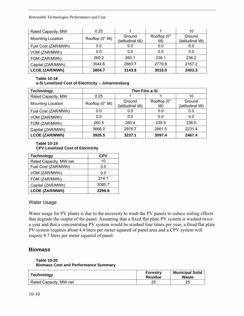
Renewable Technologies Performance and Cost
Rated Capacity, MW 0.25 1 1 10
Mounting Location Rooftop (0° tilt) Ground (latitudinal tilt)
Rooftop (0° tilt)
Ground (latitudinal tilt)
Fuel Cost (ZAR/MWh) 0.0 0.0 0.0 0.0 VOM (ZAR/MWh) 0.0 0.0 0.0 0.0
FOM (ZAR/MWh) 260.2 260.1 236.1 236.2
Capital (ZAR/MWh) 3544.6 2883.7 2779.9 2167.2 LCOE (ZAR/MWh) 3804.7 3143.8 3016.0 2403.3
Table 10-18 a-Si Levelized Cost of Electricity – Johannesburg
Technology Thin Film a-Si Rated Capacity, MW 0.25 1 1 10
Mounting Location Rooftop (0° tilt) Ground (latitudinal tilt)
Rooftop (0° tilt)
Ground (latitudinal tilt)
Fuel Cost (ZAR/MWh) 0.0 0.0 0.0 0.0 VOM (ZAR/MWh) 0.0 0.0 0.0 0.0
FOM (ZAR/MWh) 260.5 260.4 235.9 236.0
Capital (ZAR/MWh) 3666.0 2976.7 2861.5 2231.4 LCOE (ZAR/MWh) 3926.5 3237.1 3097.4 2467.4
Table 10-19 CPV Levelized Cost of Electricity
Technology CPV 10 Rated Capacity, MW net
Fuel Cost (ZAR/MWh) 0.0 VOM (ZAR/MWh) 0.0
214.1 FOM (ZAR/MWh) 2085.7 Capital (ZAR/MWh)
LCOE (ZAR/MWh) 2299.8
Water Usage
Water usage for PV plants is due to the necessity to wash the PV panels to reduce soiling effects that degrade the output of the panel. Assuming that a fixed flat plate PV system is washed twice a year and that a concentrating PV system would be washed four times per year, a fixed flat plate PV system requires about 4.4 liters per meter squared of panel area and a CPV system will require 8.7 liters per meter squared of panel.
Biomass
Table 10-20 Biomass Cost and Performance Summary
Technology Forestry Residue
Municipal Solid Waste
Rated Capacity, MW net 25 25
10-10

Renewable Technologies Performance and Cost
Plant Cost Estimates (January 2010) Total Plant Cost, Overnight, ZAR/kW 33,270 66,900 Lead Times and Project Schedule, years 3.5-4 3.5-4
Expense Schedule, % of TPC per year 10%, 25%, 45%, 20%
10%, 25%, 45%, 20%
Fuel Cost Estimates First Year, ZAR/GJ 19.5 0 Expected Escalation (beyond inflation) 0% 0% Fuel Energy Content, kJ/kg 11,760 11,390 Operation and Maintenance Cost Estimates Fixed O&M, ZAR/kW-yr 972 2,579 Variable O&M, ZAR/MWh 31.1 38.2 Availability Estimates Equivalent Availability 90% 90% Maintenance 4% 4% Unplanned Outages 6% 6% Performance Estimates Economic Life, years 30 30 Heat Rate, kJ/kWh 14,185 18,580 Plant Load Factor Typical Capacity Factor 85% 85% Maximum of Rated Capacity 100% 100% Minimum of Rated Capacity 40% 40% Water Usage Per Unit of Energy, L/MWh 210 200 Air Emissions, kg/MWh CO2 1287 1607 SOx (as SO2) 0.78 0.56 NOx (as NO2) 0.61 0.80 CO 1.52 2.00 Particulates 0.16 0.28 HCl 0.00 0.22 Solid Wastes kg/MWh Fly ash 24.2 1226 Bottom ash 6.1 3000
Table 10-21 Landfill Gas Reciprocating Engine Cost and Performance Summary
Technology Landfill Gas Rated Capacity, MW net 5 Plant Cost Estimates (January 2010) Total Plant Cost, Overnight, ZAR/kW 17,540 Lead Times and Project Schedule, years 1 Expense Schedule, % of TPC per year 100%
10-11

Renewable Technologies Performance and Cost
Fuel Cost Estimates First Year, ZAR/GJ 1.75 Expected Escalation (beyond inflation) 0% Fuel Energy Content, MJ/SCM 18.6 Operation and Maintenance Cost Estimates Fixed O&M, ZAR/kW-yr 497 Variable O&M, ZAR/MWh 111.1 Availability Estimates Equivalent Availability 86% Maintenance 5% Unplanned Outages 10% Performance Estimates Economic Life, years 20 Heat Rate, kJ/kWh 9,760-10,975 Plant Load Factor Typical Capacity Factor 85% Maximum of Rated Capacity 100% Minimum of Rated Capacity 12.5% Water Usage Per Unit of Energy, L/MWh 0 Air Emissions, kg/MWh CO2 806 NOx (as NO2) 0.6 CO 3 Particulates 0.24 VOC 0.8
Plant Cost Estimates
The total overnight cost for biomass plants burning forestry residue is estimated to be 33,270 ZAR/kW and 66,900 ZAR/kW for plants burning municipal solid waste. Because MSW boilers must be design to handle a much more diverse fuel input, they are built much more robustly. MSW boilers also require a scrubber, unlike a wood-fired boiler. For these reasons, the cost of the MSW plant is considerably higher than that of the forestry residue biomass plant. The total overnight cost for a landfill gas reciprocating engine is estimated to be 17,540 ZAR/kW.
It is expected that a biomass plant would have a 3.5 to 4 year expense and construction period. Early in the project, costs will include preliminary design, project siting, and permitting. Later in the project, equipment will be procured, delivered, and installed. This will be when the majority of the expenditures take place. The final stage of the project will be the commissioning of the plant. Based on this schedule, the expected expense schedule is 10% in year 1, 25% in year 2, 45% in year 3, and 20% in year 4.
The construction period for the landfill gas reciprocating engine is much shorter and is expected to be completed within a year. This is because the engine equipment is the bulk of the plant and
10-12

Renewable Technologies Performance and Cost
requires minimal siting and construction. This timeframe does not include the development of the landfill gas facility.
Fuel Cost Estimates
Forestry residue has a fuel energy content of about 11,760 kJ/kg. Municipal solid waste has a slightly lower energy content of 11,390 kJ/kg. Landfill gas has an energy content of 18.6 MJ/SCM. The cost of forestry residue is assumed to be 19.5 ZAR/GJ for this study. For municipal solid waste, the cost is assumed to be zero. In actuality, mass burn boilers are often paid to take municipal solid waste and the fuel cost can actually act as a credit for the plant. Figure 10-1 shows how the tipping fee for MSW can lead to negative fuel prices.
The landfill gas is assumed to be 1.75 ZAR/GJ for this study. The price of landfill gas can vary considerably and will depend on numerous variables, such as the quality, the quantity, the longevity of the gas supply, the potential of interruption of gas flow, the O&M arrangement on the gas collection and supply system, etc. The fact that a large landfill flares the landfill gas to waste if it is not utilized will depress the price that the landfill will charge the gas user substantially below the prevailing price of natural gas. Many landfill gas projects are developed and owned by the landfill owner. For such projects, there would be no fuel cost charged to the project, such as a power generation engine located on a landfill site that is owned and operated by the landfill owner.
10-13

Renewable Technologies Performance and Cost
Figure 10-1 Fuel Cost for MSW Based on Tipping Fee
Operation and Maintenance Cost Estimates
For a wood-fired biomass boiler, the fixed O&M is expected to be 972 ZAR/kW-yr and the variable O&M is expected to be 31.1 ZAR/MWh. For a MSW mass burn boiler, the fixed O&M is much higher due to the increased corrosive nature of the combustion products, as well as the additional emissions equipment. Fixed O&M is expected to be 2,579 ZAR/kW-yr and variable O&M is expected to be 38.2 ZAR/MWh for the mass burn MSW boiler. The fixed O&M for the landfill gas engines is 497 ZAR/kW-yr and the variable O&M is 111.1 ZAR/MWh. These landfill gas O&M costs are for the engines only and do not include O&M for landfill gas filtering or the compressor/blower, which could nearly double the variable O&M costs depending on the filtering required.
Availability and Performance Estimates
Both the wood-fired and MSW-fired plants have an expected availability of 90% and an expected capacity factor of 85%. The heat rate of the wood-fired plant is 14,185 kJ/kWh, while MSW plants have a higher heat rate of 18,580 kJ/kWh. The landfill gas engines have an expected
10-14

Renewable Technologies Performance and Cost
availability of 86%. This takes into consideration that at times the engines will not operate due to outages caused by the landfill gas supply company. The heat rate of the landfill gas engines is between 9,760 kJ/kWh and 10,975 kJ/kWh. As the load fluctuates, one, two or three of the four engines can be taken offline, resulting in the same full load heat rate at 75%, 50%, and 25% load. The high heat rate is associated with the minimum load of 12.5%. The economic life of both plants is expected to be about 30 years.
Cost of Electricity
Table 10-22 shows the levelized cost of electricity for the biomass plants. These are shown for illustrative purposes only and will vary based on financial assumptions.
Table 10-22 Biomass Levelized Cost of Electricity
Technology Forestry Residue
Municipal Solid Waste Landfill Gas
5 Rated Capacity, MW net 25 25 Fuel Cost (ZAR/MWh) 277.1 0.0 17.1 VOM (ZAR/MWh) 31.1 38.2 111.1
FOM (ZAR/MWh) 130.6 346.4 66.7
Capital (ZAR/MWh) 633.4 1259.4 298.7 LCOE (ZAR/MWh) 1072.1 1644.0 493.6
Water Usage
Because the steam cycles of these plants are air-cooled, the only water usage is for makeup water to the boiler. For both of the biomass boiler plants, this is about 227 L/MWh. The use of an air-cooled condenser reduces water consumption by over 90%. However, this leads to about a 7% derate penalty for an air-cooled plant compared to a wet-cooled plant, requiring that the rest of the plant, such as turbine generators and auxiliaries must be larger to generate the same amount of steam and output the same amount of electricity. Because there is no steam cycle for the landfill gas plant, there is no need for makeup water.
Emissions
Of the renewable technologies evaluated in this study, biomass plants are the only ones without zero emissions. Emissions are higher for the MSW plant than for the wood-fired plant, both because of the MSW is a dirtier fuel to start with and because of the higher heat rate of the MSW plant, which requires that more fuel is burned to generate the same amount of electricity. The air emissions and solid wastes, where applicable, are shown in the summary tables above.
10-15


11 GRID INTEGRATION AND INTERMITTENCY ISSUES FOR NON-THERMAL RENEWABLE TECHNOLOGIES
Managing significant quantities of renewable generation requires changes in the power delivery system at both the transmission and distribution levels. For example, at the transmission level, the variability of renewable resources will lead systems operators to redefine ancillary requirements, such as reserve requirements and ramp rates in order to operate the grid reliably. Operational changes may affect many tools and processes currently in use and will increase in importance for operators to meet reliability standards.
Because renewable technologies, especially solar and wind are not ‘dispatchable’, the practice in the US is to provide for gas turbines as a back-up in system reserve. In general, the regulatory agencies (Public Utility Commissions and Independent System Operators) in the US assign a value of about 10% to 15% of the total installed capacity of wind farms to the reserve margin (that is a 100 MW wind farm is assigned a 10 to 15 MW reserve margin capacity). Any shortfall in reserve margin is made up with gas turbines. Also, if there is regulatory stipulation that the maximum production capacity (up to 100%) of wind and solar be used this may require turning down some fossil units, which may lower their efficiency and increase emissions. Independent of this, the evaluations have only just begun on assessing the impact of the full use of renewable power generation capacity on fossil units, especially on pollution control units.
At the distribution level, the issues are different but equally important for enabling penetration of distributed generation into existing and future systems. These include evaluating interface devices, analytics, studies, applications with end-use resources, and assessment of new technology for effective interconnection and integration of renewable and other distributed generation. Recognizing the need for change and adapting the electric grid can enable higher penetration levels without reducing safety, reliability, or asset utilization effectiveness.
As a point of reference, in its 2008 Annual Report [1], the Electric Reliability Council of Texas (ERCOT, the agency responsible for managing electricity flow throughout the state of Texas) reported a peak load of 62 GW, average production of 35.6 GW, and 10 % installed capacity from wind generation. This portion of capacity represents a significant impact on the power system. Over 3 GW of wind capacity, at multiple locations, became operational in 2008.
ERCOT now has special operating procedures, extensive use of demand response, routine negative prices during low-load conditions, and investors, with government subsidies, are considering the introduction of energy storage pilot projects.
In its 2009 Annual Report [2], Eskom reported peak demand, not counting demand reductions, of almost 36 GW. Average production was about 20 GW out of 40 GW net maximum capacity. To reach 5% wind penetration by capacity, South Africa would need to install 2 GW or ten 200-MW wind farms. Technically, operational and planning impacts can be expected at this level of
11-1

Grid Integration and Intermittency Issues for Non-Thermal Renewable Technologies
penetration, and the evidence suggests that, depending on policy, such impacts could be expected within the energy planning horizon.
The costs cited in earlier chapters for renewable technologies include costs for thermal energy storage, power electronics, and reactive power compensation as appropriate. This chapter addresses other technologies that ease the integration of renewable energy into the electricity grid, which are mostly related to additional operating costs.
Technology Characteristics The primary challenges for the non-thermal renewable generation technologies considered in this study are variability and predictability of energy output. This section considers wind generation and photovoltaic technologies.
Wind Integration Issues
Grid integration of significant wind energy is expected to be the most challenging of all renewable options. The basic issue is wind turbine generators simply cannot perform all the functions that are expected from traditional generation.
Wind plant output varies with the weather and, by its nature, tends to be remote from load centers. Experience to date has shown that wind output is not likely to coincide with peak load requirements and that there are interesting successes and significant challenges to absorbing higher levels of deployment. Over speed tripping due to storm fronts and under voltage tripping due to power system faults have led to some significant tripping events.
Another characteristic of wind generation is its high rate of change or ramping. Although large positive and negative changes in the wind are rare, there is a need to understand and plan for them, especially in remote and relatively weak grid conditions.
Photovoltaic Solar Integration Issues Compared to wind, solar energy may be easier to integrate into the electric grid. Good solar resources are more often close to load centers and are more likely to coincide with and be available during the daily load peak. One exception is the rapid rate of change in output that may occur as clouds pass over solar arrays.
By its nature, solar energy can be more available during the summer than winter. For most areas with summer peaking of demand, its generation profile has a good match with the load profile. Even so, seasonal and daily variations of available output affect the capacity factor and overall system economics.
Like wind, solar photovoltaic power output can be quite variable due to partly cloudy weather and storm fronts. This has been observed in desert systems as well as those located in more temperate climates. Significant changes in solar system output can occur as clouds are passing by because these systems do not normally have any built in stored energy. The ramp rates of solar PV are likely higher than those of wind generation. Due to the large volume of heat transfer fluids contained within solar thermal fields, ramp rates associated with parabolic trough and central receiver plants tend to be reduced due to thermal inertia.
11-2

Grid Integration and Intermittency Issues for Non-Thermal Renewable Technologies
As large scale PV systems are just now being deployed, the issue of ramp rates is getting considerable attention. A large ad-hoc group being led by the National Renewable Energy Lab in Golden, CO is leading this effort in conjunction with academia, solar technology providers and utility companies.
Integration issues When wind, solar PV, and other intermittent generation resources are part of the generation mix, operators must consider the unique characteristics of the generator when planning and operating the power system. The following six characteristics of intermittent generation are likely to require changes in planned unit commitment, economic dispatch, and operating reserves:
• Intermittency
• Ramping burdens
• Fluctuating power output
• Limited reactive power control
• Distributed generation
• Remote location of some renewable resources.
Intermittency The output of most traditional generators can be planned, as well as controlled, even minute-to- minute to meet the expected daily load and to balance or regulate load variations. Wind power output depends on the weather and is determined by time-varying wind speeds; its output varies day to day as well as from hour to hour and even minute to minute. Two wind facilities may have the same capacity rating and annual energy production; however, different wind regimes may result in very different hourly, daily, and seasonal operating schedules. Similarly, solar PV plant output depends on the solar resource for the day or hour, and can be greatly affected by passing clouds.
Ramping Burdens
Bringing in wind generation and solar PV usually means that additional flexibility will be required in other sources of electrical generation to accommodate sub-hourly ramps.
Grid stability requires to moment-to-moment balancing of the load and generation to maintain a constant frequency. Rapid changes in system loads are matched by quickly ramping generation up or down to balance load and generation in a five-to-10-minute timeframe. Also, some units are required to ramp more quickly, following an automatic generation control (AGC) signal to maintain system balance. Operators refer to this process as regulation and the time frame is in minutes.
A substantial load change may cause sudden changes in frequency to which speed governors on individual generator units must respond. The number of plants and their capacity to provide load balancing and regulation are limited in any power system. The challenge is to have sufficient energy balancing and regulating generation with ramp rates to meet the worst-case fluctuations.
11-3

Grid Integration and Intermittency Issues for Non-Thermal Renewable Technologies
Wind power outputs have significant spatial variations; outputs from nearby wind plants are correlated, but outputs from distant wind plants are not correlated. This spatial variation can provide smoothing of output in show time frames. Short-time fluctuations of wind power can be independent regardless of distance between wind plants. However, longer-time wind power fluctuations are more likely to be correlated for nearby wind power plants.
Fluctuating Power Output
Rapid changes in power system loading or in generation can also cause small voltage fluctuations that manifest themselves as light flicker. Voltage changes of 1% to 2% can cause visible flicker. Wind turbines can cause voltage fluctuations due to a number of natural weather and machine conditions. These include fluctuations in wind speed, cut-in or cut-out transients, tower shadow effects, wind shear, and pitching errors of blades. Another factor in flicker production is the type of generator, which include induction generators with fixed or variable poles, variable-speed through electronic power conversion with or without pitch control, directly connected synchronous generators, or synchronous generators connected through a converter.
Limited Reactive Power Control Depending on the type of generator, reactive power supplied or absorbed by a renewable generation facility may vary along with the real power output. For example, most wind turbines use induction rather than synchronous generators and therefore require external capacitors to provide reactive power, usually switched in discrete steps. Even with switched capacitors, reactive control to match wind power generation may still be an issue. Externally switched capacitors will probably satisfy the steady-state reactive power balance requirement for the system but will not address any dynamic VAR control needs. Dispatching reactive power to maintain transmission network voltage could place new requirements on controlled generating facilities or necessitate capital investment for reactive compensation equipment. The addition of power electronics into the wind system can provide both dynamic and static reactive power control.
In the case of inverter-connected solar PV, many systems do not have reactive power control. The reactive power output varies depending on line voltage and solar output. This variation can be quite different than the real power output and may require some form of utility control and penetration levels to increase.
Distributed Generation
Wind, solar, and other renewable generation are deployed both as large projects interconnected to the transmission system and as small distributed facilities connected to the distribution system. Even though wind is considered primarily as a bulk-generation resource, a growing number of installations are being deployed on distribution systems at or near smaller load centers. Because distributed systems are designed for one-way power flow, distributed generators require special arrangements for connection and protection.
Two types of distributed wind and solar applications are common. Some facilities use local distribution to collect energy from individual units and deliver it to the distribution system. Other facilities are more dispersed and are individually connected to the system. Integration
11-4

Grid Integration and Intermittency Issues for Non-Thermal Renewable Technologies
issues that may surface in these distribution scenarios are voltage regulation, coordination of protection, and interferences or harmonic flows along rights of way. In general, these are the same integration concerns that occur when any generation is added into the distribution system.
Remote Location of Some Renewable Resources
Although good quality renewable energy sites exist throughout the world, the best wind and solar resources are typically located relatively far from large load centers. In addition, sites selected for building large wind farms are likely to be away from population centers. This is not unique to wind. For example, other generation types such as hydro and coal-fired stations may also be located at significant distances from load centers. However, wind developments have tended to not consider the available transmission capacity to these sites nor include the transmission-related costs of taking the wind to market.
Integration Technologies for Distribution-Connected Renewable Generation Today’s electric distribution systems have evolved over many years in response to load growth and changes in technology. The largest single investment of the electric utility industry is in the distribution system. Most common are radial circuits fed from distribution substations designed to supply load based on customer demand requirements while maintaining an adequate level of power quality and reliability.
The system is designed to be fed from a single source. Protection is based on time-overcurrent relays and fuses that use nested time delays to clear faults by opening the closest protective device to a fault to minimize interruptions. It is designed to safely clear faults and get customers back in service as quickly as possible. In areas of high load density, network systems are common. These systems are fed by multiple transmission sources, and thereby provide high reliability. Both radial and network distribution systems have been designed to serve load, with little planning for generation connected at these levels.
Within the United States, circuit sectionalizing switches are manually controlled to restore load in unfaulted sections downstream from a failure. The system voltage is maintained in compliance with American National Standard Institute (ANSI) Std. C84-1, which specifies that service voltage be delivered within 5% of the system rated voltage. These systems are generally considered to be ready to support small photovoltaic installations without change, when the PV inverters meet appropriate standards, and the overall penetration levels are very low.
The design and technologies associated with today’s distribution systems impose important limits on the ability to accommodate rooftop solar and other distributed generation, end-user load management, distributed system controls, automation, and future technologies like plug-in hybrid electric vehicles (PHEV). A number of system characteristics lead to these limitations:
• Voltage control is achieved with devices (voltage regulators and capacitor banks) that have localized controls. These schemes work well for today’s radial circuits but they do not handle circuit reconfigurations and voltage impacts of local generation well. This results in limits on the ways circuits can be configured and important limits on the penetration of distributed resources. This also limits the ability to control the voltage on distribution circuits for optimizing of customer equipment energy efficiency.
11-5

Grid Integration and Intermittency Issues for Non-Thermal Renewable Technologies
• There is little communication and metering infrastructure to aid in restoration following faults on the system.
• There is no communication infrastructure to facilitate control and management of distributed resources that could include renewables, other distributed generation, and storage. Without communication and control, the penetration of distributed generation on most circuits will be limited. The distributed generation must disconnect in the event of any circuit problem, limiting reliability benefits that can be achieved with the distributed generators as well.
• There is no communication to customer facilities to allow customers and customer loads to react to electricity price changes and/or emergency conditions. Customer-owned and distributed resources cannot participate in electricity markets, limiting the economic payback in many cases. Communications to the customer would also provide feedback on energy use that has been shown to help customers achieve improved energy efficiency.
• The infrastructure is limited in the capacity to support new electrical demand such as home electronics and PHEVs. These new loads have the potential to seriously impact distribution system energy delivery profiles. Communication and coordinated control will be needed to effectively serve this new demand.
At the same time, the distribution system infrastructure is aging, resulting in concerns for ongoing reliability. Utilities are struggling to find the required investment just to maintain the existing reliability, much less achieve higher levels of performance and reliability. New automation schemes are being implemented that can reconfigure circuits to improve reliability, but these schemes do not achieve the coordinated control needed to improve energy efficiency, manage demand, and reduce circuit losses.
The bottom line is that today’s power distribution system has not been designed for distribution- connected PV or other high penetration of distributed generation. In the past this was not an issue, but today, with larger amounts of PV connecting to the electric system, we can expect new challenges in how distributed and variable generation can be safely and reliably interconnected.
In order to directly address the issues related to connecting large amounts of PV in the distribution system, four key areas will need to be addressed:
1. Voltage regulation practices
2. Overcurrent protection practices
3. Grounding practices
4. Switching and service restoration practices
Depending on the robustness of the existing design practices, the distribution system can handle some level of distributed renewable generation without modification. The basis for simplified interconnect rules such as California Rule 21 is that some level of robustness in existing distribution design allows connection without detailed engineering studies. Standards such as IEEE 1547-2003 and U.L. Inverter Test Standard 1741 evolved to enable connection without major design changes to the electric system.
11-6

Grid Integration and Intermittency Issues for Non-Thermal Renewable Technologies
In most areas today, distributed renewable generation is treated as negative load and the usual functions of generation are not expected or required. However, as PV deployments grow, feeder cases that cross the threshold are expected, requiring changes in operation rules such that the distribution generation will need to provide voltage support and eventually energy balancing. This is anticipated to occur initially on individual feeders with high penetration and later on at the substation and sub-transmission level.
Integration Technologies for Transmission-Connected Renewable Generation Transmission is normally subject to the control of system operations and balancing authorities. In deregulated markets this would be the Independent System Operator (ISO). In vertically integrated utility markets it is usually the utility that owns most of the transmission and/or generation in the region.
The transmission systems are designed and built for two-way power flow. Therefore, if capacity is available at the location of connection, renewable generation variability can be absorbed by the grid. However, with traditional generation, system operators assume that most of the available energy resources are “dispatchable” and therefore expect to be able to schedule generator output with a high probability of delivery of the specified output. For wind, solar and other intermittent generation, this assumption is less valid.
Depending on the location and the relative size of renewable output, absorbing variable generation ultimately leads to increased cost related to the impacts of intermittency, ramping, fluctuating output, lack of control, and remote location on transmission scheduling, system dispatch, network stability, load following, and load balancing.
Variable Generation Technical and Cost Challenges
Integration for Distribution-Connected Renewable Generation In the future, a more automated distribution system will interact with distributed energy resources including photovoltaic generation and battery systems. This will in turn enable better utilization of these resources and higher penetration. The changes in the distribution grid for high-penetration PV will likely include the following:
• Interactive Voltage Regulation and VAR Management: Utility voltage regulator and capacitor controls will be interactive with each other and the photovoltaic sources. A central controller will help manage the interactivity to ensure optimized voltage and reactive power conditions.
• Bulk System Coordination of Photovoltaic Generation for Market and Bulk System Control: Control of renewable generation from a dispatch center will be needed. This will allow renewable generation to participate and be aggregated into energy markets as well as allow for control to preserve system stability, power quality, and reliability at the bulk level.
• Protective Relaying Schemes Designed for Renewable Generation: The distribution system and sub-transmission will include more extensive use of directional relaying, communication based transfer trips, pilot signal relaying, and impedance-based fault-protection schemes (like
11-7

Grid Integration and Intermittency Issues for Non-Thermal Renewable Technologies
those used in transmission). These can work more effectively with multiple sources on the distribution system.
• Advanced Islanding Control: Extensively automated switchgear and renewable generation with enhanced islanding detection to improve capability for detecting unintentional islands. Also, these systems should be able to reconfigure the grid/renewable generation into reliability-enhancing “intentional islands.”
• Interactive Service Restoration: Sectionalizing schemes for service restoration allow distributed photovoltaic and other renewable generation to pick up load during the restoration process. Once separated, these must deal effectively with overloads from cold-load pickup and the current inrush required to recharge the system.
• Improved Grounding Compatibility: Consider new devices and architectures in both renewable generation and distribution that address grounding incompatibilities between power system sensing, protection, and harmonic flows. Examples of such techniques are:
– Control or limit ground fault overvoltage via relaying techniques or ancillary devices instead of effectively grounded renewable generation requirements.
– Harden the power system and loads to be less susceptible to ground fault overvoltage (increase voltage withstand ratings).
– Change protective relaying for ground faults so a high penetration of grounding sources does not affect the ground fault relaying.
– Change feeder grounding scheme or load serving scheme back to a grounded three-wire system.
Distributed Energy Storage: Energy storage of various forms will apply to correct temporary load/generation mismatches, regulate frequency, mitigate flicker, and assist advanced islanding functions and service restoration.
These system changes and technology upgrades represent an extensive investment on the part of electric utilities, rate payers and equipment manufacturers and a huge change in the way the power system is operated and designed. These changes will not come overnight and will require many decades to implement as well as considerable engineering planning and development to determine the balance of features and capabilities needed against cost and complexity of implementation. Nonetheless, these are the approaches needed to move to high-penetration PV, and the industry needs to begin work now on research and development so that the technologies, tools, and approaches will be available in a timely manner.
Integration for Transmission-Connected Renewable Generation The impacts of intermittent wind generation on both technical operating limits, and ancillary costs, are summarized in the EPRI Report, Survey of Wind Integration Study Results (EPRI 1011883, March 2006), covering North American sites. A related report also covers European Sites (EPRI 1012734, March 2007).
The North American report reviews the wind integration studies conducted for nine mainland systems. These studies include the following:
11-8

Grid Integration and Intermittency Issues for Non-Thermal Renewable Technologies
• NYSERDA-NYISO
• Xcel North-280 MW
• Xcel North-1500 MW
• Alberta Electric System Operator (AESO)
• Bonneville Power Administration (BPA)
• Southwest Public Service Company
• WE Energies
• Great River Energy
• PacifiCorp
The wind generation penetration levels considered in these studies range from 0.3% to 20% of system peak load. The majority of the study results show that wind penetrations up to 20% lead to regulating reserve requirements of 30% or less.
The potential increase in intra-hour load following burdens range from 3% to 15% with the exception of the one 49% study result. Likewise, the potential increase in inter-hour load following burden was found to range from approximately 5% to 22%. Also, the capacity credit allocated to wind generation is only addressed in two of the nine studies presented in the North America report, with the credit ranging from 15% to 27% of rated capacity.
Intra-hour load-following cost impacts are also relatively low, ranging from zero to forty cents per MWh of wind. The inter-hour load-following costs are generally more significant. For the studies where the inter-hour load-following costs were determined in isolation, the cost impacts were $2.50 - $3.50 per MWh of wind generation. In other studies, the inter-hour load following cost is embedded with the uncertainty costs determined from scheduling/unit commitment assessments, but the costs appear to be of the same general magnitude range requirements.
The associated cost impacts of the increased regulating reserve burdens vary from twenty cents to a couple of dollars per MWh of wind. Much of the variation is associated with the assumed cost of providing (or obtaining) regulating reserves.
The increase in the standard deviation for scheduling uncertainty ranges from 20% to 50%. The associated costs are in the $1.00 to $4.50 per MWh range. Only one study yielded costs in excess of $10/MWh. It should be noted that not all cost components were calculated for all studies. Nonetheless, the studies that did evaluate cost impacts for most time frames yielded costs in the same range.
Grid Planning and Operating Tools
New tools to enable grid operators to better visualize the real time status of the grid, and to anticipate contingencies, are needed to moderate additions of intermittent resources. Several tools and methods are being developed in this area:
• Forecasting tools to predict renewable energy output on a near-real timeframe and up to 24 to 72 hours in advance using measured and numerical weather wind and solar resource data and statistical techniques. The forecasts need to be accompanied by measures of uncertainty and
11-9

Grid Integration and Intermittency Issues for Non-Thermal Renewable Technologies
confidence levels for grid operators to use to commit adequate capacity, plan and schedule to meet energy requirements. Benefits include minimizing unscheduled power flows, real-time voltage and dynamic stability problems and preventing blackouts. Research scope should include the use of time-dependent optimal power flow techniques to develop adaptive strategies for real-time operation.
• Methods to evaluate the capacity value of an aggregation of intermittent generation, energy storage, and demand response providers, which allows for the coordinated dispatch and scheduling. This would involve energy markets to help balance the economics and risks in power system operations.
• Visualization for grid operation needs to be extended to cover intermittent generation in a geographical display, together with visualization of load and demand response capabilities and the effect they have on the transmission loadings, voltages and frequencies of the power grid. This concept, developed by EPRI, will provide greater wide-area situational awareness to operators. Control room visualization may be a key technology for increasing intermittent generation without significant cost or loss of grid reliability R&D to develop automation concepts on adaptive relay protection, and voltage instability load shedding to handle the integration of substantial amounts of intermittent generation.
References [1] Eskom 2009 Annual Report.
http://www.financialresults.co.za/eskom_ar2009/ar_2009/downloads/eskom_ar_2009.pdf [2] ERCOT 2008 Annual Report.
http://www.ercot.com/content/news/presentations/2010/ERCOT%25202008%2520Annual%2520Report.pdf
11-10

A ACRONYM LIST
AEO – Annual Energy Outlook AGC - automatic generation control AGR - advanced gas-cooled reactor ASU – air separation unit BOP – balance of plant BWR - boiling water reactor CHP - combined heat and power CPV – concentrating photovoltaic CR – central receiver CSP – concentrating solar power CCGT – combined cycle gas turbine CT – combustion turbine DNI – direct normal insolation dPEF - densified processed engineered fuel DSG - direct steam generation EDG - emergency diesel generator EIA – US Energy Information Administration EPR - evolutionary pressurized reactor ERCOT - Electric Reliability Council of Texas ESP - electrostatic precipitators FBC – fluidized bed combustion FF - fabric filters FGD – flue gas desulfurization GT – gas turbine HCE - heat collection element HRSG – heat recovery steam generator HTF - heat transfer fluid IGCC – integrated gasification combined cycle ISO - Independent System Operator LCOE – levelized cost of electricity LFG - landfill gas LNG – liquefied natural gas LSFO – limestone forced oxidation LWR – light water reactor MOX - mixed oxide
A-1

Acronym List
MSW - municipal solid waste NERSA – National Energy Regulator of South Africa NREL – National Renewable Energy Laboratory OCGT- open cycle gas turbine O&M – operation and maintenance PC – pulverized coal PEF - processed engineered fuel PHEV - plug-in hybrid electric vehicles PV – photovoltaic PWR - pressurized water reactor RCS – reactor coolant system RDF - refuse derived fuel RPV - reactor pressure vessel SAM – Solar Advisor Model SCA - solar collector assembly SCR - selective catalytic reduction SNCR - selective noncatalytic reduction SSG - solar steam generator STC – standard test conditions TCR – total capital required TES - thermal energy storage TMY – typical meteorological year TPC - total plant cost USD – US Dollar ZAR – South African Rand
A-2

B SOLAR GENERATION PROFILES
The figures below show the generation profiles for the four parabolic trough cases evaluated: no storage, 3 hours storage, 6 hours storage, and 9 hours storage for two time periods, a summer day (January 15) and a winter day (July 15). The charts show the thermal energy exiting the solar field (Q_SF(MW) in red), the thermal energy to the thermal energy storage (Q_to_TES in blue), the thermal energy from the thermal energy storage (Q_from_TES in green), the thermal energy to the power block (Q_to_PB in purple), the gross power output of the plant (E_gross in orange) and the net power output of the plant (E_net in yellow). It can be seen that as the amount of storage increases, the thermal energy available to the power block from the storage increases, which extends the operating period of the plant or allows the plant to reach maximum output more of the time. These are shown for illustrative purposes only.
No Storage – January 15
B-1

Solar Generation Profiles
No Storage – July 15
3 Hours Storage – January 15
B-2

Solar Generation Profiles
3 Hours Storage – July 15
6 Hours Storage – January 15
B-3

Solar Generation Profiles
6 Hours Storage – July 15
9 Hours Storage – January 15
B-4

Solar Generation Profiles
9 Hours Storage – July 15
B-5


Electric Power Research Institute3420 Hillview Avenue, Palo Alto, California 94304-1338 • PO Box 10412, Palo Alto, California 94303-0813 USA
800.313.3774 • 650.855.2121 • [email protected] • www.epri.com
The Electric Power Research Institute Inc., (EPRI, www.epri.com)
conducts research and development relating to the generation, delivery
and use of electricity for the benefit of the public. An independent,
nonprofit organization, EPRI brings together its scientists and engineers
as well as experts from academia and industry to help address challenges
in electricity, including reliability, efficiency, health, safety and the
environment. EPRI also provides technology, policy and economic
analyses to drive long-range research and development planning, and
supports research in emerging technologies. EPRI’s members represent
more than 90 percent of the electricity generated and delivered in the
United States, and international participation extends to 40 countries.
EPRI’s principal offices and laboratories are located in Palo Alto, Calif.;
Charlotte, N.C.; Knoxville, Tenn.; and Lenox, Mass.
Together...Shaping the Future of Electricity
© 2010 Electric Power Research Institute (EPRI), Inc. All rights reserved. Electric Power Research Institute, EPRI, and TOGETHER...SHAPING THE FUTURE OF ELECTRICITY are registered service marks of the Electric Power Research Institute, Inc.
Export Control RestrictionsAccess to and use of EPRI Intellectual Property is granted with the spe-
cifi c understanding and requirement that responsibility for ensuring full
compliance with all applicable U.S. and foreign export laws and regu-
lations is being undertaken by you and your company. This includes
an obligation to ensure that any individual receiving access hereunder
who is not a U.S. citizen or permanent U.S. resident is permitted access
under applicable U.S. and foreign export laws and regulations. In the
event you are uncertain whether you or your company may lawfully
obtain access to this EPRI Intellectual Property, you acknowledge that it
is your obligation to consult with your company’s legal counsel to deter-
mine whether this access is lawful. Although EPRI may make available
on a case-by-case basis an informal assessment of the applicable U.S.
export classifi cation for specifi c EPRI Intellectual Property, you and your
company acknowledge that this assessment is solely for informational
purposes and not for reliance purposes. You and your company ac-
knowledge that it is still the obligation of you and your company to make
your own assessment of the applicable U.S. export classifi cation and
ensure compliance accordingly. You and your company understand and
acknowledge your obligations to make a prompt report to EPRI and the
appropriate authorities regarding any access to or use of EPRI Intellec-
tual Property hereunder that may be in violation of applicable U.S. or
foreign export laws or regulations.