WORKING P A P E R

Poverty and Time Preference LEANDRO CARVALHO

WR-759

May 2010

This paper series made possible by the NIA funded RAND Center for the Study of Aging (P30AG012815) and the NICHD funded RAND Population Research Center (R24HD050906).

This product is part of the RAND Labor and Population working paper series. RAND working papers are intended to share researchers’ latest findings and to solicit informal peer review. They have been approved for circulation by RAND Labor and Population but have not been formally edited or peer reviewed. Unless otherwise indicated, working papers can be quoted and cited without permission of the author, provided the source is clearly referred to as a working paper. RAND’s publications do not necessarily reflect the opinions of its research clients and sponsors.

is a registered trademark.

Poverty and Time Preference

Leandro S. Carvalho∗

Rand

April, 2010

Abstract

This paper estimates the time preference of poor households in rural Mexico. I use data from

a program that randomly assigned communities to treatment and control and paid transfers

to poor households in treatment communities. The randomization implies that differences in

consumption between control and treatment households are due to the program. A buffer-stock

model predicts how the response of consumption to transfers depends on the discount factor. I

estimate this parameter by matching simulated to sample treatment effects on consumption. My

estimates being very low, I conclude that poor households are very impatient or a richer model

is needed.

JEL: D91, 012

Keywords: Simulation, Consumption, Time Preference, Randomized Experiment, Poverty

∗I am grateful to David Lee, Chris Paxson and Sam Schulhofer-Wohl for their advice and support. I am also indebted toSilvia Helena Barcellos, Angus Deaton, Bo Honore, Alisdair McKay, Ashley Ruth Miller, Felipe Schwartzman and seminarparticipants at CEMFI, Einaudi Institute of Economics and Finance, Princeton University, Rand Corporation, Universidad deAlicante, University of California at San Diego and University of Oxford. Email: carvalho@rand.org.

1

1 Introduction

Empirical evidence shows that the poor and the non-poor behave differently when it comes

to choices involving intertemporal trade-offs. The poor have lower saving rates (Attanasio

and Szekely 2000; Dynan, Skinner and Zeldes, 2004), invest less in their children’s education

(Behrman, Birdsall and Szekely 1998) and have more children (Schultz 2005). Economists

have long debated the underlying reasons for these differences (Duflo 2006) and have sug-

gested numerous explanations: (1) the poor might face lower returns to their investments

(Rosenzweig 1995, van de Walle 2003); (2) some investment opportunities might not be

available to the poor due to inefficiencies in credit markets or insurance markets (Banerjee

2001) and (3) the poor and the non-poor might have different preferences (Lawrance 1991;

Atkeson and Ogaki 1996; Ogaki and Atkeson 1997). In particular, the poor might be more

impatient than the non-poor.

The last explanation suggests that time preferences might be a mechanism that transmits

poverty across generations. Becker and Mulligan (1997) argue that parents can increase

their children’s discount factors by investing in education. Moreover, theory predicts that

impatient parents invest less in their children’s human capital (Lang and Ruud 1986). These

children, in turn, will develop time preferences that are more present-oriented. When they

reach adulthood, they will be less educated and more impatient parents. To investigate

whether this hypothesis has any merit, it is necessary to know whether the poor and the

non-poor – as adults – have different time preferences.

Previous studies (Hausman 1979; Lawrance 1991; Atkeson and Ogaki 1997; Gourinchas

and Parker 2002; Cagetti 2003; Harisson, Lau and Williams 2002; Tanaka, Camerer and

Nguyen 2006; Stephens and Krupka 2006) have investigated differences in time preferences

between poor and non-poor by comparing estimates for the two groups. These studies have

produced mixed results.1 However, one limitation of this research is that it is difficult to

distinguish between differences in time preferences, and differences in the economic environ-

1Hausman (1979), Lawrance (1991), Harisson, Lau and Williams (2002) and Tanaka, Camerer and Nguyen (2006) find thatthe poor have higher discount rates. Gourinchas and Parker (2002), Cagetti (2003) and Stephens and Krupka (2006) yieldinconclusive results while Ogaki and Atkeson (1997) find no differences in time preferences.

2

ments in which the poor and the non-poor live. For example, differences in intertemporal

choices of the two groups might be partly explained by the fact that the poor are more likely

to be liquidity constrained.2

In this paper, I estimate the discount factor of poor Mexican households living in rural

communities. I explicitly model liquidity constraints and I present estimates for a wide range

of interest rates and risk aversion parameters to address concerns that particular assump-

tions about the economic environment might drive my results. I also compare my estimates

of the discount factor with existing estimates for non-poor households from studies that use

similar methods. I use data from PROGRESA, a program that randomly assigned commu-

nities to “treatment” and “control” groups, and extended conditional cash transfers to poor

households in the treatment communities 18 months before those in the control communi-

ties. The random assignment implies that, in the absence of the program, there would not be

any differences in the consumption behavior of control and treatment households. A model

gives predictions on how treatment households would spend the experimental variation in

wealth over time as a function of households’ time preference. Specifically, I use the canon-

ical buffer-stock model of consumption to simulate the effects of PROGRESA transfers on

consumption at different discount factors. I estimate the discount factor using the method

of simulated minimum distance by matching simulated and sample treatment effects on log

consumption.

My empirical approach bridges two methods that have been used to measure time pref-

erences.3 The first approach elicits discount rates from subjects by asking them to make in-

tertemporal choices over hypothetical or real outcomes (Coller and Williams 1999; Harrison,

Lau and Williams 2002; Andersen et al 2008). The most common experimental procedure

asks respondents to choose between a smaller, more immediate reward and a larger, more

delayed reward. A benefit of this method is the researcher’s ability to control the terms of

the experiment. However, there are concerns about the external validity of these estimates.

2Alternatively, Carroll (1997) argued that Lawrance’s(1991) results might be partly explained by the faster labor incomegrowth of more educated households.

3See Frederick, Loewenstein and O’Donoghue (2002) for a review of the literature on estimating time preferences.

3

The second method uses observational data on individuals’ intertemporal choices. For ex-

ample, macroeconomists have estimated structural life-cycle consumption models using data

on consumption and wealth (Gourinchas and Parker 2002; Cagetti 2003).4 This approach

entails simulating the consumption-age or wealth-age profiles as a function of the parameters

of the model, which are estimated by matching the simulated and sample profiles. The limi-

tation of this method is that it assumes changes in consumption or wealth over the life cycle

are entirely due to optimizing behavior as predicted by the model. The approach I take –

using observational data that embeds experimental variation in wealth – addresses concerns

about confounding factors that arise in observational studies but avoids the concerns about

external validity that arise in many experimental studies.

My results indicate that poor rural households in Mexico are very impatient. My bench-

mark estimates for the annual discount factor range from 0.08 to 0.70. These estimates are

much lower than what is found for the much wealthier households in the United States.

Three recent articles (Gourinchas and Parker 2002; Cagetti 2003; Laibson, Repetto and

Tobacman 2007) use data from large U.S. household surveys to estimate the parameters of

a stochastic life-cycle consumption model using the method of simulated moments. Their

estimates of annual discount factors range from 0.92 to 0.99 and concentrate around 0.95.

I take these estimates for the U.S. as reflecting the time preference of non-poor households

and formally test whether households in my sample have an annual discount factor above

0.90. For almost all model specifications, I am able to rule out at a 1% significance level any

annual discount factor above 0.90.

The intuition for my result is as follows. PROGRESA transfers increased over the first

few semesters of the program. If households faced no liquidity constraints, they would have

smoothed consumption either by drawing down their own assets when the program started,

or by borrowing against future transfers. This behavior would have produced treatment

effects in consumption that declined over time, with larger increases in consumption in the

earlier periods of the program. However, the data do not show such a pattern. Instead,

4One strand of the literature estimates discount rates using data on the purchase of durable goods (e.g., Hausman 1979).Other studies estimate discount rates from wage-risk tradeoffs (Viscusi and Moore 1989).

4

the treatment effects on log consumption increased over time, implying an absence of con-

sumption smoothing. The observed pattern of treatment effects is consistent with borrowing

constraints working in concert with impatience. A key point is that patience governs the

stock of assets that households can use for consumption smoothing. Patient households

hold larger stocks of assets before the program, on average, and so can use their own assets

to smooth consumption even in the presence of borrowing constraints. Impatient house-

holds, who hold smaller stocks of assets, cannot. A high degree of impatience – implying

lower initial assets – is necessary to reconcile the model with the rising treatment effects in

consumption observed in the data.

The structure of the paper is as follows. Section 2 gives some background on PROGRESA.

Section 3 introduces the model. Section 4 discusses the identification strategy and the

method of simulated minimum distance. Section 5 presents the empirical results, and section

6 presents robustness checks. Section 7 concludes with a discussion of alternative models

that could be consistent with the data.

2 Background on PROGRESA

PROGRESA is a conditional cash transfer program in Mexico that pays cash transfers

to households which comply with the program requirements. To evaluate the program, a

randomized social experiment was conducted in its initial phase: 506 rural communities were

randomly assigned to either participate in the program or serve as controls. A census was

conducted in 1997 – before the start of the program – in control and treatment communities

to identify eligible families.5 Eligible households in treatment communities started receiving

transfers 18 months before eligible households in control communities.

PROGRESA’s cash transfers have two major components: a scholarship conditional on

85% or higher attendance of school-age children, and a cash transfer for food that is condi-

tional on mandatory visits of household members to health clinics.6 The payments are made

5Households were classified as eligible/poor based on a measure of household’s permanent income rather than income reportedat the baseline survey. For more details, see Skoufias, Davis and Behrman (1999).

6Households also get twice a year support for school supplies. Households are not required to spend the transfer on food or

5

every two months. Hoddinott, Skoufias and Washburn (2000) report that average trans-

fers corresponded to roughly 20% of average expenditures of eligible households in control

communities. I do not model the program conditionalities and the household’s participation

decision. A majority (approximately 90%) of eligible households in treatment communities

enrolled in the program (Gertler, Martinez and Rubio-Codina 2006).

Treatment households started receiving transfers in May 1998.7 Households in control

communities were not incorporated into the program until November 1999 and started re-

ceiving transfers in December 1999. Control households were not notified about the program

until two months before incorporation and surveyors were told to conceal that the survey

was related to PROGRESA.8

3 The Model

3.1 Theoretical Model

The framework is a standard discrete-time intertemporal allocation problem (Deaton 1991a).

Infinitely-lived households maximize their lifetime utility:9

max{Ci,t+k}∞

k=0

Et

[ ∞∑k=0

βku (Ci,t+k)

], (1)

where u is instantaneous utility, β is the discount factor, C is consumption, t indexes time

and i indexes the household. Every period, households receive stochastic labor income Yi,t –

which is the only source of uncertainty – and some of them receive a positive cash transfer

Bi,t. There is a single asset in the economy with a constant gross real interest return R, and

school-related expenses. See Skoufias (2005) for more details.7They were told that benefits would be paid for three years and that their status would not change irrespective of changes

in household income. The existence of the program could not be guaranteed beyond 2000 because of the 2000 general election.8There is some controversy on whether control households anticipated participation in the program. See Attanasio et al

(2004), Skoufias (2005) and Todd and Wolpin (2006).9The majority of households in the sample are young couples with school-age children and are mostly saving for precautionary

reasons rather than for retirement. Carroll (1997) shows that, for the U.S., the infinite-horizon model is a good approximationto the finite horizon model up to age 50.

6

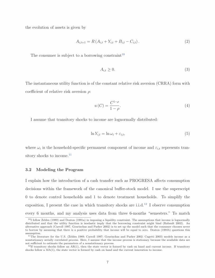
the evolution of assets is given by

Ai,t+1 = R (Ai,t + Yi,t + Bi,t − Ci,t) . (2)

The consumer is subject to a borrowing constraint10

Ai,t ≥ 0. (3)

The instantaneous utility function is of the constant relative risk aversion (CRRA) form with

coefficient of relative risk aversion ρ:

u (C) =C1−ρ

1− ρ. (4)

I assume that transitory shocks to income are lognormally distributed:

lnYi,t = lnωi + εi,t, (5)

where ωi is the household-specific permanent component of income and εi,t represents tran-

sitory shocks to income.11

3.2 Modeling the Program

I explain how the introduction of a cash transfer such as PROGRESA affects consumption

decisions within the framework of the canonical buffer-stock model. I use the superscript

0 to denote control households and 1 to denote treatment households. To simplify the

exposition, I present the case in which transitory shocks are i.i.d.12 I observe consumption

every 6 months, and my analysis uses data from three 6-months “semesters.” To match

10I follow Zeldes (1989) and Deaton (1991a) in imposing a liquidity constraint. The assumptions that income is lognormallydistributed and that the utility function is isoelastic imply that the borrowing constraint might bind (Rabault 2002). Analternative approach (Carroll 1997, Gourinchas and Parker 2002) is to set up the model such that the consumer chooses neverto borrow by assuming that there is a positive probability that income will be equal to zero. Deaton (1991b) questions thisassumption.

11The literature for the U.S. (Zeldes 1989; Carroll 1997; Gourinchas and Parker 2002; Cagetti 2003) models income as anonstationary serially correlated process. Here, I assume that the income process is stationary because the available data arenot sufficient to estimate the parameters of a nonstationary process.

12If transitory shocks follow an AR(1), then the state vector is formed by cash on hand and current income. If transitoryshocks follow a MA(1), the state vector is formed by cash on hand and the current innovation to income.

7

the frequency of the data, I assume that households solve their intertemporal problem on

a semi-annual basis. Henceforth, all discount factors presented are semi-annual discount

factors unless noted otherwise.

I assume that control households did not anticipate their participation in the program,

in which case their intertemporal allocation problem is the standard one. (I will relax this

assumption in section 6.) The value function of a control household is:

V 0 (Xi,t;ωi) = max{Ci,t+k}∞

k=0

u (Ci,t) + βEt

[V 0 (Xi,t+1;ωi)

], (6)

subject to constraints (2) and (3) and where Xi,t = Ai,t+Yi,t+Bi,t is cash on hand, the sum

of assets, income and transfers.

It is also initially assumed that treatment households did not expect the introduction

of the program but that, once the program was announced, households had no uncertainty

about the levels of transfers in future periods. Treatment households perfectly forecast

transfers two semesters ahead and expect transfers to remain constant from there into the

future. I model the seasonality in transfers – transfers are smaller in one semester because

households are not entitled to scholarships during the school holiday period – by letting

households have different expectations for each semester.13

Treatment households expect the program to last for 6 semesters, after which they expect

to stop receiving cash transfers. The value function of treatment households who have τ

periods remaining until the end of the program is:

V 1,τ (Xi,t, Bi,t+1, Bi,t+2;ωi) = max{Ci,t+k}∞

k=0

u (Ci,t)+βEt

[V 1,τ−1 (Xi,t+1, Bi,t+2, Bi,t+3;ωi)

], (7)

subject to constraints (2) and (3), where τ = max {7− t, 0}. At the end of the six semesters

– i.e, when τ = 1 – the value function of a treatment household is equal to the value function

13Define the “summer” semester as the six-months period from May to October and the “winter” semester as the period fromNovember to April of the following year. Let t = 1 denote the first semester of the program, from May to October of 1998,so odd periods denote summer semesters and even periods denote winter semesters. Thus, in the summer semester of 1998,treatment household i expects to receive in future winter semesters Bi,2 (the winter semester of 1998 actual transfers) and infuture summer semesters Bi,3 (the summer semester of 1999 actual transfers). Similarly, in the winter semester of 1998 (t = 2),household i expects to receive in future summer semesters Bi,3 (the summer semester of 1999 actual transfers) and in futurewinter semesters Bi,4 (the winter semester of 2000 actual transfers).

8

of a control household:

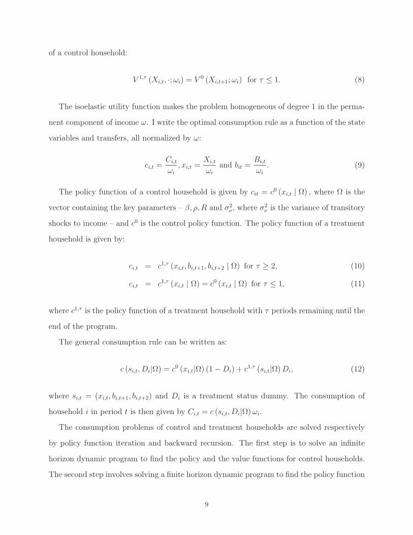
V 1,τ (Xi,t, ·;ωi) = V 0 (Xi,t+1;ωi) for τ ≤ 1. (8)

The isoelastic utility function makes the problem homogeneous of degree 1 in the perma-

nent component of income ω. I write the optimal consumption rule as a function of the state

variables and transfers, all normalized by ω:

ci,t =Ci,t

ωi

, xi,t =Xi,t

ωi

and bit =Bi,t

ωi

. (9)

The policy function of a control household is given by cit = c0 (xi,t | Ω) , where Ω is the

vector containing the key parameters – β, ρ, R and σ2ν , where σ

2ν is the variance of transitory

shocks to income – and c0 is the control policy function. The policy function of a treatment

household is given by:

ci,t = c1,τ (xi,t, bi,t+1, bi,t+2 | Ω) for τ ≥ 2, (10)

ci,t = c1,τ (xi,t | Ω) = c0 (xi,t | Ω) for τ ≤ 1, (11)

where c1,τ is the policy function of a treatment household with τ periods remaining until the

end of the program.

The general consumption rule can be written as:

c (si,t, Di|Ω) = c0 (xi,t|Ω) (1−Di) + c1,τ (si,t|Ω)Di, (12)

where si,t = (xi,t, bi,t+1, bi,t+2) and Di is a treatment status dummy. The consumption of

household i in period t is then given by Ci,t = c (si,t, Di|Ω)ωi.

The consumption problems of control and treatment households are solved respectively

by policy function iteration and backward recursion. The first step is to solve an infinite

horizon dynamic program to find the policy and the value functions for control households.

The second step involves solving a finite horizon dynamic program to find the policy function

9

for treatment households, where the horizon is equal to six semesters, the expected duration

of the program. The terminal value of the treatment household problem is given by the value

function of control households.

3.3 The Income Process

The data generating process for observed household income is assumed to be:

lnY ∗i,t = lnYi,t + ξi,t = lnωi + εi,t + ξi,t, (13)

where Y ∗i,t is observed household income, Yi,t is actual household income, ωi is household

permanent income, εi,t captures transitory shocks to income and ξi,t is measurement error.

I decompose permanent income into household size and per capita permanent income –

lnωi = lnhhsizei+lnμi – and assume that lnμi,t is normally distributed with mean lnμ and

variance σ2lnμ. The program identified eligible households by choosing the ones more likely

to be poor based on a proxy for per capita permanent income. Thus, I assume that lnμ is

distributed among eligible households as a truncated normal with mean lnμ and variance

σ2lnμ bounded above by some threshold level b.

Transitory shocks and measurement error are independent of permanent income. Mea-

surement error is serially uncorrelated and normally distributed with mean zero and variance

σ2ξ . The distribution of the transitory shock εi,t depends on the income process.14

14More precisely,

iid : εi,t = νi,t,

AR (1) : εi,t = ηεi,t−1 + νi,t,

MA (1) : εi,t = ηνi,t−1 + νi,t,

where νi,t˜iidN

(0, σ2

ν

).

10

4 Methodology

4.1 Identification Strategy

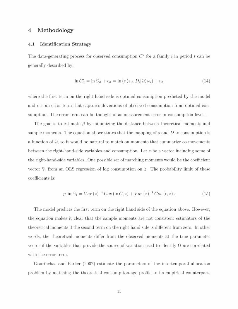
The data-generating process for observed consumption C∗ for a family i in period t can be

generally described by:

lnC∗it = lnCit + εit = ln (c (sit, Di|Ω)ωi) + εit, (14)

where the first term on the right hand side is optimal consumption predicted by the model

and ε is an error term that captures deviations of observed consumption from optimal con-

sumption. The error term can be thought of as measurement error in consumption levels.

The goal is to estimate β by minimizing the distance between theoretical moments and

sample moments. The equation above states that the mapping of s and D to consumption is

a function of Ω, so it would be natural to match on moments that summarize co-movements

between the right-hand-side variables and consumption. Let z be a vector including some of

the right-hand-side variables. One possible set of matching moments would be the coefficient

vector γ1 from an OLS regression of log consumption on z. The probability limit of these

coefficients is:

p lim γ1 = V ar (z)−1Cov (lnC, z) + V ar (z)−1Cov (ε, z) . (15)

The model predicts the first term on the right hand side of the equation above. However,

the equation makes it clear that the sample moments are not consistent estimators of the

theoretical moments if the second term on the right hand side is different from zero. In other

words, the theoretical moments differ from the observed moments at the true parameter

vector if the variables that provide the source of variation used to identify Ω are correlated

with the error term.

Gourinchas and Parker (2002) estimate the parameters of the intertemporal allocation

problem by matching the theoretical consumption-age profile to its empirical counterpart,

11

which is equivalent to having as z a vector of age dummies. Their identifying assumption

is that the error term is uncorrelated with age. But if there are other explanations for why

observed consumption evolves over the life cycle, the second term on the right hand side

of (15) will differ from zero. For example, the error term will be correlated with age if

there is time-varying measurement error in consumption or if omitted factors that determine

consumption vary over the life cycle.

In this article, I exploit the fact that the consumption behavior of control and treatment

households would have been the same in the absence of the program. In other words, any

treatment-control differences in consumption must be due to the program. I use the model to

predict program treatment effects on log consumption and match these to sample treatment

effects. In this case, z is a vector of time-treatment dummies.

I estimate the time preference of sample households from the following moment conditions:

E1[lnC∗

i,t

]− E0[lnC∗

i,t

]= E1 [ln c (si,t, Di|Ω0)ωi]− E0 [ln c (si,t, Di|Ω0)ωi] , (16)

where Ed [·] = E [·|D = d]. The expression on the left hand side is the sample treatment

effect on log consumption at period t while the expression on the right hand side is the

treatment effect predicted by the model. The identifying assumption is that the error term

ε is orthogonal to treatment status – i.e., E [εi,t | Di] = E [εi,t] .

The discussion above clarifies the advantage of using experimental variation to estimate

time preferences. When using changes in consumption over the life cycle to identify the

parameters of interest, the assumption is that the changes are entirely due to the optimizing

consumption behavior described by the model. This rules out any unobservables that are

correlated with age and with consumption. When using treatment-control differences in con-

sumption, the nature of the experiment implies that differences in the consumption profiles

of control and treatment households are due to the program. The model is used to describe

how treatment households’ consumption responds to the injection of PROGRESA transfers,

relative to the consumption of control households. The identifying assumption is that the

mean deviation of log observed consumption from log optimal consumption (as predicted by

12

the model) is the same for control and treatment households.

4.2 Simulated Minimum Distance

This section justifies the use of simulation methods and explains the simulation procedure.

The model presented in section 3 can be used to predict households’ consumption and to

calculate the theoretical moments (the treatment effects on log consumption predicted by

the model). The dataset, however, does not contain reliable data on households’ permanent

incomes nor on their wealth such that si,t in equation (12) is unobservable. Thus, s must be

integrated out of the moment conditions:

Ed [ln c (si,t, Di|Ω)] =∫

ln c (s,D|Ω) dFt (s; Ω | D = d) , (17)

where Ft is the cumulative distribution of s at date t conditional on treatment status D.

The consumption function does not have a closed form, so that (17) cannot be calculated

analytically. I follow Gourinchas and Parker (2002) in using a simulation method to overcome

this difficulty. The idea of these methods is to draw many realizations of s from dFt (·),compute ln c for each s, and calculate the mean of ln c across the simulated draws.

The simulation procedure involves three steps. First, for each household i and simulation

draw h, I generate a history of income shocks and draw per capita permanent income μhi

from the appropriate distribution. Second, I use the policy function of control households

and the history of income shocks to simulate the asset distribution at the eve of the pro-

gram.15 Finally, I simulate consumption after the program was introduced using different

policy functions for control and treatment households. The data on transfers and household

size required to simulate consumption come from the actual household-level data and are not

simulated. Average log consumption for the control (treatment) group is calculated as sim-

ulated log consumption averaged over control (treatment) households and simulation draws.

For any parameter Ω, the theoretical moment can be replaced by its simulated counterpart.

15The randomization implies that the asset distribution for control and treatment households should have been the samebefore the start of the program. The asset distribution is stationary and it can be simulated using the control policy function.

13

The simulation procedure in explained in greater detail in the appendix.

In estimating the model presented above, two complications emerge. First, the data

available are not rich enough to identify all the parameters of the model. In particular, there

is not enough variation in the data to estimate the risk aversion parameter and the interest

rate. Thus, I choose to present results for different values of the interest rate and the risk

aversion. Second, I follow Gourinchas and Parker (2002) in employing a two-stage estimation

procedure to estimate the parameters of interest. In the first stage, I use income data to

estimate the variance of log permanent income and the variance of transitory shocks. In the

second stage, I use the treatment effects on log consumption to estimate the discount factor

and the mean of permanent income.

More formally, let us define ψ =(σ2ν , σ

2lnμ

)and θ =

(lnμ, β

). The parameter vector ψ

is estimated in the first stage while θ is estimated in the second stage. Notice that θ is a

function of ψ as well as ρ and R since θ will be estimated conditional on particular values

for the interest rate and the risk aversion parameter.16

I proceed by defining gt, the difference between simulated treatment effects and sample

treatment effects on log consumption:

gt (θ, κ) =(E1 [lnC∗

it]− E0 [lnC∗it])− (

E1 [lnCit (θ, κ)]− E0 [lnCit (θ, κ)]), (18)

where κ =(ψ, ρ, R

).

The Simulated Minimum Distance estimator is given by:

θSMD = argminθg (θ, κ)′W ∗g (θ, κ) , (19)

where g (θ, κ) = [g1 (θ, κ) g2 (θ, κ) g3 (θ, κ)]′ – the three periods referring to the three

semesters during which the program was randomized – and the optimal weighting matrix

W ∗ is calculated from survey data. The variance-covariance estimator and its derivation is

contained in Appendix D.

16The standard errors presented in section 5 do not correct for the first stage estimation.

14

5 Empirical Analysis

5.1 Data

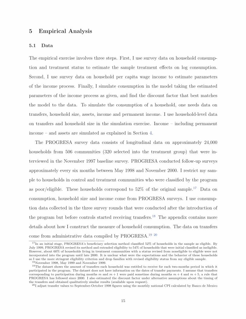
The empirical exercise involves three steps. First, I use survey data on household consump-

tion and treatment status to estimate the sample treatment effects on log consumption.

Second, I use survey data on household per capita wage income to estimate parameters

of the income process. Finally, I simulate consumption in the model taking the estimated

parameters of the income process as given, and find the discount factor that best matches

the model to the data. To simulate the consumption of a household, one needs data on

transfers, household size, assets, income and permanent income. I use household-level data

on transfers and household size in the simulation exercise. Income – including permanent

income – and assets are simulated as explained in Section 4.

The PROGRESA survey data consists of longitudinal data on approximately 24,000

households from 506 communities (320 selected into the treatment group) that were in-

terviewed in the November 1997 baseline survey. PROGRESA conducted follow-up surveys

approximately every six months between May 1998 and November 2000. I restrict my sam-

ple to households in control and treatment communities who were classified by the program

as poor/eligible. These households correspond to 52% of the original sample.17 Data on

consumption, household size and income come from PROGRESA surveys. I use consump-

tion data collected in the three survey rounds that were conducted after the introduction of

the program but before controls started receiving transfers.18 The appendix contains more

details about how I construct the measure of household consumption. The data on transfers

come from administrative data compiled by PROGRESA.19 20

17In an initial stage, PROGRESA’s beneficiary selection method classified 52% of households in the sample as eligible. ByJuly 1999, PROGRESA revised its method and extended eligibility to 54% of households that were initial classified as ineligible.However, about 60% of households living in treatment communities with a status revised from noneligible to eligible were notincorporated into the program until late 2000. It is unclear what were the expectations and the behavior of these householdsso I use the more stringent eligibility criterion and drop families with revised eligibility status from my eligible sample.

18November 1998, May 1999 and November 1999.19The dataset shows the amount of transfers each household was entitled to receive for each two-months period in which it

participated in the program. The dataset does not have information on the dates of transfer payments. I assume that transferscorresponding to participation during months m and m + 1 were paid sometime during months m + 4 and m + 5, a rule thatPROGRESA has followed since 2000. I also estimated the discount factor under alternative assumptions about the timing ofthe transfers and obtained qualitatively similar results (available upon request).

20I adjust transfer values to September-October 1998 figures using the monthly national CPI calculated by Banco de Mexico

15

5.2 Estimating the parameters of the Income Process

The income process presented in section 3 implies the following theoretical moments:21

V arE

(ln

Y ∗it

hhsizei

)= V arE (lnμ) + ϕ0σ

2ν + σ2

ξ ,

CovE

(ln

Y ∗it

hhsizei, ln

Y ∗it−1

hhsizei

)= V arE (lnμ) + ϕ1σ

2ν ,

where the subscript E indicates that the moments are calculated for the eligible population

and ϕ0 and ϕ1 depend on the process of transitory shocks.22 The parameters of the income

process can be estimated by minimizing the distance between the theoretical and empirical

moments.

In practice, I restrict the sample to eligible households and compute the sample vari-

ance and autocovariance of order 1, calculating separate moments for control and treatment

households.23 The variance of transitory shocks to income and the (cross-sectional) variance

of log permanent income are estimated using minimum distance estimation.24 The estimates

and for each household summed the values received in a given semester.21In Section 2, I discussed how households were classified as eligible or non-eligible based on a proxy for their permanent

income. Thus, the log permanent income is assumed to be distributed among the eligible population as a truncated normal.The variance of the unconditional distribution is given by:

σ2lnμ = V ar (lnμi) =

V arE (lnμi)[1− αγ (α)− [γ (α)]2

] , (20)

where α = Φ−1 (.52), .52 is the fraction of households who were deemed eligible, Φ is the standard normal cdf and γ is theMills ratio.

22More precisely,

i.i.d. : ϕ0 = 1;ϕ1 = 0,

AR(1) : ϕ0 =1

1− η2;ϕ1 =

η

1− η2,

MA(1) : ϕ0 = 1 + η2;ϕ1 = η.

23The U.S. literature (Carroll and Samwick 1997, Gourinchas and Parker 2002) has estimated income uncertainty fromwithin-household changes in income over time. Data limitations prevent me from using the same strategy here. First, thereis an intrinsic difficulty in measuring income of rural households in a developing country given that a large fraction of thesehouseholds is engaged in subsistence agriculture or self-employment. Second, the survey instrument used to collect income datachanged during the period of analysis. In particular, data on farming and livestock income were collected in only 2 surveyrounds. Finally, in each survey round, a large fraction of households reports no income. Given these limitations, I use datafrom five survey rounds on household (per capita) wage income, whose survey instrument was not modified across surveys.The goal is to provide a ballpark estimate of the uncertainty faced by the households in the sample. Nevertheless, it is a realconcern that the variability in wage income data might not accurately reflect the income uncertainty they face. Therefore, inthe robustness section, I vary the parameters of the income process drastically and show how the results are affected.

24The mean of log permanent income is estimated jointly with the discount factor in the second stage. Estimating the meanof permanent income is important because in many household surveys in developing countries income seems to be underreportedrelative to expenditures.

16

of the parameters of the income process are presented in Table 2 in the Appendix.25 The

variance of measurement error is estimated by assuming a reliability ratio λ of 0.7.26

5.3 Simulated Treatment Effects

Before moving on to the empirical analysis, I present results from simulations of the model.

These results provide intuition on the economics behind the empirical results, which I present

in the next section.

In a buffer-stock model, risk-averse households accumulate assets to use as a buffer against

income shocks. However, accumulating assets is costly because it reduces current consump-

tion. The more impatient households are, the more willing they are to substitute current

consumption for future consumption, and the less assets they will hold.

Treatment households had to decide how to change their consumption in response to

the exogenous increase in wealth. As shown in Appendix Table 1, transfers increased over

the first few semesters of the program. They increased roughly 150% between the first and

second semesters and 18% between the second and third semesters. If treatment households

anticipated rising transfers, they would have tried to smooth consumption. In particular,

impatience would have led them to run down their assets in the first semesters of the program

and let consumption fall over time. As a consequence, treatment effects in consumption

would have declined over time.

The previous intuition relies – given the borrowing constraints – on households having

enough assets to smooth consumption. But in a buffer-stock model, households’ asset hold-

ings are a function of their time preferences. The more impatient households are, the less

willing they are to forego current consumption to accumulate buffer wealth, and hence the

lower their assets will be on the eve of the program. Figure 1 in the Appendix presents the

simulated pre-program asset distribution for three different discount factors: 0.5, 0.75 and

0.9.27 Patient households hold, on average, more assets. The relationship of asset holdings

25In the AR(1) and MA(1) cases, I estimate V arE (lnμ) and σ2ν conditional on particular values of η: .25 and .5.

26The reliability ratio is defined as λ = V arE

(ln Yit

hhsizei

)/V arE

(ln

Y ∗it

hhsizei

). Bound and Krueger (1991) find that the

reliability ratio in US cross-sectional data is 0.82 for men and 0.92 for women.27For more details on how the asset distribution is simulated, see Appendix.

17

to time preferences has important implications. When the program is introduced, treatment

households want to smooth consumption in anticipation of higher future transfers. However,

because households cannot borrow, they must use their own assets to finance any increase in

first-semester consumption that exceeds the first-semester transfer. A high degree of impa-

tience implies that households cannot easily do so because they have a small stock of initial

assets; in this case, treatment households’ consumption will track transfers over time.

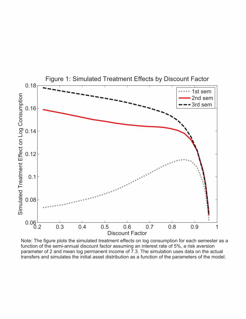
Figure 1 plots simulated treatment effects on log consumption against the (semi-annual)

discount factor for the first three semesters of the program.28 The distances between the

curves tell how the windfall is distributed over time. The graph shows that the increase

in treatment households’ consumption is roughly evenly distributed over time if households

have a high discount factor, but not if households are less patient.29

Finally, I present the time profile of treatment effects. Figure 2 plots the simulated

treatment effects against the program semester for three different discount factors: 0.5,

0.75 and 0.9. The profile is positively sloped. Because of borrowing constraints, treatment

households’ consumption – and the treatment effects – grow over time following the growth

in transfers. Moreover, patient households have larger initial assets and are more able to

smooth consumption over time. As a consequence, the time profile of simulated treatment

effects is flatter for higher discount factors.

Figure 2 also shows the program treatment effects on log consumption estimated from

survey data, which give rise to a steep profile. The comparison of the sample treatment

effects with the simulated treatment effects suggests that the two can be matched only if

households have a low discount factor.28The simulation uses household-level data on actual transfers.29In the second and third semesters, the treatment effect is decreasing in the discount factor because more patient households

have a lower marginal propensity to consume out of transfers. The treatment effect is non-monotonic in the first semester becausehouseholds want to increase consumption by more than the transfers in anticipation of higher future transfers. Households haveto finance an increase in consumption which exceeds the first semester transfers using their pre-program asset holdings – whichis as increasing function of the discount factor – given that they cannot borrow against future transfers.

18

5.4 Results

5.4.1 Sample Treatment Effects

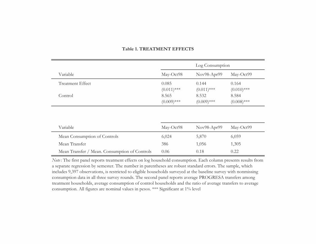
Table 1 presents the program treatment effects on log consumption estimated from the survey

data. I will estimate the discount factor by matching simulated treatment effects to these

sample treatment effects. The top panel of Table 1 reports the estimates of a regression

of household log consumption on treatment status, by program semester.30 The treatment

effects rise over time, from 8.5% for the first semester of the program, to 14.4% in the second

semester, to 16.4% for the third semester.31

The second panel of Table 1 reports average PROGRESA transfers for the treatment

group and average consumption in levels for the control group. The last row of the panel

shows the ratio of average transfers to control average consumption, which can be compared

to the treatment effects. If the treatment effect is higher than the ratio of transfers to control

consumption, this suggests that treatment households increased their consumption by more

than the transfer. The treatment effect was higher than the ratio of transfers to control

consumption in the first semester, but lower in the second and third semesters.

5.4.2 Estimates of the Discount Factor

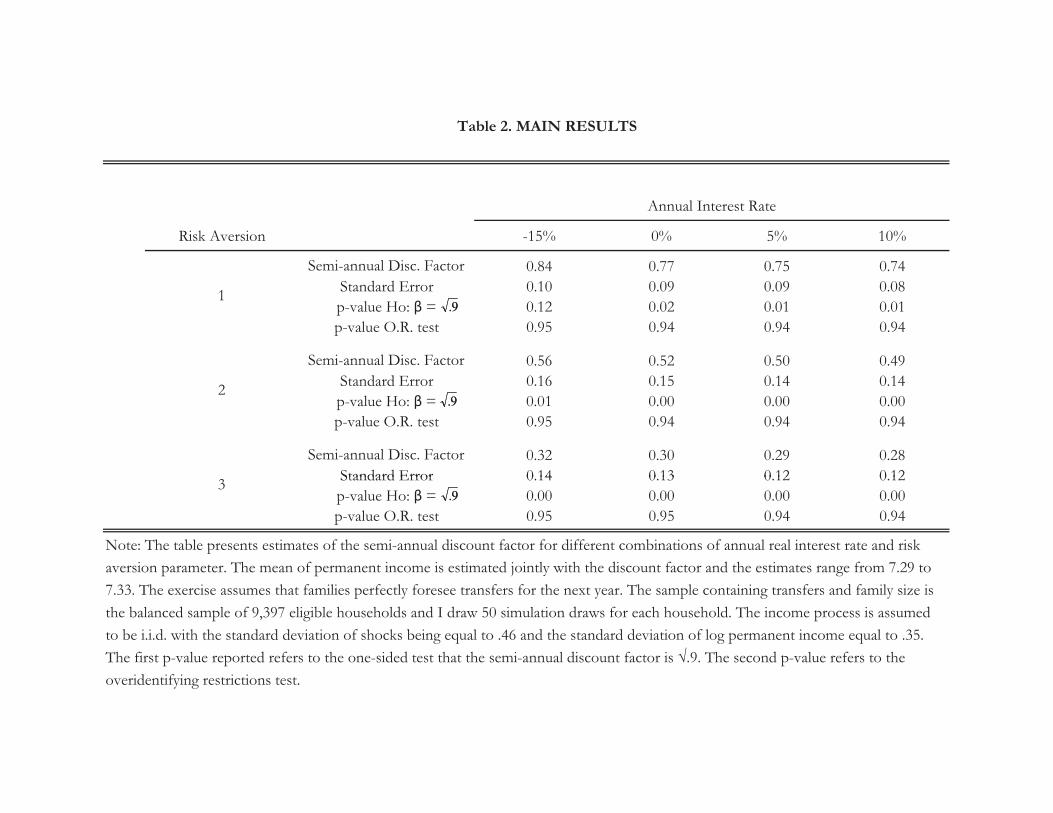
Table 2 presents my benchmark estimates of the discount factor.32 All estimates of the

discount factor are conditional on the interest rate and the risk aversion.33 They assume that

transitory shocks to income are independently identically distributed.34 The table displays

results for nine possible combinations of the interest rate and the coefficient of relative risk

aversion. The interest rate varies across columns while the risk aversion varies across rows.

I follow Laibson, Repetto and Tobacman (2007) and show results for three different risk

30The sample contains 9,397 observations with non-missing consumption data in all three survey rounds. In the simulation,I choose the missing observations to be exactly the same as in the observed data.

31These findings are consistent with other work (Stephens 2003; Shapiro 2004; Mastrobuoni and Weinberg 2009) which findthat recipients of government transfers such as Social Security checks and food stamps in the U.S. do not smooth consumptionbetween payment dates.

32Estimates of lnμ range from 7.29 to 7.33, which corresponds to an average ratio of transfers to income of about .2.Hoddinott, Skoufias and Washburn (2000) estimate that the ratio of average transfers to average expenditures of the controlgroup is 20%.

33As discussed in Section 4, I do not estimate the risk aversion parameter because I cannot separately identify the discountfactor from the risk aversion parameter.

34I also present results in Appendix Table 3 assuming that transitory shocks follow an AR(1) or MA(1) process.

19

aversion coefficients – 1, 2 and 3 – that are commonly used in lifecycle consumption models.35

I vary the interest rate over a wide range, from -15% to 10%. Annual inflation for the period

was approximately 15% and the real interest rate was 5%. The real interest rate would

have been -15% if households received no interest on their savings. For each combination of

risk aversion and interest rate, four figures are shown: the semi-annual discount factor, its

standard error, the p-value from a hypothesis test that the semi-annual discount factor is

equal to√0.9 (corresponding to an annual discount factor of .9) and the p-value from a test

of overidentifying restrictions.

The point estimates of the semi-annual discount factor in Table 2 suggest that households

are very impatient. The figures in the table have to be squared to obtain annual discount

factors. The highest semi-annual discount factor is 0.84, which corresponds to an annual

discount factor of 0.7 and to an annual discount rate of 43%. The lowest semi-annual discount

factor is 0.28, which corresponds to an annual discount factor of 0.08 and to an annual

discount rate of 1156%. Although the estimates vary according to the values of the risk

aversion parameter and the interest rate, all the estimates imply a high degree of impatience

and are well below the discount factors typically estimated for the U.S. For comparison,

Gourinchas and Parker (2002), Cagetti (2003) and Laibson, Repetto and Tobacman (2007)

apply similar methods to U.S. data and obtain estimates of the annual discount factor ranging

from 0.921 to 0.989.

Overall, it is hard to reconcile the behavior of poor rural households in my sample with

discount factors which have been estimated for the wealthier households in the U.S. Table 2

reports the p-value for the null hypothesis that the semi-annual discount factor is√.9 against

a one-sided alternative. I can reject the null at 5% for all combinations of risk aversion and

interest rate except one: the case with a negative interest rate of 15% and a risk aversion of

1. Despite the large standard errors, I can generally bound the estimates away from annual

discount factors above 0.9. 36

35See Laibson, Repetto and Tobacman (2007) for a discussion on the values of the risk aversion parameter.36I get similar results – in terms of being able to bound the estimates away from an annual discount factor above 0.9 – if

I compute 95% confidence regions based on the distribution of the objective function. More precisely, let θ be the parametervector that minimizes the objective function g′W ∗g as defined in equation (19) – for simplicity, I drop κ from the notation.

20

The estimates are sensitive to the risk aversion parameter but change little with the

interest rate. As explained in Section 5.3, households decide how much to consume by striking

a balance between their impatience and their precautionary motives. When households

are more risk averse, the precautionary motives for savings are stronger. If, for example,

households were risk neutral, they would have no assets at the eve of the program and

treatment households’ consumption would track transfers over time. This intuition explains

why there is a negative relationship between the discount factor that the data imply and

the risk aversion parameter. Similarly, households have more incentives to save when the

interest rates are higher, giving rise to a negative relation between the estimated discount

factor and the interest rate.

Finally, Table 2 reports a measure of model fit. I estimate two parameters using three

moments so there is one overidentifying restriction, which can be tested using a chi-squared

test. Table 2 reports the p-value from this test; I cannot reject the overidentifying restriction

at any conventional significance level.

6 Robustness Checks

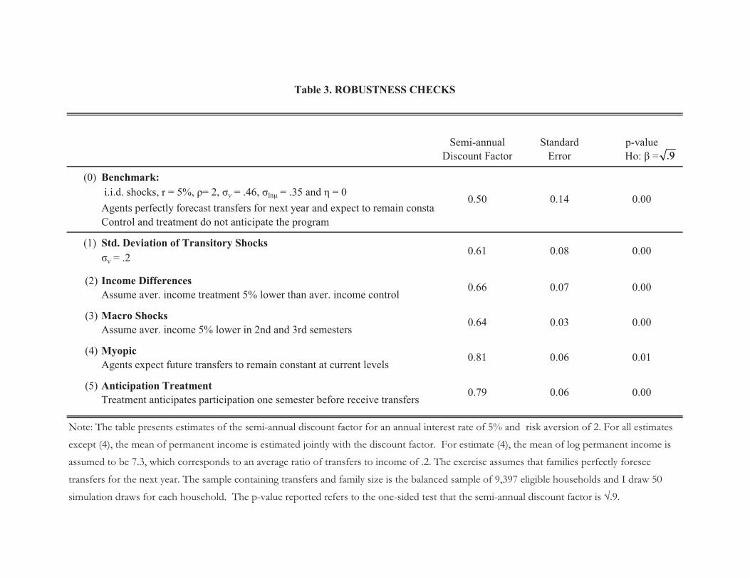
Table 3 examines how sensitive the results are to some of the assumptions of the benchmark

model.37 It presents robustness checks assuming an annual interest rate of 5% and a coef-

ficient of relative risk aversion parameter of 2.38 The first row, labeled row 0, repeats the

results for the benchmark case.39 The other rows present results for alternative assumptions.

The first column says which assumption is varied. The remaining columns present the semi-

annual discount factor estimate, its standard error and the p-value from a one-sided test of

the null hypothesis that the semi-annual discount factor is√0.9.

Define

ϑ (β) = minlnμ

g′(

lnμβ

)W ∗g

(lnμβ

)− g

(θ)′W ∗g

(θ).

The limiting distribution of the statistic ϑ (β) is chi-squared with one degree of freedom. The 95% confidence region is the setof β’s for which ϑ (β) is smaller than 3.84.

37Additional robustness checks are presented in Appendix Table 3.38I have also conducted robustness checks for other combinations of the interest rate (-15%, 0%, 5% and 10%) and the risk

aversion parameter (1, 2 and 3). These results are available upon request.39The benchmark assumes that transitory shocks are i.i.d. with standard deviation of .36, that the standard deviation of log

permanent income is .46 and that control and treatment households have the same income process.

21

The first three rows of Table 3 show results under alternative assumptions about the

income process. Row 1 reduces the standard deviation of transitory shocks from .36 to .2,

which is the estimate of Gourinchas and Parker (2002) from U.S. data.40 The estimate of the

discount factor is higher, but it remains low.41 Row 2 relaxes the assumption that control

and treatment households continued to have the same income process after the program

was introduced. It assumes that treatment households’ permanent incomes were on average

5% lower than control households’ permanent incomes.42 The estimate for the semi-annual

discount factor raises to 0.66 and the annual discount factor to 0.43 so that the annual

discount rate falls to 130%. Row 3 investigates whether macro shocks can explain the

growth of treatment effects over time. I estimate the discount factor assuming that there

was an unexpected aggregate shock of -5% to income of control and treatment households

in the second and third semesters of the program.43 The estimate of the annual discount

factor rises to 0.41 and the annual discount rate falls to 145%.

The remaining rows of Table 3 show how results change when alternative assumptions

are made concerning households’ expectations about the program. As explained in section

5.3, the results are driven by the growth in treatment effects over time. We would expect to

observe a similar pattern if households did not anticipate the growth in transfers but instead

revised their consumption plans upward as they received higher-than-expected transfers.44

Row 4 shows results for when treatment households have myopic expectations and expect

transfers to remain constant at the current level. The estimate is higher than for the bench-

mark case, but I can still reject an annual discount factor above 0.9 at the 5% level.45 Row 5

40I take their estimate as a lower bound for the income risk rural households in Mexico face.41Row 1 of Appendix Table 3 reduces the standard deviation of log permanent income from .35 to .15, which is the variance of

log permanent income estimated by Gourinchas and Parker (2002). In my model, the variance of log permanent income refers tothe time-invariant cross-section variance of log permanent income. Gourinchas and Parker (2002) estimate a within-householdtime variance of log permanent income, which I take to be a lower bound of the cross-sectional variance of my model.

42It is possible that PROGRESA reduced the income (excluding PROGRESA transfers) of treatment households because ofa reduction in child labor or because households enrolled in PROGRESA were not entitled to receive government transfers fromother programs. The evidence suggests that control and treatment households did not have different income processes (Parkerand Skoufias 2000; Gertler, Martinez and Rubio-Codina 2006; Angelucci and De Giorgi 2006; Albarran and Attanasio 2002;Gertler, Martinez and Rubio-Codina 2006).

43When hit by a negative income shock, treatment households use the transfers to buffer the shock. As a consequence, theconsumption of treatment households changes less than the consumption of control households. Thus, treatment effects areexpected to be larger in semesters with negative aggregate shocks.

44Row 2 of Appendix Table 3 assumes that treatment households were pessimistic about the continuation of the programand expected to receive zero transfers in the future.

45For myopic and pessimistic expectations, I cannot identify the discount factor separately from the mean log permanentincome. Hoddinott, Skoufias and Washburn (2000) estimate that the ratio of average transfers to average expenditures of the

22

assumes treatment households anticipated participation in the program one semester before

they started receiving transfers.46 The estimates increase to an annual discount factor of

0.62, corresponding to an annual discount rate of 61%.

7 Conclusion

My benchmark results indicate that poor households in rural Mexico have very low discount

factors, much lower than those found in U.S. data using similar methods. My result is

robust to a wide variety of alternative assumptions about households’ expectations and the

economic environment they face. To obtain discount factors similar to those in the U.S., I

would need to assume either that households have an unusually low degree of risk aversion

or that the households had mistaken beliefs about future transfers – which seems unlikely

because, government officials visited each community and explained the program at a public

meeting.

There are three possible interpretations of the results. The first is that the poor are

very impatient, which has implications both for policy design and for future research. First,

poverty reduction programs that try to increase poor households’ investments in human

capital will be more effective when part of the returns to these investments accrues in the

short run. Second, future research should investigate the underlying reasons for differences

in time preferences of poor and non-poor households.

The second interpretation is that the model does not contain a sufficiently rich description

of households’ information and the assets they can hold. In particular, the model abstracts

from uncertainty about future transfers and does not allow for the possibility that house-

holds hold illiquid assets. When there is uncertainty about future transfers, households are

reluctant to deplete their assets to increase consumption in anticipation of higher future

control group correspond to 20%. The results I present are estimated conditional on lnμ = 7.3, which corresponds to anaverage ratio of transfers to income of .2. Higher values of lnμ correspond to higher estimates of the discount factor but implyimplausible low values of average income given that expenditures provide a lower bound for income. Both of these models fitthe data worse than the benchmark model. I cannot reject the overidentifying restriction for myopic expectations, but I canreject it at 5% for pessimistic expectations.

46In this case, treatment households would have increased consumption at the time of the announcement by reducing theirbuffer wealth. Treatment households’ consumption would have tracked transfers more closely during the first three semestersof the program, implying a higher estimate of the discount factor.

23

transfers: they might not receive any transfers in the future and they would have no buffer

wealth to shield future consumption from income shocks. Another explanation is that house-

holds failed to smooth because they hold mostly illiquid assets, which they could not use

to substitute current consumption for future consumption.47 Households would choose to

hold few liquid assets if the returns to available liquid assets were sufficiently lower than the

returns to illiquid assets.

The third interpretation is that the very low estimated discount factors suggest that a

different model may be needed to describe the consumption behavior of poor households

in developing countries. The co-movement between treatment effects in consumption and

transfers observed in the data is, for example, consistent with sophisticated hyperbolic pref-

erences, which induce households to keep most of their savings in illiquid assets to cope with

their self-control problems (Laibson 1997).

47Rosenzweig and Wolpin (1993) note that most of the assets held by farmers are inputs to production but also serve asbuffer against income shocks. They propose a model in which investment assets are used both for production and to smoothconsumption.

24

Appendix

A Construction of Consumption Measure

I use the November of 1998, May of 1999 and November of 1999 survey rounds which collected data on

consumption. The module included questions on 36 food items and households reported for each of these

items expenditures, quantity consumed and quantity purchased in the last 7 days. The respondent was given

an option to report quantities in 3 units of measure: Kilos, Liter or Units. I exclude data on consumption

of alcohol, for which the data seems unreliable.

Household-specific prices were calculated by dividing expenditures by quantity purchased. I trimmed

prices which were below the 1st percentile or above the 99th percentile. If a household reported consuming

a give food item but the price was missing – either because of trimming, no quantity had been purchased

or because the measure unit of purchase was different from the measure unit of consumption – then the

household-specific price was set equal to the local price. Median prices at the village, municipality, state and

national level were calculated for each measurement unit and the local price was set equal to the lowest level

of aggregation with at least 20 household-specific price observations. The value of consumption for each item

was calculated as the product of prices times quantity consumed, where prices and quantities were quoted

in the same unit of measure. Household food consumption was calculated as the total value of consumption

over the 35 items and converted to a semi-annual figure.

Households were also asked to report their expenditures with 24 non-food items. I exclude data on

expenditures with weddings, funerals and ceremonies. The length of the reporting period was different

for different items: transportation costs (last 7 days); personal and house hygiene, drugs and prescriptions,

doctor visits, heating (i.e., wood, gas, oil), electricity (last month); clothing and shoes, school related expenses

(last 6 months). I converted the expenditures to semi-annual figures and summed over all expenditures to

calculate consumption of other goods.

Household total consumption is calculated as the sum of food consumption and consumption of other

goods. Finally, I trimmed the total consumption distribution in each survey round in 1%.

B Policy Function

I first solve the consumption problem for control households by using policy function iteration. I create

a grid for cash on hand x with 250 points. For each value of cash on hand on the grid I find the level of

consumption c which maximizes lifetime utility. The expected value of the value function one period ahead is

25

calculated by discretizing the shock and using a three-node Gaussian quadrature scheme. I use cubic spline

interpolation to approximate the policy function for levels of cash on hand between grid points.

The second step is to solve the consumption problem for treatment households using backward recursion.

Again, I create a grid for cash on hand identical to the one created for control households. For treatment

households, there is heterogeneity in the amount of transfers households receive. Thus, I proceed to create

a 7 by 7 grid corresponding to different levels of summer semesters and winter semesters transfers – b1 and

b2. Starting at period T − 1, for each value of cash on hand on the x grid and for each value of transfers on

the (b1, b2) grid I find the optimal consumption level – where period T is the last period in which households

expect to receive transfers. The terminal value function is given by the value function of control households.

The optimal consumption for periods before T − 1 are found recursively. I use cubic spline interpolation to

approximate the policy function.

C Simulation

In the simulation exercise, each household i is characterized by its treatment status Di, its history of transfers

{Bi,t}5t=1 and its household size hhsizei – all of which come from household-level data. I generate for each

household 50 fictitious histories of income shocks νhi,t and permanent (per capita) income μhi – where h indexes

the simulation draw. Notice that both of these variables are assumed to be independent of household size,

treatment status or transfers. Using the first 100 periods of each history and the control policy function,

I simulate for each household i and simulation draw h its initial asset level – i.e., the household’s financial

wealth at the beginning of the first semester of the program: ahi,t=1. I set ahi,−99 = 0 ∀i, h and run history

for 100 periods:

ahi,t+1 = R(ahi,t + yhi,t − chi,t

),

chi,t = c0(ahi,t + yhi,t|Ω

),

where tε {−99, ..., 0}.In the post-program period, control and treatment households have different policy functions. Consump-

tion for a control household i is simulated as:

Chi,t = c0

(ahi,t + yhi,t|Ω

) ∗ ωhi

26

while consumption for a treatment household i is simulated as:

Chi,t = c1,τ

(ahi,t + yhi,t, b

hi,t+1, b

hi,t+2|Ω

) ∗ ωhi ,

where:

τ = 7− t for tε {1, 2, 3} , bhi,t =Bi,t

ωhi

and ωhi = hhsizei ∗ μh

i .

The household size and the history of transfers {Bi,t}5t=1 are kept constant for a given household i across

simulation draws h. I then average log consumption across simulation draws h and households i for each

group. The treatment effect is the difference between the simulated average log consumption of treatment

and control households.

D Variance

The Simulated Minimum Distance Estimator is defined by:

θSMD = argminθ

g′ (θ, κ)W ∗g (θ, κ) .

The first-order condition for the second stage estimator is:

∂g′

∂θ

(θ, κ

)W ∗g

(θ, κ

)= 0.

Expanding g(θ, κ

)around θ0 and solving for θ − θ0 yields:

θ − θ0 = −[∂g′

∂θ

(θ, κ

)W ∗ ∂g

∂θ′(θ, κ

)]−1∂g′

∂θ

(θ, κ

)W ∗g (θ0, κ) .

For simplicity, I assume that the uncertainty of the first stage does not affect the uncertainty of the second

stage – i.e., ∂g′

∂κ (θ, κ) ≈ 0. I employ the optimal weighting matrix W ∗ = (V ar [Φ (θ0)])−1

, in which case

the Slutsky and central limit theories imply that θ − θ0 converges in distribution to a mean zero normal

distribution with asymptotic variance:

V ar(θ)=

[∂Φ′

∂θ(θ0)V ar [g (θ0)]

∂Φ

∂θ′(θ0)

]−1

, (21)

where Φ (·) are the theoretical moments corresponding to the sample moments g (·). The simulation inflates

the variance of the minimum distance estimator such that V ar [g (θ0)] =(1 + 1

H

)V ar [Φ (θ0)]. To construct

27

an estimate of (21), I replace ∂Φ′∂θ by its empirical counterpart while an estimate of V ar [Φ (θ0)] is given by

the estimated variance of the sample treatment effects.

References

Albarran, Pedro and Orazio P. Attanasio, “Do Public Transfers Crowd Out Private Transfers? Evi-

dence from a Randomized Experiment in Mexico,” UNU-WIDER Research Paper DP2002-06, 2002.

Andersen, Steffen, Glenn W. Harrison, Morten I. Lau, and E. Elisabet Rutstrom, “Eliciting

Risk and Time Preferences,” Econometrica, 2008, 76 (3), 583 – 618.

Angelucci, Manuela and Giacomo De Giorgi, “Indirect Effects of an Aid Program: How Do Cash

Transfers Affect Ineligibles’ Consumption?,” American Economic Review, March 2009, 99 (1), 486–508.

Atkeson, Andrew and Masao Ogaki, “Wealth-Varying Intertemporal Elasticities of Substitution: Evi-

dence from Panel and Aggregate Data,” Journal of Monetary Economics, 1996, 38 (3), 507 – 534.

Attanasio, Orazio, Costas Meghir, and Ana Santiago, “Education choices in Mexico: using a struc-

tural model and a randomised experiment to evaluate Progresa,” IFS Working Papers EWP05-01, 2004.

Attanasio, Orazio P. and Miguel Szekely, “Household Saving in Developing Countries - Inequality,

Demographics and All That: How Different are Latin America and South East Asia?,” RES Working

Papers 4221, Inter-American Development Bank, 2000.

Banerjee, Abhijit V., “Contracting Constraints, Credit Markets and Economic Development,” MIT De-

partment of Economics Working Paper No. 02-17, 2001.

Becker, Gary S. and Casey B. Mulligan, “The Endogenous Determination of Time Preference,” Quar-

terly Journal of Economics, 1997, 112 (3), p729 – 758.

Behrman, Jere R., Nancy Birdsall, and Miguel Szekely, “Intergenerational Schooling Mobility and

Macro Conditions and Schooling Policies in Latin America,” RES Working Papers 4144, Inter-American

Development Bank, 1998.

Bound, John and Alan B. Krueger, “The Extent of Measurement Error in Longitudinal Earnings Data:

Do Two Wrongs Make a Right?,” Journal of Labor Economics, 1991, 9 (1), p1 – 24.

Cagetti, Marco, “Wealth Accumulation over the Life Cycle and Precautionary Savings,” Journal of Busi-

ness and Economic Statistics, 2003, 21 (3), p339 – 353.

Carroll, Christopher D., “Buffer-Stock Saving and the Life Cycle/Permanent Income Hypothesis,” The

Quarterly Journal of Economics, 1997, 112 (1), 1–55.

and Andrew A. Samwick, “The Nature of Precautionary Wealth,” Journal of Monetary Economics,

1997, 40 (1), p41 – 71.

Coller, Maribeth and Melonie B. Williams, “Eliciting Individual Discount Rates,” Experimental Eco-

nomics, 1999, 2 (2), p107 – 127.

Deaton, Angus, “Saving and Liquidity Constraints,” Econometrica, 1991a, 59 (5), 1221–1248.

, Understanding consumption, Clarendon Lectures in Economics, 1991b.

Duflo, Esther, “Poor but Rational?,” Understanding Poverty, 2006.

Dynan, Karen E., Jonathan Skinner, and Stephen P. Zeldes, “Do the Rich Save More?,” Journal

of Political Economy, 2004, 112 (2), p397 – 444.

Frederick, Shane, George Loewenstein, and Ted O’Donoghue, “Time Discounting and Time Pref-

erence: A Critical Review,” Journal of Economic Literature, 2002, 40 (2), 351–401.

Gertler, Paul, Sebastian Martinez, and Marta Rubio-Codina, “Investing cash transfers to raise long

term living standards,” Policy Research Working Paper Series 3994, The World Bank, 2006.

Gourinchas, Pierre-Olivier and Jonathan A. Parker, “Consumption over the Life Cycle,” Economet-

rica, 2002, 70 (1), 47–89.

Harrison, Glenn W., Morten I. Lau, and Melonie B. Williams, “Estimating Individual Discount

Rates in Denmark: A Field Experiment,” American Economic Review, 2002, 92 (5), p1606 – 1617.

Hausman, Jerry A., “Individual Discount Rates and the Purchase and Utilization of Energy-Using

Durables,” The Bell Journal of Economics, 1979, 10 (1), 33–54.

Hoddinott, John, Emmanuel Skoufias, and Ryan Washburn, “The Impact of PROGRESA on Con-

sumption,” International Food Policy Research Institute Working Paper, 2000.

Jr., Melvin Stephens, “’3rd of tha Month’: Do Social Security Recipients Smooth Consumption between

Checks?,” American Economic Review, 2003, 93 (1), p406 – 422.

and Erin L. Krupka, “Subjective Discount Rates and Household Behavior,” 2006, unpublished

manuscript.

Laibson, David, “Golden Eggs and Hyperbolic Discounting,” Quarterly Journal of Economics, 1997, 112

(2), p443 – 477.

, Andrea Repetto, and Jeremy Tobacman, “Estimating Discount Functions with Consumption

Choices over the Lifecycle,” NBER Working Paper 13314, 2007.

Lang, Kevin and Paul A. Ruud, “Returns to Schooling, Implicit Discount Rates and Black-White Wage

Differentials,” Review of Economics and Statistics, 1986, 68 (1), p41 – 47.

Lawrance, Emily C., “Poverty and the Rate of Time Preference: Evidence from Panel Data,” The Journal

of Political Economy, 1991, 99 (1), 54–77.

Mastrobuoni, Giovanni and Matthew Weinberg, “Heterogeneity in Intra-monthly Consumption Pat-

terns, Self-Control, and Savings at Retirement,” American Economic Journal: Economic Policy, August

2009, 1 (2), 163–89.

Ogaki, Masao and Andrew Atkeson, “Rate of Time Preference, Intertemporal Elasticity of Substitution,

and Level of Wealth,” Review of Economics and Statistics, 1997, 79 (4), 564 – 572.

Parker, Susan W. and Emmanuel Skoufias, “Conditional cash transfers and their impact on child work

and schooling,” International Food Policy Research Institute Working Paper, 2001.

Rabault, Guillaume, “When Do Borrowing Constraints Bind? Some New Results on the Income Fluctu-

ation Problem,” Journal of Economic Dynamics and Control, 2002, 26 (2), p217 – 245.

Rosenzweig, Mark R., “Why Are There Returns to Schooling?,” American Economic Review, 1995, 85

(2), p153 – 158.

and Kenneth I. Wolpin, “Credit Market Constraints, Consumption Smoothing, and the Accumulation

of Durable Production Assets in Low-Income Countries: Investment in Bullocks in India,” Journal of

Political Economy, 1993, 101 (2), p223 – 244.

Schultz, T. Paul, “Fertility and Income,” Working Paper No. 925, Economic Growth Center, Yale Univer-

sity, 2005.

Shapiro, Jesse M., “Is There a Daily Discount Rate? Evidence from the Food Stamp Nutrition Cycle,”

Journal of Public Economics, 2005, 89 (2-3), 303 – 325.

Skoufias, Emmanuel, “PROGRESA and its impacts on the welfare of rural households in Mexico,” Inter-

national Food Policy Research Institute Working Paper, 2005.

, Benjamin Davis, and Jere R. Behrman, “An Evaluation of the Selection of Beneficiary Households

in the Education, Health, and Nutrition Program (PROGRESA) of Mexico,” International Food Policy

Research Institute Working Paper, 1999.

Todd, Petra E. and Kenneth I. Wolpin, “Assessing the Impact of a School Subsidy Program in Mexico:

Using a Social Experiment to Validate a Dynamic Behavioral Model of Child Schooling and Fertility,”

American Economic Review, 2006, 96 (5), p1384 – 1417.

van de Walle, Dominique, “Are Returns to Investment Lower for the Poor? Human and Physical Capital

Interactions in Rural Vietnam,” Review of Development Economics, November 2003, 7 (4), 636–653.

Viscusi, W. Kip and Michael J. Moore, “Rates of Time Preference and Valuations of the Duration of

Life,” Journal of Public Economics, 1989, 38 (3), p297 – 317.

Zeldes, Stephen P., “Optimal Consumption with Stochastic Income: Deviations from Certainty Equiva-

lence,” Quarterly Journal of Economics, 1989, 104 (2), p275 – 298.

Variable May-Oct98 Nov98-Apr99 May-Oct99

Treatment Effect 0.085 0.144 0.164(0.011)*** (0.011)*** (0.010)***

Control 8.565 8.532 8.584(0.009)*** (0.009)*** (0.008)***

Variable May-Oct98 Nov98-Apr99 May-Oct99

Mean Consumption of Controls 6,024 5,870 6,059M T f 386 1 056 1 305

Table 1. TREATMENT EFFECTS

Log Consumption

Mean Transfer 386 1,056 1,305Mean Transfer / Mean. Consumption of Controls 0.06 0.18 0.22

Note : The first panel reports treatment effects on log household consumption. Each column presents results from a separate regression by semester. The number in parentheses are robust standard errors. The sample, which includes 9,397 observations, is restricted to eligible households surveyed at the baseline survey with nonmissing consumption data in all three survey rounds. The second panel reports average PROGRESA transfers among treatment households, average consumption of control households and the ratio of average transfers to average consumption. All figures are nominal values in pesos. *** Significant at 1% level

Risk Aversion -15% 0% 5% 10%

Semi-annual Disc. Factor 0.84 0.77 0.75 0.74Standard Error 0.10 0.09 0.09 0.08p-value Ho: ��= 0.12 0.02 0.01 0.01p-value O.R. test 0.95 0.94 0.94 0.94

Semi-annual Disc. Factor 0.56 0.52 0.50 0.49Standard Error 0.16 0.15 0.14 0.14p-value Ho: ��= 0.01 0.00 0.00 0.00p-value O.R. test 0.95 0.94 0.94 0.94

Semi-annual Disc. Factor 0.32 0.30 0.29 0.28Standard Error 0 14 0 13 0 12 0 12

Table 2. MAIN RESULTS

Annual Interest Rate

1

2

9.

9.

Standard Error 0.14 0.13 0.12 0.12p-value Ho: ��= 0.00 0.00 0.00 0.00p-value O.R. test 0.95 0.95 0.94 0.94

Note: The table presents estimates of the semi-annual discount factor for different combinations of annual real interest rate and risk aversion parameter. The mean of permanent income is estimated jointly with the discount factor and the estimates range from 7.29 to 7.33. The exercise assumes that families perfectly foresee transfers for the next year. The sample containing transfers and family size is the balanced sample of 9,397 eligible households and I draw 50 simulation draws for each household. The income process is assumed to be i.i.d. with the standard deviation of shocks being equal to .46 and the standard deviation of log permanent income equal to .35. The first p-value reported refers to the one-sided test that the semi-annual discount factor is �.9. The second p-value refers to the overidentifying restrictions test.

3

9.

9.

9.9.

(0) Benchmark: i.i.d. shocks, r = 5%, �= 2, �� = .46, �ln� = .35 and � = 0Agents perfectly forecast transfers for next year and expect to remain constanControl and treatment do not anticipate the program

(1) Std. Deviation of Transitory Shocks�� = .2

(2) Income DifferencesAssume aver. income treatment 5% lower than aver. income control

(3) Macro ShocksAssume aver. income 5% lower in 2nd and 3rd semesters

0.66

0.030.64

0.61

0.14

0.00

0.00

0.00

0.50

0.08

Table 3. ROBUSTNESS CHECKS

0.00

Semi-annual Discount Factor

Standard Error

p-value Ho: � =

0.07

9.

(4) MyopicAgents expect future transfers to remain constant at current levels

(5) Anticipation TreatmentTreatment anticipates participation one semester before receive transfers

Note: The table presents estimates of the semi-annual discount factor for an annual interest rate of 5% and risk aversion of 2. For all estimates except (4), the mean of permanent income is estimated jointly with the discount factor. For estimate (4), the mean of log permanent income is assumed to be 7.3, which corresponds to an average ratio of transfers to income of .2. The exercise assumes that families perfectly foresee transfers for the next year. The sample containing transfers and family size is the balanced sample of 9,397 eligible households and I draw 50 simulation draws for each household. The p-value reported refers to the one-sided test that the semi-annual discount factor is �.9.

0.060.79 0.00

0.81 0.06 0.01

9.

0.2 0.3 0.4 0.5 0.6 0.7 0.8 0.9 10.06

0.08

0.1

0.12

0.14

0.16

0.18Figure 1: Simulated Treatment Effects by Discount Factor

Discount Factor

Sim

ulat

ed T

reat

men

t Effe

ct o

n Lo

g C

onsu

mpt

ion 1st sem

2nd sem3rd sem

Note: The figure plots the simulated treatment effects on log consumption for each semester as afunction of the semi-annual discount factor assuming an interest rate of 5%, a risk aversionparameter of 2 and mean log permanent income of 7.3. The simulation uses data on the actual transfers and simulates the initial asset distribution as a function of the parameters of the model.

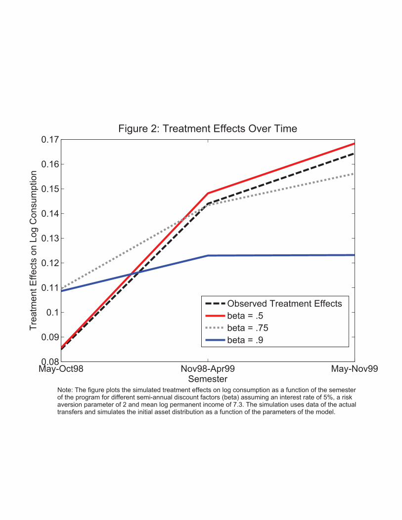
May-Oct98 Nov98-Apr99 May-Nov990.08

0.09

0.1

0.11

0.12

0.13

0.14

0.15

0.16

0.17Figure 2: Treatment Effects Over Time

Semester

Trea

tmen

t Effe

cts

on L

og C

onsu

mpt

ion

Observed Treatment Effectsbeta = .5beta = .75beta = .9

Note: The figure plots the simulated treatment effects on log consumption as a function of the semester of the program for different semi-annual discount factors (beta) assuming an interest rate of 5%, a risk aversion parameter of 2 and mean log permanent income of 7.3. The simulation uses data of the actual transfers and simulates the initial asset distribution as a function of the parameters of the model.

Control Treatment Control Treatment

May98-Oct98 - 386 - 392Nov98-Apr99 - 1,056 - 970May99-Oct99 - 1,305 - 1,147Nov99-Apr00 716 1,495 592 1,244May00-Oct00 1,415 1,682 1,140 1,355Nov00-Apr01 1,555 1,586 1,202 1,226May01-Oct01 1,820 1,870 1,381 1,419

Control Treatment Control Treatment

May98-Oct98 - 428 - 434Nov98-Apr99 - 1,147 - 1,054May99-Oct99 - 1,436 - 1,261Nov99-Apr00 718 1,605 593 1,335May00-Oct00 1,532 1,834 1,234 1,478Nov00-Apr01 1,719 1,793 1,329 1,386May01-Oct01 2,042 2,159 1,550 1,638

Note: The Unadjusted column shows average nominal transfers per household in pesos. The Adjusted column shows average real transfers per household deflated bimonthly to Sep/Oct 98 prices using national CPI. Panel A shows average transfers for the entire sample. Panel B shows average transfers for households that received transfers.

Appendix Table 1. TRANSFERS

Unadjusted Adjusted

Panel A. Average Transfers

Panel B. Average Positive Transfers

Unadjusted Adjusted

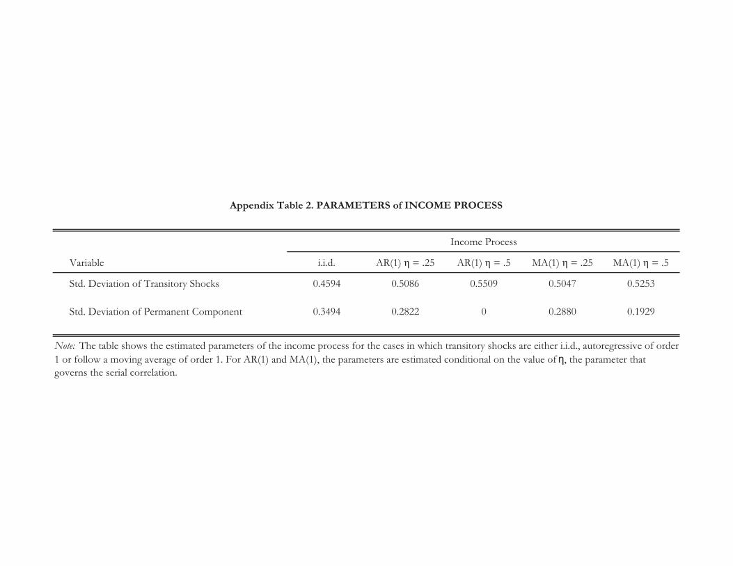
Variable i.i.d. AR(1) � = .25 AR(1) � = .5 MA(1) � = .25 MA(1) � = .5

Std. Deviation of Transitory Shocks 0.4594 0.5086 0.5509 0.5047 0.5253

Std. Deviation of Permanent Component 0.3494 0.2822 0 0.2880 0.1929

Appendix Table 2. PARAMETERS of INCOME PROCESS

Income Process

Note: The table shows the estimated parameters of the income process for the cases in which transitory shocks are either i.i.d., autoregressive of order 1 or follow a moving average of order 1. For AR(1) and MA(1), the parameters are estimated conditional on the value of �, the parameter that governs the serial correlation.

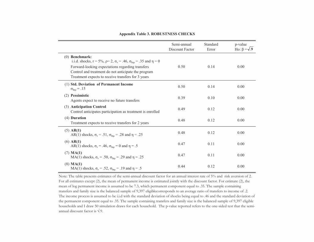
(0) Benchmark: i.i.d. shocks, r = 5%, �= 2, �� = .46, �ln� = .35 and � = 0Forward-looking expectations regarding transfersControl and treatment do not anticipate the programTreatment expects to receive transfers for 3 years

(1) Std. Deviation of Permanent Income�ln� = .15

(2) PessimisticAgents expect to receive no future transfers

(3) Anticipation ControlControl anticipates participation as treatment is enrolled

(4) DurationTreatment expects to receive transfers for 2 years

(5) AR(1)AR(1) shocks, �� = .51, �ln� = .28 and � = .25

0.49

Appendix Table 3. ROBUSTNESS CHECKS

Semi-annual Discount Factor

Standard Error

p-value Ho: � =

0.12 0.00

0.50 0.14 0.00

0.50 0.14 0.00

0.39 0.10 0.00

0.48 0.12 0.00

0.48 0.12 0.00

9.

(6) AR(1)AR(1) shocks, �� = .46, �ln� = 0 and � = .5

(7) MA(1)MA(1) shocks, �� = .50, �ln� = .29 and � = .25

(8) MA(1)MA(1) shocks, �� = .52, �ln� = .19 and � = .5 0.44 0.12 0.00

Note: The table presents estimates of the semi-annual discount factor for an annual interest rate of 5% and risk aversion of 2. For all estimates except (2), the mean of permanent income is estimated jointly with the discount factor. For estimate (2), the mean of log permanent income is assumed to be 7.3, which permanent component equal to .35. The sample containing transfers and family size is the balanced sample of 9,397 eligiblecorresponds to an average ratio of transfers to income of .2. The income process is assumed to be i.i.d with the standard deviation of shocks being equal to .46 and the standard deviation of the permanent component equal to .35. The sample containing transfers and family size is the balanced sample of 9,397 eligible households and I draw 50 simulation draws for each household. The p-value reported refers to the one-sided test that the semi-annual discount factor is �.9.

0.47 0.11 0.00

0.47 0.11 0.00

9.

0 0.5 1 1.5 20

5

x 104 beta = .5

0 0.5 1 1.5 202468

x 104 beta = .75

Freq

uenc

y

0 0.5 1 1.5 20

5

x 104 beta = .9

Assets / Permanent Income

Appendix Figure 1: Simulated Initial Asset Distribution

Note: The figure plots the simulated initial asset distribution for different semi-annual discount factors(beta) assuming an interest rate of 5% and a risk aversion parameter of 2.