NBER WORKING PAPER SERIES

GROWTH, URBANIZATION AND POVERTY REDUCTION IN INDIA

Gaurav DattMartin Ravallion

Rinku Murgai

Working Paper 21983http://www.nber.org/papers/w21983

NATIONAL BUREAU OF ECONOMIC RESEARCH1050 Massachusetts Avenue

Cambridge, MA 02138February 2016

For comments the authors thank Frederico Gil Sander and seminar participants at the University ofWaikato, New Zealand, and the World Resources Institute, Washington DC. These are the views ofthe authors and do not necessarily represent those of their employers, including the World Bank, anyof its member countries, or the National Bureau of Economic Research.

NBER working papers are circulated for discussion and comment purposes. They have not been peer-reviewed or been subject to the review by the NBER Board of Directors that accompanies officialNBER publications.

© 2016 by Gaurav Datt, Martin Ravallion, and Rinku Murgai. All rights reserved. Short sections oftext, not to exceed two paragraphs, may be quoted without explicit permission provided that full credit,including © notice, is given to the source.

Growth, Urbanization and Poverty Reduction in IndiaGaurav Datt, Martin Ravallion, and Rinku MurgaiNBER Working Paper No. 21983February 2016JEL No. I32,O15,O18,O47

ABSTRACT

Longstanding development issues are revisited in the light of our newly-constructed dataset of povertymeasures for India spanning 60 years, including 20 years since reforms began in earnest in 1991. Wefind a downward trend in poverty measures since 1970, with an acceleration post-1991, despite risinginequality. Faster poverty decline came with both higher growth and a more pro-poor pattern of growth.Post-1991 data suggest stronger inter-sectoral linkages: urban consumption growth brought gains tothe rural as well as the urban poor and the primary-secondary-tertiary composition of growth has ceasedto matter as all three sectors contributed to poverty reduction.

Gaurav DattDept. EconomicsMonash University (Clayton Campus)Melbourne, Australiagaurav.datt@monash.edu

Martin RavallionCenter for Economic ResearchGeorgetown UniversityICC 580Washington, DC 20057and NBERmr1185@georgetown.edu

Rinku MurgaiWorld BankLodi EstateNew DelhiIndiarmurgai@worldbank.org

2

1. Introduction

Past thinking about the impacts of economic growth on poverty in developing countries

has emphasized the role played by population urbanization.2 Building on classic papers by Lewis

(1954) and Kuznets (1955), a standard theoretical formulation of the migration process assumes

that distributions are preserved within both the rural and urban sectors.3 In essence, a

representative slice of the rural distribution is transformed into a representative slice of the urban

distribution in the process of people moving from rural to urban areas. The “Kuznets hypothesis”

implied by this model is often invoked in development policy discussions. A common view is

that the hypothesis justifies the expectation that growth will inevitably be inequality increasing in

poor countries, but that inequality will eventually start to decline.4 In theory, poverty measures

will, however, fall steadily under the Kuznets process as long as rural poverty measures exceed

urban measures (Anand and Kanbur, 1985).5 And the economy as a whole will grow as rural

residents take up the more lucrative urban jobs.

It is clear that within-sector distributional neutrality is a strong assumption. The

urbanization process in practice may well be quite selective, entailing significant distributional

shifts within one or both of the urban and rural sectors. For example, relatively less poor rural

workers may migrate, with gains, but be relatively poor in the destination urban sector; there is

evidence consistent with this pattern for the developing world (Ravallion et al., 2007). The

implications for inequality within each sector cannot be predicted easily.6

Even without population urbanization, within-sector growth processes are also relevant to

the overall outcomes for poverty. Various strands of the development literature have examined

these factors. One strand of the literature has questioned whether the agricultural growth

processes have helped the rural poor, many of whom are landless, while others have argued that

the benefits of rising farm productivity are passed on in due course through higher wage rates.7

2 Overviews of the literature can be found in Fields (1980) and Ravallion (2016). 3 As in Robinson (1976), Fields (1980) and Anand and Kanbur (1985, 1993). 4 The existence of such a turning point requires certain conditions to hold, which are specific to the measure of inequality used; Anand and Kanbur (1993) derive those conditions for various measures. 5 This holds for all population-weighted measures, such as all those characterized by Atkinson (1987). 6 This is known from research on the effects of selective compliance in household surveys on measures of inequality; see the analysis of this closely related issue in Korinek et al. (2006). 7 Contributions to this debate are cited in Ravallion and Datt (1996) and Datt and Ravallion (1998, 2011).

3

No less contentious is the role played by urban economic growth—whether it helps absorb

surplus rural labor and unemployed urban workers or merely benefits urban elites.8

Past research on these issues has relied mainly on cross-country comparisons, often in

single cross-sections (such as in the many tests of the Kuznets hypothesis) but sometimes using

panel data, though the typically short time-series has meant that the cross-country variability is

dominant. (While one can track economic growth annually for almost all countries, the

household surveys needed to monitor living standards are far less frequent.) In addressing these

issues, it is clearly desirable to have a reasonably long time series of surveys; a short series can

be deceptive for inferring a trend.

Amongst developing countries, India has the longest series of national household surveys

suitable for tracking living conditions. The surveys are reasonably comparable over time since

the basic survey instruments and methods have changed rather little (though we note, and

address, some comparability problems). India thus provides rich time series evidence—uniquely

so among developing countries—for testing and quantifying the relationship between living

standards of the poor and macroeconomic aggregates.

All the substantive issues about growth and poverty in the general development literature

have been prominent in the literature and policy debates on India. Famously, India's post-

independence planners hoped that the country's urban-based industrialization process would

bring longer-term gains to poor people, including through rural labor absorption.9 However, that

hope was largely shattered by the evidence of the slow pace of poverty reduction in the period

from Independence until the 1980s.10 In explaining this, a number of observers pointed to the

slow pace of labor absorption from agriculture associated with the more inward-looking and

capital-intensive development path of this period.11

The urban population share has been rising steadily over time in India, from 17% in 1950

to 31% today. However, India’s pace of population urbanization (proportionate increase in the

urban population share) has been less than either South Asia as a whole or lower middle-income

countries as a whole, and markedly slower than for (say) China.12 The trend rate of growth in

8 See, for example, the discussion in Eswaran and Kotwal (1994). 9 For a review of these debates see Ravallion (2016, Ch. 2). 10 See Datt and Ravallion (2002, 2011). 11 See, for example, Bhagwati (1993) and Eswaran and Kotwal (1994). 12 Urban population shares can be found in World Bank (2015 and past issues). The urban population shares of China and India were about the same around 1990, but the share now exceeds 50% in China.

4

India’s Net Domestic Product (NDP) per capita in the period 1958-1991 was under 2% per

annum, but it was more than double this rate in the period since 1992.13 The picture that emerges

from the accumulating evidence from India’s National Sample Surveys (that started in the 1950s)

indicates that economic growth in India had in fact been poverty reducing. Ravallion and Datt

(1996) showed that the elasticity of the incidence of poverty with respect to mean household

consumption was -1.3 over 1958-1991.14 Given the modest rate of growth over this period,

success at avoiding rising inequality prior to the 1990s was key to this finding.15

Many observers came to the view that too little growth was the reason for India’s slow

pace of poverty reduction. However, a deeper exploration of the data suggests that the sectoral

pattern of growth also played a role. Using data up to the early 1990s, Ravallion and Datt (1996)

found that rural economic growth was more poverty reducing, as was growth in the tertiary

(mainly services) and primary (mainly agriculture) sectors relative to the secondary (mainly

manufacturing and construction) sector. They also found that spillover effects across sectors

reinforced the importance of rural economic growth to national poverty reduction. Urban growth

and secondary sector growth had adverse distributional effects that mitigated the gains to the

urban poor, while urban growth brought little or no benefit to the rural poor. The slow progress

against poverty reflected both a lack of overall growth and a sectoral pattern of growth that did

not favor poor people.

There was much hope in India that the higher growth rates attained in the wake of the

economic reforms that started in earnest in the early 1990s would bring a faster pace of poverty

reduction.16 However, there have also been signs of rising inequality in the post-reform period,

raising doubts about how much the poor have shared in the gains from higher growth rates.17

The changes in India’s labor markets since around 2000 have potentially important

implications. There has been a tightening of rural casual labor markets, with rising real wage

13 NDP is gross domestic product less depreciation of capital. In order to better approximate incomes at the household level, we use net rather than gross product series in our analysis, though the two are highly correlated. Note that per capita incomes in the national accounts are also based on net product series. 14 They also found higher absolute elasticities for measures of the depth and severity of poverty, indicating that those well below the poverty line have benefited from economic growth, as well as those near the poverty line. 15 For evidence on this point for developing countries more generally see Bruno et al. (1998). 16 For an overview of India’s reform agenda since the early 1990s see Ahluwalia (2002) and Kotwal, Ramaswami and Wadhwa (2011). 17 Evidence of rising inequality in India since 1991 is reported in Ravallion (2000), Deaton and Drèze (2002), Sen and Himanshu (2004a,b) and Datt and Ravallion (2011).

5

rates, and also a narrowing of the urban-rural wage gap (Hnatkovska and Lahiri, 2013).18 Three

factors appear to be in play here. First, schooling has expanded, thus reducing the supply of

unskilled labor, especially in rural areas. Second, there has also been a decline in female labor-

force participation rates (Klasen and Pieters, 2015). Third, there has been a construction boom

across India, especially in (rural and urban) infrastructure, which had been neglected for a long

period. In 1993-94, the construction sector accounted for only 3.2% of employment for rural

males, but by 2011-12 this had risen to 13%.19 The shift of labor out of agriculture to the

nonfarm sectors has been more rapid since the 1990s.20 The shift has been to construction and

services, and also to manufacturing, to a smaller degree. Jacoby and Dasgupta (2015) suggest

that rising labor demand from construction has contributed to higher wages of unskilled labor

relative to skilled labor within rural areas, as well as rising rural relative to urban wages (for

male workers).

The combination of a lower supply of un-skilled labor and rising demand for that labor in

construction, transport and other services is likely to have been a driving force in higher casual

wages, in both farm and non-farm sectors and compressing the urban-rural wage gap. It is

unclear how permanent this change will prove to be. It may be conjectured that (like China)

India has reached its Lewis Turning Point. However, that is a conjecture, since there may well be

other factors leading to higher wages even while there is still rural underemployment. And

temporary reversals might be expected, notably if the current construction boom does not

continue.21

With the backdrop of this history of recent economic change in India, this paper revisits

the implications for poverty of both the higher rate of growth and the pattern of growth. The

sectoral imbalance in India’s post-reform growth would be a concern for poverty reduction if the

model linking poverty to growth had remained the same, notably with the rural and agricultural

sector contributing most to poverty reduction. However, previous research by Datt and Ravallion

(2011) found signs that the process of economic growth is changing in India, making urban

18 Hnatkovska and Lahiri (2013) also show that the narrowing of the wage gap persists when one controls for education and occupation. 19 These are our estimates based on the NSS 50th and 68th employment-unemployment survey rounds. 20 The share of agriculture, forestry and fishing in total (usual status) employment declined from 76% in 1993-94 to 49% in 2011-12 (Jacoby and Dasgupta, 2015). 21 At the time of writing (late 2015) lifted by public infrastructure investment, the construction sector has continued to expand overall, despite a slow-down in the residential building construction sector (Wilkes and Kumar, 2015). However, wage growth for construction workers has been lower than in other occupations.

6

economic growth more pro-poor in the post-reform period up to 2005-06. It is important to

know whether this pattern has continued in more recent data—to assess whether stronger

linkages from urban economic growth to rural poverty reduction have continued, alongside a

more economically diversified rural economy.

For the purpose of this paper we have compiled a new data series on poverty and related

data spanning 60 years, extending the period of analysis in past research.22 With the benefit of

nearly two decades of post-1991 data, we believe there is now sufficient data for the post-1991

period to test the poverty implications of the new rate and pattern of growth in post-reform India.

Attribution to reforms per se is problematic, but further scrutiny of the emergent properties of the

changing growth process with respect to poverty reduction is clearly important.

The sectoral structure of NDP growth in the post-1991 period is also of interest, as is the

role played by population urbanization, including the Kuznets process that has been so influential

in past thinking about the distributional implications of economic growth in poor countries.23 We

provide a decomposition of poverty reduction by sector of NDP and a decomposition method

that allows us to identify the difference between population urbanization effects with constant

within-sector distribution (as in the Kuznets process) versus changing within-sector distributions.

This enquiry delivers the most robust evidence to date that economic growth has not only

come with a lower incidence of absolute poverty in India but that there has been an acceleration

in the pace of progress against poverty in the post-1991 period. The new pattern of growth has

brought greater benefits to India’s poor. While there has been rising inequality within the rural

and (especially) urban sectors, growth within sectors has delivered sufficient gains to poor

people to assure falling poverty measures. Population urbanization played a role, but not in the

way assumed by the Kuznets process. Instead we find that urbanization came with distributional

changes within sectors; these were pro-poor in the pre-91 period, but that has not been so since

1991. Another difference is that the sectoral pattern of growth in NDP mattered less to progress

against poverty post-1991 than was the case in the pre-1991 period.

22 The period of analysis in Ravallion and Datt (1996) ended at about the time (1991) when India’s process of economic reform started in earnest. Datt and Ravallion (2011) updated Ravallion and Datt (1996) by incorporating an extra 14 rounds of the National Sample Surveys (NSS) taking the series up to 2006. This paper extends the series to 2012. 23 Datt and Ravallion (2011) did not study the sectoral structure of NDP or identify the role played by the Kuznets process.

7

The following section describes the data set we have created for this task. Section 3

provides some key summary statistics, and section 4 investigates the relationship between

poverty and overall economic growth. Section 5 studies the poverty impact of urban-rural

composition of growth in mean consumption, while Section 6 turns to the sectoral composition

of growth in net domestic product. A key focus in sections 3-6 is on changing patterns across the

pre-reform and post-reform periods. Section 7 concludes.

2. Data

For the purpose of this study, we have derived a new and consistent time series of

poverty measures for rural and urban India over the period 1951 to 2012. This is based on

consumption distributions from 51 household surveys conducted by the National Sample Survey

Organization (NSSO); beginning with the 3rd round for August-November 1951 up to the 68th

round for July 2011 to June 2012. We use the full period for descriptive purposes. Some of the

earliest surveys had smaller sample sizes and covered shorter periods. The shorter periods also

make for a more imprecise mapping between NSS rounds and the annual national accounts data.

Hence, in our main analysis we dropped some of the early NSS rounds that had survey periods

considerably shorter than a year, and our first observation for the poverty regressions in this

paper is for the 13th round for 1957-58.24 For the econometric analysis we restrict ourselves to

the period 1957-2012 (from NSS round 11 to round 68), giving 41 observations including 18 for

the post-1991 period.25 This series significantly improves upon the most widely-used time series

on poverty measures in India to date.

Following now well-established practice for India and elsewhere, a household's standard

of living is measured by real consumption expenditure per person. The underlying NSS data do

not include incomes, though it can be argued that current consumption is a better indicator of

living standards than current income.26 Nonetheless, there are various “non-income” dimensions

24 Data from the earlier rounds are included in the graphs, though poverty measures for rounds 4 and 5, rounds 6 and 7, rounds 9 and 10 and rounds 11 and 12 are aggregated as survey-period-weighted averages. Thus, for instance, the headcount measure for combined rounds 11 (for August 1956-February 1957) and 12 (for March-August 1957) is 7/13-th of the headcount index for round 11 plus 6/13-th of the headcount index for round 11. 25 Most of our regressions for changes in poverty are based on 40 observations; they exclude the 48th round for 1992, the year of the macroeconomic crisis that provided an impetus for economic reforms. Thus, effectively, the change in poverty between the 47th round (for July-December 1991) and 48th round is not included in either the pre-1991 or the post-1991 period. 26 For an overview of these arguments see Ravallion (2016, Chapter 3).

8

of well-being that this measure cannot hope to capture, and we say nothing here about how

responsive these other dimensions may be to growth.

While the NSS surveys are highly comparable over time by international standards, there

is a comparability problem in the rounds since the early 1990s. While most of the surveys have

used a uniform recall period of 30 days for all consumption items, seven of the survey rounds in

the post-91 period have instead used a mixed-recall period (MRP), with longer (one year) recall

for some (mainly non-food) items.27 On a preliminary investigation of the data we found that the

use of a mixed recall period increased the mean and reduced inequality, implying lower poverty

measures. All our regressions below include a control for MRP survey rounds.

Poverty lines and price indices: We report results for two poverty lines. Following Datt

and Ravallion (2011), one line is that originally defined by the Planning Commission (1979), and

endorsed by Planning Commission (1993). This poverty line is anchored on a nutritional norm of

2400 calories per person per day in rural areas and 2100 calories for urban areas, and

corresponds to a per capita monthly expenditure of Rs. 617 and Rs. 922 (rounded to the nearest

rupee) in rural and urban areas respectively at 2011-12 prices.28 The second poverty line

corresponds to the rupee value of the international poverty line of $1.25 per person per day at

2005 PPP dollars, and are equivalent to rural and urban per capita monthly expenditures of Rs.

732 and Rs. 1115 at 2011-12 prices.29 The second set of lines are thus about 20% higher than the

first set of lines.

The nominal values of the poverty lines for different NSS rounds are evaluated using

separate urban and rural price indices. Our price indices are mainly based on the all-India

Consumer Price Index for Industrial Workers (CPIIW) as the deflator for the urban sector, and

the all-India Consumer Price Index for Agricultural Laborers (CPIAL) as the deflator for the

rural sector. However, our final price indices also incorporate some adjustments aimed at

constructing a consistent time series over the long period of analysis; these adjustments relate to 27 In particular, one-year reference is used for clothing, bedding, footwear, education, medical (institutional) and durable goods. Mixed reference periods have been used for seven NSS rounds in our data, viz., rounds 55, 56, 57, 58, 59, 60 and 62. 28 The original Planning Commission lines correspond to rural and urban per capita monthly expenditures of Rs. 49 and Rs. 57 at 1973-74 prices. At 2005 purchasing power parity (PPP), these lines have a value of $1.03 per day in 2005. See Ravallion (2008) for further discussion, including comparisons with a higher international poverty line. 29 Neither set of lines is directly comparable to India’s current official “Tendulkar” poverty lines. At 2005 PPP, the

Tendulkar lines have a value of $1.17 per day in 2005, incorporating a lower cost of living differential rural and urban areas than the original Planning Commission lines on which our poverty line series is based. The Tendulkar poverty lines are only available after 1993-94.

9

the use of the Consumer Price Index for the Working Class for the period before August 1968 for

which the CPIIW did not exist, a correction for the constant price of firewood for a part of the

Labour Bureau’s CPIAL series, and the use of a reweighted chain price index in both rural and

urban areas to better approximate the weight of food in the consumption basket of the poor.30

Our final rural and urban price indices are averages of monthly indices corresponding to the

exact survey period of each NSS round.

Poverty measures: We use three poverty measures: the headcount index (H), given by the

percentage of the population living in households with a consumption per capita less than the

poverty line; the poverty gap index (PG), defined by the mean distance below the poverty line

expressed as a proportion of that line, where the mean is formed over the entire population,

counting the non-poor as having zero poverty gap; and the squared poverty gap index (SPG),

defined similarly to PG except that it is the mean of the squared proportionate poverty gaps.

Unlike PG, SPG is sensitive to distribution amongst the poor, in that it satisfies the transfer

axiom for poverty measurement.31 In particular, to economize space we report results on H, PG

and SPG for the higher line, and only H for the lower line.

The overall level of poverty at date t can be additively decomposed using population

weights. We will be interested in the urban-rural decomposition of the aggregate measure for

date t:

rtrtututt PnPn= P + (t=1,..,T) (1)

where itn and itP are the population shares and poverty measures for sectors r u, =i for urban

and rural areas respectively. “Time” (t) represents the ordering of the T survey rounds in time,

which can differ from real time given the uneven spacing. 32

Demographic data: The population estimates are based on the Census population totals

and assume constant growth rates for urban and rural populations between censuses. We use the

NSSO’s urban-rural classification.33 Over such a long period, some rural areas would have

become urban areas. To the extent that rural (non-farm) economic growth may help create such

30 See Datt and Ravallion (2011) for further details on these adjustments. 31 All three measures are members of the class of measures proposed by Foster, Greer and Thorbecke (1984). 32 Controlling for unequal time interval between survey rounds made little difference to the results. 33 The NSS follows the Census definition of urban areas which includes all places with a municipality, corporation, cantonment board or notified town area committee, and places that meet a number of criteria including a population greater than 5000, a density not less than 400 persons per sq. km. and three-fourths of the male workers engaged in non-agricultural pursuits. In the 2011 Census, 31.2% of the total population was classified as urban.

10

re-classifications, as successful villages evolve into towns, this process may produce a downward

bias in our estimates of the (absolute) elasticities of rural poverty to rural economic growth. The

impact on the urban elasticities could go either way, depending on the circumstances of new

urban areas relative to the old ones. We have no choice but to use the NSSO/Census

classification. The rural and urban population estimates are also centered at the mid-points of the

NSSO’s survey periods.

National accounts: We use private final consumption expenditure and net domestic

product and its sectoral components from the National Accounts Statistics (NAS). To mesh the

NAS data with the poverty data from the NSSO, we have linearly interpolated the annual

national accounts data to the mid-point of the survey period for different rounds.

There has been a rising gap over time between NAS and NSS consumption aggregates.34

From the point of view of the present discussion, it is notable that the NSS series does not fully

reflect the large gains in mean consumption indicated by the NAS from the early 1990s onwards.

The ratio of NSS-to-NAS consumption declined from about 70% in 1957 to 60% in 1991, and

then steeply to 39% in 2011-12.

We do not know how much of the gap is due to errors in NAS consumption versus NSS

survey methods. Until recently, the NSSO’s methods appear to have changed rather little over

many decades. That is probably good news for comparability reasons, although it does raise

questions about whether their methods are in accord with international best practice. However, it

is notable that the MRP rounds of the NSS have helped close the gap between the NAS and NSS

consumption aggregates.35 Regressing the log difference of the NSS mean ( tµln∆ ) on the log

difference of NAS consumption per capita ( tCln∆ ) and the change in the dummy variable for

MRP rounds, we get:

ttt MRPC= ∆+∆∆)021.0()141.0(

067.0ln692.0ln µ

The positive and significant coefficient for MRP suggests that NSS design may account for at

least some of the discrepancy between the two data sources.

34 The gap is not only found in India, but it is larger there than most other countries (Ravallion, 2003). 35 The MMRP (modified-mixed reference period) aggregate introduced in the 2009-10 and 2011-12 rounds has further closed the gap. The MMRP method which reduces the recall period for some food items to a 7-day recall (compared to a 30-day recall in the MRP) brings NSSO’s practices closer to the more common practice of a two week or less recall period for food items in other countries.

11

However, it is also important to note that the gap between the consumption aggregates

from these two sources does not necessarily imply that the NSS overestimates poverty. Some of

the gap is due to errors in NAS consumption, which is determined residually in India, after

subtracting other components of domestic absorption from output at the commodity level. There

are also differences in the definition of consumption, and there are things included in NAS

consumption that one would not use in measuring household living standards.36 Some degree of

under-reporting of consumption by respondents, or selective compliance with the NSS’s

randomized assignments, is inevitable. However, it is expected that this is more of a problem for

estimating the levels of living of the rich than of the poor.37 We will look into the implications of

the growing drift between NAS and NSS consumption in regressions that use (sectoral) growth

variables from the NAS.

3. Summary statistics

India’s urban population share has risen steadily over the 60 years, at about 1% per

annum (0.25 percentage points per annum) over the 60-year period; Figure 1 plots the urban

population share. (The extent of the linearity is possibly deceptive given that interpolations are

used between census years, as noted in Section 2.)

As can also be seen from Figure 1, poverty incidence showed no significant trend up to

about 1970, but fell after that. (The series for the two poverty lines track each other closely.)

Both higher growth rates and a higher pace of poverty reduction are evident in the post-1991

period; Table 1 provides the trend rates of growth.

Much of the faster growth post-1991 has occurred in the “tertiary” sector of India’s

economy, which is primarily services and trade. The growth rate of tertiary sector NDP per

capita doubled in the post-1991 period (after 1992), from 3.1% per annum up to 1991 to 6.4%.38

The secondary sector also picked up, from 2.9% per annum to 4.5%.39 So too did the primary

sector, but at a much lower level; the pre-1991 growth rate in primary NDP per capita was only

36 For further discussion of the differences between the two data sources see Sundaram and Tendulkar (2001), Ravallion (2000, 2003), Sen (2005) and Deaton (2005). 37 There is evidence from other sources consistent with that expectation; see Banerjee and Piketty (2003) on income under-reporting by India’s rich. 38 These are OLS regression coefficients on time; the standard errors are 0.04% and 0.2% respectively. 39 The standard errors are 0.1% and 0.3% respectively.

12

0.2% per annum, while it rose to 0.8% in the post-1991 period.40 As one would expect, the share

of the primary sector in NDP has fallen appreciably from 55% in the early 1950s to 15% in 2012.

The acceleration in survey-based mean real consumption growth—from 0.6% per annum

in the pre-1991 period to 2.0% in the post-1991 period—is significant. The urban and rural

trends reveal a pattern that is similar to the national level, though there are some differences

between the two segments of the economy (Table 2). The NSS mean consumption growth rates

are appreciably higher (nearly twice as high) post-1991 in both rural and urban areas.

Faster growth post-1991 has also come with rising inequality within urban areas, but less

so in rural areas. Figure 2 plots the indices over time. Note that these are the “raw” values,

without adjustment for the effect of MRP rounds. When we add controls for MRP rounds, we

also see rising inequality in rural areas post-1991. Table 2 gives the exponential trends for the

Gini index. In contrast to a declining trend in rural Gini and no trend in urban Gini in the pre-

1991 period, a significant positive trend in inequality emerged post-1991 in both sectors. The rise

in inequality has been greater in urban areas. At the same time, inter-sectoral inequality has been

generally rising. We see from Figure 3 that the ratio of urban mean to the rural mean has been

rising since around 1970 (the early observations were volatile, and should probably be

discounted), though with signs of levelling off and even decline since 2000. Controlling for MRP

rounds, time trends in the ratio of real urban-to-rural mean consumption are similar pre- and

post-91, with the ratio increasing at about 0.14% per annum in both periods. So the higher

growth in the post-1991 period has come with generally rising consumption inequality,

especially within sectors, but also to some extent between them.

Datt and Ravallion (2011) also found higher trend rates of poverty reduction in the post-

1991 period, but the differences (compared to the pre-1991 period) were only statistically

significant for the headcount index (nationally and for urban areas). Our new series provides a

more statistically robust indication of acceleration in progress against poverty post-1991 for both

poverty lines (Table 1). Over the 55-year period, the exponential trend decline (for the higher

line) was 1.3% per annum for the headcount index, rising to 2.3% and 3.0% for the poverty gap

index and squared poverty gap index respectively.41 For the period prior to 1991, the trends were

0.6%, 1.4% and 2.0% for H, PG and SPG, while the corresponding post-1991 trends were 3.6%, 40 The standard errors are 0.05% and 0.2% respectively. 41 Similarly to the NDP growth rates reported in the introduction, the growth rates were estimated as parameters of a single regression, constrained to assure that the predicted values were equal in 1992.

13

5.2% and 6.3%. The differences between the pre- and post-1991 trends are statistically

significant (Table 1). We also find a faster pace of poverty decline post-1991 in both rural and

urban areas, and this is significant for all three measures (Table 2). Figure 4 plots the headcount

indices for the lower line; the pattern over time is similar for the higher line and other measures.

Alternatively one can define the trend in the level of the poverty measure rather than its

log. This again confirms the finding of an acceleration in the post-1991 period of both growth

and poverty reduction as measured by H and PG (though not SPG). In other words, the post-1991

period has witnessed larger annual percentage point reductions in the incidence and depth of

poverty while the annual percentage point reduction in the severity of poverty has remained

about the same. As noted above, all poverty measures for both sets of poverty lines exhibit larger

proportionate reductions in the post-1991 period.

Historically, poverty measures have been higher for rural India. However, as can be seen

from Figure 4 that there has been a marked convergence of poverty measures between urban and

rural areas. Figure 5 plots the difference between the rural and urban headcount indices for both

poverty lines. Intuitively, since growth rates in mean consumption were slightly higher in urban

areas, the poverty convergence between urban and rural areas is a distributional effect, stemming

in part from the fact that inequality has risen more within urban areas and part from the fact that

inequality was initially lower in rural areas, making growth more poverty reducing (Ravallion,

2007). Thus rural growth has had greater impact on rural poverty than for urban areas.

The convergence process started around 1980, but has been noticeably more rapid since

2000. This is consistent with related evidence on the narrowing urban-rural wage gap

(Hnatkovska and Lahiri, 2013). Going forward, one implication of this sectoral poverty

convergence is that the Kuznets process will contribute little to overall poverty reduction, and

may even be poverty increasing. The next section will look more deeply into the urban-rural

pattern of growth and poverty reduction, including the role played by the Kuznets process.

A further implication of these findings is that there has been a marked urbanization of

poverty in India. Figure 6 gives the proportion of the poor living in urban areas over time for

both poverty lines. In the early 1950s, 14% of the poor lived in urban areas; by 2012 this had

risen to 35% for the lower line and 32% for the upper line. This is broadly consistent with the

pattern found in other developing countries (Ravallion et al., 2007). There is a sign of

acceleration in the pace of the urbanization of poverty since 2000.

14

4. Poverty and overall economic growth

Any poverty measure found in practice can be written as a function of the survey mean

relative to the poverty line and the relative distribution of income, as represented by the Lorenz

curve.42 When the poverty line is fixed in real terms, all such poverty measures are strictly

decreasing functions of the mean ( tµ ) for any given relative distribution (though the elasticity

can vary greatly, depending on the initial mean and Lorenz curve). A higher growth rate may

also entail a shift in distribution for or against the poor. In characterizing the overall poverty

impact of growth, we are interested in the total effect of growth on poverty, allowing distribution

to change, rather than the partial effect, holding distribution constant.43 We call this the “growth

elasticity of poverty reduction”, or “growth elasticity” for short.

We estimate the growth elasticities at the national level by the regression coefficient of

log poverty measure ( tPln ) on log mean per capita consumption ( tµln ) across the available time

series, allowing the error term to be autocorrelated and heteroskedastic. Whenever both the

dependent and independent variable of such a regression are estimated from the same survey data

the possibility arises of bias due to the fact that measurement errors in the survey can be passed

onto both variables; when overestimating the mean, for instance, one will tend to underestimate

poverty. (The sign of the bias is theoretically ambiguous since measurement error in the

independent variable will also induce an attenuation bias in the least squares estimate of the

elasticity.) We also provide an Instrumental Variables (IV) estimator, in which the instruments

excluded any variables derived from the same survey as the dependent variable. Our estimates

also control for the use of mixed reference periods for some of the NSS rounds.

Table 3 gives our estimates of the elasticities of all three poverty measures with respect to

three measures of economic growth based on: (i) consumption per person from the NSS; (ii)

consumption per person as estimated by the NAS and population census; and (iii) NDP

("income" for short) per person, also from the NAS and census. In all cases, the elasticities are

estimated by regressing the log poverty measure on the log mean consumption or income. We

also give an "adjusted" estimate in which a control variable was added for the first difference of

42 This follows from the fact that the mean and the Lorenz curve fully specify the cumulative distribution function. 43 Analytic formulae for the partial elasticities are found in Kakwani (1993). On the conceptual distinction between the partial and total elasticities in this context, see Ravallion (2007).

15

the log of the ratio of the consumer price index to the national income deflator (i.e., the

difference in the rate of inflation implied by the two deflators).44 This was included to allow for

possible bias in estimating the growth elasticity due to the difference in the deflator used for the

national accounts data and that used for the poverty lines.

For the 1957-2012 period as a whole, the national poverty measures responded

significantly to growth in all three measures. The IV estimates to address survey measurement

errors (also likely to be negatively correlated between the dependent variable and the explanatory

variable) are slightly lower than the corresponding OLS estimates. The (absolute) elasticities are

higher if one uses the NSS estimate of mean consumption, rather than the national accounts

estimate. The elasticities are lowest for per capita income. There are a few possible reasons.

Inter-temporal consumption smoothing may make poverty (in terms of consumption) less

responsive in the short-term to income growth than to consumption growth. Imperfect matching

of the time periods between the NSS and the NAS could also be playing a role in attenuating the

elasticities using NAS growth rates. A further reason for lower (absolute) elasticities with respect

to NAS consumption or income has to do with the increasing divergence between NSS and NAS

growth rates of mean consumption; significantly faster growth in NAS means relative to NSS

means is reflected in the lower elasticities with respect to the former.

When we split the period into two at 1991, we find appreciably higher (absolute)

elasticities of poverty indices with respect to the survey mean in the post-1991 period; the

difference in the estimated elasticities over the two periods is statistically significant.45 The

pattern of higher post-1991 elasticities is similar for all poverty measures, for higher and lower

poverty lines and for the OLS as well as the IV estimates (Table 3).

By comparison, we find that NAS-based growth of both income and consumption per

capita indicate significantly higher (absolute) elasticities in the post-1991 period for the

headcount index, but the difference between the two periods is not statistically significant for

SPG, and for PG it is significant only for the per capita income growth elasticity. It is

nevertheless notable how much difference there is in the elasticity based on the NSS

44 The consumer price index is a consumption share-weighted average of the rural and urban price indices. 45 See Table 3. These results are based on regressions of log poverty measures on log survey mean interacted with dummy variables for pre- and post-1991 periods, and a dummy variable for MRP surveys. The regressions also incorporate a kink at NSS round 47 (July-December 1991) such that there is no discontinuity in the predicted values of log poverty measures between the pre- and post-1991 periods.

16

consumption growth rates versus the NAS growth rates for the post-1991 period; the survey-

based elasticities are about twice as high (in absolute terms) as the national accounts based

elasticities. The much lower NAS elasticities reflect the NAS-NSS drift (much faster NAS-

based growth relative to that based on the NSS) post-91.

Our results are qualitatively robust to the choice of poverty measure. However, it is

notable that the growth elasticities tend to be highest (in absolute value) for SPG and higher for

PG than H. The higher growth elasticity of PG than H implies that the depth of poverty (as

measured by the mean poverty gap relative to the poverty line) is also reduced by growth.

Similarly, the even higher elasticity of SPG implies that inequality amongst the poor (as measured

by the squared coefficient of variation) is reduced by growth. Thus the impacts of growth within

and between sectors are not confined to households in a neighborhood of the poverty line.

To summarize: The responsiveness of poverty to growth when measured from the surveys

is generally greater in the post-1991 period. This is also true of the responsiveness of the headcount

index to growth measured using the national accounts, but not for the two poverty gap indices (PG

and SPG), which are similarly responsive to growth in the two periods.

5. Poverty and the urban-rural pattern of growth

Our proposed test for whether the sectoral composition of growth matters entails

estimating the following regression equation on the discrete time-series data on poverty and

growth:

)2(ln)/(

lnlnln

1111

11

T,..,=t + n nn s- s

+ s + s = P

trtutrtutrtn

rtrtrututut

επ

µπµπµµ

µµ

∆

∆∆∆

−−−−

−− (2)

Here ∆ is the discrete-time difference operator (such that 1−−≡∆ ttt xxx ), tititit /n= s µµµ is sector

i’s share of mean consumption at survey round t and µ it is the mean consumption for sector i .

The π 's are parameters to be estimated. To motivate this test regression, notice that, under the null

hypothesis that ππππ =nru ++ , equation (2) collapses to:

ttt + = P εµπ lnln ∆∆ (3)

Thus, under this null, it is the overall rate of growth that matters, not its composition. By testing

that null we determine whether the composition of growth matters. If this null is rejected then the

17

pattern of growth matters and the ru ππ , parameters can be interpreted as the impact of (share-

weighted) growth in the urban and rural sectors respectively, while π n gives the effect of the

population shift from rural to urban areas.

We also test whether economic growth in one sector has cross-effects on distribution in

the other sectors. Here we can decompose (2) for the rate of growth in average poverty into

three components:

utrtutrtutrtunrtrturututuuut

P

ut + n nnss+ s + s= Ps επµπµπ µµµµ ln)/(lnlnln 1111111 ∆−∆∆∆ −−−−−−− (4.1)

rtrtutrtutrtrnrtrtrrututrurt

P

rt + n nnss+ s + s= Ps επµπµπ µµµµ ln)/(lnlnln 1111111 ∆−∆∆∆ −−−−−−− (4.2)

nrtutrtutrtnn

rtrtnrututnurtutrt

P

ut

P

rt

+nnnss

+ s s =n nnss

επ

µπµπµµ

µµ

ln)/(

lnlnln)/(

1111

111111

∆−

∆+∆∆−

−−−−

−−−−−− (4.3)

where titit

P

it /PPn= s for r u, =i , and njrjujj ππππ ++= for nr u, =j , . So summing (4.1), (4.2)

and (4.3) yields (2). By interpretation, (4.1) shows how the composition of growth and population

shifts impact on urban poverty; (4.2) shows how they impact on rural poverty; and (4.3) gives the

impact on the population shift component of Plog∆ . We estimate (4.1) and (4.2); (4.3) need not

be estimated separately since its parameters can be inferred from the estimates of (4.1) and (4.2)

using the adding-up restriction. As before, since our main interest is in a comparison of the pre-

and post-reform periods, we allow the π parameters to differ across the two periods.

Table 4 presents our estimates of equations (2), (4.1) and (4.2), summarizing the poverty

impact of the urban-rural composition of consumption growth. Table 5 gives the test statistics on

whether the urban-rural composition of growth matters and whether the population shift effect is

significant. Table 6 reports elasticities of poverty with respect to rural and urban growth. These

results are presented for national poverty measures as well as separately for urban and rural

areas, and for the two poverty lines.

The first point to note from Table 4 is that there is a significant structural break at 1991.

The pre-91 and post-91 model parameters are significantly different from each other; the null of

parameter equality is rejected in almost all cases in Table 4. Beginning with results at the

national level, for the pre-1991 period we confirm the earlier finding of Ravallion and Datt

(1996) that the growth effects on poverty for the pre-1991 period are largely attributable to rural

18

consumption growth, with virtually no contribution from urban growth, while the population

urbanization process also contributes to poverty reduction.

We are also able to confirm the earlier finding of Datt and Ravallion (2011) that with the

post-reform structural break this pattern has changed substantially. In the post-1991 period, while

rural growth remains significant for poverty reduction, unlike the pre-1991 period, it is no longer

the prime driver of national poverty reduction. The most notable change is that urban growth

now has a significant impact on poverty. Thus, with additional recent data and also for a higher

poverty line, we are able to confirm the emergence of a significant effect of urban consumption

growth on national poverty as a striking feature of the post-1991 pattern of economic growth in

India.

Also notable is the change in the sign of the population shift effect from being poverty-

reducing in the pre-91 period to becoming poverty-increasing post-91. As this effect is estimated

conditional on urban and rural mean consumption growth, it can be interpreted as picking up

intra-sectoral distributional effects associated with the shift of population from rural to urban

areas. The changing sign of this effect post-91 is indicative of the adverse distributional changes

that have accompanied faster post-reform growth.

The last four columns of Table 4 help unpack these shifting patterns observed for national

poverty measures by urban and rural areas. In qualitative terms, there is not much change

between the pre- and post-91 periods in how urban and rural growth appear to have affected

urban poverty, which was highly responsive to urban consumption growth in both periods, and

generally unresponsive to rural growth except for the PG and SPG measures in the pre-91 period.

The main change across the two periods with regard to urban poverty is quantitative; the

marginal effects of urban growth on urban poverty are much larger post-91.

By comparison, there are important changes for rural poverty in both qualitative and

quantitative terms. The most notable change is that while in the pre-91 period urban growth had

no discernible impact on rural poverty, a significant and large impact emerged post-91. Rural

growth has continued to be important for rural poverty reduction.

Taken together, these results suggest that the post-reform importance of urban growth for

national poverty reduction is driven by urban poverty becoming more responsive to urban

growth and even more importantly by the emergent and quantitatively substantial response of

rural poverty to urban growth.

19

In light of the differential though changing effects of rural-urban growth and population

urbanization, it is not surprising that the hypothesis that the rural-urban composition of growth

does not matter for poverty reduction is rejected in most cases (Table 5). For urban poverty, it is

rejected strongly in virtually every case.

Note that the estimates in Table 4 relate to the poverty effects of share-weighted urban

and rural growth. In the estimation framework of equations (2), (4.1) and (4.2), the elasticities of

poverty with respect to urban and rural growth are in fact not constant. They depend on the

shares of urban and rural sectors in national consumption and national poverty. Table 6 reports

these elasticities at mean shares for the pre-91 and post-91 periods. The contrast for the two

periods for national poverty measures is notable. There is a reversal in the relative magnitudes of

urban and rural growth elasticities. From being lower in absolute terms than elasticities for rural

growth in the pre-91 period, the urban growth elasticities are higher post-91, despite the still

smaller share of the urban sector in national consumption and national poverty. Indeed, with the

exception of the headcount index at the higher poverty line, the elasticities of rural poverty

measures with respect to urban growth are even higher than those with respect to rural growth.

A unified decomposition: The marginal effects of share-weighted growth or the growth

elasticities do not by themselves tell us about the relative contributions of different components of

growth and population urbanization to observed poverty reduction over the pre- and post-reform

periods. To assess this, we now combine analytic and regression-based decomposition methods to

provide a further insight into the changing sources of poverty reduction.

A starting point is to note that the population urbanization effect in equations (2) and (4)

pertains to a fixed mean within each sector. In the development literature the Kuznets effect refers

to the impact on overall inequality of population urbanization holding the levels distribution (and

hence poverty levels) constant within both the urban and rural sectors.46 Thus the population

urbanization effect in (2) and (4.1) combines the “Kuznets effect” of urbanization processes with

within-sector distributional changes associated with urbanization. We now separate the two—to

see how much the pure Kuznets effect has contributed to poverty reduction in India, and its

importance relative to intra-sectoral distributional changes as well as intra-sectoral growth. This

46 This is in keeping with the argument of Kuznets (1955) and subsequent formalizations by Robinson (1976), Fields (1980)and (for a more general class of inequality measures) Anand and Kanbur (1993).

20

requires a unified decomposition, combining the analytic and regression-based decompositions

as developed below.

Returning to equation (1) and taking the differential, the analytic (exact) decomposition

of the change in the poverty measure can be written as:

utut

P

utrtrt

P

rt

ut

P

utrt

P

rtut

P

utrt

P

rtt

nPsnPs

nsnsPsPsP

lnlnlnln

lnlnlnlnln

11

1111

∆∆+∆∆+

∆+∆+∆+∆=∆

−−

−−−− (5)

where the first two terms refer to the contribution of within-sector poverty change, the third and

the fourth to the contribution of population shift (urbanization), and the last two to the

contribution of the interaction between sectoral poverty change and population shift. Note that

the first two terms are already estimated in regressions (4.1) and (4.2), which can be embedded

in (5).

Next, consistently with the idea of the Kuznets effect, imagine holding the poverty

measures constant in both urban and rural areas while allowing for urbanization. This gives the

Kuznets effect:

rtutrt

P

ut

P

rtut

P

utrt

P

rtPPtt nnnssnsnsP Kru

ln)/(lnln)ln( 1111110 ∆−=∆+∆=∆≡ −−−−−−=∆=∆ (6)

Thus, the Kuznets effect is the same as the third and fourth terms in equation (5). Of course,

population urbanization can also entail distributional changes within each sector, but these effects

are already reflected in the population shift terms in equations (4.1) and (4.2). Collecting these

terms, we can also define the following population effect controlling for the means within each

sector and thus representing intra-sectoral distributional change:

rtutrtutrtrnutrtutrtunt n nnssnnssN ln)]/()/([ 11111111 ∆−+−≡ −−−−−−−−µµµµ ππ (7)

Equations (4.1) and (4.2) allow us to specify the effects of growth in mean consumption in the

two sectors as:

µππ µµrtrtrrrtur

r

t s + s G ln)( 11 ∆≡ −− (8.1)

s sGututruutuu

u

t µππ µµ ln)( 11 ∆+≡ −− (8.2)

Substituting into (5), the expected change in the (log) poverty measure (forming the expectation

over the distribution of the error terms in (4.1) and (4.2)) is then given by:

ttt

u

t

r

tt IKNGGPE ++++=∆ )ln( (9)

where

21

utut

P

utrtrt

P

rtt nPsnPsI lnlnlnln 11 ∆∆+∆∆= −− (10)

is the interaction effect between changes in poverty and changes in population shares within each

sector.

In summary, the total change in the poverty measure can be decomposed into four terms:

i) rG and u

G are the effects of rural and urban growth in mean consumption.

ii) N is the effect of population shift, as from the regression model, controlling for

growth in mean consumption within each of the urban and rural sectors. Thus this

term picks up any within-sector distributional effects of population urbanization.

iii) K is the classic Kuznets effect of population shift holding within-sector poverty levels

constant.

iv) I is the interaction effects between sectoral poverty change and population shift.

As noted in the introduction, while the Kuznets effect is poverty decreasing, when

distributions shift within sectors, the overall impact on any standard measure of poverty,

controlling for the change in the mean, is theoretically ambiguous. The outcome depends, in

part, on which segments of the rural distribution become urban, and where they end up in the

urban distribution. However, even in simple cases, such as when it is the rural non-poor who

move to urban areas, the inequality impacts are theoretically ambiguous (Korinek et al., 2006).

The four components in (9) can be readily computed for the pre- and post-1991 periods

from the foregoing analysis. Thus, the annual rate of poverty reduction and its components for

the pre- (post-) reform period are obtained by summing up equation (5) over the pre- (post-)

reform period and dividing by the length of the pre- (post-) reform period. Components K and I

are directly computed as the last four terms in equation (5), while Gr, Gu and N are evaluated

from the estimates of regressions (4.1) and (4.2) discussed earlier.

Table 7 presents the results of this unified decomposition. In the pre-1991 period, almost

all the reduction in poverty comes from two sources: growth in rural mean consumption (45-

46%) and population urbanization component (N), allowing distributions to change within

sectors (48-52%). The Kuznets effect accounts for 3% or less of the overall reduction in the

poverty, while urban growth contributes 6% or less (1% or less for the reduction in headcount

index). In sharp contrast, during the post-1991 period, urban growth has played a much more

important role (accounting for 63-84% of the decline in the national poverty), while rural growth

22

has continued to be important (accounting for 47-70%). Against these effects, there was a

poverty increasing intra-sectoral distributional change (increasing the poverty measures by 23-

33% of the overall change), while the Kuznets effect was even less quantitatively important.

6. Poverty and the sectoral structure of net domestic product

It is also of interest to know how the relationship between poverty and the sectoral

structure of national output has evolved over time. By decomposing the overall growth rate of

net domestic product (NDP) into its components we can investigate how the composition of NDP

growth has mattered to poverty reduction. The national accounts do not of course have an

“urban-rural” breakdown, so this dimension is now latent.

We divide NDP per capita, ty , into k sources as ∑=

=k

i

itt yy1

. Taking the differences over

time, we can write the growth rate of NDP as the share-weighted sum of the growth rates across

the k sources, i.e., ∑=

− ∆=∆k

i

ititt ysy1

1 lnln where titit yys /= is the share of NDP due to the i’th

source. (This uses the approximation that ttt yyy ln/ 1 ∆≅∆ − .) Given that the NDP data are

annual (unlike the NSS data used in the last section to study the urban-rural pattern of growth),

we can now test for a one-year lag in the effect of growth. We allow for sectorally-differentiated

impact of growth by estimating a regression equation of the following form:

tt

i i

ititiititit X+ys+ ys = P εγππ +∆∆∆ ∑ ∑= =

−−−

3

1

3

1

12110 lnlnln (11)

Here, i=1,2,3 denotes the primary, secondary and tertiary sector respectively, and X denotes

controls (discussed further below). In the special case in which 00 ππ =i and 11 ππ =i for i=1,2,3,

the above equation collapses to a simple regression of the rate of poverty reduction on NDP

growth and its lag ( tyln∆ and 1ln −∆ ty ), with the controls. Thus testing the null hypotheses H0:

jji ππ = (j=0,1) for all i tells us whether the composition of growth matters. We also allow the

π parameters to differ across the pre-91 and post-91 periods, thus allowing us to separately test for

growth composition effects for the two periods..

Our estimates of equation (11) are reported in Tables 8 (for H at both lower and higher

poverty lines) and 9 (for PG and SPG at the higher line). There was no sign of a significant

23

lagged effect of NDP growth, so we dropped the corresponding lagged terms in (11). We give

both the unrestricted model in Table 8 and the model with data-consistent restrictions imposed.

Again we control for changes in whether the survey used a uniform or mixed recall period as

well as changes in the ratio of the consumer price index and the NDP deflator.

Similarly to the results for urban-rural growth, there is a marked contrast between the two

periods. For all three measures we find that the sectoral pattern of NDP growth mattered in the

pre-1991 period. Growth in both the primary and tertiary sectors was poverty reducing, but this

was not so for the secondary sector. Note that the coefficients on secondary and tertiary are of

similar magnitude but opposite in sign. This suggests that it is really the difference in the growth

rates between the two sectors that matters. Given that those working in the secondary sector pre-

1991 are likely to be relatively well off compared to the tertiary sector, the pattern seen in these

results can be interpreted as an effect of inequality on poverty reduction, whereby higher

secondary sector growth relative to tertiary implies greater inequality and hence higher poverty.

By contrast, we find that the pattern of growth does not matter in the post-1991 period;

instead, it is the overall rate of growth that drives poverty reduction. By implication, the most

notable change is the significant poverty-reducing effect of secondary sector growth. A plausible

explanation is the rapid growth in the labor-intensive construction sector during this period.

NAS-NSS drift: This result on the post-91 sector neutrality of poverty effects of growth

is open to a potential empirical challenge. As noted in Section 2, there has been a growing drift

between the series on consumption derived from NAS and that from the NSS, with the drift

being particularly pronounced since the 1990s. If the drift is reasonably neutral to sector then

our main conclusion will not alter. However, insofar as the drift may reflect “missing” growth in

the surveys, then it is likely that this missing component is higher for the fastest growing sectors,

in particular, the tertiary sector in the post-91 period. There is thus a concern that absent any

control for the drift, the sector-neutrality result could be biased by the drift being correlated with

the tertiary sector growth rate.

To test for this possibility we re-estimated (11) adding a control for the drift between

NAS and NSS mean consumption. Here our reasoning is as follows: Suppose the true values

poverty and growth variables are denoted with a *. Then, the regression specification

(suppressing sectoral terms) in terms of the true data is:

tititt + y y = P εππ *

11

*

0

* lnlnln −∆+∆∆ (12)

24

The true values are related to the observed values by P

ttt PP υ+∆=∆ lnln * and

P

ttt yy υ+∆=∆ lnln * . The gap between the NAS and NSS mean consumption is taken to be an

indicator of the measurement errors, such that )/ln( tt

ii

t C µδυ ∆= for i=P,Y where 0<iδ , and C

and μ are NAS and NSS mean consumption, respectively. Ignoring the lagged (C/μ) term (which

turned out to be insignificant when included) the estimated model then takes the form:

tt

PY

ititt C+ y y = P εµδδπππ +∆−∆+∆∆ − )/ln()(lnlnln 0110 (13)

Motivated by this argument, we also estimated an augmented version of equation (11)

including a control for C t)/ln( µ∆ . We only summarize the results here.47 The augmented

model indicated a slightly higher coefficient on tertiary-sector growth. We also found a stronger

lagged effect of NDP growth, as in (11). However, it remained the case that we could not reject

the null hypothesis that the sectoral composition of growth did not matter in the post-1991

period. Our main finding of the sector-neutrality of the poverty effects of the post-1991 growth

process is robust to controlling for the drift between the NSS and NAS series.

Despite this sector-neutrality of the poverty effects of growth rates, the implied sectoral

growth elasticities of poverty measures are nonetheless different as they also depend on sectoral

NDP shares. These sectoral growth elasticities evaluated at mean sectoral NDP shares for the

two periods are shown in Table 10. The tertiary sector has the highest (absolute) elasticity for all

three measures and both periods. The growth elasticity for the primary sector has declined in

absolute terms in the post-91 period, reflecting in part the rapid decline in the share of primary

sector in NDP. The most notable change across the two periods is in the elasticity for secondary

sector growth, which switches sign from positive to negative before and after the reform process

started. With this change, the growth elasticities for primary and secondary sectors are of similar

magnitude in the post-reform period.48

Decomposition by sector: As before, neither the marginal poverty effects in Tables 8 and

9 nor the elasiticities in Table 10 tell us how much each sector’s growth contributed to observed

poverty reduction in the two periods. For instance, the contribution of growth in a sector with

high (absolute) elasticity to poverty reduction could be low if that sector is experiencing little

47 Details are available from the authors. 48 Overall, in the post-91 period, the primary and secondary sectors accounted for roughly similar shares of

output—23% and 25% of NDP, respectively. The share of the tertiary sector in NDP rose sharply from 35% in the pre-1991 to 52% in the post-1991 period.

25

growth. However, we can run a poverty-growth accounting for the two periods resorting to a

decomposition of observed poverty changes by sectoral output growth using our estimates of

equation (11). Similar to the rural-urban decomposition, this decomposition is implemented by

summing up equation (11) over the two periods and dividing by the respective lengths of the two

periods, but with one difference. Note that ity in (11) is the sector’s output normalized by the

national population ( tN ). We thus do not have an analogue of population shifts across sectors in

this model. In the light of this, it is more meaningful to identify the contribution of aggregate

(rather than per capita) output growth in each sector. On noting that titit NYy lnlnln ∆−∆=∆

(where itY denotes aggregate output of sector i), these aggregate sector output contributions are

evaluated using terms such as )lnln(10 tititi Nys ∆+∆−π .

The resulting decompositions in Table 11 indicate that primary sector output growth

contributed 39-44% of the total poverty reduction net of the impact of population growth in the

pre-1991 period, while the combined contribution of secondary and tertiary sector growth was

58-63%. By contrast, in the post-1991 period, primary sector’s contribution declined to about

9%, with the combined contribution of secondary and tertiary sector rising to 87%. The tertiary

sector growth has been the prime source of post-reform poverty reduction accounting for more

than 60% of the total decline in poverty over this period. The changing nature of the growth

process and the large structural transformation of the economy (itself related to the growth

process) have dislodged primary sector growth as the main driver of poverty reduction in India.

7. Conclusions

What have we learnt from this extended account of poverty, urbanization and growth in

India? With more recent data, our analysis has confirmed some findings from past research and

also provided some new insights.

India’s long-run progress against absolute poverty is evident from our findings using data

spanning nearly six decades from 1957 to 2012. The trend decline in the national incidence of

poverty for our upper line was 0.65% points per annum, accumulating to a sizeable fall in the

poverty rate of more than 35% points. In proportionate terms, poverty incidence declined at the

rate of 1.3% per annum. The long-run poverty decline is evident in both urban and rural areas,

and is higher for the poverty gap and squared poverty gap indices, reflecting gains to those living

26

well below the poverty line. Rural poverty measures, that were historically higher than for urban

areas, have been converging with urban measures over time, and the (distribution-sensitive)

squared poverty gap index for urban India has actually overtaken that for rural India in recent

years. There has been a marked urbanization of poverty in India over this period, from about

one-in-eight of the poor living in urban areas in the early 1950s to one-in-three today.

Even though a trend decline in poverty emerged around the early 1970s, the year 1991-92

– the benchmark year for economic reforms in India – stands out as the year of the great divide.

Markers of a structural break are many, even as an attribution to the reforms remains unclear.

There was a significant spurt in economic growth, driven by growth in the tertiary sector and to a

lesser extent, secondary sector. The pace of poverty reduction also accelerated, with a 3-4 fold

increase in the proportionate rate of decline in the post-91 period. The acceleration in rural

poverty decline was even higher than that for urban poverty. This happened alongside a

significant increase in inequality both within and between urban and rural areas, in contrast with

a decline in rural inequality and no trend in urban inequality pre-91. Despite the increase in

inequality, we find greater post-91 responsiveness of poverty to growth in the aggregate,

regardless of whether growth is measured based on national accounts or survey-based

consumption. Thus, faster growth also appears to have been more pro-poor when the latter is

measured by the growth elasticity of poverty reduction.

Even more striking has been the structural break in the relationship between poverty and

the composition of growth. Both urban-rural and sectoral (output) decompositions are

suggestive of stronger inter-sectoral linkages, whereby growth in one sector transmits its gains

elsewhere. Post-91, urban growth has emerged as the primary driver of poverty reduction. Urban

poverty has become significantly more responsive to urban growth, but (even more importantly)

urban growth has become significantly more rural poverty reducing since 1991. This is in sharp

contrast to the pattern prior to 1991, when urban growth had no impact on rural poverty.

Also striking is that our post-1991 data point to sector-neutrality (by output) in the

poverty reducing effect of growth in net domestic product. Unlike the pre-91 period, when only

primary and tertiary sector growth contributed to poverty reduction, after 1991 all three sectors

have had a significant impact. The tertiary sector has the highest (absolute) growth elasticity of

poverty reduction, about twice as high as those for the primary and secondary sector. This

reflects both the changing nature of the growth process as well as the large structural

27

transformation of the Indian economy over the last two decades with the secondary and tertiary

sectors now accounting for much larger shares of national output and employment. By the same

token, the post-91 sector-neutrality of marginal poverty impacts need not be an enduring result as

the process of structural change in the economy continues.

The consequences of these marked differences in the impacts of different sources of

growth on poverty are borne out by our poverty-growth accounting exercises for the two periods.

Pre-91, poverty reduction was almost entirely driven by rural growth and favourable

distributional changes; the contribution of urban growth was negligible. Post-91, rural growth,

though still important, has been displaced by urban growth as the most important contributor to

the observed (and more rapid) poverty reduction, even though urban growth has had adverse

distributional effects. Seen through the lens of growth by output sectors, the contribution of

primary sector growth has rapidly dwindled from accounting for about two-fifths of the total

poverty decline pre-91 to less than 10 percent of the total (and larger) poverty decline post-91.

The tertiary sector alone has contributed over 60% of the post-91 poverty reduction. The

secondary sector growth has contributed about a quarter. India’s construction boom since 2000

has clearly helped assure a more pro-poor growth process from the secondary sector.

Our poverty-growth accounting also helps us understand the role played by urbanization.

The classic Kuznets process per se, envisaging a shift of population from rural to urban areas

without change in rural or urban distributions, has had very little role in poverty reduction in

either period. This reflects in part the relatively slow rise in the share of India’s urban population

and the relatively small and shrinking differences in rural and urban poverty rates. But the

population shift has been associated with significant distributional changes that were favourable

during the pre-91 phase of slower growth and adverse in the latter phase of more rapid growth.

Thus, the role of urbanization seen as a population shift appears to have been a mixed one.

However, if the urbanization process is interpreted broadly to encompass urban economic growth

as well as population growth, its contribution to poverty reduction in post-reform India has been

clearly important.

28

References

Ahluwalia, Montek S., 2002. “Economic Reforms in India: A Decade of Gradualism,” Journal of

Economic Perspectives 16(2): 67-88.

Anand, Sudhir, and Ravi Kanbur, 1985, “Poverty Under the Kuznets Process,” Economic

Journal 95: 42-50.

____________, and __________, 1993, “The Kuznets Process and the Inequality-Development

Relationship,” Journal of Development Economics 40:25-52.

Atkinson, Anthony B., 1987, “On the Measurement of Poverty,” Econometrica 55: 749-764.

Banerjee, Abhijit and Thomas Piketty, 2003, “Top Indian Incomes: 1956–2000,” World Bank

Economic Review 19(1):1-20.

Bhagwati, Jagdish, 1993, India in Transition. Freeing the Economy. Oxford: Clarendon Press.

Bruno, Michael, Martin Ravallion and Lyn Squire, 1998, “Equity and Growth in Developing

Countries: Old and New Perspectives on the Policy Issues”, in Income Distribution and

High-Quality Growth (edited by Vito Tanzi and Ke-young Chu), Cambridge, Mass:

MIT Press.

Datt, Gaurav and Ravallion, Martin, 1998, “Farm Productivity and Rural Poverty in India,”

Journal of Development Studies 34: 62-85.

__________ and _______________, 2002, “Has India’s Post-Reform Economic Growth Left

the Poor Behind,” Journal of Economic Perspectives 16(3): 89-108.

__________ and _______________, 2011, “Has India’s Economic Growth Become More Pro-

Poor in the Wake of Economic Reforms?” World Bank Economic Review 25(2): 157-189.

Deaton, Angus, 2005, “Measuring Poverty in a Growing World (or Measuring Growth in a Poor

World),” Review of Economics and Statistics 87: 353-378.

Deaton, Angus, and Jean Drèze, 2002, “Poverty and Inequality in India: A Re-Examination,”

Economic and Political Weekly, September 7: 3729-3748.

Eswaran, Mukesh and Ashok Kotwal, 1994, Why Poverty Persists in India: A Framework for

Understanding the Indian Economy, Delhi: Oxford University Press.

Fields, Gary S., 1980, Poverty, Inequality and Development. Cambridge: Cambridge University

Press.

29

Foster, James, J. Greer, and Erik Thorbecke, 1984, “A Class of Decomposable Poverty

Measures,” Econometrica 52: 761-765.

Hnatkovska, Viktoria, and Amartya Lahiri, 2013, “Structural Transformation and the Rural-

Urban Divide,” Working Paper, International Growth Center, London School of

Economics.

Jacoby, Hanan, and Basab Dasgupta, 2015, “Changing Wage Structure in India in the Post-

reform Era: 1993-2011,” Policy Research Working Paper 7426, World Bank.

Kakwani, Nanak, 1993, “Poverty and Economic Growth with Application to Côte D'Ivoire,”

Review of Income and Wealth 39: 121-139.

Klasen, Stephan and Janneke Pieters, 2015, What Explains the Stagnation of Female Labor Force

Participation in Urban India? World Bank Economic Review 29(3): 449-478.

Korinek, Anton, Johan Mistiaen and Martin Ravallion, 2006, “Survey Nonresponse and the

Distribution of Income,” Journal of Economic Inequality 4(2): 33–55.

Kotwal, Askok, Bharat Ramaswami and Wilma Wadhwa. 2011. “Economic Liberalization and

India Economic Growth: What’s the Evidence?”, Journal of Economic Literature 49:4,

1152–1199.

Kuznets, Simon, 1955, “Economic Growth and Income Inequality.” American Economic Review

45:1-28.

Lewis, Arthur, 1954, “Economic Development with Unlimited Supplies of Labor,” Manchester

School of Economic and Social Studies 22: 139-191.

Planning Commission, 1979, Report of the Task Force on Projections of Minimum Needs and

Effective Consumption. Government of India. New Delhi.

__________________, 1993, Report of the Expert Group on Estimation of Proportion and

Number of Poor. Government of India. New Delhi.

Ravallion, Martin, 2000, “Should Poverty Measures be Anchored to the National Accounts?”

Economic and Political Weekly, 34(35&36), August 26: 3245-3252.

_____________, 2003, “Measuring Aggregate Economic Welfare in Developing Countries:

How Well do National Accounts and Surveys Agree?,” Review of Economics and

Statistics 85: 645–652.

_____________, 2007, “Inequality is Bad for the Poor,” in Inequality and Poverty

Re-Examined, edited by John Micklewright and Steven Jenkins, Oxford: Oxford

30

University Press.

_____________, 2008, “A Global Perspective on Poverty in India,” Economic and Political

Weekly 43(October 25): 31-37.

_____________, 2016, The Economics of Poverty. History, Measurement and Policy, Oxford

and New York: Oxford University Press.

Ravallion, Martin, Shaohua Chen and Prem Sangraula, 2007, “New Evidence on the

Urbanization of Global Poverty,” Population and Development Review, 33(4): 667-702.

Ravallion, Martin and Gaurav Datt, 1996, “How Important to India's Poor is the Sectoral

Composition of Economic Growth?”, World Bank Economic Review 10: 1-26.

Robinson, Sherman, 1976, “A Note on The U-Hypothesis Relating Income Inequality and

Economic Development,” American Economic Review 66:437-440.

Sen, Abhiit, 2005, “Estimates of Consumer Expenditure and its Distribution. Statistical Priorities

after the NSS 55th Round,” in Angus Deaton and Valerie Kozel (eds) The Great Indian

Poverty Debate, Delhi: Macmillan Press.

Sen, Abhijit, and Himanshu, 2004a, “Poverty and Inequality in India 1,” Economic and Political

Weekly, 39 (September 18): 4247–4263.

_________and ________, 2004b, “Poverty and Inequality in India 2: Widening Disparities

During the 1990s,” Economic and Political Weekly, 39 (September 25): 4361–4375.

Sundaram, K., and Suresh D. Tendulkar, 2001, “NAS-NSS Estimates of Private Consumption for

Poverty Estimation: A Disaggregated Comparison for 1993-94,” Economic and Political

Weekly, (January 13): 119-129.

Wilkes, Tommy, and Manoj Kumar, 2015. “The Peak is Over: What the End of India’s

Construction Boom Means for the Country’s Economy,” Financial Post, August 26.

World Bank, 2015, World Development Indicators. Washington DC: World Bank.

31

Table 1: Trend growth rates in poverty measures and means, 1957-2012

Whole

period:

1957/58-

2011/12

Pre- 1991 Post- 1991

H0 : pre-91 trend

= post-91 trend

F(1, 37)

prob > F

Exponential trends

Poverty measures:

Headcount index: lower line -0.019 -0.009 -0.049 21.17

(-4.49) (-3.57) (-6.74) 0.000

Headcount index: higher line -0.013 -0.006 -0.036 20.80

(-4.28) (-3.31) (-6.55) 0.000

Poverty gap index: higher line -0.023 -0.014 -0.052 18.65

(-5.43) (-4.59) (-7.12) 0.000

Squared poverty gap index: higher line -0.030 -0.020 -0.063 16.92

(-6.19) (-5.25) (-7.46) 0.000

Mean consumption/income:

Mean consumption per capita from NSS 0.009 0.006 0.020 18.56

(5.53) (3.96) (8.84) 0.000

Mean private cons. per capita from NAS 0.019 0.011 0.038 66.78

(12.07) (15.45) (13.94) 0.000

Mean net domestic product per capita 0.025 0.018 0.043 81.68

(17.28) (27.45) (18.27) 0.000

Linear trends

Poverty measures:

Headcount index: lower line -0.66 -0.50 -1.21 10.19

(-6.35) (-4.43) (-8.08) 0.003

Headcount index: higher line -0.65 -0.44 -1.36 14.35

(-5.59) (-4.01) (-7.70) 0.001

Poverty gap index: higher line -0.34 -0.29 -0.49 4.03

(-7.61) (-5.17) (-8.20) 0.052

Squared poverty gap index: higher line -0.19 -0.18 -0.21 0.42

(-8.18) (-5.54) (-7.93) 0.520

Mean consumption/income:

Mean consumption per capita from NSS 8.49 4.59 21.38 24.89

(4.77) (3.74) (7.84) 0.000

Mean private cons. per capita from NAS 35.23 12.71 90.27 35.3

(7.25) (5.32) (8.13) 0.000

Mean net domestic product per capita 56.37 23.65 136.33 45.41

(8.19) (7.54) (9.56) 0.000

Notes: Number of observations =41. Growth trends based on regressions of (log) poverty measures or (log) mean consumption/income on time to estimate (exponential) linear trends. Robust (heteroscedasticity and autocorrelation consistent) t-statistics in parentheses. In the levels case, poverty measures are in percentages, mean consumption from NSS surveys is at constant rural 2011-12 prices (corresponding to the survey period for NSS 68th Round), mean private consumption and net domestic product per capita are from national accounts and also at constant 2011-12 prices. Regressions for poverty measures and mean NSS consumption also control for mixed reference period rounds of the NSS. Growth rates for pre- and post-1991 sub-periods were estimated as parameters of a single regression, constrained to assure that the predicted values were equal in 1992.

32

Table 2: Trend growth rates in rural and urban poverty, mean consumption and inequality,

1957-2012

Whole period:

1957/58-

2011/12

Pre- 1991 Post- 1991

H0 : pre-91 trend

= post-91 trend

F(1, 37)

prob > F

Rural: exponential trends

Poverty measures:

Headcount index: lower line -0.019 -0.008 -0.053 21.08

(-4.01) (-2.81) (-6.43) 0.000

Headcount index: higher line -0.013 -0.005 -0.038 19.42

(-3.80) (-2.53) (-6.06) 0.000

Poverty gap index: higher line -0.023 -0.013 -0.057 19.00

(-4.93) (-3.87) (-6.88) 0.000

Squared poverty gap index: higher line -0.031 -0.019 -0.069 18.05

(-5.70) (-4.55) (-7.41) 0.000

Mean consumption/inequality:

Mean consumption per capita 0.008 0.005 0.019 15.26

(4.79) (3.08) (7.67) 0.000

Gini index -0.001 -0.003 0.003 12.59

(-1.68) (-3.09) (3.18) 0.001

Urban: exponential trends

Poverty measures:

Headcount index: lower line -0.018 -0.012 -0.038 19.66

(-6.30) (-6.62) (-7.41) 0.000

Headcount index: higher line -0.014 -0.009 -0.031 24.97

(-6.08) (-6.34) (-8.22) 0.000

Poverty gap index: higher line -0.021 -0.015 -0.041 16.44

(-7.18) (-7.77) (-7.40) 0.000

Squared poverty gap index: higher line -0.027 -0.020 -0.049 13.57

(-7.79) (-8.64) (-7.13) 0.001

Mean consumption/inequality:

Mean consumption per capita 0.010 0.007 0.021 26.9

(7.06) (6.29) (10.92) 0.000

Gini index 0.001 0.0001 0.006 30.17

(2.51) (0.12) (8.57) 0.000

Notes: Number of observations =41. These are exponential trends based on regressions of log of poverty indices/ mean consumption/ inequality measures on time. All dependent variables are based on data from various rounds of the NSS. Robust (heteroscedasticity and autocorrelation consistent) t-statistics are in parentheses. The regressions control for mixed reference period rounds of the NSS. The growth rates for pre- and post-1991 sub-periods were estimated as parameters of a single regression, constrained to assure that the predicted values were equal in 1992.

33

Table 3: Elasticities of national poverty measures to economic growth in India, 1957-2012

Elasticity of poverty measure

with respect to: Mean consumption per capita (NSS)

Mean private consumption per capita

(NAS) Mean NDP per capita (NAS)

OLS IV Unadjusted Adjusted Unadjusted Adjusted

Elasticity t-stat Elasticity t-stat Elasticity t-stat Elasticity t-stat Elasticity t-stat Elasticity t-stat

Headcount: lower line

Whole period -2.00 11.5 -1.86 -21.2 -1.09 -11.9 -1.00 -9.3 -0.82 -7.7 -0.75 -6.4

Pre-1991 -1.56 -16.9 -1.55 -27.7 -1.09 -6.9 -1.04 -20.9 -0.67 -5.2 -0.68 -18.7

Post-1991 -2.69 -28.5 -2.66 -41.5 -1.38 -13.2 -1.37 -11.0 -1.24 -10.9 -1.22 -8.4

H0 : pre-91= post-91 elasticity

prob > F(1,35) or F(1,34) 0.00 0.00 0.13 0.02 0.00 0.00

Headcount: higher line

Whole period -1.45 -10.8 -1.32 -19.3 -0.79 -10.8 -0.73 -8.4 -0.59 -7.2 -0.54 -5.9

Pre-1991 -1.13 -18.2 -1.11 -31.4 -0.77 -6.4 -0.73 -15.2 -0.47 -4.8 -0.48 -13.8

Post-1991 -1.99 -34.2 -1.98 -37.8 -1.02 -13.0 -1.01 -10.7 -0.92 -10.6 -0.90 -8.2

H0 : pre-91= post-91 elasticity

prob > F(1,35) or F(1,34) 0.00 0.00 0.08 0.01 0.00 0.00

Poverty gap: higher line

Whole period -2.34 -17.8 -2.26 -26.0 -1.27 -16.1 -1.17 -14.0 -0.97 -10.1 -0.88 -8.7

Pre-1991 -1.99 -15.1 -1.96 -23.0 -1.44 -8.0 -1.39 -25.0 -0.90 -6.0 -0.91 -24.2

Post-1991 -2.79 -30.3 -2.71 -40.0 -1.43 -13.6 -1.41 -10.9 -1.28 -11.1 -1.25 -8.2

H0 : pre-91 = post-91 elasticity

prob > F(1,35) or F(1,34) 0.00 0.00 0.94 0.88 0.05 0.04

Squared poverty gap: higher line

Whole period -3.00 -24.0 -2.98 -31.5 -1.63 -18.3 -1.49 18.9 -1.25 -12.3 -1.13 -11.1

Pre-1991 -2.65 -13.2 -2.57 -18.0 -1.98 -8.8 -1.91 -25.1 -1.25 -6.5 -1.26 -25.7

Post-1991 -3.30 -26.1 -3.18 -35.7 -1.68 -13.3 -1.66 -10.7 -1.51 -11.1 -1.48 -8.0

H0 : pre-91 = post-91 elasticity

prob > F(1,35) or F(1,34) 0.01 0.00 0.26 0.16 0.27 0.26

Notes: Based on regressions of log poverty measures against log consumption or net product per person using 40 surveys spanning 1957/58-2011/12 (except 48th round for the crisis year 1992). All regressions include a control (dummy variable) for surveys that used a mixed-recall period. IVs for the survey mean regressions include lagged survey means (split urban and rural), interval between mid-points of survey periods, time trend, and current and lagged variables for: mean consumption from the national accounts, rural and urban CPIs, and rural population shares. The “adjusted” estimates control for the difference in the rates of inflation implied by the CPI and the NDP deflator. T-statistics are based on heteroscedasticity and autocorrelation-consistent standard errors.

34

Table 4: Impacts on poverty of the urban-rural composition of growth, 1957-2012 Change in log poverty measure

National Urban Rural

Coeff. t -stat Coeff. t -stat Coeff. t -stat

HEADCOUNT: Lower line

Pre-91 Urban growth 0.200 0.30 -0.612 -4.73 0.566 1.00

Pre-91 Rural growth -1.277 -11.1 -0.042 -1.39 -1.224 -12.2

Pre-91 Pop. urbanization -0.233 -2.76 -0.025 -2.02 -0.164 -1.98

Post-91 Urban growth -6.399 -4.26 -1.839 -6.49 -4.618 -3.62

Post-91 Rural growth -1.957 -3.59 -0.224 -1.38 -1.617 -3.49

Post-91 Pop. urbanization 0.259 1.30 0.087 1.29 0.175 1.09

R2 0.870 0.811 0.860

Pre91=Post91 prob.> F(2,33) 0.000 0.002 0.000

Pre91=Post91 prob.> F(3,33) 0.000 0.003 0.000

HEADCOUNT: Higher line

Pre-91 Urban growth -0.023 -0.04 -0.624 -7.54 0.694 1.39

Pre-91 Rural growth -0.940 -12.2 -0.014 -0.65 -0.921 -15.4

Pre-91 Pop. urbanization -0.146 -3.47 -0.015 -1.84 -0.121 -3.32

Post-91 Urban growth -3.590 -4.37 -1.244 -9.01 -2.423 -3.24

Post-91 Rural growth -2.076 -7.41 -0.165 -1.68 -1.918 -7.37

Post-91 Pop. urbanization 0.195 2.47 -0.039 1.04 0.173 2.66

R2 0.905 0.850 0.900

Pre91=Post91 prob.> F(2,33) 0.000 0.006 0.000

Pre91=Post91 prob.> F(3,33) 0.000 0.005 0.000

POVERTY GAP: Higher line

Pre-91 Urban growth -0.739 -1.10 -0.523 -3.73 -0.163 -0.26

Pre-91 Rural growth -1.548 -11.6 -0.072 -2.36 -1.457 -10.6

Pre-91 Pop. urbanization -0.224 -2.09 -0.373 -2.12 -0.163 -1.68

Post-91 Urban growth -6.827 -4.19 -2.392 -7.83 -4.273 -3.13

Post-91 Rural growth -1.768 -3.15 -0.231 -1.53 -1.498 -3.08

Post-91 Pop. urbanization 0.241 1.25 0.127 1.92 0.081 0.55

R2 0.875 0.828 0.856

Pre91=Post91 prob.> F(2,33) 0.002 0.000 0.004

Pre91=Post91 prob.> F(3,33) 0.001 0.000 0.001

SQUARED POVERTY GAP: Higher line

Pre-91 Urban growth -1.212 -1.10 -0.394 -1.30 -0.387 -0.41

Pre-91 Rural growth -1.990 -7.68 -0.130 -2.71 -1.876 -7.64

Pre-91 Pop. urbanization -0.259 -1.59 -0.051 -2.16 -0.221 -1.48

Post-91 Urban growth -8.482 -3.44 -3.609 -9.05 -5.311 -2.79

Post-91 Rural growth -1.772 -2.03 -0.356 -1.84 -1.388 -2.00

Post-91 Pop. urbanization 0.269 1.04 0.252 3.46 0.080 0.40

R2 0.840 0.819 0.810

Pre91=Post91 prob.> F(2,33) 0.020 0.000 0.063

Pre91=Post91 prob.> F(3,33) 0.012 0.000 0.071

Notes: Number of observations = 40. Autocorrelation and heteroscedasticity consistent IV-GMM estimates of models which also include pre-91 and post-91 population shift variables and a control for MRP survey rounds. IVs for the survey mean regressions include lagged survey means (split urban and rural), interval between mid-points of survey periods, time trend, and current and lagged variables for: mean consumption from the national accounts, rural and urban CPIs, and rural population shares. F(2,33) tests for pre-91 urban and rural growth parameters being the same as those for post-91. F(3,33) in addition also tests for the population urbanization parameter to the same pre- and post-91. Log points (100Δlnnr) for the population urbanization term.

35

Table 5: Test statistics on the significance of the pattern of growth

National Urban Rural

Headcount: Lower line

Pre-1991

H0: Urban growth effect = rural growth effect prob.>F(1, 33) 0.051 0.001 0.005

H0: Pattern of growth does not matter prob.>F(2, 33) 0.026 0.000 0.011

Post-1991

H0: Urban growth effect = rural growth effect prob.>F(1, 33) 0.025 0.000 0.077

H0: Pattern of growth does not matter prob.>F(2, 33) 0.062 0.000 0.155

Headcount: Higher line

Pre-1991

H0: Urban growth effect = rural growth effect prob.>F(1, 33) 0.133 0.000 0.004

H0: Pattern of growth does not matter prob.>F(2, 33) 0.010 0.000 0.002

Post-1991

H0: Urban growth effect = rural growth effect prob.>F(1,33) 0.152 0.000 0.606

H0: Pattern of growth does not matter prob.>F(2,33) 0.032 0.000 0.019

Poverty gap: Higher line

Pre-1991

H0: Urban growth effect = rural growth effect prob.>F(1,33) 0.261 0.009 0.062

H0: Pattern of growth does not matter prob.>F(2,33) 0.143 0.000 0.075

Post-1991

H0: Urban growth effect = rural growth effect prob.>F(1,33) 0.019 0.000 0.130

H0: Pattern of growth does not matter prob.>F(2,33) 0.054 0.000 0.301

Squared poverty gap: Higher line

Pre-1991

H0: Urban growth effect = rural growth effect prob.>F(1,33) 0.532 0.447 0.175

H0: Pattern of growth does not matter prob.>F(2,33) 0.349 0.002 0.213

Post-1991

H0: Urban growth effect = rural growth effect prob.>F(1,33) 0.043 0.000 0.129

H0: Pattern of growth does not matter prob.>F(2,33) 0.110 0.000 0.308

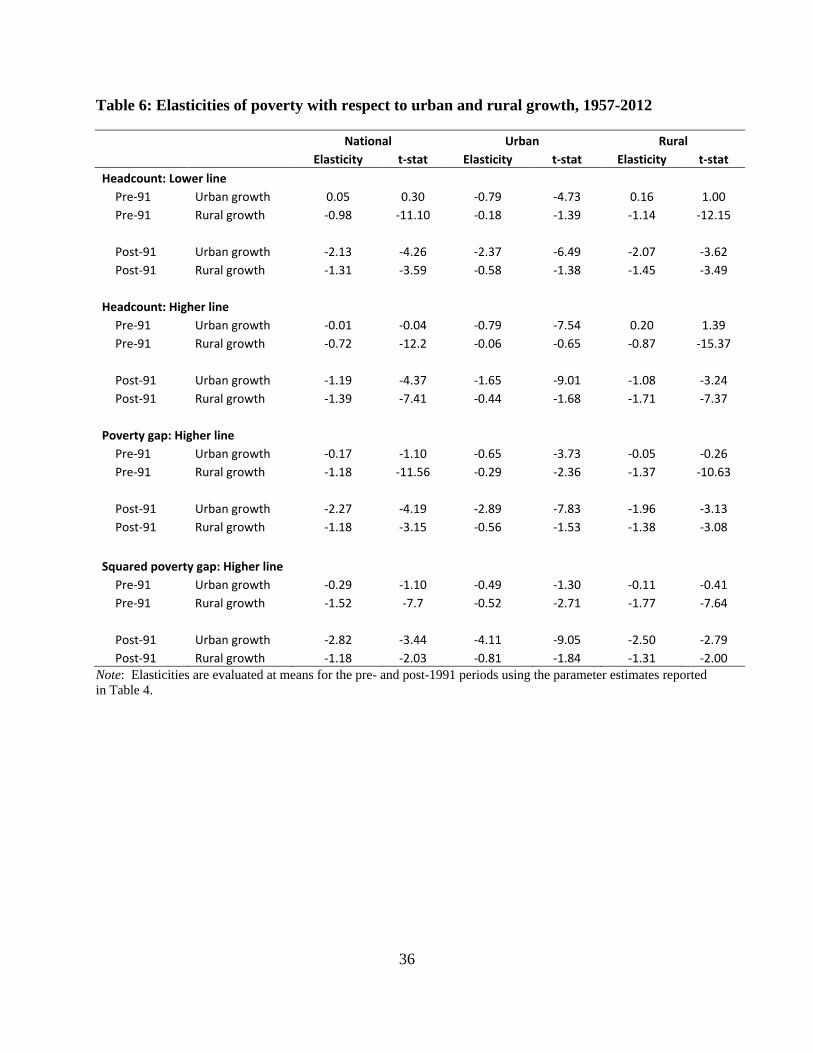
36

Table 6: Elasticities of poverty with respect to urban and rural growth, 1957-2012

National Urban Rural

Elasticity t-stat Elasticity t-stat Elasticity t-stat

Headcount: Lower line

Pre-91 Urban growth 0.05 0.30 -0.79 -4.73 0.16 1.00

Pre-91 Rural growth -0.98 -11.10 -0.18 -1.39 -1.14 -12.15

Post-91 Urban growth -2.13 -4.26 -2.37 -6.49 -2.07 -3.62

Post-91 Rural growth -1.31 -3.59 -0.58 -1.38 -1.45 -3.49

Headcount: Higher line

Pre-91 Urban growth -0.01 -0.04 -0.79 -7.54 0.20 1.39

Pre-91 Rural growth -0.72 -12.2 -0.06 -0.65 -0.87 -15.37

Post-91 Urban growth -1.19 -4.37 -1.65 -9.01 -1.08 -3.24

Post-91 Rural growth -1.39 -7.41 -0.44 -1.68 -1.71 -7.37

Poverty gap: Higher line

Pre-91 Urban growth -0.17 -1.10 -0.65 -3.73 -0.05 -0.26

Pre-91 Rural growth -1.18 -11.56 -0.29 -2.36 -1.37 -10.63

Post-91 Urban growth -2.27 -4.19 -2.89 -7.83 -1.96 -3.13

Post-91 Rural growth -1.18 -3.15 -0.56 -1.53 -1.38 -3.08

Squared poverty gap: Higher line

Pre-91 Urban growth -0.29 -1.10 -0.49 -1.30 -0.11 -0.41

Pre-91 Rural growth -1.52 -7.7 -0.52 -2.71 -1.77 -7.64

Post-91 Urban growth -2.82 -3.44 -4.11 -9.05 -2.50 -2.79

Post-91 Rural growth -1.18 -2.03 -0.81 -1.84 -1.31 -2.00

Note: Elasticities are evaluated at means for the pre- and post-1991 periods using the parameter estimates reported in Table 4.

37

Table 7: Decomposition of change in national poverty measures for the pre- and post-reform periods

Components of predicted change in poverty:

GR GU N K I

Total

change in

poverty

Total

predicted

change in

poverty

Rural

growth

Urban

growth

Population shift

with intra-sector

distributional

change

Population shift

holding intra-

sectoral

distribution

constant (Kuznets

effect)

Interaction

between

sectoral

poverty change

and population

shift

Headcount: lower line

Pre-91

Annual percentage change -1.38 -1.61 -0.72 -0.01 -0.84 -0.05 0.00

Share of pred. annual change 100.0 44.5 0.5 52.2 2.9 -0.1

Post-91

Annual %age change -6.47 -6.15 -2.88 -5.16 1.90 -0.02 0.01

Share of pred. annual change 100.0 46.9 83.9 -30.9 0.4 -0.2

Headcount: higher line

Pre-91

Annual percentage change -0.90 -1.16 -0.53 0.01 -0.60 -0.04 0.00

Share of pred. annual change 100.0 45.7 -1.0 52.0 3.2 0.1

Post-91

Annual percentage change -4.79 -4.67 -3.26 -2.93 1.55 -0.04 0.01

Share of pred. annual change 100.0 69.8 62.7 -33.1 0.9 -0.2

Poverty gap: higher line

Pre-91

Annual percentage change -1.90 -1.86 -0.86 -0.12 -0.89 0.00 0.00

Share of pred. annual change 100.0 46.3 6.3 47.7 -0.2 -0.2

Post-91

Annual percentage change -6.82 -6.49 -2.71 -5.32 1.52 0.01 0.01

Share of pred. annual change 100.0 41.7 82.0 -23.4 -0.2 -0.2

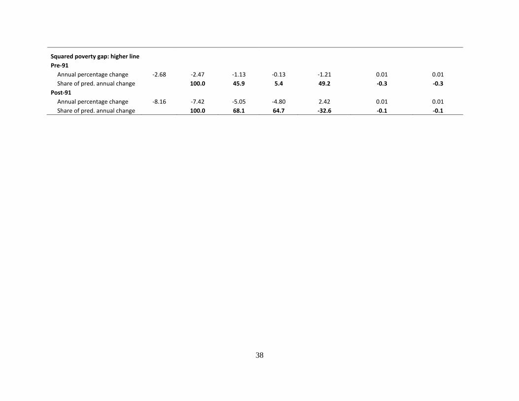
38

Squared poverty gap: higher line

Pre-91

Annual percentage change -2.68 -2.47 -1.13 -0.13 -1.21 0.01 0.01

Share of pred. annual change 100.0 45.9 5.4 49.2 -0.3 -0.3

Post-91

Annual percentage change -8.16 -7.42 -5.05 -4.80 2.42 0.01 0.01

Share of pred. annual change 100.0 68.1 64.7 -32.6 -0.1 -0.1

39

Table 8: Impacts of the sectoral composition of growth on the headcount index, 1957-2012

Change in log Headcount

(Lower Line)

Change in log Headcount

(Higher Line)

Unrestricted

model

Restricted

model

Unrestricted

model

Restricted

model

Variable or statistic Coeff. t-ratio Coeff. t-ratio Coeff. t-ratio Coeff. t-ratio

Pre-91 variables:

Primary sector growth -1.138 -4.59 -1.143 -4.58 -0.823 -3.41 -0.817 -3.43

Secondary sector growth 4.496 2.71 4.510 2.75 2.941 2.64 2.921 2.66

Tertiary sector growth -3.582 -3.20 -3.581 -3.28 -2.395 -3.30 -2.396 -3.42

Post-91 variables:

Primary sector growth -1.965 -0.22 -2.053 -0.33

Secondary sector growth -1.637 -0.32 -0.548 -0.15

Tertiary sector growth -1.510 -1.07 -1.360 -1.33

NDP growth -1.551 -2.79 -1.199 -2.95

Variables common to

both periods:

Change in log ratio of CPI

to NDP deflator 1.224 4.44 1.235 4.22 0.847 4.08 0.831 3.76

Change in binary var. for

an MRP estimate -0.320 -4.73 -0.321 -5.45 -0.219 -4.91 -0.224 -5.56

Number of observations 40 40 40 40

R2 0.656 0.655 0.660 0.658

Wald test of restrictions:

prob > F(2, 32)

Pre-91: π1 = π2 = π3 0.002 0.008

Post-91: π1 = π2 = π3 0.999 0.977

Note: The Table gives least squares estimates with heteroscedasticity and autocorrelation-consistent standard errors.

40

Table 9: Impacts of the sectoral composition of growth on poverty gap and squared

poverty gap indices, 1957-2012

Change in log Poverty Gap

(Higher Line)

Change in log Squared Poverty Gap

(Higher Line)

Unrestricted

model

Restricted

model

Unrestricted

model

Restricted

model

Variable or statistic Coeff. t-ratio Coeff. t-ratio Coeff. t-ratio Coeff. t-ratio

Pre-91 variables:

Primary sector growth -1.378 -5.47 -1.367 -5.56 -1.763 -5.13 -1.751 -5.30

Secondary sector growth 4.931 2.66 4.899 2.72 6.354 2.38 6.319 2.45

Tertiary sector growth -4.128 -3.50 -4.129 -3.64 -5.376 -3.30 -5.377 -3.43

Post-91 variables:

Primary sector growth -0.217 -0.02 1.747 0.15

Secondary sector growth -1.349 -0.25 -2.104 -0.30

Tertiary sector growth -1.856 -1.28 -2.138 -1.18

NDP growth -1.624 -2.86 -1.880 -2.71

Variables common to

both periods:

Change in log ratio of CPI

to NDP deflator 1.427 4.46 1.403 4.73 1.864 4.38 1.837 4.94

Change in binary var. for

an MRP estimate -0.354 -4.68 -0.351 -5.59 -0.458 -4.32 -0.448 -5.19

Number of observations 40 40 40 40

R2 0.668 0.666 0.652 0.648

Wald test of restrictions:

prob > F(2, 32)

Pre-91: π1 = π2 = π3 0.005 0.019

Post-91: π1 = π2 = π3 0.981 0.945

Note: The Table gives least squares estimates with heteroscedasticity and autocorrelation-consistent standard errors.

41

Table 10: Elasticities of poverty with respect to sectoral components of NDP, 1957-2012

Sector’s

share of

NDP

Headcount

(Lower line)

Headcount

(Higher line)

Poverty gap

(Higher line)

Squared poverty

gap (Higher Line)

Elasticity t-stat Elasticity t-stat Elasticity t-stat Elasticity t-stat

Pre-91:

Primary sector

growth 0.416 -0.48 -4.58 -0.34 -3.43 -0.57 -5.56 -0.73 -5.30

Secondary

sector growth 0.237 1.07 2.75 0.69 2.66 1.16 2.72 1.50 2.45

Tertiary sector

growth 0.347 -1.24 -3.28 -0.83 -3.42 -1.43 -3.64 -1.87 -3.43

Post-91:

Primary sector

growth 0.228 -0.35 -2.79 -0.27 -2.95 -0.37 -2.86 -0.43 -2.71

Secondary

sector growth 0.253 -0.39 -2.79 -0.30 -2.95 -0.41 -2.86 -0.48 -2.71

Tertiary sector

growth 0.519 -0.80 -2.79 -0.62 -2.95 -0.84 -2.86 -0.98 -2.71

Note: Elasticities are evaluated at means for the pre- and post-1991 periods using the parameter estimates of the restricted model reported in Tables 8 and 9.

42

Table 11: Decomposition of change in national poverty measures for the pre- and post-

reform periods (by NDP sector)

Components of predicted change in poverty:

Total

change in

poverty

Total

predicted

change in

poverty

Total

predicted

change in

poverty

without

population

growth

Primary

sector

NDP

growth

Secondary

sector

NDP

growth

Tertiary

sector

NDP

growth

NA

Deflator-

CPI drift

Headcount: lower line

Pre-91

Annual percentage change -1.38 -1.06 -2.45 -1.08 5.26 -6.69 0.07

Share of predicted annual

change 100.0 44.4 -215.1 273.6 -2.8

Post-91

Annual percentage change -6.47 -7.63 -10.24 -0.94 -2.42 -6.45 -0.37

Share of predicted annual

change 100.0 9.2 23.6 63.0 3.6

Headcount: higher line

Pre-91

Annual percentage change -0.90 -0.78 -1.80 -0.78 3.41 -4.47 0.05

Share of predicted annual

change 100.0 43.1 -189.6 249.0 -2.6

Post-91

Annual percentage change -4.79 -5.87 -7.89 -0.73 -1.87 -4.99 -0.25

Share of predicted annual

change 100.0 9.3 23.7 63.3 3.1

Poverty Gap: higher line

Pre-91

Annual percentage change -1.90 -1.42 -3.22 -1.30 5.71 -7.71 0.08

Share of predicted annual

change 100.0 40.3 -177.6 239.7 -2.4

Post-91

Annual percentage change -6.82 -8.02 -10.76 -0.99 -2.54 -6.76 -0.42

Share of predicted annual

change 100.0 9.2 23.6 62.8 3.9

Squared Poverty Gap:

higher line

Pre-91

Annual percentage change -2.68 -1.89 -4.23 -1.66 7.37 -10.04 0.10

Share of predicted annual

change 100.0 39.3 -174.1 237.2 -2.4

Post-91

Annual percentage change -8.16 -9.35 -12.52 -1.14 -2.94 -7.82 -0.54

Share of predicted annual

change 100.0 9.1 23.4 62.5 4.3

43

Figure 1: Net domestic product by sector and poverty rate

Source: Authors’ calculations. Figure 2: Trends in urban and rural inequality

Source and notes: Authors’ calculations. Locally-weighted smoothed scatter plots.

0

20

40

60

80

100

7.0

7.5

8.0

8.5

9.0

9.5

10.0

10.5

11.0

1950 1960 1970 1980 1990 2000 2010 2020

Net domestic product per capita(log, right axis)

Headcount index(%, left axis)

Urban population share(%, left axis)

Total

Primary

Second-ary

Tertiary

Lowerline

Upperline

25.0

27.5

30.0

32.5

35.0

37.5

40.0

42.5

45.0

1950 1960 1970 1980 1990 2000 2010 2020

Gin

i in

de

x (

%) Urban

Rural

44

Figure 3: Ratio of urban mean to rural mean consumption

Source: Authors’ calculations.

Figure 4: Poverty measures for India

Source: Authors’ calculations.

1.05

1.10

1.15

1.20

1.25

1.30

1.35

1.40

1.45

1950 1960 1970 1980 1990 2000 2010

Ra

tio

of u

rba

n m

ea

n to

ru

ral m

ea

n

(bo

th in

co

nsta

nt ru

ral p

rice

s)

0

10

20

30

40

50

60

70

1950 1960 1970 1980 1990 2000 2010 2020

RuralUrbanNational

He

ad

co

un

t in

de

x (

%, lo

we

r lin

e)

45

Figure 5: Convergence between rural and urban poverty measures

Note: Locally-weighted smoothed scatter plots.

Figure 6: Urbanization of poverty

Source: Authors’ calculations.

-4

0

4

8

12

16

20

1950 1960 1970 1980 1990 2000 2010 2020

Upper line Lower line

Ru

ral m

inu

s u

rba

n h

ea

dco

un

t in

de

x (

%)

Upper line

Lower line

0

4

8

12

16

20

24

28

32

36

1950 1960 1970 1980 1990 2000 2010 2020

Lower line

Upper line

Urb

an

sh

are

of th

e p

oo

r (%

)