1  

Poverty and Economic Decision-Making:

Evidence from Changes in Financial Resources at Payday*

LEANDRO S. CARVALHO, STEPHAN MEIER, AND STEPHANIE W. WANG

We study the effect of financial resources on decision-making. Low-

income U.S. households are randomly assigned to receive an online

survey before or after payday. The survey collects measures of

cognitive function and administers risk and intertemporal choice

tasks. The study design generates variation in cash, checking and

savings balances, and expenditures. Before-payday participants

behave as if they are more present-biased when making

intertemporal choices about monetary rewards but not when making

intertemporal choices about non-monetary real-effort tasks. Nor do

we find before-after differences in risk-taking, the quality of

intertemporal decision-making, the performance in cognitive

function tasks, or in heuristic judgments.

*Meier: Columbia University, Graduate School of Business, Uris Hall, 3022 Broadway, New York, NY 10027 (email:

sm3087@columbia.edu). This paper benefited from comments from Dan Benjamin, Jeffrey V. Butler, Andrew Caplin,

Dana Goldman, Ori Heffetz, Sendhil Mullainathan, Eldar Shafir, Jesse Shapiro, Charlie Sprenger, and participants in

seminars and conferences where it was presented. Carvalho thanks the RAND Roybal Center for Finacial Decisionmaking

and the Resource Center for Minority Aging Research (RCMAR) at the University of Southern California’s Schaeffer

Center, Meier thanks the Columbia Business School, and Wang thanks the University of Pittsburgh Central Research

Development Fund for generous research support.

  2  

The poor often behave differently from the non-poor. For example, they are

more likely to make use of expensive payday loans and check-cashing services, to

play lotteries, and to repeatedly borrow at high interest rates.1 The debate about

the reasons underlying such differences has a long and contentious history in the

social sciences; the two opposing views are that either the poor rationally adapt

and make optimal decisions for their economic environment or that a “culture of

poverty” shapes their preferences and makes them more prone to mistakes.2

Among economists, this debate has been manifest in lingering questions of

whether the poor are more impatient, more risk averse, and have lower self-

control, which could trap them into a cycle of poverty.3 A third view emerges

from the work of Mullainathan, Shafir, and co-authors.4 They argue that scarcity,

defined as “having less than you feel you need” (Mullainathan and Shafir 2013

pg. 4), impedes cognitive functioning, which in turn may lead to decision-making

errors and myopic behavior.5

Empirically, there are major challenges in isolating the causal effects of

economic circumstances on decision-making. There may not be only a reverse

causality bias – that is, the economic decisions one makes determine one’s

economic circumstances – but also be unobserved individual characteristics, such

as innate cognitive ability, confounding the relationship between economic

circumstances and decision-making. Identification of the effects of poverty on

time preferences is further complicated by the possibility that poverty may affect

credit constraints and arbitrage opportunities, which in turn could influence

intertemporal choices (e.g., Frederick et al. 2002).

                                                                                                                         1 Rhine et al. 2006; Ananth et al. 2007; Haisley et al. 2008; Bertrand and Morse 2011; Dobbie and Skiba 2013. 2 E.g., Schultz 1964 and Lewis 1965. See Bertrand et al. 2004 and Duflo 2006 for more recent perspectives. 3 Lawrance 1991; Banerjee and Mullainathan 2010; Tanaka et al. 2010; Spears 2011; Gloede et al. 2012; Bernheim et al. 2013; Carvalho 2013; Haushofer et al. 2013. 4 Shah et al. 2012; Mullainathan and Shafir 2013; Mani et al. 2013. 5 A number of studies document an association between cognitive ability and economic choices (e.g., Burks et al. 2009; Dohmen et al. 2010, Benjamin et al. 2013).

  3  

This paper uses changes in financial resources at payday to empirically

investigate whether financial resources have a causal effect on economic

decision-making. Previous work has documented that the expenditures and the

caloric intake of some households increase sharply at payday (e.g., Stephens

2003, 2006; Huffman and Barenstein 2004; Shapiro 2005).

To exploit the sharp change in financial resources at payday, we designed and

administered online surveys: 1,191 participants with annual household income

below $40,000 were randomly assigned to a group surveyed shortly before

payday (hereafter, the before-payday group) or shortly after payday (hereafter, the

after-payday group). We then collected measures of cognitive function and

administered incentivized risk choice and incentivized (monetary and non-

monetary) intertemporal choice tasks. Our goal was to investigate whether the

before-payday group would behave differently from the after-payday group.

Like the previous related experimental studies (e.g., Spears 2011; Mani et al.

2013), the variation in financial resources that we use to identify our effects is

temporary, anticipated, and perhaps equally important, is anticipated to be

temporary. The participants surveyed before payday knew when their next

payment would arrive and when more money would come in. Thus, our study

speaks to the effects of sharp but short-lived variations in financial resources. It is

this particular impoverishment before payday that we allude to when we refer to

“poverty”. It is still an open question how our findings generalize to similar

effects for a permanent shift in permanent income.

Our results contribute to at least two important strands of literature: First, the

results provide insights on the effects of poverty on time and risk preferences,

suggesting that there are no such relationships. Although we find that the before-

payday group behaved as if they were more present-biased when making

intertemporal choices about monetary rewards, this behavior is most likely

explained by differences in liquidity constraints, since the two groups made

  4  

similar intertemporal choices about non-monetary rewards. They also made

similar risk choices, suggesting that economic circumstances do not affect the

willingness to take risks.

Second, our findings contribute to the debate on poverty and decision-making

(e.g., Spears 2011; Mullainathan and Shafir 2013), but do not support the

hypothesis that financial strain per se impedes cognitive function and worsens the

quality of decision-making. We find that participants surveyed before and after

payday performed similarly on a number of cognitive function tasks. Furthermore,

we find no difference in the likelihood of heuristic judgment and no significant

differences across the two groups in the quality of the decision-making, as

measured in terms of the consistency of the intertemporal choices.

The paper is structured as follows. Section I discusses the study design;

Section II presents the results, followed by a concluding discussion.

I. Study Design

We collected data using the RAND-USC American Life Panel (ALP), an

ongoing internet panel with respondents aged 18 and over living in the United

States. About twice a month, respondents receive an email with a request to visit

the ALP site and complete questionnaires. Respondents without Internet access at

the time of recruitment are provided laptops and an internet access subscription,

partly mitigating any concerns about selection bias due to internet access. The

panel recently has been expanded to include more than 2,000 members of

vulnerable populations drawn from zip codes with a large fraction of low-income,

low-education, or minority populations.

We restricted our study sample to panel members with an annual household

income of $40,000 or less. More than one third of the sample had an annual

  5  

family income below $15,000 and 45 percent had less than $20,000.6 Other

results indicate that the study sample had low socioeconomic status (hereafter,

SES): more than 45% had zero or negative non-housing wealth and 60% had zero

or negative housing wealth.7 Other characteristics associated with poverty were:

18% of our sample were unemployed, one-fifth reported being disabled, and only

37% were working at the time of the survey. Approximately 17% did not have a

checking or savings account (compared to a 7% national average, FINRA 2013),

and more than 45% did not have a credit card (compared to a 29% national

average, FINRA 2013). Finally, because of a shortage of money, more than half

of them had experienced (at least) one of the following in the 12 months before

the study: could not pay electricity, gas, or phone bills; could not pay for car

registration or insurance; pawned or sold something; went without meals; were

unable to heat home; sought assistance from welfare or community organizations;

sought assistance from friends or family; or took a payday loan. (See Appendix C

for more details about the socioeconomic status of the sample.)

The study consisted of one baseline and one follow-up survey. The baseline

survey collected information that was used to determine participants’ paydays.

The opening dates of the follow-up survey, which were specific to each study

participant, depended on the participant’s payday and her random assignment.8

Specifically, the follow-up survey opened seven days before payday for

participants assigned to the before-payday group and one day after payday for

participants assigned to the after-payday group.9 Participants were sent emails

informing them when the survey was available. The follow-up survey measured

various aspects of decision-making for the two randomly assigned groups.

                                                                                                                         6 These figures were calculated using the sample of 1,098 participants who started the follow-up survey. 7 See footnote of table C2 in Appendix C for more details about the wealth measures. 8 Spears (2012) used a similar design in which recipients of South Africa’s old age pension were randomly assigned to be surveyed before or after receiving the monthly pension payment to study cognitive limits and intertemporal choices. 9 For a participant whose payday fell on January 15, the survey would be available at January 8 at 12:00:01am if she were assigned to the before-payday group and at January 16 at 12:00:01am if she were assigned to the after-payday group.

  6  

A. The Baseline Survey and Study Sample

The baseline survey collected data on the dates and amounts of all payments

that the participant (and his/her spouse) expected to receive during January

2013.10 (See Appendix A for screenshots of the baseline survey.) The study then

focused on subjects who provided complete information about the number and

dates of payments, and on those who anticipated receiving fewer than five

payments from a single income source in January 2013.11 (See Appendix D for

more details about the payments.)

These data were then used to identify the payday of each participant payday.

If the largest payment came two weeks or more after the previous payment, the

payday was set as the date of this largest payment. Otherwise, the payday was set

as the date that followed an interval of 14 days or more without any other

payments. Two hundred and eight participants whose payments were all less than

2 weeks apart were dropped from the study sample. (See Appendix E, which

gives details about sample restrictions and survey nonresponse, for the flow of

participants through the study.)

B. Randomization and Treatment Compliance

The remaining 1,191 study participants then were randomly assigned to the

before-payday group or the after-payday group using a stratified sampling and re-

randomization procedure (see Appendix F for more details). We stratified on

whether at baseline participants strongly agreed with the statement “I live from

paycheck to paycheck” and on whether they anticipated receiving only one

payment in January 2013, because we planned to check whether the effects would

                                                                                                                         10 To test the survey design, we conducted a pilot in May of 2010 with about 200 respondents; we randomly assigned whether a participant was surveyed before or after payday. 11 The rationale for dropping respondents who anticipated five payments or more from a single income source is that their income should be spread out sufficiently over time, making it easier for them to smooth consumption.

  7  

be any different for those participants whose economic circumstances could be

expected to change more sharply at payday.12 The randomization was successful

in making assignment to the before-payday group orthogonal to observable

baseline characteristics (see Appendix F).

The study design generated variation in the time at which participants started

and finished the survey. The median respondent assigned to the before-payday

group started the survey 2.4 days before payday and completed it 1.5 days before

payday.13 The median respondent assigned to the after-payday group started the

survey 4.4 days after payday and completed it 5 days after payday. The

differences across the two groups were all statistically significant at 1%.

Note that although the study design allowed us to manipulate when the survey

was made available to a participant, we did not have control over when the

participant started (or finished) the survey. Consequently, it was expected that

there would be imperfect compliance, in the sense that some of the participants

assigned to the before-payday group could effectively start (or finish) the follow-

up survey after payday. In practice, about 70% of the participants assigned to the

before-payday group started the survey before payday, while 63% completed the

survey before payday.14 By construction, all participants assigned to the after-

payday group started the survey at least one day after payday (see the first table in

Appendix J for more detailed results). In our analysis, we estimate intent-to-treat

effects, exploiting the random assignment to the before-payday group as a source

of exogenous variation in starting the survey before payday.15

                                                                                                                         12 We also stratified on whether the respondent had some college education and on whether the survey would open before 12/31/2012 if the respondent were assigned to the before-payday group. 13 Because participants were not required to complete the survey in just one sitting, the time interval between when they started the survey and when they completed it may have been much longer than the time it would effectively take to complete the survey without interruption. The median participant took 51 minutes to complete the survey. 14 Results are similar if the sample is restricted to participants who started the survey within 7 days of its opening. See Appendix I. 15 To take into account the imperfect compliance, one could scale up the estimates by instrumenting for starting the survey before payday using the assignment into the before-payday. But it is an open question as to how many days after payday participants re-enter a period of low financial resources. For this reason we opt for presenting intent-to-treat estimates.

  8  

C. The Follow-up Survey

The follow-up survey collected measures of (1) economic decision-making,

(2) cognitive function, and (3) financial circumstances. We discuss them here

briefly; for more details and screenshots of the follow-up survey, see Appendix B.

(1) Economic Decision-Making. Two intertemporal choice tasks – one with

monetary rewards and one with non-monetary rewards – and a risk choice task

were administered. In the monetary intertemporal choice task, a variant of

Andreoni and Sprenger (2012)’s Convex Time Budget (CTB), participants were

asked to allocate an experimental budget of $500 between two payments with pre-

specified dates. The amount of the second payment included interest. Participants

had to make 12 of these choices in which the experimental interest rate varied

(0%, 0.5%, 1%, or 3%), as did the mailing date of the first payment (either today

or in four weeks) and the time delay between the two payments (four weeks or

eight weeks). Approximately one percent of participants were randomly selected

to be paid based on one of their 12 choices.

Another task required participants to make intertemporal choices regarding

real effort (similar to Augenblick et al. 2013) in order to address concerns about

the use of monetary rewards in measuring time discounting (e.g., Frederick et al.

2002). Specifically, participants had to choose between completing a shorter

survey within 5 days or a longer (30-minute) survey within 35 days. They were

asked to make five such choices, with the length of the sooner survey gradually

increasing (from 15 to 18, 21, 24, and 27 minutes). Five similar choices followed,

in which the deadlines were shifted from 5 to 90 days (shorter) and 35 to 120 days

(longer). Approximately one percent of the participants were randomly selected to

  9  

have one of their 10 choices implemented (i.e., “implementation surveys” were

sent to those selected participants).16

To analyze the willingness to take risks, we presented a risk choice task

designed by Eckel and Grossman (2002). Here, participants were asked to choose

one of six lotteries, each with a 50-50 chance of paying a lower or a higher

reward. The six (higher/lower) pairings were ($28/$28), ($36/$24), ($44/$20),

($52/$16), ($60/$12), and ($72/$0). Approximately 10 percent of participants

were randomly selected to actually be paid according to their choices.

Two additional tasks measured loss aversion, as in Fehr and Goette (2007),

and simplicity seeking, as in Iyengar and Kamenica (2010). The latter task was

incentivized; the former was not.

(2) Cognitive Function. To measure cognitive function, we used the Flanker

task, a working memory task, and the Cognitive Reflection Test (CRT). In the

Flanker task, a well-established inhibitory control task that is part of the NIH

toolbox (Zelazo et al. 2013), subjects are supposed to focus on a central stimulus

while trying to ignore distracting stimuli (Ericksen and Ericksen 1974). In the

working memory task, participants are asked to recall a sequence of colors; the

length of the sequence gradually increases if the participant can successfully

repeat a given sequence. The CRT measures one’s ability to suppress an intuitive

and spontaneous incorrect answer and to instead give the deliberative and

reflective correct answer (Frederick 2005). In addition to these tests of cognitive

function, we have other measures of participants’ cognitive abilities, including

both fluid and crystallized intelligence, which were collected in previous ALP

surveys. The final table in Appendix I shows that our measures of cognitive

function are strongly correlated with these other measures of cognitive ability.

                                                                                                                         16 If they completed the survey before the deadline, they received a $50 Amazon gift card and $20 was added to the quarterly check they regularly received for answering surveys. The dates of these payments were fixed and thus did not depend on when respondents finished the implementation surveys (as long as they were completed before the deadline).

  10  

We also included two items to measure the use of heuristics. One question

from Toplak et al. (2011) captures whether the respondent believes in the

gambler’s fallacy: that is, the incorrect expectation that after one particular

realization of a random variable the next realization of this same random variable

will be different. Sensitivity to framing was measured using the “disease

problem” proposed by Tversky and Kahneman (1981).

(3) Financial circumstances. The follow-up survey included questions on cash

holdings, checking and savings accounts balances, and expenditures, which

permit checking if the study design generated variation in financial circumstances.

II. Results

Section IIA below shows that the study design generated substantial

differences in the financial resources of the before-payday and after-payday

groups. We then examine whether these differences in financial resources were

accompanied by differences in intertemporal choices (Section IIB), risk choices

(Section IIC), consistency of intertemporal choices (Section IID), and cognitive

functions (Section IIE).

A. Cash Holdings, Checking and Savings Balances, and Expenditures

Table 1 indicates that the before-payday group had fewer financial resources

than the after-payday group: on average, the before-payday group had $114 less

in cash (52% of the after-payday group mean) and $1,947 less in their checking

and savings accounts (29% of the after-payday group mean). The before-payday

group also reported having spent $553 less in the previous seven days (48% of the

after-payday group mean), which is consistent with well-documented results that

expenditures increase sharply at payday (e.g., Stephens 2003, 2006).

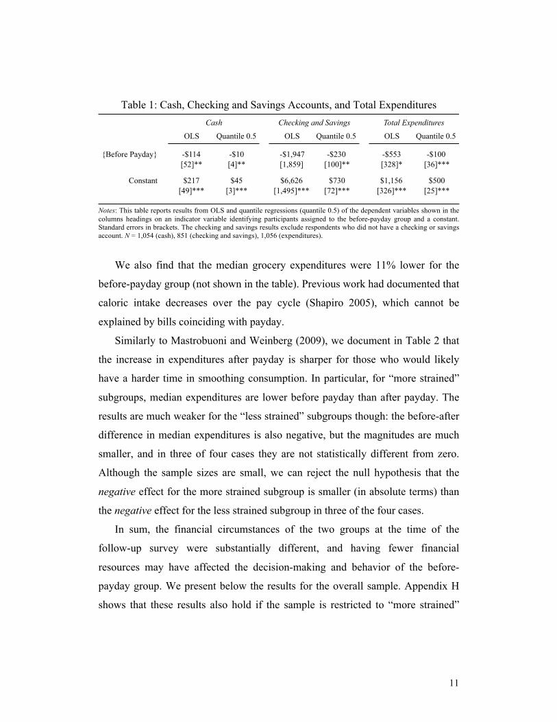
  11  

Table 1: Cash, Checking and Savings Accounts, and Total Expenditures

Notes: This table reports results from OLS and quantile regressions (quantile 0.5) of the dependent variables shown in the columns headings on an indicator variable identifying participants assigned to the before-payday group and a constant. Standard errors in brackets. The checking and savings results exclude respondents who did not have a checking or savings account. N = 1,054 (cash), 851 (checking and savings), 1,056 (expenditures).

We also find that the median grocery expenditures were 11% lower for the

before-payday group (not shown in the table). Previous work had documented that

caloric intake decreases over the pay cycle (Shapiro 2005), which cannot be

explained by bills coinciding with payday.

Similarly to Mastrobuoni and Weinberg (2009), we document in Table 2 that

the increase in expenditures after payday is sharper for those who would likely

have a harder time in smoothing consumption. In particular, for “more strained”

subgroups, median expenditures are lower before payday than after payday. The

results are much weaker for the “less strained” subgroups though: the before-after

difference in median expenditures is also negative, but the magnitudes are much

smaller, and in three of four cases they are not statistically different from zero.

Although the sample sizes are small, we can reject the null hypothesis that the

negative effect for the more strained subgroup is smaller (in absolute terms) than

the negative effect for the less strained subgroup in three of the four cases.

In sum, the financial circumstances of the two groups at the time of the

follow-up survey were substantially different, and having fewer financial

resources may have affected the decision-making and behavior of the before-

payday group. We present below the results for the overall sample. Appendix H

shows that these results also hold if the sample is restricted to “more strained”

{Before Payday}

Constant

OLS Quantile 0.5 OLS Quantile 0.5 OLS Quantile 0.5

-$114 -$10 -$1,947 -$230 -$553 -$100[52]** [4]** [1,859] [100]** [328]* [36]***

$217 $45 $6,626 $730 $1,156 $500[49]*** [3]*** [1,495]*** [72]*** [326]*** [25]***

Cash Checking and Savings Total Expenditures

  12  

subgroups of participants whose financial circumstances one would expect to

change more sharply at payday or to those who made less than $20,000 per year.

Table 2: Expenditures for More Financially Strained and Less Strained Subgroups

Notes: This table reports estimated coefficients from quantile regressions (quantile 0.5) of total expenditures on an indicator for the before-payday group and a constant. Separate results for subgroups more and less financially strained are shown respectively in columns (1) and (2). The four measures of financial strain are: A) receiving one payment over the month (versus multiple payments); B) having gone through a financial hardship in the previous 12 months: could not pay electricity, gas, or phone bills, car registration or insurance; pawned or sold something; went without meals; were unable to heat home; sought assistance from welfare or community organizations, friends or family; or took a payday loan; C) being in the lower half of the wealth distribution; and 4) having strongly agreed with the statement “I live from paycheck to paycheck.”The last column reports the p-value of a one-sided hypothesis test that the negative effect for the more strained subgroup is smaller (in absolute terms) than the negative effect for the less strained subgroup. Standard errors are not reported in the table (available upon request). Number of observations in parentheses.

B. Intertemporal Choices

Economists have long debated whether the poor have higher discount rates

(e.g., Lawrance 1991, Carvalho 2013; Haushofer et al. 2013). Because the poor

Quantile Regression (Quantile 0.5)

P-value TestTotal Expenditures Last 7 Days(1) (2) (1) ≥ (2)

{Before Payday}Constant

{Before Payday}Constant

{Before Payday}

One Payment (423) Multiple Payments (633)

-$200*** -$60 0.03**$500*** $460***

Financial Hardship (547) No Hardship (508)

-$200*** -$50 0.01**$600*** $400***

Bottom Half (509) Upper Half (518)

-$109** -$92* 0.42

Wealth Distribution

Constant

{Before Payday}Constant

$500*** $460***

Strongly Agree (557) Others (499)

-$150*** -$50 0.07*$550*** $400***

"I Live from Paycheck to Paycheck"

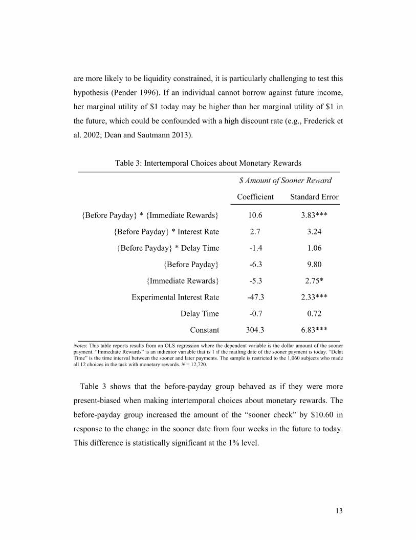
  13  

are more likely to be liquidity constrained, it is particularly challenging to test this

hypothesis (Pender 1996). If an individual cannot borrow against future income,

her marginal utility of $1 today may be higher than her marginal utility of $1 in

the future, which could be confounded with a high discount rate (e.g., Frederick et

al. 2002; Dean and Sautmann 2013).

Table 3: Intertemporal Choices about Monetary Rewards

  Notes: This table reports results from an OLS regression where the dependent variable is the dollar amount of the sooner payment. “Immediate Rewards” is an indicator variable that is 1 if the mailing date of the sooner payment is today. “Delat Time” is the time interval between the sooner and later payments. The sample is restricted to the 1,060 subjects who made all 12 choices in the task with monetary rewards. N = 12,720.

Table 3 shows that the before-payday group behaved as if they were more

present-biased when making intertemporal choices about monetary rewards. The

before-payday group increased the amount of the “sooner check” by $10.60 in

response to the change in the sooner date from four weeks in the future to today.

This difference is statistically significant at the 1% level.

Coefficient Standard Error

{Before Payday} * {Immediate Rewards} 10.6 3.83***

{Before Payday} * Interest Rate 2.7 3.24

{Before Payday} * Delay Time -1.4 1.06

{Before Payday} -6.3 9.80

{Immediate Rewards} -5.3 2.75*

Experimental Interest Rate -47.3 2.33***

Delay Time -0.7 0.72

Constant 304.3 6.83***

$ Amount of Sooner Reward

  14  

There are no other statistically significant differences across the two groups

and we can rule out economically meaningful differences. In Appendix K we use

the CTB framework to estimate utility-function parameters that better quantify the

differences in behavior across the two groups. We can rule out that the before-

after (absolute) difference in the utility curvature parameter was greater than

0.003.17 The discount rates are estimated with less precision, but we still can rule

out that the before-payday group had an annual discount rate 1.05 percentage

points higher than the after-payday group.18

Although the result that the before-payday group behaved as if it was more

present-biased is consistent with the interpretation that scarcity reduces self-

control, it is also possible that such behavior could be explained by before-after

differences in liquidity constraints. Augenblick et al. (2013) argue that

intertemporal choices about real effort are better suited than intertemporal choices

about monetary rewards to capture dynamic time inconsistent preferences,

because the latter are subject to several confounds. In Table 4 we analyze

subjects’ intertemporal choices between a shorter survey sooner and a longer

survey later. We estimate an interval regression where the dependent variable is a

measure of individual discount rate (as in Meier and Sprenger 2010).19

We find that the two groups behaved similarly in making intertemporal

choices about a costly real-effort task, namely choosing between answering a

shorter survey sooner and a longer survey later. Both groups displayed behavior

that was consistent with present-bias: the implied monthly discount rate was 9

percentage points higher when the shorter-sooner survey had to be completed

within five days (as opposed to 90 days).

                                                                                                                         17 The CTB framework assumes constant relative risk aversion (CRRA) risk preferences, where 𝑢(𝑐) = 𝑐!/  𝛼 and 𝛼 is the utility curvature parameter. This figure is however sensitive to the particular assumptions about background consumption. 18 The after-payday group is estimated to have an annual discount rate of 9.4%. 19 Let X be the duration of the longest sooner survey the subject chose over the later survey. The (lower bound, upper bound) of the discount rate intervals were: (15/30,18/30) for X = 15; (18/30,21/30) for X = 18; (21/30,24/30) for X = 21; (24/30,27/30) for X = 24, and (27/30,1) for X = 27. The interval was (0,15/30) for those who always chose the later survey.

  15  

Table 4: Intertemporal Choices about Real Effort

  Notes: This table reports estimates from an interval regression where the dependent variable is the interval measure of the individual discount rate (IDR). Two IDRs are estimated for each subject; one for each time frame. “Immediate Task” is an indicator variable for the “5 days (sooner) x 35 days (later)” time frame. Standard errors clustered at the individual level. The sample is restricted to the 1,025 subjects who made all 10 choices in the non-monetary intertemporal task. N = 2,050.

However, there is no evidence of differential present-bias in this task.

Although one should be cautious in comparing intertemporal choices about

monetary rewards to intertemporal choices about real effort, this result suggests

that liquidity constraints may explain why the before-payday group behaved as if

it was more present-biased in the monetary intertemporal choice task. Even

though one could worry that the before-payday and after-payday groups may have

had different time constraints, we find no evidence to support such hypothesis.20

C. Risk Choices

As Table 5 shows, the before-payday and after-payday groups make similar

risk choices.21 The before-payday group behaves as if they are less risk averse,

but the differences are small and not statistically significant.22 The before-payday

                                                                                                                         20 For example, there is no statistically significant difference in how much time the two groups took to complete the follow-up survey or in how likely they were to start or complete the follow-up survey. The result of no different present-bias also holds if the sample is restricted to participants who not were working at the time of the follow-up survey. 21 The CRRA parameter intervals are: (-∞,0) for those who chose (70/2); (0,0.50) for (60/12); (0.50,0.71) for (52/16); (0.71,1.16) for (44/20); (1.16,3.46) for (36/24); and (3.46,+∞) for (28,28). 22 The p-value of a Wilcoxon rank-sum test that the risk choices of two groups were from the same distribution was 0.42.

Monthly Discount Rate

{Before Payday} * {Immediate Task} -0.03[0.025]

{Before Payday} 0.02[0.027]

{Immediate Task} 0.09(5-day deadline for short-sooner survey) [0.018]***

Constant 0.31[0.019]***

  16  

and after-payday groups also make similar choices in two additional risk-related

choice tasks: there were no before-after differences in either the loss aversion or

the simplicity seeking experimental tasks (see Appendix G).

Table 5: Risk Choices and Consistency in Intertemporal Choices

  Notes: The first column reports estimates from an interval regression where the dependent variable is the interval measure of the coefficient of relative risk aversion. The last two columns report results from OLS regressions where the dependent variable is a measure of consistency in intertemporal choices. In the second column, which investigates consistency in intertemporal choices about monetary rewards, the dependent variable is the fraction of times in which the subject increased (or kept constant) the later reward in response to an increase in the experimental interest rate (Gine et al. 2013). In the last column, which investigates consistency in intertemporal choices about real effort, the dependent variable is 1 if the participant had at most one switching point for each time frame (Burks et al. 2009). Robust standard errors in brackets.

The change in financial resources at payday could affect the willingness to

take risks in two ways. First, liquidity constraints could increase the marginal

utility of consumption and reduce the willingness to take risks. On the other hand,

scarcity could have a direct effect on risk preferences per se (e.g., Tanaka et al.

2010; Gloede et al. 2012). These effects could partly offset each other if scarcity

reduced risk aversion.23

                                                                                                                         23 Moreover, liquidity constraints should not influence individuals’ risk choices if subjects were “narrowly bracketing” when making their risk choices (see, e.g., Tversky and Kahneman 1981, Rabin and Weizsacker 2009).

Risk Choice Task

% of Times Responded (Non-Monetary)CRRA to Increase in Interest by 1 if at Most One

Parameter Increasing $ Later Reward Switching Point

{Before Payday} -0.10 -0.02 -0.01[0.152] [0.013] [0.023]

Constant 1.66 0.84 0.84[0.110]*** [0.009]*** [0.016]***

Consistency in Intertemporal Choices

N 1,064 1,060 1,025

  17  

D. Consistency of Intertemporal Choices

To investigate whether economic circumstances affect the quality of decision-

making, we first look at consistency in the intertemporal choices and then

examine performance in the cognitive function tasks.

In the task with monetary rewards (i.e., CTB), the assumptions of additive

separability and monotonicity allow for a strong prediction: the amount allocated

to the later payment should increase with the experimental interest rate. Following

Gine et al. (2013), we measure consistency as the fraction of times in which

subjects increased (or kept constant) the later reward in response to an increase in

the experimental interest rate.24 In the task with non-monetary rewards, we follow

Burks et al. (2009). We define subjects as being consistent if they had at most one

switching point (for each time frame). Our outcomes of interest are the measures

of consistency in each task.

As the last two columns of Table 5 show there are no statistically significant

differences in the consistency of intertemporal choices. In the task with monetary

rewards, the before-payday group was two percentage points less likely to be

consistent than the after-payday group (who had an 84% consistency rate), but

this difference was not statistically significant. The before-after difference in the

non-monetary intertemporal task also was not statistically significant.25

In terms of heuristics, there are no differences in sensitivity of the two groups

to framing, or how likely they were to succumb to the gambler’s fallacy. These

results are shown in Appendix G.

                                                                                                                         24 Following Gine et al. (2013), we divided the twelve decisions of each subject into 9 pairs, where each element of the pair was the amount allocated to the more delayed payment. The first element was the amount allocated under interest rate 𝑟! and the second element was the amount allocated under interest rate 𝑟!, where 𝑟! was the next highest interest after 𝑟! (so for example 𝑟! = 0%and 𝑟! =0.5%). For each subject there were 9 pairs, 3 for each time frame. The pair was identified as consistent if the later reward under 𝑟! was greater or equal to the later reward under 𝑟!. 25 Nor do we find a difference in the consistency in the loss aversion task. The mean for the after-payday group was 0.811 and the before-after difference was -0.004 with a p-value of 0.86.

  18  

E. Cognitive Function

As shown in Table 6, the before-payday and after-payday groups performed

similarly in the tasks and tests used to measure cognitive function. On the Flanker

task, participants assigned to the before-payday group were on average 2 percent

slower in their response time than the after-payday group, but they were also 1

percentage point more likely to respond correctly. None of these differences were

statistically significant at the 10% level. The before-payday group performed

slightly better in the working memory task and in the Cognitive Reflection Test

(Frederick 2005), but, again, these differences were not statistically significant.26

Table 6: Cognitive Function  

Notes: See pages 8 and 9 for a description of the Flanker and working memory tasks, and the cognitive reflection test. This table reports results from OLS regressions of the dependent variables shown in the column headings on an indicator variable for the before-payday group and a constant (the regressions in the first two columns also include trial-specific dummies). Response time in the Flanker task was measured in milliseconds. Memory span is the length of the longest list of colors the participant was able to reproduce. In the first two columns the standard errors are clustered at the individual level. In the last two robust standard errors are estimated.

These results contrast with the findings of Mani et al. (2013) who compared

the performance of sugar cane farmers in India in related cognitive function tasks

during the pre-harvest season, when they supposedly have fewer resources, and

during the post-harvest season. They found for example that farmers spent 10.8%

                                                                                                                         26 Appendix H shows that these results hold if the sample is restricted to participants who made less than $20,000 per year. Mani et al. (2013) found effects of scarcity on cognitive function for a U.S. population making more than $20,000 per year.

Working Memory Cog. Reflection

Ln(Time) % Correct Memory Span % Correct

{Before Payday} 0.02 0.01 0.02 0.01[0.028] [0.010] [0.239] [0.014]

Constant 7.16 0.92 4.69 0.11[0.029]*** [0.010]*** [0.164]*** [0.010]***

N 20,557 20,557 1,038 1,045

Inhibitory Control (Flanker)

  19  

more time on the Stroop task before the harvest than after the harvest, and that

farmers were 1.03 percentage points less likely to respond correctly before the

harvest than after the harvest. A useful exercise is to compare our observed

before-after differences in performance on the Flanker task to the pre-post harvest

differences in performance on the Stroop task that Mani et al. (2013) observed.

Our confidence intervals imply that in the Flanker task, in the worst case

scenario, the before-payday group was 7.2% slower and 1.23 percentage points

less likely to respond correctly than the after-payday group. Thus, we can rule the

effect that Mani et al. (2013) observed on the Stroop time. However, the lower

bound of our 95% confidence interval is comparable to their point estimates of the

harvest effect on the fraction of correct responses.27

The difference between our results and Mani et al. (2013) suggest that we

need to refine our understanding of how limited resources affect cognitive

functioning. We showed that short-term variation in financial resources does not

deterministically lead to cognitive deficits and decision-making mistakes in

contrast with what previous studies found. As suggested by Mullainathan and

Shafir (2013), scarcity per se may not be enough: “[t]he feeling of scarcity is

distinct from its physical reality. Physical limits, of course, play a role…[b]ut so

does our subjective perception….” (pg. 11). While it is challenging to

conceptualize and measure this subjective perception of scarcity, preliminary

results from our own study suggest that the mapping from scarce resources to the

subjective perception of scarcity is not trivial (see Table J2 in Appendix J). While

it is beyond the scope of this paper, future research should a) focus on how to

measure subjective perception of scarcity reliably and b) investigate whether such

perception must be present for financial scarcity to affect cognitive functioning.

                                                                                                                         27 One important caveat: because Mani et al. (2013) do not provide estimates of the difference in income between the pre-harvest and post-harvest seasons, it is not possible to properly scale their effects to account for pre-post harvest differences in income which they rely on that may be greater (or smaller) than the before-after payday differences in income we rely on. Similarly, these calculations are based on intent-to-treat estimates that do not correct for imperfect compliance.

  20  

III. Discussion and Conclusion

In this paper, we use the sharp change in financial resources at payday for a

low-SES population to examine the causal effects of financial resources on

decision-making. Thus, ours is the first study we know of that provides

experimental evidence on whether financial resources affect the economic

decision-making of poor U.S. families.

Our results indicate that scarce resources indeed can affect one’s willingness

to delay gratification: before-payday participants behaved as if they were more

present-biased when making choices about monetary rewards. However, any

present-biased behavior was the same before and after payday when the

participants had to choose a costly real-effort task. Taken together, these results

suggest that the observed difference in the monetary intertemporal choice most

likely is due to liquidity constraints, not to poverty reducing one’s self-control.

Nor do our results support the hypothesis that financial strain by itself worsens

the quality of decision-making. Even though there are substantial differences in

financial resources before and after payday, we find no evidence that the

willingness to take risks, the quality of decision-making (measured in terms of the

consistency of the intertemporal choices), or being prone to heuristic judgments

(gambler’s fallacy and framing) differs across the before-payday and after-payday

groups. Furthermore, we do not find before-after differences in key aspects of

cognitive functions, such as inhibitory control or working memory.

In conjunction with the previous literature, our findings suggest that more

needs to be done to understand the effects on cognitive functions and economic

decision-making of the interplay between long-term socioeconomic status and

short-term financial circumstances. We have shown that short-term variation in

financial resources does not deterministically lead to cognitive deficits and

decision-making mistakes, in contrast with what previous studies suggest. Future

  21  

research should investigate whether our findings generalize to individuals who

have more permanent shocks to their permanent income.

REFERENCES

Ananth, Bindu, Karlan, Dean, and Sendhil Mullainathan. 2007. “Microentrepreneurs and Their Money: Three Anomalies.” http://karlan.yale.edu/p/AnomaliesDraft.v7.pdf. Andreoni, James, and Charles Sprenger. 2012. "Estimating Time Preferences from Convex Budgets." American Economic Review, 102(7): 3333-56. Augenblick, Ned, Niederle, Muriel, and Charles Sprenger. 2013. “Working over Time: Dynamic Inconsistency in Real Effort Tasks,” http://faculty.haas.berkeley.edu/ned/Working_Over_Time.pdf.

Banerjee, Abhijit, and Sendhil Mullainathan. 2010 “The Shape of Temptation: Implications for the Economic Lives of the Poor.” http://economics.mit.edu/files/5575. Benjamin, Daniel J., Brown, Sebastian A., and Jesse M. Shapiro. 2013. “Who is ‘Behavioral’? Cognitive Ability and Anomalous Preferences.” Journal of the European Economic Association, 11(6): 1231-1255.

Bernheim, B. Douglas, Ray, Debraj, and Sevin Yeltekin. 2013. “Poverty and Self-Control.” http://www.nber.org/papers/w18742.

Bertrand, Marianne, and Adair Morse. 2011. “Information Disclosure, Cognitive Biases, and Payday Borrowing.” Journal of Finance, 66(6): 1865-1893.

Bertrand, Marianne, Mullainathan, Sendhil, and Eldar Shafir. 2004. “A Behavioral-Economics View of Poverty.” American Economic Review Papers and Proceedings, 94(2): 419-423. Burks, Stephen V., Carpenter, Jeffrey P., Goette, Lorenz, and Aldo Rustichini. 2009. “Cognitive Skills Affect Economic Preferences, Strategic Behavior, and Job Attachment.” Proceedings of the National Academy of Sciences of the United States of America, 106(19): 7745-7750. Carvalho, Leandro S. 2013. “Poverty and Time Preference.” https://sites.google.com/site/leandrocarvalhoresearch/. Coller, Maribeth, and Melonie B. Williams. 1999. “Eliciting Individual Discount Rates.” Experimental Economics, 2: 107-127.

  22  

Dean, Mark, and Anja Sautmann. 2014. “Credit Constraints and the Measurement of Time Preferences.” http://www.econ.brown.edu/fac/mark_dean/Working_Paper_12.pdf. Dobbie, Will, and Paige Marta Skiba. 2013. "Information Asymmetries in Consumer Credit Markets: Evidence from Payday Lending." American Economic Journal: Applied Economics, 5(4): 256-282.

Dohmen, Thomas, Armin Falk, David Huffman, and Uwe Sunde. 2010. “Are Risk Aversion and Impatience Related to Cognitive Ability?” American Economic Review, 100(3): 1238-1260. Duflo, Esther. “Poor but Rational?” In Understanding Poverty, edited by Abhijit Banerjee, Roland Benabou, and Dilip Mookherjee, 367-378. Oxford: Oxford University Press, 2006.

Eckel, Catherine C., and Philip J. Grossman. 2002. “Sex Differences and Statistical Stereotyping in Attitudes Toward Financial Risk.” Evolution and Human Behavior, 23(4): 281-295. Fehr, Ernst, and Lorenz Goette. 2007. “Do Workers Work More if Wages Are High? Evidence from a Randomized Field Experiment.” American Economic Review, 97(1): 298-317.

FINRA. 2013. "Financial Capability in the United States: Report of Findings from the 2012 National Financial Capability Study." http://www.usfinancialcapability.org/downloads/NFCS_2012_Report_Natl_Findings.pdf.

Frederick, Shane. 2005. “Cognitive Reflection and Decision Making.” Journal of Economic Perspectives, 19(4): 25-42.

Frederick, Shane, Loewenstein, George, and Ted O’Donoghue. 2002. “Time Discounting and Time Preference: A Critical Review.” Journal of Economic Literature, 40(2): 351-401. Gine, Xavier, Goldberg, Jessica, Silverman, Dan, and Dean Yang. 2013. "Revising Commitments: Field Evidence on the Adjustment of Prior Choices." http://www-personal.umich.edu/~deanyang/papers/gine%20goldberg%20silverman%20yang%20-%20revising%20commitment.pdf.

Gloede, Oliver, Menkhoff, Lukas, and Hermann Waibel. 2012. “Shocks, Individual Risk Attitude, and Vulnerability to Poverty among Rural Households in Thailand and Vietnam.” http://www3.wiwi.uni-hannover.de/Forschung/Diskussionspapiere/dp-508.pdf.

  23  

Haisley, Emily, Mostafa, Romel, and George Loewenstein. 2008. “Subjective Relative Income and Lottery Ticket Purchases.” Journal of Behavioral Decision Making, 21(3): 283-295. Hastings, Justine, and Ebonya Washington. 2010. “The First of the Month Effect: Consumer Behavior and Store Reponses.” American Economic Journal: Economic Policy, 2(2): 142-162.

Haushofer, Johannes, Schunk, Daniel, and Ernst Fehr. 2013. “Negative Income Shocks Increase Discount Rates.” http://web.mit.edu/joha/www/publications/Haushofer_Schunk_Fehr_2013.pdf. Huffman, David, and Matias Barenstein. 2005. “A Monthly Struggle for Self-Control? Hyperbolic Discounting, Mental Accounting, and the Fall in Consumption Between Paydays.” http://ftp.iza.org/dp1430_rev.pdf.

Iyengar, Sheena and Emir Kamenica. 2010. “Choice Proliferation, Simplicity Seeking, and Asset Allocation.” Journal of Public Economics, 94(7): 530-539.

Lawrance, Emily C. 1991. “Poverty and the Rate of Time Preference: Evidence from Panel Data.” Journal of Political Economy, 99(1): 54-77.

Lewis, Oscar. LaVida: A Puerto Rican Family in The Culture of Poverty. New York: Random House, 1965.

Mani, Anandi, Mullainathan, Sendhil, Shafir, Eldar, and Jiaying Zhao. 2013. “Poverty Impedes Cognitive Function.” Science, 341: 976-980.

Mastrobuoni, Giovanni and Matthew Weinberg, "Heterogeneity in Intra-monthly Consumption Patterns, Self-Control, and Savings at Retirement," American Economic Journal: Economic Policy, I (2009), 163-89. Meier, Stephan and Charles Sprenger, 2010."Present-Biased Preferences and Credit Card Borrowing," American Economic Journal: Applied Economics, 2(1): 193-210.

Mullainathan, Sendhil, and Eldar Shafir. Scarcity: Why Having Too Little Means So Much. New York: Times Books, 2013.

Pender, John L. 1996. “Discount Rates and Credit Markets: Theory and Evidence from Rural India.” Journal of Development Economics, 50(2): 257-296.

Rabin, Matthew, and Georg Weizsacker, 2009. “Narrow Bracketing and Dominated Choices,” American Economic Review, 99(4): 1508–1543.

Rhine, Sherrie L. W., Greene, William H., and Maude Toussaint-Comeau. 2006. “The Importance of Check-Cashing Businesses to the Unbanked: Racial/Ethnic Differences.” Review of Economics and Statistics, 88(1): 146-157.

  24  

Schultz, Theodore W. Transforming Traditional Agriculture. New Haven: Yale University Press, 1964.

Shah, Anuj K., Mullainathan, Sendhil, and Eldar Shafir. 2012. “Some Consequences of Having Too Little.” Science, 338: 682-685.

Shapiro, Jesse. 2005. “Is There a Daily Discount Rate? Evidence from the Food Stamp Nutrition Cycle.” Journal of Public Economics, 89(2): 303-325.

Spears, Dean. 2011. “Economic Decision-Making in Poverty Depletes Behavioral Control.” B.E. Journal of Economic Analysis & Policy, 11(1): 1-44.

Spears, Dean. 2013. “Cognitive Limits, Apparent Impatience, and Monthly Consumption Cycles: Theory and Evidence from the South Africa Pension.” Unpublished. Stahl, Dale O. 2013. "Intertemporal Choice and Liquidity Constraints: Theory and Evidence.” Economic Letters, 118(1): 101-103. Stephens, Melvin. 2003. “3rd of Tha Month: Do Social Security Recipients Smooth Consumption Between Checks?” American Economic Review, 93(1): 406-422.

Stephens, Melvin. 2006. "Paycheque Receipt and the Timing of Consumption." The Economic Journal, 116: 680-701.

Tanaka, Tomomi, Camerer, Colin F., and Quang Nguyen. 2010. “Risk and Time Preferences: Linking Experimental and Household Survey Data from Vietnam.” American Economic Review, 100(1): 557-571. Toplak, Maggie E., West, Richard F., and Keith E. Stanovich. 2011. “The Cognitive Reflection Test As A Predictor of Performance on Heuristics-and-Biases Tasks.” Memory and Cognition, 39(7): 1275–1289.

Tversky, Amos, and Daniel Kahneman. 1981. “The Framing of Decisions and the Psychology of Choice.” Science, 211: 453-458.

Zelazo, Philip D., Anderson, Jacob E., Richler, Jennifer, Wallner-Allen, Kathleen, Beaumont, Jennifer L., and Sandra Weintraub. “II: NIH Toolbox Cognition Battery (CB): Measuring Executive Function and Attention.” Monographs of the Society for Research in Child Development, 78(4): 16-33.