potential environmental impacts of full-development of … · potential environmental impacts of...

Error! Reference source not found.

Potential Environmental Impacts of Full-development of the Marcellus Shale in Pennsylvania

Lars Hanson, Steven Habicht, and Paul Faeth

September 2016

Distribution Unlimited

Copyright © 2016 CNA

Acknowledgements: The authors of this report would like to recognize the study’s reviewers including Gerald Shapiro (CNA), Kim Deal (CNA), and Dr. John Stolz (Duquesne University) who completed an independent external review. Any errors that remain are our own responsibility. We would also like to recognize our editor, Maurine Dahlberg.

The Delaware Riverkeeper Network funded this research effort, and we would like to express our thanks for their support.

Authors: Lars Hanson, Steven Habicht, PhD, and Paul Faeth

Document Number: IRM-2016-U-013695

This document represents the best opinion of CNA at the time of release. It does not necessarily represent the opinion of the sponsor. CNA operates on the principle of conducting honest, objective, accurate, usable research to inform the important work of public policy decision makers.

Note: This document contains projections of potential impacts that are subject to assumptions and conditions which are documented in the report. Changes to the assumptions could change the results. This report does not constitute a prediction of future conditions, and should not be used to make investment decisions or for commercial purposes.

Distribution:

Unlimited Distribution

Image Credit: CNA

Approved by: July 2016

David Kaufman, Director Safety and Security Institute for Public Research

i

Abstract

Unconventional natural gas development using hydraulic fracturing has spurred a rapid expansion of natural gas extraction in Pennsylvania from the Marcellus Shale formation in particular. Further, the gas reserves in the Marcellus Shale could support significantly more gas development. We did a conditional analysis investigating the potential impacts to Pennsylvania’s land, forests, water, air, and population if development of the Marcellus Shale should continue until all of the technically recoverable reserves are exhausted. We developed a geospatial analysis methodology to identify the most likely future well locations, and derived impacts per well or well pad from published literature or data sets. Our primary output is an atlas: a set of maps that puts the potential impacts of the projected natural gas development into useful spatial context. The maps cover several categories of impacts including land use changes, forest fragmentation, population living in proximity to well pads, air emissions, water withdrawals, and wastewater generation. These maps, and the data developed to generate them, will be useful to policy-makers, decision-makers, and others concerned about managing the impacts of Marcellus shale gas extraction in Pennsylvania.

ii

This page intentionally left blank.

iii

Executive Summary

Unconventional natural gas development using hydraulic fracturing has spurred a rapid expansion of natural gas extraction in Pennsylvania especially in the Marcellus Shale formation. Through the almost nine years of unconventional gas development in Pennsylvania, the Commonwealth has witnessed significant changes to energy costs, employment, communities, and the environment. While the price of natural gas has led to fluctuations in the rate of development, the significant quantity of gas reserves in the Marcellus Shale could support significantly more gas development in

coming years.

The activities associated with unconventional natural gas development including drilling, land disturbance, water withdrawals, material handling and waste management, and operation of equipment have clear potential impacts to environmental resources and human health. The actual impacts and outcomes of these activities can vary considerably depending on industry practices, technology changes, and regulation, but in general they are proportional to the level of development. Improved practices, regulation, and monitoring can assist in managing impacts as they are occurring, but the overall level of impact will depend on the total amount of development that will occur. While many studies have investigated environmental impacts of gas development as it happens, relatively few consider the long range impacts of what might happen as development continues. In this study,

we ask:

What would be the potential environmental impacts from natural gas development activities in Pennsylvania if the Interior Marcellus Shale

resources were fully developed?

To answer this question, we developed a geospatial analysis methodology to identify the most likely future well locations based on the locations of existing wells relative to spatial data layers describing the shale characteristics, terrain, infrastructure, and hydrology of the region. We combined the probability surface generated from this analysis with recent estimates of total recoverable reserves and average production per well to determine how many wells could be developed and their most likely locations. We computed potential impacts based on the well (or well pad) numbers in a given geographic unit, and we derived impacts per well or well pad from published literature or data sets. With information on well locations and level of impact per well, we analyzed the spatial characteristics of impacts of natural gas development.

iv

The scope of this study is limited to investigating potential impacts of additional well development in Pennsylvania in the Interior Marcellus1 shale play. It does not consider other shale plays such as the Utica Shale. This study does not examine the full range of potential impacts from all activities associated with the natural gas sector2, does not consider all potential impact pathways (e.g. accidental wastewater discharges), and it does not project possible environmental and human health outcomes based on the impacts.

For the Commonwealth of Pennsylvania, we estimated the following potential impacts associated with this study’s projections of well development of the Marcellus Interior Shale formation:

• Well development – We estimated that 47,600 additional wells could be developed on 5,950 well pads over the next 30 years if the Interior

Marcellus’s technically recoverable resources were fully developed.

• Land use change – The construction of natural gas infrastructure (well pads, gathering pipelines, and access roads) to support projected well development would result in about 94,000 acres of land disturbance. Over half (about 51,000 acres) of the land disturbance would impact agricultural land, while

about 28,000 acres would constitute the clearing of forest cover.

• Forest change – Of the 28,000 acres of forest that would be cleared, we found that 12,700 acres were core forest areas (over 100 meters from the nearest forest edge). Additionally, over 88,000 acres of core forest would be fragmented by road and pipeline development and converted to edge forest. Thus, over 100,000 acres of core forest would be lost due to the combined

effect of clearing and fragmentation.

• Population in proximity to well pads – We estimated that the current population in Pennsylvania living within one-half mile of a well pad is about 100,000, and, based on our projections, this number could increase to 639,000. Similarly, we estimate that the population living within one mile of a well pad could increase from about 311,000 today to over 1.8 million at full

build-out.

1 The Interior Marcellus is the primary gas-producing portion of the Marcellus formation, with over 95 percent of its gas reserves.

2 For example, this study does not consider the impacts associated with construction and operation of interstate gas transmission pipelines. Other potential impacts such as road traffic or groundwater contamination are not well suited to analysis using the methods employed for this study.

v

• Air emissions – The additional well development would result in greateremissions of NOx, VOCs, and CH

4 from activities related to well pre-

production and production, and compressor stations for moving gas throughgathering lines. When the play nears full development (i.e., ongoing emissionsfrom producing wells reach their peak), the annual average air emissionscould reach 37,000 tons per year for NOx, 22,500 tons per year for VOCs, and

388,000 tons per year for methane.

• Water use, withdrawal, and consumptive use – We determined that theprojected natural gas development in the Marcellus would require 242 billiongallons of water in total, in order to mix frac fluid for the hydraulicfracturing process. Averaged over 30 years, this is a water use rate of 34cubic feet per second or 22 million gallons per day. We found that roughly200 billion gallons of fresh surface water would be withdrawn to support thisdevelopment, and that 167 billion gallons would be used consumptively and

would not re-join the hydrologic cycle after hydraulic fracturing injection.

• Wastewater generated – We estimated that 84 billion gallons of wastewater

would be generated from projected natural gas development in Pennsylvania.Wastewater includes drilling fluid waste, plus flowback and producedwater/brine recovered from the shale after frac fluid injection and during gas

production.

These metrics offer a sense of the scale of the total statewide impacts of natural gas development through full development of the Interior Marcellus Shale. But these aggregated metrics do not tell the full story of the impacts, which have important geographic variations. Thus, the primary output of this research is an atlas: a set of maps that puts the impacts of the projected natural gas development into useful spatial context. These maps, and the data developed to generate them, present useful information to policy-makers, decision-makers, and other researchers concerned

about managing the range of impacts of shale gas extraction in Pennsylvania.

The maps can be downloaded in sets corresponding to each chapter of this report at:

www.cna.org/PA-Marcellus

Section Break.

http://www.cna.org/PA-Marcellus

vi

Contents

Introduction .................................................................................................................................. 1

Understanding this report ................................................................................................... 2

Projected Natural Gas Development ...................................................................................... 7

Methods, data sources, and assumptions ........................................................................ 7 Well location modeling ................................................................................................. 7 Infrastructure modeling ............................................................................................. 12

Results ................................................................................................................................... 12 Discussion ............................................................................................................................. 13

Map 1.1 – Probability surface for well pad development in the Interior Marcellus ........................................................................................................................ 13 Map 1.2 – Projected well pad development locations .......................................... 14 Map 1.3 – Projected well development by county ................................................. 14 Map 1.4 – Projected well development by watershed ........................................... 14 Map 1.5 – Projected well development density ...................................................... 14 Map 1.6 – Projected natural gas infrastructure by county .................................. 15 General discussion ....................................................................................................... 15

Impact on Land Cover .............................................................................................................. 19

Methods, data sources, and assumptions ...................................................................... 20 Results ................................................................................................................................... 22 Discussion ............................................................................................................................. 23

Map 2.1 – Land disturbance by county .................................................................... 23 Map 2.2 – Land disturbance by watershed ............................................................. 24 Map 2.3 – Forest clearing by watershed .................................................................. 24 Map 2.4 – Core forest loss by watershed ................................................................ 24 Map 2.5 – Existing developed area versus new clearing for gas infrastructure construction .................................................................................................................. 25 Map 2.6 – Stream crossings by watershed .............................................................. 25 General discussion ....................................................................................................... 25

Impact on Population ............................................................................................................... 27

Methods, data sources, and assumptions ...................................................................... 27

vii


Map 3.1 – Area within 0.5 mile of well pads .......................................................... 30 Map 3.2 – Area within 1 mile of well pads .............................................................. 30 Map 3.3 – Population within 0.5 mile of well pads ............................................... 30 Map 3.4 – Population within 1 mile of well pads .................................................. 31 General discussion ....................................................................................................... 31

Impact on Air Emissions ......................................................................................................... 33

Methods, data sources, and assumptions ...................................................................... 33 Results ................................................................................................................................... 36 Discussion ............................................................................................................................. 40

Map 4.1 – NOx emissions from projected development ...................................... 40 Map 4.2 – VOC emissions from projected development...................................... 40 Map 4.3 – Methane emissions from projected development .............................. 40 General discussion ....................................................................................................... 41

Water and Wastewater Impact ............................................................................................... 43

Methods, data sources, and assumptions ...................................................................... 44 Water use per well ........................................................................................................ 45 Water withdrawal, consumptive use, and wastewater ......................................... 46


Map 5.1 – Water use by watershed ........................................................................... 50 Map 5.2 – Water withdrawal by watershed ............................................................. 50 Map 5.3 – Consumptive use by watershed.............................................................. 51 Map 5.4 – Wastewater generation by watershed ................................................... 51 Map 5.5 – Specific water use ...................................................................................... 51 Map 5.6 – Specific water withdrawal ........................................................................ 52 Map 5.7 – Cumulative water use ............................................................................... 52 Map 5.8 – Cumulative consumptive use .................................................................. 53 Map 5.9 – Consumptive use by watershed relative to existing consumptive uses ................................................................................................................................. 54 General discussion ....................................................................................................... 54

Conclusion .................................................................................................................................. 57

Key findings .......................................................................................................................... 58

References ................................................................................................................................... 60

viii

List of Figures

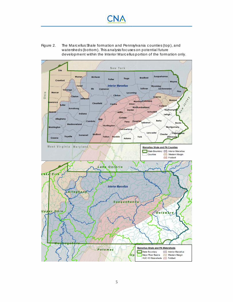
Figure 1. This analysis and environmental burdens, impacts, and outcomes. .... 3 Figure 2. The Marcellus Shale formation and Pennsylvania counties (top),

and watersheds (bottom). This analysis focuses on potential future development within the Interior Marcellus portion of the formation only. ................................................................................................. 5

Figure 3. Average number of wells drilled per well pad in the Marcellus Shale from 2005 to 2013. ............................................................................. 10

Figure 4. Resource categories for various gas-in-place estimates used in industry ............................................................................................................ 11

Figure 5. Pennsylvania statewide land cover impacts from natural gas development including land disturbance by initial land cover type and core forest loss due to land disturbance and core to edge forest transition due to fragmentation. .................................................... 22

Figure 6. Pennsylvania statewide population within 0.5 and 1 mile of current or projected Marcellus well pad locations at full development. .................................................................................................. 29

Figure 7. Cumulative NOx, VOC, and methane emissions from projected natural gas development over a 30-year build-out. ................................ 37

Figure 8. Pennsylvania annual statewide emissions from projected natural gas development activities ......................................................................... 39

Figure 9. Uncertainty in statewide Marcellus annual NOx emissions due to emissions factor used for natural gas gathering compressor stations. ........................................................................................................... 42

Figure 10. Estimates of per well water use by HUC-8 watershed............................ 46 Figure 11. Total water and wastewater impacts for Pennsylvania associated

with hydraulic fracturing of projected wells through full development of the Marcellus Shale. ......................................................... 48

ix

List of Tables

Table 1. Well Projections Map Index. ....................................................................... 13 Table 2. Land Cover Impacts Map Index. .................................................................. 23 Table 3. Land cover groupings by 2011 National Land Cover Dataset

classifications. ................................................................................................ 24 Table 4. Population Impacts Map Index.................................................................... 30 Table 5. Emissions factors used in this study to evaluate air quality

impacts from projected natural gas development ................................. 35 Table 6. Air Emissions Impact Map Index. ............................................................... 40 Table 7. Water and wastewater maps by metric and category. ........................... 49 Table 8. Water and Wastewater Impacts Map Index. ............................................. 50

x

Glossary

Abbreviations

DRB Delaware River Basin EIA Energy Information Administration EPA Environmental Protection Agency FEMA Federal Emergency Management Agency NLCD National Land Cover Dataset PA Pennsylvania PA DEP Pennsylvania Department of Environmental Protection USGS United States Geological Survey CH

4 methane (gas)

EUR Expected ultimate recovery HF, HVHF Hydraulic fracturing, High-volume hydraulic fracturing HUC Hydrologic Unit Code NOx Nitrogen oxides (including NO

2, NO

3)

TRR Technically recoverable resources UNGD Unconventional natural gas development VOC Volatile organic compound ac acres cf/ Bcf/ Tcf cubic feet / Billion cubic feet / Trillion cubic feet cfs cubic feet per second ft feet gal gallons gpd gallons per day mi miles mi2 square miles MG million gallons MGD/MGY million gallons per day / million gallons per year

xi

Key terms

brine/produced water

Wastewater recovered during gas production consisting of frac fluid and contaminants from the shale formation.

consumptive use The portion of water use for fracking that is not recovered from shale.

core forest Forest of high ecological value more than 100 meters from other land use types, or infrastructure such as roads

edge forest Forest adjacent to (less than 100 meters) other land use types, or infrastructure such as roads

flowback Wastewater consisting primarily of frac fluid recovered in the first few weeks after hydraulic fracturing

frac fluid Fluid composed of water, sand, and chemicals injected at high volume into wells during the hydraulic fracturing process in order fracture gas-bearing shale

gathering pipeline Type of pipeline used to move gas from producing wells to the gas transmission pipeline network

hydraulic fracturing The process used to open fissures in gas bearing rock (esp. shale) using high-pressure injection of liquid.

lateral The horizontal portion of the well drilled in the shale formation.

Maxent Maximum Entropy (geospatial analysis technique)

play Layer of rock of similar age/type that contain petroleum products such as natural gas

unconventional natural gas development

General term for the combination of industry practices and technologies (e.g., hydraulic fracturing, horizontal drilling, multiple wells per well pad) used to extract natural gas from shale formations such as the Marcellus

water withdrawal The portion of the water used for fracking that is withdrawn directly from surface water sources.

well pad The location from which wells are drilled

1

Introduction

Since 2007, Pennsylvania has become a major natural gas producing hub due to technology advances that have facilitated gas extraction from the Marcellus Shale play, which underlies portions of Pennsylvania, West Virginia, New York, Maryland, and Ohio. The unconventional natural gas development (UNGD) technology that has enabled this shift is high-volume hydraulic fracturing (HVHF) paired with horizontal drilling on well pads with multiple wells per pad. Hydraulic fracturing uses a high-volume injection of “frac” fluid (water, sand, and added chemicals) to fracture the shale formation, which generally holds gas tightly. Horizontal drilling has allowed each well to travel along the shale layer for several thousand feet, and the ability to drill multiple wells per well pad has increased the speed and efficiency of gas extraction. The net result is that the Marcellus play, which as recently as 2006 was a small player in gas production, now accounts for over 20 percent of total U.S. dry gas

production [1].

Unlike several declining shale plays in other parts of the country, the Marcellus Shale play still has a large portion of its reserves available, and can support continuing development [2]. The pace of development will largely be tied to economic factors. The price of natural gas has a significant effect on development activity, as demonstrated by the recent declines in drilling activity in 2015 due to low gas prices. So does the marginal cost of production, which varies regionally across the Marcellus by a factor of three or more [1]. Economic factors in Pennsylvania (such as workforce development) and the role of the natural gas industry in the Pennsylvania economy will also influence development going forward. Over the long term, these economic forces will significantly influence the pace and timing of development, but the ultimate determinant of the amount of gas that could be developed is set by the amount of gas reserves and the technology available to recover the gas (subject to

applicable restrictions and regulations pertaining to gas development).

According to the U.S. Energy Information Administration’s (EIA) estimates, the Marcellus Shale contains over 144 trillion cubic feet (Tcf) of technically recoverable reserves, of which over 65 Tcf are considered proven reserves [3], and of which most are in Pennsylvania. Over 11 Tcf has been produced in Pennsylvania through the end of 2014, and over 8,800 wells have already been drilled. Taken together, these statistics indicate that tens of thousands more wells would be needed to fully develop the Marcellus Shale resources in Pennsylvania.

2

Inevitably, UNGD results in some potential impacts to the environment across the landscape of development due to the activities needed to support the phases of development. Land must be cleared and developed in order to build the well pads, roads, and pipelines necessary to access the gas. During production, HVHF requires water to mix frac fluid, and produces volumes of wastewater along with gas that must be handled. Equipment that is necessary to run gas development operations (drilling rigs, pumps, trucks, compressors, and other equipment) produces air emissions, dust, and noise. All of these activities necessary for UNGD have impacts to land cover (including forests), watersheds, air, and human populations [4-22]. Some of these impacts can be mitigated more easily than others, and regulations, industry practices, and simple probability (large variations well-to-well) can have a large effect on the level of impact, or the risk of certain impacts occurring. The outcomes associated with these impacts are largely tied to the density and pace of natural gas development, and the underlying conditions and vulnerability of the affected areas’ resources. But in order to understand these impacts, it is first

necessary to understand the activities that cause them.

This analysis begins to answer the question: What happens if the Marcellus Shale is fully developed?

Understanding this report

We present this analysis as one projection of what the impacts of full development of the Marcellus Shale may look like across the landscape of Pennsylvania. This study is not intended to be a comprehensive examination of all potential impacts of gas development, but rather is meant to be a starting point and useful guide that can help identify impact categories where more in-depth analysis may be warranted. The

geographic breadth of this study limits the depth of the impact analysis.

Our methodology is relatively straightforward: Determine the number of wells required to fully develop the technically recoverable shale resources in the Interior Marcellus, and estimate the most likely well pad locations associated with this level of development. Then, using the projected numbers and locations of the wells and well pads, estimate the level of impacts using available data and scientific literature. In general, we multiply data on “per well pad” impact by projected number of well pads to estimate overall impact, and disaggregate results using useful geographic

delineations (counties and watershed boundaries).

The metrics used to evaluate the impacts of gas development can be most easily explained by using the Burdens > Impacts > Outcomes framework advanced by

Krupnick et al. [23] to discuss potential environmental impacts of fracking. Burdens are the numeric quantification of different activities that may have a potential impact. Impacts are the resulting effects of these activities on an environmental

3

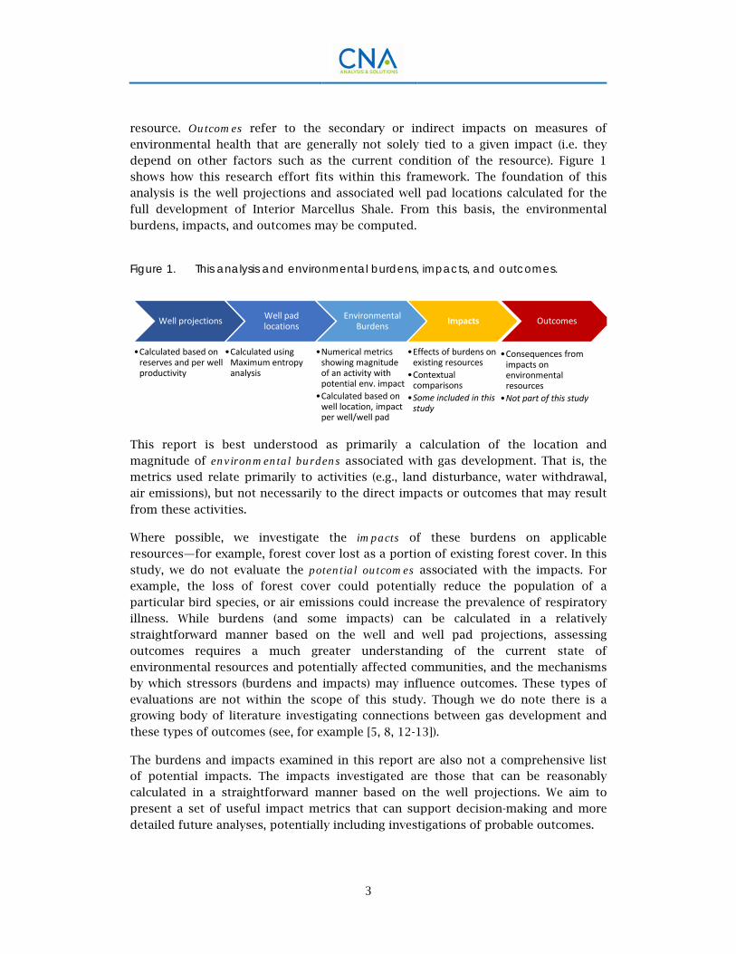
resource. Outcomes refer to the secondary or indirect impacts on measures of environmental health that are generally not solely tied to a given impact (i.e. they depend on other factors such as the current condition of the resource). Figure 1 shows how this research effort fits within this framework. The foundation of this analysis is the well projections and associated well pad locations calculated for the full development of Interior Marcellus Shale. From this basis, the environmental

burdens, impacts, and outcomes may be computed.

Figure 1. This analysis and environmental burdens, impacts, and outcomes.

This report is best understood as primarily a calculation of the location and magnitude of environmental burdens associated with gas development. That is, the metrics used relate primarily to activities (e.g., land disturbance, water withdrawal, air emissions), but not necessarily to the direct impacts or outcomes that may result

from these activities.

Where possible, we investigate the impacts of these burdens on applicable resources—for example, forest cover lost as a portion of existing forest cover. In this study, we do not evaluate the potential outcomes associated with the impacts. For example, the loss of forest cover could potentially reduce the population of a particular bird species, or air emissions could increase the prevalence of respiratory illness. While burdens (and some impacts) can be calculated in a relatively straightforward manner based on the well and well pad projections, assessing outcomes requires a much greater understanding of the current state of environmental resources and potentially affected communities, and the mechanisms by which stressors (burdens and impacts) may influence outcomes. These types of evaluations are not within the scope of this study. Though we do note there is a growing body of literature investigating connections between gas development and

these types of outcomes (see, for example [5, 8, 12-13]).

The burdens and impacts examined in this report are also not a comprehensive list of potential impacts. The impacts investigated are those that can be reasonably calculated in a straightforward manner based on the well projections. We aim to present a set of useful impact metrics that can support decision-making and more

detailed future analyses, potentially including investigations of probable outcomes.

Well projections

•Calculated based on reserves and per well productivity

Well pad locations

•Calculated using Maximum entropy analysis

Environmental Burdens

•Numerical metrics showing magnitude of an activity with potential env. impact

•Calculated based on well location, impact per well/well pad

Impacts

•Effects of burdens on existing resources

•Contextual comparisons

•Some included in this study

Outcomes

•Consequences from impacts on environmental resources

•Not part of this study

4

Specifically, we ask: What will be the approximate level of environmental burdens to land resources, forests, water, air, and the population of Pennsylvania that can be reasonably expected based on projections of the numbers of wells and well pads needed to fully develop the Marcellus Shale? We investigate particular impact metrics such as land area needed for infrastructure, forest and core forest loss, water withdrawals, wastewater generated, populations living in close proximity to wells, and air emissions. The impacts investigated tend to be those that can be reasonably estimated based on the well development numbers and locations using average per-well factors (from peer-reviewed literature or publicly available data sources), or additional geospatial analysis or modeling. In general, these impacts reflect average conditions for activities necessary for well development (e.g., building well pads,

water withdrawals to mix frac fluid, or running compressors to pump natural gas).

This analysis does not investigate some other potential impacts often associated with gas development, because of data limitations or difficulty assessing impacts at such a large spatial scale. Some impacts such as groundwater contamination (associated with well-casing failures, surface spills of wastewater fluids, etc.) are difficult to investigate because the probabilistic nature of the impact cannot be directly tied to well locations without overly simplistic assumptions. Other impacts such as wastewater treatment and discharge, and community impacts such as truck traffic cannot be investigated easily because they require knowing information about natural gas operations (e.g., wastewater disposal method and location, preferred routes) that cannot easily be determined for long-range projections of well development. Finally, some impacts such as erosion and pollutant loading impacts associated with land development are not investigated because the analysis required

is too complex and time-consuming to be completed at this geographic scale.

The primary output of this analysis is a series of maps displaying potential impact from a full development of the shale in several impact categories. We present the information in relevant geospatial context, recognizing that the impacts do vary considerably across Pennsylvania in relation to the relative intensity of gas development and existing condition of local resources. Specifically, we map the impacts by county or watershed (see Figure 2) depending on the nature of the impact. For instance, air emissions and population data are collected at the county level, while water withdrawal impacts are associated with watersheds. For mapping watershed impacts, we use Hydrologic Unit Code 10 (HUC-10) watershed boundaries from the United States’ Geological Survey’s (USGS’s) Watershed Boundary dataset. In

Pennsylvania, there about 330 HUC-10s, with an average size of 162 square miles.

The maps can be downloaded in sets corresponding to each chapter of this report at:

www.cna.org/PA-Marcellus.


5

Figure 2. The Marcellus Shale formation and Pennsylvania counties (top), and watersheds (bottom). This analysis focuses on potential future development within the Interior Marcellus portion of the formation only.

6


7

Projected Natural Gas Development

This chapter presents the current landscape of the Marcellus Shale play in order to predict how it may change in the future in response to the expansion of natural gas extraction. In particular, we focus on the potential development in the Interior Marcellus Shale Assessment Unit, since 95 percent of the shale’s reserves are estimated to fall within this boundary [24], and 98 percent of the new wells

developed in the region since 2011 have been within this boundary.3

For this report, we focused our analysis to determine where this development would most likely occur through Pennsylvania to realize full extraction of natural gas reserves. We then modeled the extent of potential infrastructure (gathering pipelines and access roads) necessary to support these well pads in the DRB. We did not assess impacts from additional infrastructure needed to support natural gas extraction that is not directly tied to individual well pads.4 Additionally, we did not assess other types of pipeline infrastructure (e.g., interstate and intrastate transmission pipelines, or intermediate collector pipelines to connect to several gathering pipelines) that may be developed beyond the gathering lines that bring the gas from the well pad to

the nearest connection to the existing pipeline network.

Methods, data sources, and assumptions

Well location modeling

To predict the most likely locations for the placement of future wells in Pennsylvania, we used the same approach as in our previous analysis of the Delaware River Basin [4], which is based on methodology employed by Johnson et al. (2010)

3 The other assessment units (Western Margin and Foldbelt) are generally thinner and less rich in gas. Additionally, there were not a sufficient number of existing wells in these areas to complete the geospatial analysis necessary for well location modeling.

4 For example, equipment storage sites, industrial wastewater treatment plants, centralized wastewater impoundments, quarries, water withdrawal sites, and other supporting infrastructure not associated with individual well pads.

8

[18]. Briefly, we combined geospatial analysis and maximum entropy (Maxent) modeling using historical well location data and geological and environmental data layers for the Marcellus Shale. This method produced a probability surface in which each pixel contained a value that denoted the likelihood for development. We then determined the projected well pads’ locations across the surface by using spatial averaging to center the locations on the highest Maxent value neighborhoods, and used exclusion distances to ensure adequate average well pad spacing.5 While a full description of the methodology can be found in our previous report [4], we present

below the assumptions, data sources, and updates that we used for this analysis:

• Well development will occur at eight wells per well pad on average, based on recent trends of development in the state. New well pads would be built to

accommodate each new set of wells. All wells drilled are horizontal wells.

• Development continues until all technically recoverable reserves for the Interior Marcellus (144 trillion cubic feet) are exhausted, at an estimate of 1.9 Billion cubic feet (Bcf) estimated ultimate recovery (EUR) per well. Both values are based on EIA estimates for the Marcellus Shale. We did not include development outside of the Interior Marcellus (e.g., in the Foldbelt or Western

Margin Marcellus) or in other shale plays such as the Utica.

• For this analysis, “build-out” or “full development” are terms that refer to the condition when the EIA estimate of technically recoverable reserves in the Interior Marcellus play has been exhausted. We assume that build-out will occur over 30 years. We do not explicitly factor in economics (natural gas price projections, costs of development, etc.) in determining extent of

development.

• Well spacing was based on an average lateral length of 5,000 feet and lateral spacing of 600 feet with eight horizontal wells per well pad, consistent with

average Marcellus wells in 2014 [26].

• Well pad location exclusions followed PA regulations [27]:

o Buildings — 500 ft (GIS address points [28]);

o Streams and Wetlands — 300 ft; (NHDPlus v2 flowlines, NHDPlus v2

waterbodies [29]);

o Outside 100-year floodplains (FEMA flood hazard layer [30]);

5 This methodology differs from that of a previous analysis [25], which used fixed or grid spacing for estimating well pad locations. The spatial averaging of Maxent values helps place the well pad in the center of a favorable development zone.

9

o Protected areas (USGS Gap Analysis Program Protected Areas

Database, class 1 and 2 [31]).

• UNGD development with HVHF is not currently permitted in the portion of Pennsylvania within the Delaware River Basin (primarily affecting Wayne and Pike counties). For this analysis, we assumed that development would be permitted in this area, in order to analyze potential impacts to the Delaware

River Basin.

Key parameters

The projections of the ultimate number of wells and well pads across the Marcellus are sensitive to several key assumptions. Notably, the number of wells per well pad, the estimated EUR per well, overall reserves estimate, and the number of horizontal versus vertical or directional wells drilled all affect the overall well numbers. Average well pad spacing (a function of lateral length and wells per pad), and exclusion areas will impact well locations. We also assume that all future well development will use HVHF with horizontally drilled wells. Although vertical and directional wells are still drilled in the Marcellus, nearly all new Marcellus wells in Pennsylvania are drilled

with horizontal drilling [2].

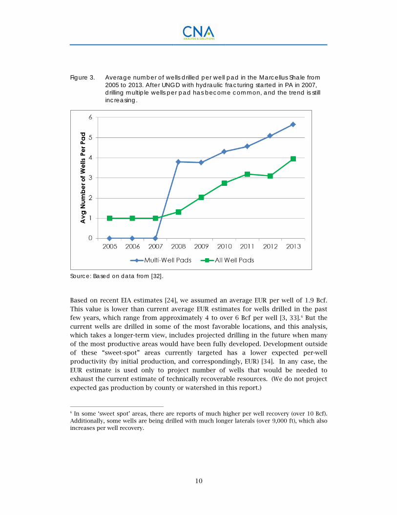
We used an assumption of eight wells per well pad on average as reflective of typical development practice over the time horizon of this study (roughly 30 years). This is higher than the current average, but there is a clear upward trend in both the number of well pads with multiple well drilling, and the number of wells drilled on multi-well pads [32]. Also, recent analysis has found that nearly all new development is completed with multiple wells per pad [2]. Figure 3 presents the trend of well pad development in the Marcellus Shale and shows that the average number of wells on a multi-well pad has increased from fewer than three wells per pad in 2008 to almost six wells per pad in 2013. Further, there are already instances of well pads with 16 or more wells drilled. The number of wells per pad can have a significant influence on the level of impacts for several impact categories (e.g., land disturbance, forest fragmentation, population affected), and less influence for others (e.g., water withdrawal, air emissions). With more wells per pad, fewer well pads get developed across the landscape, given the same total number of wells. Previous studies [4, 18]

have investigated how impacts differ depending on the number of wells per pad.

10

Figure 3. Average number of wells drilled per well pad in the Marcellus Shale from 2005 to 2013. After UNGD with hydraulic fracturing started in PA in 2007, drilling multiple wells per pad has become common, and the trend is still increasing.

Source: Based on data from [32].

Based on recent EIA estimates [24], we assumed an average EUR per well of 1.9 Bcf. This value is lower than current average EUR estimates for wells drilled in the past few years, which range from approximately 4 to over 6 Bcf per well [3, 33].6 But the current wells are drilled in some of the most favorable locations, and this analysis, which takes a longer-term view, includes projected drilling in the future when many of the most productive areas would have been fully developed. Development outside of these “sweet-spot” areas currently targeted has a lower expected per-well productivity (by initial production, and correspondingly, EUR) [34]. In any case, the EUR estimate is used only to project number of wells that would be needed to exhaust the current estimate of technically recoverable resources. (We do not project

expected gas production by county or watershed in this report.)

6 In some ‘sweet spot’ areas, there are reports of much higher per well recovery (over 10 Bcf). Additionally, some wells are being drilled with much longer laterals (over 9,000 ft), which also increases per well recovery.

11

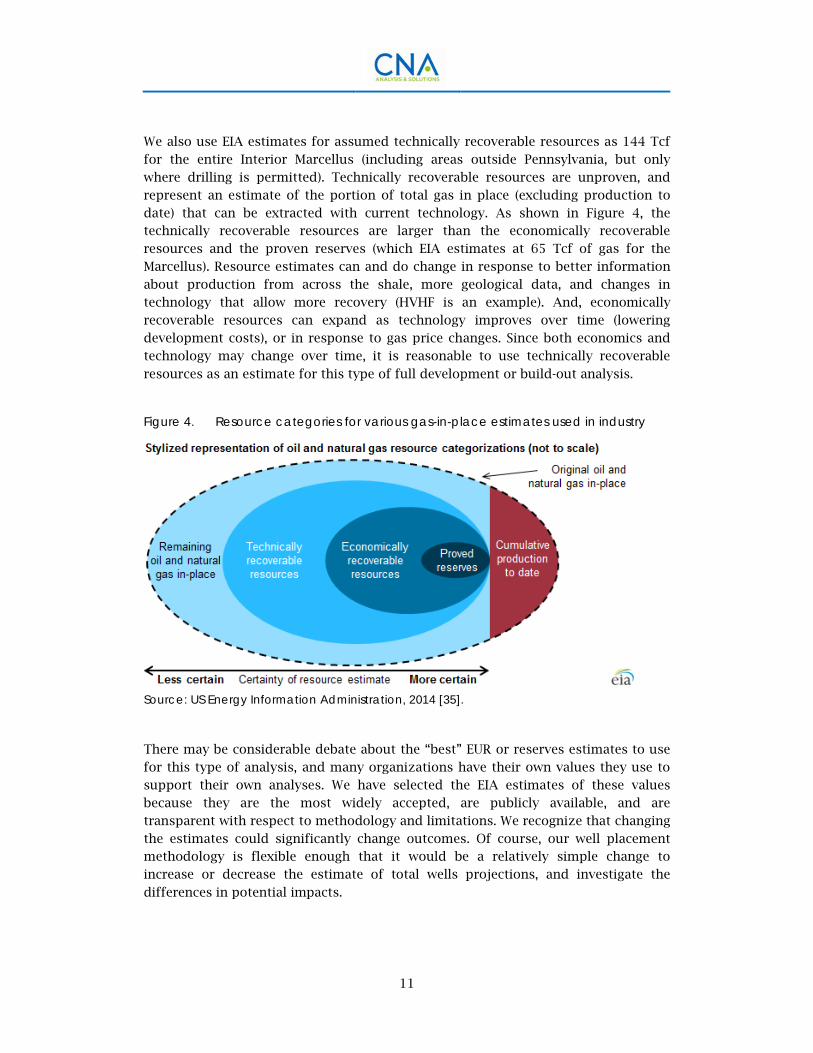
We also use EIA estimates for assumed technically recoverable resources as 144 Tcf for the entire Interior Marcellus (including areas outside Pennsylvania, but only where drilling is permitted). Technically recoverable resources are unproven, and represent an estimate of the portion of total gas in place (excluding production to date) that can be extracted with current technology. As shown in Figure 4, the technically recoverable resources are larger than the economically recoverable resources and the proven reserves (which EIA estimates at 65 Tcf of gas for the Marcellus). Resource estimates can and do change in response to better information about production from across the shale, more geological data, and changes in technology that allow more recovery (HVHF is an example). And, economically recoverable resources can expand as technology improves over time (lowering development costs), or in response to gas price changes. Since both economics and technology may change over time, it is reasonable to use technically recoverable

resources as an estimate for this type of full development or build-out analysis.

Figure 4. Resource categories for various gas-in-place estimates used in industry

Source: US Energy Information Administration, 2014 [35].

There may be considerable debate about the “best” EUR or reserves estimates to use for this type of analysis, and many organizations have their own values they use to support their own analyses. We have selected the EIA estimates of these values because they are the most widely accepted, are publicly available, and are transparent with respect to methodology and limitations. We recognize that changing the estimates could significantly change outcomes. Of course, our well placement methodology is flexible enough that it would be a relatively simple change to increase or decrease the estimate of total wells projections, and investigate the

differences in potential impacts.

12

Infrastructure modeling

In addition to well pads, we considered other natural gas infrastructure required to support development, which at a minimum includes roads to move equipment and materials to and from the well pad, and gathering pipelines which move gas produced at the well pad to market. To model the roads and gathering lines, we used the least-cost path-optimization approach, which is a common approach for siting and analyzing linear infrastructure. This methodology was used in our earlier study of the DRB, and we provide further detail in that report. [4] Briefly, to perform this modeling, we first developed a cost surface for Pennsylvania by combining a variety of geospatial layers7 relevant to routing, and assigning a cost to the values associated with each layer. We used this cost surface with the “Least Cost Path” tool in ArcGIS 10.2 to determine the most efficient route from each of the projected well pads to

the existing infrastructure.8

Results

Based on the EIA estimate of technically recoverable resources divided by the EIA average total production per well, and subtracting the number of existing Marcellus wells, we get the number of new wells expected, which is over 66,000 for the entire Interior Marcellus. In our modeling, Pennsylvania accounts for 72 percent of these expected wells (47,600). Based on a scenario of 8 wells per pads, this amounts to 5,950 well pads that may be developed throughout the Commonwealth to accommodate these new wells.

Based on our infrastructure modeling, we found that 5,832 miles of gathering pipeline and 1,342 miles of road would be developed to support full build-out of the Marcellus Shale in Pennsylvania based on our projections of well pad locations. The infrastructure modeled only includes roads/pipelines needed to connect well pads to

7 These geospatial layers, including slope, land use, roadways, streams, floodplains, and protected lands, are used in least-cost optimization to reflect the relative difficulty of building infrastructure through or across these landscape features. For example, building on flat land is easier than building on steep slopes, and crossing wetlands is more difficult than crossing pastures. In general, the least-cost “path” will be the most efficient path to minimize distance while avoiding terrain features that are difficult to cross.

8 We modeled the least-cost path for each well pad independently, but in (the many) cases where pipeline or road infrastructure followed the same path, we assumed they could share a road/pipeline (i.e., we did not double count this length). Modeling the infrastructure build-out in sequence, well pad by well pad, or centralized planning of intermediate collector lines could result in slightly lower distances per well pad, but likely would not change results significantly.

13

the nearest (or least costly to reach) point in the existing road or pipeline network. The analysis does not consider additional infrastructure needed to support increasing gas production on regional or statewide basis such as interstate or intrastate gas transmission pipelines. Note that these projections are intended to illustrate the potential scale of infrastructure with a reasonable estimation of spatial extent and are not meant to predict exact locations.

We have developed a variety of maps to present the statewide results of projected natural gas development, in order to provide spatial context for our discussions. Table 1 gives an overview of these maps. The discussion section provides

descriptions and information that will help readers understand each map.

Table 1. Well Projections Map Index. Access maps at www.cna.org/PA-Marcellus

Map Title 1.1 Probability surface for well pad development in the Interior Marcellus 1.2 Projected well pad development locations 1.3 Projected well development by county 1.4 Projected well development by watershed 1.5 Projected well development density 1.6 Projected natural gas infrastructure by county

Discussion

Map 1.1 – Probability surface for well pad development in the Interior Marcellus

This map shows the probability surface generated by the Maxent program based on existing well locations, and ‘environmental variables’ including shale characteristics, existing infrastructure, land use, and terrain. The surface has 30-meter resolution and uses a color scheme to depict the relative likelihood of development (i.e., Maxent value) based on the environmental variables, with “cooler” colors denoting areas with a lower probability of development, and “warmer” colors denoting those with a higher probability of development. These probabilities are based on the characteristics of the underlying geospatial layers at existing Marcellus wells developed from 2007 to 2013. The Maxent surface was developed for the Interior Marcellus play only. We have also included the boundaries of the full extent of the Marcellus formation. These boundaries will be included in all maps generated from this analysis for spatial context. The two major hotspots for existing drilling are in

the southwest and northeast portions of the Marcellus Shale in Pennsylvania.


14

Map 1.2 – Projected well pad development locations

This map shows the location of projected additional well pads that would be developed in the Pennsylvania portion of the Interior Marcellus Shale through full development of EIA technically recoverable resources. We determined the projected well pad locations from the probability surface by using spatial averaging to center the locations on high Maxent value “neighborhoods” instead of particular individual pixels with high probability scores. The 5,950 well pads are divided into color-coded quintiles based on their Maxent value, to illustrate the relative suitability of each location. The existing Marcellus wells in the state are also depicted on the map, in grey, for reference.

Map 1.3 – Projected well development by county

This map shows the number of projected additional wells that would be developed in the Pennsylvania portion of the Interior Marcellus Shale through build-out by county. We developed well projections based on the projected well pad locations (see Map 1.2) with an average of eight wells per pad. The bars show the number of horizontally drilled to date, and then the projected number of additional wells broken into five groups (quintiles) ranging from most likely (red) to least likely (blue) as determined from the Maxent probability score.

Map 1.4 – Projected well development by watershed

This map shows the number of projected additional wells that would be developed in the Pennsylvania portion of the Interior Marcellus Shale through build-out by HUC10 watershed. We developed well projections based on the projected well pad locations (see Map 1.2) with an average of eight wells per pad.

Map 1.5 – Projected well development density

This map, like Map 1.4, shows the number of additional wells to be developed in each watershed based on the projections in this study. In this case, the map shading shows the additional wells normalized to watershed area in terms of wells per square mile. This map shows the relative density of well development independent of watershed size. (Large watersheds can accommodate more well pads, which might skew the perception of where development is most intense, absent this correction.)

15

Map 1.6 – Projected natural gas infrastructure by county

This map shows the amount of projected road and gathering pipeline infrastructure, in miles, that would be developed in Pennsylvania to support natural gas development to build-out. We used least-cost path optimization to model the gathering pipelines and access roads that could be developed to connect the projected well pads to existing infrastructure in the state. The map includes the existing pipeline infrastructure in the state, in red, for reference and context (the existing road infrastructure is too dense to provide meaningful information). Within each county, we also present the average miles of infrastructure developed to support a well pad in the county, which is a function of the proximity or density of existing infrastructure. The values show first the average miles of pipeline per well

pad, and then the average miles of road per well pad.

General discussion

To begin the study, we examined potential well development across the full extent of the Interior Marcellus. Evaluation of the probability surface shows two distinct areas with a concentrated high probability of development: one in the northeast region of Pennsylvania (around Tioga, Bradford, and Susquehanna counties), and the other in the southwest region of the state (around the Pittsburgh area). These two areas are consistent with a majority of the existing shale gas development seen in the Marcellus region. There are several other smaller hotspots, and large regions with

somewhat lower potential for development.

The probability surface and well projection estimates are subject to several important caveats. By necessity, the reserves estimates represent a snapshot in time; they are constantly changing based on new information collected from drilling productivity and geological review. It is likely these estimates will continue to change, but we have elected to use the most recent EIA data available at the time of the study. Since this a long-range analysis, we also assume no regulatory constraints (other than those listed in the methods section)9 or economic constraints when

developing the probability surface.

Our projections show that 12 counties could each see development of over 2,000 new wells to support full extraction of the resources in the Interior Marcellus. Many of these counties are located within the current hot spots, but a few, such as Potter,

9 For example, this analysis does allow development in the Delaware River Basin, and in state forests, which are locations that currently have moratoriums on new development.

16

Elk, and Armstrong counties, are not experiencing as much development today and thus would see larger increases in development, albeit possibly not until the current hot-spots are nearly fully developed. Even with the updated assumptions used in the modeling for this analysis, it is worth noting that our results for Wayne County (2,328 potential wells) are still very consistent with those from our previous analysis (2,424 potential wells) that focused on the Delaware River Basin.

We project well pad locations to support the calculation of impacts, but they should not be interpreted as explicit predictions of where wells will actually go. Although high-resolution spatial data allows fairly precise well pad siting, this analysis is most useful for identifying which portions of the Marcellus Shale may be most suitable for development (relative to all the others). Actual locations of wells depend on many site-specific factors, not the least of which is a legal lease contract to perform drilling on a property. Furthermore, the projected well pad locations should not be used to estimate impacts at small scales, such as for individual parcels or neighborhoods. Further, our modeling of the natural gas infrastructure was based on a standard GIS approach to provide a representative picture of this development, and carries the same caveat as the well pad locations. The actual routes could depend on additional

site-specific factors, such as lease holds and applicable laws and regulations.

We found that the average length of pipeline developed to support well pads varied widely across the state, owing to the extent of existing infrastructure in place. Counties in northeast Pennsylvania showed an average length of about 1.5 miles of pipeline per pad, which is consistent with previous studies on pipeline development [36-37]. However, the counties in the southwestern part of the state showed much lower averages of a half-mile or less per pipeline. Examination of the existing pipeline infrastructure supports these results, as the pipeline network is much denser in southwest Pennsylvania, reducing average distance needed to connect to it. This produced a statewide average of pipeline length per pad of around 1 mile. The average length of road per well pad was much more consistent across the state, not deviating much from about 0.2 miles per pad, likely owing to the dense network of

road infrastructure already in place.

Of course, there are several caveats to keep in mind related to the infrastructure modeling. The infrastructure modeled only includes the well pads, gathering pipelines, and roads that are necessary, at minimum, for unconventional gas development. In the next section, land cover impacts are limited to these infrastructure types, and do not include other facilities such as equipment storage, or centralized waste processing facilities. The routes selected by the least cost path analysis do not consider the suitability of the existing roads or pipelines for handling the traffic or gas volume from the new wells. Rather they consider the most efficient route to the nearest (or least costly to reach) existing road or pipeline. A longer path could be necessary if there are access, capacity, or usage issues with the nearest road/pipeline. Also note that the roads and especially pipeline data may not be

17

completely up to date if they are available at all [38], so shorter paths could exist in areas that have had recent road or pipeline construction. Finally, planning pipeline or road layouts for several well pads at a time (if a single company operated them, for instance) could result in different infrastructure development patterns (total length

could be shorter or longer).

In general, our estimates for gathering pipeline length are lower than some other estimates such as the 25,000 miles estimated by former PA Department of Environmental Protection (DEP) secretary John Quigley [38], or the 10,000 miles estimated by the Nature Conservancy for a similar number of well pads (based on an average of 1.65 miles per well pad) [36]. One potential explanation is that our infrastructure modeling reflects regional differences in existing pipeline density. Further, the other estimates may include some other intermediate gathering and

transmission pipeline infrastructure beyond the immediate gathering pipelines.

There are several ways this analysis could be revised and extended in the future. The maximum entropy analysis in particular is flexible, and can be updated to include more recent data, and additional data layers not included in this study. Simply repeating the analysis will a larger set of existing wells to ‘seed’ the model should result in improved projections. Similarly, updated maps of underlying layers such as gas pipeline infrastructure, and roads could affect the relative probability of development where there has been rapid change in the past few years.

There are several possibilities for other data layers to include in the maximum entropy modeling. As more Marcellus wells are drilled, improved maps of shale richness (e.g., total gas in place) and well productivity are being generated by the gas industry and academics. These could be helpful to add additional weight to development in known hot-spots. We did not include such maps as a data input to the maximum entropy analysis, as there was no authoritative data source, the maps available (e.g., investor presentations from the gas industry) vary widely in their estimates, and the geospatial data sets are either not publicly accessibly or not well-documented. We also did not consider the presence of other shale plays in the region (e.g., the Utica), but it is likely the ability to access multiple plays influences the likelihood of drilling. Finally, leasehold data could be included in the maximum entropy analysis to identify areas with particular likelihood for drilling.

While these data sets could improve the projections, we intentionally limited the maximum entropy analysis to layers reflecting physical parameters of the shale, land surface, and infrastructure that are publicly available and not subject to rapid change.

In general, the marginal information gained for Maxent analysis decreases as more input layers are added. As the available data sets improve, and become more widely accessible, these additional factors plus economic and regulatory considerations

could be explicitly included in follow-on studies.

18


19

Impact on Land Cover

When assessing the environmental impacts of natural gas development, one of the most unavoidable aspects of such development is the impact on land cover. A typical well pad may cover three to five acres of land to support the well-drilling and hydraulic process, which includes the well site and room for supporting equipment, onsite water and wastewater storage (impoundments and/or closed tanks), and adjacent disturbed areas (e.g., land for regrading and leveling the well pad). In addition to the well pad, development of land to support natural gas extraction requires access roads to the site and gathering or feeder pipelines to transport the extracted gas from the site to the existing transmission infrastructure [14, 36-37, 39]. The resulting land disturbance from this development can present both short- and long-term risks to the use of the land, depending on the remediation and reclamation

procedures used [40-41].

One issue associated with the development activities from natural gas extraction in the Marcellus Shale is the impact on forests [14, 18, 39-40]. Pennsylvania’s dense forest cover provides the region with a variety of ecosystem services, such as carbon sequestration, clean air, aquifer recharge, and recreation/eco-tourism [42]. Furthermore, forest cover in the region is home to a variety of different plant and animal species that rely on the forest for their habitat. The edge transition from non-forest to forest area creates a habitat that tends to favor generalist species over rare or vulnerable species, and an increase of edge forest can promote the spread of invasive species [40].

Another issue of interest focuses on the relationship between land and water. Clearing of forests and other natural land cover for natural gas infrastructure and subsequent conversion to impervious cover or compaction of soil in construction right-of-way can change the hydrologic behavior of the landscape, leading to more runoff and erosion and less groundwater infiltration. Impervious cover (or more broadly, changes in the perviousness of the landscape) can be used to assess impacts on water quality, since it represents how much water can infiltrate the soil versus how much will run off into nearby streams [43]. Stream quality in a watershed will generally become impacted once impervious cover reaches above 10 percent, though some studies have shown impacts to streams above as little as 2 percent [44]. Stream crossings by road and pipeline infrastructure can also have an impact on flow characteristics in the stream, sediment loads, and water quality, and on the health

and movement of aquatic species [45-48].

20

To assess the potential impacts of natural gas development on land cover in Pennsylvania, we combined our projections of natural gas well and infrastructure development in the state with a suite of GIS tools and methodology. We used the projected well pad locations and supporting infrastructure to survey the impacts to current land cover, and the potential for forest fragmentation. Then, to give context to the amount of area impacted, we compared the total disturbance area to the

amount of existing developed land.


Before the infrastructure to support natural gas extraction—e.g., well pads, gathering pipelines, and access roads—can be constructed, the land must be cleared. In the previous chapter, we documented how the natural gas infrastructure locations were modeled as points for well pads, and linear features for roads and pipelines. To determine the land area affected by disturbance from these activities, we used the “Buffer” tool in ArcGIS to map the spatial extent of the well pads and pipeline and

road rights-of-way.

We then used this footprint to extract the impacted land cover values from the 2011 National Land Cover Dataset (NLCD) raster. “Land disturbance” refers to all land that falls within this footprint. By contrast, for the purpose of this study, “new clearing” refers to all land cover types within this footprint except for developed land (open space, low density, medium density, or high density), which has already been cleared. For this analysis, we considered the land necessary for initial development of the infrastructure including the construction rights-of-way necessary for equipment

access to build the roads and pipelines.

Given the prevalence of forest cover in Pennsylvania (approximately 60 percent of total land cover) and the potential for impact, we extended our land cover analysis to focus on the extent of potential forest fragmentation caused by this disturbance. To assess this impact, we generated a baseline core forest raster from the NLCD raster using the Landscape Fragmentation Tool v2.0 [49] and applied a forest edge width of 100 meters. After we generated the baseline condition, we assessed the potential impact from natural gas development by applying an additional 100-meter buffer to the projected spatial footprint of gas infrastructure (i.e., well pads and road and pipeline rights-of-way) to determine the changes in core and edge forest due to new

edge effects.

We also performed an analysis to compare the total new land cleared for gas infrastructure to existing developed land, in order to put the area of development into context. We estimated existing developed area from 2011 NLCD by computing the total of the developed land cover categories for low-, medium-, and high-density

21

development (NLCD codes 22, 23, and 24), which represent most urban and suburban

development areas (though not transportation or open cleared land).

To evaluate land cover burdens associated with Marcellus gas infrastructure

development, we used the following assumptions:

• Each well must be located on a well pad, and each well pad must be connected via road to an existing road, and via gathering pipeline to the existing natural gas pipeline network in PA (exclusive of distribution or “downstream” pipelines that bring natural gas directly to homes and

businesses).

• Each well pad occupies 3.5 acres.

• Each gathering pipeline requires a 30-meter right-of-way, and each access

road requires a 10-meter right-of-way.

• Core forest represents forest patches that lie 100 meters inward from the

nearest non-forest land cover (i.e., the forest edge).

• Potential new stream crossings were identified as intersection points between the modeled gathering pipeline and access road routes and Pennsylvania streams in the National Hydrography Dataset Plus version 2 (NHDPlus v2)

database [29].

The baseline results are presented using both the county and HUC10 watershed boundaries, but the impacts on forest and stream crossings are presented only for

watershed boundaries.

The assumptions for development area reflect the area generally needed for initial construction of infrastructure. After construction, some of this area may be partially returned to existing uses during operation, or at the conclusion of development. This report does not examine the evolution of the landscape through the development period as it responds to varying rates of development and varying remediation and reclamation practices. Instead, this report focuses on the direct area impacted by

construction of well pads, gathering pipelines and roads.

It is important to note that many of these infrastructure types do not cover the full range of land development activities associated with gas development, and they do not consider the estimates of additional area needed for equipment storage, centralized impoundments, wastewater treatment facilities, mining and quarry areas for soil/sand/gravel, earth moving (cut and fill) outside of the rights-of-way, landfill

areas, or other areas needed to otherwise support natural gas development.

22

Results

Based on our projections of well pad development and associated supporting infrastructure, we generated Pennsylvania-wide estimates of land cover burdens. Figure 5 shows the results of our analysis at the statewide level. We found that just under 95,000 acres of land could be disturbed by construction of natural gas infrastructure in the state, about 28,000 acres of which would constitute the clearing of forest cover. However, over 100,000 acres of core forest could be lost as a result of the combined effect of clearing and fragmentation due to the creation of new

forest edges.

These estimates are similar to, but slightly lower than previous Pennsylvania estimates of forest disturbance. The Pennsylvania Energy Impacts Assessment [18] completed by the Nature Conservancy found that for 60,000 wells, direct forest clearing would be between 38,000 acres (10 wells per pad) and 61,000 acres (six wells per pad). They estimated that additional core forest loss from fragmentation would

be between 91,000 acres (10 wells per pad) and 147,000 acres (six wells per pad).

Figure 5. Pennsylvania statewide land cover impacts from natural gas development including land disturbance by initial land cover type and core forest loss due to land disturbance and core to edge forest transition due to fragmentation.

While these figures are informative for comparisons to other shale gas basins or across industries, the importance of the impacts within Pennsylvania is difficult to

27,983 12,691

6,620

50,970

8,684

89,101

0

20,000

40,000

60,000

80,000

100,000

120,000

Land Disturbance Core Forest Loss

Impa

ct A

rea

(acr

es)

Forest - Core to Edge

Developed

Agriculture

Grassland/Wetland

Forest

23

discern from the statewide figures. For example, the 28,000 acres of forest cleared only represents 0.2 percent of the total forest cover in Pennsylvania. Breaking these impacts down to the county or HUC10 watershed level offers a more informative picture of where these impacts may be concentrated. Table 2 gives an overview of the maps generated for this impact category. The discussion section provides descriptions and useful information for understanding each map.

We also found that in many counties affected by natural gas development, the construction of new gas infrastructure could affect an area comparable to or larger than all existing developed land (e.g., residential, commercial, industrial land uses).10

Table 2. Land Cover Impacts Map Index. Access maps at www.cna.org/PA-Marcellus

Map Title 2.1 Land disturbance by county 2.2 Land disturbance by watershed 2.3 Forest cleared by watershed 2.4 Core forest loss by watershed 2.5 Existing developed area versus new clearing for gas infrastructure 2.6 Stream crossings by watershed

Discussion

Map 2.1 – Land disturbance by county

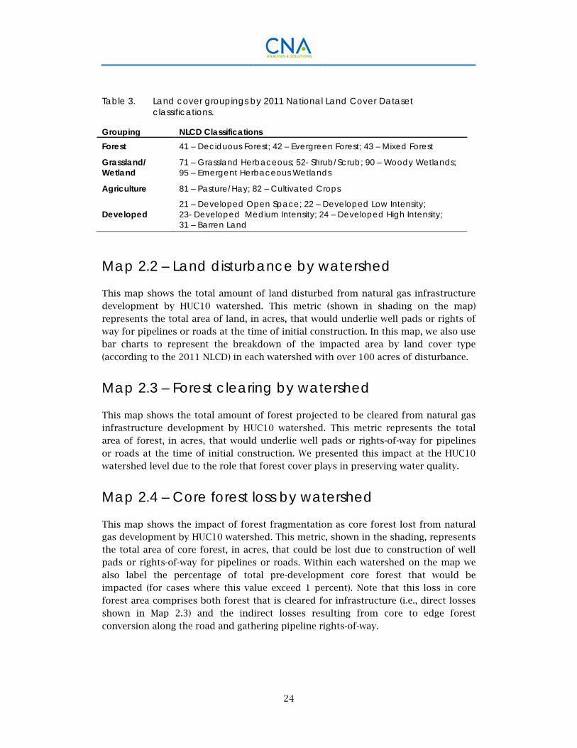
This map shows the total amount of land disturbed from natural gas development by county. This metric represents the total area of land, in acres, that would underlie well pads or rights of way for pipelines or roads. In this map, we use pie charts to represent the breakdown of the land cover impacted from natural gas development in each county. For visibility on the map, we combined the 11 land cover

classifications from the NCLD dataset into broader groups, as shown in Table 3.

10 We excluded Developed Open Space (NLCD code 21), which primarily includes undeveloped parcels and transportation.


24

Table 3. Land cover groupings by 2011 National Land Cover Dataset classifications.

Grouping NLCD Classifications Forest 41 – Deciduous Forest; 42 – Evergreen Forest; 43 – Mixed Forest

Grassland/ Wetland

71 – Grassland Herbaceous; 52- Shrub/Scrub; 90 – Woody Wetlands; 95 – Emergent Herbaceous Wetlands

Agriculture 81 – Pasture/Hay; 82 – Cultivated Crops

Developed 21 – Developed Open Space; 22 – Developed Low Intensity; 23- Developed Medium Intensity; 24 – Developed High Intensity; 31 – Barren Land

Map 2.2 – Land disturbance by watershed

This map shows the total amount of land disturbed from natural gas infrastructure development by HUC10 watershed. This metric (shown in shading on the map) represents the total area of land, in acres, that would underlie well pads or rights of way for pipelines or roads at the time of initial construction. In this map, we also use bar charts to represent the breakdown of the impacted area by land cover type

(according to the 2011 NLCD) in each watershed with over 100 acres of disturbance.

Map 2.3 – Forest clearing by watershed

This map shows the total amount of forest projected to be cleared from natural gas infrastructure development by HUC10 watershed. This metric represents the total area of forest, in acres, that would underlie well pads or rights-of-way for pipelines or roads at the time of initial construction. We presented this impact at the HUC10 watershed level due to the role that forest cover plays in preserving water quality.

Map 2.4 – Core forest loss by watershed

This map shows the impact of forest fragmentation as core forest lost from natural gas development by HUC10 watershed. This metric, shown in the shading, represents the total area of core forest, in acres, that could be lost due to construction of well pads or rights-of-way for pipelines or roads. Within each watershed on the map we also label the percentage of total pre-development core forest that would be impacted (for cases where this value exceed 1 percent). Note that this loss in core forest area comprises both forest that is cleared for infrastructure (i.e., direct losses shown in Map 2.3) and the indirect losses resulting from core to edge forest

conversion along the road and gathering pipeline rights-of-way.

25

Map 2.5 – Existing developed area versus new clearing for gas infrastructure construction

This map puts the land disturbance area associated with gas infrastructure development in context relative to total existing urban and suburban developed area by watershed. We computed the existing developed area in each watershed by summing the developed low-density, medium-density, and high-density land cover areas (NLCD codes 22, 23, 24) from the 2011 NLCD dataset. These estimates include most urban and suburban developed area in residential, commercial, and industrial land uses, but exclude most undeveloped open space and land use for transportation. The map compares the total land needed for initial construction of natural gas infrastructure with these existing developed areas.11 Yellow bars indicate the relative amount of land clearing for initial gas infrastructure construction by watersheds. The shading indicates the ratio of new gas infrastructure clearing area compared to existing developed area; a value of 1 indicates that the new infrastructure for gas development will occupy an area equal to all existing

development in the watershed.

Map 2.6 – Stream crossings by watershed

This map shows the projected number of new stream crossings associated with construction of road and pipeline infrastructure. Each stream crossing represents the intersection of the modeled gathering pipeline or road routes and streams in the USGS NHDPlus v2 database. Stream crossings within 250 feet of each other were treated as one crossing. On the map, the blue bars show the relative numbers of crossings by watershed, and the shading indicates the density of new stream crossings in units of crossings per 100 square miles. (The average watershed area of

162 square miles is on the same order of magnitude.)

General discussion

Our results showed that the construction of well pads and associated infrastructure to support shale gas development would have an impact on the land cover of Pennsylvania of over 100,000 acres, affecting primarily agricultural land (54 percent

11 This is purely to give context to the scale of impacted area on a watershed basis, and is not meant to imply that the land use types for gas infrastructure are similar in character to general urban/suburban development.

26

of disturbed land) and forest land (30 percent). This assessment of land disturbance only accounts for the well pad and rights-of-way for gathering pipelines and access roads to support those well pads. It does not account for additional construction that could occur to support natural gas development, such as new transmission pipelines that may be needed to help move gas to market, or new compressor stations to support gas transmission through the pipeline network. This construction could be expected to add to the footprint of development and cause additional land cover

impacts to the state.

Land-cover change from shale gas development is unavoidable, and disturbance can be significant at build-out. The loss of forest cover, in particular, can have significant impacts at the watershed level, such as degraded water quality and a loss of biodiversity from disappearing flora and fauna that cannot tolerate “edge effects.” For instance, we found that some Pennsylvania watersheds could lose over 5 percent of the existing core forest. Furthermore, remediation procedures to restore vegetation on the impacted land often do not replace mature forest cover, both because of the need to maintain access to gathering lines and use roads, and because

mature forests take a long time to grow.

Many of the environmental impacts and outcomes related to land cover changes are difficult to understand at this level of analysis because they are highly dependent on how the changes occur over time, something we did not investigate in this study. It is relevant to note that the land cover changes will not occur all at once, but build over

time as development continues. This analysis only considers total area within

Further study related to these impacts could include:

• Investigating effects of timing or rate of development and remediation and

reclamation practices used on land cover over time

• Estimating potential erosion and sediment loadings associated with land clearing and infrastructure development over time, subject to varying

assumptions of development rate and management practices

• Assessing vulnerability of species to the changes in forest area, loss of core

forests, or potential water quality effects.

27

Impact on Population

The distance from active well pads has been shown to correlate with certain health and environmental risk factors. Distance from activity is often used as a primary discriminator for determining dose intensity in public health studies. As a result, knowing the potential population within several distances of the proposed well pads is useful for evaluating potential impacts to Pennsylvania residents. In this study, we do not assess the likelihood of particular health outcomes occurring for populations

within the specified distances.

We report the populations living within two distances of well pads: one-half mile and one mile. These distances represent a close to moderate distance from well pads, and a moderate to farther distance, respectively. Several health studies have used similar distances to divide experimental groups when investigating variations in health risk

factors related to natural gas extraction [13, 19, 50-52].

The maps in this section should be read only as reporting the population (based on the 2010 Census) within the specified distances from well pads through full development of the Interior Marcellus play. These maps do not account for potential or projected population growth, or population living within the specified distance of other gas infrastructure such as roads, pipelines, equipment yards, compressor

stations, or wastewater treatment facilities.


We evaluate the population within two distances of Marcellus Shale well pads, one mile and one-half mile, using 2010 census block data for Pennsylvania [53]. Unlike our previous analysis for the DRB ([4]), which has a moratorium on natural gas development, there are existing Marcellus well pads in many parts of the Commonwealth. We analyzed the population within each county within the specified distance for “Current” Marcellus well pads, for “Additional” well pads developed

through build-out, and population “Outside” the specified distance.

We used a buffer method in ArcGIS to compute the areas within the specified distances, and intersected these areas with the Census population blocks to determine population affected. Our previous report, The Potential Environmental Impact from Fracking in the Delaware River Basin [4], has a full description of

28

methodology associated with computing the population living within a given distance of projected well pad locations. In brief, the following assumptions and data sources

were used.

• Population estimates were computed from 2010 census, census block data (2010 Census Bureau – SF1 data [53]), which is the finest resolution available. Population is assumed to be distributed with constant density within each census block to make population estimates where a portion of the census

block falls outside the designated distance from a well pad location.

• Existing well pad locations were computed based on commercially available

well location data (IHS, 2014 [54]) through September 2014.12

• Projected well pad locations from this analysis were used to determine “Additional” area. We only counted new area affected, and did not double-

count area within the specified distances of existing well pads.

• Total population estimates reflect the sum of “Current” and “Additional”

population within the designated distances.

Results

Based on the well pad locations generated for this analysis, and county-level data on population in U.S. census blocks, we estimated Pennsylvania-wide impact estimates for area and population within one-half and one mile of well pads. For area, we found 1,813 square miles within one-half mile of existing wells, and 6,354 square miles after all projected wells are included. The corresponding values are 4,680 and 14,450

square miles for the one-mile distance from well pads.

Figure 6 shows the Pennsylvania population estimated to be living within these

distances both currently and at our projection of full development.

12 Only wells designated as being drilled in the Marcellus play and having a status of “Active” or “Inactive” (not “Abandoned”) were used.

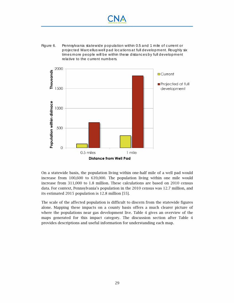
29

Figure 6. Pennsylvania statewide population within 0.5 and 1 mile of current or projected Marcellus well pad locations at full development. Roughly six times more people will be within these distances by full development relative to the current numbers.

On a statewide basis, the population living within one-half mile of a well pad would increase from 100,600 to 639,000. The population living within one mile would increase from 311,000 to 1.8 million. These calculations are based on 2010 census data. For context, Pennsylvania’s population in the 2010 census was 12.7 million, and

its estimated 2015 population is 12.8 million [55].

The scale of the affected population is difficult to discern from the statewide figures alone. Mapping these impacts on a county basis offers a much clearer picture of where the populations near gas development live. Table 4 gives an overview of the maps generated for this impact category. The discussion section after Table 4

provides descriptions and useful information for understanding each map.

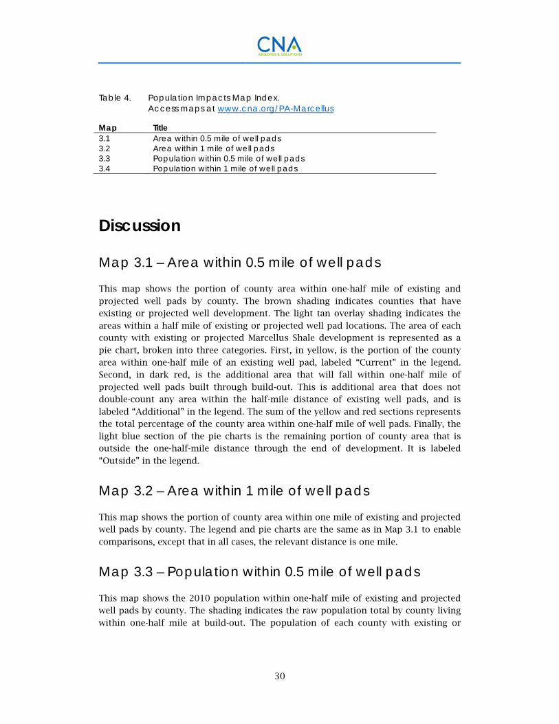
30

Table 4. Population Impacts Map Index. Access maps at www.cna.org/PA-Marcellus

Map Title 3.1 Area within 0.5 mile of well pads 3.2 Area within 1 mile of well pads 3.3 Population within 0.5 mile of well pads 3.4 Population within 1 mile of well pads

Discussion

Map 3.1 – Area within 0.5 mile of well pads

This map shows the portion of county area within one-half mile of existing and projected well pads by county. The brown shading indicates counties that have existing or projected well development. The light tan overlay shading indicates the areas within a half mile of existing or projected well pad locations. The area of each county with existing or projected Marcellus Shale development is represented as a pie chart, broken into three categories. First, in yellow, is the portion of the county area within one-half mile of an existing well pad, labeled “Current” in the legend. Second, in dark red, is the additional area that will fall within one-half mile of projected well pads built through build-out. This is additional area that does not double-count any area within the half-mile distance of existing well pads, and is labeled “Additional” in the legend. The sum of the yellow and red sections represents the total percentage of the county area within one-half mile of well pads. Finally, the light blue section of the pie charts is the remaining portion of county area that is outside the one-half-mile distance through the end of development. It is labeled

“Outside” in the legend.

Map 3.2 – Area within 1 mile of well pads

This map shows the portion of county area within one mile of existing and projected well pads by county. The legend and pie charts are the same as in Map 3.1 to enable

comparisons, except that in all cases, the relevant distance is one mile.

Map 3.3 – Population within 0.5 mile of well pads

This map shows the 2010 population within one-half mile of existing and projected well pads by county. The shading indicates the raw population total by county living within one-half mile at build-out. The population of each county with existing or


31

projected Marcellus Shale development is shown with a pie chart, indicating the percentage of the county population in three categories. First, in yellow, is the portion of the population living within one-half mile of an existing well pad, labeled “Current” in the legend. Second, in dark red, is the additional portion of the population that will fall within one-half mile of projected well pads built through build-out. This is “Additional” population, and does not double-count any population within the half-mile distance of existing well pads. Finally, the remaining portion of the population, shown in light blue, is that which is “Outside” of the one-half-mile

distance all the way through build-out condition.

Map 3.4 – Population within 1 mile of well pads

This map shows the 2010 population within one mile of existing and projected well pads by county. The shading by county is scaled identically to Map 3.3 in order to allow comparisons between the maps. The definitions for the pie chart are also the same as in Map 3.3, except that in all cases, the relevant distance is one mile instead

of one-half mile.

General discussion

These results present an estimate of population within certain radii of well pad locations. These population estimates are based on 2010 U.S. census data [53], and do not account for future population change. Further, this assessment only considers distance from well pads—the primary location for most natural gas development activity—and not other types of gas infrastructure.

This analysis is best interpreted as a way to understand the number of Pennsylvania residents that will experience natural gas development first-hand close to their residences. We can conclude that the number of Pennsylvania residents within these one-half-mile and one-mile radii of well pads will increase significantly—roughly six-

fold—over the population currently living within this proximity of existing well pads.

We also see regional patterns in the impacts on population. The largest such impacts in terms of pure numbers are in the southwest portion of the state, an area that already has significant existing gas development and, importantly, has a relatively high population density. By contrast, the counties in the northeast portion of the Commonwealth project tend to have most “coverage” of the county’s land area within the specified distances. For instance, in Map 3.1, almost all of Bradford, Susquehanna, Washington, Greene, and Armstrong counties could be within one mile of a well pad at some point during the development period. As a result, the portion of these county’s populations living within the specified distances is extremely high. Due to the lower population density of these counties, the raw total population

32

affected in the northeast portion of the state is lower than that in the southwest

region of Pennsylvania.

This information could be useful for several types of follow-on analysis, including economics and public health. In terms of economics, proximity to well pads may indicate how much of the population could be affected by economic impacts from

development (e.g., property value change, royalties).

While many studies show some correlation between distance from well pads and certain health risk factors, we did not attempt to connect these results to potential health impacts. Some potential follow-on health-related risk analyses could include, for example, potential groundwater contamination, or exposure to particular air pollutants. Or, public health studies could be used to estimate how incidence of certain health outcomes might change. We note that doing so would require a fuller, more detailed understanding of the specific nature of various gas development activities and facilities, and the intensity, duration, and frequency of potential health

risk stressors associated with each. .

33

Impact on Air Emissions

Unconventional natural gas development is an industrial process that involves a host of machinery and operations to extract natural gas from shale deposits. Shale gas operations release a variety of criteria pollutants that can degrade local air quality, including nitrogen oxides (NO

x); sulfur oxides (SO

x); particulate matter (PM); and

volatile organic compounds (VOCs), such as formaldehyde, benzene, toluene, ethylbenzene, and xylene (BTEX) [51-52, 56-58]. These emissions stem from diesel-powered equipment used for the well pad construction, drilling, hydraulic fracturing, and production processes. In addition, significant emissions can also arise from combustion-powered compressor stations that compress natural gas to keep it flowing through the pipeline system. Further, these activities could contribute to climate change due to greenhouse gas (GHG) emissions from shale gas development, which stem from the leakage of natural gas (i.e., methane, or CH

4) at various points

throughout the development cycle, from extraction to processing and transmission.

For this analysis, we calculated the potential contributions to NOx, VOC, and methane

emissions from projected natural gas development in Pennsylvania. We used the data from the Marcellus Shale Air Emissions Inventory [59] from the PA DEP to develop per-well emissions factors to apply to our projections. We also use DEP data to estimate the emissions contributions from additional compressor stations needed to support this development. We then present the emissions estimates from projected development at the county level across the state, along with the relative increase from emissions in the state today. We did not analyze the potential for any more

localized impacts on air quality, as this was beyond the scope of the study.


To assess the impacts to air quality, we applied relevant values from the PA DEP 2014 natural gas emissions inventory and professional literature to our build-out scenarios in order to calculate the emissions associated with natural gas development at the county level. We used an average development rate scenario to illustrate the impacts of development on air quality. This provides the average pace of development and shows the potential variation in emissions that could be expected from natural gas development activities in each county. We do note that in reality there would likely be considerable yearly variations in development per

34

county as operators focus on the more favorable locations first. We then developed a final year emissions estimate to represent the cumulative impact of ongoing emissions from natural gas production and the compression needed in order to bring

it to market.

To estimate the number of new compressor stations required to support our projected natural gas development, we used a data extract from the PA DEP listing of the midstream compressor stations in their 2014 inventory [59]. This extract included 509 facilities, which, PA DEP explained, included both gathering and transmission compressor stations. We used GIS analysis to classify any stations within 0.1 mile of a transmission pipeline as a transmission station and eliminate it from the list. This resulted in 320 gathering stations, or 1 compressor station for about every 9 well pads in Pennsylvania. Applying this ratio to our well pad projections, we estimate that 661 compressor stations will be developed to support

natural gas development.

We developed emission factors to apply to our projected natural gas development based on either the 2014 PA DEP natural gas emissions inventory or values from scientific literature. We classified development into three phases: pre-production, production, and gathering. Table 5 shows the emissions factors for NOx, VOC, and methane for each of these phases. Pre-production represents the emissions from drilling, hydraulic fracturing, and completion of the well. We developed this factor using the reported emissions from “drill rigs” and “completions” in the natural gas emissions inventory. Production represents the ongoing production of natural gas from the well. We developed this factor for NOx and VOC based on the study by Livovitz et al. [60]. For methane emissions, we used a recent study by Goetz et al. [61]. Finally, gathering represents the collection of natural gas from multiple well pads and compression of this gas to deliver it to transmission pipelines. We developed this factor based on the average emissions from the gathering stations in the seven counties within Pennsylvania that are most representative of UNGD: Bradford, Butler Greene, Lycoming, Susquehanna, Tioga, and Washington. These counties contain 75 percent of the UNGD in Pennsylvania through 2014, and would be most representative of the facilities used to support development moving

forward.

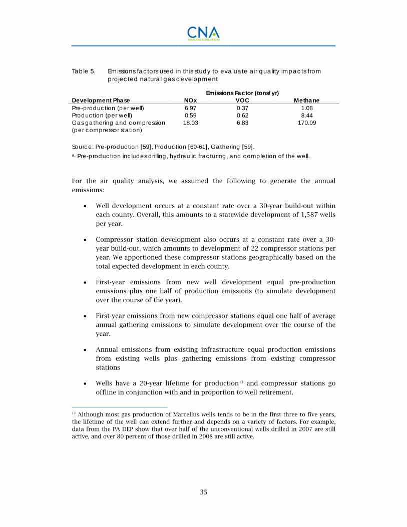
35

Table 5. Emissions factors used in this study to evaluate air quality impacts from projected natural gas development

Emissions Factor (tons/yr) Development Phase NOx VOC Methane Pre-production (per well) 6.97 0.37 1.08 Production (per well) 0.59 0.62 8.44 Gas gathering and compression (per compressor station)

18.03 6.83 170.09

Source: Pre-production [59], Production [60-61], Gathering [59]. a. Pre-production includes drilling, hydraulic fracturing, and completion of the well.

For the air quality analysis, we assumed the following to generate the annual

emissions:

• Well development occurs at a constant rate over a 30-year build-out withineach county. Overall, this amounts to a statewide development of 1,587 wells

per year.

• Compressor station development also occurs at a constant rate over a 30-year build-out, which amounts to development of 22 compressor stations peryear. We apportioned these compressor stations geographically based on the

total expected development in each county.

• First-year emissions from new well development equal pre-productionemissions plus one half of production emissions (to simulate development

over the course of the year).

• First-year emissions from new compressor stations equal one half of averageannual gathering emissions to simulate development over the course of theyear.

• Annual emissions from existing infrastructure equal production emissionsfrom existing wells plus gathering emissions from existing compressorstations

• Wells have a 20-year lifetime for production13 and compressor stations go

offline in conjunction with and in proportion to well retirement.

13 Although most gas production of Marcellus wells tends to be in the first three to five years, the lifetime of the well can extend further and depends on a variety of factors. For example, data from the PA DEP show that over half of the unconventional wells drilled in 2007 are still active, and over 80 percent of those drilled in 2008 are still active.

36

• Total annual emissions equal pre-production plus production plus gathering

and compression emissions.

Results

Using our projections of wells and compressor stations, we generated estimates of annual emissions of NOx, VOC, and methane from projected natural gas development in Pennsylvania. The contributions to these emissions from the different phases of natural gas development will change over time, as shown in Figure 7. Based on our 30-year build-out scenario, the pre-production phase contributes the majority of NOx emissions for the first 12 years, after which emissions from the production phase become the primary contributor. However, the pre-production phase contributes very little to the overall VOC and methane emissions from development. These graphs also illustrate the cumulative impact that ongoing emissions from production and gathering contribute to overall emissions

from development.

We find that given constant development rate, emissions tend to “peak” and plateau for several years. We use these “peak” annual emissions rates as the primary metric for mapping analysis, as they reflect the highest combination of pre-production,

production and gathering emissions during the development period.14

14 This peak will likely be lower than true peak emissions during the development period, as yearly development will not occur at a constant rate. Individual county peaks may be even higher if development is particularly concentrated over a short time period.

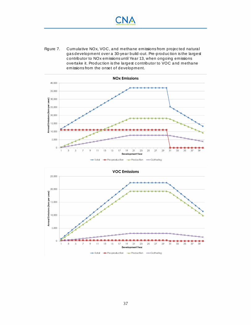
37

Figure 7. Cumulative NOx, VOC, and methane emissions from projected natural gas development over a 30-year build-out. Pre-production is the largest contributor to NOx emissions until Year 13, when ongoing emissions overtake it. Production is the largest contributor to VOC and methane emissions from the onset of development.

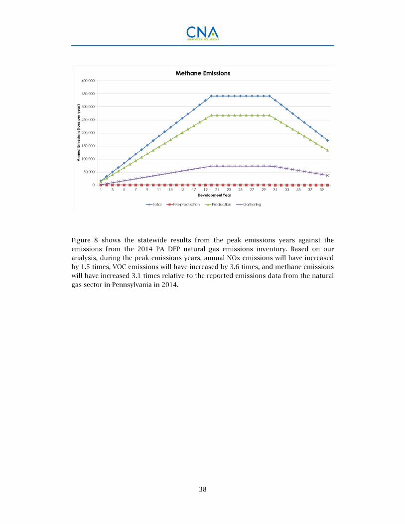
38

Figure 8 shows the statewide results from the peak emissions years against the emissions from the 2014 PA DEP natural gas emissions inventory. Based on our analysis, during the peak emissions years, annual NOx emissions will have increased by 1.5 times, VOC emissions will have increased by 3.6 times, and methane emissions will have increased 3.1 times relative to the reported emissions data from the natural

gas sector in Pennsylvania in 2014.

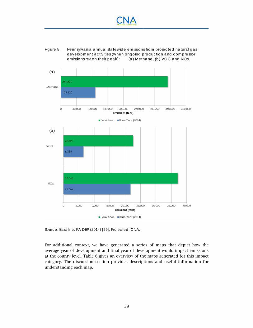
39

Figure 8. Pennsylvania annual statewide emissions from projected natural gas development activities (when ongoing production and compressor emissions reach their peak): (a) Methane, (b) VOC and NOx.

Source: Baseline: PA DEP (2014) [59]; Projected: CNA.

For additional context, we have generated a series of maps that depict how the average year of development and final year of development would impact emissions at the county level. Table 6 gives an overview of the maps generated for this impact category. The discussion section provides descriptions and useful information for

understanding each map.

(a)

(b)

40

Table 6. Air Emissions Impact Map Index. Access maps at www.cna.org/PA-Marcellus

Map Title 4.1 NOx emissions from projected development 4.2 VOC emissions from projected development 4.3 Methane emissions from projected development

Discussion

Map 4.1– NOx emissions from projected development

This map shows a peak year of NOx emissions from projected natural gas development by county. This metric represents the NOx emissions from new development plus the cumulative emissions from ongoing natural gas production and compressor stations to support this production. We compared the projected NOx emissions for each county to the current county NOx emissions from the 2014 PA DEP natural gas emissions inventory, and the result is depicted by the shading on the map. Bar charts also indicate the yearly emissions for 2014, and the projected

values in order to compare both current and projected future emissions regionally.

Map 4.2 – VOC emissions from projected development

This map shows a peak year of VOC emissions from projected natural gas development by county. The layout of the map is the same as Map 4.1, with all values

now depicting VOC emissions.

Map 4.3 – Methane emissions from projected development

This map shows a peak year of methane emissions from projected natural gas development by county. The layout of the map is the same as Map 4.1, with all values

now depicting methane emissions.


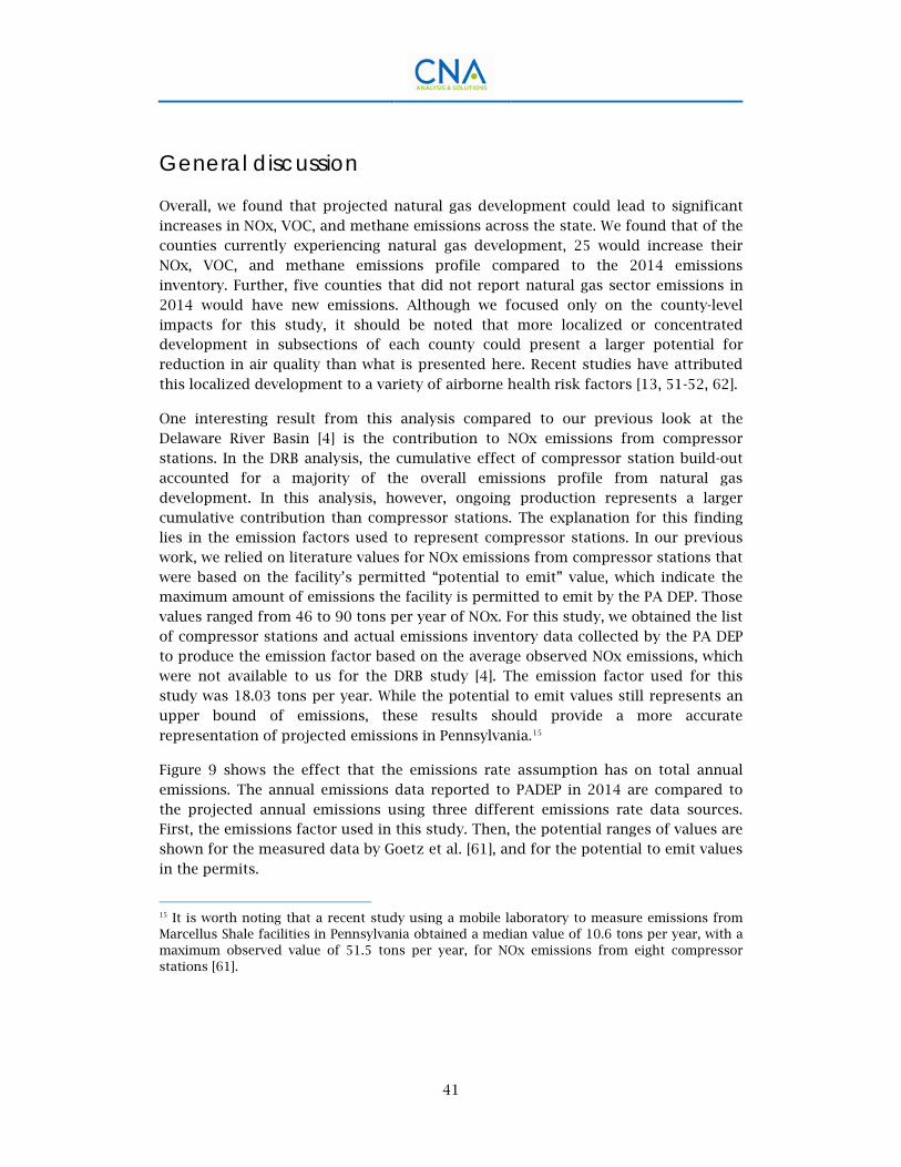
41

General discussion

Overall, we found that projected natural gas development could lead to significant increases in NOx, VOC, and methane emissions across the state. We found that of the counties currently experiencing natural gas development, 25 would increase their NOx, VOC, and methane emissions profile compared to the 2014 emissions inventory. Further, five counties that did not report natural gas sector emissions in 2014 would have new emissions. Although we focused only on the county-level impacts for this study, it should be noted that more localized or concentrated development in subsections of each county could present a larger potential for reduction in air quality than what is presented here. Recent studies have attributed

this localized development to a variety of airborne health risk factors [13, 51-52, 62].

One interesting result from this analysis compared to our previous look at the Delaware River Basin [4] is the contribution to NOx emissions from compressor stations. In the DRB analysis, the cumulative effect of compressor station build-out accounted for a majority of the overall emissions profile from natural gas development. In this analysis, however, ongoing production represents a larger cumulative contribution than compressor stations. The explanation for this finding lies in the emission factors used to represent compressor stations. In our previous work, we relied on literature values for NOx emissions from compressor stations that were based on the facility’s permitted “potential to emit” value, which indicate the maximum amount of emissions the facility is permitted to emit by the PA DEP. Those values ranged from 46 to 90 tons per year of NOx. For this study, we obtained the list of compressor stations and actual emissions inventory data collected by the PA DEP to produce the emission factor based on the average observed NOx emissions, which were not available to us for the DRB study [4]. The emission factor used for this study was 18.03 tons per year. While the potential to emit values still represents an upper bound of emissions, these results should provide a more accurate

representation of projected emissions in Pennsylvania.15

Figure 9 shows the effect that the emissions rate assumption has on total annual emissions. The annual emissions data reported to PADEP in 2014 are compared to the projected annual emissions using three different emissions rate data sources. First, the emissions factor used in this study. Then, the potential ranges of values are shown for the measured data by Goetz et al. [61], and for the potential to emit values

in the permits.

15 It is worth noting that a recent study using a mobile laboratory to measure emissions from Marcellus Shale facilities in Pennsylvania obtained a median value of 10.6 tons per year, with a maximum observed value of 51.5 tons per year, for NOx emissions from eight compressor stations [61].

42

Figure 9. Uncertainty in statewide Marcellus annual NOx emissions due to emissions factor used for natural gas gathering compressor stations. Annual emissions reported to PADEP for 2014 are shown for comparison. (Emissions attributed to pre-production and production are the same for all cases at 29,300 tons.)

Source: CNA, based on data from: PA DEP [59], Goetz et al., 2015 [61]

Given that NOx and VOC are the precursors to ozone formation, a potential by-product of increased development is an increase in ozone formation for the impacted counties. A recent study found that natural gas development in the Barnett Shale contributed to an increase in ozone pollution in the Dallas-Fort Worth area [63]. Ground-level ozone is a primary component of smog, which can cause respiratory illness and other decreases in lung function. Due to its potential to cause harm to human health, the EPA monitors ozone, and this pollutant is subject to national ambient air-quality standards (NAAQS). The Pittsburgh-Beaver Valley region (i.e., Allegheny County and the surrounding counties) has struggled in the past with air quality issues related to ozone and even received a non-attainment status for ozone [64]. Projected development in this area could further contribute to these air quality

issues.

Some potential follow-on analysis possibilities include scenario or contextual analysis. For example, a study could investigate effects of timing or rate of development in order to refine and evaluate the air quality impacts in each county over time. Or, a different study could compare the projected air quality impacts from gas development to air quality impacts from other sectors in order to

determine the impact on total emissions in each county and state-wide.

(18.03)

Min (1.8)

Low (46)

Max (51.5)

High (90)

Median (10.6)

010,00020,00030,00040,00050,00060,00070,00080,000

PADEP 2014 This study Measured[61]

Pot. to Emit(permit)

Stat

ewid

e N

Ox

emiss

ions

(t

ons/

yr) (Assumed per

well NOx emissions factor for compressor stations shown in parentheses.)

43

Water and Wastewater Impact

Water and wastewater management is a significant part of the unconventional natural gas extraction process. Hydraulic fracturing requires a significant amount of water to mix the “frac fluid” that is pumped into the horizontal wells at high pressure in order to fracture the shale and release gas. Most of the water needed to mix the frac fluid is withdrawn from nearby surface water resources, though some of the water needs are met through recycling of wastewater, groundwater, and other

sources (e.g., purchase from municipal water providers).

After injection, most of the frac fluid remains in the shale formation, but some returns to the surface along with the gas. The early portion of the water that returns in the first 10–30 days is known as flowback. Later, additional wastewater known as “produced water” or “brine” returns with the gas for as long as the gas well is producing, and roughly in proportion with gas production. Both flowback and produced water are types of wastewater with high concentrations of dissolved solids (salts), metals, volatile organic compounds, and, in some cases, radioactive materials. Some of these contaminants may originate as additives in frac fluid, but many are picked up from the shale formation itself. The final type of wastewater is drilling fluid recovered after drilling the wells. (There are also several types of solid waste, including drill cuttings, and solids settled out from flowback or produced water, but

they are not part of this analysis.)

In this analysis, we analyze the volumes of water and wastewater associated with the projected development of gas wells in the Interior Marcellus. Notably, we focus on

four key metrics related to natural gas water management:

• Water use: the total volume of water used for mixing the frac fluid that is

injected into the shale during hydraulic fracturing

• Water withdrawal: the volume of water used to mix frac fluid that is

withdrawn from surface water resources

• Consumptive use: the volume of water in the frac fluid that remains in the

shale after injection

• Wastewater generation: the volume of wastewater produced from the wells as

either flowback or produced water plus used drilling fluid.

44

All of these metrics are important as they can be used for different impact assessments. Water use is important to report, as it is the total volume of water needed for hydraulic fracturing regardless of source. In theory, all of this water could be taken from local streams, but in many cases, other water sources are used including groundwater and recycled wastewater (either from the natural gas industry or from municipal or industrial wastewater sources). For this reason, water withdrawal is reported as the average quantity that would be taken from local streams. After frac fluid injection, some portion of the water used for fracking comes back as wastewater, and can potentially return to the watershed (after some level of wastewater treatment). But the consumptive use - or the portion of frac fluid does not return - is important to understand as it indicates the (minimum) amount flow is reduced in the watershed. Finally, it is important to understand the volume of wastewater generated that must be managed due to the potential risks associated

with the high concentrations of water pollutants it natural gas wastewaters[4].

All of these metrics refer to water volumes, but considering the large number of wells involved, and the long period of well development, reporting volumes for these metrics would result in very large numbers that are difficult to put into context. Instead, we report these metrics in terms of average flow rate—that is, volume per unit of time. We assume a 30-year development period as the unit of time, so all of the metrics are expressed as the average volume over that period. We use the U.S. Geological Survey’s preferred unit of flow, cubic feet per second (cfs) to report these metrics in the results. We also report the 30-year statewide total volume in billions of

gallons. (1 cubic foot equals 7.48 gallons.)


In this report, we use four major metrics for water use for fracking. They relate to the major water management stages for unconventional gas development with hydraulic fracturing.

For calculation of water and wastewater impacts, we assume that:

• Well development will occur at eight wells per well pad on average. Each well

is fracked once, and there is no-re-stimulation.16

• All wells within a HUC-8 have the same water use.

16 Some wells can be re-stimulated (or-refracked) to boost or prolong gas recovery. There has been limited re-fracking to date, and few data exist on the amount of water needed. We have not included re-fracking in this analysis.

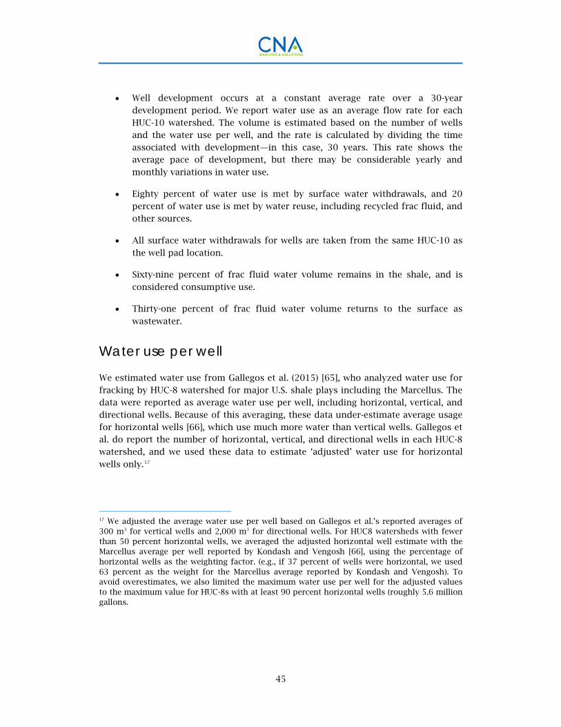
45

• Well development occurs at a constant average rate over a 30-year development period. We report water use as an average flow rate for each HUC-10 watershed. The volume is estimated based on the number of wells and the water use per well, and the rate is calculated by dividing the time associated with development—in this case, 30 years. This rate shows the average pace of development, but there may be considerable yearly and

monthly variations in water use.

• Eighty percent of water use is met by surface water withdrawals, and 20 percent of water use is met by water reuse, including recycled frac fluid, and other sources.

• All surface water withdrawals for wells are taken from the same HUC-10 as

the well pad location.

• Sixty-nine percent of frac fluid water volume remains in the shale, and is

considered consumptive use.

• Thirty-one percent of frac fluid water volume returns to the surface as

wastewater.

Water use per well

We estimated water use from Gallegos et al. (2015) [65], who analyzed water use for fracking by HUC-8 watershed for major U.S. shale plays including the Marcellus. The data were reported as average water use per well, including horizontal, vertical, and directional wells. Because of this averaging, these data under-estimate average usage for horizontal wells [66], which use much more water than vertical wells. Gallegos et al. do report the number of horizontal, vertical, and directional wells in each HUC-8 watershed, and we used these data to estimate ‘adjusted’ water use for horizontal

wells only.17

17 We adjusted the average water use per well based on Gallegos et al.’s reported averages of 300 m3 for vertical wells and 2,000 m3 for directional wells. For HUC8 watersheds with fewer than 50 percent horizontal wells, we averaged the adjusted horizontal well estimate with the Marcellus average per well reported by Kondash and Vengosh [66], using the percentage of horizontal wells as the weighting factor. (e.g., if 37 percent of wells were horizontal, we used 63 percent as the weight for the Marcellus average reported by Kondash and Vengosh). To avoid overestimates, we also limited the maximum water use per well for the adjusted values to the maximum value for HUC-8s with at least 90 percent horizontal wells (roughly 5.6 million gallons.

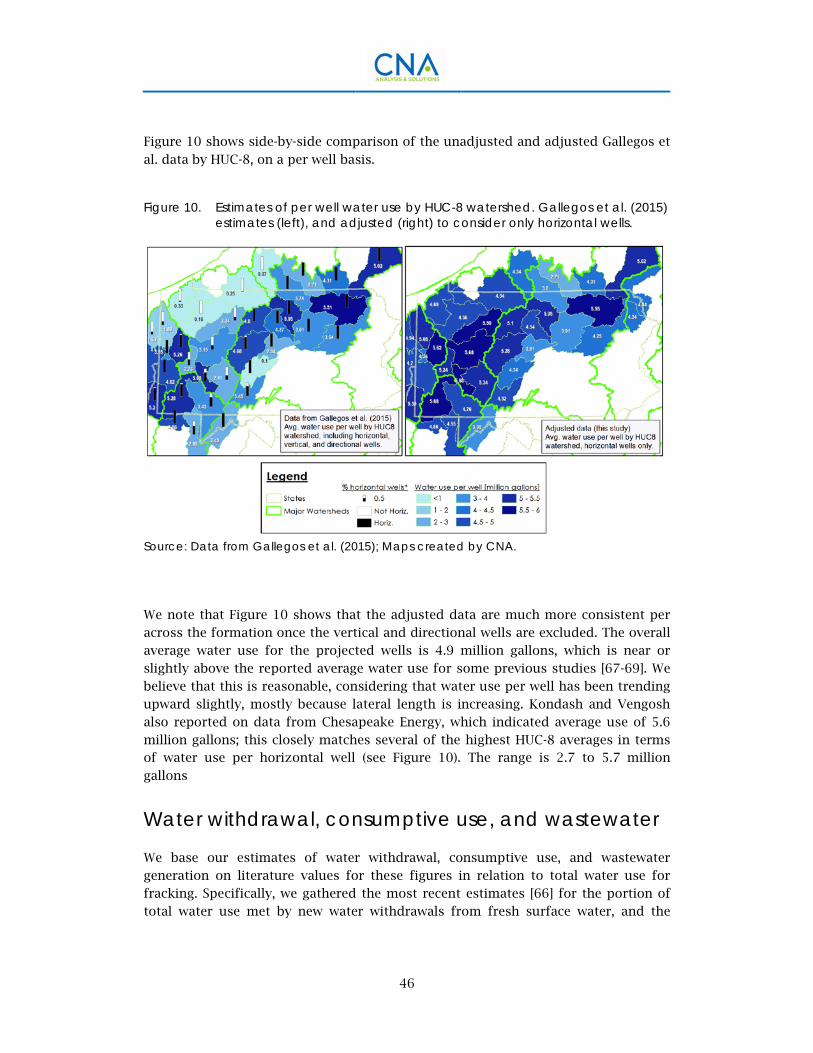
46

Figure 10 shows side-by-side comparison of the unadjusted and adjusted Gallegos et

al. data by HUC-8, on a per well basis.

Figure 10. Estimates of per well water use by HUC-8 watershed. Gallegos et al. (2015) estimates (left), and adjusted (right) to consider only horizontal wells.

Source: Data from Gallegos et al. (2015); Maps created by CNA.

We note that Figure 10 shows that the adjusted data are much more consistent per across the formation once the vertical and directional wells are excluded. The overall average water use for the projected wells is 4.9 million gallons, which is near or slightly above the reported average water use for some previous studies [67-69]. We believe that this is reasonable, considering that water use per well has been trending upward slightly, mostly because lateral length is increasing. Kondash and Vengosh also reported on data from Chesapeake Energy, which indicated average use of 5.6 million gallons; this closely matches several of the highest HUC-8 averages in terms of water use per horizontal well (see Figure 10). The range is 2.7 to 5.7 million

gallons

Water withdrawal, consumptive use, and wastewater

We base our estimates of water withdrawal, consumptive use, and wastewater generation on literature values for these figures in relation to total water use for fracking. Specifically, we gathered the most recent estimates [66] for the portion of total water use met by new water withdrawals from fresh surface water, and the

47

relative proportion of injected frac fluid that remains in the shale (consumptive use)

versus returns as flowback or brine wastewater.

We assume that most of the water demand for hydraulic fracturing will be met by surface water withdrawals. Trends in the industry are towards more reuse of natural gas wastewaters for water supply, and there has been some interest in non-traditional sources such as municipal wastewater treatment plant effluent or mine drainage waters. For this study, consistent with the previous CNA study for the Delaware River Basin, we assume that 80 percent of the total water use for fracking is met by surface water withdrawals, which accounts account for wider availability of recycled wastewater as more wells are developed. This percentage is slightly below figures by other research on the topic [68-69], though comparable to recent data published by the Susquehanna River Basin Commission [70]. Transporting water is a significant cost, so we assume that all wells will be supplied by surface water withdrawals from within the same watershed (i.e., HUC-10) as the well pad site. At this level of analysis, we make no assumption about the stream order within the watershed from which the withdrawal is taken. Finally, we assume that the 80

percent factor is constant across the study area.

For determining the fate of the injected water in the frac fluid, we used recent research by Kondash and Vengosh (2015) [66]. Early analysis of unconventional drilling in the Marcellus Shale had indicated that only a small portion, perhaps 10-15 percent, of water injected as frac fluid would return to the surface as natural gas wastewater. But these analyses were mostly focused on the flowback fluid, which can be measured easily as it returns over the first 30 days after hydraulic fracturing. Kondash and Vengosh, by contrast, accounted for more of the produced water which comes up the well in small quantities along with produced gas for 10 years or longer. Taking this longer view, Kondash and Vengosh calculated that 31 percent of the average injected frac fluid volume would return as wastewater. The remaining 69 percent is “consumptive use” as it is not recovered from the shale. Since our study covers a long time horizon, we use these figures to calculate consumptive use and volume of wastewater generated. We assume that these percentages remain constant

across the study area.18

18 We did investigate Pennsylvania Oil and Gas wastewater reporting data for geographic trends in wastewater volume, but we found insufficient data to clearly indicate geographic differences. In many cases, we could not connect water use per well from FracFocus with wastewater records. Additionally, the wastewater reporting data were often incomplete due to omissions or, more likely, because not enough time had passed since drilling and fracking to collect, process, and report wastewater volumes.

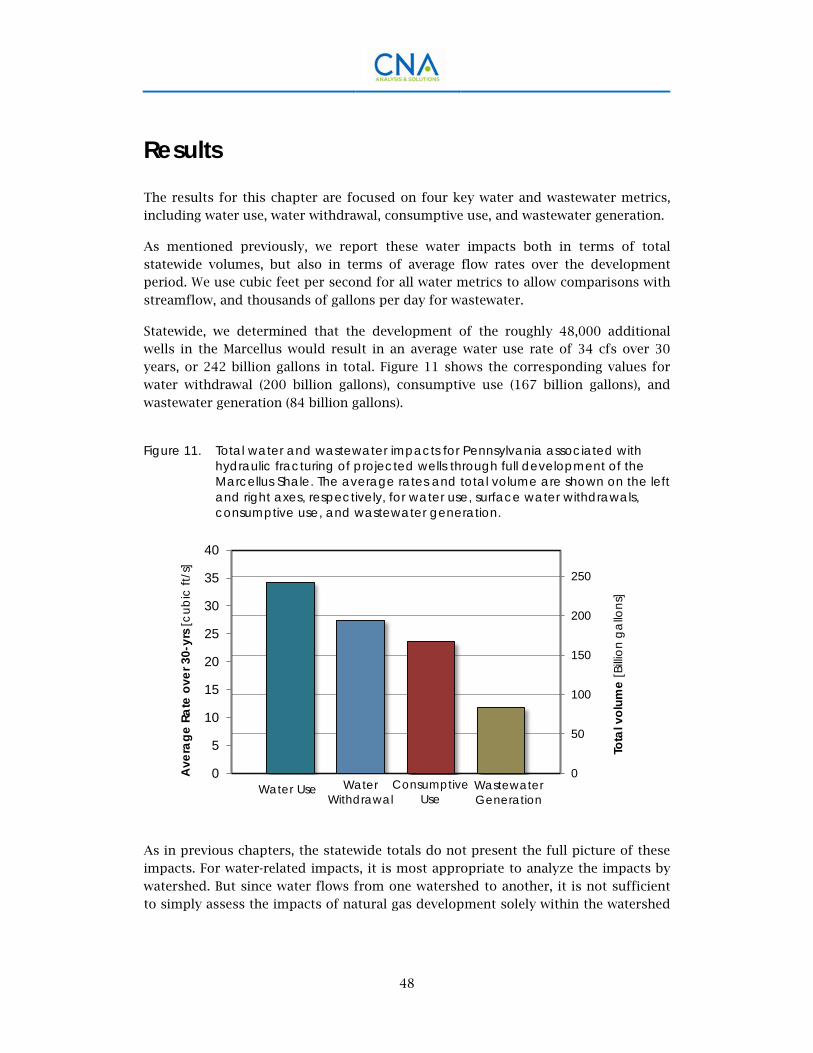
48

Results

The results for this chapter are focused on four key water and wastewater metrics, including water use, water withdrawal, consumptive use, and wastewater generation.

As mentioned previously, we report these water impacts both in terms of total statewide volumes, but also in terms of average flow rates over the development period. We use cubic feet per second for all water metrics to allow comparisons with

streamflow, and thousands of gallons per day for wastewater.

Statewide, we determined that the development of the roughly 48,000 additional wells in the Marcellus would result in an average water use rate of 34 cfs over 30 years, or 242 billion gallons in total. Figure 11 shows the corresponding values for water withdrawal (200 billion gallons), consumptive use (167 billion gallons), and

wastewater generation (84 billion gallons).

Figure 11. Total water and wastewater impacts for Pennsylvania associated with hydraulic fracturing of projected wells through full development of the Marcellus Shale. The average rates and total volume are shown on the left and right axes, respectively, for water use, surface water withdrawals, consumptive use, and wastewater generation.

As in previous chapters, the statewide totals do not present the full picture of these impacts. For water-related impacts, it is most appropriate to analyze the impacts by watershed. But since water flows from one watershed to another, it is not sufficient to simply assess the impacts of natural gas development solely within the watershed

Water Use Water Withdrawal

Consumptive Use

Wastewater Generation

0

50

100

150

200

250

0

5

10

15

20

25

30

35

40

Tota

l vol

ume

[Billi

on g

allo

ns]

Ave

rage

Rat

e ov

er 3

0-yr

s [cu

bic

ft/s]

49

the development occurs. We have generated four categories of maps to give greater

understanding and context to this analysis.

• Volume/Flow-rate – Standard analysis of water-related impacts in each HUC-10 watershed based only on development within the watershed, expressed as

average-flow over the development period.

• Specific or Area-averaged flow – measures the ‘intensity’ of water use by dividing the flow computed for each watershed by watershed area. This will

show where development will be most concentrated.

• Cumulative flow – presents a more comprehensive view of the water impacts by including both the impacts within each watershed and the total impact from

all watersheds upstream. This is particularly relevant to consumptive use.

• Contextual analysis – compares the flow-rates calculated in this analysis to

existing water usage.

Table 7 presents an overview of the water and wastewater maps by metric and category. Not all categories of map are relevant for all of the metrics. Maps 5.1–5.4 present the water use, withdrawal, consumptive use, and wastewater generation by HUC-10 watershed in terms of average flow rate. Maps 5.5 and 5.6 present area-averaged or “specific” flow rates for water use and water withdrawal. Since assessing the water use in each watershed individually does not present the full picture of how water flows between watersheds, we created Maps 5.7 and 5.8 to show cumulative water use and consumptive use for each watershed including the upstream usage. Finally, in Map 5.9, we compare consumptive use for hydraulic fracturing relative to

all other consumptive uses, this time at the larger HUC-8 watershed scale.

Table 7. Water and wastewater maps by metric and category.

Metric Volume/ Flow-rate

Area-averaged flow

Cumulative flow

Contextual analysis

Water Use Map 5.1 Map 5.5 Map 5.7 Water Withdrawal Map 5.2 Map 5.6 Consumptive Use Map 5.3 Map 5.8 Map 5.9

Wastewater Generated Map 5.4

50

Table 8 introduces the maps generated for this category. The following discussion

section offers commentary on how to read and interpret each map.

Table 8. Water and Wastewater Impacts Map Index. Access maps at www.cna.org/PA-Marcellus

Map Title 5.1 Water use by watershed 5.2 Water withdrawal by watershed 5.3 Consumptive water use by watershed 5.4 Wastewater generation by watershed 5.5 Specific water use 5.6 Specific water withdrawal 5.7 Cumulative water use 5.8 Cumulative consumptive use 5.9 Consumptive use relative to existing consumptive uses

Discussion

Map 5.1 – Water use by watershed

This map shows projected water use for hydraulic fracturing by HUC-10 watershed. The water use metric represents total water use volume for hydraulic fracturing by all projected wells within each HUC-10 through build-out, expressed as flow rate in cubic feet per second (cfs). The rate represents the average water use rate over the full build-out time frame, assumed to be 30 years. This metric does not include water

uses for anything other than fracking (e.g., for drilling fluid or site preparation).

To generate this map, we used well projection numbers on a HUC-10 basis and the adjusted estimates of water use per well, which are computed from Gallegos et al. [65] on a HUC-8 basis. Therefore, the differences in the results by HUC-10 reflect differences in projected number of wells developed, and geographic differences in

the average amount of water used for hydraulic fracturing.

Map 5.2 – Water withdrawal by watershed

This map shows the projected freshwater withdrawal for hydraulic fracturing through build-out by HUC-10 watershed. This metric represents total freshwater withdrawal volume for hydraulic fracturing by all projected wells within each HUC-10 through build-out, expressed as flow rate in cubic feet per second. The freshwater withdrawal rate is less than total water use rate because we assume that 20 percent


51

of the total water use for hydraulic fracturing is met by other water sources,

primarily wastewater reuse, instead of freshwater withdrawal.

Map 5.3 – Consumptive use by watershed

This map shows the projected consumptive use associated with hydraulic fracturing through build-out by HUC-10 watershed. This metric represents the volume of hydraulic fracturing fluid left within the shale for all projected wells within each HUC-10 through build-out, expressed as flow rate in cubic feet per second. The consumptive water use rate is less than total water use rate because a portion of the injected fluid returns to the surface as wastewater.

We assume a standard fixed relationship across the Marcellus for percentage of the total water used for hydraulic fracturing that is left in the shale as consumptive use. Based on figures from Kondash and Vengosh [66], we assume that consumptive use

is, on average, 69 percent of total water use for hydraulic fracturing.

Map 5.4 – Wastewater generation by watershed

This map shows the projected wastewater generation associated with hydraulic fracturing through build-out by HUC-10 watershed. This metric represents the volume of natural gas wastewaters returning from the shale after fracking for all projected wells plus drilling fluid wastewater within each HUC-10 through build-out, expressed in thousands of gallons per day. The wastewater generation rate for flowback and produced water is equal to total water use rate minus the consumptive use rate (water from the injected fluid left in the shale), or simply 31 percent of the total water use rate. We added another 185,000 gallons per well for drilling wastewater, slightly higher than the amount in previous research [71] to account for increasing lateral length.

This metric indicates the total volume of wastewater that must be handled within each HUC-10 watershed. This analysis does not consider how the wastewater is managed, treated, recycled, transported, or discharged. Separate analyses would be needed to determine how different wastewater treatment or disposal methods may affect water quality, human health, or ecological outcomes. The map does show currently (as of April 2016) permitted facilities for handling oil and gas wastewaters,

for context.

Map 5.5 – Specific water use

This map, similar to Map 5.1, shows water use for hydraulic fracturing by HUC-10 watershed. The water use metric is identical to the one in Map 5.1, but is normalized

52

to the area of the watershed. The metric is presented as water withdrawal in cubic feet per second per 100 square miles. We use 100 square miles to make the numbers easier to comprehend, and because HUC-10 watersheds are on the order of 100 square miles in area. We could also present this metric as a depth over the watershed. For conversion, 1 cfs per 100 square miles (for a year) is equivalent to a depth on the watershed of 0.136 inches, or 3.45 millimeters, per year.

In Map 5.1, the largest watersheds typically also show the highest water use because they contain more well pads due to their size. Normalizing by watershed area removes this issue, and Map 5.5 shows the watersheds with high water use because

they have a high relative density of development.

Map 5.6 – Specific water withdrawal

This map, similar to Map 5.2, shows freshwater withdrawal associated with hydraulic fracturing by HUC-10 watershed. The water withdrawal metric is identical to the one in Map 5.2, but is normalized to the area of the watershed. The metric is presented as

water withdrawal in cubic feet per second per 100 square miles.

In Map 5.2, the largest watersheds typically also show the highest water withdrawal because they contain more well pads due to their size. Normalizing by watershed area removes this issue, and Map 5.6 shows the watersheds with high water

withdrawal because they have a high relative density of development.

(Note: We do not show similar maps for consumptive use or wastewater generation because the relationship between the direct flow rate map and area-averaged map is

similar to those for water use and water withdrawal.)

Map 5.7 – Cumulative water use

This map shows cumulative projected water use for hydraulic fracturing by HUC-10 watershed. The water use metric represents total water use volume for hydraulic fracturing by all projected wells within each HUC-10 through build-out plus the water use for all upstream HUC-10s, expressed as flow rate in cubic feet per second (cfs). This metric shows the cumulative upstream water use on an average basis through

build-out.

This map is similar to Map 5.1, but adds all of the upstream water use to the water use for each HUC-10. This map shows water use in more HUC-10 watersheds than Map 5.1 because the water use is traced farther downstream until all water use for hydraulic fracturing is captured. In some cases, the watersheds are outside of Pennsylvania. This metric does show total upstream water use for hydraulic fracturing on an average basis, but the metric may not be meaningful with respect to

53

streamflow because alternate water sources and return flow (after wastewater treatment) are not taken into account. A more physically meaningful cumulative

water use metric is the consumptive use, which is shown in Map 5.8.

The map also labels the average daily water use by major river basin. (Note that the Upper Ohio includes the cumulative flow from both the Allegheny and Monongahela.) Based on current data, these estimates appear reasonable; the Susquehanna River Basin Commission reported total water use of 15.4 cfs for 2012, and 13.2 cfs for

2013 [70], closely matching the 13.9 cfs reported for this study.

Map 5.8 – Cumulative consumptive use

This map shows cumulative projected consumptive use associated with hydraulic fracturing by HUC-10 watershed. This metric represents total consumptive water use volume associated with hydraulic fracturing by all projected wells within each HUC-10 through build-out plus the consumptive use for all upstream HUC-10s, expressed

as an average flow rate in cfs.

This map is similar to Map 5.3, but adds all of the upstream consumptive use to the consumptive use for each HUC-10. It shows, on an average basis, the potential reduction in streamflow at the outlet point of each HUC-10 watershed. This map shows consumptive use in more HUC-10 watersheds than Map 5.3 because the water use is traced farther downstream until all water use for hydraulic fracturing in the Marcellus formation in Pennsylvania is captured. In some cases, the watersheds are outside of Pennsylvania due to the flow of rivers across state boundaries. Actual consumptive use could be higher or lower depending on how water is sourced and how wastewater is handled (recycling versus treatment with effluent disposal versus deep well injection). The consumptive use will also vary considerably over time and

space due to variations in development rate.

For context, the total cumulative consumptive use for gas development at Pittsburgh is roughly 10.9 cfs (Allegheny plus Monogahela). Pittsburgh’s municipal water supplier, PWSA, treats roughly 70 million gallons per day, or 108 cfs of potable water supply. Assuming a typical consumptive use rate of 10 percent for municipal supply, Pittsburgh’s consumptive use for water supply is roughly 10.8 cfs (i.e., almost exactly equal to the average consumptive use for hydraulic fracturing upstream of Pittsburgh). Map 5.9 shows similar comparisons statewide, but for all existing

consumptive water uses including agricultural and industrial use.

(Note: We did not generate similar maps to Maps 5.7 and 5.8 for water withdrawal or wastewater generation. The water withdrawal map would be similar to Map 5.7, and would not account for possible return flow after wastewater treatment. A cumulative wastewater generation map would not be especially instructive unless we assumed

54

that all wastewater is returned to the same watershed in which it was produced, and

is not reused or transported to other watersheds for treatment.)

Map 5.9 – Consumptive use by watershed relative to existing consumptive uses

This map shows projected consumptive use for hydraulic fracturing on a HUC-8 basis, and relative to all other existing consumptive uses. We acquired the baseline consumptive use data by HUC-8 from Caldwell et al. (2013) [72], which is based on 2005 USGS water use data disaggregated to HUC-8 scale, and accounts for end use specific and geographically specific consumptive use factors relative to reported water use. These data would predate water usage related to UNGD with HVHF, but

also do not account for changes in water use over the past decade.

The map shading indicates the total volume of consumptive water use associated with hydraulic fracturing by all projected wells within each HUC-8 through build-out, expressed as an average rate over 30 years. Using the vertical bars, we indicate the ratio of this consumptive use associated with fracking over the total estimated consumptive use for each HUC-8 as a percentage. This metric can be read as either the ratio of UNGD consumptive use to existing (2005) consumptive use, or the amount by which consumptive use would increase over existing usage in the HUC-8

due to UNGD.

This map puts the consumptive use for hydraulic fracturing in context with existing consumptive uses. In some areas of Pennsylvania, water use for fracking could dramatically increase overall consumptive use. In other areas (even with similar average usage for fracking), the existing consumptive use is much higher and the

ratio is lower.

General discussion

The analysis presented considers four primary volumetric water and wastewater metrics presented on an average basis over a 30-year development period. This analysis considers only the total volumes of water and wastewater associated with hydraulic fracturing, presented as an average rate over a 30-year development horizon.

For at least four reasons, this analysis does not capture the full potential impacts of water and waste management associated with natural gas development. First, there are additional water uses and wastes that are not included in this analysis. Some additional water use is associated with indirect uses such as site preparation, materials processing and quarrying, and equipment washing. [68] Other waste

55

streams including spent lubricants and solid wastes such as drilling cuttings are not

considered in this report. [16]

Secondly, the well development rate, and by extension the water use rate will vary geographically and temporally. The pace of development will likely correlate with energy prices, ability to sign leases, ability to permit and construct natural gas infrastructure, and other factors. The pace of development in turn affects flow rates associated with all phases of water management. The freshwater withdrawal rate could be several times higher than the average rate during peak periods [4], which can increase potential impacts on streams. Likewise, the consumption rate and

wastewater generation rate will increase.

Thirdly, there may be variability in the water use rates from well to well19, and there may be changes over time due to evolving industry practices and regional development characteristics. Recently, water use per well has been increasing as average lateral length and the number of fractures per well has increased [70] (though primarily in “hotspot” areas with especially rich gas deposits). In addition, seasonal variations in drilling and hydraulic fracturing activity may play a large role in timing of withdrawals. Also, as development continues, more wastewater will be available for reuse, which could lower the portion of water use met by freshwater withdrawal for wells developed later. Finally, re-fracking is not included in this analysis, but could raise water usage in some areas of the play. Capturing these temporal aspects of water management is beyond the scope of this study, and would require a methodology for projecting well development on a year-by-year (or even

month-by-month) basis.

Fourth, there is potential for movement of water and wastewater across watersheds. We assume that the demand for water withdrawal is met within the same HUC-10 as the well pad. This is generally a reasonable assumption, but in some cases may not be correct. Given costs to permit and develop new water withdrawals, it is possible that an existing, permitted water withdrawal location in an adjacent HUC-10 may make more sense for a particular well pad or operator. Our analysis focuses only on wastewater generation by watershed, as significant quantities of natural gas wastewaters (and other wastes) are routinely transported even across major river basin boundaries [16], and a full examination of wastewater disposal scenarios was

beyond the scope of this study.

19 The data we used had a range of per well water use (averaged over each HUC-8) from 2.7 to 5.7 million gallons per well, an average of 4.9, and a median of 5.0. The total water use we computed for the projected 47,600 wells is 242 billion gallons based on the average computed for each HUC-8. If all wells used water at the highest end of the range, the total water use would be 270 billion gallons, an 11 percent increase.

56

Overall, this analysis generates projections of water and wastewater volumes, but does not investigate the context of the source (or receiving waters). That is, this is an analysis of environmental “burdens”, but not “impacts”. We present the water volumes in terms of flow rates, which is useful for supporting additional research. Specifically, this analysis does not put the magnitude of withdrawals and wastewater volumes into context by comparing them to the available streamflow in the watershed. Just as there can be significant variations in the rates of water use and wastewater generation, the actual impacts of water withdrawals on stream flow are highly dependent on the location of withdrawal, and the natural variability in the flow of the source waters. Withdrawing water in the spring from the mainstem of the Susquehanna River may have a negligible impact on flow, while withdrawing from a

small headwater stream during late summer could have a substantial impact.

Similarly, we report only the wastewater volumes associated with development, and do not investigate potential impacts on water quality. Disposal of treated natural gas wastewaters can raise the concentration of certain pollutants (e.g., dissolved solids, barium, strontium, bromide) with potential ecological and human health effects. Our previous report on the Delaware River basin [4] investigated the potential impacts of water usage on available flow, and disposal of treated wastewater on the in-stream concentrations of pollutants for three case study watersheds, and found that the level of impact did vary (often by an order of magnitude) with development rate, in-

stream flow, and stream order.

There are several ways this analysis could support additional studies. Examining the effects of water withdrawals on available flow is a logical extension. The wastewater impacts, however, may be of particular concern, especially given the potential risks to drinking water supplies. [5, 73-78] The method of wastewater management (e.g., on-site reuse of wastewater, treatment at a centralized wastewater facility, or exporting wastewater for disposal via deep well injection) is important; each has very different consequences for water quality. Investigating potential water quality impacts and key vulnerabilities (ecosystem and human health) for various wastewater management scenarios could be a useful topic for future analysis, and

informing policy.

57

Conclusion

Unconventional natural gas development using hydraulic fracturing has spurred a rapid expansion of natural gas extraction in Pennsylvania due to the presence of the Marcellus Shale—which, though rich in gas, could not be economically developed with traditional drilling methods. Through the almost nine years of unconventional gas development in Pennsylvania, the Commonwealth has witnessed significant changes to energy costs, employment, communities, and the environment. While the price of natural gas has led to fluctuations in the amount of development, the quantity of remaining gas reserves in the Marcellus Shale could support significantly

more gas development in coming years.

In this study, we ask, “What would be the environmental burdens associated with natural gas development activities in Pennsylvania if the Interior Marcellus Shale

resources were fully developed?”

Specifically, we investigate the potential impacts to Pennsylvania’s land, forests, water, air, and population if development of the Marcellus Shale were to continue

until all of the technically recoverable reserves were exhausted.

One significant difficulty with investigating potential future impacts of gas development is determining where those impacts may occur. To address this challenge, we developed a geospatial analysis methodology to identify the most likely locations of potential future wells, based on finding geologic, environmental, and land use conditions similar to where wells have already been drilled. Using the probability surface generated from this analysis and recent estimates of total recoverable reserves and average production per well, we determined how many wells would be developed until reserves are depleted, and their most likely locations. That is, we developed one set of “projections” of well numbers and locations through (what is currently estimated) as build-out condition. These are not formal predictions of wells and their locations, just one possible configuration identified as likely based

on current information on gas development in the Interior Marcellus Shale.

With information on well locations and level of impact per well, we analyze the spatial characteristics of impacts of natural gas development. For the most part, we compute these impacts based on the well (or well pad) numbers in a given geographic unit, and impacts per well or well pad derived from published literature or data sets. We also apply additional geospatial and mathematical analysis techniques to

estimate several of the impacts, as appropriate.

58

The primary output of this research is an atlas: a set of maps that puts the impacts of the projected natural gas development in useful spatial context. These maps, and the data developed to generate them, present useful information to policy-makers, decision-makers, and other researchers concerned about managing the range of impacts of shale gas extraction in Pennsylvania. We strive to present the impacts using straightforward, relevant metrics useful for comprehension and supportive of follow-on analysis. At this time, the metrics are focused on environmental burdens and impacts (e.g., land areas, emissions, volumes, and flow rates) that can be reasonably and directly estimated from the well and well pad projections. This analysis does not address the potential “outcomes” resulting from the impacts (e.g., endangered species populations, water pollutant concentrations, and human health

outcomes).

Key findings

For the Commonwealth of Pennsylvania, the key impacts we determined to be associated with the full development of the Marcellus Interior shale formation

include:

• Well development – We estimated that 47,600 additional wells could be developed on 5,950 well pads over the next 30 years if the Interior

Marcellus’s technically recoverable resources were fully developed.

• Land use change – The construction of natural gas infrastructure (well pads,

gathering pipelines, and access roads) to support projected well development would result in almost 100,000 acres of land disturbance. Over half (about 51,000 acres) of the land disturbance would impact agricultural land, while

about 28,000 acres would constitute the clearing of forest cover.

• Forest change – Of the 28,000 acres of forest that would be cleared, we

found that nearly 13,000 acres were core forest (patches of forest at least 300 feet from a forest edge). An additional 89,000 acres of core forest would be fragmented by the projected gas infrastructure development, resulting in

a conversion to edge forest.

• Population in proximity to well pads – We estimated that the current population in Pennsylvania living within one-half mile of a well pad is about 100,000, and this number could increase to 639,000 based on our projections. Similarly, we estimate that the population living within one mile of a well pad could increase from about 311,000 today to over 1.8 million at

full build-out.

59

• Air emissions – The additional well development would result in greater emissions of NOx, VOCs, and CH

4 from activities related to well pre-

production, and production, and compressor stations for moving gas through gathering lines. When the play nears full development (i.e., ongoing emissions from producing wells reach their peak), the average air emissions per year could reach 37,000 tons for NOx, 22,500 tons for VOCs, and 342,000 tons for

methane.

• Water use, withdrawal, and consumptive use – We determined that the projected natural gas development in the Marcellus would result in an average water use rate of 34 cfs over about 30 years, or 242 billion gallons in total in order to mix frac fluid for the hydraulic fracturing process. We found that roughly 200 billion gallons of fresh surface water would be withdrawn to support this development, and that 167 billion gallons would be used

consumptively and would not re-join the hydrologic cycle after injection.

• Wastewater generated – We estimated that 84 billion gallons of wastewater would be generated from projected natural gas development in Pennsylvania. Wastewater includes drilling fluid waste, plus flowback and produced water/brine recovered from the shale after frac fluid injection and during gas

production.

All of these metrics offer a sense of the scale of the total statewide impacts of natural gas development through full development of the Marcellus Shale. But these aggregated metrics do not tell the full story of the impacts, which have important geographic variations. The maps accompanying this work show these variations and can help identify areas of comparatively higher and lower impacts. Readers are

encouraged to view and download these maps at: www.cna.org/PA-Marcellus

We do not provide an opinion on the overall significance of these impacts—we leave that to policy-makers and decision-makers with local knowledge of the impacted areas to decide. But this analysis takes the initial step of looking at the long-term future of natural gas development in Pennsylvania. Development appears likely to continue over the coming years, and will continue to have some level of environmental impact wherever development occurs. Tolerance for and management of these impacts will be a continuing area of debate among policy-makers, regulators, land owners, the natural gas industry, and the general public. This analysis provides information that any of the relevant stakeholders—especially policy-makers—may consider as they decide how gas development is to be managed and regulated over

the coming decades.


60

References

[1] Hanson, Mark P. 2014. “Shale Shock - How the Marcellus Shale Transformed the Domestic Natural Gas Landscape and What It Means for Supply in the Years Ahead.” Morningstar Energy Observer. February 2014.

[2] Hughes, J. David. 2014. Drilling Deeper - A reality check on U.S. government forecasts for a lasting tight oil & shale gas boom. Post Carbon Institute. http://www.postcarbon.org/publications/drillingdeeper/.

[3] Staub, John. 2015. “The Growth of U.S. Natural Gas: An Uncertain Outlook for U.S. and World Supply.” 2015 EIA Energy Conference, Washington, DC, June 15, 2015. http://www.eia.gov/conference/2015/pdf/presentations/staub.pdf.

[4] Habicht, S., L. Hanson, and P. Faeth. 2015. The Potential Environmental Impact from Fracking in the Delaware River Basin. https://www.cna.org/cna_files/pdf/IRM-2015-U-011300.pdf.

[5] Brantley, Susan L., Dave Yoxtheimer, Sina Arjmand, Paul Grieve, Radisav Vidic, Jon Pollak, Garth T. Llewellyn, Jorge Abad, and Cesar Simon. 2014. “Water resource impacts during unconventional shale gas development: The Pennsylvania experience.” International Journal of Coal Geology 126: 140-156. doi: 10.1016/j.coal.2013.12.017.

[6] Vidic, R. D., S. L. Brantley, J. M. Vandenbossche, D. Yoxtheimer, and J. D. Abad. 2013. “Impact of Shale Gas Development on Regional Water Quality.” Science 340 (6134). doi: 10.1126/science.1235009.

[7] Krupnick, A. J., H. Gordon, and S. M. Olmstead. 2013. Pathways to Dialogue: What the Experts Say about the Environmental Risks of Shale Gas Development. Resources for the Future. www.rff.org/shaleexpertsurvey.

[8] Olmstead, Sheila M., Lucija A. Muehlenbachs, Jhih-Shyang Shih, Ziyan Chu, and Alan J. Krupnick. 2013. “Shale gas development impacts on surface water quality in Pennsylvania.” Proceedings of the National Academy of Sciences 110 (13): 4962-4967. doi: 10.1073/pnas.1213871110.

[9] Evans, J. S., and J. M. Kiesecker. 2014. “Shale gas, wind and water: assessing the potential cumulative impacts of energy development on ecosystem services within the Marcellus play.” PLoS One 3929665 9 (2): e89210. doi: 10.1371/journal.pone.0089210. http://www.ncbi.nlm.nih.gov/pubmed/24586599.

[10] New York Department of Environmental Conservation. 2011. Revised Draft Supplemental Environmental Impact Statement on the Oil, Gas and Solution Mining Regulatory Program: Well Permit Issuance for Horizontal Drilling and High-Volume Hydraulic Fracturing to Develop the Marcellus Shale and Other Low-Permeability Gas Reservoirs. Accessed Jan. 13, 2015. http://www.dec.ny.gov/energy/75370.html.

[11] NYS DOH. 2014. A Public Health Review of High Volume Hydraulic Fracturing for Shale Gas Development. New York State Department of Health.

[12] Penningroth, S. M., M. M. Yarrow, A. X. Figueroa, R. J. Bowen, and S. Delgado. 2013. “Community-based risk assessment of water contamination from high-volume horizontal hydraulic fracturing.” New Solut 23 (1): 137-66. doi: 10.2190/NS.23.1.i. http://www.ncbi.nlm.nih.gov/pubmed/23552652.

http://www.postcarbon.org/publications/drillingdeeper/

http://www.eia.gov/conference/2015/pdf/presentations/staub.pdf

https://www.cna.org/cna_files/pdf/IRM-2015-U-011300.pdf

http://www.rff.org/shaleexpertsurvey

http://www.ncbi.nlm.nih.gov/pubmed/24586599

http://www.dec.ny.gov/energy/75370.html


61

[13] Rabinowitz, P. M., I. B. Slizovskiy, V. Lamers, S. J. Trufan, T. R. Holford, J. D. Dziura, P. N. Peduzzi, M. J. Kane, J. S. Reif, T. R. Weiss, and M. H. Stowe. 2014. “Proximity to Natural Gas Wells and Reported Health Status: Results of a Household Survey in Washington County, Pennsylvania.” Environmental Health Perspectives. doi: 10.1289/ehp.1307732. http://www.ncbi.nlm.nih.gov/pubmed/25204871.

[14] Racicot, A., V. Babin-Roussel, J. F. Dauphinais, J. S. Joly, P. Noël, and C. Lavoie. 2014. “A Framework to Predict the Impacts of Shale Gas Infrastructures on the Forest Fragmentation of an Agroforest Region.” Environmental Management 53 (5): 1023-1033. http://link.springer.com/article/10.1007%2Fs00267-014-0250-x.

[15] Brittingham, Margaret C., Kelly O. Maloney, Aïda M. Farag, David D. Harper, and Zachary H. Bowen. 2014. “Ecological Risks of Shale Oil and Gas Development to Wildlife, Aquatic Resources and their Habitats.” Environmental Science & Technology. Accessed 2014/09/15. doi: 10.1021/es5020482. http://pubs.acs.org/doi/abs/10.1021/es5020482.

[16] Maloney, K. O., and D. A. Yoxtheimer. 2012. “Production and Disposal of Waste Materials from Gas and Oil Extraction from the Marcellus Shale Play in Pennsylvania.” Environ. Pract. 14 (04): 278-287.

[17] Entrekin, S., M. Evans-White, B. Johnson, and E. Hagenbuch. 2011. “Rapid expansion of natural gas development poses a threat to surface waters.” Front. Ecol. Environ. 9 (9): 503.

[18] Johnson, N. 2010. Pennsylvania Energy Impacts Assessment Report 1: Marcellus Shale Natural Gas and Wind.

[19] Hays, J., and S.B.C. Shonkoff. 2016. “Toward an understanding of the environmental and public health impacts of shale gas development: an analysis of the peer-reviewed scientific literature, 2009-2014.” PLOS One. doi: 10.1371/journal.pone.0154164.

[20] Moore, C.W., B. Zielinska, G. Petron, and R.B. Jackson. 2014. “Air Impacts of Increased Natural Gas Acquisition, Processing, and Use: A Critical Review.” Environ. Sci. Technol. 48 (15): 8349-8359.

[21] Vengosh, Avner, Robert B. Jackson, Nathaniel Warner, Thomas H. Darrah, and Andrew Kondash. 2014. “A Critical Review of the Risks to Water Resources from Unconventional Shale Gas Development and Hydraulic Fracturing in the United States.” Environmental Science & Technology 48 (15): 8334-8348. Accessed 2014/09/15. doi: 10.1021/es405118y. http://pubs.acs.org/doi/abs/10.1021/es405118y.

[22] Werner, A. K., S. Vink, K. Watt, and P. Jagals. 2015. “Environmental health impacts of unconventional natural gas development: A review of the current strength of evidence.” Sci Total Environ 505C: 1127-1141. doi: 10.1016/j.scitotenv.2014.10.084. http://www.ncbi.nlm.nih.gov/pubmed/25461113.

[23] Krupnick, Alan, and Sheila Olmstead. 2013. “Cumulative Risks of Shale Gas Development.” Resources For the Future, Washington, DC, May 31, 2013. http://sites.nationalacademies.org/cs/groups/dbassesite/documents/webpage/dbasse_083435.pdf.

[24] US Energy Information Administration. 2015. Assumptions from the 2015 Annual Energy Outlook.

[25] Bearer, S., E. Nicholas, T. Gagnolet, M. Dephilip, T. Moberg, and N. Johnson. 2012. Environ. Pract. 14 (04): 308.

[26] Cabot Oil & Gas Corporation. 2014. “Investor Presentation: Barclays' 2014 CEO Energy-Power Conference.” September 2-3, 2014.

[27] Brannon, Travis L., Walton C. Shepherd, and James M. Van Nostrand. 2012. Marcellus Shale Drilling Comparative White Paper: The Regulatory Approaches of New York, Ohio, Pennsylvania, and West Virginia.


http://link.springer.com/article/10.1007%2Fs00267-014-0250-x

http://pubs.acs.org/doi/abs/10.1021/es5020482

http://pubs.acs.org/doi/abs/10.1021/es405118y


http://sites.nationalacademies.org/cs/groups/dbassesite/documents/webpage/dbasse_083435.pdf

http://sites.nationalacademies.org/cs/groups/dbassesite/documents/webpage/dbasse_083435.pdf

62

[28] PAMAP Program. 03/08/2007. Geographic Information Systems dataset. PAMAP - Building/Address (Points). vector digital data. PAMAP Program, PA Department of Conservation and Natural Resources, Bureau of Topographic and Geologic Survey.

[29] McKay, L., T. Bondelid, T. Dewald, J. Johnston, R. Moore, and A. Rea. 2012. Geographic Information Systems dataset. NHDPlus Version 2. U.S. Environmental Protection Agency (USEPA) and the U.S. Geological Survey (USGS).http://www.horizon-systems.com/nhdplus/NHDPlusV2_documentation.php.

[30] FEMA. 2015. Geographic Information Systems dataset. FEMA National Flood Hazard Layer (NFHL). Federal Emergency Management Agency.https://hazards.fema.gov/femaportal/wps/portal/NFHLWMS.

[31] Gergely, K.J., and A. McKerrow. Geographic Information Systems dataset. PAD-US - National inventory of protected areas. US Geological Survey.http://gapanalysis.usgs.gov/padus/data/.

[32] Manda, Alex K., Jamie L. Heath, Wendy A. Klein, Michael T. Griffin, and Burrell E. Montz. 2014. “Evolution of multi-well pad development and influence of well pads on environmental violations and wastewater volumes in the Marcellus shale (USA).” Journal of Environmental Management 142: 36-45.

[33] International, ICF. 2014. Detailed Production Report. http://www.icfi.com/news/2014/06/icf-detailed-production-report-second-quarter.

[34] Berman, Arthur, and Lyndon Pittinger. 2014. Resource Assessment of Potentially Producible Natural Gas Volumes From the Marcellus Shale, State of New York.

[35] US Energy Information Administration. 2014. “Oil and natural gas resource categories reflect varying degrees of certainty.” Today in Energy - US Energy Information Adminstration. July 17, 2014. http://www.eia.gov/todayinenergy/detail.cfm?id=17151.

[36] Johnson, N., T. Gagnolet, R. Ralls, and J. Stevens. 2011. Natural Gas Pipelines: Excerpt from Report 2 of the Pennsylvania Energy Impacts Assessment.

[37] Slonecker, E.T., L.E. Milheim, C.M. Roig-Silva, A.R. Malizia, D.A. Marr, and G.B. Fisher. 2012. Landscape consequences of natural gas extraction in Bradford and Washington Counties, Pennsylvania, 2004–2010. USGS Open-File Report 2012-1154.http://pubs.usgs.gov/of/2012/1154/.

[38] Philips, Susan. 2015. “Unmapped, unregulated maze of rural pipelines poses hidden risks.” State Impact: A reporting project of NPR member stations. Aug 04, 2015https://stateimpact.npr.org/pennsylvania/2015/08/04/unmapped-unregulated-maze-of-rural-pipelines-poses-hidden-risks/.

[39] Kiviat, E. 2013. “Risks to biodiversity from hydraulic fracturing for natural gas in the Marcellus and Utica shales.” Ann. N.Y. Acad. Sci. 1286: 1-14.

[40] Souther, S., M. W. Tingley, V. D. Popescu, D. T. S. Hayman, M. E. Ryan, T. A. Graves, B. Hartl, and K. Terrell. 2014. “Biotic Impacts of energy development from shale: research priorities and knowledge gaps.” Front. Ecol. Environ. 12 (6): 330-338.

[41] Drohan, P., and M. Brittingham. 2012. “Topographic and Soil Constraints to Shale-Gas Development in the Northcentral Appalachians.” Soil Sci. Soc. Am. J. 76 (5): 1696.

[42] Kauffman, Gerald. 2011. Socioeconomic Value of the Delaware River Basin in Delaware, New Jersey, New York, and Pennsylvania University of Delaware. http://www.nj.gov/drbc/library/documents/SocioeconomicValueDRB-UDEL-FinalRpt.pdf.

[43] Schueler, Thomas R., Lisa Fraley-McNeal, and K. Cappiella. 2009. “Is Impervious Cover Still Important? Review of Recent Research.” Journal of Hydrologic Engineering 14 (4): 309-15.

[44] King, R.S., M.E. Baker, P.F. Kazyak, and D.E. Weller. 2011. “How novel is too novel? Stream community thresholds at exceptionally low levels of catchment urbanization.” Ecol. Appl. 21 (5): 1659-78.

http://www.horizon-systems.com/nhdplus/NHDPlusV2_documentation.php

http://www.horizon-systems.com/nhdplus/NHDPlusV2_documentation.php

https://hazards.fema.gov/femaportal/wps/portal/NFHLWMS

http://gapanalysis.usgs.gov/padus/data/

http://www.icfi.com/news/2014/06/icf-detailed-production-report-second-quarter

http://www.icfi.com/news/2014/06/icf-detailed-production-report-second-quarter

http://www.eia.gov/todayinenergy/detail.cfm?id=17151

http://pubs.usgs.gov/of/2012/1154/

https://stateimpact.npr.org/pennsylvania/2015/08/04/unmapped-unregulated-maze-of-rural-pipelines-poses-hidden-risks/

https://stateimpact.npr.org/pennsylvania/2015/08/04/unmapped-unregulated-maze-of-rural-pipelines-poses-hidden-risks/

http://www.nj.gov/drbc/library/documents/SocioeconomicValueDRB-UDEL-FinalRpt.pdf

http://www.nj.gov/drbc/library/documents/SocioeconomicValueDRB-UDEL-FinalRpt.pdf

63

[45] Kidd, K. R., and W.M. Aust. 2014. “Recreational Stream Crossing Effects on Sediment Delivery and Macroinvertebrates in Southwestern Virginia, USA.” Environmental Management 54: 505-516. doi: 10.1007/s00267-014-0328-5. http://www.fs.usda.gov/Internet/FSE_DOCUMENTS/stelprd3846828.pdf.

[46] Aust, W.M., M.B. Carroll, M.C. Bolding, and C.A. Dolloff. 2011. “Operational Forest Stream Crossings Effects on Water Quality in the Virginia Piedmont.” South. J. Appl. For. 35 (3): 123-130. http://www.srs.fs.usda.gov/pubs/ja/2011/ja_2011_aust_001.pdf.

[47] Vaughan, D.M. 2002. Potential Impact of Road-Stream Crossings (Culverts) on the Upstream Passage of Aquatic Macroinvertebrates. The Xerces Society. US Forest Service Report.http://www.fs.fed.us/t-d/programs/eng/projects/aopxing/pdfPubs/xerces_7-02_invert.pdf.

[48] The Nature Conservancy. 2015. Reducing Ecological Impacts of Shale Development: Recommended Practices for the Appalachians: Stream Crossings. http://www.nature.org/ourinitiatives/regions/northamerica/areas/centralappalachians/recommended-shale-practices-stream-crossings.pdf.

[49] Vogt, Peter, Kurt H. Riitters, Christine Estreguil, Jacek Kozak, Timothy G. Wade, and James D. Wickham. 2007. “Mapping spatial patterns with morphological image processing.” Landscape Ecology 22: 171-177. ArcGIS tool downloaded from: http://clear.uconn.edu/tools/lft/lft2/.

[50] Colborn, Theo, Carol Kwiatkowski, Kim Schultz, and Mary Bachran. 2011. “Natural Gas Operations from a Public Health Perspective.” Human and Ecological Risk Assessment: An International Journal 17 (5): 1039-1056. Accessed 2014/09/15. doi: 10.1080/10807039.2011.605662. http://dx.doi.org/10.1080/10807039.2011.605662.

[51] Macey, G.P., R. Breech, M. Chernaik, C. Cox, D. Larson, D. Thomas, and D.O. Carpenter. 2014. “Air concentrations of volatile compounds near oil and gas production: a community-based exploratory study.” Environmental Health 13 (82): 1-18.

[52] McKenzie, Lisa M., Roxana Z. Witter, Lee S. Newman, and John L. Adgate. 2012. “Human health risk assessment of air emissions from development of unconventional natural gas resources.” Science of The Total Environment 424 (0): 79-87. doi: http://dx.doi.org/10.1016/j.scitotenv.2012.02.018.

[53] US Census Bureau. 2010. Census block data by county. SF1 100% Data - Profile of General Population and Housing Characteristics. Spreadsheet document. US Census Bureau, Department of Commerce.http://factfinder.census.gov/faces/nav/jsf/pages/searchresults.xhtml?refresh=t.

[54] IHS. Dec 31 2014. Geographic Information Systems Geodatabase. "US Oil and Gas Pipeline and Facilities Data.".

[55] US Census Bureau. 2016. “Quick Facts: Pennsylvania.” https://www.census.gov/quickfacts/table/PST045215/42.

[56] Colborn, Theo, Kim Schultz, Lucille Herrick, and Carol Kwiatkowski. 2012. “An Exploratory Study of Air Quality Near Natural Gas Operations.” Human and Ecological Risk Assessment: An International Journal 20 (1): 86-105. Accessed 2014/09/15. doi: 10.1080/10807039.2012.749447.

[57] Eastern Research Group, and Sage Environmental Consulting. 2011. City of Fort Worth Natural Gas Air Quality Study. City of Fort Worth, TX.

[58] Olaguer, Eduardo P. 2012. “The potential near-source ozone impacts of upstream oil and gas industry emissions.” Journal of the Air & Waste Management Association 62 (8): 966-977. doi: 10.1080/10962247.2012.688923.

[59] Pennsylvania Department of Environmental Protection. “Air Emissions Data from Natural Gas Operations.” http://www.dep.pa.gov/Business/Air/BAQ/BusinessTopics/Emission/Pages/Marcellus-Inventory.aspx#.VtQgu_krLIV.

http://www.fs.usda.gov/Internet/FSE_DOCUMENTS/stelprd3846828.pdf

http://www.srs.fs.usda.gov/pubs/ja/2011/ja_2011_aust_001.pdf

http://www.fs.fed.us/t-d/programs/eng/projects/aopxing/pdfPubs/xerces_7-02_invert.pdf

http://www.fs.fed.us/t-d/programs/eng/projects/aopxing/pdfPubs/xerces_7-02_invert.pdf

http://www.nature.org/ourinitiatives/regions/northamerica/areas/centralappalachians/recommended-shale-practices-stream-crossings.pdf

http://www.nature.org/ourinitiatives/regions/northamerica/areas/centralappalachians/recommended-shale-practices-stream-crossings.pdf

http://clear.uconn.edu/tools/lft/lft2/

http://dx.doi.org/10.1080/10807039.2011.605662

http://dx.doi.org/10.1016/j.scitotenv.2012.02.018

http://factfinder.census.gov/faces/nav/jsf/pages/searchresults.xhtml?refresh=t

http://factfinder.census.gov/faces/nav/jsf/pages/searchresults.xhtml?refresh=t

https://www.census.gov/quickfacts/table/PST045215/42

http://www.dep.pa.gov/Business/Air/BAQ/BusinessTopics/Emission/Pages/Marcellus-Inventory.aspx#.VtQgu_krLIV

http://www.dep.pa.gov/Business/Air/BAQ/BusinessTopics/Emission/Pages/Marcellus-Inventory.aspx#.VtQgu_krLIV

64

[60] Litovitz, A., A. Curtright, S. Abramzon, N. Burger, and C. Samaras. 2013. “Estimation of regional air-quality damages from Marcellus Shale natural gas extraction in Pennsylvania.” Envrion. Res. Lett. 8: 014017.

[61] Goetz, J. Douglas, Cody Floerchinger, Edward C. Fortner, Joda Wormhoudt, Paola Massoli, W. Berk Knighton, Scott C. Herndon, Charles E. Kolb, Eladio Knipping, Stephanie L. Shaw, and Peter F. DeCarlo. 2015. “Atmospheric Emission Characterization of Marcellus Shale Natural Gas Development Sites.” Environmental Science & Technology 49 (11): 7012-20.

[62] Jemielita, T., G.L. Gerton, M. Neidell, S. Chillrud, B. Yan, M. Stute, M. Howarth, P. Saberi, N. Fausti, T.M. Penning, J. Roy, K.J. Propert, and R.A. Panettieri Jr. 2015. “Unconventional Gas and Oil Drilling Is Associated with Increased Hospital Utilization Rates.” PLoS One 10 (7). doi: 10.1371/journal.pone.0131093. http://journals.plos.org/plosone/article?id=10.1371/journal.pone.0131093.

[63] Ahmadi, Mahdi, and Kuruvilla John. 2015. “Statistical evaluation of the impact of shale gas activities on ozone pollution in North Texas.” Sci Total Environ 536: 457-467.

[64] Environmental Protection Agency. 2008. “8-Hour Ozone Area Information (2008 Standard).” Green Book Nonattainment Areas. https://www3.epa.gov/airquality/greenbook/hindex.html.

[65] Gallegos, T.J., B.A. Varela, S.S. Haines, and M.A. Engle. 2015. “Hydraulic fracturing water use variability in the United States and potential environmental implications.” Water Resour. Res. 51 (7): 5839.

[66] Kondash, A., and A. Vengosh. 2015. “Water Footprint of Hydraulic Fracturing.” Environmental Science & Technology Letters. doi: http://dx.doi.org/10.1021/acs.estlett.5b00211.

[67] Mantell, M.E. 2011. “Produced water reuse and recycling challenges and opportunities across major shale plays.” Unclassified. EPA hydraulic fracturing study technical workshop #4 - water resources management, March 29, 2011. Accessed November 27, 2014. http://www2.epa.gov/sites/production/files/documents/09_Mantell_-_Reuse_508.pdf.

[68] Jiang, Mohan, Chris T. Hendrickson, and Jeanne M. VanBriesen. 2014. “Life Cycle Water Consumption and Wastewater Generation Impacts of a Marcellus Shale Gas Well.” Environmental Science & Technology 48: 1911-1920. doi: 10.1021/es4047654.

[69] Hansen, E., D. Mulvaney, and M. Betcher. 2013. Water Resource Reporting and Water Footprint from Marcellus Shale Development in West Virginia and Pennsylvania. Downstream Strategies.

[70] Richenderfer, J.L., B. Wagner, M.K. Shank, J. Balay, D. Hintz, J. Hoffman, P.B. Ballaron, S. McFeaters, and J. Zimmerman. 2016. Water Use Associated with Natural Gas Shale Development: An Assessment of Activities Managed by the Susquehanna River Basin Commission July 2008 through December 2013. Susquehanna River Basin Commission. Publication No. 299.

[71] Lutz, B. D., A. N. Lewis, and M. W. Doyle. 2013. “Generation, transport, and disposal of wastewater associated with Marcellus Shale gas development.” Water Resour. Res. 49 (2): 647.

[72] Caldwell, P., G. Sun, S. McNulty, J.M. Myers, E. Cohen, R. Herring, and E. Martinez. 2013. WaSSI Ecosystem Services Model Version 2.1 User Guide. United States Forest Service. http://www.wassimap.sgcp.ncsu.edu/help/wassiuserguide.pdf.

[73] Ferrar, K. J., D. R. Michanowicz, C. L. Christen, N. Mulcahy, S. L. Malone, and R. K. Sharma. 2013. “Assessment of Effluent Contaminants from Three Facilities Discharging Marcellus Shale Wastewater to Surface Waters in Pennsylvania.” Environmental Science & Technology 47 (7): 3472. http://pubs.acs.org/doi/abs/10.1021/es301411q.

http://journals.plos.org/plosone/article?id=10.1371/journal.pone.0131093

https://www3.epa.gov/airquality/greenbook/hindex.html

http://dx.doi.org/10.1021/acs.estlett.5b00211

http://www2.epa.gov/sites/production/files/documents/09_Mantell_-_Reuse_508.pdf

http://www2.epa.gov/sites/production/files/documents/09_Mantell_-_Reuse_508.pdf

http://www.wassimap.sgcp.ncsu.edu/help/wassiuserguide.pdf

http://pubs.acs.org/doi/abs/10.1021/es301411q

65

[74] Hammer, R., Jeanne VanBriesen, and L. Levine. 2012. In Fracking’s Wake: New Rules are Needed to Protect Our Health and Environment from Contaminated Wastewater. Natural Resources Defense Council. 12-05-A.

[75] Harkness, J., G.S. Dwyer, N. Warner, K.M. Parker, W.A. Mitch, and A. Vengosh. 2015. “Iodide, Bromide, and Ammonium in Hydraulic Fracturing and Oil and Gas Wastewaters: Environmental Implications.” Environmental Science & Technology. doi: 10.1021/es504654n. http://pubs.acs.org/doi/abs/10.1021/es504654n.

[76] Hladik, M.L., M.J. Focazio, and M. Engle. 2014. “Discharges of produced waters from oil and gas extraction via wastewater treatment plants are sources of disinfection by-products to receiving streams.” Science of the Total Environment 466-467: 1085-1093. doi: 10.1016/j.scitotenv.2013.08.008.

[77] Parker, K.M., T. Zeng, J. Harkness, A. Vengosh, and W.A. Mitch. 2014. “Enhanced Formation of Disinfection Byproducts in Shale Gas Wastewater-Impacted Drinking Water Supplies.” Environmental Science & Technology 48 (19): 11161-11169. doi: 10.1021/es5028184. http://pubs.acs.org/doi/abs/10.1021/es5028184.

[78] Warner, N. R., C. A. Christie, R. B. Jackson, and A. Vengosh. 2013. “Impacts of Shale Gas Wastewater Disposal on Water Quality in Western Pennsylvania.” Environ. Sci. Technol. 47 (20): 11849. doi: 10.1021/es402165b. http://pubs.acs.org/doi/abs/10.1021/es402165b.

http://pubs.acs.org/doi/abs/10.1021/es504654n

http://pubs.acs.org/doi/abs/10.1021/es5028184

http://pubs.acs.org/doi/abs/10.1021/es402165b

CNA This report was written by CNA’s Energy, Water, and Climate (EWC) group within the Safety and Security (SAS) division of the Institute for Public Research (IPR).

EWC provides integrated analysis of energy, water, and climate to gain a better understanding of the implications of their interrelationships and to help develop sound policies and programs to improve energy security, foster efficiency, and increase the likelihood of a secure, climate-friendly energy future.

CNA's Institute for Public Research provides research and analysis to a diverse array of federal, state, and local government agencies, and non-governmental organizations. At CNA, we take a systematic, evidence-based approach to problem solving. We define the problem, collect data through observation and experiment, and formulate and test hypotheses, to deliver impartial answers grounded in a thorough understanding of the issues. Read more about our research principles, and see our recent publications at:

https://www.cna.org/research/

https://www.cna.org/research/

IRM-2016-U-013695

www.cna.org ● 703-824-2000

3003 Washington Boulevard, Arlington, VA 22201

CNA is a not-for-profit research organization that serves the public interest by providing

in-depth analysis and result-oriented solutions to help government leaders choose

the best course of action in setting policy and managing operations.

Nobody gets closer— to the people, to the data, to the problem.

http://www.cna.org/

potential environmental impacts of full-development of … · potential environmental impacts of...

Documents