postprocessed surveying workbook - gps training guides/tgo pps training...the postprocessed...
TRANSCRIPT

�Part Number 33143-40
Revision BOctober 2001
Postprocessed SurveyingTraining Manual

Corporate Office
Trimble Navigation Limited645 North Mary AvenuePost Office Box 3642Sunnyvale, CA 94088-3642U.S.A.Phone: +1-408-481--8940Fax: +1-408-481-7744www.trimble.com
Copyright and Trademarks
© 1998-2001, Trimble Navigation Limited. All rights reserved.
Printed in the United States of America. Printed on recycled paper.
The Globe & Triangle logo, Trimble, Configuration Toolbox, Micro-Centered, QuickPlan, Trimble Geomatics Office, Trimble Survey Controller, TRIMMARK, TRIMTALK, TRS, TSCe, WAVE, and Zephyr are trademarks of Trimble Navigation Limited.
The Sextant logo with Trimble and GPS Total Station are trademarks of Trimble Navigation Limited registered in the United States Patent and Trademark Office.
All other trademarks are the property of their respective owners.
Release Notice
This is the October 2001 release (Revision B) of the Postprocessed Surveying Training Manual, part number 33143-40.
Contents1 Overview
Introduction . . . . . . . . . . . . . . . . . . . . . . . . . . . . . . . . 2Course Objectives . . . . . . . . . . . . . . . . . . . . . . . . . . . . . 2Course Overview . . . . . . . . . . . . . . . . . . . . . . . . . . . . . 3Review Questions . . . . . . . . . . . . . . . . . . . . . . . . . . . . . 3Course Materials . . . . . . . . . . . . . . . . . . . . . . . . . . . . . 3
Document Conventions . . . . . . . . . . . . . . . . . . . . . . 4Product Overview . . . . . . . . . . . . . . . . . . . . . . . . . . . . . 5Trimble GPS Total Station . . . . . . . . . . . . . . . . . . . . . . . . 5The TSCe Data Collector (TSCe). . . . . . . . . . . . . . . . . . . . . 6Processing Software. . . . . . . . . . . . . . . . . . . . . . . . . . . . 7Trimble Resources . . . . . . . . . . . . . . . . . . . . . . . . . . . . 8
Internet . . . . . . . . . . . . . . . . . . . . . . . . . . . . . . . 8Product Training . . . . . . . . . . . . . . . . . . . . . . . . . . 8Technical Assistance . . . . . . . . . . . . . . . . . . . . . . . . 8Contact Details . . . . . . . . . . . . . . . . . . . . . . . . . . . 8
Other Resources. . . . . . . . . . . . . . . . . . . . . . . . . . . . . . 9U.S. Coast Guard (USCG) . . . . . . . . . . . . . . . . . . . . . 9
2 GPS and SurveyingIntroduction . . . . . . . . . . . . . . . . . . . . . . . . . . . . . . . 12Session Objectives . . . . . . . . . . . . . . . . . . . . . . . . . . . 12The Global Positioning System . . . . . . . . . . . . . . . . . . . . . 13
GPS Segments . . . . . . . . . . . . . . . . . . . . . . . . . . 13Satellite Signal Structure . . . . . . . . . . . . . . . . . . . . . . . . 16
Postprocessed Surveying i i i

Contents
Satellite Range Based on Code Measurements . . . . . . . . . 18Satellite Range Based on Carrier Phase Measurements . . . . . 19
GPS Coordinate Systems . . . . . . . . . . . . . . . . . . . . . . . . 21Earth-Centered, Earth-Fixed . . . . . . . . . . . . . . . . . . . 21Reference Ellipsoid . . . . . . . . . . . . . . . . . . . . . . . 22ECEF and WGS-84 . . . . . . . . . . . . . . . . . . . . . . . 23Geoid and GPS Height . . . . . . . . . . . . . . . . . . . . . . 24
Error Sources in GPS . . . . . . . . . . . . . . . . . . . . . . . . . . 25Satellite Geometry . . . . . . . . . . . . . . . . . . . . . . . . 25Human Error . . . . . . . . . . . . . . . . . . . . . . . . . . . 27SA and AS . . . . . . . . . . . . . . . . . . . . . . . . . . . . 27Atmospheric Effects . . . . . . . . . . . . . . . . . . . . . . . 28Multipath . . . . . . . . . . . . . . . . . . . . . . . . . . . . . 29
GPS Surveying Concepts . . . . . . . . . . . . . . . . . . . . . . . . 30GPS Surveying Techniques . . . . . . . . . . . . . . . . . . . . . . . 31
Kinematic Survey Initialization . . . . . . . . . . . . . . . . . 32Techniques for Survey Tasks . . . . . . . . . . . . . . . . . . . . . . 33
Control Surveys . . . . . . . . . . . . . . . . . . . . . . . . . 33Topographic Surveys . . . . . . . . . . . . . . . . . . . . . . . 33Stakeout . . . . . . . . . . . . . . . . . . . . . . . . . . . . . 33
Review Questions . . . . . . . . . . . . . . . . . . . . . . . . . . . . 35Answers . . . . . . . . . . . . . . . . . . . . . . . . . . . . . . . . . 36
3 Postprocessed Surveying SystemsIntroduction . . . . . . . . . . . . . . . . . . . . . . . . . . . . . . . 38Session Objectives . . . . . . . . . . . . . . . . . . . . . . . . . . . 38Postprocessed Surveying (PPS) Overview . . . . . . . . . . . . . . . 39
Static Surveying/FastStatic Surveying . . . . . . . . . . . . . . 40Postprocessed Kinematic (PPK) Surveying . . . . . . . . . . . 42
Initialization (Resolving the Integer Ambiguity) . . . . . . . . . . . . 43Phase Measurement . . . . . . . . . . . . . . . . . . . . . . . 44Carrier Phase Differencing . . . . . . . . . . . . . . . . . . . . 45Ambiguity Resolution . . . . . . . . . . . . . . . . . . . . . . 46
iv Postprocessed Surveying
Contents
Float and Fixed Solutions . . . . . . . . . . . . . . . . . . . . 47Initialization Methods . . . . . . . . . . . . . . . . . . . . . . 47Compute Baseline Solution . . . . . . . . . . . . . . . . . . . 48
PPS System Components . . . . . . . . . . . . . . . . . . . . . . . . 49Assembling a Postprocessed Survey System . . . . . . . . . . . . . . 51
Using a 5700 Receiver . . . . . . . . . . . . . . . . . . . . . . 52General Guidelines . . . . . . . . . . . . . . . . . . . . . . . . . . . 54
Setting Up the Base Station . . . . . . . . . . . . . . . . . . . 54Optimizing Field Equipment Setup . . . . . . . . . . . . . . . 55
Measuring GPS Antenna Heights . . . . . . . . . . . . . . . . . . . . 56Measuring the Height of an Antenna on a Tripod . . . . . . . . 56Measuring the Height of an Antenna on a Range Pole . . . . . 58
PPS System Equipment Checklist . . . . . . . . . . . . . . . . . . . 595700 GPS Total Station (PP) . . . . . . . . . . . . . . . . . . . 60
Use and Care . . . . . . . . . . . . . . . . . . . . . . . . . . . . . . 61General Guidelines . . . . . . . . . . . . . . . . . . . . . . . . . . . 62Review Questions . . . . . . . . . . . . . . . . . . . . . . . . . . . . 63Answers . . . . . . . . . . . . . . . . . . . . . . . . . . . . . . . . . 64
4 PPS System ComponentsIntroduction . . . . . . . . . . . . . . . . . . . . . . . . . . . . . . . 66Session Objectives . . . . . . . . . . . . . . . . . . . . . . . . . . . 66Section – TSCe withTrimble Survey Controller . . . . . . . . . . . . . . . . . . . . . . 67
The TSCe with Trimble Survey Controller . . . . . . . . . 68Operating the TSCe Data Collector . . . . . . . . . . . . . 70
Keys . . . . . . . . . . . . . . . . . . . . . . . . . . 70Menus . . . . . . . . . . . . . . . . . . . . . . . . . 70Favorites menu . . . . . . . . . . . . . . . . . . . . . 70Enter button . . . . . . . . . . . . . . . . . . . . . . 71Softkeys . . . . . . . . . . . . . . . . . . . . . . . . 71Shortcut keys. . . . . . . . . . . . . . . . . . . . . . 71
Trimble Survey Controller Sample Screen Displays. . . . . 73
Postprocessed Surveying v
Contents
Practice. . . . . . . . . . . . . . . . . . . . . . . . . 75Trimble Survey Controller Menu Structure . . . . . . . . . 78Entering Data. . . . . . . . . . . . . . . . . . . . . . . . . 80
Choosing an Option . . . . . . . . . . . . . . . . . . 80Keying in Data . . . . . . . . . . . . . . . . . . . . . 80
Editing Data . . . . . . . . . . . . . . . . . . . . . . . . . 81Reviewing Data . . . . . . . . . . . . . . . . . . . . . . . 81
Coordinate View Setting . . . . . . . . . . . . . . . . 82Online Help . . . . . . . . . . . . . . . . . . . . . . . . . 82Rebooting . . . . . . . . . . . . . . . . . . . . . . . . . . 83Survey Styles . . . . . . . . . . . . . . . . . . . . . . . . . 85
The Concept of Survey Styles . . . . . . . . . . . . . 85Choosing a Survey Style . . . . . . . . . . . . . . . . 86
Trimble GPS Survey Styles . . . . . . . . . . . . . . . . . 86Trimble FastStatic Survey Style . . . . . . . . . . . . 86Trimble PP Kinematic Survey Style . . . . . . . . . . 87Options in a Trimble GPS Survey Style . . . . . . . . 88
Exercise 1: Create a New Job . . . . . . . . . . . . . . . . . . . . . . . . . . . . 89
Exercise 2: Create a PP Kinematic Survey Style . . . . . . . . . . . . . . . . . . . 91
Editing a Survey Style . . . . . . . . . . . . . . . . . . . . 94Section – GPS Receivers. . . . . . . . . . . . . . . . . . . . . . . . 95
The Trimble 5700 GPS Receiver. . . . . . . . . . . . . . . 97Button Functions. . . . . . . . . . . . . . . . . . . . 97LED Behavior . . . . . . . . . . . . . . . . . . . . . 99Communication Ports . . . . . . . . . . . . . . . . 101Starting and Stopping the Receiver . . . . . . . . . 102Logging Data . . . . . . . . . . . . . . . . . . . . 102Resetting to Defaults. . . . . . . . . . . . . . . . . 104Formatting a CompactFlash Card . . . . . . . . . . 104Firmware . . . . . . . . . . . . . . . . . . . . . . . 105
Data Management . . . . . . . . . . . . . . . . . . . . . 106
vi Postprocessed Surveying
Contents
Section – Trimble Geomatics Office . . . . . . . . . . . . . . . . . 107Starting Trimble Geomatics Office . . . . . . . . . . . . 109The Trimble Geomatics Office Window . . . . . . . . . . 109The Survey View . . . . . . . . . . . . . . . . . . . . . . 114Other Modules . . . . . . . . . . . . . . . . . . . . . . . 116
WAVE baseline processing module . . . . . . . . . 116Network adjustment module . . . . . . . . . . . . . 117
The Plan View . . . . . . . . . . . . . . . . . . . . . . . 118ToolTips . . . . . . . . . . . . . . . . . . . . . . . 120Shortcut Menus . . . . . . . . . . . . . . . . . . . 120Pointers . . . . . . . . . . . . . . . . . . . . . . . 121Color and Symbol Schemes . . . . . . . . . . . . . 122
Properties Window Overview . . . . . . . . . . . . . . . 123Viewing Survey Data in the Properties window . . . . . . 125
Using Pages to View Survey Details. . . . . . . . . 126Viewing and Editing Points . . . . . . . . . . . . . . . . 127
Viewing Survey Details . . . . . . . . . . . . . . . 128Point Quality Indicators . . . . . . . . . . . . . . . 130
Viewing Observations . . . . . . . . . . . . . . . . . . . 131GPS Observations . . . . . . . . . . . . . . . . . . 131Conventional Observations . . . . . . . . . . . . . 132
Exercise 3: Create and Configure a Project . . . . . . . . . . . . . . . . . . . . 134
Changing the Project Properties . . . . . . . . . . . . . . 135Using Project Templates . . . . . . . . . . . . . . . . . . 138
Selecting a Template for a Project . . . . . . . . . . 138Creating a Template . . . . . . . . . . . . . . . . . 139
Exercise 4: Enter Coordinates for a Point . . . . . . . . . . . . . . . . . . . . . 141
Trimble Data Transfer Utility . . . . . . . . . . . . . . . 144Using Data Transfer from Trimble Geomatics Office 144Using the Standalone Data Transfer Utility . . . . . 145Setting Up Devices Using the Data Transfer Utility. 145
Postprocessed Surveying vii

Contents
Exercise 5: Creating a SC Device That Uses Microsoft ActiveSync . . . . . . . . 151
Managing Your Devices . . . . . . . . . . . . . . . 154Importing ASCII Data Files . . . . . . . . . . . . . 155
Exercise 6: Create and Import a PacSoft File Containing Control Points . . . . . . 158
Exercise 7: Transfer Files to Trimble Survey Controller . . . . . . . . . . . . . . 161
Review Questions . . . . . . . . . . . . . . . . . . . . . . . . . . . . 165Answers . . . . . . . . . . . . . . . . . . . . . . . . . . . . . . . . . 166
5 Mission PlanningIntroduction . . . . . . . . . . . . . . . . . . . . . . . . . . . . . . . 168Session Objectives . . . . . . . . . . . . . . . . . . . . . . . . . . . 168Survey Tasks . . . . . . . . . . . . . . . . . . . . . . . . . . . . . . 169
Pre-survey Preparation . . . . . . . . . . . . . . . . . . . . . . 169Site Reconnaissance . . . . . . . . . . . . . . . . . . . . . . . 170Survey Planning . . . . . . . . . . . . . . . . . . . . . . . . . 171
Exercise 8: Extract an Almanac File from a GPS Receiver . . . . . . . . . . . . . 175
Exercise 9: Create a Site Obstruction Diagram . . . . . . . . . . . . . . . . . . 177
Exercise 10: Use the QuickPlan Utility. . . . . . . . . . . . . . . . . . . . . . . 179
Starting the QuickPlan Utility and Selecting a Date . . . . . . . 180Adding a New Point . . . . . . . . . . . . . . . . . . . . . . . 181Status Parameters. . . . . . . . . . . . . . . . . . . . . . . . . 183Selecting an Almanac . . . . . . . . . . . . . . . . . . . . . . 184
Exercise 11: Setting Auto Time Features . . . . . . . . . . . . . . . . . . . . . 185
Exercise 12: View Satellite Graphs . . . . . . . . . . . . . . . . . . . . . . . . 186
Exercise 13: Edit a Session . . . . . . . . . . . . . . . . . . . . . . . . . . . . 187
Exercise 14: Define and View Curtains (Point Obstructions) . . . . . . . . . . . . 188
Viewing Combined Curtains . . . . . . . . . . . . . . . . . . . 192Exercise 15: Use your Planning Work . . . . . . . . . . . . . . . . . . . . . . . 193
Review Questions . . . . . . . . . . . . . . . . . . . . . . . . . . . . 194Answers . . . . . . . . . . . . . . . . . . . . . . . . . . . . . . . . . 195Network Design . . . . . . . . . . . . . . . . . . . . . . . . . . . . . 196
The Purpose . . . . . . . . . . . . . . . . . . . . . . . . . . . 197Network Design Guidelines . . . . . . . . . . . . . . . . . . . 198
vi i i Postprocessed Surveying

Contents
Project Control . . . . . . . . . . . . . . . . . . . . . . . . . . 199Network Geometry . . . . . . . . . . . . . . . . . . . . . . . . 200Independent Baselines . . . . . . . . . . . . . . . . . . . . . . 202Network Redundancy . . . . . . . . . . . . . . . . . . . . . . 203Baseline Redundancy . . . . . . . . . . . . . . . . . . . .204Independent Occupations . . . . . . . . . . . . . . . . . . . . 205Obstructions and Multipath . . . . . . . . . . . . . . . . . . . 205Network Degradation . . . . . . . . . . . . . . . . . . . . . . 206
Exercise 16: Design a Network . . . . . . . . . . . . . . . . . . . . . . . . . . 207
Review Questions . . . . . . . . . . . . . . . . . . . . . . . . . . . . 209Answers . . . . . . . . . . . . . . . . . . . . . . . . . . . . . . . . . 210
6 Field ProceduresIntroduction . . . . . . . . . . . . . . . . . . . . . . . . . . . . . . . 212Session Objectives . . . . . . . . . . . . . . . . . . . . . . . . . . . 212Starting the Static, FastStatic, or PPK Base Survey with the TSCe . . 213Starting the Survey without the TSCe . . . . . . . . . . . . . . . . . 218Starting the Static/FastStatic Rover Survey . . . . . . . . . . . . . . . 219Starting the PPK Rover Survey . . . . . . . . . . . . . . . . . . . . . 221Initializing the Survey. . . . . . . . . . . . . . . . . . . . . . . . . . 223
On-the-Fly (OTF) Initialization . . . . . . . . . . . . . . . . . 226Known Point Initialization . . . . . . . . . . . . . . . . . . . . 226New Point Initialization (No OTF). . . . . . . . . . . . . . . . 227
Measuring Points . . . . . . . . . . . . . . . . . . . . . . . . . . . . 228Measuring a Point in Static/FastStatic Survey . . . . . . . . . . 229Measuring a Point in a PPK Survey . . . . . . . . . . . . . . . 231Measuring Continuous Topo Points . . . . . . . . . . . . . . . 232
Review Questions . . . . . . . . . . . . . . . . . . . . . . . . . . . . 235Answers . . . . . . . . . . . . . . . . . . . . . . . . . . . . . . . . . 236
7 Office ProceduresIntroduction . . . . . . . . . . . . . . . . . . . . . . . . . . . . . . . 238Session Objectives . . . . . . . . . . . . . . . . . . . . . . . . . . . 239
Postprocessed Surveying ix
Contents
Transferring Field Data . . . . . . . . . . . . . . . . . . . . . . . . . 240Exercise 17: Import Data Directly from the Survey Device to the
Trimble Geomatics Office Project Database . . . . . . . . . . . . . 241
Exercise 18: Transfer Files to the PC and Import them into a
Trimble Geomatics Office Project . . . . . . . . . . . . . . . . . . 243
Data Appearance in the Timeline . . . . . . . . . . . . . . . . 245Section – Baseline Processing . . . . . . . . . . . . . . . . . . . . . 247
Baseline Processing Theory . . . . . . . . . . . . . . . . 249Estimating receiver location . . . . . . . . . . . . . 250Solving Integer Ambiguity . . . . . . . . . . . . . 252Baseline Solution . . . . . . . . . . . . . . . . . . 253
GPS Processing Style . . . . . . . . . . . . . . . . . . . 257Exercise 19: Create and Configure a GPS Processing Style . . . . . . . . . . . . 258
Processing Baselines . . . . . . . . . . . . . . . . . . . . 262Reviewing Baseline Solutions . . . . . . . . . . . . . . . 263 Loop Closures . . . . . . . . . . . . . . . . . . . . . . . 270
Timeline . . . . . . . . . . . . . . . . . . . . . . . 271Troubleshooting Problem Data Sets . . . . . . . . . . . . 272
Results Analysis . . . . . . . . . . . . . . . . . . . 272Good Results . . . . . . . . . . . . . . . . . . . . . 273Troubleshooting Techniques . . . . . . . . . . . . . 274Common Causes of Satellite Signal Degradation . . 280Tips for Troubleshooting Baselines . . . . . . . . . 285Recompute to Save Changes. . . . . . . . . . . . . 285Baseline Processing Review Questions . . . . . . . 287Baseline Processing Answers . . . . . . . . . . . . 288
Exercise 20: Processing GPS Baselines . . . . . . . . . . . . . . . . . . . . . . 289
Creating a Project Using the Sample Data Template . . . 290Importing Sample Data Files. . . . . . . . . . . . . . . . 291
Importing NGS Data Sheet Files . . . . . . . . . . 292Importing Control Coordinates . . . . . . . . . . . . . . 294
Importing GPS Data (*.dat) Files . . . . . . . . . . 294Processing GPS Baselines . . . . . . . . . . . . . . . . . 296
x Postprocessed Surveying

Contents
Processing Potential Baselines. . . . . . . . . . . . 296Evaluating Results . . . . . . . . . . . . . . . . . . 299Using Timeline. . . . . . . . . . . . . . . . . . . . 301
GPS Loop Closures . . . . . . . . . . . . . . . . . . . . 304Section – A Guide to Least-Squares Adjustment . . . . . . . . . . 305
Least Squares. . . . . . . . . . . . . . . . . . . . . . . . 307Error Types . . . . . . . . . . . . . . . . . . . . . . . . . 308
Blunders . . . . . . . . . . . . . . . . . . . . . . . 308Systematic Errors . . . . . . . . . . . . . . . . . . 308Random Errors . . . . . . . . . . . . . . . . . . . . 309An Example of Errors . . . . . . . . . . . . . . . . 309
Accuracy and Precision . . . . . . . . . . . . . . . . . . 311Least-Squares Statistics . . . . . . . . . . . . . . . . . . 312
The Mean . . . . . . . . . . . . . . . . . . . . . . 312The Residual . . . . . . . . . . . . . . . . . . . . . 313The Sum of the Squares of the Residuals Must be a Minimum . . . . . . . . . . . . . . . . . 314
Normal Distribution . . . . . . . . . . . . . . . . . . . . 315Standard Error . . . . . . . . . . . . . . . . . . . . . . . 316
A Priori Errors (Pre-Adjustment Errors). . . . . . . 319Variance and Weights . . . . . . . . . . . . . . . . . . . 320
Variance Groups . . . . . . . . . . . . . . . . . . . 322Standardized Residual . . . . . . . . . . . . . . . . . . . 324
Histogram of Standardized Residuals and Tau Criterion . . . . . . . . . . . . . . . . . . . . . 326Degrees of Freedom . . . . . . . . . . . . . . . . . 327Reference Factor (Standard Error of Unit Weight) . 328Chi-Square Test . . . . . . . . . . . . . . . . . . . 329Scaling Your Estimated Errors. . . . . . . . . . . . 330Observation Errors . . . . . . . . . . . . . . . . . . 334A Posteriori Errors (Post-Adjustment Errors) . . . . 335Least-Squares Adjustment Review Questions . . . . 337
Postprocessed Surveying xi

Contents
Least-Squares Adjustment Answers . . . . . . . . . 338Section – Network Adjustment . . . . . . . . . . . . . . . . . . . . 339
Network Adjustment Procedures. . . . . . . . . . . . . . 341Minimally Constrained or Free Adjustment . . . . . 342Fully Constrained Adjustment . . . . . . . . . . . . 346Transformation Analogy . . . . . . . . . . . . . . . 348
Exercise 21: Perform a Network Adjustment . . . . . . . . . . . . . . . . . . . 351
Applying a Scalar to the Estimated Errors . . . . . . . . . 356Adjusting Terrestrial Data . . . . . . . . . . . . . . . . . 358
Importing Terrestrial Data . . . . . . . . . . . . . . 358Investigating Error Flags. . . . . . . . . . . . . . . 360Adjusting Terrestrial Observations . . . . . . . . . 362
Performing a Fully Constrained Adjustment. . . . . . . . 368
8 Start to FinishIntroduction . . . . . . . . . . . . . . . . . . . . . . . . . . . . . . . 372Task Review. . . . . . . . . . . . . . . . . . . . . . . . . . . . . . . 372Notes . . . . . . . . . . . . . . . . . . . . . . . . . . . . . . . . . . 373
A ConfigurationIntroduction . . . . . . . . . . . . . . . . . . . . . . . . . . . . . . . 376Configuring the Receiver in Real-Time. . . . . . . . . . . . . . . . . 376Configuring the Receiver Using Application Files . . . . . . . . . . . 377
Application Files . . . . . . . . . . . . . . . . . . . . . . . . . 377Timed Application Files . . . . . . . . . . . . . . . . . . . . . 380Sleep mode . . . . . . . . . . . . . . . . . . . . . . . . . . . . 381Activating Application Files . . . . . . . . . . . . . . . . . . . 381Storing Application Files. . . . . . . . . . . . . . . . . . . . . 381Naming Application Files . . . . . . . . . . . . . . . . . . . . 382
GPS Configurator . . . . . . . . . . . . . . . . . . . . . . . . . . . . 383Configuring the GPS Receiver . . . . . . . . . . . . . . . . . . 383
Configuration Toolbox . . . . . . . . . . . . . . . . . . . . . . . . . 385Creating an Application File . . . . . . . . . . . . . . . . . . . 385
Default Settings . . . . . . . . . . . . . . . . . . . . . . . . . . . . . 389
Glossary
xi i Postprocessed Surveying

C H A P T E R
1
Overview 1In this chapter:
■ Introduction
■ Course objectives
■ Course overview
■ Review questions
■ Course materials
■ Product overview
■ Trimble GPS Total Station
■ The TSCe data collector (TSCe)
■ Processing software
■ Trimble resources
■ Other resources

1 Overview
1.1 IntroductionWelcome! Trimble Navigation Limited is committed to excellence in product training services, with the emphasis on teaching you how to use the products. The overall goal of this training course is for you to learn how to use the Trimble Postprocessed Surveying (PPS) system so that you can perform your work tasks with confidence.
1.2 Course ObjectivesAt the end of this course, you will be able to:
• Understand GPS fundamentals and apply PP criteria to a survey project
• Understand the PPS system and know the requirements for postprocessed surveying
• Configure and operate PPS system components
• Understand the importance and steps of mission planning
• Perform field data collection procedures and office data processing
• Confidently conduct a GPS postprocessed survey
2 Postprocessed Surveying

Overview 1
1.3 Course OverviewThe course includes an overview of GPS and PPS fundamentals. You will learn how to carry out a postprocessed surveying project, including:
• Performing field reconnaissance
• Planning a project
• Configuring the software
• Setting up equipment
• Recording, transferring, and processing data
• Exporting data in desired coordinate systems and formats
• Generating plans and reports
1.4 Review QuestionsReview questions in each chapter help you to evaluate your success in achieving the course objectives.
1.5 Course MaterialsThe materials provided for this Postprocessed Surveying training course include this training manual, which you can use during the class and on the job. The training manual explains the fundamentals of GPS, provides classroom and field exercises, and includes a glossary of terms.
Postprocessed Surveying 3

1 Overview
1.5.1 Document Conventions
The document conventions are as follows:
Convention Definition
Italics Identifies software menus, menu commands, dialog boxes, and the dialog box fields.
Helvetica Narrow Represents messages printed on the screen.
Helvetica Bold Identifies a software command button, or represents information that you must type in a software screen or window.
= Is an example of a hardware key (hard key) that you must press on the TSCe keypad.
“Select Italics / Italics” Identifies the sequence of menus, commands, or dialog boxes that you must choose in order to reach a given screen.
[Ctrl] Is an example of a hardware function key that you must press on a personal computer (PC). If you must press more than one of these at the same time, this is represented by a plus sign, for example, [Ctrl]+[C].
d Is an example of a softkey. For more information, see The TSCe with Trimble Survey Controller, page 68.
4 Postprocessed Surveying
Overview 1
1.6 Product OverviewIn this course, you will learn about and use Trimble receivers, the TSCe™ data collector running Trimble Survey ControllerTM software, and processing software products that are designed to work together for Postprocessed surveying.
Trimble provides several solutions to your survey needs, from integrated all-in-one design, modular component design, to fully robotic optical reflectorless design. All Trimble total stations are rugged, weather resistant, and share common options and accessories. They all use the same Trimble survey data format and supporting software.
Trimble’s GPS Total Station® lets you precisely collect data for postprocessing. The GPS Total Station comes as a complete system comprising of:
• GPS Receiver
• TSCe running Trimble Survey Controller (optional purchase)
• Processing software
• Accessories (optional purchase)
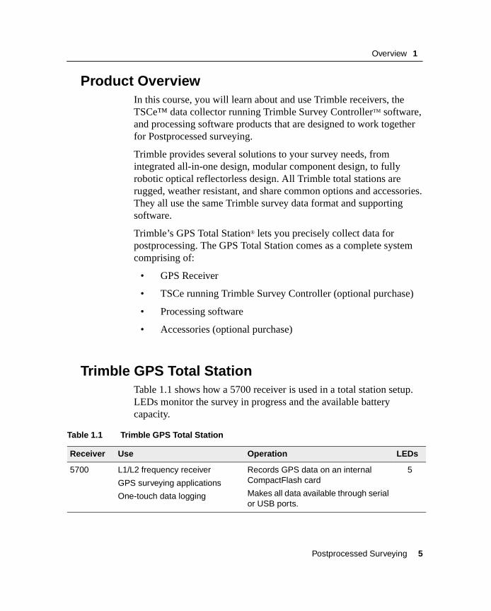
1.7 Trimble GPS Total StationTable 1.1 shows how a 5700 receiver is used in a total station setup. LEDs monitor the survey in progress and the available battery capacity.
Table 1.1 Trimble GPS Total Station
Receiver Use Operation LEDs
5700 L1/L2 frequency receiver
GPS surveying applications
One-touch data logging
Records GPS data on an internal CompactFlash card
Makes all data available through serial or USB ports.
5
Postprocessed Surveying 5

1 Overview
1.8 The TSCe Data Collector (TSCe)The TSCe running the Trimble Survey Controller software controls Trimble Postprocessed systems and makes surveying a faster and more efficient process. Trimble Survey Controller is the link between all Trimble GPS receivers and the office-based software suites. It is also links Trimble GPS/Conventional products to other existing optical total station products.
With the Trimble Survey Controller, you can:
• Configure instrument settings and data collection methods to best suit your requirements.
• Collect features and attributes according to a feature and attribute library that you define in the Trimble Geomatics Office™ software or within Trimble Survey Controller.
• Store external sensor data as attribute values, or combine them with GPS positions.
• Calculate areas, offsets, and intersections to points, lines, or arcs.
• Stakeout design or calculated features, including road templates and DTM.
• Communicate with other optical total station products.
• Monitor the status of your PPS system.
6 Postprocessed Surveying
Overview 1
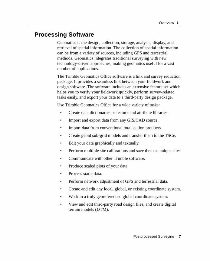
1.9 Processing SoftwareGeomatics is the design, collection, storage, analysis, display, and retrieval of spatial information. The collection of spatial information can be from a variety of sources, including GPS and terrestrial methods. Geomatics integrates traditional surveying with new technology-driven approaches, making geomatics useful for a vast number of applications.
The Trimble Geomatics Office software is a link and survey reduction package. It provides a seamless link between your fieldwork and design software. The software includes an extensive feature set which helps you to verify your fieldwork quickly, perform survey-related tasks easily, and export your data to a third-party design package.
Use Trimble Geomatics Office for a wide variety of tasks:
• Create data dictionaries or feature and attribute libraries.
• Import and export data from any GIS/CAD source.
• Import data from conventional total station products.
• Create geoid sub-grid models and transfer them to the TSCe.
• Edit your data graphically and textually.
• Perform multiple site calibrations and save them as unique sites.
• Communicate with other Trimble software.
• Produce scaled plots of your data.
• Process static data.
• Perform network adjustment of GPS and terrestrial data.
• Create and edit any local, global, or existing coordinate system.
• Work in a truly georeferenced global coordinate system.
• View and edit third-party road design files, and create digital terrain models (DTM).
Postprocessed Surveying 7

1 Overview
1.10 Trimble Resources
1.10.1 Internet
The Trimble website provides access to Trimble’s newest customer support tools. To obtain technical documents and utilities, access the website directly at http://www.trimble.com.
1.10.2 Product Training
For information about training on Trimble products, check the Trimble website or contact your local dealer.
1.10.3 Technical Assistance
If you have a problem and cannot find the information you need in the product documentation, check the Trimble website or contact your local dealer.
1.10.4 Contact Details
Trimble local dealer:
Company name
Phone number
Fax number
Contact person
8 Postprocessed Surveying

Overview 1
1.11 Other ResourcesThe following website provides GPS as well as control point information, primarily in the United States. For information about your region, ask your trainer.
1.11.1 U.S. Coast Guard (USCG)
This is a source for current GPS and satellite information, including information on the number of operational space vehicles (SVs), times and dates they will be available, and launch dates for new and replacement SVs.
U.S. Coast Guard website: www.navcen.uscg.gov/default.htm
Postprocessed Surveying 9

1 Overview
10 Postprocessed Surveying

C H A P T E R
2
GPS and Surveying 2In this chapter:
■ Introduction
■ Session objectives
■ The Global Positioning System
■ Satellite signal structure
■ GPS coordinate systems
■ Error sources in GPS
■ GPS surveying concepts
■ GPS surveying techniques
■ Techniques for survey tasks
■ Review questions
■ Answers

2 GPS and Surveying
2.1 IntroductionThis chapter introduces you to the Global Positioning System (GPS) and the concepts related to surveying with GPS.
2.2 Session ObjectivesAt the end of this session, you will be able to identify and explain the following GPS elements:
• Segments
• Satellite signal structure and observables
• Coordinate systems
• Sources of error in measurements
• Surveying concepts and techniques
12 Real-Time Kinematic Surveying
GPS and Surveying 2
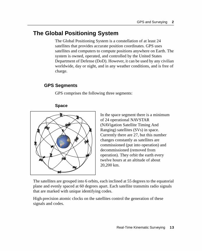
2.3 The Global Positioning SystemThe Global Positioning System is a constellation of at least 24 satellites that provides accurate position coordinates. GPS uses satellites and computers to compute positions anywhere on Earth. The system is owned, operated, and controlled by the United States Department of Defense (DoD). However, it can be used by any civilian worldwide, day or night, and in any weather conditions, and is free of charge.
2.3.1 GPS Segments
GPS comprises the following three segments:
Space
The satellites are grouped into 6 orbits, each inclined at 55 degrees to the equatorial plane and evenly spaced at 60 degrees apart. Each satellite transmits radio signals that are marked with unique identifying codes.
High-precision atomic clocks on the satellites control the generation of these signals and codes.
In the space segment there is a minimum of 24 operational NAVSTAR (NAVigation Satellite Timing And Ranging) satellites (SVs) in space. Currently there are 27, but this number changes constantly as satellites are commissioned (put into operation) and decommissioned (removed from operation). They orbit the earth every twelve hours at an altitude of about 20,200 km.
Real-Time Kinematic Surveying 13

2 GPS and Surveying
Control
The control segment is the “brain” of GPS. The United States Department of Defense (DoD) controls the system using a master station and four ground-based monitor/upload stations. Each satellite passes over a monitoring station twice a day.
• The monitor stations continuously track the satellites and provide this data to the master station.
• The master station is located at Schriever Air Force Base in Colorado Springs, Colorado, USA. The station calculates corrections to synchronize the atomic clocks aboard the satellites, and revises orbital information. It then forwards these results to the upload stations.
• The upload stations update each individual satellite using the information provided by the master station.
The master station, and monitor/upload stations are shown in Figure 2.1.
Figure 2.1 GPS master station, and the monitor/upload station network
Schriever AFB Colorado SpringsMaster Control Monitor Station
KwajaleinMonitor Station
HawaiiMonitor Station
Ascension IslandMonitor Station
Diego garciaMonitor Station
14 Real-Time Kinematic Surveying

GPS and Surveying 2
User
Anyone who has a GPS receiver can use GPS, and signals are used by civilians as well as by the military. Initially, GPS receivers were used mainly for position determination and navigation, but now they are used for a range of precise survey tasks on land, on sea, and in the air. Applications include surveying, agriculture, aviation, emergency services, recreation, and vehicle tracking.
For more information about GPS applications, visit the Trimble website (www.trimble.com). Civilian users currently outnumber military users.
Real-Time Kinematic Surveying 15
2 GPS and Surveying
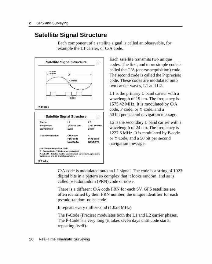
2.4 Satellite Signal StructureEach component of a satellite signal is called an observable, for example the L1 carrier, or C/A code.
C/A code is modulated onto an L1 signal. The code is a string of 1023 digital bits in a pattern so complex that it looks random, and so is called pseudorandom (PRN) code or noise.
There is a different C/A code PRN for each SV. GPS satellites are often identified by their PRN number, the unique identifier for each pseudo-random-noise code.
It repeats every millisecond (1.023 MHz)
The P-Code (Precise) modulates both the L1 and L2 carrier phases. The P-Code is a very long (it takes seven days until code starts repeating itself).
Satellite Signal Structure
Carrier L1 L2Frequency 1575.42 MHz 1227.60 MHzWavelength 19cm 24cm
Code Modulation C/A-code -P(Y)-code P(Y)-codeNAVDATA NAVDATA
C/A - Coarse Acquisition CodeP - Precise Code (Y-Code when encrypted)NAVDATA - Satellite health, satellite clock corrections, ephemerisparameters and SV orbital parameters.
Satellite Signal Structure
L1 = 19 cmL2 = 24 cm
Carrier
Code
λ
Each satellite transmits two unique codes. The first, and more simple code is called the C/A (coarse acquisition) code. The second code is called the P (precise) code. These codes are modulated onto two carrier waves, L1 and L2.
L1 is the primary L-band carrier with a wavelength of 19 cm. The frequency is 1575.42 MHz. It is modulated by C/A code, P-code, or Y-code, and a 50 bit per second navigation message.
L2 is the secondary L-band carrier with a wavelength of 24 cm. The frequency is 1227.6 MHz. It is modulated by P-code or Y-code, and a 50 bit per second navigation message.
16 Real-Time Kinematic Surveying
GPS and Surveying 2
When Anti-Spoofing is active, the P-Code is encrypted into theY-Code.
GPS receivers are single-frequency or dual-frequency.
Single-frequency receivers observe the L1 carrier wave, while dual-frequency receivers observe both the L1 and L2 carrier waves.
Navigation message contains system time, clock correction parameters, ionospheric delay model parameters, and details of the satellite’s ephemeris and health. The information is used to process GPS signals to obtain user position and velocity.
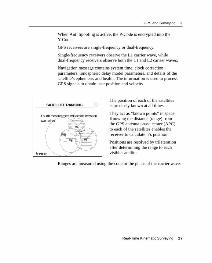
Ranges are measured using the code or the phase of the carrier wave.
SATELLITE RANGING
Fourth measurement will decide betweentwo points
The position of each of the satellites is precisely known at all times.
They act as “known points” in space. Knowing the distance (range) from the GPS antenna phase center (APC) to each of the satellites enables the receiver to calculate it’s position.
Positions are resolved by trilateration after determining the range to each visible satellite.
Real-Time Kinematic Surveying 17

2 GPS and Surveying
2.4.1 Satellite Range Based on Code Measurements
The GPS receiver has a C/A code generator that produces the same PRN code as the satellite does. Code received from the satellite is compared with the code generated by the receiver, sliding a replica of the code in time until there is correlation with the SV code, as shown in Figure 2.2.
Figure 2.2 Code measurements
There is a time difference between when the same part of the code is generated in the satellite and when it is received at the GPS antenna. Code measurements make it possible to record this time difference. The measurements are multiplied by the speed of light (speed at which GPS signal travels), so range can be determined.
Code range observables provide pseudorange time differences between satellites and a single autonomous receiver. The result of a code range is called the autonomous position.To obtain the autonomous position, only one receiver is required.This position may be used in baseline processing as an initial receiver starting position.
measure time differencebetween same part of code
From satellite
From ground receiver
18 Real-Time Kinematic Surveying

GPS and Surveying 2
2.4.2 Satellite Range Based on Carrier Phase Measurements
Survey-grade GPS receivers measure the difference in carrier phase cycles and fractions of cycles over time. At least two receivers track carrier phase, and any changes are recorded in both.
L1 and L2 wavelengths are known, so ranges are determined by adding the phase difference to the total number of waves that occur between each satellite and the antenna.
Carrier phase observables provide true range, the exact number of wavelengths from the antenna phase center to the satellite, between two receivers.
For postprocessed surveys, the WAVE™ Baseline processing module resolves the integer ambiguity and determines the integer during baseline postprocessing.
The Integer Ambiguity
∆λ∆λ∆λ∆λ
∆λ∆λ∆λ∆λ = First Partial Wavelength
NN = Integer Ambiguity
Solving for the IntegerAmbiguity yields
centimeter precision
Determining the full number of cycles between the antenna and the satellite is referred to as the integer ambiguity search.
Resolving the integer ambiguity is essential for surveys that require centimeter-level precision.
Real-Time Kinematic Surveying 19
2 GPS and Surveying
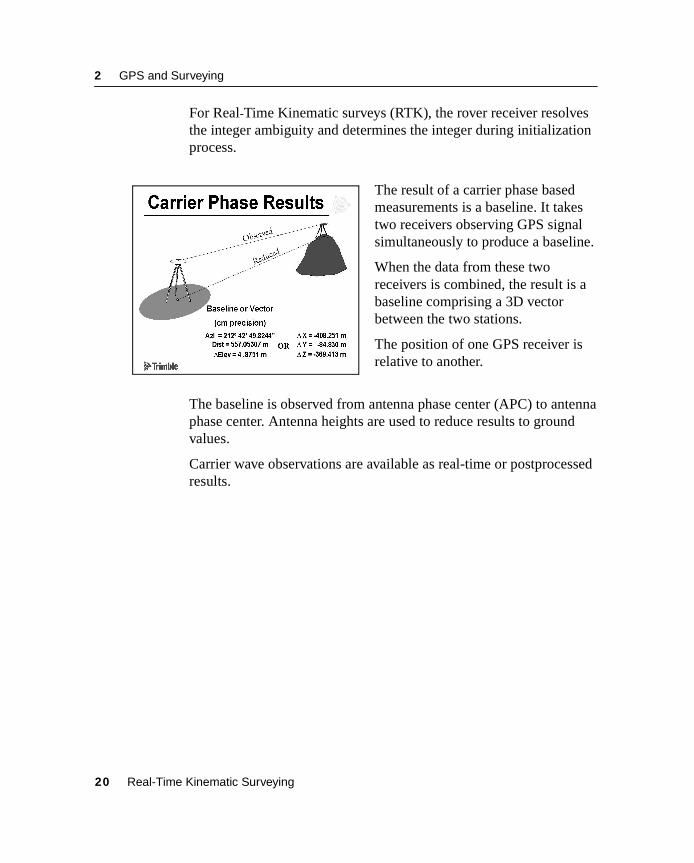
For Real-Time Kinematic surveys (RTK), the rover receiver resolves the integer ambiguity and determines the integer during initialization process.
The result of a carrier phase based measurements is a baseline. It takes two receivers observing GPS signal simultaneously to produce a baseline.
When the data from these two receivers is combined, the result is a baseline comprising a 3D vector between the two stations.
The position of one GPS receiver is relative to another.
The baseline is observed from antenna phase center (APC) to antenna phase center. Antenna heights are used to reduce results to ground values.
Carrier wave observations are available as real-time or postprocessed results.
20 Real-Time Kinematic Surveying

GPS and Surveying 2
2.5 GPS Coordinate SystemsThe GPS coordinate system is described in the following sections:
• Earth-Centered, Earth-Fixed
• Reference Ellipsoid
• ECEF and WGS-84
• Geoid and GPS Height
2.5.1 Earth-Centered, Earth-Fixed
ECEF Coordinate System
+Z
-Y
+X
XY
Z
ECEFX = -2691542.5437 mY = -4301026.4260 mZ = 3851926.3688 m
ECEF is a cartesian coordinate system used by the WGS-84 reference frame. In this coordinate system, the center of the system is at the earth’s center of mass. The z-axis is coincident with the mean rotational axis of the earth and the x-axis passes through 0° N and 0° E. The y-axis is perpendicular to the plane of the x- and z-axes. All axes are fixed to the earth’s motion.
Real-Time Kinematic Surveying 21
2 GPS and Surveying
2.5.2 Reference Ellipsoid
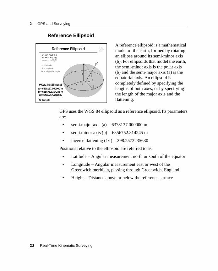
GPS uses the WGS-84 ellipsoid as a reference ellipsoid. Its parameters are:
• semi-major axis (a) = 6378137.000000 m
• semi-minor axis (b) = 6356752.314245 m
• inverse flattening (1/f) = 298.2572235630
Positions relative to the ellipsoid are referred to as:
• Latitude – Angular measurement north or south of the equator
• Longitude – Angular measurement east or west of the Greenwich meridian, passing through Greenwich, England
• Height – Distance above or below the reference surface
Reference Ellipsoid
a
b
a = semi-major axisb = semi-minor axis
Flattening f(a b)
a=
−
b
a λφ
Hφλ
latitude
longitude
H ellipsoidal height
≡≡≡
WGS-84 Ellipsoida = 6378137.000000 mb = 6356752.314245 m1/f = 298.2572235630
A reference ellipsoid is a mathematical model of the earth, formed by rotating an ellipse around its semi-minor axis (b). For ellipsoids that model the earth, the semi-minor axis is the polar axis (b) and the semi-major axis (a) is the equatorial axis. An ellipsoid is completely defined by specifying the lengths of both axes, or by specifying the length of the major axis and the flattening.
22 Real-Time Kinematic Surveying

GPS and Surveying 2
2.5.3 ECEF and WGS-84
The model takes into account the size and shape of the ellipsoid, and the location of the center of the ellipsoid with respect to the center of the earth (a point on the topographic surface established as the origin of the datum).
All GPS coordinates are based on the WGS-84 datum surface.
The WGS-84 geodetic datum is a mathematical model designed to fit part or all of the geoid (the physical earth’s surface). A geodetic datum is defined by the relationship between an ellipsoid and the center of the earth. For ECEF and WGS-84, mathematical conversions can be calculated between the two reference systems.
ECEF and WGS-84
+Z
-Y
+X
ECEFX = -2691542.5437 mY = -4301026.4260 mZ = 3851926.3688 m
XY
Z
b
aλ
φ
H
WGS-84φ φ φ φ = 37o 23’ 26.38035” N
λλλλ = 122o 02’ 16.62574” WH = -5.4083 m
Real-Time Kinematic Surveying 23
2 GPS and Surveying
2.5.4 Geoid and GPS Height
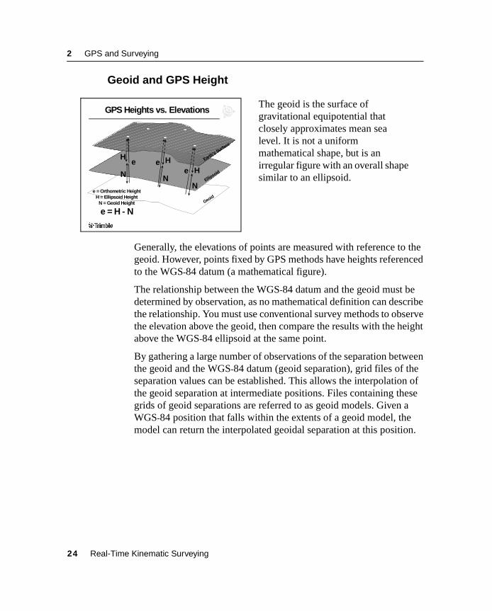
Generally, the elevations of points are measured with reference to the geoid. However, points fixed by GPS methods have heights referenced to the WGS-84 datum (a mathematical figure).
The relationship between the WGS-84 datum and the geoid must be determined by observation, as no mathematical definition can describe the relationship. You must use conventional survey methods to observe the elevation above the geoid, then compare the results with the height above the WGS-84 ellipsoid at the same point.
By gathering a large number of observations of the separation between the geoid and the WGS-84 datum (geoid separation), grid files of the separation values can be established. This allows the interpolation of the geoid separation at intermediate positions. Files containing these grids of geoid separations are referred to as geoid models. Given a WGS-84 position that falls within the extents of a geoid model, the model can return the interpolated geoidal separation at this position.
GPS Heights vs. Elevations
NNN
e ee
H HH
Earth’s Surfa
ce
Ellipsoid
Geoide = Orthometric Height
H = Ellipsoid HeightN = Geoid Height
e = H - N
The geoid is the surface of gravitational equipotential that closely approximates mean sea level. It is not a uniform mathematical shape, but is an irregular figure with an overall shape similar to an ellipsoid.
24 Real-Time Kinematic Surveying
GPS and Surveying 2
2.6 Error Sources in GPSMeasurement errors can never be completely eliminated. This section explains the following sources of errors in GPS:
• Satellite geometry
• Human error
• Selective Availability (SA) and Anti-Spoofing (AS)
• Atmospheric effects
• Multipath
2.6.1 Satellite Geometry
Dilution of Precision (DOP) is an indicator of the quality of a GPS position.
It is a unitless figure of merit expressing the relationship between the error in user position and the error in satellite position. It takes into account the location of each satellite relative to other satellites in the constellation, as well as their geometry relative to the GPS receiver.
PDOP is inversely proportional to the volume of the pyramid formed by lines running from the receiver to four satellites observed.
Values considered good for positioning are small (for example, 3). Values greater than 7 are considered poor. Small PDOP is associated with widely separated satellites.
PDOP is related to horizontal and vertical DOP by:
PDOP2 =HDOP2 +VDOP2.
A low DOP value indicates a higher probability of accuracy.
Standard DOPs for GPS applications are:
• PDOP – Position Dilution of Precision (three coordinates)
• RDOP – Relative Dilution of Precision (Position, averaged over time)
Real-Time Kinematic Surveying 25

2 GPS and Surveying
• HDOP – Horizontal Dilution of Precision (two horizontal coordinates)
• VDOP – Vertical Dilution of Precision (height only)
• TDOP – Time Dilution of Precision (clock offset only)
• GDOP – Geometric Dilution of Precision. (The relationship between errors in user position and time, and errors in satellite range).
Good Satellite GeometryGood PDOP occurs when the satellites are geometrically balanced above your position.
Poor Satellite GeometryGPS precision is diluted, leading to poor PDOP, when satellites are not balanced. Poor PDOP may occur:
• even when you have a large number of satellites, if they are in a line
• when all satellites are positioned directly overhead or all are in one cluster in the sky
26 Real-Time Kinematic Surveying

GPS and Surveying 2
The PDOP mask is a user-definable setting used to limit the effects of SV geometry on the accuracy of GPS position. It is the highest PDOP value at which a receiver will compute positions.
2.6.2 Human Error
Human error is typically the greatest contributor of error. Some examples include:
• Misreading antenna height measurements
• Transposing numbers
• Rushing observations and shortening observation times
• Poor centering and leveling over points
2.6.3 SA and AS
The Department of Defense (DoD, USA) controls Selective Availability (SA) and Anti-Spoofing (AS).
Selective Availability – SA was a purposely-introduced artificial degradation of the GPS satellite signal. It involved distorting the information about SV location and time, two main components in calculating the receiver’s position. The magnitude of the error in autonomous GPS introduced by the SA was 100 m (H) and 156 m (V).
Selective Availability was turned off on 1 May 2000.
The error in autonomous GPS position since discontinuation of SA is approximately 8–10 m (H) and 10–15 m (V).
Anti-Spoofing – AS allows transmitting of an encrypted Y-code in place of P-code. Y-code is intended to be useful only to authorized (primarily military) users. AS is used to deny the full precision of GPS to civilian users.
Real-Time Kinematic Surveying 27
2 GPS and Surveying
2.6.4 Atmospheric Effects
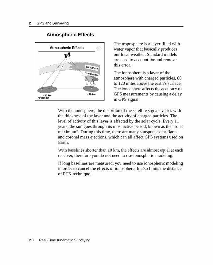
With the ionosphere, the distortion of the satellite signals varies with the thickness of the layer and the activity of charged particles. The level of activity of this layer is affected by the solar cycle. Every 11 years, the sun goes through its most active period, known as the “solar maximum”. During this time, there are many sunspots, solar flares, and coronal mass ejections, which can all affect GPS systems used on Earth.
With baselines shorter than 10 km, the effects are almost equal at each receiver, therefore you do not need to use ionospheric modeling.
If long baselines are measured, you need to use ionospheric modeling in order to cancel the effects of ionosphere. It also limits the distance of RTK technique.
The troposphere is a layer filled with water vapor that basically produces our local weather. Standard models are used to account for and remove this error.
The ionosphere is a layer of the atmosphere with charged particles, 80 to 120 miles above the earth’s surface. The ionosphere affects the accuracy of GPS measurements by causing a delay in GPS signal.
Troposphere
Atmospheric Effects
Ionosphere
< 10 km > 10 km
28 Real-Time Kinematic Surveying
GPS and Surveying 2
2.6.5 Multipath
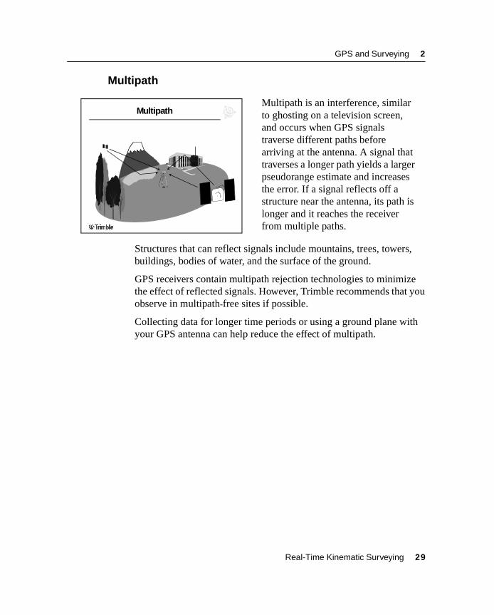
Structures that can reflect signals include mountains, trees, towers, buildings, bodies of water, and the surface of the ground.
GPS receivers contain multipath rejection technologies to minimize the effect of reflected signals. However, Trimble recommends that you observe in multipath-free sites if possible.
Collecting data for longer time periods or using a ground plane with your GPS antenna can help reduce the effect of multipath.
MultipathMultipath is an interference, similar to ghosting on a television screen, and occurs when GPS signals traverse different paths before arriving at the antenna. A signal that traverses a longer path yields a larger pseudorange estimate and increases the error. If a signal reflects off a structure near the antenna, its path is longer and it reaches the receiver from multiple paths.
Real-Time Kinematic Surveying 29
2 GPS and Surveying
2.7 GPS Surveying ConceptsGPS surveying requires the simultaneous observation of the same four (or more) satellites by at least two GPS receivers. Although you can use more than two receivers for some surveys, this manual limits discussion to the use of two: the base receiver and a rover receiver.
The base receiver is located over a known control point for the duration of the survey. The rover receiver is moved to the points that are to be surveyed or staked out. When the data from these two receivers is combined, the result is a 3D vector (baseline) between the base antenna phase center (APC) and the rover antenna phase center.
You can use different observation techniques to determine the position of the rover receiver relative to the base. These techniques are categorized according to the time at which a solution is made available:
• Real-time techniques use a radio to transmit base observations to the rover for the duration of the survey. As each measurement is completed, the solution is resolved.
• Postprocessed techniques require data to be stored and resolved some time after the survey has been completed.
Generally, the technique you choose depends on factors such as the receiver configuration, the accuracy required, time constraints, and whether or not you need real-time results.
30 Real-Time Kinematic Surveying
GPS and Surveying 2
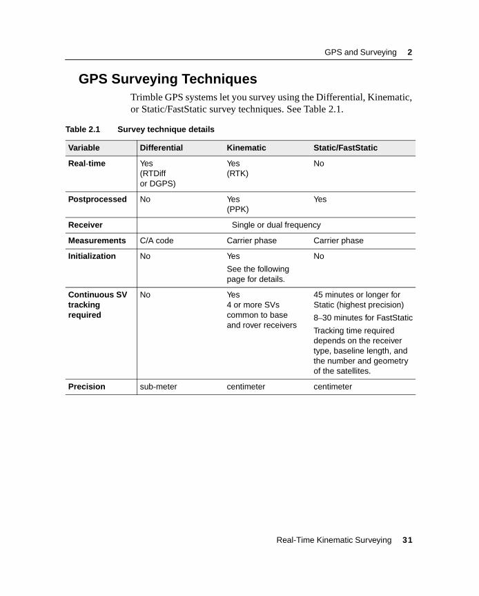
2.8 GPS Surveying TechniquesTrimble GPS systems let you survey using the Differential, Kinematic, or Static/FastStatic survey techniques. See Table 2.1.
Table 2.1 Survey technique details
Variable Differential Kinematic Static/FastStatic
Real-time Yes (RTDiff or DGPS)
Yes (RTK)
No
Postprocessed No Yes (PPK)
Yes
Receiver Single or dual frequency
Measurements C/A code Carrier phase Carrier phase
Initialization No Yes
See the following page for details.
No
Continuous SV tracking required
No Yes 4 or more SVs common to base and rover receivers
45 minutes or longer for Static (highest precision)
8–30 minutes for FastStatic
Tracking time required depends on the receiver type, baseline length, and the number and geometry of the satellites.
Precision sub-meter centimeter centimeter
Real-Time Kinematic Surveying 31

2 GPS and Surveying
2.8.1 Kinematic Survey Initialization
To achieve the required precision, RTK and PPK surveys must first be initialized:
• 5700 for Real Time Survey – Set the rover over a known or a new point. Initialization can also be achieved while the rover is moving.
• 5700 receiver for postprocessed surveys – OTF initializations begin once the survey is started
Note – If the number of common satellites falls below four while you are surveying, the survey must be reinitialized when four or more satellites are again being tracked.
32 Real-Time Kinematic Surveying

GPS and Surveying 2
2.9 Techniques for Survey TasksSurveyors use GPS for control surveys, topographic surveys, and stakeout.
2.9.1 Control Surveys
Control surveys establish control points in a region of interest. Baselines are measured using careful observation techniques. These baselines form tightly braced networks, and precise coordinates result from the rigorous adjustment of the networks. Static and FastStatic observation techniques, combined with a network adjustment, are best suited to control work.
2.9.2 Topographic Surveys
Topographic surveys determine the coordinates of significant points in a region of interest. They are usually used to produce maps.
Kinematic techniques (real-time or postprocessed) are best suited to topographic surveys because of the short occupation time required for each point.
2.9.3 Stakeout
Stakeout is the procedure whereby predefined points are located and marked. To stake out a point, you need results in real time. Real-Time Kinematic (RTK) is the only technique that provides centimeter-level, real-time solutions.
Real-Time Kinematic Surveying 33
2 GPS and Surveying
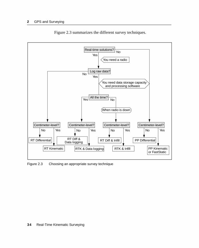
Figure 2.3 summarizes the different survey techniques.
Figure 2.3 Choosing an appropriate survey technique
Real-time solutions?
Centimeter-level? Centimeter-level?Centimeter-level?Centimeter-level?
Log raw data?
You need a radio
You need data storage capacityand processing software
All the time?
RT Differential
RT Kinematic
When radio is down
YesNo
NoYes
NoYes
Yes No
PP Differential
PP Kinematic
YesNo
RT Diff & Infill
RTK & Infill
YesNo
RT Diff &
RTK & Data logging
YesNo
or FastStatic
Data logging
34 Real-Time Kinematic Surveying

GPS and Surveying 2
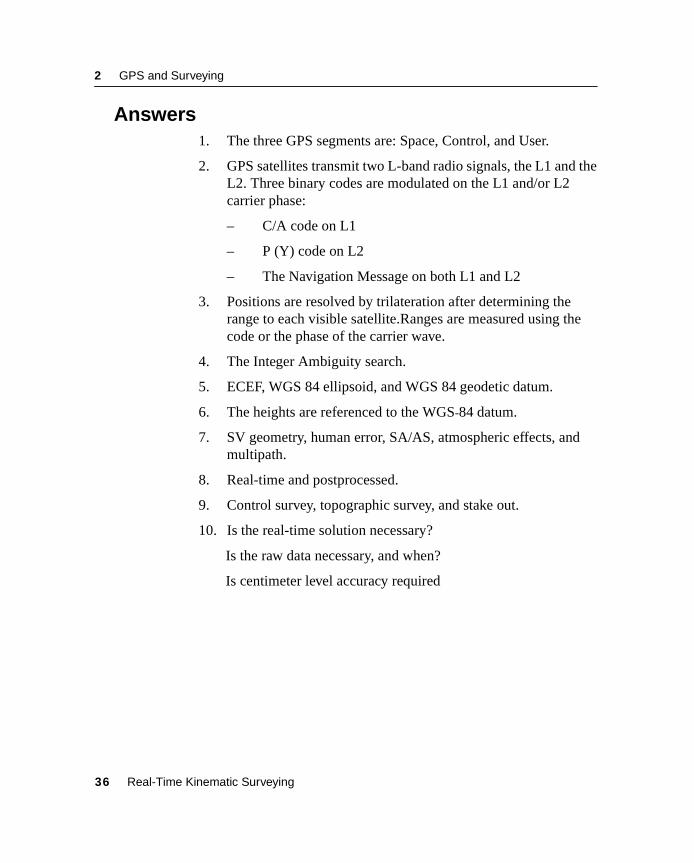
2.10 Review QuestionsThese questions test what you have learned about the Global Positioning System and GPS surveying requirements:
1. What are the three segments of GPS?
2. What is the structure of the GPS signal?
3. How is the GPS receiver position determined?
4. Determining the full number of carrier phase cycles between the GPS antenna and the SV is commonly called?
5. Name the following: GPS coordinate system, GPS reference ellipsoid and GPS geodetic datum.
6. When measuring with GPS, to what surface are the heights referenced?
7. What are the error sources in GPS measurement?
8. How are GPS observation techniques categorized based on the time at which a solution is made available?
9. What survey tasks is GPS used for?
10. What should you consider when choosing an appropriate observation technique?
Real-Time Kinematic Surveying 35
2 GPS and Surveying
2.11 Answers1. The three GPS segments are: Space, Control, and User.
2. GPS satellites transmit two L-band radio signals, the L1 and the L2. Three binary codes are modulated on the L1 and/or L2 carrier phase:
– C/A code on L1
– P (Y) code on L2
– The Navigation Message on both L1 and L2
3. Positions are resolved by trilateration after determining the range to each visible satellite.Ranges are measured using the code or the phase of the carrier wave.
4. The Integer Ambiguity search.
5. ECEF, WGS 84 ellipsoid, and WGS 84 geodetic datum.
6. The heights are referenced to the WGS-84 datum.
7. SV geometry, human error, SA/AS, atmospheric effects, and multipath.
8. Real-time and postprocessed.
9. Control survey, topographic survey, and stake out.
10. Is the real-time solution necessary?
Is the raw data necessary, and when?
Is centimeter level accuracy required
36 Real-Time Kinematic Surveying

C H A P T E R
3
Postprocessed Surveying Systems 3In this chapter:
■ Introduction
■ Session objectives
■ Postprocessed surveying (PPS) overview
■ Initialization (resolving the integer ambiguity)
■ PPS system components
■ Assembling a postprocessed survey system
■ General guidelines
■ Measuring GPS antenna heights
■ PPS system equipment checklist
■ Use and Care
■ General guidelines
■ Review questions
■ Answers

3 Postprocessed Surveying Systems
3.1 IntroductionThis chapter gives an overview of Postprocessed Surveying (PPS), including survey concepts and requirements, and equipment checklists, connection diagrams, and use and care information.
3.2 Session ObjectivesAt the end of this session, you will know:
• The fundamental concepts and requirements for performing a Postprocessed survey
• How to assemble a PPS System
• The importance of proper use and care for the equipment
38 Postprocessed Surveying

Postprocessed Surveying Systems 3
3.3 Postprocessed Surveying (PPS) OverviewPostprocessed surveys are surveys in which data is collected in the field and data processing occurs at the later stage, using the Trimble Geomatics Office software.
Postprocessed kinematic surveys can include stop-and-go data collection and continuous data collection.
The two GPS receivers used in a PPS survey must:
• Observe and track carrier phase measurements
• Log data at common times and epochs
• Track four common satellites at each location
• Observe during good satellite (SV) geometry (DOP)
The requirements for Postprocessed Kinematic (PPK) surveying include:
• Initialization
• Maintaining lock to satellites while moving
It is possible to achieve centimeter, or better, precision with PPS, depending on which of the following techniques of data collection is used:
• Static
• FastStatic
• Kinematic, Postprocessed (PPK)
Postprocessed Surveying 39

3 Postprocessed Surveying Systems
3.3.1 Static Surveying/FastStatic Surveying
Static
Static surveying is the most precise GPS surveying technique and can be performed with either single-frequency or dual-frequency receivers. Applications for Static surveying vary from primary geodetic control to high-precision surveys.
Like all GPS surveys, the Static survey requires the use of at least two receivers: one receiver at each point defining the baseline, each logging observations simultaneously from at least four common satellites. You can increase productivity by using more receivers, however, Network design dictates the sequence of observations.
Static surveying requires that observations be logged at each station for an extended period of time, usually about 45-60 minutes. Although this technique requires more time than others, a large amount of data collected allows the processing software to resolve more problems in the data set. This leads to greater precision in the baseline solution.
The information associated with each Static occupation is stored in its own data file. If the receiver is turned off in the middle of an occupation, you can open a second file and continue the survey. In this case, there is more than one file per occupation, but still only one occupation per file.
40 Postprocessed Surveying

Postprocessed Surveying Systems 3
FastStatic
FastStatic surveying is a data collection technique similar to Static surveying. It requires simultaneous observations of four or more satellites for a period of 8 or more minutes and yields baseline components with a precision similar to that of the Static technique. The length of time the receivers log data depends on the number and geometry (PDOP) of satellites being tracked, and the quality of the data being logged.
Cycle slips, multipath, and radio frequency (RF) interference can adversely affect data quality. In general, occupation times for FastStatic surveys on baselines of less than 20 km vary from about 8 minutes (when data is logged from at least 6 satellites) to about 20 minutes (with data from 4 satellites).
FastStatic surveying is similar to Static surveying in that data is logged only while the receiver is stationary and occupying a point. As the receiver moves from one point to another in the survey, the GPS receiver can be turned off as no data is logged.
The manner in which the data is treated by the baseline processor is also similar.
FastStatic surveying differs from Static surveying in that occupation times are shorter and less data is collected. Because the occupation time is shorter, resulting in fewer measurements for the baseline processor to use, FastStatic surveying requires more careful planning of data collection sessions. The expected baseline precision for Static is lower than that.
The other significant difference is the file management. Static surveying keeps each occupation in its own data file; FastStatic surveying contains all occupations in one data file.
Postprocessed Surveying 41
3 Postprocessed Surveying Systems
3.3.2 Postprocessed Kinematic (PPK) Surveying
Many field techniques used in Postprocess Kinematic (PPK) surveying are different from Static and FastStatic. However, the processing and underlying theory are similar. The hardware required is the same as for Static and FastStatic surveying.
Static and FastStatic techniques do not require initialization, while PPK does. The purpose of initialization is to collect enough data so that the WAVE baseline processor in Trimble Geomatics Office can resolve the integer ambiguity from the GPS signal.
Once initialization is gained, it does not change as long as the receiver maintains lock on the satellites. The WAVE baseline processor applies the integer ambiguity solution to subsequent solutions. Therefore, after initialization, you only need an occupation time that records enough data to derive new coordinates.
If satellite signal loss occurs, a new initialization is required.
Kinematic surveying is mostly used for topographic surveying, where rapid data collection is required without the Static/FastStatic level of accuracy.
The main advantage of the method is that after initialization, you can use short occupation times (1–30 seconds) to obtain 1–2 cm precisions.
42 Postprocessed Surveying
Postprocessed Surveying Systems 3
3.4 Initialization (Resolving the Integer Ambiguity)This section explains initialization, or how to establish an exact position by calculating the difference between carrier phase signals received by the base and rover receivers.
The carrier phase observable of the received GPS satellite signal is used to measure satellite range, and is responsible for achieving centimeter level accuracy. These range measurements are used to compute baselines between the base APC and rover APC.
But what exactly is a carrier phase measurement? Why is it referred to as ambiguous? And how is the ambiguity resolved via initialization?
To answer these questions, see the following sections on phase measurement, carrier phase differencing, ambiguity resolution, and baseline solutions.
Note – With PPK surveys, initialization is computed by the WAVE Baseline Processing module of the Trimble Geomatics Office software. Enough data has to be collected during the field data collection to enable software computations. For more information, see Initialization Methods, page 47.
Postprocessed Surveying 43

3 Postprocessed Surveying Systems
3.4.1 Phase Measurement
The GPS carrier wave is a right-circularly polarized wave. Phase measurements occur as follows:
1. The first measurement observed is a partial phase of the GPS carrier.
2. After this partial phase, the receiver measures whole wavelengths of the carrier wave.
3. The receiver continuously counts whole wavelengths. The receiver does not know (ambiguous) the exact number of whole wavelengths (integer) between the SV and GPS APC.
Phase Measurement
12
39
6
∆λ∆λ∆λ∆λ
Continuous CarrierPhase Measurement
44 Postprocessed Surveying
Postprocessed Surveying Systems 3
3.4.2 Carrier Phase Differencing
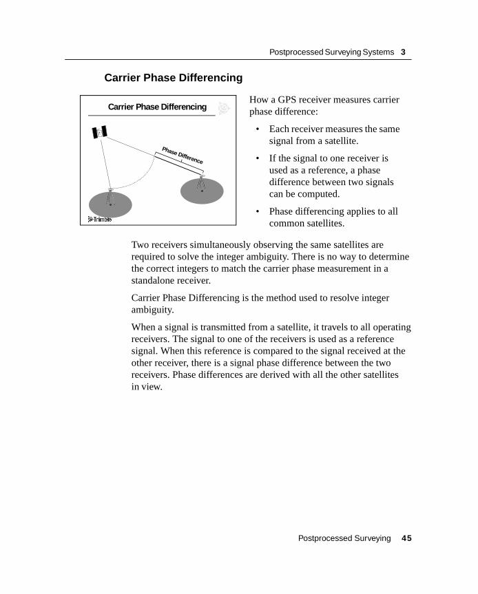
Two receivers simultaneously observing the same satellites are required to solve the integer ambiguity. There is no way to determine the correct integers to match the carrier phase measurement in a standalone receiver.
Carrier Phase Differencing is the method used to resolve integer ambiguity.
When a signal is transmitted from a satellite, it travels to all operating receivers. The signal to one of the receivers is used as a reference signal. When this reference is compared to the signal received at the other receiver, there is a signal phase difference between the two receivers. Phase differences are derived with all the other satellites in view.
Carrier Phase Differencing
Phase Difference
How a GPS receiver measures carrier phase difference:
• Each receiver measures the same signal from a satellite.
• If the signal to one receiver is used as a reference, a phase difference between two signals can be computed.
• Phase differencing applies to all common satellites.
Postprocessed Surveying 45
3 Postprocessed Surveying Systems
3.4.3 Ambiguity Resolution
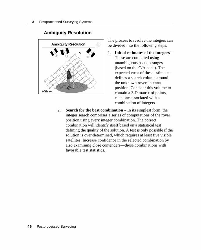
The process to resolve the integers can be divided into the following steps:
1. Initial estimates of the integers – These are computed using unambiguous pseudo ranges (based on the C/A code). The expected error of these estimates defines a search volume around the unknown rover antenna position. Consider this volume to contain a 3-D matrix of points, each one associated with a combination of integers.
2. Search for the best combination – In its simplest form, the integer search comprises a series of computations of the rover position using every integer combination. The correct combination will identify itself based on a statistical test defining the quality of the solution. A test is only possible if the solution is over-determined, which requires at least five visible satellites. Increase confidence in the selected combination by also examining close contenders—those combinations with favorable test statistics.
Ambiguity Resolution
λλλλ
46 Postprocessed Surveying

Postprocessed Surveying Systems 3
3.4.4 Float and Fixed Solutions
Before enough data is collected for WAVE to resolve the integer ambiguities, the PPK survey solution type is known as a float solution.
Once enough data is collected, WAVE can resolve the integer ambiguities, and the PPK survey is said to be initialized. The solution becomes a fixed solution.
Note – PPK=FIX messages on the Trimble Survey Controller status bar does not mean that integer ambiguity is resolved. It simply indicates that enough data has been collected so integer ambiguities can be resolved by the WAVE.
3.4.5 Initialization Methods
There are four methods of initialization:
• Known Point – Requires a previously observed WGS-84 position or a known ground coordinate position.
• New Point – Allows you to calculate the initialization on a short-term static observation.
• Postprocessed On-the-Fly (OTF) – Allows you to compute the initialization while in motion.
Initialization methods are discussed in detail in Chapter 6, Field Procedures.
Postprocessed Surveying 47

3 Postprocessed Surveying Systems
3.4.6 Compute Baseline Solution
3. Determine a precise range to all common satellites to provide your roving position.
4. Provide the fixed (known) base position and the base station observations.
5. Calculate the baseline and check the inverse between the base and rover positions.
Note – In postprocessed surveys, the WAVE module of the Trimble Geomatics office software computes the baselines.
Compute Baseline Solution
37o 23’ 28.607434” N122o 02’ 41.161474” W
-12.637 m
37o 23’ 30.195065” N122o 02’ 33.948394” W
-12.445 m
Once the integer ambiguity is resolved, the baseline is computed to establish the rover’s APC position in relation to the base APC.
The process of computing the baseline solutions:
1. Compute the phase differencing.
2. Solve and apply the integer ambiguity to phase differences.
48 Postprocessed Surveying

Postprocessed Surveying Systems 3
3.5 PPS System Components
The GPS base station and each GPS rover must contain:
• GPS receiver
• GPS antenna
• Trimble Survey Controller (Postprocessed Kinematic surveys always require a TSCe at the rover receiver)
• Power supply (AC power supply or portable batteries)
• Appropriate cabling
A PPS system comprises these basic physical components:
• GPS base station
• GPS rover(s)
• TSCe running Trimble Survey Controller (optional)
Postprocessed Surveying 49
3 Postprocessed Surveying Systems
Base Station (Static/FastStatic or PPK base setup)
A Base station provides known coordinates for the relative positioning of the rover stations. It is set on a known point.
Typically, a Static/FastStatic or PPK base station consists of:
• Trimble GPS receiver
• TSCe running Trimble Survey Controller (optional)
• Stable observation position (tripod and tribrach or pillar)
• Power supply (AC power supply or portable batteries)
• Cables to connect the base station components
You can use the GPS receiver front panel to start your Postprocessed base station, or TSCe running Trimble Survey Controller. Ancillary Trimble programs, such as Trimble’s Reference Station (TRS™), GPS Configurator or Remote Controller can be also used.
Rover (Static/FastStatic rover setup)
Roving stations are used to survey positions relative to the base station. Typically, Static/FastStatic roving station(s) configuration is identical to Static/FastStatic base station configuration.
Rover (PPK rover setup)
A roving station consists of:
• Trimble 5700 GPS receiver and GPS antenna
• TSCe running Trimble Survey Controller
• Range pole and backpack (one of several models)
• Power supply (portable batteries)
• Cables to connect the rover components
50 Postprocessed Surveying

Postprocessed Surveying Systems 3
3.6 Assembling a Postprocessed Survey SystemThis section shows how to assemble the base station and rover receiver for a Static/FastStatic or PPK postprocessed survey.
Postprocessed Surveying 51
3 Postprocessed Surveying Systems
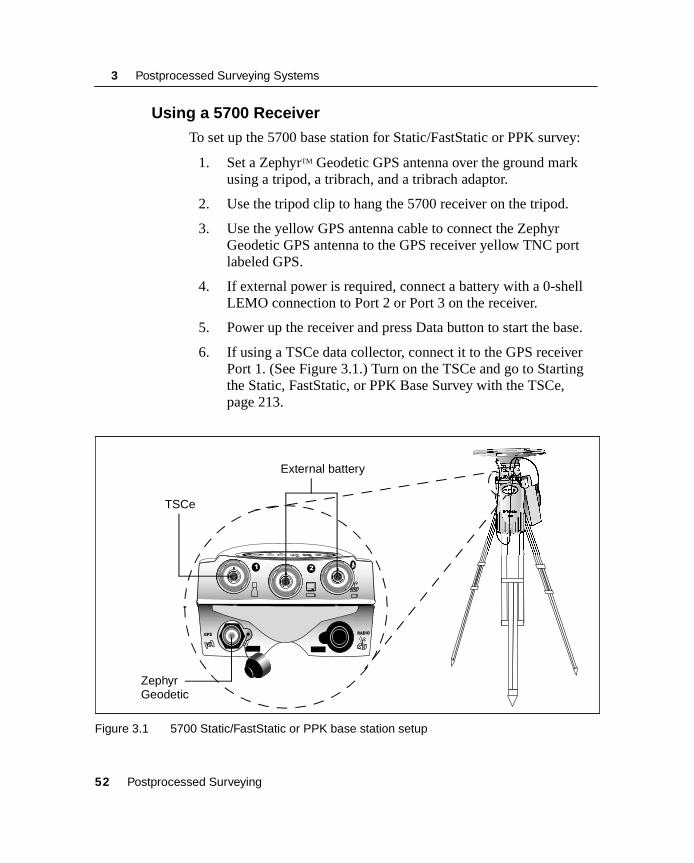
3.6.1 Using a 5700 Receiver
To set up the 5700 base station for Static/FastStatic or PPK survey:
1. Set a ZephyrTM Geodetic GPS antenna over the ground mark using a tripod, a tribrach, and a tribrach adaptor.
2. Use the tripod clip to hang the 5700 receiver on the tripod.
3. Use the yellow GPS antenna cable to connect the Zephyr Geodetic GPS antenna to the GPS receiver yellow TNC port labeled GPS.
4. If external power is required, connect a battery with a 0-shell LEMO connection to Port 2 or Port 3 on the receiver.
5. Power up the receiver and press Data button to start the base.
6. If using a TSCe data collector, connect it to the GPS receiver Port 1. (See Figure 3.1.) Turn on the TSCe and go to Starting the Static, FastStatic, or PPK Base Survey with the TSCe, page 213.
Figure 3.1 5700 Static/FastStatic or PPK base station setup
1 2
GPS RADIO
ZephyrGeodetic
TSCe
External battery
52 Postprocessed Surveying

Postprocessed Surveying Systems 3
To set up the 5700 rover for PPK survey:
1. Attach the Zephyr GPS antenna to the range pole.
2. Assemble 5700 GPS receiver on a pole or in a backpack.
3. Connect the Zephyr GPS antenna to the GPS receiver yellow TNC port labeled GPS.
4. Connect the TSCe to the GPS receiver Port labeled PORT 1. (See Figure 3.2.) Use the 0-shell LEMO to 0-shell LEMO cable.
5. Turn on the TSCe and go to Starting the PPK Rover Survey, page 221.
Figure 3.2 5700 PPK rover setup
Del
98
5 6
32
, Ctrl
Esc+_*/Copy
A B C D E F
G H I J
PONM
S T U V W X
K L
Q R
CutPaste
UndoMic
Y Z \
2 3
t
1 2
GPS RADIO
Zephyr antenna
Hand grip
Zephyrantenna
TSCe
External battery
Postprocessed Surveying 53
3 Postprocessed Surveying Systems
3.7 General GuidelinesThe following section gives guidelines for setting up a PPS system.
3.7.1 Setting Up the Base Station
Locate the base station where there is a clear and unobstructed view of the sky, for example, on top of a hill or building. You should be able to see the sky all around at an elevation angle of 13° above the horizon.
The WGS-84 coordinates for the base station should be known. Every 10 m error in these coordinates can cause an error of 1 ppm in the length of the RTK baseline. Define the coordinates in one of the following ways (the most accurate methods are listed first):
• Transfer or key in published WGS-84 coordinates.
• Transfer or key in WGS-84 coordinates derived from a previous control survey.
• Transfer or key in known grid coordinates, if a projection and datum transformation are known.
• Transfer or key in local geodetic coordinates, if a datum transformation is known.
• Use the ) softkey to obtain a WAAS position generated by the receiver. (North America only)
• Use the ) softkey to obtain the current approximate (autonomous) position calculated by the receiver. This position can be in error by up to 20 m, so you should perform a calibration to reduce the effect of this process.
Note – Only use an autonomous position once for each job—to start the first base receiver. (An autonomous position is equivalent to an assumed coordinate in conventional surveying.) This ensures that all surveys in the same job are in terms of each other. For base set-ups after day one, select your base position form the points stored in Trimble Survey Controller.
54 Postprocessed Surveying
Postprocessed Surveying Systems 3
3.7.2 Optimizing Field Equipment Setup
To become productive quickly when starting a survey, consider the following:
• Base station environment – Prior to setup you must be aware of the surveying environment. Whenever possible, set your base station to view the greatest amount of open sky so that it can maximize the satellite signal reception. Be aware of likely multipath sources such as buildings, wire fences, high voltage power sources, and trees.
• Ambient orientation – Both the base and the roving receivers require some time (approximately 2 minutes) to locate and lock onto satellite signals. This ambient time can be minimized by connecting the GPS antenna and power to the GPS receiver and allowing the antenna to view the open sky. You may simply rest your antenna equipment to one side while setting up the other necessary equipment for your base station or roving stations.
• Roving station environment – Move away from problem environments to avoid loss of lock (satellite tracking) or initialization for your roving receiver.
To detect the effects of a signal-limiting source:
– Check the number of currently tracked satellites at the rover and base using TSCe Instrument / Satellites menu.
– Monitor the root mean square (RMS) value of your present position. If the values exceed 70, move away from the problem environment.
B Tip – Although your base station will not be moving, you can detect the RMS values at your base when a job has been started with your TSCe. An RMS value of 30 indicates a low multipath environment.
Postprocessed Surveying 55
3 Postprocessed Surveying Systems
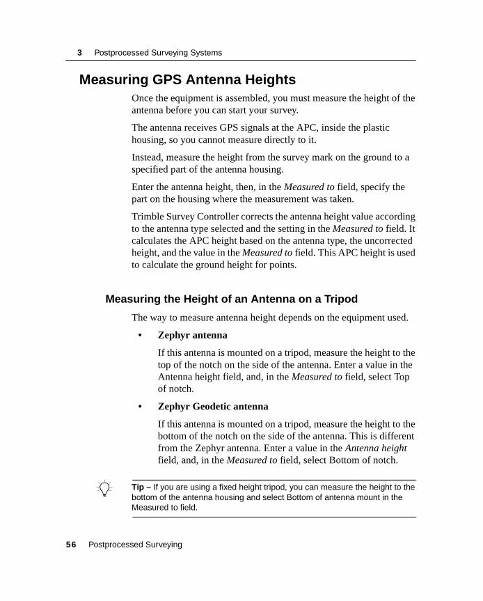
3.8 Measuring GPS Antenna HeightsOnce the equipment is assembled, you must measure the height of the antenna before you can start your survey.
The antenna receives GPS signals at the APC, inside the plastic housing, so you cannot measure directly to it.
Instead, measure the height from the survey mark on the ground to a specified part of the antenna housing.
Enter the antenna height, then, in the Measured to field, specify the part on the housing where the measurement was taken.
Trimble Survey Controller corrects the antenna height value according to the antenna type selected and the setting in the Measured to field. It calculates the APC height based on the antenna type, the uncorrected height, and the value in the Measured to field. This APC height is used to calculate the ground height for points.
3.8.1 Measuring the Height of an Antenna on a Tripod
The way to measure antenna height depends on the equipment used.
• Zephyr antenna
If this antenna is mounted on a tripod, measure the height to the top of the notch on the side of the antenna. Enter a value in the Antenna height field, and, in the Measured to field, select Top of notch.
• Zephyr Geodetic antenna
If this antenna is mounted on a tripod, measure the height to the bottom of the notch on the side of the antenna. This is different from the Zephyr antenna. Enter a value in the Antenna height field, and, in the Measured to field, select Bottom of notch.
B Tip – If you are using a fixed height tripod, you can measure the height to the bottom of the antenna housing and select Bottom of antenna mount in the Measured to field.
56 Postprocessed Surveying

Postprocessed Surveying Systems 3
• Zephyr Geodetic Antenna
A ground plane reduces the incidence of multipath and is generally used only at a base station.
Measure the height to the bottom of the notch. Enter this value in the Antenna height field and set the Measured to field, select Bottom of notch.
Figure 3.3 shows how to measure the height of a Zephyr Geodetic antenna.
Figure 3.3 Measure the height of an antenna with a ground plane
B Tip – Measure the height to three different notches around the perimeter of the ground plane. Then record the average as the uncorrected antenna height.
1.520
1.510
1.515
1.505
Zephyr Geodeticantenna
Bottom of notch
Postprocessed Surveying 57

3 Postprocessed Surveying Systems
3.8.2 Measuring the Height of an Antenna on a Range Pole
Figure 3.4 shows how to measure the height of an antenna mounted on a range pole when the Measured to field is set to Bottom of antenna or Bottom of antenna mount. With a fixed height range pole, the height is a constant value.
Figure 3.4 Measuring the height of an antenna on a range pole
rt
0.046 m
Uncorrectedheight
Zephyr antenna
Corrected heightto APC
58 Postprocessed Surveying

Postprocessed Surveying Systems 3
3.9 PPS System Equipment ChecklistThis section provides a checklist for the GPS Total Station (PP).
B Tip – Photocopy this list and use it to check that all necessary components are taken to the field.
Note – Some items are optional and the final configuration may vary depending on your requirements.
Postprocessed Surveying 59
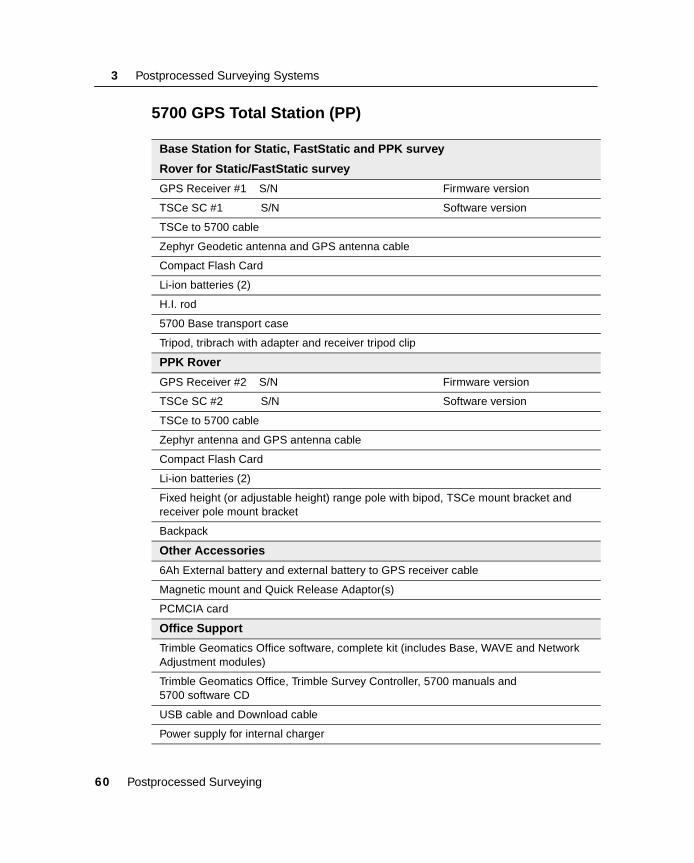
3 Postprocessed Surveying Systems
3.9.1 5700 GPS Total Station (PP)
Base Station for Static, FastStatic and PPK survey
Rover for Static/FastStatic survey
GPS Receiver #1 S/N Firmware version
TSCe SC #1 S/N Software version
TSCe to 5700 cable
Zephyr Geodetic antenna and GPS antenna cable
Compact Flash Card
Li-ion batteries (2)
H.I. rod
5700 Base transport case
Tripod, tribrach with adapter and receiver tripod clip
PPK Rover
GPS Receiver #2 S/N Firmware version
TSCe SC #2 S/N Software version
TSCe to 5700 cable
Zephyr antenna and GPS antenna cable
Compact Flash Card
Li-ion batteries (2)
Fixed height (or adjustable height) range pole with bipod, TSCe mount bracket and receiver pole mount bracket
Backpack
Other Accessories
6Ah External battery and external battery to GPS receiver cable
Magnetic mount and Quick Release Adaptor(s)
PCMCIA card
Office Support
Trimble Geomatics Office software, complete kit (includes Base, WAVE and Network Adjustment modules)
Trimble Geomatics Office, Trimble Survey Controller, 5700 manuals and5700 software CD
USB cable and Download cable
Power supply for internal charger
60 Postprocessed Surveying

Postprocessed Surveying Systems 3
3.10 Use and CareTrimble Surveying Equipment tolerates the sort of rough treatment that equipment may suffer in the field. Nevertheless, they are high-precision, electronic instruments, so treat them with reasonable care. Table 3.1 lists recommended operating parameters and conditions.
C Warning – Operating or storing your equipment outside the specified temperature range can destroy the instrument or limit its life.
Table 3.1 Recommended operating parameters for Trimble equipment
Device Temperature range Shock resistance Other
5700 receiver –40 °C to +65 °C (–40 °F to +149 °F)
1 m drop
Shock and vibration tested to 40 G random.
Waterproof to IPX7 to depth of 1 m.
Fully sealed magnesium alloy casing
TSCe –20 °C to +60 °C (–4 °F to +140 °F)
MIL-STD-810E drop. (Impact or pressure on the display screen can cause it to crack.)
Immersible in up to one meter of water, for up to one hour. Ensure that the battery compartment screws are secured tightly when replacing the battery.
Note: Removal of the backcase screws voids the warranty.
TRIMTALKTM 450S radio modem
–20 °C to +55 °C 100% fully sealed, weatherproof enclosure
TRIMMARKTM 3 radio modem
–40 °C to +65 °C (–40 °F to 149 °F)
100% fully sealed, weatherproof enclosure
Postprocessed Surveying 61

3 Postprocessed Surveying Systems
3.11 General GuidelinesTo care for your survey equipment, follow these guidelines:
• High-power signals from a nearby radio or radar transmitter can overwhelm the receiver’s circuits. This does not harm the receiver, but can prevent it from functioning. To avoid problems, try not to use the GPS receiver within 400 meters of powerful radar, television, or other transmitters. Low-power transmitters, such as the ones in portable phones and walkie-talkies, and transmission lines do not normally interfere with receiver operations.
• When plugging in a LEMO cable, make sure that the red dots on the receiver port and the cable connector line up. Never use force to plug cables in, as this may damage the pins of the connectors.
• When disconnecting a LEMO cable, use the loop provided to pull the cable connector straight out of the port. Do not turn it.
• To securely connect a TNC cable, push the connector into the port and turn it. TNC cables and the corresponding TNC ports on the 5700 receiver are color-coded to help you connect each cable to the correct port.
• Insert the 5700 internal batteries with the terminals facing the CompactFlash/USB door. Only new-generation Lithium ion batteries with a center groove can be used.
62 Postprocessed Surveying

Postprocessed Surveying Systems 3
3.12 Review Questions1. Name three data collection techniques used in PP surveys.
2. What are the requirements in terms of equipment and conditions for conducting postprocessed surveys?
3. In PPS, when and where is the integer ambiguity resolved?
4. What is the process of resolving integer ambiguities called?
5. Explain the difference between FLOAT and FIX solutions.
6. Name three initialization methods.
7. How do we know when enough data has been collected for the WAVE to compute initialization of a PPK survey?
8. List all necessary equipment (including the accessories) for Postprocessed surveying.
Postprocessed Surveying 63
3 Postprocessed Surveying Systems
3.13 Answers1. Static, FastStatic and Postprocessed Kinematic (PPK).
2. Answer:
– Two GPS receivers– Tracking carrier phase measurements– Logging data at common times and epochs– Tracking four common satellites at each station and at least
five total– Observing during good satellite geometry (DOP)– Initializing the survey (PPK)– Maintaining lock to satellites while moving (PPK)
3. During the office data processing, in WAVE module of the Trimble Geomatics Office software.
4. Initialization.
5. Answer:
– float – integer ambiguity not resolved– fix – integer ambiguity resolved, RTK system initialized
6. Known point, new point, OTF
7. TSCe SC will display PPK=FIX message in the status bar.
8. Required equipment:
– Two GPS receivers (for example, 5700 receivers) with data storage capabilities (either internal memory or a TSCe data collector)
– Two GPS antennae (for example, Zephyr or Zephyr Geodetic) and stable setups for each (for example, tripods), tape to measure the height of the tripods, or fixed-height tripods
– Postprocessing software (for example, Trimble Geomatics Office)
– Appropriate cables
64 Postprocessed Surveying

C H A P T E R
4
PPS System Components 4In this chapter:
■ Introduction
■ Session objectives
■ TSCe with Trimble Survey Controller
■ GPS receivers
■ Trimble Geomatics Office
■ Review questions
■ Answers

4 PPS System Components
4.1 IntroductionThis chapter describes the operation of the following Trimble Postprocessed system components:
• The TSCe running Trimble Survey Controller
• 5700 GPS receiver
• Trimble Geomatics Office
4.2 Session ObjectivesAt the end of this session, you will know:
• PPS system components: features and functionalities
• Trimble Survey Controller and Trimble Geomatics Office user interfaces
• How to perform basic operations
66 Postprocessed Surveying

PPS System Components 4
4.3TSCe withTrimble Survey Controller
In this section:
■ The TSCe with Trimble Survey Controller
■ Operating the TSCe data collector
■ Trimble Survey Controller sample screen displays
■ Trimble Survey Controller menu structure
■ Entering data
■ Editing data
■ Reviewing data
■ Online Help
■ Rebooting
■ Survey styles
■ Trimble GPS Survey Styles
■ Copying and editing a Survey Style
Postprocessed Surveying 67

4 PPS System Components
4.4 The TSCe with Trimble Survey Controller Postprocessed surveys can be controlled by the TSCe, running Trimble Survey Controller.
This section describes the TSCe, and shows how to use it with Trimble Survey Controller. It also gives an overview of the Trimble Survey Controller menu structure, and shows some sample TSCe screens.
The TSCe is a rugged, handheld data collector, which connects to a GPS receiver. Use the TSCe to log and enter data, transfer data to and from your office computer, and view data and information.
Trimble Survey Controller simplifies surveying by configuring and controlling receivers for GPS surveys, and by communicating with conventional instruments for conventional surveys. Trimble Survey Controller makes surveying a faster and more efficient process because it:
• stores points
• simplifies tasks
• performs numerous calculations, including coordinate geometry (Cogo) functions
• permits two-way data transfer operations
For GPS surveys, it also:
• configures the necessary receiver parameters
• monitors the receiver and survey status
A good way to learn how to use the data collector and the software is to take the TSCe into the field. Become familiar with the keypad, press various keys, look through the menus, and use the Help.
Before going into the field, make sure you have everything you need.
68 Postprocessed Surveying
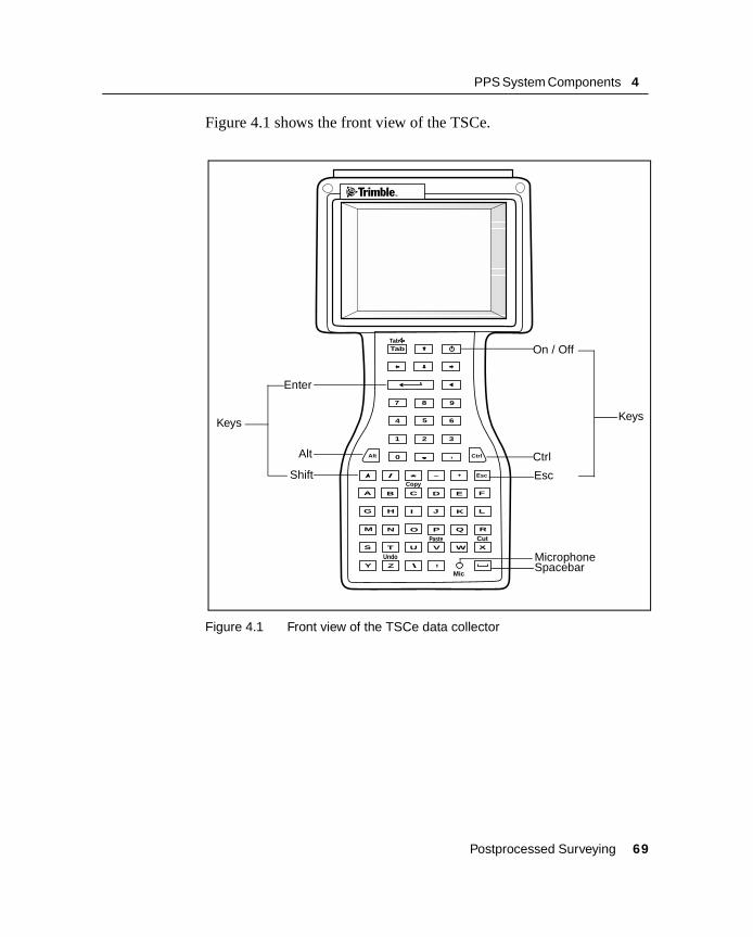
PPS System Components 4
Figure 4.1 shows the front view of the TSCe.
Figure 4.1 Front view of the TSCe data collector
Tab
Del
987
4 5 6
321
0 , Ctrl
Esc+_*/
CopyA B C D E F
G H I J
PONM
S T U V W X
K L
Q R
CutPaste
Undo
MicY Z \
Alt
Tab
Keys
Enter
Alt
Shift
Keys
On / Off
Ctrl
Esc
SpacebarMicrophone
Postprocessed Surveying 69
4 PPS System Components
4.5 Operating the TSCe Data CollectorTo turn on the TSCe, make sure the battery is inserted. Press the green | key. Hold down the same key for one second to turn it off.
4.5.1 Keys
Hard keys are the physical keys on the TSCe keypad. Examples of these are 1, 2, 3, a, b, c, =, e, , _, (, and ) . Use these keys to enter data and to access different screens.
4.5.2 Menus
Menus list Trimble Survey Controller functions. When the TSCe data collector is turned on, the Trimble logo screen appears. This is immediately followed by the main menu.
Note – To return to the main menu at any time, press the M icon.
To select a menu item select the icon by pressing the screen. Alternatively use the arrow keys to move to the required field: press the _ or * key to move up the list and press the ) or ( key to move down the list. Press \ to select the highlighted item.
4.5.3 Favorites menu
The Favorites menu provides quick access to commonly used screens (windows). You can access a screen from the Favorites list or use Q to switch between active screens.
To access a screen from the Favorites list, tap G and select the screen that you want to access.
To add a screen to the Favorites list, view the screen you want to add and select Favorites / Add to favorites. To remove a screen, view the screen and select Favorites / Remove from favorites.
70 Postprocessed Surveying

PPS System Components 4
4.5.4 Enter button
The E button performs the same action as pressing = on the TSCe keypad. The action of the E button relates to particular screens, and in some screens, the caption on the button changes to describe the action for that screen. For example, E changes to m when you are in the Measure points screen.
4.5.5 Softkeys
Softkeys (software keys) are displayed on the bottom line of the Trimble Survey Controller screen. Softkeys relate to particular screens and only appear when these screens are accessed. For example, the U softkey appears when the Antenna height field is accessed, as it relates to this field.
Tap a softkey to access it, or use the shortcut key combinations with a designated key from the keypad. For example, in the Map of current job screen, to zoom in on an area, tap N or the key combination, C+/.
Note – The # softkey appears if there are more than four softkeys associated with a screen. Tap it to see the others. Alternatively, press the ~ (Shift) key to access the other softkeys.
4.5.6 Shortcut keys
Shortcut keys (also known as access keys or hotkeys) provide a quick way of using the keypad to access menus and commonly used options. They appear as an underlined letter in the menu or option description. Hold down the A key and press the appropriate letter key to use them.
Postprocessed Surveying 71

4 PPS System Components
Table 1.2 shows the shortcut keys that are commonly used in the Trimble Survey Controller software.
Table 4.1 Trimble Survey Controller shortcut keys
Use A plus this key... to access the...
f Files menu
k Key in menu
s Survey menu
c Cogo menu
o Configuration menu
i Instrument menu
m Map of current job
e Main menu
a Favorites menu
w Switch to list
h Online Help
72 Postprocessed Surveying
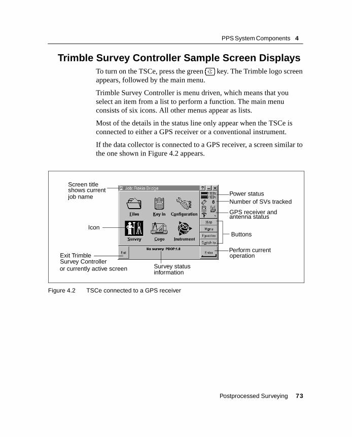
PPS System Components 4
4.6 Trimble Survey Controller Sample Screen DisplaysTo turn on the TSCe, press the green | key. The Trimble logo screen appears, followed by the main menu.
Trimble Survey Controller is menu driven, which means that you select an item from a list to perform a function. The main menu consists of six icons. All other menus appear as lists.
Most of the details in the status line only appear when the TSCe is connected to either a GPS receiver or a conventional instrument.
If the data collector is connected to a GPS receiver, a screen similar to the one shown in Figure 4.2 appears.
Figure 4.2 TSCe connected to a GPS receiver
Screen titleshows currentjob name
Icon
Exit Trimble
or currently active screenSurvey Controller
Survey statusinformation
Perform currentoperation
Power statusNumber of SVs tracked
GPS receiver and
antenna status
Buttons
Postprocessed Surveying 73
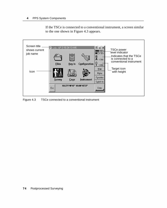
4 PPS System Components
If the TSCe is connected to a conventional instrument, a screen similar to the one shown in Figure 4.3 appears.
Figure 4.3 TSCe connected to a conventional instrument
Screen title
Icon
TSCe power
Indicates that the TSCe
shows currentlevel indicatorjob name
is connected to a
Target iconwith height
conventional instrument
74 Postprocessed Surveying
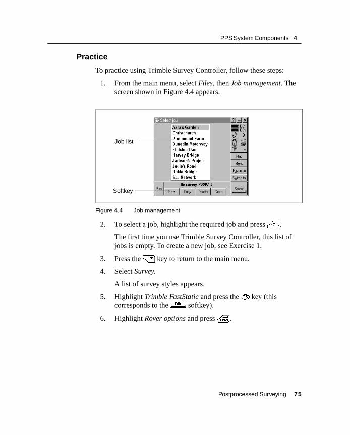
PPS System Components 4
4.6.1 Practice
To practice using Trimble Survey Controller, follow these steps:
1. From the main menu, select Files, then Job management. The screen shown in Figure 4.4 appears.
Figure 4.4 Job management
2. To select a job, highlight the required job and press \.
The first time you use Trimble Survey Controller, this list of jobs is empty. To create a new job, see Exercise 1.
3. Press the = key to return to the main menu.
4. Select Survey.
A list of survey styles appears.
5. Highlight Trimble FastStatic and press the % key (this corresponds to the f softkey).
6. Highlight Rover options and press \ .
Job list
Softkey
Postprocessed Surveying 75

4 PPS System Components
The screen shown in Figure 4.5 appears.
Figure 4.5 Rover options
7. Press = , then press the w softkey.
You return to the Survey Style menu for the chosen Style.
8. If the TSCe data collector is connected to a receiver, press \ .
The Survey menu appears.
9. Select Measure points and press \ .
If this is the first time you have used this survey style, the Style wizard prompts you to select the type of antenna and the type of radio used.
10. From the list that appears on the screen, highlight the type of antenna you are using and press \.
Arrow showsthat you chose
a listfor this field from the entry
76 Postprocessed Surveying
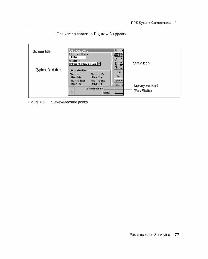
PPS System Components 4
The screen shown in Figure 4.6 appears.
Figure 4.6 Survey/Measure points
Screen title
Survey method(FastStatic)
Static icon
Typical field title
Postprocessed Surveying 77

4 PPS System Components
4.7 Trimble Survey Controller Menu StructureThe two-page Figure 4.7 gives an overview of the entire Trimble Survey Controller menu structure.
Figure 4.7 Trimble Survey Controller menu structure (continues next page)
Files
Job managementReview current jobMap of current jobStatus of current jobCopy data between jobsImport / ExportWindows Explorer
Key in
PointsLinesArcs
Survey – Items depend on the type of survey you are doing
Start base receiverStation setupStart surveyStart/Stop PP infillMeasure points
Points
Send ASCII dataReceive ASCII data
RoadsTemplatesNotes
Boundary
End surveySwap base receiverSite calibrationInitializationStakeout...Measure laser pointsOffsetsContinuous topoMeasure rounds
Comma separated files
LinesArcsDTMsRoads
78 Postprocessed Surveying

PPS System Components 4
Keep this figure handy as a reference until you are familiar with the menu structure.
Job...Controller...Feature & attribute librariesSurvey Styles...
Coordinate systemUnitsCogo settings
Time/date
Rover options
Cogo
Compute inverseCompute intersectionsCompute areaCompute azimuthCompute distanceSubdivide a lineSubdivide an arcTraverse
Instrument
SatellitesReceiver filesPositionReceiver statusOptions
Configuration
Items depend on the typeof instrument the TSCe datacollector is connected to
Items depend on theSurvey Style selected
Navigate to pointStation setup detailsTarget detailsInstrument controls
LanguageSound events
Topo pointRover radioBase optionsBase radioLaser rangefinderFastStatic pointObserved control pointRapid pointContinuous pointsStakeoutInstrumentTargetRoundsSite calibrationPP initialization timesDuplicate point actionsCorrectionsTraverse options
Postprocessed Surveying 79
4 PPS System Components
4.8 Entering DataData must be entered before Trimble Survey Controller can perform most of its functions. A typical screen has several fields into which you can enter data. For some fields you select an option from a list, while for others you key in alphanumeric details.
4.8.1 Choosing an Option
For some fields, you select a parameter setting from a list of options. These fields have a ) symbol on the left (see the sample Rover options screen on page 76).
There are two ways to select an option:
• Use the touch screen to select the options required
• Use the arrow keys to select your options and \ to store the option
4.8.2 Keying in Data
To enter data, highlight the field by touching the screen or using the arrow keys. This takes you to the beginning of the field. Key in the details. When the details are complete, press \ or the enter icon on the screen. Press \ again to accept the screen.
80 Postprocessed Surveying

PPS System Components 4
4.9 Editing DataTo edit details in a field, highlight the field by clicking or double clicking on the screen where you want to edit. Alternatively you can use the arrow keys to move to the field you wish to edit.
4.10 Reviewing DataYou can review the data in the Trimble Survey Controller database at any time.
To review data, select Files from the main menu. Then select Review current job.
Records are stored in chronological order. The last (most recent) page of the database appears first when you access the database.
Press the p and P softkeys to move up and down in the database one page at a time. Press the _ and ) keys to move up and down one record at a time.
Use the æ softkey to find records elsewhere in the database. For example, it is possible to search for points surveyed several hours ago. To access the Search menu, press æ. Select a type of search. You can choose to repeat a previous search, or to search by name, code, or current record type.
For more information about a record, highlight it and double click on the screen or press \ . To return to the database list, press = .
You can edit some fields, such as Code and Antenna height.
Note – If point coordinates appear as ‘?’, see the Note on the next page.
Postprocessed Surveying 81

4 PPS System Components
4.10.1 Coordinate View Setting
The setting in the Coordinate view field (WGS-84, Local, Grid, or HA VA SD, for example) determines which values appear in the point record. You can change the coordinate view setting for an entire job, or just when viewing a point.
To change the Coordinate view setting for a point that you want to view:
1. When reviewing the database, highlight the point record and press \ .
2. Press o and set the Coordinate view field as required.
Note – If no datum transformation and no projection are defined and the Coordinate view field is set to Local or Grid, the coordinate values for GPS points will be ‘?’. Change the Coordinate view setting to WGS-84.
4.11 Online HelpOnline help for the Trimble Survey Controller software is displayed in Hyper-text Markup Language (HTML) pages. You can click on any underlined text (link) to move to the page it describes.
There are several ways to obtain help while you are using the Trimble Survey Controller software:
• To access help within the Trimble Survey Controller software, tap 4 or press A+h.
An index of all the topics appears, with the default topic for the current screen highlighted. Do one of the following:
– To view this topic, tap the topic.
– To search for a different topic, enter a new keyword or scroll through the list.
82 Postprocessed Surveying
PPS System Components 4
B Tip – To move quickly to a Help topic, type the first few letters of the topic. Then use the arrow keys if necessary.
4.12 RebootingIf the TSCe does not respond to keystrokes, check that the TSCe is receiving power. If power is uninhibited, you may need to reboot.
To reboot, turn the TSCe off and then on again.
If the TSCe data collector fails to respond to keystrokes, you may need to reboot the system. Turn off the data collector and turn it back on again.
If this does not work then perform a soft reset.
Soft reset
A soft reset (warm boot) shuts down the hardware and restarts the Trimble Survey Controller software. You will not lose any data by performing a warm boot.
To perform a soft reset:
• Hold down ~ and C, while you press and release _.
The TSCe data collector will reset to the default Microsoft Windows desktop view.
Hard reset
You will not lose any data that is stored on the built-in storage card (the \Disk folder) by performing a hard reset (cold boot). The contents of the RAM memory will be cleared, including any desktop shortcuts that you have created.
Postprocessed Surveying 83

4 PPS System Components
To perform a hard reset:
1. Hold down _.
After approximately 5 seconds, a dialog and a countdown timer appear, indicating that the TSCe data collector will reset.
2. Continue to hold _ for 5 seconds, then release.
The TSCe data collector will briefly display the boot screen and then reset to the default Microsoft Windows desktop view.
84 Postprocessed Surveying

PPS System Components 4
4.13 Survey StylesThere are two kinds of survey style: GPS and Conventional. They appear together in the Select Survey Style list.
When using Trimble Survey Controller for a GPS survey, choose from one of nine survey types. These types are based on the kinematic, differential, and FastStatic techniques. To select the survey type you need, select an appropriate survey style.
4.13.1 The Concept of Survey Styles
Survey Styles make Trimble Survey Controller easier to use. Use them to change the configuration of Trimble Survey Controller quickly and easily for different types of survey.
In a GPS survey, the survey style instructs the base and rover receivers to perform the functions required for a specific survey type. It also defines the parameters for measuring and storing points. This whole set of information is stored as a template that can be called up and reused when necessary.
A GPS survey style defines the survey type, antenna information, elevation mask, PDOP mask, and point occupation times. If applicable, it also defines the following:
• Logging intervals
• Initialization times
• Site calibration defaults
• GPS file storage location
• Real-time broadcast message format
• Radio communication parameters
Postprocessed Surveying 85
4 PPS System Components
4.13.2 Choosing a Survey Style
Trimble provides four GPS survey styles that cover four of the nine possible survey types. To use any survey type not covered by the Trimble survey styles, you must create your own survey style. This is described in Exercise 2.
4.14 Trimble GPS Survey StylesThe four standard Trimble GPS survey styles supplied with the Trimble Survey Controller system are:
• RTK
• RTK & Infill
• PPK
• FastStatic
These styles cover the four most popular centimeter-level survey types. To use the default settings for a survey type, select the appropriate style and use it as it is.
You cannot delete a Trimble survey style, but you can copy one and edit some of the fields in the copy that you make.
Note – This training manual addresses Trimble FastStatic and Trimble Trimble PP Kinematic Styles only.
4.14.1 Trimble FastStatic Survey Style
The Trimble FastStatic survey style prepares the Trimble Survey Controller software for a Static or FastStatic survey.
Use this Style for control surveys when no radio is available.
By default, the base receiver is instructed to log raw data atfive-second intervals for the duration of the survey.
86 Postprocessed Surveying

PPS System Components 4
4.14.2 Trimble PP Kinematic Survey Style
The Trimble PP Kinematic survey style prepares the Trimble Survey Controller software for a Postprocessed Kinematic survey. No radio is required for a PPK survey.
Use this style for topographic or control surveys when no radio is available.
By default, the base receiver is instructed to log raw data at five second intervals for the duration of the survey.
Default settings
The default elevation mask for the base receiver and the rover receiver is 13°. The default PDOP mask setting is 6. Other default settings define how point measurements are made.
Note – When editing an option, you cannot access every field in the screen that appears. For example, the setting in the Survey type field is fixed for each Trimble survey style.
Postprocessed Surveying 87
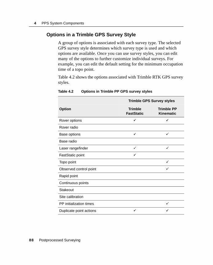
4 PPS System Components
4.14.3 Options in a Trimble GPS Survey Style
A group of options is associated with each survey type. The selected GPS survey style determines which survey type is used and which options are available. Once you can use survey styles, you can edit many of the options to further customize individual surveys. For example, you can edit the default setting for the minimum occupation time of a topo point.
Table 4.2 shows the options associated with Trimble RTK GPS survey styles.
Table 4.2 Options in Trimble PP GPS survey styles
Trimble GPS Survey styles
Option Trimble FastStatic
Trimble PP Kinematic
Rover options � �
Rover radio
Base options � �
Base radio
Laser rangefinder � �
FastStatic point �
Topo point �
Observed control point �
Rapid point
Continuous points
Stakeout
Site calibration
PP initialization times �
Duplicate point actions � �
88 Postprocessed Surveying

PPS System Components 4
Exercise 1: Create a New Job
To create a job:
1. Turn on the TSCe data collector.
2. From the main menu, select Files.
3. Select Job management then press the n softkey.
4. Type the job name. Press \ to accept the job name.
5. The Select coordinate system screen appears. Do one of the following:
– Select a system from the list.To do this, choose Select from library and select a system from the list. Select the zone for the system. Set the Use geoid model field to No.
– Key in the datum transformation and projection parameters for the site.To do this, select Key in parameters then Datum transformation and enter the details for the site. Press \ then select Projection and enter the details. Press \ again to accept the details.
– Copy a coordinate system from another job in the database.To do this, select Copy from other job and select the job name to copy from.
– Select no projection and no datum transformation.To do this, select No projection/no datum.
Set the Coordinates field to Ground and enter a value in the Reference elevation field. Alternatively, set the Coordinate field to Grid.
Set the Use geoid model field to Yes and select a geoid model to calculate a Geoid/Inclined plane vertical adjustment after a site calibration.
Postprocessed Surveying 89
4 PPS System Components
For a survey where GPS measurements are to be combined with conventional observations later, choose a coordinate system now. For more information, refer to the Trimble Survey Controller Reference Manual.
Note – If you are not sure of the coordinate system, select No projection/no datum. Set the Coordinates field to Ground and enter the average site elevation in the Reference elevation field. Define these parameters later in the job and all points will be updated. (To do this, select Configuration / Job / Coordinate system. Press the k or * softkey and enter the parameters or select a coordinate system.)
If no datum transformation and no projection are defined, any points measured using GPS are only displayed as WGS-84 coordinates. Any points measured using a conventional instrument are displayed with null (?) coordinates.
6. After selecting or keying in a coordinate system, press the w softkey.
The job is created.
90 Postprocessed Surveying

PPS System Components 4
Exercise 2: Create a PP Kinematic Survey Style
Trimble Survey Controller provides Trimble survey styles that configure the hardware for four of the seven possible GPS survey types—RTK, RTK & infill, FastStatic, and PP Kinematic.
The other available survey types are:
• RTK & data logging
• RT differential
• RT diff & data logging
To survey using any of these types a new survey style has to be created. Existing Survey Styles can also be edited
To do this:
1. From the main menu, select Configuration/Survey Styles.
2. Press n .
3. Enter a name in the Style name field and press \ .
4. In the Style type field choose GPS.
5. Press \ .
Note – When you create a new GPS survey style, it is configured as an RTK survey that you must edit.
Postprocessed Surveying 91
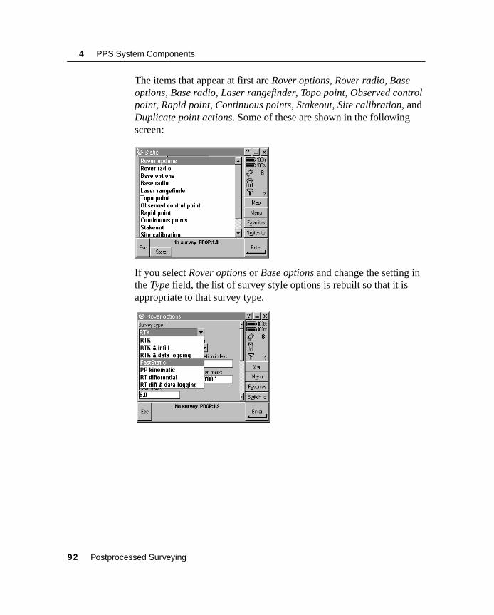
4 PPS System Components
The items that appear at first are Rover options, Rover radio, Base options, Base radio, Laser rangefinder, Topo point, Observed control point, Rapid point, Continuous points, Stakeout, Site calibration, and Duplicate point actions. Some of these are shown in the following screen:
If you select Rover options or Base options and change the setting in the Type field, the list of survey style options is rebuilt so that it is appropriate to that survey type.
92 Postprocessed Surveying
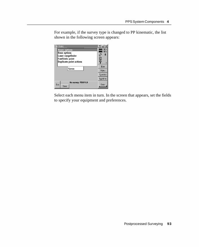
PPS System Components 4
For example, if the survey type is changed to PP kinematic, the list shown in the following screen appears:
Select each menu item in turn. In the screen that appears, set the fields to specify your equipment and preferences.
Postprocessed Surveying 93
4 PPS System Components
4.15 Editing a Survey StyleEdit a survey style to define new field observation procedures or to set options for new hardware, such as radios and receivers.
Trimble survey styles can be edited, but the survey type (RTK, RTK & infill, PP Kinematic, and FastStatic) is fixed and cannot be changed.
Any survey style that you create by copying an original or edited Trimble survey style is also locked in this way. If you create your own survey styles, however, you can copy and edit them without limitation.
To edit a survey style:
1. End the current survey.
2. From the main menu select Configuration/Survey Styles. The list of survey styles appears. Highlight the name of the Style to be edited and press f. The list of options for that survey style appears.
3. Change the settings in each option as required.
94 Postprocessed Surveying
PPS System Components 4
4.16GPS Receivers
In this section:
■ The Trimble 5700 GPS receiver
■ Data management
Postprocessed Surveying 95

4 PPS System Components
96 Postprocessed Surveying

PPS System Components 4
4.17 The Trimble 5700 GPS Receiver All the controls that you need for Static/FastStatic general operation of the 5700 receiver are located on the front panel.
For PPK surveys, the 5700 receiver uses a Trimble Survey Controller as an interface. The 5700 receiver can be configured as an autonomous base station or roving receiver.
Figure 4.8 5700 receiver front panel
4.17.1 Button Functions
The 5700 receiver has only two buttons: a power button, represented in this manual by p; and a data button, represented by d.
Use p to switch the receiver on or off, and to perform data management functions such as deleting files or resetting the receiver.
2 3
t
Logging/Memory LED
Data button Power button
Battery LEDsSV Tracking
Radio/Event
LED
Marker LED
Postprocessed Surveying 97

4 PPS System Components
Use d to start or stop logging. This button is only effective when the receiver is switched on and has completed any power-up and initialization tasks.
Table 4.3 describes the main functions of the two buttons.
Note – The term “press” indicates that you should press the button down and release it immediately. The term “hold” indicates that you should press the button down and hold it down until the time indicated has elapsed.
Table 4.3 Button functions
Action Power button Data button
Turn the receiver on Press
Turn the receiver off Hold for 2 seconds
Start logging data internally Press
Stop logging data internally Hold for 2 seconds
Delete the ephemeris file Hold for 15 seconds
Reset the receiver to factory defaults Hold for 15 seconds
Delete application files Hold for 30 seconds
Format the CompactFlash card Hold for 30 seconds
98 Postprocessed Surveying
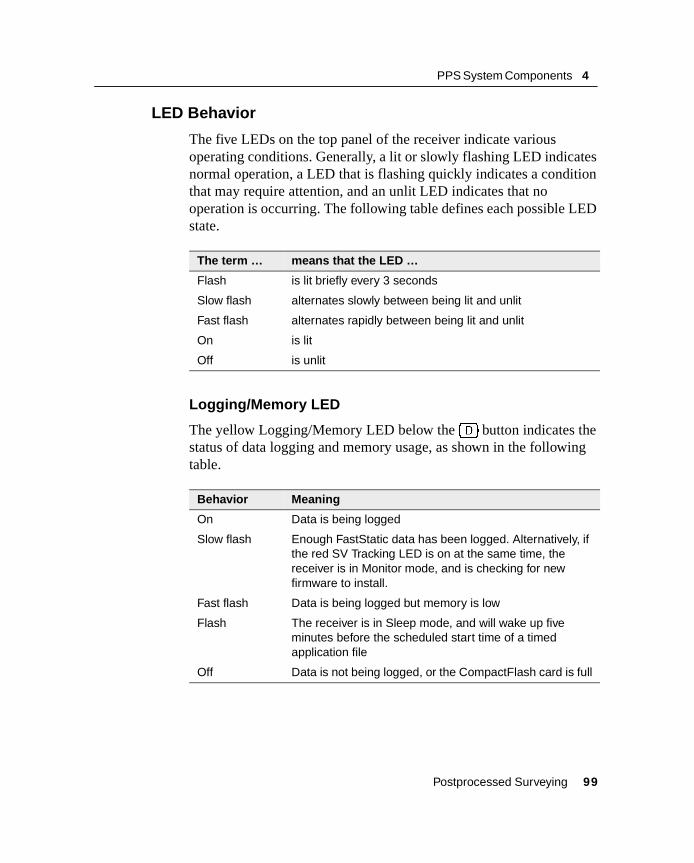
PPS System Components 4
4.17.2 LED Behavior
The five LEDs on the top panel of the receiver indicate various operating conditions. Generally, a lit or slowly flashing LED indicates normal operation, a LED that is flashing quickly indicates a condition that may require attention, and an unlit LED indicates that no operation is occurring. The following table defines each possible LED state.
Logging/Memory LED
The yellow Logging/Memory LED below the d button indicates the status of data logging and memory usage, as shown in the following table.
The term … means that the LED …
Flash is lit briefly every 3 seconds
Slow flash alternates slowly between being lit and unlit
Fast flash alternates rapidly between being lit and unlit
On is lit
Off is unlit
Behavior Meaning
On Data is being logged
Slow flash Enough FastStatic data has been logged. Alternatively, if the red SV Tracking LED is on at the same time, the receiver is in Monitor mode, and is checking for new firmware to install.
Fast flash Data is being logged but memory is low
Flash The receiver is in Sleep mode, and will wake up five minutes before the scheduled start time of a timed application file
Off Data is not being logged, or the CompactFlash card is full
Postprocessed Surveying 99
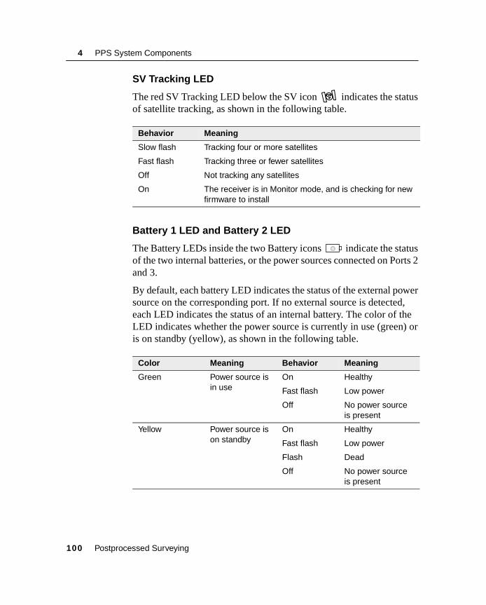
4 PPS System Components
SV Tracking LED
The red SV Tracking LED below the SV icon indicates the status of satellite tracking, as shown in the following table.
Battery 1 LED and Battery 2 LED
The Battery LEDs inside the two Battery icons indicate the status of the two internal batteries, or the power sources connected on Ports 2 and 3.
By default, each battery LED indicates the status of the external power source on the corresponding port. If no external source is detected, each LED indicates the status of an internal battery. The color of the LED indicates whether the power source is currently in use (green) or is on standby (yellow), as shown in the following table.
Behavior Meaning
Slow flash Tracking four or more satellites
Fast flash Tracking three or fewer satellites
Off Not tracking any satellites
On The receiver is in Monitor mode, and is checking for new firmware to install
Color Meaning Behavior Meaning
Green Power source is in use
On Healthy
Fast flash Low power
Off No power source is present
Yellow Power source is on standby
On Healthy
Fast flash Low power
Flash Dead
Off No power source is present
100 Postprocessed Surveying

PPS System Components 4
Radio LED
The green Radio LED below the Radio icon indicates the status of data input and output. Slow flash indicates that an information packet or event marker has been received.
4.17.3 Communication Ports
Figure 4.9 shows the ports on the 5700 receiver.
Figure 4.9 5700 receiver ports
Table 4.4 shows the icons available on the 5700 ports:
Table 4.4 5700 receiver ports
Icon Name Connections
Port 1 TSCe data collector, event marker, or computer
Port 2 Power in, computer, 1PPS, or event marker
1 2
GPS RADIO
USB port
CompactFlash cardGPS antenna Radio antennaGPS antenna
Postprocessed Surveying 101

4 PPS System Components
4.17.4 Starting and Stopping the Receiver
To turn on the receiver, press p.
To turn off the receiver, hold down p for two seconds.
In RTK surveys, starting and stopping the receiver is controlled by Trimble Survey Controller.
4.17.5 Logging Data
You can log data on the 5700 receiver, or you can use the receiver to generate GPS data, which is logged to a TSCe.
Logging to Trimble Survey Controller
When the 5700 receiver is connected to a data collector running Trimble Survey Controller, you can log GPS data from the receiver to the data collector, or to a PC card inserted in the data collector. When you use Trimble Survey Controller, you do not use the receiver’s controls. Instead, you use Trimble Survey Controller functions to set logging options, specify filenames, and control when logging occurs.
Data is stored in job files, which can be transferred to your office computer using Trimble’s Data Transfer utility.
Port 3 External radio, power in
ANT GPS antenna
RADIO Radio communications antenna
Table 4.4 5700 receiver ports (Continued)
Icon Name Connections
102 Postprocessed Surveying
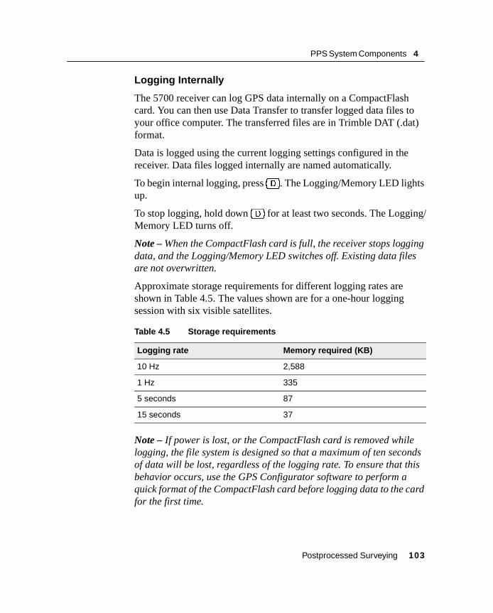
PPS System Components 4
Logging Internally
The 5700 receiver can log GPS data internally on a CompactFlash card. You can then use Data Transfer to transfer logged data files to your office computer. The transferred files are in Trimble DAT (.dat) format.
Data is logged using the current logging settings configured in the receiver. Data files logged internally are named automatically.
To begin internal logging, press d. The Logging/Memory LED lights up.
To stop logging, hold down d for at least two seconds. The Logging/Memory LED turns off.
Note – When the CompactFlash card is full, the receiver stops logging data, and the Logging/Memory LED switches off. Existing data files are not overwritten.
Approximate storage requirements for different logging rates are shown in Table 4.5. The values shown are for a one-hour logging session with six visible satellites.
Note – If power is lost, or the CompactFlash card is removed while logging, the file system is designed so that a maximum of ten seconds of data will be lost, regardless of the logging rate. To ensure that this behavior occurs, use the GPS Configurator software to perform a quick format of the CompactFlash card before logging data to the card for the first time.
Table 4.5 Storage requirements
Logging rate Memory required (KB)
10 Hz 2,588
1 Hz 335
5 seconds 87
15 seconds 37
Postprocessed Surveying 103
4 PPS System Components
4.17.6 Resetting to Defaults
To reset the 5700 receiver to its factory default settings, hold down p for at least 15 seconds.
C Warning – Do not hold down p for more than 30 seconds. After 30 seconds, any application files stored in the receiver are deleted and the CompactFlash card is reformatted.
Resetting the receiver to its factory defaults also deletes any ephemeris file in the receiver.
4.17.7 Formatting a CompactFlash Card
To format a CompactFlash card for use in a 5700 receiver, insert the card in the CompactFlash port, then hold down p for at least 30 seconds. After 15 seconds, the receiver is reset to its factory defaults, and any ephemeris file is deleted. After 30 seconds, any files stored on the card are deleted and the CompactFlash card is reformatted.
C Warning – Formatting a CompactFlash card while it is in the receiver deletes all the data files on the card and all the application files in the receiver.
Note – When you use p to format the CompactFlash card, a quick format is performed. A quick format reformats the card for use with the 5700 receiver and deletes all data on the card. A full format also checks the card for errors and bad sectors. A full format is only necessary if the card is corrupted. To perform a full format, use the GPS Configurator software.
104 Postprocessed Surveying
PPS System Components 4
4.17.8 Firmware
A receiver’s firmware is the program inside the receiver that makes the receiver run and controls the hardware. You can upgrade the firmware for the 5700 receiver in either of the following ways:
• Using the WinFLASH software
• Copying the firmware (.elf) file directly to the CompactFlash card
Trimble recommends that you use the WinFLASH software to upgrade the firmware.
To upgrade the receiver firmware by copying the .elf file to the CompactFlash card:
1. Connect the CompactFlash card to your desktop computer.
2. Using Microsoft Windows Explorer, copy the .elf file from your computer to the CompactFlash card.
3. Disconnect the CompactFlash card from your computer and insert it into the receiver.
4. Turn the receiver off.
5. Hold down d and press p.
The receiver starts in Monitor mode, automatically detects the newer version of the firmware, and installs it. In Monitor mode, the red SV Tracking LED is lit and the yellow Logging/Memory LED flashes slowly.
The upgrade takes about two minutes. Once the upgrade procedure is complete, the receiver restarts automatically.
C Warning – Upgrading the firmware deletes all application files on the 5700 receiver.
Postprocessed Surveying 105

4 PPS System Components
4.18 Data ManagementThe 5700 receiver automatically assigns a filename and creates a tracking session file when Data button is pressed and the receiver is tracking four or more satellites after start-up.
Each filename identifies the specific receiver by serial number, lists the GPS date, and file sequence number as follows: AAAABBBC
Where:
AAAA = the last four digits of the receiver serial number
BBB = GPS date code (Julian day, where: Jan 1 = 001, Dec 31 = 365)
C = session sequence number (0–9, A–Z)
This numbering scheme allows up to 42 session files to be uniquely
numbered.
The GPS receiver stops recording data when the internal memory is full or if 42 sessions have been recorded.
To check when the receiver internal data memory is almost full or has become full, check the data logging LED behavior.
For more information on GPS receiver default operating parameters, see Appendix A, Configuration.
Note – The 5700 GPS receiver operating parameters for Static and FastStatic surveys can be configured using the GPS Configurator or the Configuration Toolbox utilities.
106 Postprocessed Surveying

PPS System Components 4
4.19Trimble Geomatics Office
In this section:
■ Starting Trimble Geomatics Office
■ The Trimble Geomatics Office window
■ The Survey view
■ Other modules
■ The Plan view
■ Properties window overview
■ Viewing survey data in the Properties window
■ Viewing and editing points
■ Viewing observations
■ Changing the project properties
■ Using project templates
■ Trimble Data Transfer utility
■ Managing your devices
■ Review questions
■ Answers
Postprocessed Surveying 107

4 PPS System Components
108 Postprocessed Surveying
PPS System Components 4
4.20 Starting Trimble Geomatics OfficeTo start the software:
• Click and then select Programs / Trimble Geomatics Office / Trimble Geomatics Office.
The Trimble Geomatics Office window appears.
4.21 The Trimble Geomatics Office WindowThe Trimble Geomatics Office window includes the main graphics window (which displays project data), menus, and toolbars.
There are two views—Survey and Plan. In each view the available menus, menu commands, and toolbars are different.
To switch between the Survey and Plan views, do one of the following:
• In the toolbar, select the Survey View tool or the Plan View tool.
• Select View / Survey or View / Plan.
Postprocessed Surveying 109

4 PPS System Components
Figure 4.10 shows the parts of the Trimble Geomatics Office window that are common to both views.
Figure 4.10 Parts of the graphics window common to both views
Project Menucommands
Projectname
Graphicswindow
Toolbars Systembuttons
bar
Zoom navigatorwindow
Statusbar
Windowcorner
110 Postprocessed Surveying
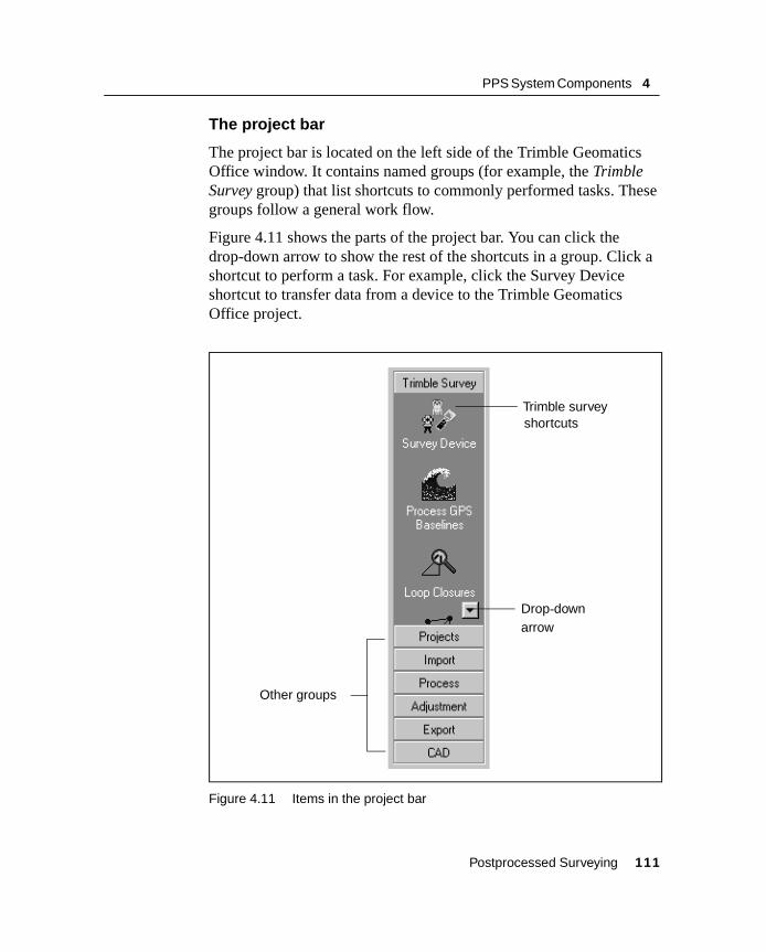
PPS System Components 4
The project bar
The project bar is located on the left side of the Trimble Geomatics Office window. It contains named groups (for example, the Trimble Survey group) that list shortcuts to commonly performed tasks. These groups follow a general work flow.
Figure 4.11 shows the parts of the project bar. You can click the drop-down arrow to show the rest of the shortcuts in a group. Click a shortcut to perform a task. For example, click the Survey Device shortcut to transfer data from a device to the Trimble Geomatics Office project.
Figure 4.11 Items in the project bar
Trimble surveyshortcuts
Drop-downarrow
Other groups
Postprocessed Surveying 111

4 PPS System Components
To show or hide the project bar, do one of the following:
• In the toolbar, click the Project Bar icon.
• Select View / Project Bar.
When there is no project open, the Projects and Utilities groups are available. When a project is open, only the Utilities group is unavailable.
The zoom navigator
The zoom navigator is a small window located at the bottom of the project bar. It reflects the data displayed in the main Trimble Geomatics Office graphics window. If you use any of the zoom tools in the main window, the zoom navigator changes to reflect this. It is a convenient display of the extents of your project.
You can show or hide the zoom navigator within the project bar. To do this:
• In the project bar, right-click to access the shortcut menu and then select Zoom Navigator.
To use the zoom navigator:
• Click an area of the project in the zoom navigator. This area becomes the center of the main graphics window.
To use the zoom navigator to zoom:
• In the zoom navigator, drag a box around the area of interest. The main graphics window displays the same data.
When you point to the middle of the box in the zoom navigator, the pointer becomes a . This means that you can drag the box over the project area without changing the zoom. The view of the project in the main graphics window reflects these movements.
B Tip – If you have a mouse with a wheel, you can use the wheel to change the size of the zoom navigator box.
112 Postprocessed Surveying
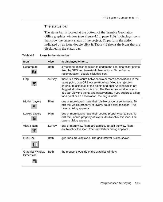
PPS System Components 4
The status bar
The status bar is located at the bottom of the Trimble Geomatics Office graphics window (see Figure 4.10, page 110). It displays icons that show the current status of the project. To perform the action indicated by an icon, double-click it. Table 4.6 shows the icons that are displayed in the status bar.
Table 4.6 Icons in the status bar
Icon View Is displayed when...
Recompute Both a recomputation is required to update the coordinates for points fixed by GPS and terrestrial observations. To perform a recomputation, double-click this icon.
Flag Survey there is a misclosure between two or more observations to the same point, or a GPS observation has failed the rejection criteria. To select all of the points and observations which are flagged, double-click this icon. The Properties window opens. You can view the points and observations. If you suppress a flag for a point or an observation, the flag is white.
Hidden Layers Plan one or more layers have their Visible property set to false. To edit the Visible property of layers, double-click this icon. The Layers dialog appears.
Locked Layers Plan one or more layers have their Locked property set to true. To edit the Locked property of layers, double-click this icon. The Layers dialog appears.
View Filters Survey one or more view filters are applied. To edit the view filters, double-click this icon. The View Filters dialog appears.
Grid Line Both grid lines are displayed. The grid interval is also shown.
Graphics Window Dimension
Both the mouse is outside of the graphics window.
Postprocessed Surveying 113

4 PPS System Components
4.22 The Survey ViewIn the Survey view, GPS and terrestrial observations are displayed as colored lines. Control points and network adjusted points also have special displays.
If Trimble Geomatics Office finds any problematic observations (for example, a misclosure outside the tolerance specified in the Horizontal or Vertical fields of the Recompute tab in the Project Properties dialog), error flags appear at the point where the misclosure occurs. Use the Survey view to perform survey-related tasks such as:
• checking GPS and conventional observations
• correcting erroneous data
• GPS processing (if you have the WAVE Baseline Processing module installed)
• GPS site calibration
• GPS loop closures
• inverse calculations
• Network Adjustment (if you have the Network Adjustment module installed)
For more information, refer to the Trimble Geomatics Office Help.
114 Postprocessed Surveying
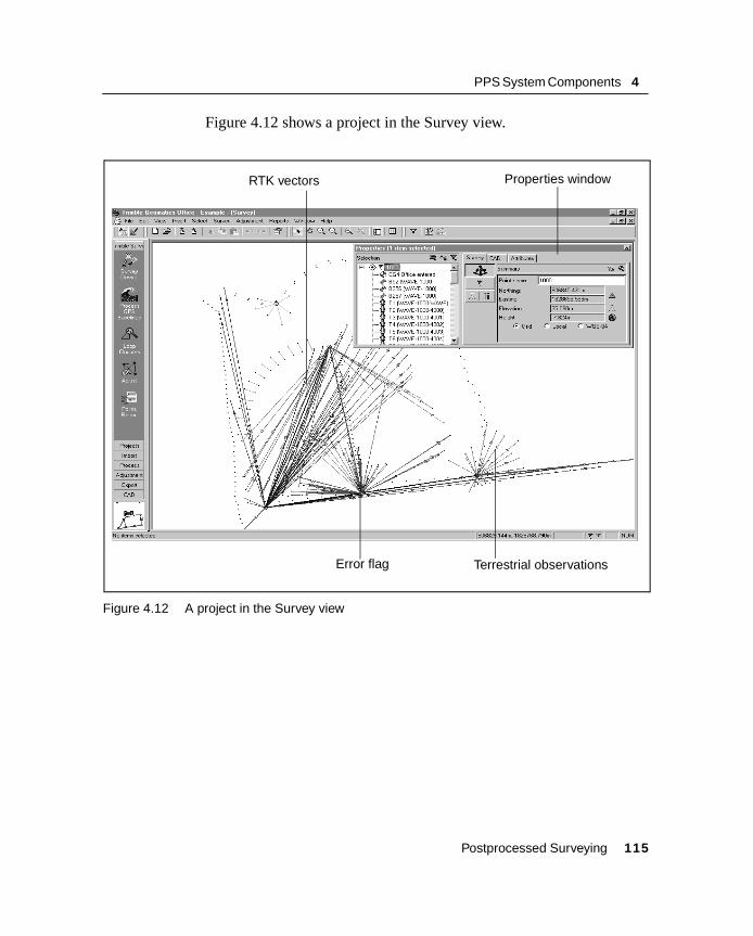
PPS System Components 4
Figure 4.12 shows a project in the Survey view.
Figure 4.12 A project in the Survey view
RTK vectors Properties window
Error flag Terrestrial observations
Postprocessed Surveying 115
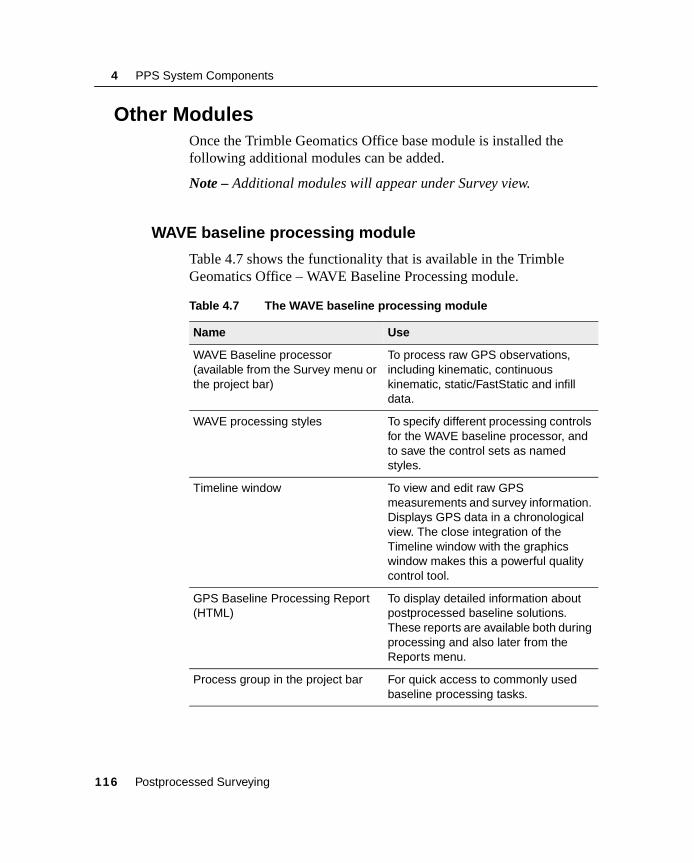
4 PPS System Components
4.23 Other ModulesOnce the Trimble Geomatics Office base module is installed the following additional modules can be added.
Note – Additional modules will appear under Survey view.
4.23.1 WAVE baseline processing module
Table 4.7 shows the functionality that is available in the Trimble Geomatics Office – WAVE Baseline Processing module.
Table 4.7 The WAVE baseline processing module
Name Use
WAVE Baseline processor (available from the Survey menu or the project bar)
To process raw GPS observations, including kinematic, continuous kinematic, static/FastStatic and infill data.
WAVE processing styles To specify different processing controls for the WAVE baseline processor, and to save the control sets as named styles.
Timeline window To view and edit raw GPS measurements and survey information. Displays GPS data in a chronological view. The close integration of the Timeline window with the graphics window makes this a powerful quality control tool.
GPS Baseline Processing Report (HTML)
To display detailed information about postprocessed baseline solutions. These reports are available both during processing and also later from the Reports menu.
Process group in the project bar For quick access to commonly used baseline processing tasks.
116 Postprocessed Surveying

PPS System Components 4
4.23.2 Network adjustment module
Table 4.8 shows the functionality that is available in the Trimble Geomatics Office – Network Adjustment module.
Note – For RTK surveys, only base module is required.
For RTK & Infill surveys, WAVE module is required for processing Infill data.
If you wish to include RTK baselines into a network adjustment, the Network Adjustment module is required. Make sure QC2 records are collected in the field.
Table 4.8 The Network adjustment module
Name Use
Network Adjustment (available from the Adjustment menu or the project bar).
Allowing you to fix points, load observations for Network Adjustment, determine observation outliers, and weight the observation errors.
To adjust your GPS and terrestrial networks, analyze the results, edit the network parameters, and readjust.
Network Adjustment styles To specify different adjustment controls for the Network Adjustment software, and to save the control sets as named styles.
Network Adjustment Report (HTML)
To review the results of the adjustment and perform quality control checks.
Adjustment group in project bar
For quick access to commonly-used network adjustment processing tasks.
Ellipse Controls toolbar To configure the appearance of error ellipses in the graphics window after a network adjustment.
Postprocessed Surveying 117
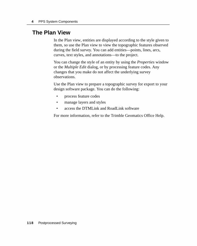
4 PPS System Components
4.24 The Plan ViewIn the Plan view, entities are displayed according to the style given to them, so use the Plan view to view the topographic features observed during the field survey. You can add entities—points, lines, arcs, curves, text styles, and annotations—to the project.
You can change the style of an entity by using the Properties window or the Multiple Edit dialog, or by processing feature codes. Any changes that you make do not affect the underlying survey observations.
Use the Plan view to prepare a topographic survey for export to your design software package. You can do the following:
• process feature codes
• manage layers and styles
• access the DTMLink and RoadLink software
For more information, refer to the Trimble Geomatics Office Help.
118 Postprocessed Surveying
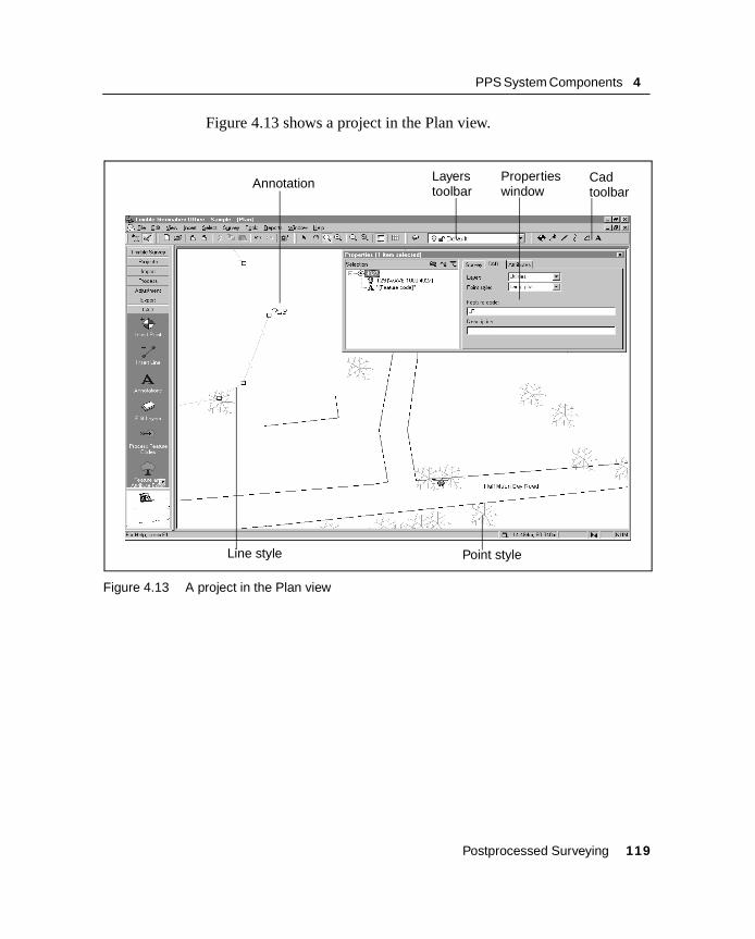
PPS System Components 4
Figure 4.13 shows a project in the Plan view.
Figure 4.13 A project in the Plan view
Properties window
Annotation Layerstoolbar
Cadtoolbar
Line style Point style
Postprocessed Surveying 119

4 PPS System Components
4.24.1 ToolTips
ToolTips are a quick way to learn about, or recall the function of, a button, box, or tool. They also provide useful information about entities in the graphics window. To use ToolTips:
• Position the pointer over a button, box, or tool in the toolbar; or an entity (observation, point, line, arc, curve, text, or annotation) in the graphics window.
After a few seconds, a small pop-up window appears and identifies the item. This is a ToolTip.
For example, when you position the pointer over the Import tool in the standard toolbar, the following ToolTip appears:
For more information about what each tool does, refer to the Help.
4.24.2 Shortcut Menus
Shortcut menus are context-sensitive menus with commands that vary depending on where you position the pointer.
You can use shortcut menus for common tasks such as:
• accessing commonly-used menu commands and dialogs
• toggling display settings
• inserting field codes
To access a shortcut menu:
1. In the appropriate area, click the right mouse button (right-click). A shortcut menu appears.
2. Select the appropriate menu command.
120 Postprocessed Surveying
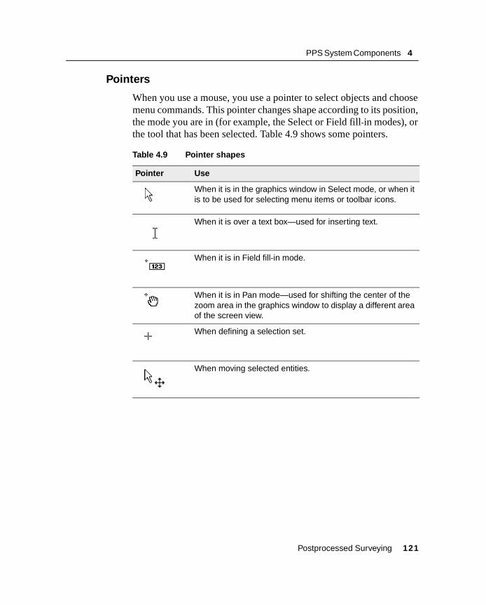
PPS System Components 4
4.24.3 Pointers
When you use a mouse, you use a pointer to select objects and choose menu commands. This pointer changes shape according to its position, the mode you are in (for example, the Select or Field fill-in modes), or the tool that has been selected. Table 4.9 shows some pointers.
Table 4.9 Pointer shapes
Pointer Use
When it is in the graphics window in Select mode, or when it is to be used for selecting menu items or toolbar icons.
When it is over a text box—used for inserting text.
When it is in Field fill-in mode.
When it is in Pan mode—used for shifting the center of the zoom area in the graphics window to display a different area of the screen view.
When defining a selection set.
When moving selected entities.
Postprocessed Surveying 121

4 PPS System Components
4.24.4 Color and Symbol Schemes
Table 4.10 shows the available colors and symbols.
Table 4.10 Colors and symbols
Item Default legend Black legend
Default color for text Window text color in Control Panel
White
Trimble Geomatics Office graphics window
Window color in Control Panel
Black
Color of selected entities Selected items color in Control Panel
Red
More than one type of observation (for example a terrestrial and an RTK observation between two points)
Black White
RTK vectors Blue Blue
Postprocessed static baselines Orange Yellow
Conventional observations Dark green Dark green
Laser rangefinder observations Light green Light green
Reduced observations Green Green
Potential baselines (overlapping GPS data between two points)
Gray Gray
Disabled baselines Dark red Dark red
Any observation enabled as a check Dashed line in the color set for the observation type
Dashed line in the color set for the observation type
Flagged observations Red Red
RTK Continuous vectors Light blue Light blue
Postprocessed Kinematic (PPK) vectors Blue Blue
PPK Continuous vectors Light blue Light blue
Normal point Black dot White dot
Station Blue circle White circle
3D control point Blue triangle with dot White triangle with dot
Horizontal control point Blue single triangle White single triangle
Vertical control point Blue box White box
Network-adjusted point White solid circle White solid circle
Event marker Blue solid circle Blue solid circle
122 Postprocessed Surveying
PPS System Components 4
4.25 Properties Window OverviewThe Properties window lets you view the details of all entities (points, observations, lines, arcs, curves, text, annotations). Use it whenever you want to view and edit entity details. The software immediately applies any changes that you make to entities in the Properties window.
You can keep the Properties window open while you use other parts of Trimble Geomatics Office. The Properties window is automatically updated to show the correct information about the currently selected entities.
The tree view in the Properties window shows the names and values of the selected item, and the relationship between the entities. For example, to view the from and to points for any observation or linetype entity, click the plus (+) icon and select the point that you want to view and edit.
You can select one or more entities to view in the Properties window at the same time. When you have defined a current selection set and selected an entity to view from the Properties window selection list, the current selection in the graphics window is updated to include only the entity that you are viewing. The Properties window selection list retains the original selection set. Any entities highlighted in the Properties window selection list become the current selection set in the graphics window.
To open the Properties window, do one of the following:
• Select Edit / Properties.
• In the standard toolbar, select the Edit Properties tool.
• Double-click a graphical entity.
Postprocessed Surveying 123
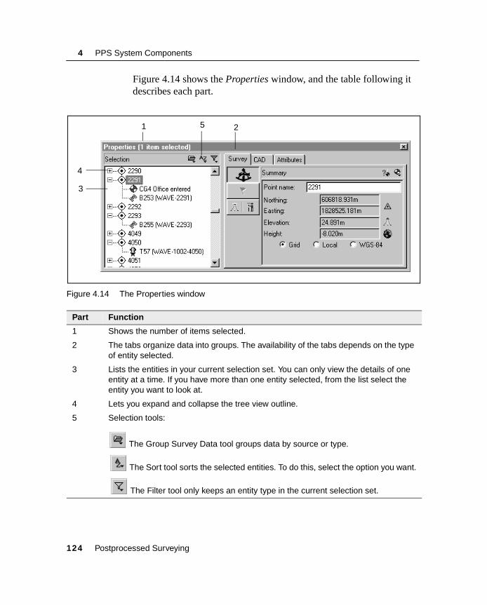
4 PPS System Components
Figure 4.14 shows the Properties window, and the table following it describes each part.
Figure 4.14 The Properties window
Part Function
1 Shows the number of items selected.
2 The tabs organize data into groups. The availability of the tabs depends on the type of entity selected.
3 Lists the entities in your current selection set. You can only view the details of one entity at a time. If you have more than one entity selected, from the list select the entity you want to look at.
4 Lets you expand and collapse the tree view outline.
5 Selection tools:
The Group Survey Data tool groups data by source or type.
The Sort tool sorts the selected entities. To do this, select the option you want.
The Filter tool only keeps an entity type in the current selection set.
1 2
3
4
5
124 Postprocessed Surveying

PPS System Components 4
The information and tabs available on the right side of the Properties window depend on the entity type currently selected. The following sections describe how to use the Properties window to view and edit data for each type.
4.26 Viewing Survey Data in the Properties windowUse the Survey tab of the Properties window to view and edit the survey-related properties of an entity in the selection. You can view the properties of entities that appear in the Survey view such as:
• Points
• GPS observations
• Conventional observations
• Level observations
• Laser rangefinder observations
• Azimuth observations
• Reduced observations
• Staked-out point information
• Events data
Postprocessed Surveying 125
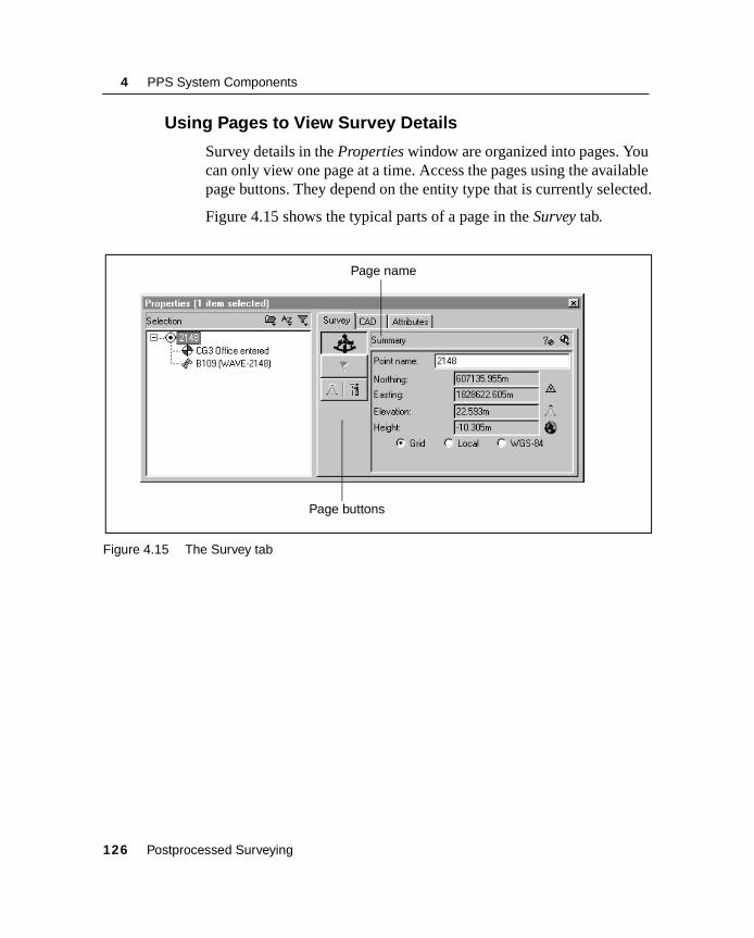
4 PPS System Components
4.26.1 Using Pages to View Survey Details
Survey details in the Properties window are organized into pages. You can only view one page at a time. Access the pages using the available page buttons. They depend on the entity type that is currently selected.
Figure 4.15 shows the typical parts of a page in the Survey tab.
Figure 4.15 The Survey tab
Page buttons
Page name
126 Postprocessed Surveying

PPS System Components 4
4.27 Viewing and Editing PointsPoint details in the Properties window are organized into the following tabs:
• Use the Survey tab to view and edit the survey-related details of a selected point.
• Use the Stakeout tab to view details about staked out points.
• Use the CAD tab to view and edit the CAD-related details of a selected point.
• If a selected point contains attribute information and you have set up the project for attributes, use the Attributes tab to view this information.
To view and edit the details of a point, select the appropriate tab in the Properties window.
The following sections describe the details of a point that you can view, using the Properties window.
Postprocessed Surveying 127

4 PPS System Components
4.27.1 Viewing Survey Details
Use the Survey tab in the Properties window to view and edit the survey-related details of the selected point (for example, the derived position, warning messages, occupation and setup details, coordinates, and observation statistics).
To view the survey details for a point:
1. In the Properties window, do one of the following:
– From the Properties window selection list, select a point.
– In the graphics window, select a point.
2. Select the Survey tab.
To select the types of survey details that you want to view, click a page button.
B Tip – To view the from and to points for any observation, click the plus (+) icon beside the observation. Then, click the point that you want to view and edit.
The following Properties window shows a typical page for a point:
128 Postprocessed Surveying

PPS System Components 4
Table 4.11 summarizes the pages for points in the Properties window. For more information on each page, refer to the appropriate Help topics.
Table 4.11 Pages for points in the Properties window
Button Page name What it shows
Summary The point name, the derived position, and qualities for a point.
Use this page to view the qualities of the position components or report on how the point was derived.
Warning A warning message indicating that a misclosure has been detected on the point, or that a high RMS was detected.
Use this page to view the error message and to suppress the warning flags displayed in the graphics window if the error is acceptable for the project.
Occupations and Setups
Details of any GPS occupation or terrestrial setup from or to the point.
Use this page to view and correct the details for the GPS occupation or terrestrial setup details, for example, antenna and target heights. If there is more than one occupation or setup for the point, a shortcut menu appears. As you hold the pointer over different occupations and setups in the shortcut menu, the occupation and setup details are updated in the page.
Error Estimate The estimated errors for the point’s position after a network adjustment, if you have the Network Adjustment module installed.
N/A Coordinate The underlying coordinates and qualities for a point.
Use this page to change the coordinate qualities and status of the point.
N/A GPS Solution (APC)
The position solution of a GPS point including the time of occupation, WGS-84 coordinates, and precisions.
Use this page to view the position solution and to change the status of the point.
Postprocessed Surveying 129
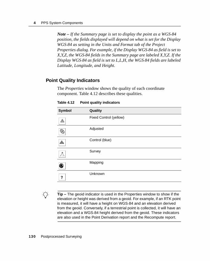
4 PPS System Components
Note – If the Summary page is set to display the point as a WGS-84 position, the fields displayed will depend on what is set for the Display WGS-84 as setting in the Units and Format tab of the Project Properties dialog. For example, if the Display WGS-84 as field is set to X,Y,Z, the WGS-84 fields in the Summary page are labeled X,Y,Z. If the Display WGS-84 as field is set to L,L,H, the WGS-84 fields are labeled Latitude, Longitude, and Height.
4.27.2 Point Quality Indicators
The Properties window shows the quality of each coordinate component. Table 4.12 describes these qualities.
B Tip – The geoid indicator is used in the Properties window to show if the elevation or height was derived from a geoid. For example, if an RTK point is measured, it will have a height on WGS-84 and an elevation derived from the geoid. Conversely, if a terrestrial point is collected, it will have an elevation and a WGS-84 height derived from the geoid. These indicators are also used in the Point Derivation report and the Recompute report.
Table 4.12 Point quality indicators
Symbol Quality
Fixed Control (yellow)
Adjusted
Control (blue)
Survey
Mapping
Unknown
130 Postprocessed Surveying
PPS System Components 4
4.28 Viewing ObservationsYou can view the survey details of any observation type, such as:
• GPS observations
• Conventional observations
• Level observations
• Laser rangefinder observations
• Azimuth observations
• Reduced observations
The following sections describe how to use the Properties window to view the survey details for each observation type.
4.28.1 GPS Observations
Use the Properties window to view the details of any GPS observation type such as RTK, Static, FastStatic and postprocessed kinematic baselines.
To view the survey details of an observation:
1. In the Properties window, do one of the following:
– From the Properties window selection list, select a GPS observation.
– In the graphics window, select a GPS observation.
2. To select the types of survey details that you want to view, click a page button.
B Tip – To view an observation from or to a point, click the plus (+) icon beside the point. Then, click the observation that you want to view.
Postprocessed Surveying 131
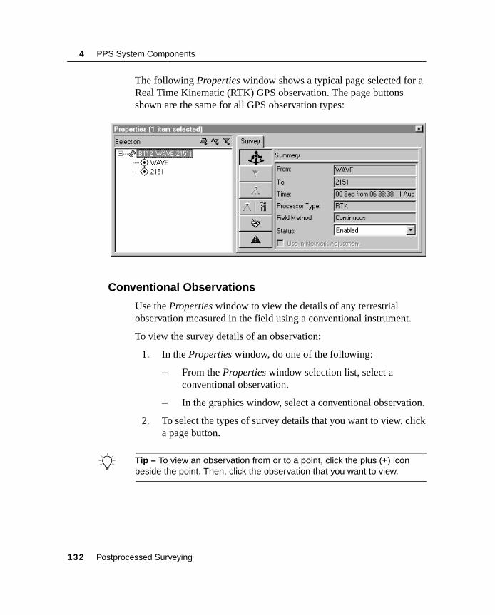
4 PPS System Components
The following Properties window shows a typical page selected for a Real Time Kinematic (RTK) GPS observation. The page buttons shown are the same for all GPS observation types:
4.28.2 Conventional Observations
Use the Properties window to view the details of any terrestrial observation measured in the field using a conventional instrument.
To view the survey details of an observation:
1. In the Properties window, do one of the following:
– From the Properties window selection list, select a conventional observation.
– In the graphics window, select a conventional observation.
2. To select the types of survey details that you want to view, click a page button.
B Tip – To view an observation from or to a point, click the plus (+) icon beside the point. Then, click the observation that you want to view.
132 Postprocessed Surveying

PPS System Components 4
The following Properties window shows a typical page selected for a conventional observation:
For more information about viewing other observation types, refer to the Trimble Geomatics Office help or manuals.
Postprocessed Surveying 133
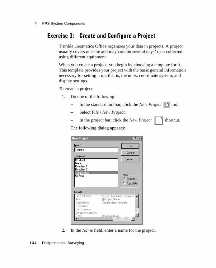
4 PPS System Components
Exercise 3: Create and Configure a Project
Trimble Geomatics Office organizes your data in projects. A project usually covers one site and may contain several days’ data collected using different equipment.
When you create a project, you begin by choosing a template for it. This template provides your project with the basic general information necessary for setting it up; that is, the units, coordinate system, and display settings.
To create a project:
1. Do one of the following:
– In the standard toolbar, click the New Project tool.
– Select File / New Project.
– In the project bar, click the New Project shortcut.
The following dialog appears:
2. In the Name field, enter a name for the project.
134 Postprocessed Surveying

PPS System Components 4
3. In the Template list, select a template. This determines the initial state of the project. The details of the selected template are displayed in the details list.
4. In the New group, make sure that the Project option is selected.
5. If you want the project files stored in a particular folder (other than that specified during installation), do the following:
a. Click Folder.
b. Specify the appropriate folder and then click OK.
The folder name appears in the Details list.
6. Click OK.
The project is created and the Project Properties dialog appears. The settings in this dialog are from the template selected for the project.
4.29 Changing the Project PropertiesUse the tabs in the Project Properties dialog to change a project’s properties, if necessary.
To access this dialog:
• Select File / Project Properties.
Postprocessed Surveying 135
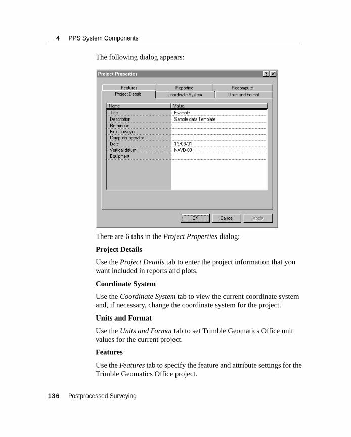
4 PPS System Components
The following dialog appears:
There are 6 tabs in the Project Properties dialog:
Project Details
Use the Project Details tab to enter the project information that you want included in reports and plots.
Coordinate System
Use the Coordinate System tab to view the current coordinate system and, if necessary, change the coordinate system for the project.
Units and Format
Use the Units and Format tab to set Trimble Geomatics Office unit values for the current project.
Features
Use the Features tab to specify the feature and attribute settings for the Trimble Geomatics Office project.
136 Postprocessed Surveying

PPS System Components 4
Reporting
Use the Reporting tab to control how you are notified when a system-generated report has been created.
Recompute
Use the Recompute tab to specify how Trimble Geomatics Office determines the calculated positions for all points in the project.
For more information, refer to the Trimble Geomatics Office User Guide.
Postprocessed Surveying 137

4 PPS System Components
4.30 Using Project TemplatesTo configure the initial state of a project, you must select a project template. To reduce the time required to configure new projects, create your own templates with the properties and data that are common to all of your projects.
4.30.1 Selecting a Template for a Project
When you create a new project, you must select a template. Using templates in Trimble Geomatics Office is similar to using template documents in Microsoft Word, or prototype drawings in AutoCAD. Trimble Geomatics Office templates are stored in C:\Program Files\Trimble\Trimble Geomatics Office\Template.
When a project is created, the whole template—including the template folders—is copied to the new project. For example, if an ASCII file containing control points exists in the template Checkin folder, the same file is copied to the Checkin folder of the project. The template you use stays the same. That is, any edits made to the project are not made to the template.
138 Postprocessed Surveying

PPS System Components 4
4.30.2 Creating a Template
To create a project template:
1. Select File / New Project. The New Project dialog appears.
2. In the New group, select the Template option. Project Folder in the Details list changes to Templates Folder, as shown below:
3. Enter a name for the new template.
4. Select an existing template on which to base the new one and then click OK. The Project Properties dialog appears.
5. Use the tabs in the Project Properties dialog to edit the default settings that Trimble Geomatics Office uses when creating a project based on the template.
6. Click OK. A message appears. It asks if you want to continue editing the template.
Postprocessed Surveying 139

4 PPS System Components
7. Do one of the following:
– To continue editing the template, click Yes. You can edit the template using parts of Trimble Geomatics Office other than the Project Properties dialog, for example, to enter common control points.
– To close the template, click No.
Note – You do not have to manually save a template. All changes to a template are automatically saved as they occur.
The new template appears in the Templates list when you create a new project. You can open a template in the same way that you would a project.
140 Postprocessed Surveying

PPS System Components 4
Exercise 4: Enter Coordinates for a Point
You can enter control coordinates for a point into Trimble Geomatics Office by:
• importing a Trimble Survey Controller job with keyed-in control coordinates entered in the field. For more information, refer to the Trimble Survey Controller documentation.
• importing an ASCII file with control points. For more information, refer to the Trimble Geomatics Office User Guide.
• entering known coordinates for an existing point using the Properties window or the Points dialog (if you have the Network Adjustment module installed). For information on using the Points dialog, refer to the Network Adjustment module Help.
• entering known coordinates for a new point using the Insert Points dialog. For more information, refer to the Trimble Geomatics Office User Guide.
Any coordinates entered receive an office-entered coordinate source. This is shown in the Properties window.
Note – Each point in Trimble Geomatics Office can only have one keyed-in WGS-84 coordinate and one keyed-in grid/local coordinate.
The following section describes how to use the Properties window to enter known coordinates for an existing point.
Using the Properties window to enter coordinates for a point
You can key in coordinates for a point using the Properties window. However, only do this when you want the software to use your keyed-in coordinate in preference to the coordinates derived from observations. The keyed-in coordinate will have an office-entered source.
Postprocessed Surveying 141
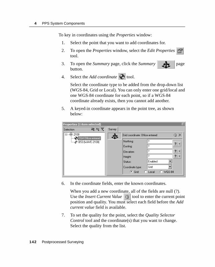
4 PPS System Components
To key in coordinates using the Properties window:
1. Select the point that you want to add coordinates for.
2. To open the Properties window, select the Edit Properties tool.
3. To open the Summary page, click the Summary page button.
4. Select the Add coordinate tool.
Select the coordinate type to be added from the drop-down list (WGS-84, Grid or Local). You can only enter one grid/local and one WGS-84 coordinate for each point, so if a WGS-84 coordinate already exists, then you cannot add another.
5. A keyed-in coordinate appears in the point tree, as shown below:
6. In the coordinate fields, enter the known coordinates.
When you add a new coordinate, all of the fields are null (?). Use the Insert Current Value tool to enter the current point position and quality. You must select each field before the Add current value field is available.
7. To set the quality for the point, select the Quality Selector Control tool and the coordinate(s) that you want to change. Select the quality from the list.
142 Postprocessed Surveying
PPS System Components 4
8. Use the Coordinate Type option to store the data in the database in the format specified. The software saves the coordinate in the coordinate view selected.
Note – You can only edit the coordinates in the display format that is stored in the database.
Note – If you have a keyed-in grid coordinate and a keyed-in WGS-84 coordinate, you cannot save the keyed-in grid coordinate as a WGS-84 coordinate.
Changing the status of coordinates
To change the status of an underlying coordinate using the Properties window, in a Coordinate page:
1. In the Status field, select the appropriate option. Do one of the following:
– If you want the coordinate used to derive the position of the point, select Enabled.
– If you do not want the coordinate used to derive the position of the point, select Disabled.
– If you only want the coordinate used if there are no other enabled observations or coordinates that can be used to derive the position of the point, select Enabled as check.
2. Click OK.
The software performs a recomputation, and you can view the new derived position for the point in the Summary page of the Properties window.
Note – The Recompute report reports on coordinates enabled as check, but not on disabled coordinates.
Postprocessed Surveying 143

4 PPS System Components
4.31 Trimble Data Transfer UtilityTrimble Geomatics Office uses Data Transfer to transfer data to or from the following devices:
• a data collector running Trimble Survey Controller
• a survey data card
• a Trimble GPS receiver
• a Trimble total station
• an SDR data recorder
You can also use the Data Transfer utility as standalone software to transfer data without using Trimble Geomatics Office.
To use the Data Transfer utility, you need the correct cables for connecting your device to your computer. For information about the cables you need, refer to the documentation for the device you are using.
The following sections describe the basic functions of the Data Transfer utility when accessed from Trimble Geomatics Office. For more information, refer to the Data Transfer Help.
For information about using the Data Transfer utility to transfer files, refer to the Trimble Survey Controller or Geomatics Office User Guides.
4.31.1 Using Data Transfer from Trimble Geomatics Office
The Data Transfer utility starts whenever you use the Export or Import dialogs to transfer files to or from a Trimble device. For example, to open the utility you can select the Feature and Attribute Library (*.fcl) to Survey Controller option in the Export dialog.
144 Postprocessed Surveying

PPS System Components 4
4.31.2 Using the Standalone Data Transfer Utility
You can use the Data Transfer utility as a standalone utility. Do one of the following:
• Click and then select Programs / Trimble Geomatics Office / Trimble Utilities / Data Transfer.
• When there is no project open, select Utilities / Data Transfer.
• When there is no project open, in the project bar, click the Utilities group and then click the Data Transfer shortcut.
This lets you transfer any file type to any device.
4.31.3 Setting Up Devices Using the Data Transfer Utility
Before using Data Transfer to transfer files between Trimble Geomatics Office and a device, you may need to set up a device. You can set up the following types of device:
• a data collector running Trimble Survey Controller
• a survey data card
• a Trimble GPS receiver
• a Trimble total station
• an SDR data recorder
Devices are system wide—once you have set up a device, it is available in all projects.
The following sections show you how to set up a Trimble Survey Controller device, a GPS receiver device and a survey data card device.
Postprocessed Surveying 145
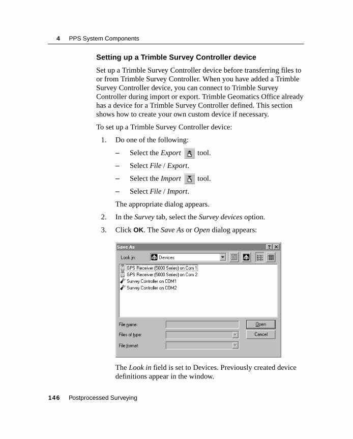
4 PPS System Components
Setting up a Trimble Survey Controller device
Set up a Trimble Survey Controller device before transferring files to or from Trimble Survey Controller. When you have added a Trimble Survey Controller device, you can connect to Trimble Survey Controller during import or export. Trimble Geomatics Office already has a device for a Trimble Survey Controller defined. This section shows how to create your own custom device if necessary.
To set up a Trimble Survey Controller device:
1. Do one of the following:
– Select the Export tool.
– Select File / Export.
– Select the Import tool.
– Select File / Import.
The appropriate dialog appears.
2. In the Survey tab, select the Survey devices option.
3. Click OK. The Save As or Open dialog appears:
The Look in field is set to Devices. Previously created device definitions appear in the window.
146 Postprocessed Surveying
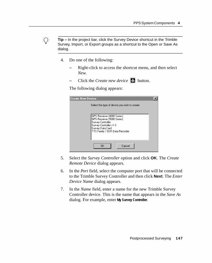
PPS System Components 4
B Tip – In the project bar, click the Survey Device shortcut in the Trimble Survey, Import, or Export groups as a shortcut to the Open or Save As dialog.
4. Do one of the following:
– Right-click to access the shortcut menu, and then select New.
– Click the Create new device button.
The following dialog appears:
5. Select the Survey Controller option and click OK. The Create Remote Device dialog appears.
6. In the Port field, select the computer port that will be connected to the Trimble Survey Controller and then click Next. The Enter Device Name dialog appears.
7. In the Name field, enter a name for the new Trimble Survey Controller device. This is the name that appears in the Save As dialog. For example, enter My Survey Controller.
Postprocessed Surveying 147
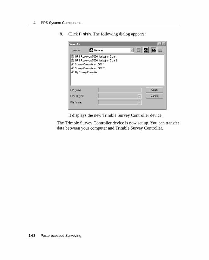
4 PPS System Components
8. Click Finish. The following dialog appears:
It displays the new Trimble Survey Controller device.
The Trimble Survey Controller device is now set up. You can transfer data between your computer and Trimble Survey Controller.
148 Postprocessed Surveying
PPS System Components 4
Setting up a GPS receiver device
Set up a GPS receiver device before transferring files from a GPS receiver. Once you add a GPS receiver device, you can connect to a GPS receiver device when you import.
To set up a GPS receiver device:
1. Do one of the following:
– Select the Import tool.
– Select File / Import.
The Import dialog appears.
2. In the Survey tab, select the Survey devices option and click OK. The Open dialog appears. The Look in field is set to Devices and previously created devices appear in the window.
B Tip – In the project bar, you can also click the Survey Device shortcut in the Trimble Survey or Import groups to display the Open dialog.
3. Do one of the following:
– Right-click to access the shortcut menu, and select New.
– Click the Create new device button.
The Create New Device dialog appears.
4. Select the GPS receiver (5000 Series) option and click OK. The Create Remote Device dialog appears.
Note – You can only use the GPS Receiver 5000 option to connect to a 5000 series receiver, that is, the 5700 receiver. To connect to a 4000 series receiver, use the GPS Receiver 4000 option.
5. In the Port field, select the computer port you use to connect to your GPS receiver and then click Next. The Enter Device Name dialog appears.
Postprocessed Surveying 149
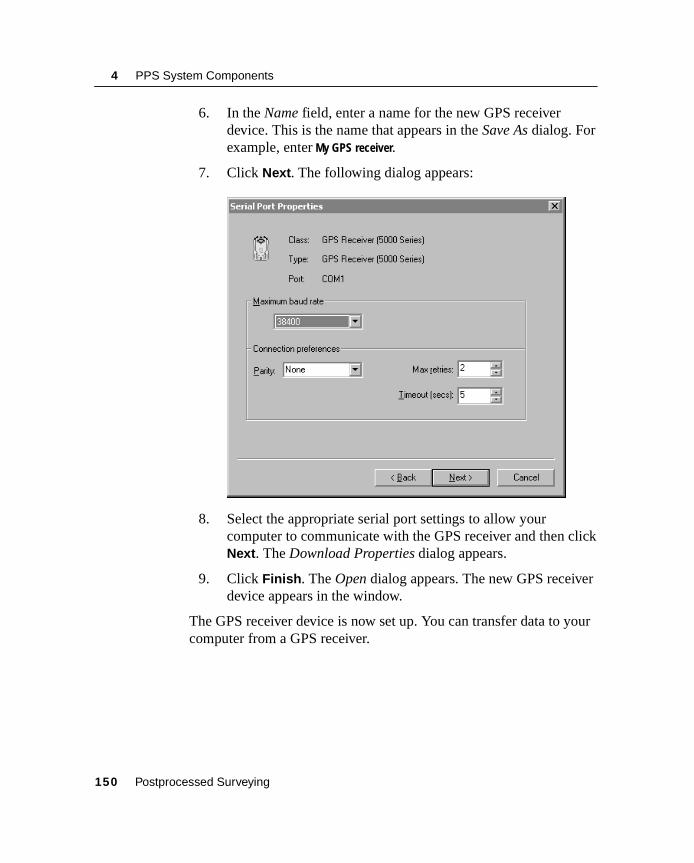
4 PPS System Components
6. In the Name field, enter a name for the new GPS receiver device. This is the name that appears in the Save As dialog. For example, enter My GPS receiver.
7. Click Next. The following dialog appears:
8. Select the appropriate serial port settings to allow your computer to communicate with the GPS receiver and then click Next. The Download Properties dialog appears.
9. Click Finish. The Open dialog appears. The new GPS receiver device appears in the window.
The GPS receiver device is now set up. You can transfer data to your computer from a GPS receiver.
150 Postprocessed Surveying
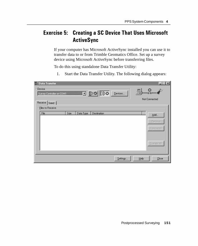
PPS System Components 4
Exercise 5: Creating a SC Device That Uses Microsoft
ActiveSync
If your computer has Microsoft ActiveSync installed you can use it to transfer data to or from Trimble Geomatics Office. Set up a survey device using Microsoft ActiveSync before transferring files.
To do this using standalone Data Transfer Utility:
1. Start the Data Transfer Utility. The following dialog appears:
Postprocessed Surveying 151
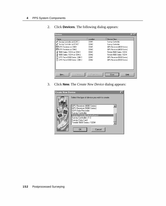
4 PPS System Components
2. Click Devices. The following dialog appears:
3. Click New. The Create New Device dialog appears:
152 Postprocessed Surveying

PPS System Components 4
4. Select the Survey Controller (ActiveSync) option and click OK. The Enter Device Name dialog appears:
5. In the Name field, enter a name for the new survey data card device. This is the name that appears in the Save As dialog. For example, enter SC 10 with AcitveSync.
Postprocessed Surveying 153
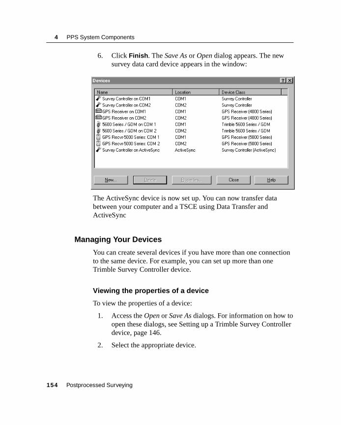
4 PPS System Components
6. Click Finish. The Save As or Open dialog appears. The new survey data card device appears in the window:
The ActiveSync device is now set up. You can now transfer data between your computer and a TSCE using Data Transfer and ActiveSync
4.31.4 Managing Your Devices
You can create several devices if you have more than one connection to the same device. For example, you can set up more than one Trimble Survey Controller device.
Viewing the properties of a device
To view the properties of a device:
1. Access the Open or Save As dialogs. For information on how to open these dialogs, see Setting up a Trimble Survey Controller device, page 146.
2. Select the appropriate device.
154 Postprocessed Surveying
PPS System Components 4
3. Right-click to access the shortcut menu, and select Properties. The appropriate Properties dialog appears. If a field is unavailable, that setting is not applicable for the device.
4. Edit the Properties dialog as required and click OK to apply your changes. The Open or Save As dialog returns.
Deleting a device
To delete a device at any time:
1. Access the Open or Save As dialogs. For information on how to open these dialogs, see Setting up a Trimble Survey Controller device, page 146.
2. Select the appropriate device and press [Delete] .
The following message appears:
Are you sure you want to delete ‘<device name>’?
Do one of the following:
– To delete the device, click Yes. The device is removed from the list in the dialog.
– To cancel the delete, click No. You are returned to the dialog
4.31.5 Importing ASCII Data Files
This section describes how to import an ASCII file into a Trimble Geomatics Office project.
You can import a variety of data file formats into Trimble Geomatics Office, as well as define your own custom ASCII formats to import. For example, you may have a data file containing control points that you want to import into Trimble Geomatics Office. If you have a data file containing design points that you want to stake out using Trimble Survey Controller, you need to import the data file into your Trimble Geomatics Office project, then transfer the points in a Trimble Survey Controller (*.dc) file to Trimble Survey Controller.
Postprocessed Surveying 155

4 PPS System Components
Using drag-and-drop
You can use Windows Explorer and the Microsoft Windows drag-and-drop functionality to import data files from a folder on your computer into a project.
To do this:
1. Open Windows Explorer. For more information, refer to your Windows operating system documentation.
2. Locate the folder containing the file that you want to import.
3. Use the right mouse button to drag the file onto the Trimble Geomatics Office graphics window. The shortcut menu appears, as shown below:
4. Select the option that matches the file format that you are importing. If the file format you require does not appear in the list, then Trimble Geomatics Office does not recognize the file format.
To import a file of this type, do one of the following:
– Define a custom import format.
– Use an import filter.
The software imports the file. For more information, refer to the Trimble Geomatics Office User Guide.
156 Postprocessed Surveying

PPS System Components 4
B Tip – If you use the left mouse button to drag-and-drop a file, Trimble Geomatics Office uses the extension of the file to determine the file that you are importing. If the file extension is used for more than one import format, the software uses the default format. If you do not know what the default format is, use the right mouse button and select the correct file format.
Postprocessed Surveying 157
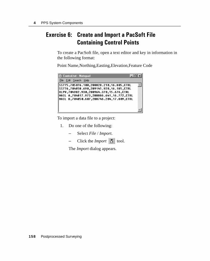
4 PPS System Components
Exercise 6: Create and Import a PacSoft File
Containing Control Points
To create a PacSoft file, open a text editor and key in information in the following format:
Point Name,Northing,Easting,Elevation,Feature Code
To import a data file to a project:
1. Do one of the following:
– Select File / Import.
– Click the Import tool.
The Import dialog appears.
158 Postprocessed Surveying
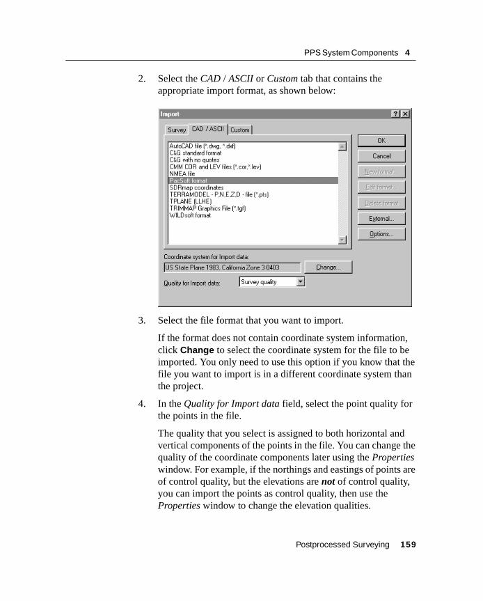
PPS System Components 4
2. Select the CAD / ASCII or Custom tab that contains the appropriate import format, as shown below:
3. Select the file format that you want to import.
If the format does not contain coordinate system information, click Change to select the coordinate system for the file to be imported. You only need to use this option if you know that the file you want to import is in a different coordinate system than the project.
4. In the Quality for Import data field, select the point quality for the points in the file.
The quality that you select is assigned to both horizontal and vertical components of the points in the file. You can change the quality of the coordinate components later using the Properties window. For example, if the northings and eastings of points are of control quality, but the elevations are not of control quality, you can import the points as control quality, then use the Properties window to change the elevation qualities.
Postprocessed Surveying 159
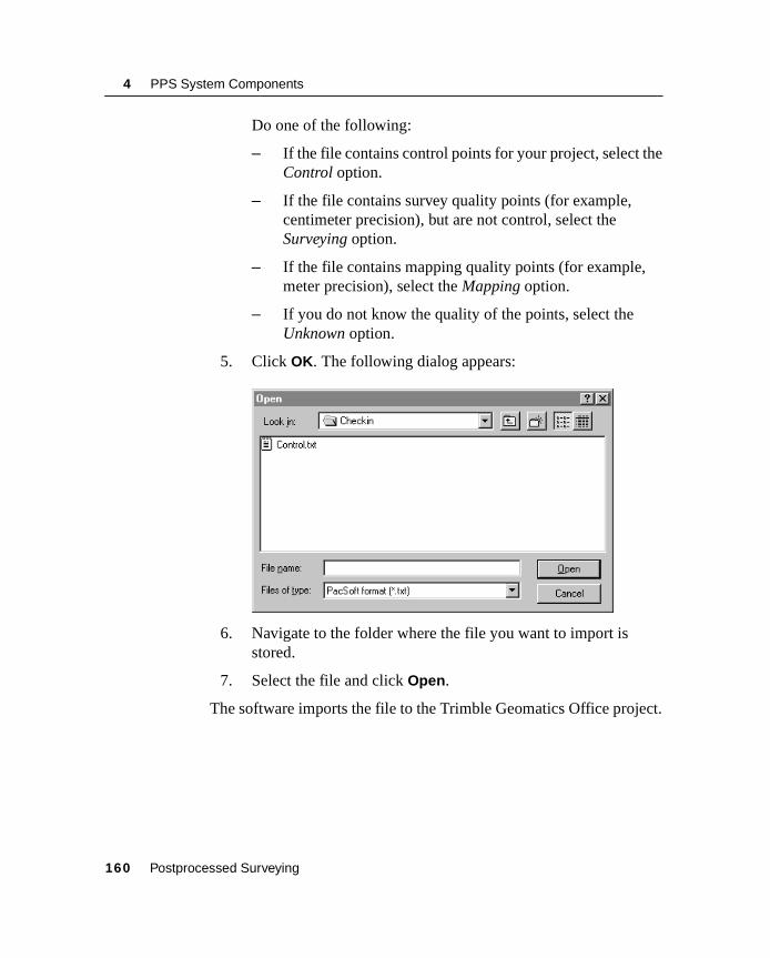
4 PPS System Components
Do one of the following:
– If the file contains control points for your project, select the Control option.
– If the file contains survey quality points (for example, centimeter precision), but are not control, select the Surveying option.
– If the file contains mapping quality points (for example, meter precision), select the Mapping option.
– If you do not know the quality of the points, select the Unknown option.
5. Click OK. The following dialog appears:
6. Navigate to the folder where the file you want to import is stored.
7. Select the file and click Open.
The software imports the file to the Trimble Geomatics Office project.
160 Postprocessed Surveying

PPS System Components 4
Exercise 7: Transfer Files to Trimble Survey Controller
To transfer files to Trimble Survey Controller:
1. Do one of the following:
– Select the Export tool.
– Select File / Export.
The following dialog appears:
2. In the Survey tab, select Survey Devices option.
Postprocessed Surveying 161
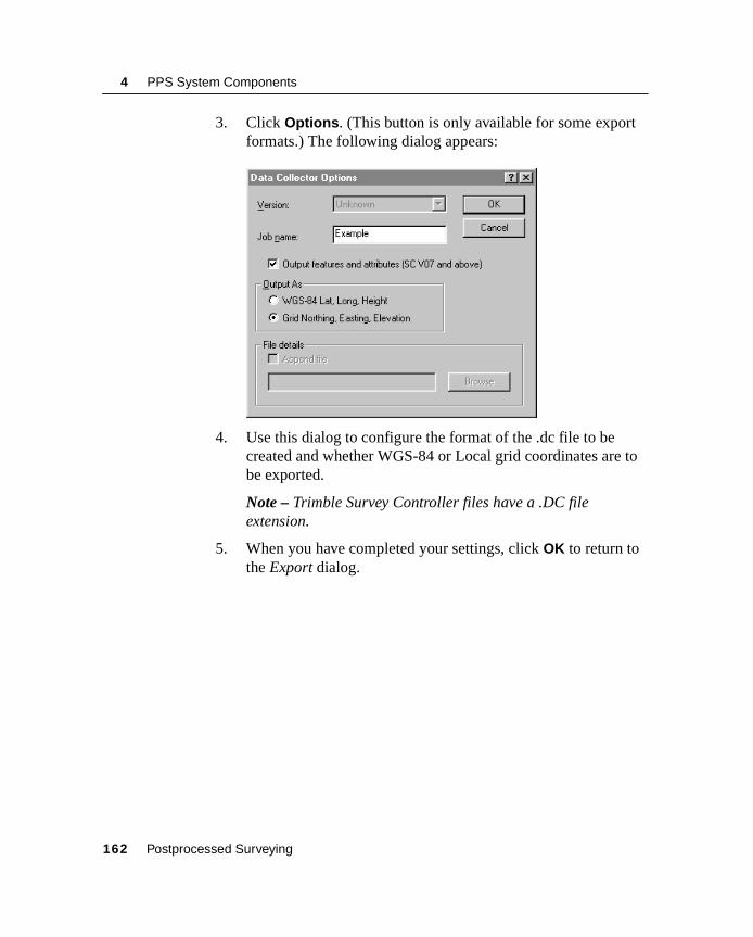
4 PPS System Components
3. Click Options. (This button is only available for some export formats.) The following dialog appears:
4. Use this dialog to configure the format of the .dc file to be created and whether WGS-84 or Local grid coordinates are to be exported.
Note – Trimble Survey Controller files have a .DC file extension.
5. When you have completed your settings, click OK to return to the Export dialog.
162 Postprocessed Surveying

PPS System Components 4
6. Click OK. The following dialog appears:
Once you have checked that Trimble Survey Controller is connected to the correct COM port and is in the appropriate data transfer mode, you can export the data.
To transfer the .dc file:
1. In the Open dialog, select a Trimble Survey Controller device.
2. Click Open. The following dialog appears as the computer connects to Trimble Survey Controller:
When the computer makes a connection, the Save As dialog returns. The Look in field is set to the Trimble Survey Controller device that you are connected to.
Postprocessed Surveying 163
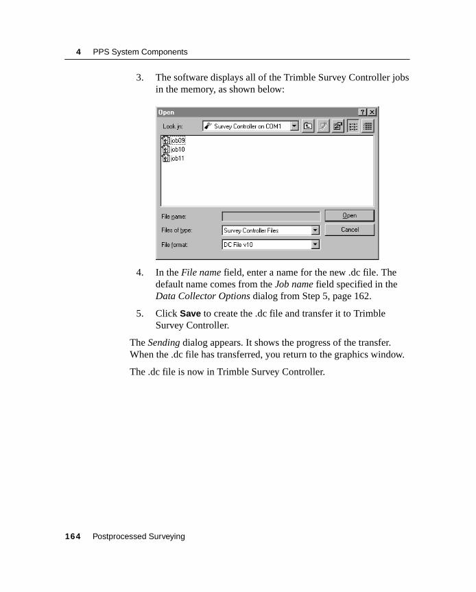
4 PPS System Components
3. The software displays all of the Trimble Survey Controller jobs in the memory, as shown below:
4. In the File name field, enter a name for the new .dc file. The default name comes from the Job name field specified in the Data Collector Options dialog from Step 5, page 162.
5. Click Save to create the .dc file and transfer it to Trimble Survey Controller.
The Sending dialog appears. It shows the progress of the transfer. When the .dc file has transferred, you return to the graphics window.
The .dc file is now in Trimble Survey Controller.
164 Postprocessed Surveying

PPS System Components 4
4.32 Review Questions1. What is the easiest way to configure Trimble Survey Controller?
2. What parameters must be defined before you start any project or job?
3. Where do you select the method in which your distances are displayed in Trimble Survey Controller: Grid, Ground, or Sea Level?
4. What is the easiest way to obtain information about Trimble Survey Controller operations when you are in the field?
5. What is an excellent source of information for processes in Trimble Geomatics Office?
6. Name the two views in Trimble Geomatics Office.
7. What is a template?
8. What menu options are used for bringing data into or out of your project database in Trimble Geomatics Office?
9. What is the difference between Data Transfer and Import/Export?
10. If Trimble Geomatics Office does not support your ASCII file format, what Import/Export option can you use to bring that file’s data into your project?
Postprocessed Surveying 165
4 PPS System Components
4.33 Answers1. Use Survey Styles, either Trimble’s or your own.
2. Define a map projection, local or published, datum transformation, horizontal and vertical adjustments, and geoid model.
3. Use Configuration / Job / Cogo Settings menu options, or from any distance field options.
4. Use the [Help] key.
5. Use the Help menu.
6. Plan and Survey view.
7. A template is a definable set of parameters that can be reused when starting a new project. The parameters include: units and format, coordinate system, and general settings.
8. Use the Import or Export options to bring data into or send it out of your project database.
9. Data Transfer is used to transfer data from or to your Trimble Survey Controller/PC card or receiver to your computer.Import/Export allows you to do the same and import or export data to or from your project database.
10. Use the Custom tab and generate your own import/export file format.
166 Postprocessed Surveying

C H A P T E R
5
Mission Planning 5In this chapter:
■ Introduction
■ Session objectives
■ Survey tasks
■ Review questions
■ Answers
■ Network design
■ Review questions
■ Answers

5 Mission Planning
5.1 IntroductionThis session describes the planning and design stages of a postprocessed survey, including the concepts of this phase of the project. It shows how to determine the best time to observe satellites, and how to design a network, given that there may be more than one suitable network design for a project.
Getting the planning and design right increases your chances of collecting high-quality data, and yielding accurate coordinates with a high degree of confidence.
5.2 Session ObjectivesAt the end of this session, you will be able to:
• Describe ways to obtain an almanac file.
• Perform a site reconnaissance and complete a site obstruction diagram
• Plan a session using the Trimble QuickPlanTM utility.
• Design a control network according to best practise guidelines.
168 Postprocessed Surveying

Mission Planning 5
5.3 Survey TasksThis section describes the tasks associated with planning a GPS survey:
• Session planning:
– Pre-survey preparation
– Site reconnaissance
– Survey planning
• Network Design
5.3.1 Pre-survey Preparation
As emphasized earlier in this manual, have a full understanding of your hardware capabilities. The functionality of your hardware defines which type of field procedures you can use while observing baselines.
Prepare a written plan of your project describing the purpose, scope of work, and ways you expect to collect and use the data. You may find that by collecting data on a few additional points you can considerably strengthen the network geometry. Also, collecting more data than is needed at the moment may yield valuable information for future use. For example, it could enable you to salvage a survey if you find gross errors in the observation of one or more baselines. Determine if observations on additional points are feasible for your current project.
Postprocessed Surveying 169

5 Mission Planning
5.3.2 Site Reconnaissance
This is an indispensable part of field survey planning, which comprises:
• Setting or recovering survey points for the field crew
• Noting the presence of obstructions that may affect observation scheduling or may require that you relocate survey points
• Obtaining permission to enter the job site from private property owners
• Determining the best way to reach each survey station (in any type of weather and at any time of the day or night)
• Drawing maps and write directions so that the survey crew can reach the job site and find the points to be observed
• Estimating travel time between stations
Note – (North America only) A good way to get location information if the point has not been observed yet is to take a receiver along and use WAAS positions to mark the station for recovery and assist in navigation to the point for observation later.
170 Postprocessed Surveying

Mission Planning 5
5.3.3 Survey Planning
Firstly, create the project in the Trimble Geomatics Office software. This will automatically create the subdirectories required for all further operations associated with the project and simplify the data management. Use the QuickPlan utility to plan the field observation portion of the project, in which you:
• create field observation sessions and define all of the stations you want to observe
• enter information from the obstruction diagrams that you drafted on your visit to each survey station
• compute the best field observation times
Postprocessed Surveying 171

5 Mission Planning
To determine the best time to observe satellites and collect high-quality data we require the QuickPlan utility and the following information:
• Almanac file
• Approximate coordinates of the project area
• Site obstruction diagrams
• Campaign period
• Local weather report
• GPS status message (optional)
Almanac/Ephemeris File
An almanac contains orbit data for all available satellites. Aids in rapid satellite acquisition and planning.
A broadcast ephemeris is predicted orbit data for an individual satellite, used in baseline processing. A broadcast ephemeris file is updated every two hours.
A precise ephemeris is precise, observed orbital parameters for an individual satellite, usually used for a high-precision geodetic survey with a very long baseline. This file is available about two weeks after observing data from various sources, including the National Geodetic Society (NGS) website: www.ngs.noaa.gov. For more information, refer to the Trimble Geomatics Office Help.
An almanac is a subset of the ephemeris data with reduced precision.
Trimble recommends that you use an almanac file no older than one month. You can obtain a current almanac:
• from Trimble’s website:
http://www.trimble.com/gpsdataresources.html
Almanac files are updated hourly on this page.
• by tracking satellites with a GPS receiver and downloading the file.
172 Postprocessed Surveying

Mission Planning 5
The QuickPlan utility uses the following ephemeris formats:
• EPH files (*.eph)
• SSF files (*.ssf)
• YUMA files (*.txt)
Project area
Determine the general location of your project area in WGS-84 geographic coordinates. The QuickPlan utility, located in the Trimble Utilities folder, helps determine satellite availability and position from the general project location.
Think about project logistics. Questions to consider:
• Where are control points located?
• How accessible are the control points?
• Are there better control points to use?
Solving logistical problems in the planning stages saves time in the field.
Obstructions
The GPS satellite signal is a radio frequency (RF) signal and can be blocked by obstacles such as hills, buildings, trees, and towers.
Those obstructions may temporarily obstruct one or more satellites during an observation and result in loss of lock in signal tracking. This temporary signal loss is called a cycle slip.
Cycle slips can be avoided by maintaining contact with four or more satellites at all times during observation. Adequate planning and use of obstruction diagrams will help avoid cycle slips.
The only way to verify obstructions is by performing a site reconnaissance.
Postprocessed Surveying 173
5 Mission Planning
When you visit a site and locate possible obstructions, record the azimuth and elevation of the obstructions relative to the survey point. Back at the office, the site obstruction information can be entered into the QuickPlan software to analyze the effect the obstructions may have on your point of observation.
Obstructions can also cause multipath interference.
Elevation mask
To help overcome interference from obstructions, use an elevation mask, which is a user-defined horizon below which the receiver does not record data. You can ignore obstructions that fall below the elevation mask. By default, the elevation mask in a GPS receiver is 13 degrees.
The elevation mask can also minimize atmospheric effects introduced into the GPS signal. Signals from satellites high in the sky travel through less dense atmosphere than satellite signals with lower elevations.
Any satellites below an elevation mask are not logged. It may be better, for sites you are unsure about, to leave the elevation mask at 13 for data collection, then set it higher for baseline processing.
GPS status message
The United States of America Department of Defense (DoD) maintains the GPS space segment by compiling information about satellite health. The United States Coast Guard (USCG) relays this information to GPS civilian users through the GPS Status Message.
The GPS Status Message includes information such as satellite health and scheduled satellite maintenance. This determines which satellites are available.
To obtain the GPS Status Message, subscribe to
• United States Coast Guard (USCG) Navigation Center electronic mailing lists (www.navcen.uscg.gov/)
174 Postprocessed Surveying

Mission Planning 5
Exercise 8: Extract an Almanac File from
a GPS Receiver
An almanac file is created by tracking satellites with a receiver and downloading the file to your computer. Trimble recommends tracking satellites for 40 minutes to obtain an almanac file. The current file can then be extracted from the Trimble receiver using the Data Transfer utility, located in Trimble Geomatics Office / Trimble Utilities.
To extract an almanac file:
1. Select Start / Programs / Trimble Geomatics Office / Trimble Utilities / Data Transfer.
2. Select the device you wish to communicate with, as shown in the following dialog:
3. Click Add.
4. Change the Files of type to Current Receiver Almanac.
5. Choose the appropriate destination folder for the file.
Postprocessed Surveying 175
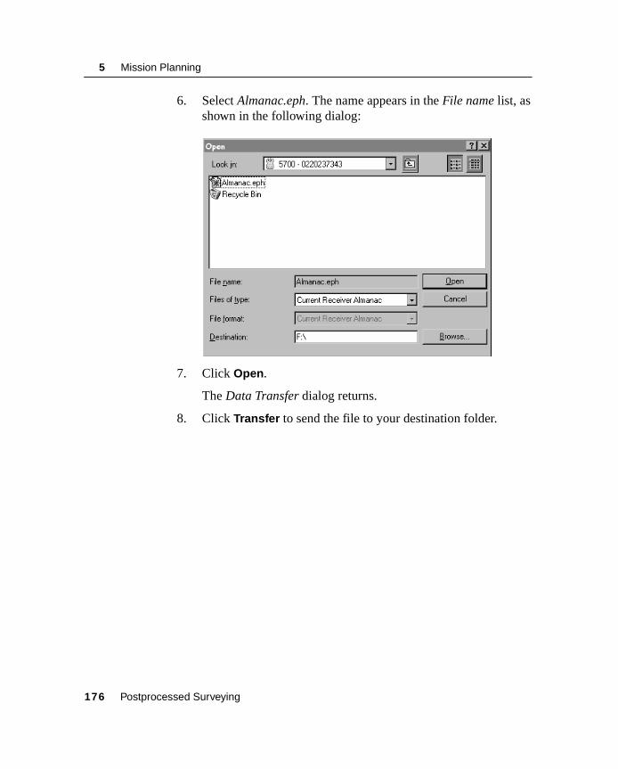
5 Mission Planning
6. Select Almanac.eph. The name appears in the File name list, as shown in the following dialog:
7. Click Open.
The Data Transfer dialog returns.
8. Click Transfer to send the file to your destination folder.
176 Postprocessed Surveying

Mission Planning 5
Exercise 9: Create a Site Obstruction Diagram
Your instructor will take you to a survey point. Use the following tables and Figure 5.1 to record all the site information needed to plan an occupation:
Station information
Station Name
Map Reference
Date Latitude
Observer Longitude
Directions to site
Site Description
Sketch
OBST # TYPE/DESCRIPTION FROM TO
AZ ELEV AZ ELEV
Postprocessed Surveying 177

5 Mission Planning
.
Figure 5.1 Site obstruction diagram
Station Name __________________________________________
B Tip – Photocopy this page and use it to create a site obstruction diagram.
178 Postprocessed Surveying
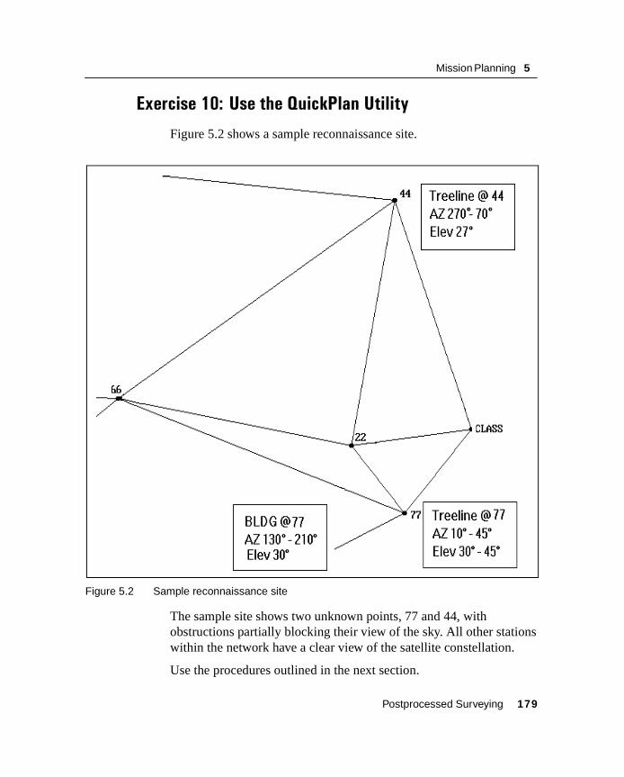
Mission Planning 5
Exercise 10: Use the QuickPlan Utility
Figure 5.2 shows a sample reconnaissance site.
Figure 5.2 Sample reconnaissance site
The sample site shows two unknown points, 77 and 44, with obstructions partially blocking their view of the sky. All other stations within the network have a clear view of the satellite constellation.
Use the procedures outlined in the next section.
Postprocessed Surveying 179

5 Mission Planning
5.3.4 Starting the QuickPlan Utility and Selecting a Date
To start the QuickPlan Utility:
1. Select Start / Programs / Trimble Geomatics Office / Trimble Utilities / QuickPlan.
2. Select the appropriate date from the calendar, as shown:
3. Click OK.
180 Postprocessed Surveying
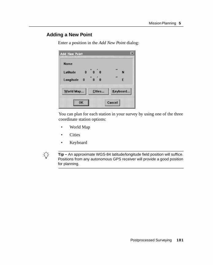
Mission Planning 5
5.3.5 Adding a New Point
Enter a position in the Add New Point dialog:
You can plan for each station in your survey by using one of the three coordinate station options:
• World Map
• Cities
• Keyboard
B Tip – An approximate WGS-84 latitude/longitude field position will suffice. Positions from any autonomous GPS receiver will provide a good position for planning.
Postprocessed Surveying 181
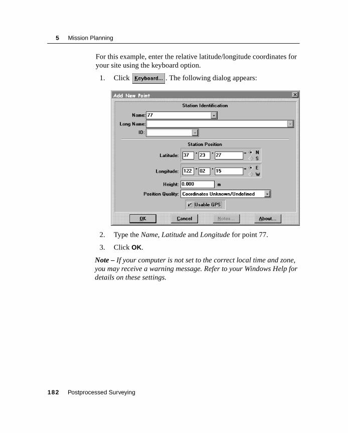
5 Mission Planning
For this example, enter the relative latitude/longitude coordinates for your site using the keyboard option.
1. Click . The following dialog appears:
2. Type the Name, Latitude and Longitude for point 77.
3. Click OK.
Note – If your computer is not set to the correct local time and zone, you may receive a warning message. Refer to your Windows Help for details on these settings.
182 Postprocessed Surveying

Mission Planning 5
5.3.6 Status Parameters
Check that your project parameters are correct in the QuickPlan Status window:
C Warning – You will need to update the Almanac to produce good planning information. To view the Status information at any time, select Options / Show Status.
Postprocessed Surveying 183

5 Mission Planning
5.3.7 Selecting an Almanac
To view satellite graphs, the QuickPlan utility needs to know satellite position. Although an almanac file is in the computer, you still need to select it. The almanac file is stored in the c:\Windows\Temp folder if you have used the default download process from a GPS receiver using the Data Transfer utility.
To load a current almanac file:
1. From the QuickPlan menu, select Options / Almanac.
2. Navigate to the drive and path of the ephemeris file. Use the List files of type and Drives drop-down lists.
3. Double-click the desired almanac file so that it appears as the selected file.
4. Click OK.
When you select an almanac file, the QuickPlan utility uses the satellite data for session planning. The Status window displays the almanac file and satellites used.
184 Postprocessed Surveying
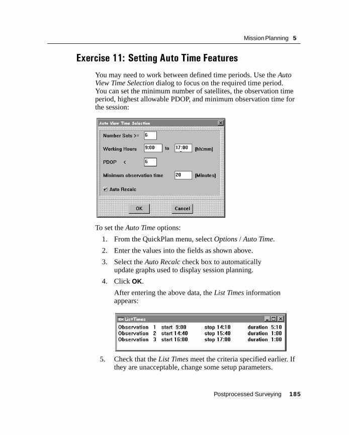
Mission Planning 5
Exercise 11: Setting Auto Time Features
You may need to work between defined time periods. Use the Auto View Time Selection dialog to focus on the required time period. You can set the minimum number of satellites, the observation time period, highest allowable PDOP, and minimum observation time for the session:
To set the Auto Time options:
1. From the QuickPlan menu, select Options / Auto Time.
2. Enter the values into the fields as shown above.
3. Select the Auto Recalc check box to automatically update graphs used to display session planning.
4. Click OK.
After entering the above data, the List Times information appears:
5. Check that the List Times meet the criteria specified earlier. If they are unacceptable, change some setup parameters.
Postprocessed Surveying 185

5 Mission Planning
Exercise 12: View Satellite Graphs
The QuickPlan utility provides graphs for viewing observation information using parameters set in the Auto View Time Selection dialog.
To view graphical information:
1. Select Graphs / Number SVs and PDOP to open the most useful graph, Number SVs and PDOP:
Hatched pink lines show times that meet the predefined criteria of the Auto View Time Selection dialog. Discontinuity in hatching indicates time that does not meet specifications.
The bar colors and vertical axis height indicate the quality of solution during the time shown on the horizontal axis:
• Red indicates fewer than four satellites available. Do not survey.
• Yellow indicates conditions are at minimum specifications.
• Green indicates good survey conditions.
• Blue indicates excellent conditions.
2. You can zoom into areas of the graph by double-clicking the left mouse button on the time displayed at the bottom of the graph. To zoom out, use the right mouse button.
3. Select File / Print to print graphs for use in the field.
186 Postprocessed Surveying

Mission Planning 5
Exercise 13: Edit a Session
Editing a session allows you to change parameters, such as the date, time, and position for the current session.
1. Select Session / Edit Session, as shown:
2. Highlight the desired session.
3. Click Edit.
4. Edit session information, for example, the date.
Note – Obstruction curtains can be added to your position from the Edit Session dialog.
5. Click OK.
Postprocessed Surveying 187

5 Mission Planning
Exercise 14: Define and View Curtains
(Point Obstructions)
Curtains are point obstructions blocking satellite signals. There are two types of curtains that can be defined in the QuickPlan utility:
• A single curtain is defined by left and right vertical boundaries and a constant elevation.
• A continuous curtain is defined by left and right vertical boundaries and a varied elevation.
For this example, you will apply curtains for the following two points:
• Point 77 has two curtains.
The first obstruction is a semi-deciduous tree blocking satellite signals from azimuth of 10° (measured clockwise from north) and elevation 30°, to azimuth of 45°, and elevation of 45°.
The other obstruction is a building, from azimuth of 130° to 210°, with a constant elevation of 30°.
• Point 44 has one curtain.
A tree-line obstruction blocks signals from azimuth of 270o to 70o azimuth with a constant elevation of 27o.
188 Postprocessed Surveying

Mission Planning 5
To define the curtains:
1. Select Session / New Session. The Add New Session dialog appears:
2. Double-click point 77 in the all points list.
Postprocessed Surveying 189

5 Mission Planning
3. Click to open the Curtain editor dialog:
4. In the Sky Coords group, click Cancel.
5. Select Edit / Edit Multiple Single Curtains.
Do not use your mouse to enter these curtains.
For the tree-line curtain, enter the following values into these fields:
a. Azimuth: 10. and then press [TAB].
b. Elevation: 30. and then press [ENTER].
c. Azimuth: 45. and then press [TAB].
d. Elevation: 45. and then press [ENTER].
Note – When curtains have been saved, they will affect the display of all graphs in the QuickPlan utility for further analysis of the current session.
190 Postprocessed Surveying

Mission Planning 5
For the building curtain, enter the following values into these fields:
1. Azimuth: 130. Press [Tab].
2. Elevation field: 30. Press [Enter].
3. Azimuth field: 210. Press [Tab].
4. Elevation: 30. Press [Enter].
If you need to clear curtains and start again:
1. Select File / New, from Curtain editor.
2. Click OK.
After creating all curtains:
1. In the Sky Coords group, click Cancel.
2. Click Save Curtain.
3. Select File / Exit.
Now create a curtain for point 44.
Postprocessed Surveying 191
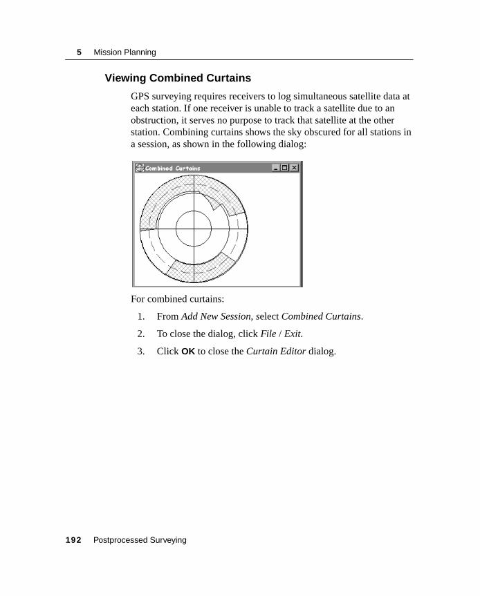
5 Mission Planning
5.3.8 Viewing Combined Curtains
GPS surveying requires receivers to log simultaneous satellite data at each station. If one receiver is unable to track a satellite due to an obstruction, it serves no purpose to track that satellite at the other station. Combining curtains shows the sky obscured for all stations in a session, as shown in the following dialog:
For combined curtains:
1. From Add New Session, select Combined Curtains.
2. To close the dialog, click File / Exit.
3. Click OK to close the Curtain Editor dialog.
192 Postprocessed Surveying
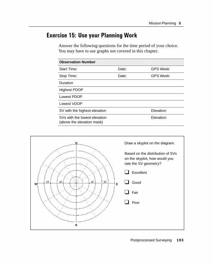
Mission Planning 5
Exercise 15: Use your Planning Work
Answer the following questions for the time period of your choice. You may have to use graphs not covered in this chapter.
Observation Number
Start Time: Date: GPS Week:
Stop Time: Date: GPS Week:
Duration
Highest PDOP
Lowest PDOP
Lowest VDOP
SV with the highest elevation Elevation:
SVs with the lowest elevation (above the elevation mask)
Elevation:
❑ Excellent
❑ Good
❑ Fair
❑ Poor
Draw a skyplot on the diagram.
Based on the distribution of SVson the skyplot, how would yourate the SV geometry?
Postprocessed Surveying 193

5 Mission Planning
5.4 Review Questions1. List two pieces of information required to plan a GPS
observation session.
2. How long must a receiver track satellites to obtain or update an almanac file?
3. How do you verify site obstructions?
4. What is a cycle slip?
5. What is an elevation mask and what is the default setting in a GPS receiver?
6. List three ways to add a point to a session.
7. Explain the value of creating curtains.
8. What does the QuickPlan utility require in order to know satellite positions?
9. Which graph or plot is most useful for selecting times to survey on a given day?
194 Postprocessed Surveying

Mission Planning 5
5.5 Answers1. Almanac file, approximate WGS-84 coordinate of the survey
area.
2. Trimble recommends 40 minutes.
3. Visit the site.
4. Temporary satellite signal loss.
5. A user-defined horizon which defines the lowest recorded satellite elevation; 13 degrees.
6. World map, cities, keyboard.
7. GPS surveying requires receivers log simultaneous SV data at each station. If a receiver cannot track a satellite because of an obstruction, the data from an unobstructed receiver cannot be used.
8. Almanac file.
9. Number of SVs and PDOP graph.
Postprocessed Surveying 195
5 Mission Planning
5.6 Network DesignA good network design is imperative for a successful control survey campaign. Even for those cases where GPS is used for topographic purposes, control points are required to tie the project to a common reference frame. Extra control points also act as reinitialization points if kinematic procedures are to be used and on-the-fly initialization is not available.
When designing your network, make a map of the stations, including both fixed-control and unknown points (to be observed). Because distance between points is an important factor, scale the map correctly.
Note – (North America only) If you collected WAAS or autonomous data during the reconnaissance phase, the map is already done.
Also, create an observation schedule that considers both the observation time for each station and the travel time between the stations.
196 Postprocessed Surveying

Mission Planning 5
5.6.1 The Purpose
Before designing a network, define the overall goal of your project. Design your network to achieve that goal with confidence.
Confidence in your network occurs when the network is free from field observation errors. Providing enough quality control checks identifies errors to remove them from the network.
The purpose of network design is to:
• Fulfill the requirements of the survey
• Optimize time spent in the field
• Provide checks on data collected
• Produce results with confidence
Postprocessed Surveying 197

5 Mission Planning
5.6.2 Network Design Guidelines
Use the following guidelines for good network design:
• Acquire control within project area
• Use good network geometry
• Incorporate independent baselines
• Build network redundancy
• Require two independent occupations per station
• Use stations with low multipath
• Do not let logistical constraints degrade your network design
198 Postprocessed Surveying
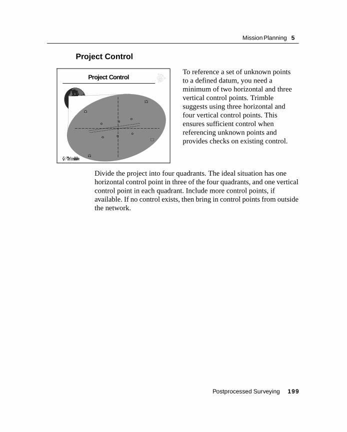
Mission Planning 5
5.6.3 Project Control
Divide the project into four quadrants. The ideal situation has one horizontal control point in three of the four quadrants, and one vertical control point in each quadrant. Include more control points, if available. If no control exists, then bring in control points from outside the network.
Project ControlTo reference a set of unknown points to a defined datum, you need a minimum of two horizontal and three vertical control points. Trimble suggests using three horizontal and four vertical control points. This ensures sufficient control when referencing unknown points and provides checks on existing control.
Postprocessed Surveying 199

5 Mission Planning
5.6.4 Network Geometry
A network design consists of a set of baselines between network points. The baselines have angular and spatial relationships amongst themselves. These relationships form the network geometry.
Good network geometry
Good geometry has good baseline distribution with a similar number of baselines going in and out of each point.
Good Network GeometryDesign all networks with good network geometry. Good network geometry contains small closed figures with less than six baselines. These figures allow you to perform loop closures. If the misclosure within a closed loop is high, it indicates a problem with at least one baseline within the loop. Performing additional loop closures isolates and identifies problematic baselines. Consequently, the bad baseline can be confidently removed.
200 Postprocessed Surveying

Mission Planning 5
Poor network geometry
Bad network geometry
Poor Network GeometryEven poor geometry allows you to perform loop closures. However, one loop closure using the same baselines only shows that a problem exists within the network. Without including the baseline in several loops, the geometry fails to isolate and identify the bad baselines in the network.
Bad Network GeometryComputing coordinates for unknown points with bad network geometry does not allow you to identify any existing network errors. Any one of those baselines could propagate error throughout the rest of the network.
Postprocessed Surveying 201

5 Mission Planning
5.6.5 Independent Baselines
The use of independent baselines ensures that all data is used only once. Dependent data can introduce a bias into a data set and give erroneous results.
If a GPS session uses five receivers, the raw data produces ten possible baselines. Only four of those baselines are independent. Independent baselines must not form a closed figure. The surveyor decides which four are independent.
Trivial or dependent baselines distort network statistics. Station accuracy statistics are falsely improved.
Independent Baselines
# of possible baselines = N(N - 1)2
# of independent baselines = N - 1
N = # of receivers
Formulas
202 Postprocessed Surveying

Mission Planning 5
5.6.6 Network Redundancy
Network RedundancyAdditional observations beyond the minimum required to compute coordinates for unknown points are called redundant observations. Redundancy in field measurements:
• Isolates and identifies errors
• Provides network quality control checks which increases confidence in the results
Trivial baselines are not redundant observations
Postprocessed Surveying 203
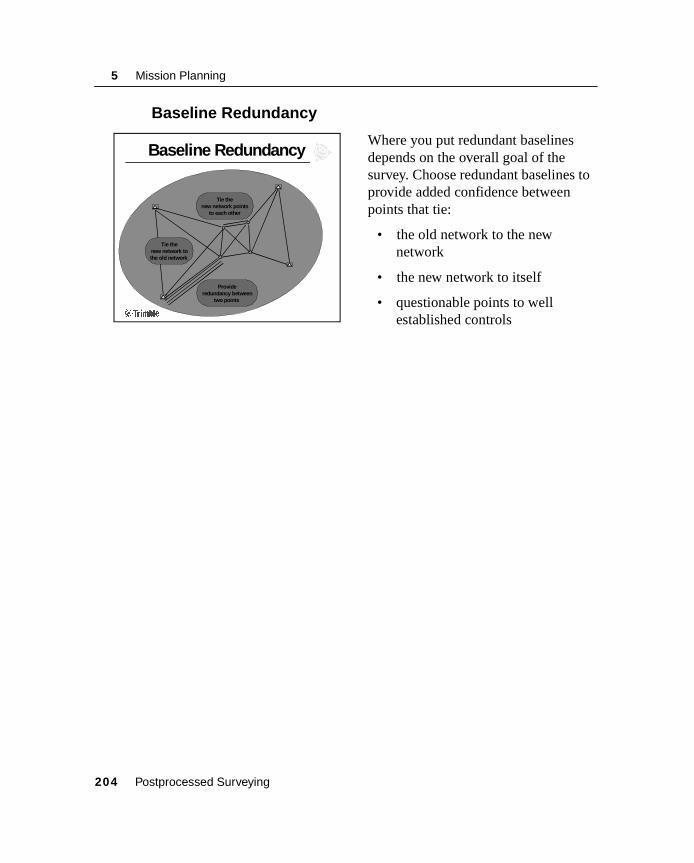
5 Mission Planning
5.6.7 Baseline Redundancy
Baseline Redundancy
Provideredundancy between
two points
Tie thenew network points
to each other
Tie thenew network tothe old network
Where you put redundant baselines depends on the overall goal of the survey. Choose redundant baselines to provide added confidence between points that tie:
• the old network to the new network
• the new network to itself
• questionable points to well established controls
204 Postprocessed Surveying
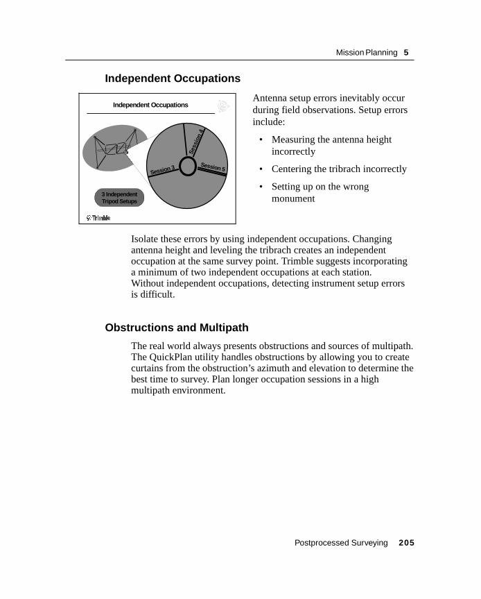
Mission Planning 5
5.6.8 Independent Occupations
Isolate these errors by using independent occupations. Changing antenna height and leveling the tribrach creates an independent occupation at the same survey point. Trimble suggests incorporating a minimum of two independent occupations at each station. Without independent occupations, detecting instrument setup errors is difficult.
5.6.9 Obstructions and Multipath
The real world always presents obstructions and sources of multipath. The QuickPlan utility handles obstructions by allowing you to create curtains from the obstruction’s azimuth and elevation to determine the best time to survey. Plan longer occupation sessions in a high multipath environment.
Independent Occupations
Session 3
Sess
ion
4
Session 5
3 IndependentTripod Setups
Antenna setup errors inevitably occur during field observations. Setup errors include:
• Measuring the antenna height incorrectly
• Centering the tribrach incorrectly
• Setting up on the wrong monument
Postprocessed Surveying 205

5 Mission Planning
5.6.10 Network Degradation
Many times you are forced to take shortcuts to finish a project quickly. Logistical constraints may compromise network integrity, forcing you to re-observe baselines in the field.
Extra surveying sessions improve redundancy, but network baselines must form closed loops. These closed figures reveal misclosure errors and isolate bad baseline data. Increase position confidence when viewing misclosure error in the Trimble Geomatics Office Network Adjustment module by planning a network which closes upon itself.
206 Postprocessed Surveying

Mission Planning 5
Exercise 16: Design a Network
The City of Sunnyvale has hired you to survey the network shown in Figure 5.3. For this exercise:
• You obtained horizontal and vertical control for CORTE, BM29, MARY, and 66.
• You are to derive precise coordinates for points PK1 and HUB2. Small-scale GPS and conventional surveys will use these points as control.
• Design a network that allows you to compute precise coordinates for the two unknown points.
• You have four receivers at your disposal.
• Use as few sessions as possible without compromising the integrity of the network.
Postprocessed Surveying 207
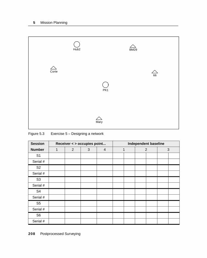
5 Mission Planning
Figure 5.3 Exercise 5 – Designing a network
Session Receiver < > occupies point... Independent baseline
Number 1 2 3 4 1 2 3
S1
Serial #
S2
Serial #
S3
Serial #
S4
Serial #
S5
Serial #
S6
Serial #
Hub2 BM29
Corte
PK1
66
Mary
208 Postprocessed Surveying

Mission Planning 5
5.7 Review Questions1. How many horizontal and vertical control points reference a
network to a defined datum?
2. How many horizontal and vertical control points does Trimble recommend?
3. Explain the importance of designing good network geometry.
4. How many independent baselines are possible when using three receivers in a session?
5. Define an independent occupation.
6. Explain the importance of building network redundancy.
Postprocessed Surveying 209

5 Mission Planning
5.8 Answers1. Two horizontal, three vertical.
2. Three horizontal, four vertical.
3. Good design allows you to perform loop closures in Trimble Geomatics Office Network Adjustment software and check positions.
4. Two.
5. A point reoccupied after you break the setup. Measure a new antenna height and re-level the tribrach.
6. It isolates and identifies errors providing quality control checks on your network. You can compare baseline slope distances.
210 Postprocessed Surveying
C H A P T E R
6
Field Procedures 6In this chapter:
■ Introduction
■ Session objectives
■ Starting the Static, FastStatic, or PPK base survey with the TSCe
■ Starting the survey without the TSCe
■ Starting the Static/FastStatic rover survey
■ Starting the PPK rover survey
■ Initializing the survey
■ Measuring points
■ Review questions
■ Answers

6 Field Procedures
6.1 IntroductionField data collection procedures are important for successful GPS survey campaigns. It is necessary to gather baselines with the highest accuracy and efficiency possible.
This chapter provides a step-by-step guide to the field procedures that make up a postprocessed survey.
6.2 Session ObjectivesAt the end of this session, you will be able to confidently:
• Start a Static/FastStatic or PPK base station and Static/FastStatic rover with or without using the TSCe data collector
• Start a PPK rover with the TSCe
• Perform a Static/FastStatic survey
• Initialize and perform a PPK survey
212 Postprocessed Surveying
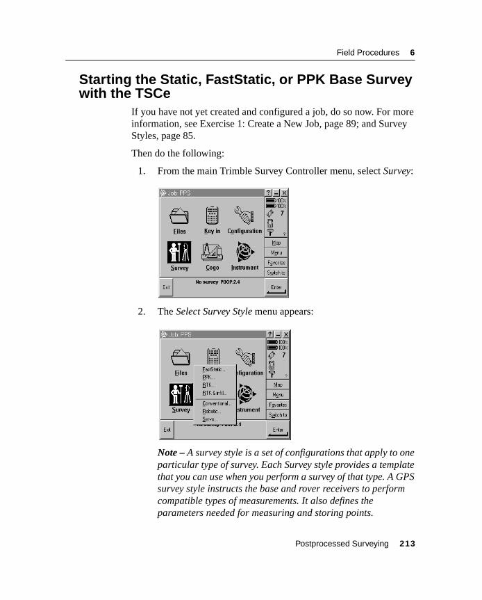
Field Procedures 6
6.3 Starting the Static, FastStatic, or PPK Base Survey with the TSCe
If you have not yet created and configured a job, do so now. For more information, see Exercise 1: Create a New Job, page 89; and Survey Styles, page 85.
Then do the following:
1. From the main Trimble Survey Controller menu, select Survey:
2. The Select Survey Style menu appears:
Note – A survey style is a set of configurations that apply to one particular type of survey. Each Survey style provides a template that you can use when you perform a survey of that type. A GPS survey style instructs the base and rover receivers to perform compatible types of measurements. It also defines the parameters needed for measuring and storing points.
Postprocessed Surveying 213
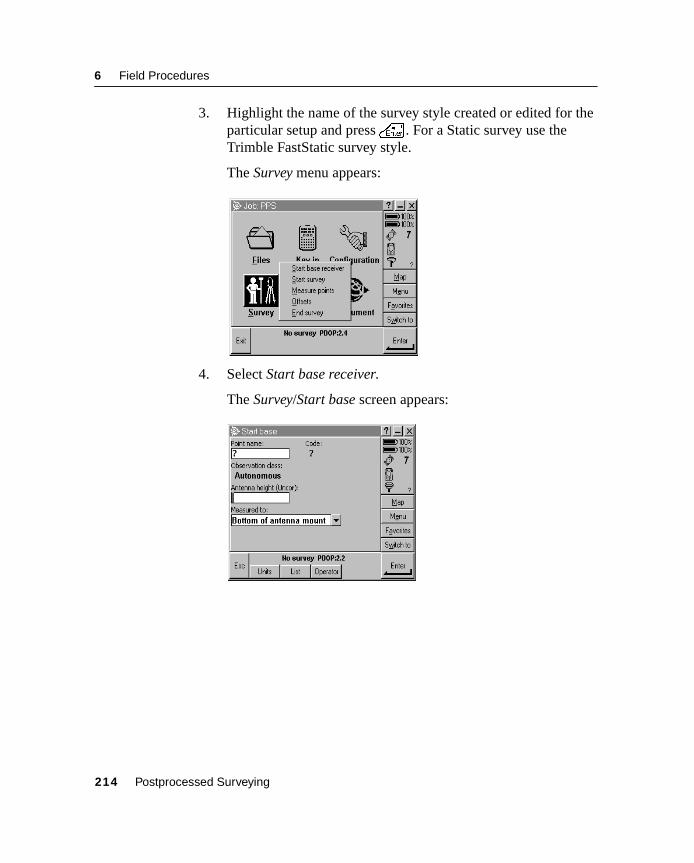
6 Field Procedures
3. Highlight the name of the survey style created or edited for the particular setup and press \ . For a Static survey use the Trimble FastStatic survey style.
The Survey menu appears:
4. Select Start base receiver.
The Survey/Start base screen appears:
214 Postprocessed Surveying
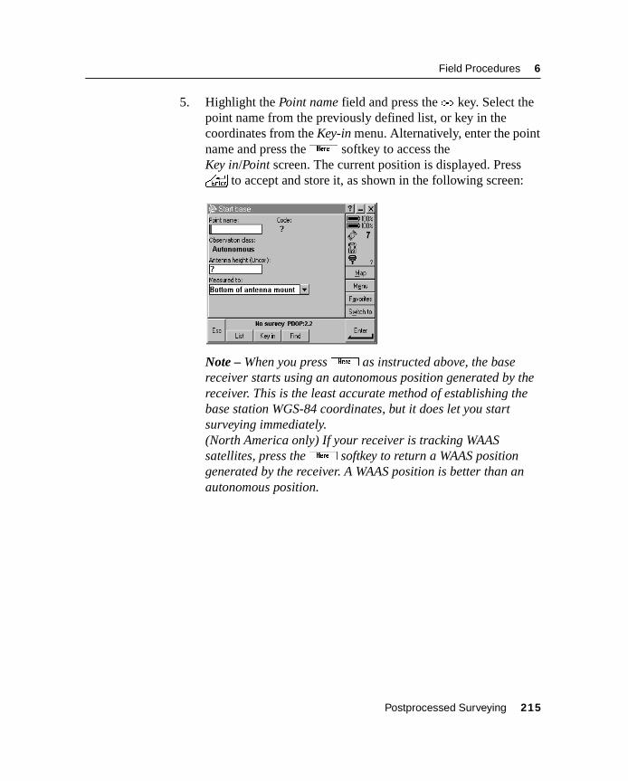
Field Procedures 6
5. Highlight the Point name field and press the ( key. Select the point name from the previously defined list, or key in the coordinates from the Key-in menu. Alternatively, enter the point name and press the ) softkey to access the Key in/Point screen. The current position is displayed. Press \ to accept and store it, as shown in the following screen:
Note – When you press ) as instructed above, the base receiver starts using an autonomous position generated by the receiver. This is the least accurate method of establishing the base station WGS-84 coordinates, but it does let you start surveying immediately.(North America only) If your receiver is tracking WAAS satellites, press the ) softkey to return a WAAS position generated by the receiver. A WAAS position is better than an autonomous position.
Postprocessed Surveying 215
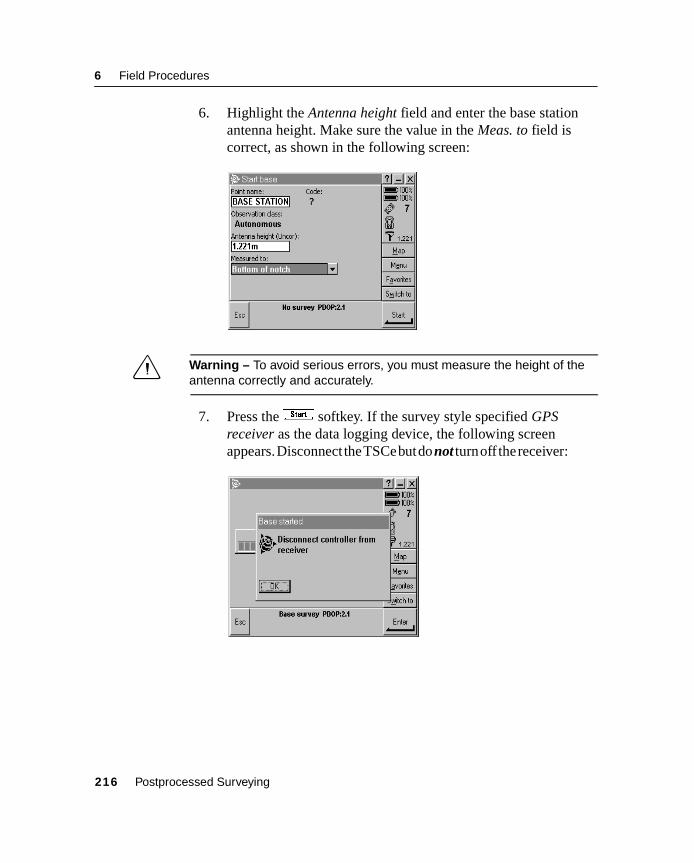
6 Field Procedures
6. Highlight the Antenna height field and enter the base station antenna height. Make sure the value in the Meas. to field is correct, as shown in the following screen:
C Warning – To avoid serious errors, you must measure the height of the antenna correctly and accurately.
7. Press the x softkey. If the survey style specified GPS receiver as the data logging device, the following screen appears. Disconnect the TSCe but do not turn off the receiver:
216 Postprocessed Surveying

Field Procedures 6
Note – If the survey style specified Controller as the data logging device, the following screen appears:
If you specified Controller as a data logging device in your survey style, do not disconnect the TSCe or turn off the receiver.
If you specified Receiver as a data logging device in your survey style, disconnect the TSCe but do not turn off the receiver.
Postprocessed Surveying 217

6 Field Procedures
6.4 Starting the Survey without the TSCeThe following surveys can be started/ended from the receiver front panel. The TSCe is not required:
• Static/FastStatic or PPK base survey
• Static/FastStatic rover survey
Note – PPK rover survey requires TSCe.
When using the 5700 receiver:
• To start the receiver, press the Power button.
• To start or stop logging data, press the Data button. Data is logged onto a Compact Flash Card.
The 5700 receiver automatically assigns a filename and creates a tracking session file when you press the Data button and the receiver begins tracking four or more satellites.
For file naming convention, see Data Management, page 106.
218 Postprocessed Surveying

Field Procedures 6
6.5 Starting the Static/FastStatic Rover SurveyTo start the Static/FastStatic rover survey:
1. From the main menu, select Survey.
2. The Select Survey Style menu appears:
3. Select the Trimble FastStatic Survey Style and press \ .
Postprocessed Surveying 219
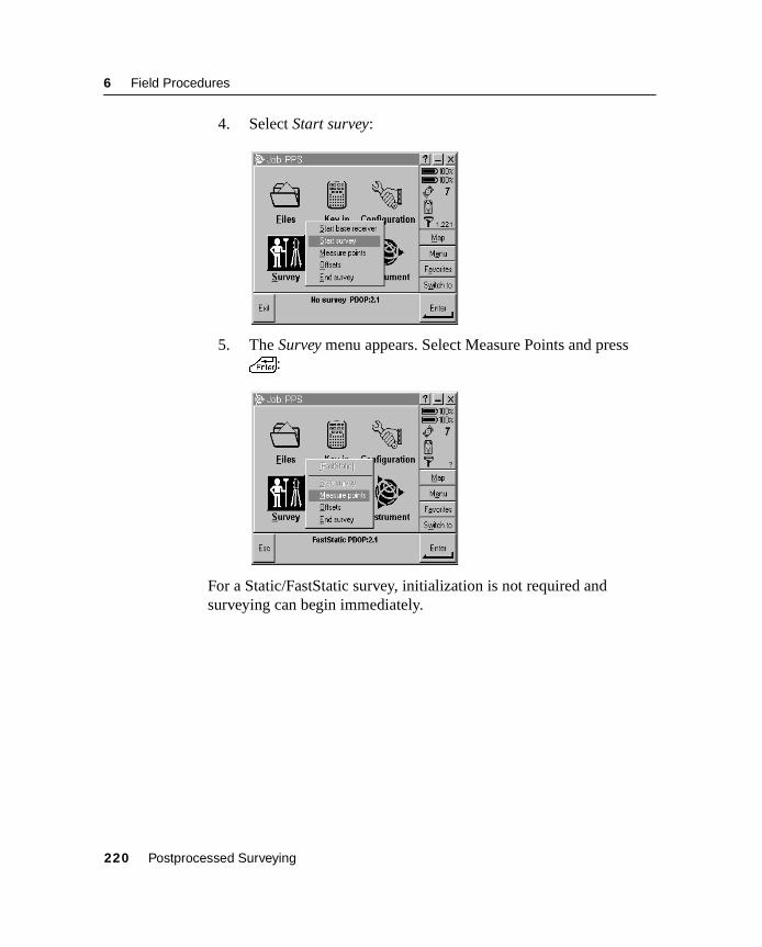
6 Field Procedures
4. Select Start survey:
5. The Survey menu appears. Select Measure Points and press \:
For a Static/FastStatic survey, initialization is not required and surveying can begin immediately.
220 Postprocessed Surveying
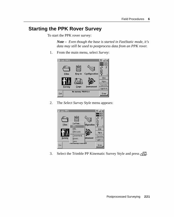
Field Procedures 6
6.6 Starting the PPK Rover SurveyTo start the PPK rover survey:
Note – Even though the base is started in FastStatic mode, it’s data may still be used to postprocess data from an PPK rover.
1. From the main menu, select Survey:
2. The Select Survey Style menu appears:
3. Select the Trimble PP Kinematic Survey Style and press \.
Postprocessed Surveying 221
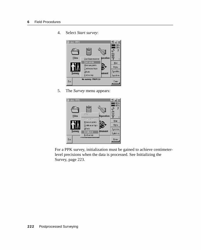
6 Field Procedures
4. Select Start survey:
5. The Survey menu appears:
For a PPK survey, initialization must be gained to achieve centimeter-level precisions when the data is processed. See Initializing the Survey, page 223.
222 Postprocessed Surveying

Field Procedures 6
6.7 Initializing the SurveyWhen performing a PPK survey with a 5700 receiver, the following screen appears when you select Start Survey/Initialization:
Use one of the following methods to initialize dual-frequency PPK surveys in the field:
• On-the-Fly (OTF)
• Known point
• New point
Note – The OTF receiver option is not necessary for postprocessed OTF initializations. With a 5700 receiver, OTF initialization is attempted automatically.
Always collect sufficient raw data when using these methods. Table 6.1 shows the time required to initialize a PPK survey using the various initialization methods.
Table 6.1 Trimble PPK initialization times
Initialization method 4 SVs 5 SVs 6+ SVs
L1/L2 OTF N/A 15 min 8 min
L1/L2 New Point 20 min 15 min 8 min
Known Point at least 4 epochs
Postprocessed Surveying 223
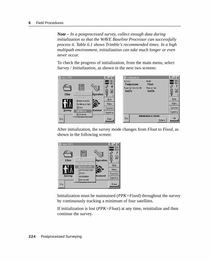
6 Field Procedures
Note – In a postprocessed survey, collect enough data during initialization so that the WAVE Baseline Processor can successfully process it. Table 6.1 shows Trimble’s recommended times. In a high multipath environment, initialization can take much longer or even never occur.
To check the progress of initialization, from the main menu, select Survey / Initialization, as shown in the next two screens:
After initialization, the survey mode changes from Float to Fixed, as shown in the following screen:
Initialization must be maintained (PPK=Fixed) throughout the survey by continuously tracking a minimum of four satellites.
If initialization is lost (PPK=Float) at any time, reinitialize and then continue the survey.
224 Postprocessed Surveying
Field Procedures 6
Note – With 5700 receivers, the initialization process begins automatically if at least five L1/L2 satellites are being observed.
B Tip – If you do an OTF initialization in a postprocessed kinematic survey, you can measure points before initialization is gained. Trimble Geomatics Office can back-process the data later to give a fixed solution. If you do this but lose lock on the satellites while initializing, re-measure any one of the points that you surveyed before lock was lost.
Multipath
Initialization reliability depends on the initialization method used and on whether or not multipath occurred during the initialization phase. (Multipath occurs when GPS signals are reflected off objects such as the ground or a building).
The occurrence of multipath at the GPS antenna adversely affects GPS initializations and solutions:
• If initialization is by the Known Point or Initializer Bar method, multipath can cause an initialization attempt to fail.
• If initialization is by the OTF or New Point method, it is difficult to detect the presence of multipath during the initialization. If there is multipath, the receiver may take a long time to initialize or it may not initialize at all.
Note – If you survey points with a bad initialization, position errors result. To minimize the effect of multipath during an OTF initialization, move around.
Postprocessed Surveying 225
6 Field Procedures
6.7.1 On-the-Fly (OTF) Initialization
OTF initialization is automatic when there are five or more L1/L2 satellites. When the status line shows PPK=Fixed, the receiver has logged an OTF initialization for this block of data. For more information, see the Tip on page 225.
6.7.2 Known Point Initialization
To perform a Known Point initialization:
1. Position the rover antenna over a known point.
2. From the Survey menu, choose Initialization.
3. Set the Method field to Known Point and press \ .
4. Enter a value in the Point name field. (This must be the name of a known point in the Trimble Survey Controller database.) While still in the Point name field, press l . Select the point from the list of known points.
5. Enter values in the Code and Antenna height fields, and make sure that the setting in the Meas. to field is correct.
6. When the antenna is centered and vertical over the point, press x or \ .
The TSCe starts to record data, and the static icon appears in the status line.
Keep the antenna vertical and stationary while data is recorded.
7. When the receiver is initialized, the results are displayed and the w softkey appears. Press it to accept the initialization.
8. If the initialization fails, the results are displayed. Trimble Survey Controller asks if you want to retry. Press y or z .
226 Postprocessed Surveying

Field Procedures 6
6.7.3 New Point Initialization (No OTF)
To perform a New Point initialization:
1. Position the rover antenna a distance away from the base receiver.
B Tip – Trimble recommends that you use a bipod attached to the range pole when using this method.
2. From the Survey menu, choose Initialization.
3. In the Method field, select New point and then press \.
4. Enter values for the Point name, Code, and Antenna height fields.
5. When the antenna is centered and vertical over the point, press x or \.
The data collector starts to record data, and the static icon appears in the status line.
Keep the antenna vertical and stationary while data is recorded.
6. When the receiver has initialized, the w softkey appears. Press it to store the point.
Postprocessed Surveying 227

6 Field Procedures
6.8 Measuring PointsIn a conventional survey, you can only measure two types of points: topo or check. In a GPS survey, you measure points by choosing one of several predefined point types.
In a GPS survey, the Survey Style (and so the survey type) you choose determines the type of point(s) that can be measured. A single Survey Style cannot measure every kind of point, so you must use different Survey Styles to measure different kinds of point.
A FastStatic Survey Style, for example, can be used to measure FastStatic points only.
A PP Kinematic Style, for example, can be used to measure topo and observed control points.
This section shows how to measure points, Static/FastStatic and PPK methods.
Note – For PPK surveys, initialize the survey before measuring points.
228 Postprocessed Surveying

Field Procedures 6
6.8.1 Measuring a Point in Static/FastStatic Survey
Start survey with FastStatic survey style. For more information, see Starting the Static/FastStatic Rover Survey, page 219.
To measure a point:
1. From the main menu, select Survey / Measure points.
2. Enter values in the Point name and Code fields (the latter is optional). The Type field is set to FastStatic point.
3. Enter a value in the Antenna height field and make sure that the setting in the Meas to. field is correct.
4. When the antenna is vertical and stationary, press \ or m to start recording data.
The static icon appears in the status line.
Postprocessed Surveying 229

6 Field Procedures
5. The q softkey appears when the preset occupation time and precisions have been reached. Press it to store the point.
B Tip – In the Survey Style, set the Auto store point field to Yes to automatically store the point when the preset occupation time and precisions have been met.
230 Postprocessed Surveying

Field Procedures 6
6.8.2 Measuring a Point in a PPK Survey
Start survey with PP Kinematic survey style. For more information, see Starting the PPK Rover Survey, page 221.
To measure a point:
1. From the main menu, select Survey. The following screens appear:
2. Postprocessed OTF initialization begins automatically. If you wish to initialize the survey using other available methods, select Initialization / I. The following screen appears:
3. From Survey / Measure Points screen, enter values in the Point name and Code fields (the latter is optional). The Type field is set to Topo point.
4. Enter a value in the Antenna height field and make sure that the setting in the Meas to. field is correct.
Postprocessed Surveying 231

6 Field Procedures
5. When the antenna is vertical and stationary, press \ or m to start recording data.
The static icon appears in the status line.
6. The q softkey appears when the preset occupation time and precisions have been reached. Press it to store the point.
B Tip – In the Survey Style, set the Auto store point field to Yes to automatically store the point when the preset occupation time and precisions have been met.
6.8.3 Measuring Continuous Topo Points
Continuous topo points are stored automatically and continuously after a preset time.
In a postprocessed survey, Trimble Survey Controller can measure a line of continuous topo points.
232 Postprocessed Surveying
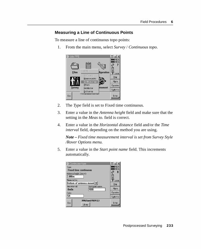
Field Procedures 6
Measuring a Line of Continuous Points
To measure a line of continuous topo points:
1. From the main menu, select Survey / Continuous topo.
2. The Type field is set to Fixed time continuous.
3. Enter a value in the Antenna height field and make sure that the setting in the Meas to. field is correct.
4. Enter a value in the Horizontal distance field and/or the Time interval field, depending on the method you are using.
Note – Fixed time measurement interval is set from Survey Style /Rover Options menu.
5. Enter a value in the Start point name field. This increments automatically.
Postprocessed Surveying 233

6 Field Procedures
6. Press m to start recording data, and then move along the feature to be surveyed.
The TSCe beeps every time a point is recorded.
7. To stop measuring continuous points, press e .
234 Postprocessed Surveying

Field Procedures 6
6.9 Review Questions
1. What is the main advantage of PPK over Static/FastStatic survey methods?
2. Which initialization method is the quickest and most reliable?
3. List the minimum observation times for each initialization method.
4. List three requirements for using the Known Point initialization method.
5. What point types can be observed during Static/FastStatic survey?
6. What point types can be observed during PPK survey?
Initialization method 4 SVs 5 SVs 6+ SVs
L1/L2 OTF
L1/L2 New Point
Known Point
Postprocessed Surveying 235
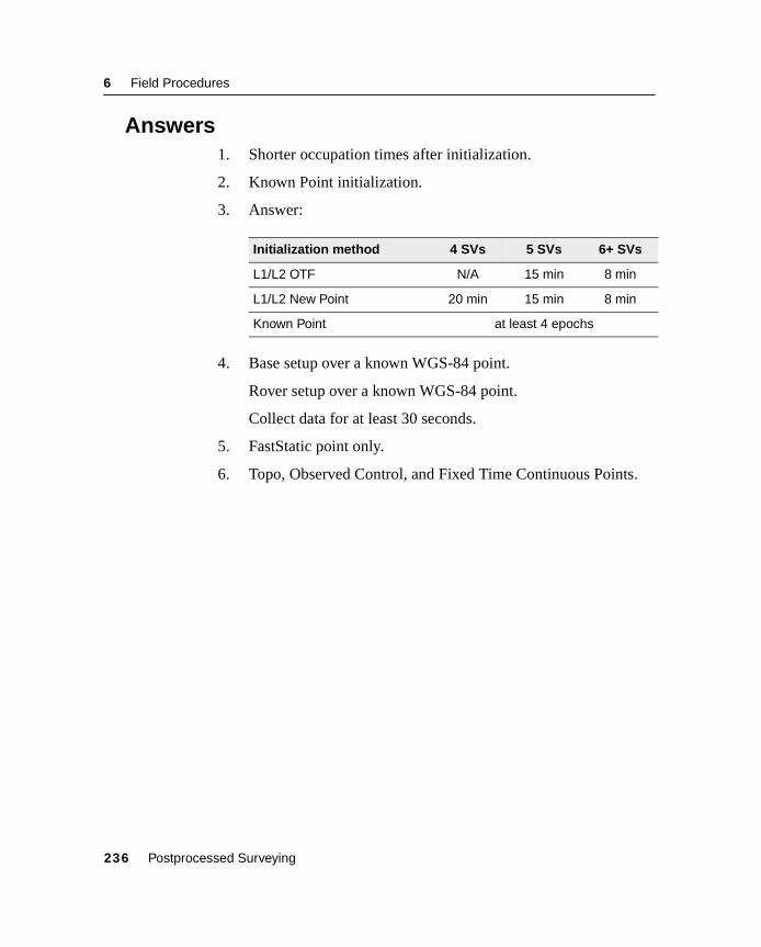
6 Field Procedures
6.10 Answers1. Shorter occupation times after initialization.
2. Known Point initialization.
3. Answer:
4. Base setup over a known WGS-84 point.
Rover setup over a known WGS-84 point.
Collect data for at least 30 seconds.
5. FastStatic point only.
6. Topo, Observed Control, and Fixed Time Continuous Points.
Initialization method 4 SVs 5 SVs 6+ SVs
L1/L2 OTF N/A 15 min 8 min
L1/L2 New Point 20 min 15 min 8 min
Known Point at least 4 epochs
236 Postprocessed Surveying

C H A P T E R
7
Office Procedures 7In this chapter:
■ Introduction
■ Session objectives
■ Transferring field data
■ Baseline processing
■ A guide to least-squares adjustment
■ Network adjustment

7 Office Procedures
7.1 IntroductionThis chapter describes how to use the following Trimble Geomatics Office modules:
• WAVE (Weighted Ambiguity Vector Estimator) Baseline Processor
This module provides all the tools required to process raw GPS data collected using Static/FastStatic or PP Kinematic survey techniques.
• Network Adjustment
This module provides all the tools required to perform a complete network adjustment.
Sample data provided with Trimble Geomatics Office are used as a tutorial for:
• Creating a project using the sample data template
• Importing sample data files
• Processing GPS baselines
• Adjusting a network using GPS and terrestrial observations.
238 Postprocessed Surveying

Office Procedures 7
7.2 Session ObjectivesBy the end of this session you will be able to use:
• The Trimble Geomatics Office software to:
– Import data from the field session
• The WAVE Baseline Processor module to:
– Edit occupations and input coordinate seed
– Set the display and processing style
– Select baselines for processing
– Process baselines
– Evaluate the results of baseline processing
• The Network Adjustment module to:
– Select processed GPS baselines to use in the network adjustment
– Perform the minimally constrained GPS network adjustment
– Import terrestrial observations
– Perform the minimally constrained terrestrial network adjustment
– Load the geoid
– Scale the geoid
– Perform a fully constrained network adjustment
– Evaluate the results of the adjustment
Postprocessed Surveying 239
7 Office Procedures
7.3 Transferring Field DataDepending on the choice of the equipment and settings in your survey style, data collected during a field session can be stored in Trimble Survey Controller or GPS receiver CompactFlash card/internal memory.
Transfer raw GPS data collected in the field into the Trimble Geomatics Office software database.
Note – Raw GPS observations are stored inside the TSCe memory, receiver’s internal memory, or CompactFlash card in a special compressed format. The TSCe uses .RAW format and the 5700 GPS receiver uses the T00 format. Once these files are transferred to the PC they are automatically converted to .DAT format. You only see the file extensions for the 5700 receiver.
To process GPS baselines and adjust the network, use one of the following methods to transfer the data to the PC and then to a Trimble Geomatics Office project database.
1. Import data directly from the survey device to the Trimble Geomatics Office project database.
2. Use Data Transfer to transfer files to your PC. Use the Import function to import files to a Trimble Geomatics Office project database.
240 Postprocessed Surveying
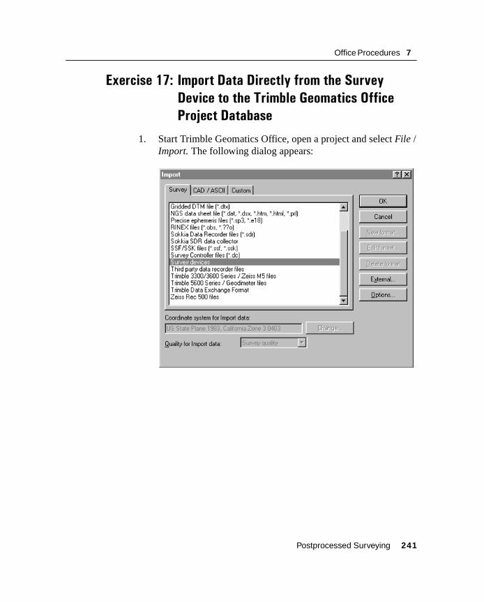
Office Procedures 7
Exercise 17: Import Data Directly from the Survey
Device to the Trimble Geomatics Office
Project Database
1. Start Trimble Geomatics Office, open a project and select File / Import. The following dialog appears:
Postprocessed Surveying 241
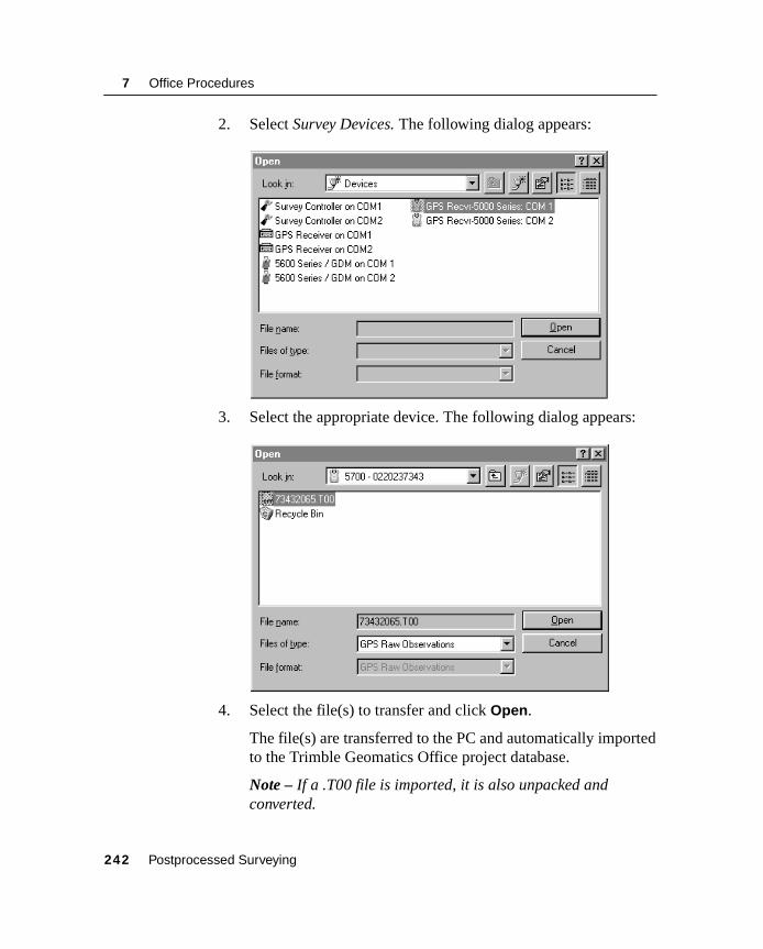
7 Office Procedures
2. Select Survey Devices. The following dialog appears:
3. Select the appropriate device. The following dialog appears:
4. Select the file(s) to transfer and click Open.
The file(s) are transferred to the PC and automatically imported to the Trimble Geomatics Office project database.
Note – If a .T00 file is imported, it is also unpacked and converted.
242 Postprocessed Surveying

Office Procedures 7
Exercise 18: Transfer Files to the PC and Import them
into a Trimble Geomatics Office Project
First, transfer files to the PC, then import them to the Trimble Geomatics Office project database.
The following dialog shows files transferred to a PC from Trimble Survey Controller or the GPS receiver using Data Transfer, and saved to a designated folder:
Postprocessed Surveying 243
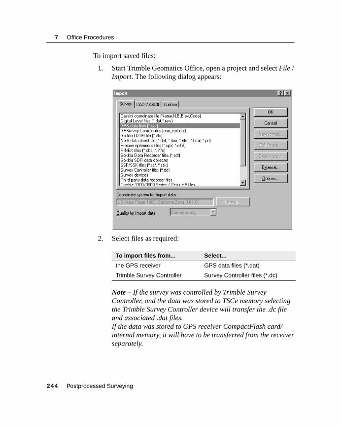
7 Office Procedures
To import saved files:
1. Start Trimble Geomatics Office, open a project and select File / Import. The following dialog appears:
2. Select files as required:
Note – If the survey was controlled by Trimble Survey Controller, and the data was stored to TSCe memory selecting the Trimble Survey Controller device will transfer the .dc file and associated .dat files.If the data was stored to GPS receiver CompactFlash card/internal memory, it will have to be transferred from the receiver separately.
To import files from... Select...
the GPS receiver GPS data files (*.dat)
Trimble Survey Controller Survey Controller files (*.dc)
244 Postprocessed Surveying
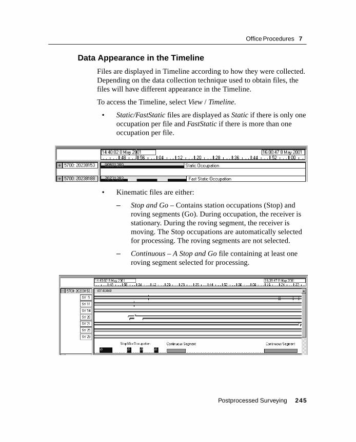
Office Procedures 7
7.3.1 Data Appearance in the Timeline
Files are displayed in Timeline according to how they were collected. Depending on the data collection technique used to obtain files, the files will have different appearance in the Timeline.
To access the Timeline, select View / Timeline.
• Static/FastStatic files are displayed as Static if there is only one occupation per file and FastStatic if there is more than one occupation per file.
• Kinematic files are either:
– Stop and Go – Contains station occupations (Stop) and roving segments (Go). During occupation, the receiver is stationary. During the roving segment, the receiver is moving. The Stop occupations are automatically selected for processing. The roving segments are not selected.
– Continuous – A Stop and Go file containing at least one roving segment selected for processing.
Postprocessed Surveying 245

7 Office Procedures
246 Postprocessed Surveying

Office Procedures 7
7.4Baseline Processing
In this section:
■ Baseline processing theory
■ GPS processing style
■ Processing baselines
■ Reviewing baseline solutions
■ Loop closures
■ Troubleshooting problem data sets
■ Baseline processing review questions
■ Creating a project using the sample data template
■ Importing sample data files
■ Importing control coordinates
■ Processing GPS baselines
■ GPS Loop closures
Postprocessed Surveying 247

7 Office Procedures
248 Postprocessed Surveying
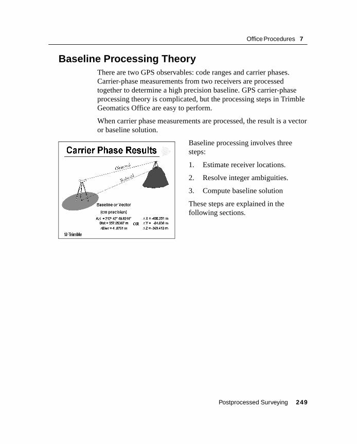
Office Procedures 7
7.5 Baseline Processing TheoryThere are two GPS observables: code ranges and carrier phases. Carrier-phase measurements from two receivers are processed together to determine a high precision baseline. GPS carrier-phase processing theory is complicated, but the processing steps in Trimble Geomatics Office are easy to perform.
When carrier phase measurements are processed, the result is a vector or baseline solution.
Baseline processing involves three steps:
1. Estimate receiver locations.
2. Resolve integer ambiguities.
3. Compute baseline solution
These steps are explained in the following sections.
Postprocessed Surveying 249

7 Office Procedures
7.5.1 Estimating receiver location
Before processing begins, the WAVE baseline processor needs an approximate position of the receiver. WAVE gets this position from code positions or by coordinate seeding.
Use the position obtained by code range measurements as the approximate initial position.
This range is based on the equation:
Distance = Velocity × Time
The signal travels at the speed of light. The receiver determines travel time from the modulated code, then calculates the range to the SV. As long as the ranges to at least four SVs are known, a resection will determine the position of the APC.
The code position is usually good enough for an approximate position. Keep in mind that C/A code based (autonomous) position is accurate to 15–20 m. These positioning errors can introduce other errors into the baseline solution.
Coordinate seeding
Processing with an accurate WGS-84 position, either L,L,h or X,Y,Z is called coordinate seeding. You can enter coordinates into the software by:
• Importing an ASCII file of the known coordinates
• Editing the true coordinates for points using the Properties window
To provide seeding to a project, confirm the point qualities of the seeded points are set to Control Quality.
Receiver Location
D
Distance D = Speed of Light x Time
Code Position
250 Postprocessed Surveying
Office Procedures 7
WAVE computes other station positions relative to a reference station. When a baseline is computed between two stations, one is held fixed as a reference. The coordinate may consist of latitude, longitude, and/or ellipsoid height in reference to the WGS-84 ellipsoid.
For every 10 m of error in the reference station, there is 1 ppm potential error in the baseline. Inputting the reference position (coordinate seeding) forces the processor to build the network from this reference, eliminating potential error.
Baselines are processed sequentially. The direction of the baseline, which station is used as the base and which is used as the rover, is determined automatically by the processor. The direction is optimized for the transfer of precise coordinates. This transfer of precise control coordinates from one point to another is referred to as coordinate seeding. The baseline processor automatically chooses the highest quality points in the processing session to use as the coordinate seed, and baselines are computed outward from those points.
The processor will use the highest station quality of the selected baselines as the starting point for the direction of processing. These qualities are:
• Control
• Survey
• Mapping
• Unknown
Baseline Flow
In most cases, the processor will select the appropriate direction for processing, particularly if care has been used in setting up control in Trimble Geomatics Office. In some instances it may be desirable to switch the direction of the baseline by swapping the base and rover.
Postprocessed Surveying 251
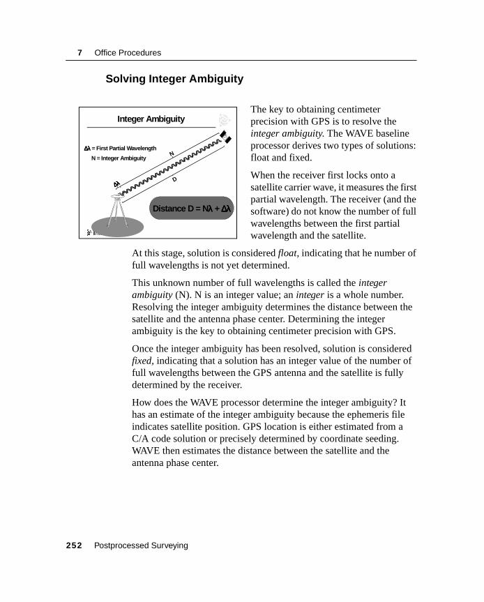
7 Office Procedures
7.5.2 Solving Integer Ambiguity
The key to obtaining centimeter precision with GPS is to resolve the integer ambiguity. The WAVE baseline processor derives two types of solutions: float and fixed.
When the receiver first locks onto a satellite carrier wave, it measures the first partial wavelength. The receiver (and the software) do not know the number of full wavelengths between the first partial wavelength and the satellite.
At this stage, solution is considered float, indicating that he number of full wavelengths is not yet determined.
This unknown number of full wavelengths is called the integer ambiguity (N). N is an integer value; an integer is a whole number. Resolving the integer ambiguity determines the distance between the satellite and the antenna phase center. Determining the integer ambiguity is the key to obtaining centimeter precision with GPS.
Once the integer ambiguity has been resolved, solution is considered fixed, indicating that a solution has an integer value of the number of full wavelengths between the GPS antenna and the satellite is fully determined by the receiver.
How does the WAVE processor determine the integer ambiguity? It has an estimate of the integer ambiguity because the ephemeris file indicates satellite position. GPS location is either estimated from a C/A code solution or precisely determined by coordinate seeding. WAVE then estimates the distance between the satellite and the antenna phase center.
Integer Ambiguity
∆λ∆λ∆λ∆λ
∆λ∆λ∆λ∆λ = First Partial WavelengthN
N = Integer Ambiguity
D
Distance D = Nλλλλ + ∆λ∆λ∆λ∆λ
252 Postprocessed Surveying
Office Procedures 7
Dividing distance by carrier phase wavelength calculates the number of wavelengths. This computation does not produce an integer value. When the processor has only float or decimal values for the integer ambiguity, the processor produces a float solution. The processor starts with the float solution and attempts to determine the correct integer values for the integer ambiguity.
Carrier Phase Differencing
What does the baseline processor do with these phase measurements?
When a signal is transmitted from a satellite, it travels to all operating receivers. The signal to one of the receivers is used as a reference signal. When this reference is compared to the signal received at the other receiver, there is a signal phase difference between the two receivers. Phase differences are derived with all the other satellites in view.
WAVE uses a method called differencing. For each ambiguity, WAVE replaces a float or decimal value with the nearest integer. It then recomputes a baseline solution for this integer set and computes a variance factor for every integer combination. The baseline processor can now compute precise distances from the receiver to the satellite to compute the receiver’s precise position.
7.5.3 Baseline Solution
The processor computes precise ranges to the satellites from the receiver once the integer ambiguities are solved. Once receiver positions are known, those positions are inversed to calculate a vector, or baseline, solution. This vector has centimeter precision.
A baseline is the measured vector between the phase centers of two antennas. Set up the antennas carefully, and measure their heights accurately; the software reduces the baseline solution from one survey monument to the other.
Postprocessed Surveying 253
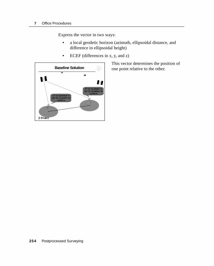
7 Office Procedures
Express the vector in two ways:
• a local geodetic horizon (azimuth, ellipsoidal distance, and difference in ellipsoidal height)
• ECEF (differences in x, y, and z)
This vector determines the position of one point relative to the other.Baseline Solution
37o 23’ 30.195065” N122o 02’ 33.948394” W
-12.445 m37o 23’ 28.607434” N
122o 02’ 41.161474” W-12.637 m
254 Postprocessed Surveying
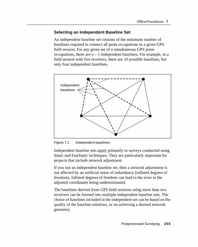
Office Procedures 7
Selecting an Independent Baseline Set
An independent baseline set consists of the minimum number of baselines required to connect all point occupations in a given GPS field session. For any given set of n simultaneous GPS point occupations, there are n – 1 independent baselines. For example, in a field session with five receivers, there are 10 possible baselines, but only four independent baselines.
Figure 7.1 Independent baselines
Independent baseline sets apply primarily to surveys conducted using Static and FastStatic techniques. They are particularly important for projects that include network adjustment.
If you use an independent baseline set, then a network adjustment is not affected by an artificial sense of redundancy (inflated degrees of freedom). Inflated degrees of freedom can lead to the error in the adjusted coordinates being underestimated.
The baselines derived from GPS field sessions using more than two receivers can be formed into multiple independent baseline sets. The choice of baselines included in the independent set can be based on the quality of the baseline solutions, or on achieving a desired network geometry.
Independentbaselines
Postprocessed Surveying 255
7 Office Procedures
To specify an independent baseline set, do one of the following:
• Only process the baselines originally planned during the mission planning stage.
• Select and process only an independent set of baselines from among all potential baselines for a GPS field session.
• Process all potential baselines for a GPS field session and select an independent set at the time the results are saved to the project.
• Process all potential baselines for a GPS field session and save all the results to the project, then specify that the dependent baselines are not considered in a network adjustment.
You can use the Dependent Baseline View tool to link the observations in the graphics window and Timeline. When you select this tool, the software only shows postprocessed baselines in the current Timeline view, and the postprocessed baselines that were observed at the same time. All other postprocessed baselines in the Survey view are hidden.
Use this tool to show baselines that were observed at the same time and then prevent the dependent baselines from being considered in an adjustment. The best way to prevent baselines from being considered is to use the Multiple Edit dialog.
For example, to change the status of dependent baselines to disabled:
1. Select the Dependent baseline view tool.
2. Select the dependent baselines in the graphics window.
3. Select Edit / Multiple Edit. The Multiple Edit dialog appears.
4. In the Survey tab, select the Set observation status to check box.
5. From the list, select Disabled and then click OK.
The selected observations will now have a disabled status.
256 Postprocessed Surveying

Office Procedures 7
You can also prevent baselines from being used by performing one of the following operations in the Properties window:
• Change the status of the dependent baselines to disabled.
• Change the status of the dependent baselines to enabled as check.
• Clear the Use in Network Adjustment check box for the dependent baselines.
Alternatively:
• In the Observations dialog, clear the Use check box for the dependent baselines.
Once the survey style has been configured and applied, independent baselines selected, you can proceed with processing baselines.
7.6 GPS Processing StyleGPS processing styles let you customize your processing for specific requirements, such as processing with precise ephemeris or a specific elevation mask. The settings can be saved as a style and recalled at a later time simply by specifying the name of that style. You can develop a processing style library to work with common processing scenarios.
To specify the active style:
1. Select Survey / GPS Processing Styles. The GPS Processing Styles dialog appears.
2. Click on the desired style. This style then becomes the active style.
3. Click OK to accept this style or Cancel to exit without making any changes.
Postprocessed Surveying 257

7 Office Procedures
Exercise 19: Create and Configure a GPS Processing
Style
You can create and configure baseline processing styles at any time. You can save changes to a baseline processing style with a descriptive name, and use that style as the active style in future processing sessions.
To create a new baseline processing styles using common processing controls:
From the GPS Processing Styles dialog, click:
– Edit to define style controls
– New to create a new style using Trimble default settings
– Copy to create a new style based on an existing style
– Rename to change the name of the active style
– Delete to remove the active style
258 Postprocessed Surveying

Office Procedures 7
1. From the Survey menu, choose GPS Baseline Processing Styles. The GPS Processing Styles dialog appears with the available styles listed in alphabetical order. The active style is highlighted, as shown below:
2. Click Copy or New.
B Tip – The copy function makes a copy of the style you have selected and lets you edit the copy of that style. Clicking New initializes a new style with the Trimble Geomatics Office software defaults. It is often easier to create a new style by copying an existing style that is close to the style you want to create.
In this example the Copy Style dialog appears with Copy of Trimble Default in the Name field. Typically this name is changed to something more meaningful, such as Precise Ephemeris Controls.
Postprocessed Surveying 259

7 Office Procedures
3. Click OK. A dialog appears with the name of the new style in the title bar. The most common processing controls—elevation mask, ephemeris type, and final solution type—are available for editing from this dialog.
Use the following:
– Elevation mask – to raise or lower the elevation mask.
– Ephemeris – to change the ephemeris used in processing from Broadcast to Precise.
– Solution type – to change the final baseline processor solution to Code, Float, or Fixed.
260 Postprocessed Surveying

Office Procedures 7
For more settings click Advanced from the processing style dialog. The following dialog appears:
This dialog has eight tabs:
4. Click OK to save style changes and return to the GPS Processing Styles dialog.
Tab Use it to...
Static control Static and FastStatic baseline processing.
Kinematic control Kinematic baseline processing.
Global control Static and Kinematic processing.
Quality identify and remove marginal data and solutions while processing and before saving the processing results to the project. Also use it to determine which solutions pass, are flagged, or fail.
Tropo select and apply tropospheric models.
Iono apply ionospheric modeling.
Events interpolate and display events.
OTF Search control on-the-fly initialization strategies.
Postprocessed Surveying 261

7 Office Procedures
7.7 Processing BaselinesStart the processor using one of the following methods:
• From the Survey menu, select Process GPS Baselines.
• From the Trimble Survey group in the project bar, click the Process GPS Baselines shortcut.
• From the Process group in the project bar, click the Process GPS Baselines shortcut.
The GPS Processing dialog appears.
262 Postprocessed Surveying

Office Procedures 7
7.8 Reviewing Baseline SolutionsAfter processing baselines, a summary of each baseline solution is displayed.
The solution summary contains:
• ID
• From and To stations
• Baseline length
• Solution Type
• Ratio
• Reference Variance
• RMS
Postprocessed Surveying 263

7 Office Procedures
Solution Types
The processor tries various processing combinations to produce the highest possible quality baseline solution. If the processing fails the criteria of the Processing Style, the Use column will appear unchecked. If left unchecked, its contents will not be used to update the network.
Baseline solution types:
• Fixed – indicates that the baseline processor solved the integer ambiguities.
• Float – indicates that the baseline processor did not find a set of integers statistically better than any other set of integers.
The key to centimeter precision with GPS is the ability to resolve the integer ambiguities.
L1 Only
WAVE computes an L1 solution from single-frequency receivers; it also computes an L1 solution for baselines less than 5 km from dual-frequency receivers. For dual-frequency data, L2 is used to help resolve the integer ambiguities.
Iono-Free
An iono-free solution uses data from both L1 and L2 signals. WAVE uses both frequencies to correct errors introduced by the ionosphere in baselines longer than 5 km. The L2 signal from the dual-frequency receiver is used by the processor to determine the integer ambiguities.
Float
Sometimes, especially for long baselines, a float solution is the best WAVE can compute. A float solution does not necessarily mean that the baseline solution is invalid. A float solution indicates a problem for baselines less than 5 km. For longer baselines, evaluate the baseline quality by checking the reference variance, RMS, and residual plots.
264 Postprocessed Surveying

Office Procedures 7
Reference Variance
The reference variance is a unitless number indicating how well the observed data for a baseline fit the computed solution. The processor estimates error before processing. After processing, it looks at the actual error, the residuals, in the solution. The processor compares the actual error to its estimated error. When the reference variance approximates 1.00, the solution is statistically sound.
Ratio
The ratio is the relationship between the variance of the second-best candidate fixed solution to the variance of the best-candidate fixed solution generated by the processor’s integer search. Higher ratios indicate larger differences between the variance of the best choice and the second-best choice. WAVE only considers a solution fixed if the ratio is greater than 1.5. Only fixed-integer solutions have ratios, and high ratios are desired.
Ratios are GPS data quality indicators, not human error indicators.
View the ratios and reference variances together. Check baselines with low ratios and high reference variances.
RMS
Another statistic that allows you to evaluate the quality of the baseline solution is the root mean square (RMS). The baseline solution is an estimate using all of the data collected in the field. The WAVE processor compares each measurement epoch to the baseline solution. Each epoch is then compared, and the differences averaged.
The RMS is the average of the epochs’ residuals. Values less than 15 mm are acceptable for most small to medium-sized projects.
Detailed Solution Report
The Detailed Report displays the following information about an individual baseline solution:
Postprocessed Surveying 265

7 Office Procedures
• Station information (ID)• Baseline solution error estimates• Ratio, reference variance, RMS• Processor controls • Satellite tracking summaries• Residual plots
To review the report:
1. Highlight the desired baseline, from GPS Processing dialog:
266 Postprocessed Surveying

Office Procedures 7
2. Select Report and the following dialog appears:
3. Copy or print the report if necessary.
Postprocessed Surveying 267

7 Office Procedures
Satellite Tracking Summaries
Tracking summaries indicate the quality of the L1 and L2 signals received from each satellite using a timeline.
As shown in Figure 7.2, a solid line indicates a clean signal. A gap or break in the line indicates a cycle slip or loss of signal. Tick marks indicate when the receiver picked up the satellite signal after a cycle slip. A reference satellite with the highest elevation and cleanest signal is chosen to compute the integer ambiguities and used to display residual plots.
Figure 7.2 Satellite phase tracking summary
268 Postprocessed Surveying

Office Procedures 7
Residual Plots
The residual plots show the RMS of each satellite in the baseline solution. When WAVE computes a baseline, it uses a mathematical process called differencing to solve the integer ambiguities. One differencing method is the double difference. The WAVE processor shows the double difference residuals for all satellites used to calculate the baseline solution.
The x-axis represents the reference SV. The y-axis represents the L1 phase signal measured in meters. The amount a signal varies from the reference signal is called a residual. Residuals centered around zero within a range of ±15 mm indicate a good satellite signal. Like the tracking summary, the residual plot is a useful data quality diagnostic tool. See Figure 7.3.
Figure 7.3 Residual plot
Postprocessed Surveying 269
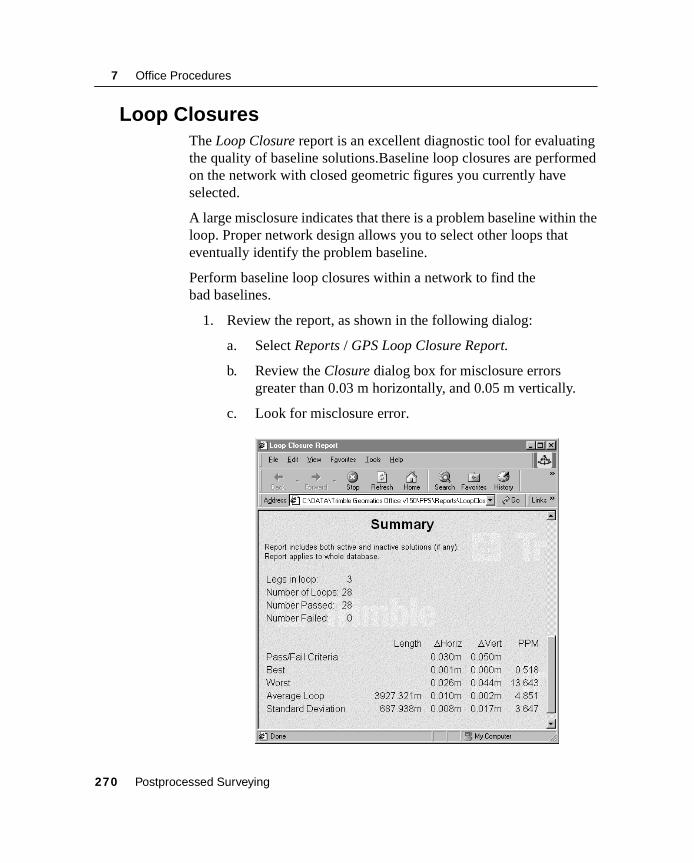
7 Office Procedures
7.9 Loop ClosuresThe Loop Closure report is an excellent diagnostic tool for evaluating the quality of baseline solutions.Baseline loop closures are performed on the network with closed geometric figures you currently have selected.
A large misclosure indicates that there is a problem baseline within the loop. Proper network design allows you to select other loops that eventually identify the problem baseline.
Perform baseline loop closures within a network to find the bad baselines.
1. Review the report, as shown in the following dialog:
a. Select Reports / GPS Loop Closure Report.
b. Review the Closure dialog box for misclosure errors greater than 0.03 m horizontally, and 0.05 m vertically.
c. Look for misclosure error.
270 Postprocessed Surveying
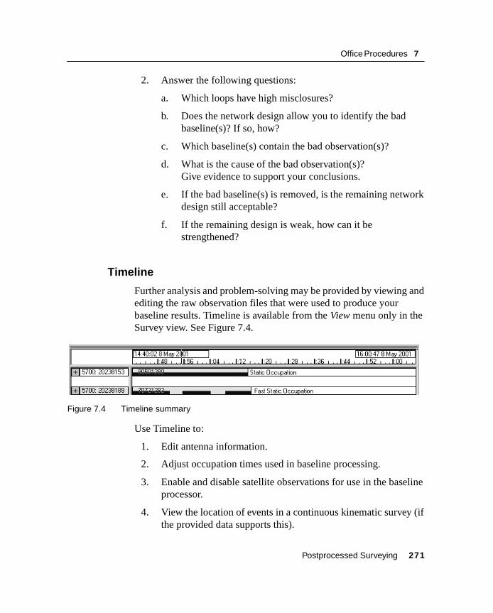
Office Procedures 7
2. Answer the following questions:
a. Which loops have high misclosures?
b. Does the network design allow you to identify the bad baseline(s)? If so, how?
c. Which baseline(s) contain the bad observation(s)?
d. What is the cause of the bad observation(s)? Give evidence to support your conclusions.
e. If the bad baseline(s) is removed, is the remaining network design still acceptable?
f. If the remaining design is weak, how can it be strengthened?
7.9.1 Timeline
Further analysis and problem-solving may be provided by viewing and editing the raw observation files that were used to produce your baseline results. Timeline is available from the View menu only in the Survey view. See Figure 7.4.
Figure 7.4 Timeline summary
Use Timeline to:
1. Edit antenna information.
2. Adjust occupation times used in baseline processing.
3. Enable and disable satellite observations for use in the baseline processor.
4. View the location of events in a continuous kinematic survey (if the provided data supports this).
Postprocessed Surveying 271

7 Office Procedures
5. Create plots for satellite observations.
6. View satellite health and other orbit information.
7.10 Troubleshooting Problem Data SetsSeveral indicators aid in evaluating a GPS solution. Because there are many factors that influence the quality of a baseline solution, it is possible for WAVE to compute a bad solution. In some cases, it is possible to improve the baseline solution with troubleshooting techniques, but troubleshooting does not guarantee better results.
7.10.1 Results Analysis
WAVE provides statistics to evaluate the quality of a baseline solution. These statistics indicate good baselines:
• Reference Variance ~ 1
• ratio > 1.5
• RMS < 15 mm
• residual plots ±15 mm
Using baseline loop closures and performing a network adjustment for more evidence about solution quality.
A network adjustment is the best judge of baseline solution quality. It uses statistical theory and least squares principles to show how well all baselines in a network fit together.
272 Postprocessed Surveying

Office Procedures 7
7.10.2 Good Results
Figure 7.5 shows a satellite tracking summary and residual plot for a satisfactory survey.
Figure 7.5 Satellite tracking summary and residual plot
This solution has ideal values for the reference variance, ratio, and RMS. The tracking summary shows a continuous signal throughout the occupation. The residual plot shown is less than 15 mm and centered around zero.
Postprocessed Surveying 273

7 Office Procedures
7.10.3 Troubleshooting Techniques
Before performing more field work, try to minimize problems by troubleshooting and reprocessing baselines.
Troubleshooting may salvage problem data sets. However, good survey practice and proper GPS session planning help avoid problems that require troubleshooting in postprocessing.
Troubleshooting techniques:
• Remove satellites
• Raise elevation mask
• Change session times
When troubleshooting, consider satellite geometry and occupation time.
274 Postprocessed Surveying

Office Procedures 7
Remove Satellites
Remove satellite signal noise by disabling those satellites in Timeline and reprocessing the baseline. Keep in mind the occupation time and number of satellites remaining. Follow static surveying standards:
• 4 SVs = 20 minutes
• 5 SVs = 15 minutes
• 6+ SVs = 8 minutes
Do not disable too many satellites. Exclude one satellite at a time to determine how it affects the baseline solution.
Remove SatellitesFor example, signals are received from seven satellites during a GPS session, but two of those signals are noisy. One is noisy because the satellite is low in the sky. The other is noisy because trees partially block the signal. The noise may affect the baseline solution in WAVE.
Postprocessed Surveying 275

7 Office Procedures
Use Timeline to remove a satellite, as follows:
1. Select View / Timeline. The following dialog appears:
2. Select the receiver node and expand it to display available satellites.
3. Highlight the observation on which you wish to disable a satellite.
4. Select and highlight the satellite vehicle (SV) number you wish to disable.
5. Right-click on the SV and choose Enable / Disable.
276 Postprocessed Surveying
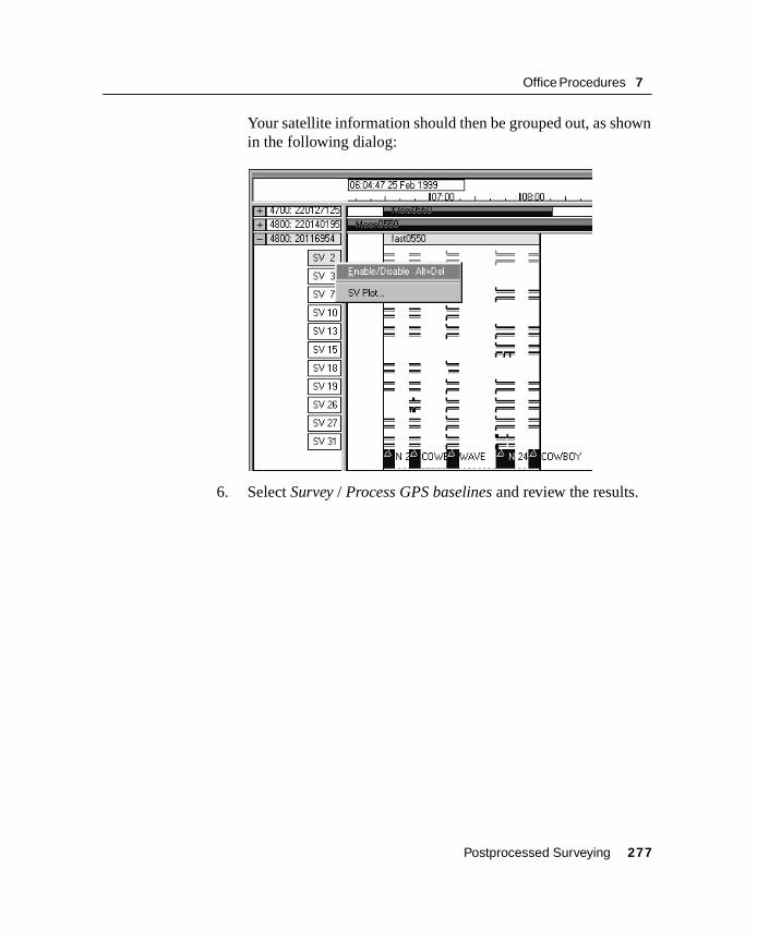
Office Procedures 7
Your satellite information should then be grouped out, as shown in the following dialog:
6. Select Survey / Process GPS baselines and review the results.
Postprocessed Surveying 277

7 Office Procedures
Raise Elevation Mask
Removing a satellite removes all of its signals. Raising the elevation mask preserves the clean signals.
Raising the elevation mask is an easy way to remove noise from a low-elevation satellite. This is useful if the satellite rises higher in the sky and then transmits clean signals. WAVE can use the clean signal in the baseline solution.
To raise the elevation mask:
1. Select Survey / GPS Processing Styles.
2. Edit the survey style. (Alternatively, you can copy an existing style and edit its contents.)
3. In the Basic Processing Styles dialog, type the elevation mask in the Elevation mask (deg) field. (The default is 13 degrees.)
4. Click OK.
5. Select Survey / Process GPS baselines and review the results.
Raise Elevation Mask
15o
18o
20o
If noisy satellites are low in the sky, another way to remove them is to raise the elevation mask in the GPS Processing Style. By raising the elevation mask to 18 degrees, noise from one satellite is removed. Raising the elevation mask even higher would remove the other noisy signal; however, it would also remove a clean signal from another satellite.
278 Postprocessed Surveying
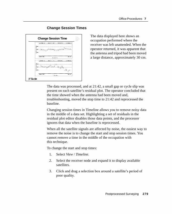
Office Procedures 7
Change Session Times
The data was processed, and at 21:42, a small gap or cycle slip was present on each satellite’s residual plot. The operator concluded that the time showed when the antenna had been moved and, troubleshooting, moved the stop time to 21:42 and reprocessed the baseline.
Changing session times in Timeline allows you to remove noisy data in the middle of a data set. Highlighting a set of residuals in the residual plot editor disables those data points, and the processor ignores that data when the baseline is reprocessed.
When all the satellite signals are affected by noise, the easiest way to remove the noise is to change the start and stop session times. You cannot remove a time in the middle of the occupation with this technique.
To change the start and stop times:
1. Select View / Timeline.
2. Select the receiver node and expand it to display available satellites.
3. Click and drag a selection box around a satellite’s period of poor quality.
Change Session TimeThe data displayed here shows an occupation performed where the receiver was left unattended. When the operator returned, it was apparent that the antenna and tripod had been moved a large distance, approximately 30 cm.
Postprocessed Surveying 279
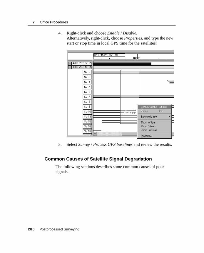
7 Office Procedures
4. Right-click and choose Enable / Disable.Alternatively, right-click, choose Properties, and type the new start or stop time in local GPS time for the satellites:
5. Select Survey / Process GPS baselines and review the results.
7.10.4 Common Causes of Satellite Signal Degradation
The following sections describes some common causes of poor signals.
280 Postprocessed Surveying
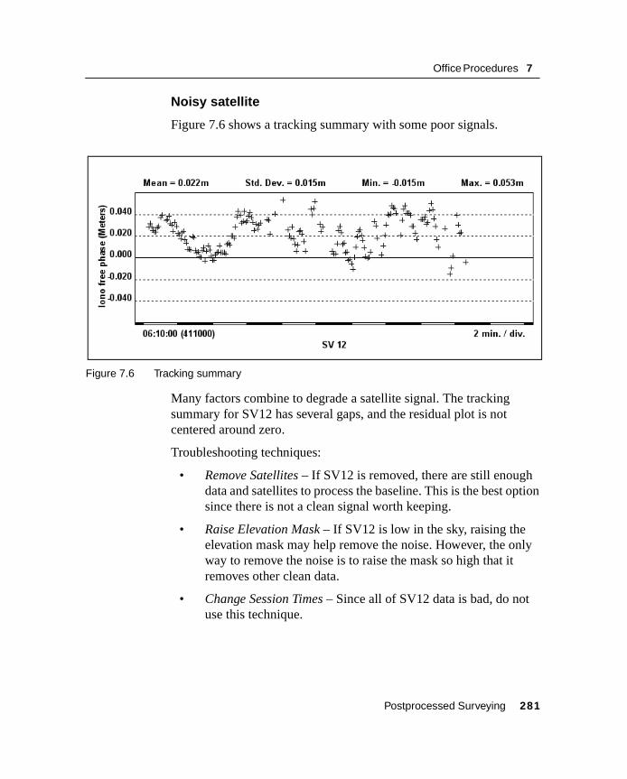
Office Procedures 7
Noisy satellite
Figure 7.6 shows a tracking summary with some poor signals.
Figure 7.6 Tracking summary
Many factors combine to degrade a satellite signal. The tracking summary for SV12 has several gaps, and the residual plot is not centered around zero.
Troubleshooting techniques:
• Remove Satellites – If SV12 is removed, there are still enough data and satellites to process the baseline. This is the best option since there is not a clean signal worth keeping.
• Raise Elevation Mask – If SV12 is low in the sky, raising the elevation mask may help remove the noise. However, the only way to remove the noise is to raise the mask so high that it removes other clean data.
• Change Session Times – Since all of SV12 data is bad, do not use this technique.
Postprocessed Surveying 281

7 Office Procedures
Cycle slips
Figure 7.7 shows a tracking summary with cycle slips.
Figure 7.7 Cycle slips
Cycle slips are common in an urban environment and at times the WAVE processor may resolve some cycle slips improperly.
The combined tracking summary shows a small gap in processed data for several satellites. The residual plots start with a small distribution, but not centered on zero. The jump in the plot coincides with the cycle slip in the combined tracking summary.
If the receiver was tracking the signal, lost it, and then reacquired lock, then the WAVE processor cannot solve the integer ambiguities correctly.
282 Postprocessed Surveying

Office Procedures 7
Troubleshooting techniques:
• Remove Satellites – If cycle slips occurred on only one satellite, remove that satellite from processing. Keep time constraints in mind.
• Raise Elevation Mask – If the noise is due to a low satellite, raising the elevation mask may help.
• Change Session Times – Move the session start time to after the cycle slip occurred, or move the stop time to before the cycle slip occurred. If there is enough data remaining, changing the session times is the best troubleshooting technique.
Incorrect integer ambiguity resolution
Figure 7.8 shows a summary with incorrectly resolved integer ambiguities.
Figure 7.8 Integer ambiguities
The key to centimeter precision with GPS is the ability to resolve integer ambiguities. The WAVE baseline processor may resolve integer ambiguities incorrectly, although this is rare.
Postprocessed Surveying 283
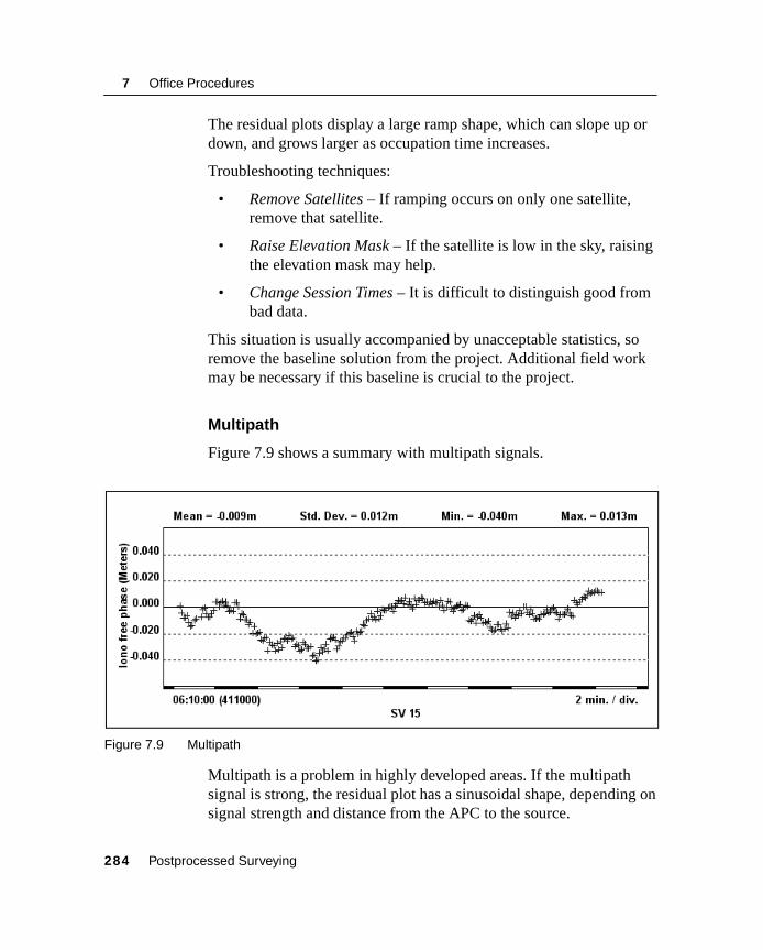
7 Office Procedures
The residual plots display a large ramp shape, which can slope up or down, and grows larger as occupation time increases.
Troubleshooting techniques:
• Remove Satellites – If ramping occurs on only one satellite, remove that satellite.
• Raise Elevation Mask – If the satellite is low in the sky, raising the elevation mask may help.
• Change Session Times – It is difficult to distinguish good from bad data.
This situation is usually accompanied by unacceptable statistics, so remove the baseline solution from the project. Additional field work may be necessary if this baseline is crucial to the project.
Multipath
Figure 7.9 shows a summary with multipath signals.
Figure 7.9 Multipath
Multipath is a problem in highly developed areas. If the multipath signal is strong, the residual plot has a sinusoidal shape, depending on signal strength and distance from the APC to the source.
284 Postprocessed Surveying

Office Procedures 7
There must be enough data to:
• recognize the multipath
• process the baseline after removing the bad data
Troubleshooting techniques:
• Remove Satellite – Remove the affected satellites, leaving enough data to reprocess the baseline.
• Raise Elevation Mask – Multipath is often caused by low satellite elevations. Raising the elevation mask is helpful.
• Change Session Times – If the occupations are long, change session times to exclude the multipath signals.
Try to eliminate multipath sources when planning a GPS project, including using a ground plane or choke ring antenna. If a site is in an environment that is not conducive to GPS, plan long occupation times, which identify multipath in residual plots allowing the WAVE base processor to average the effects out of the solution.
7.10.5 Tips for Troubleshooting Baselines
Troubleshooting problem data sets is similar to processing original baselines. It is useful to work with a printout of the detailed solution summary and view a skyplot of the session time from QuickPlan™ for the problem baseline.
Reprocess the baseline after each troubleshooting change is made.
As you may end up with worse results than the original, reprocess baselines one at a time.
7.10.6 Recompute to Save Changes
When you are satisfied with the results, save the solutions by recomputing the database by Survey / Recompute. Your data should then be ready to be passed through a network adjustment.
Note – Processed baseline solutions can be exported from Trimble Geomatics Office to other third-party network adjustment packages.
Postprocessed Surveying 285

7 Office Procedures
286 Postprocessed Surveying

Office Procedures 7
7.10.7 Baseline Processing Review Questions
1. What two types of signals are measured by the GPS receiver?
2. How do you achieve centimeter precision with GPS?
3. Which datum must be used when inputting a coordinate seed?
4. What are the four station qualities which define the order of coordinate seeding?
5. What is the difference between a float and a fixed solution?
6. What software tools evaluate the quality of a baseline solution?
7. What software tools evaluate the quality of baseline closures on a network.
8. What does a large misclosure indicate?
9. How do you access the Timeline utility?
10. What statistical indicators evaluate baseline solutions?
11. What are the ideal values for those indicators?
12. What do you use the residual plots display for?
13. List three techniques used to troubleshoot problem baselines.
14. What situations do not allow you to utilize troubleshooting techniques?
15. List two things helpful in choosing a troubleshooting technique.
16. How many baselines should you reprocess at one time?
17. How does WAVE know which baselines to apply the selected troubleshooting techniques to?
18. What is the significance of saving a reprocessed baseline solution?
Postprocessed Surveying 287

7 Office Procedures
7.10.8 Baseline Processing Answers
1. Code ranges, carrier-phase
2. By measuring carrier phase observables and solving integer ambiguities.
3. WGS-84.
4. Control, survey, mapping, and unknown.
5. Fixed solution: WAVE solved the integer ambiguity; Float solution: WAVE didn’t find a set of integers statistically better than any other set of integers.
6. GPS Processing dialog, GPS Baseline Processing report.
7. Loop Closure Report.
8. A problem baseline within the loop.
9. Use the View / Timeline option.
10. RMS, reference variance, ratio, residual plots
11. Reference variance ~ 1; Ratio > 1.5; RMS < 15 mm;
Residual plots ±15 mm
12. RMS of each SV compared to the reference SV used to determine a baseline solution.
13. Remove satellites, raise elevation mask, change session times
14. Short occupation times and poor satellite geometry.
15. Occupation time and the number of satellites available.
16. One.
17. Select the baseline to reprocess after troubleshooting. Only selected baselines will be processed.
18. Improving the baseline solution statistics.
288 Postprocessed Surveying

Office Procedures 7
Exercise 20: Processing GPS Baselines
The GPS survey was undertaken by the Survey Crew A with the purpose of establishing a new control point (KTOM).
The specifications for this exercise are:
• Information about existing control was obtained from two sources:
– Published NGS data sheet for points MOON 2 and N 245
– Coordinates for points WAVE and COWBOY are result of previous surveys
• The survey was carried out using four Trimble GPS receivers and three TSCe data collectors.
• A combination of Static and FastStatic field techniques was used.
• All field data have been transferred to the PC.
Your task is to:
• Create a Trimble Geomatics Office project using the Sample Data template
• Import data into the project
• Process GPS baselines
• Perform GPS loop closures
Postprocessed Surveying 289

7 Office Procedures
7.11 Creating a Project Using the Sample Data TemplateTo start the Trimble Geomatics Office software, click and then select Trimble Geomatics Office from the Programs submenu.
To create a project:
1. Do one of the following:
– Select File / New Project.
– In the standard toolbar, select the New Project tool.
– In the project bar, click the New Project shortcut.
2. In the Name field, enter a name for the project.
3. From the Template list, select the Sample Data option.
4. In the New group, make sure that the Project option is selected and then click OK.
The project is created and the Project Properties dialog appears. The values in the fields in each tab are derived from the sample data template.
5. To close the Project Properties dialog, click OK.
290 Postprocessed Surveying
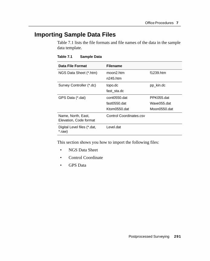
Office Procedures 7
7.12 Importing Sample Data FilesTable 7.1 lists the file formats and file names of the data in the sample data template.
This section shows you how to import the following files:
• NGS Data Sheet
• Control Coordinate
• GPS Data
Table 7.1 Sample Data
Data File Format Filename
NGS Data Sheet (*.htm) moon2.htm
n245.htm
f1239.htm
Survey Controller (*.dc) topo.dc
fast_sta.dc
pp_kin.dc
GPS Data (*.dat) cont0550.dat
fast0550.dat
Ktom0550.dat
PPK055.dat
Wave055.dat
Moon0550.dat
Name, North, East, Elevation, Code format
Control Coordinates.csv
Digital Level files (*.dat, *.raw)
Level.dat
Postprocessed Surveying 291

7 Office Procedures
7.12.1 Importing NGS Data Sheet Files
National Geodetic Survey (NGS) Data Sheet files are files that contain coordinates for survey monuments in the United States of America. This section describes one way to import control information.
To import these files into your sample data project:
1. Open the Import dialog. To do this, do one of the following:
– Select File / Import.
– Select the Import tool.
The following dialog appears:
2. In the Survey tab, select the NGS data sheet file (*.dat,*.dsx,*.htm,*.html,*.prl) option.
292 Postprocessed Surveying

Office Procedures 7
3. Click OK. The following dialog appears:
The Look in field defaults to the project’s Checkin folder.
4. Highlight the moon2.htm, n245.htm, and f1239.htm files to import. (To select multiple files, press [Ctrl] .)
5. Click Open.
The software imports the NGS data files and stores them in the Data Files \ Trimble Files folder for the project. It imports the control points for the moon2, n245, and f1239 files, which you can see in the Survey view. The triangle symbol for the moon2 file shows that it is a 2D control point. The square symbols for the n245 and f1239 files show they are 1D control points (only the elevation is of control quality).
Labeling the points
To show the names of the points on the screen:
1. Select Select / All.
2. Select View / Point Labels. The Point Labels dialog appears.
3. In the Label Points with field, select the Name check box and then click OK.
The points are labeled with their names.
Postprocessed Surveying 293
7 Office Procedures
7.13 Importing Control CoordinatesYou can also import control coordinates from a text file into your project. To do this:
1. Select File / Import to open the Import dialog.
2. In the Custom tab, select the Name, North, East, Elevation, Code option.
3. In the Quality for Import data field, select Control quality.
Selecting this option ensures that the points you are about to import will have a control quality.
4. Click OK. The Open dialog appears. The Look in field defaults to the project’s Checkin folder.
5. Highlight the Control Coordinates.csv file.
6. Click Open.
The software imports the Control Coordinate file and stores it in the Data Files\Trimble Files folder for the project.
7.13.1 Importing GPS Data (*.dat) Files
Using the GPS Data files (*.dat) option in the Import dialog, import the following files:
• fast0550.dat
• Ktom0550.dat
• Moon0550.dat
• Wave0550.dat
When you import GPS Data files, the DAT Checkin dialog appears. This dialog shows information about the imported GPS files. Click OK to import the .dat files.
The unprocessed baselines are displayed in the Survey view.
294 Postprocessed Surveying
Office Procedures 7
Once you have successfully imported files into Trimble Geomatics Office software, check for baselines that may have multiple occupations.
To display which baselines may have multiple occupations:
1. Select View / Options / Survey data.
2. Check the Show number of observations (where > 1).
3. Click OK.
4. Each baseline has a ToolTip that displays the names of the occupations used to create it.
Note – You can view a project in the Survey view or the Plan view. Use the Survey view when performing survey-related tasks, and the Plan view to view topographic features observed during the field survey.
If necessary the direction of the baseline flowout can also be used to enforce processing in a particular direction.
1. The direction of the baseline (flowout) is shown by the arrow.
2. If necessary:
a. Select the baseline.
b. Right-click to bring up a menu.
c. Select Reverse Baseline Flowout, to enforce processing in the desired direction.
Postprocessed Surveying 295

7 Office Procedures
7.14 Processing GPS BaselinesThe Trimble Geomatics Office software includes the WAVE baseline processor and Timeline. The WAVE baseline processor computes baseline solutions from GPS field observations made using static, FastStatic, or kinematic data collection procedures. Timeline displays GPS data found in raw observation files in a graphical, time-based format. Timeline is only available in the Survey view.
This section describes how to:
• use the WAVE Baseline Processor to process GPS baselines
• evaluate processed results
• examine observations in Timeline
Note – The functionality described in this section is only available if the WAVE Baseline Processing module is installed.
7.14.1 Processing Potential Baselines
To process all potential baselines, do the following:
1. To ensure that no baselines are selected, do one of the following:
– Select Select / None.
– Click on a blank area of the screen.
2. To start the WAVE baseline processor, do one of the following:
– Select Survey / Process GPS Baselines.
– In the project bar, in the Trimble Survey or Process groups, click the Process GPS Baselines shortcut.
The GPS Processing dialog appears.
296 Postprocessed Surveying

Office Procedures 7
Initially, the status bar in the bottom left corner of the dialog shows the files being loaded for processing. When the actual processing begins, the status bar shows the From and To stations and results are added to the table as they are completed. The processor then continues with the next baseline until all processing is complete, as shown below:
In its right corner, the status bar now displays a summary of the number of baselines accepted (Acc) and rejected (Rej).
3. Click Save to save the processed GPS baselines.
Use the steps outlined in Labeling the points, page 293, to label the GPS points that have just been processed.
Postprocessed Surveying 297
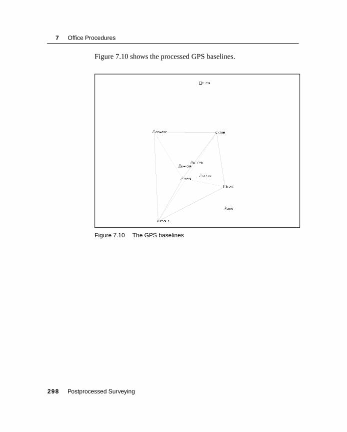
7 Office Procedures
Figure 7.10 shows the processed GPS baselines.
Figure 7.10 The GPS baselines
298 Postprocessed Surveying
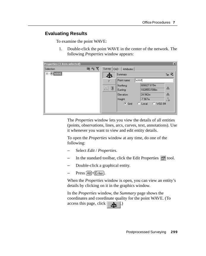
Office Procedures 7
7.14.2 Evaluating Results
To examine the point WAVE:
1. Double-click the point WAVE in the center of the network. The following Properties window appears:
The Properties window lets you view the details of all entities (points, observations, lines, arcs, curves, text, annotations). Use it whenever you want to view and edit entity details.
To open the Properties window at any time, do one of the following:
– Select Edit / Properties.
– In the standard toolbar, click the Edit Properties tool.
– Double-click a graphical entity.
– Press [Alt]+[Enter] .
When the Properties window is open, you can view an entity’s details by clicking on it in the graphics window.
In the Properties window, the Summary page shows the coordinates and coordinate quality for the point WAVE. (To access this page, click .)
Postprocessed Surveying 299
7 Office Procedures
2. Expand the tree on the left hand side of the Properties window to view the observations and keyed-in coordinates for the point WAVE.
3. The Point Derivation report shows how a recomputation determined the calculated position for the point WAVE. To view the report, select .
4. The Point Derivation report appears. In this case, the NEe coordinate in the control coordinates text file was adopted. The height was derived from the geoid model.
5. Close the report.
Viewing the GPS Baseline Processing report
To view the GPS Baseline Processing report for the baseline from MOON 2 to WAVE:
1. Select the baseline from MOON 2 to WAVE. In the Properties window, do the following:
a. Make sure that WAVE is still selected.
b. In the left pane, click the plus sign (+) next to the point name WAVE to show all of the observations for the point.
c. Select MOON 2-WAVE.
2. Select Reports / GPS Baseline Processing Report.
The GPS Baseline Processing report appears. Scroll through the report to view the baseline summary, the baseline components, and the tracking summary.
The report lets you assess whether the baseline processing has been successful, and check the entered field data. For example, you can check the satellite residuals.
3. Close the report.
300 Postprocessed Surveying
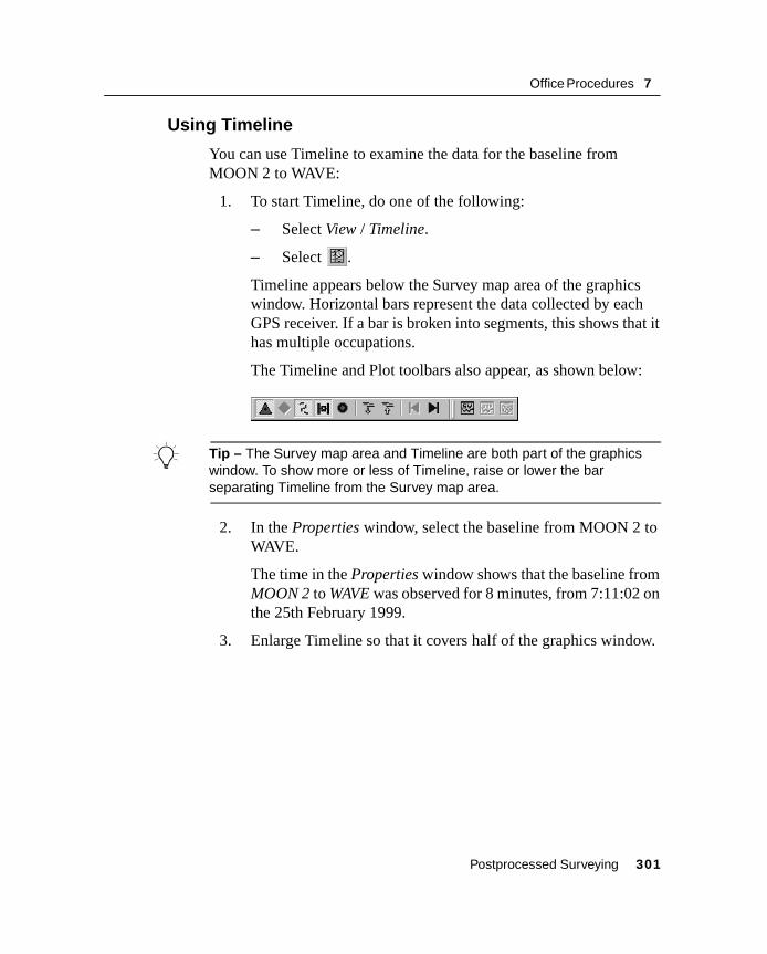
Office Procedures 7
7.14.3 Using Timeline
You can use Timeline to examine the data for the baseline from MOON 2 to WAVE:
1. To start Timeline, do one of the following:
– Select View / Timeline.
– Select .
Timeline appears below the Survey map area of the graphics window. Horizontal bars represent the data collected by each GPS receiver. If a bar is broken into segments, this shows that it has multiple occupations.
The Timeline and Plot toolbars also appear, as shown below:
B Tip – The Survey map area and Timeline are both part of the graphics window. To show more or less of Timeline, raise or lower the bar separating Timeline from the Survey map area.
2. In the Properties window, select the baseline from MOON 2 to WAVE.
The time in the Properties window shows that the baseline from MOON 2 to WAVE was observed for 8 minutes, from 7:11:02 on the 25th February 1999.
3. Enlarge Timeline so that it covers half of the graphics window.
Postprocessed Surveying 301

7 Office Procedures
Figure 7.11, shows the base receiver (MOON 2) and the roving receiver (WAVE) segments for the baseline. The bottom half of the observation segment bar is highlighted in a different color.
Figure 7.11 Timeline
4. In the file 4800:20116954, in the highlighted data segment, right-click to access the shortcut menu, and then select Zoom to Span. The data segment widens along the Timeline screen.
5. To expand the file, click the plus sign (+). This shows the satellites that were observed at WAVE.
6. To view the elevation data for satellite 26:
a. On SV 26, right-click to access the shortcut menu, and then select SV Plot. The Timeline-GPS Signal Plots window appears. You can use this window to view information about the satellites that were observed. For example, you can view the L1 and L2 signal-to-noise (SNR) ratios, the satellite azimuth, and the elevation.
b. Close the Timeline-GPS Signal Plots window.
7. To view information about each observation, double-click on an observation segment. The GPS Observation Properties dialog appears.
WAVEMOON 2
302 Postprocessed Surveying

Office Procedures 7
Note – If your GPS observations contain cycle slips, you can disable them. Drag a box around the cycle slip, then right-click to access a shortcut menu and select Disable, as shown below:
8. To close Timeline, select View / Timeline.
For more information about Timeline, refer to the Help.
Postprocessed Surveying 303
7 Office Procedures
7.15 GPS Loop ClosuresTo check the quality of, and identify any errors in, a set of GPS observations within a network, you can perform loop closures and then view the GPS Loop Closures report.
To set up the information to be displayed in the GPS Loop Closures report:
1. Select Reports / Setup / GPS Loop Closures Report. The Loop Closure Settings dialog appears.
2. In the Tolerance group, set the horizontal and vertical tolerance.
3. In the Report Sections group, select the sections to be displayed in the report.
To view the GPS Loop Closures report:
1. Select Reports / GPS Loop Closures Report. If you have observations selected, the Loop Closure Report dialog appears:
– In the Report on group, select the Whole database option and then click OK. The GPS Loop Closures report appears.
In the Summary section, the number of failed loops is 0. This shows that the GPS baseline loops close within the set tolerance, and that the data is ready for a network adjustment.
2. Close the report.
304 Postprocessed Surveying

Office Procedures 7
7.16A Guide to Least-SquaresAdjustment
In this section:
■ Least Squares
■ Error Types
■ Accuracy and Precision
■ Least-Squares Statistics
■ Normal Distribution
■ Standard Error
■ Variance and Weights
■ Standardized Residual
■ Review Questions
■ Answers
Postprocessed Surveying 305

7 Office Procedures
306 Postprocessed Surveying
Office Procedures 7
7.17 Least SquaresThe Trimble Geomatics Office software performs network adjustments using the least-squares technique. Before we address the issue of how is the adjustment done, we have to understand the basics of least squares and answer the question: What is to be adjusted?
The short answer is that an adjustment of errors is required.
It is impossible to measure any quantity and obtain an absolutely correct result. The measurement can only be made to a certain degree of accuracy, which is governed by:
• the instrument used
• the external conditions, and
• the observer
Regardless of the instrument quality and the observer’s skill, small discrepancies between repeated observations of the same quantity will always be present.
Some method must be devised for dealing with those discrepancies and combining the results to give the best mean result and an indicator of its reliability.
Least squares is the method that checks internal consistency of a network by showing how well individual observations fit with other observations in a data set. It highlights large errors, identifies bad observations in the network, handles random errors and computes reasonable error estimates for each observation.
Older methods, such as the compass rule, recognize the presence of larger errors, but can not identify bad observations. Consequently, errors are redistributed throughout the network, degrading adjustment results.
Postprocessed Surveying 307

7 Office Procedures
7.18 Error TypesVarious errors that occur in practice can be divided into three categories:
• Blunders
• Systematic Errors
• Random (accidental) errors
Least squares evaluates errors associated with a set of measurements.
7.18.1 Blunders
Blunders are a definite mis-reading of whatever scale is being used. Blunders are caused by the observer. These errors are usually large and are removed before performing a network adjustment.
Examples of blunders:
• Measuring the wrong antenna height
• Occupying the wrong survey point
• Entering the wrong station name
• Entering incorrect coordinates
7.18.2 Systematic Errors
Systematic errors are those errors that follow some fixed law (possibly unknown) dependent on the local environment. They are constant and are caused by the equipment. They are always of the same sign and tend to accumulate as more measurements are taken. Remove these errors before performing a network adjustment.
Systematic error examples:
• antenna height measurement tool that measures short or long
• antenna phase center variations
• tropospheric noise
308 Postprocessed Surveying

Office Procedures 7
7.18.3 Random Errors
Random errors are the remaining small errors after all the others just mentioned have been eliminated. Random errors are caused due to:
• instrument imperfections,
• the fallibility of the observer
• the changing conditions
They are revealed through repeated measurements, and impossible to remove completely.
Random error examples:
• atmospheric noise in the GPS signal
• interpolation error in measuring the antenna height
• tribrach centering error
Random errors follow the laws of probability. Removing large errors caused by mistakes and systematic errors allows least squares to detect random errors.
7.18.4 An Example of Errors
Using the same measurement tool, five people determined the distance measurement between the two points (to three decimal places) as shown below:
Observer Distance
1 5.675
2 5.667
3 5.671
4 5.676
5 5.680
Postprocessed Surveying 309

7 Office Procedures
Notice that the measurements are fairly consistent, with some small discrepancies.
If you take the mean of all the guesses you will see that all are within an acceptable error from the mean and that they are random.
But if someone in the group misinterpreted the integer 5 as a 6, then the error would be large and obvious. It would be outside the acceptable error. This can be considered a mistake, removed from the group, and a new mean calculated.
However, if all five people interpreted the integer to be 6 instead of 5, this would represent a systematic error. The correct value could be obtained by subtracting 1 from all the guesses or subtracting 1 from the mean. This would eliminate the systematic error.
310 Postprocessed Surveying

Office Procedures 7
7.19 Accuracy and PrecisionAccuracy is the closeness of a measurement to the actual value of the measured quantity. For example, when shooting bullets at a target, accuracy is the closeness of each bullet hole to the target’s center.
In contrast, precision is the repeatability of a particular measurement method. If each bullet hole is located the same distance and direction away from the center, the shooter is precise. It is possible to be accurate and not precise, and vice versa.
GPS is a very precise measurement method. GPS accuracy comes from your network design, control points used, satellite geometry, and redundant measurements. GPS accuracy comes from your application of the measurement method.
Accuracy and PrecisionHigh Accuracy and Low Precision
Accuracy and PrecisionLow Accuracy and High Precision
Postprocessed Surveying 311
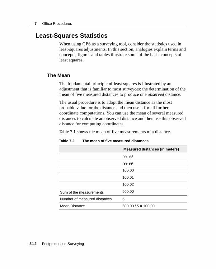
7 Office Procedures
7.20 Least-Squares StatisticsWhen using GPS as a surveying tool, consider the statistics used in least-squares adjustments. In this section, analogies explain terms and concepts; figures and tables illustrate some of the basic concepts of least squares.
7.20.1 The Mean
The fundamental principle of least squares is illustrated by an adjustment that is familiar to most surveyors: the determination of the mean of five measured distances to produce one observed distance.
The usual procedure is to adopt the mean distance as the most probable value for the distance and then use it for all further coordinate computations. You can use the mean of several measured distances to calculate an observed distance and then use this observed distance for computing coordinates.
Table 7.1 shows the mean of five measurements of a distance.
Table 7.2 The mean of five measured distances
Measured distances (in meters)
99.98
99.99
100.00
100.01
100.02
Sum of the measurements 500.00
Number of measured distances 5
Mean Distance 500.00 / 5 = 100.00
312 Postprocessed Surveying
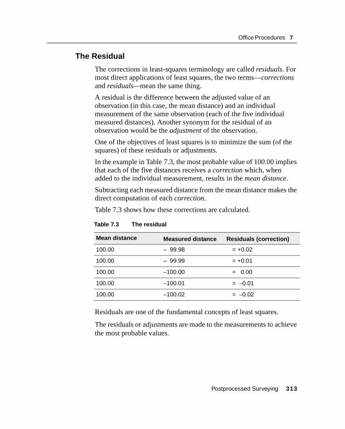
Office Procedures 7
7.20.2 The Residual
The corrections in least-squares terminology are called residuals. For most direct applications of least squares, the two terms—corrections and residuals—mean the same thing.
A residual is the difference between the adjusted value of an observation (in this case, the mean distance) and an individual measurement of the same observation (each of the five individual measured distances). Another synonym for the residual of an observation would be the adjustment of the observation.
One of the objectives of least squares is to minimize the sum (of the squares) of these residuals or adjustments.
In the example in Table 7.3, the most probable value of 100.00 implies that each of the five distances receives a correction which, when added to the individual measurement, results in the mean distance.
Subtracting each measured distance from the mean distance makes the direct computation of each correction.
Table 7.3 shows how these corrections are calculated.
Residuals are one of the fundamental concepts of least squares.
The residuals or adjustments are made to the measurements to achievethe most probable values.
Table 7.3 The residual
Mean distance Measured distance Residuals (correction)
100.00 – 99.98 = +0.02
100.00 – 99.99 = +0.01
100.00 –100.00 = 0.00
100.00 –100.01 = –0.01
100.00 –100.02 = –0.02
Postprocessed Surveying 313

7 Office Procedures
7.20.3 The Sum of the Squares of the Residuals Must be a Minimum
One of the criteria of a least-squares adjustment is that the sum of the squares of the residuals must be a minimum.
You have determined a mean for your measurements. Now, you must determine if the sum of the squares of the measurement residuals is a minimum.
Table 7.4 shows the sum of the squares of the residuals associated with the measurements from Table 7.3.
The sum of the squares of the residuals is determined to be 0.0010 by using the adjusted or most probable value of 100.00. Any value for the adjusted (most probable) distance other than 100.00 would result in different residuals, and the sum of the squares of the new residuals would be greater than 0.0010.
For example, if you arbitrarily used the adjusted distance of 99.99, you will find that after determining the new residuals, the sum of the squares of the residuals is 0.0015, showing that 0.0010 is the best answer. In this way, least squares satisfies the concept that the mean of the five measured distances is the best value for the unknown true distance.
Table 7.4 The sum of the squares of the residuals
Residuals Squares of the residuals (v2)
+ 0.02 0.0004
+ 0.01 0.0001
0.00 0.0000
- 0.01 0.0001
- 0.02 0.0004
Sum = 0.0010
314 Postprocessed Surveying
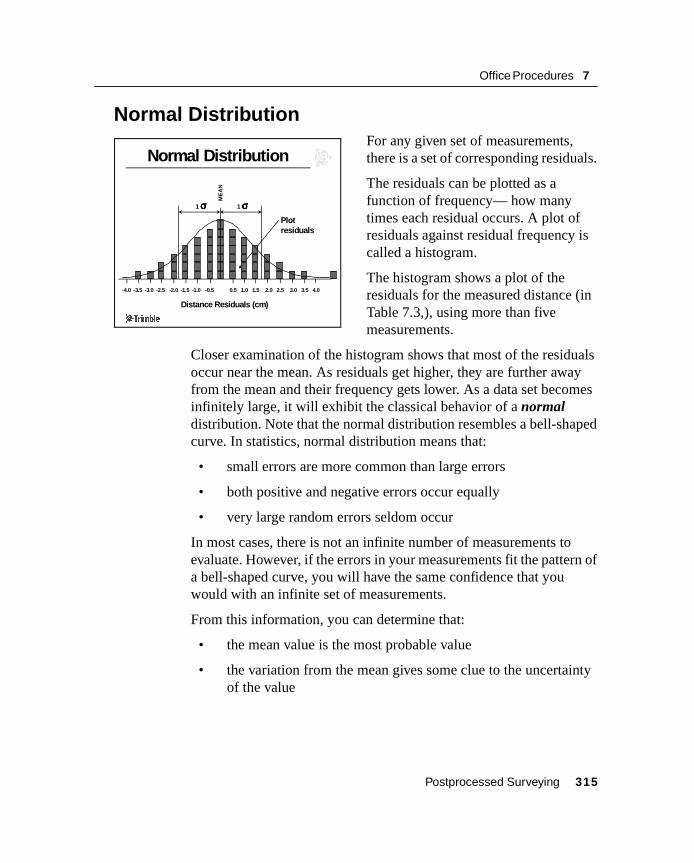
Office Procedures 7
7.21 Normal DistributionFor any given set of measurements, there is a set of corresponding residuals.
The residuals can be plotted as a function of frequency— how many times each residual occurs. A plot of residuals against residual frequency is called a histogram.
The histogram shows a plot of the residuals for the measured distance (in Table 7.3,), using more than five measurements.
Closer examination of the histogram shows that most of the residuals occur near the mean. As residuals get higher, they are further away from the mean and their frequency gets lower. As a data set becomes infinitely large, it will exhibit the classical behavior of a normal distribution. Note that the normal distribution resembles a bell-shaped curve. In statistics, normal distribution means that:
• small errors are more common than large errors
• both positive and negative errors occur equally
• very large random errors seldom occur
In most cases, there is not an infinite number of measurements to evaluate. However, if the errors in your measurements fit the pattern of a bell-shaped curve, you will have the same confidence that you would with an infinite set of measurements.
From this information, you can determine that:
• the mean value is the most probable value
• the variation from the mean gives some clue to the uncertainty of the value
Normal Distribution
4.0
Plotresiduals
ME
AN
0.5 1.0 1.5 2.0 2.5 3.0 3.5-0.5-1.0-1.5-2.0-2.5-3.0-3.5-4.0
Distance Residuals (cm)
1 σσσσ 1 σσσσ
Postprocessed Surveying 315
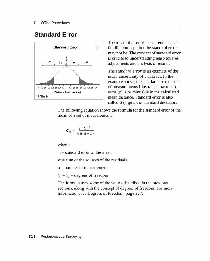
7 Office Procedures
7.22 Standard ErrorThe mean of a set of measurements is a familiar concept, but the standard error may not be. The concept of standard error is crucial to understanding least-squares adjustments and analysis of results.
The standard error is an estimate of the mean uncertainty of a data set. In the example above, the standard error of a set of measurements illustrates how much error (plus or minus) is in the calculated mean distance. Standard error is also called σ (sigma), or standard deviation.
The following equation shows the formula for the standard error of the mean of a set of measurements:
where:
m = standard error of the mean
v2 = sum of the squares of the residuals
n = number of measurements
(n – 1) = degrees of freedom
The formula uses some of the values described in the previous sections, along with the concept of degrees of freedom. For more information, see Degrees of Freedom, page 327.
Standard Error
4.0
ME
AN
0.5 1.0 1.5 2.0 2.5 3.0 3.5-0.5-1.0-1.5-2.0-2.5-3.0-3.5-4.0
Distance Residuals (cm)
1 σσσσ 1 σσσσ2 σσσσ 2 σσσσ
σmΣv2
n n 1–( )--------------------=
316 Postprocessed Surveying

Office Procedures 7
When you calculate a mean, there is an associated standard error. Continuing with the example, the mean distance is 100.00 ± 0.0071 m (where the standard error is 0.0071). An acceptable distance is anywhere between 99.9929 and 100.0071. The units of the standard error are the same as the units of the measured quantity. The common symbol for standard error is sigma (σ). The standard error is a useful statistical parameter because it defines the degree of confidence of the results.
• A 1-sigma error, which is the degree of confidence calculated above, corresponds to 68% confidence.
• This 1-sigma error equates to saying 68% of all measurements made under the same conditions will be within the stated standard error of the mean.
• Continuing with the example, repeated measurements of the distance might indicate that 68% of those distances would be somewhere between 99.9929 and 100.0071.
When surveying, you need a high level of confidence in your results. Errors for most surveys are often reported at 95% confidence or 1.96-sigma. The Trimble Geomatics Office software allows you to display the desired confidence level when choosing the adjustment style.
Note – Consult your project specifications for the required confidence levels for your reported results.
You determine 95% confidence in your results by applying a scalar to the standard error (sigma).
• We can calculate a 95% level of confidence by multiplying 0.0071 m by 1.960, which now sets our error statement at 0.0139.
• The Trimble Geomatics Office software handles all of the values and computations after you have configured your adjustment. At 95%, your mean distance is now 100.000.014 m.
• This means that if you measured the distance 100 times, 95 of those measurements will fall within 14 mm of the mean.
Postprocessed Surveying 317
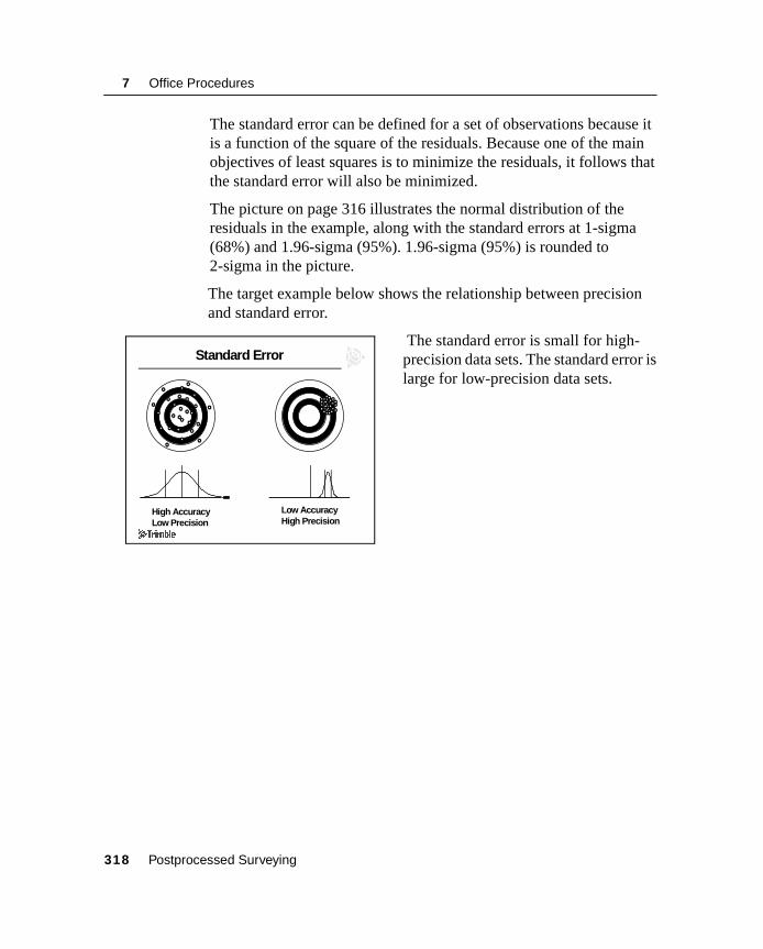
7 Office Procedures
The standard error can be defined for a set of observations because it is a function of the square of the residuals. Because one of the main objectives of least squares is to minimize the residuals, it follows that the standard error will also be minimized.
The picture on page 316 illustrates the normal distribution of the residuals in the example, along with the standard errors at 1-sigma (68%) and 1.96-sigma (95%). 1.96-sigma (95%) is rounded to 2-sigma in the picture.
The target example below shows the relationship between precision and standard error.
The standard error is small for high-precision data sets. The standard error is large for low-precision data sets.
Standard Error
High AccuracyLow Precision
Low AccuracyHigh Precision
318 Postprocessed Surveying
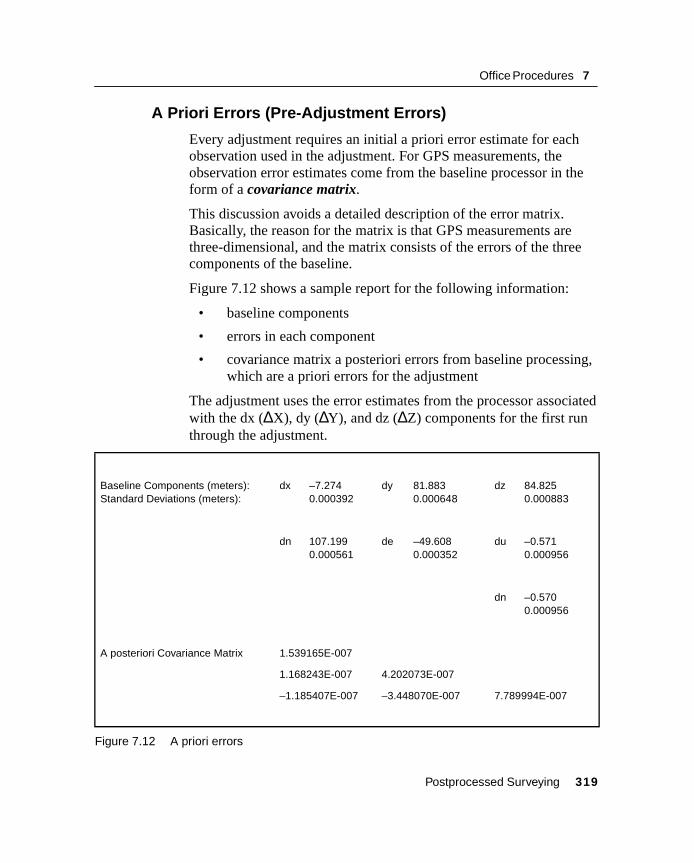
Office Procedures 7
7.22.1 A Priori Errors (Pre-Adjustment Errors)
Every adjustment requires an initial a priori error estimate for each observation used in the adjustment. For GPS measurements, the observation error estimates come from the baseline processor in the form of a covariance matrix.
This discussion avoids a detailed description of the error matrix. Basically, the reason for the matrix is that GPS measurements are three-dimensional, and the matrix consists of the errors of the three components of the baseline.
Figure 7.12 shows a sample report for the following information:
• baseline components
• errors in each component
• covariance matrix a posteriori errors from baseline processing, which are a priori errors for the adjustment
The adjustment uses the error estimates from the processor associated with the dx (∆X), dy (∆Y), and dz (∆Z) components for the first run through the adjustment.
Figure 7.12 A priori errors
Baseline Components (meters):Standard Deviations (meters):
dx –7.2740.000392
dy 81.8830.000648
dz 84.8250.000883
dn 107.1990.000561
de –49.6080.000352
du –0.5710.000956
dn –0.5700.000956
A posteriori Covariance Matrix 1.539165E-007
1.168243E-007 4.202073E-007
–1.185407E-007 –3.448070E-007 7.789994E-007
Postprocessed Surveying 319

7 Office Procedures
7.23 Variance and WeightsTrimble Geomatics Office weights an observation based on the variance of that observation. The variance is the square of the standard error, and weights are inversely proportional to the variance. Higher precision measurements have lower variances and greater weights. Trimble Geomatics Office applies more adjustment to observations with low weights.
This section introduces the concept of weighted measurements. There is no need to use weights in a network if all measurements are of:
• the same type (for example, all FastStatic observations)
• equal reliability
Typically, the above situation is rare. Use weights for your measurements when there are several types of measurements (for example, FastStatic, and kinematic), and when the measurements have different levels of precision and reliability.
Some reasons for different results for levels of precision and reliability may be:
• using differing methods of measurement
• observing for longer periods of time (or collecting differing numbers of observations)
• using instruments of differing orders of precision
• taking measurements over lines of differing lengths
• using different satellite constellations.
The more-reliable measurements in a network should receive smaller corrections in the adjustment than the less-reliable measurements. Weighting the measurements achieves this goal. The more-reliable measurements are assigned larger weights in the adjustment than the less-reliable measurements. The general theory is easy to apply.
Every measurement has a standard error.
320 Postprocessed Surveying
Office Procedures 7
To compute the weight for each measurement from the standard error:
• Determine the variance of the measurement. The variance is the standard error squared (σ2).
• Invert the variance to determine the weight associated with the measurement (1/σ2).
By inverting the variance, a smaller variance will become a larger number, thus a higher weight. A larger variance becomes a smaller number, thus a lower weight.
To fully understand weighted measurement, remember the following rules:
• Observations with small standard errors (small variance) get large weights, and observations with large standard errors (large variance) get small weights.
• Observations with large weights get small residuals (corrections), and observations with small weights get large residuals (corrections).
After weights are computed for each observation, the least-squares criteria are revised to the following:
• The network must close mathematically and geometrically.
• The sum of the weighted squares of the residuals must be a minimum.
With GPS surveying, allowing a least-squares adjustment to distribute the weights and errors is the most reliable method. Now, you are confident that the network is truly closed mathematically, and you have minimized the sum of the weighted squares of the residuals.
Postprocessed Surveying 321
7 Office Procedures
7.23.1 Variance Groups
With surveys, there are often varying groups of measurements used in a single network. The measurements can differ in several ways, including:
• the method of collection – GPS and terrestrial observations
• the type of measurements
The adjustment must have a way of accounting for the differing errors associated with these measurements. In the 5700 software, variance groups provide the ability to separate these measurements.
It is easy to see that the more precise the surveying methods, the smaller the measurement errors. The following example uses conventional surveying to explain why measurements are divided into variance groups.
Variance Groups for Conventional Surveying
As an example of variance groups for conventional surveying, consider the following. During a traverse to establish horizontal and vertical control on six points, the following methods were used to establish the vertical control on the points:
• Trigonometric elevations (from vertical angles) with a 10" theodolite were used to establish the difference in elevation between three of the points.
• A level with micrometer was used for determining the difference in elevation of the other three points.
The measurements using the level are more precise (smaller standard errors) than the trigonometric elevations. You do not want the same amount of adjustment (more correctly, weight) applied to the differential leveling as is applied to the trig elevations.
By dividing the two groups of measurements into variance groups and using variance group weighting strategy:
• the adjustment will apply different scalars to each group, based on the group’s estimated errors.
322 Postprocessed Surveying
Office Procedures 7
• separate reference factors and degrees of freedom are generated for each group, allowing analysis of each group’s quality of fit. This prevents the large errors (hence large adjustments) of the weaker measurements from being smeared (spread) across the entire network.
• the large errors stay with the weak measurements, and the small errors stay with the stronger measurements.
Variance Groups for GPS Surveying
For GPS surveying, divide the different types of GPS observations into separate groups based on different observation methods and solution type. Consider the following:
• The occupation times of the methods are key factors in the processor’s ability to properly model the error in the baseline.
• Occupation times decrease from static to FastStatic, and become very short with the kinematic methods.
• More error is usually associated with kinematic surveys due to use of a range pole when occupying the points.
You might prefer to separate longer baselines from the shorter baselines. The two types of baseline solutions can have varying errors due to:
• using the precise ephemeris for long baselines, and not using it with short baselines in baseline processing
• the effects of the atmosphere over long lines (iono free versus L1 fixed).
Another factor is the different types of baseline solutions. You may consider separating the baseline iono free solutions from the L1-fixed baseline solutions.
For more information on baseline processing, refer to the Trimble Geomatics Office Software – WAVE Baseline Processing User Guide.
Postprocessed Surveying 323
7 Office Procedures
7.24 Standardized ResidualGPS baselines consist of three components: azimuth, distance, and ellipsoid height. Residuals for these measurements are produced in both meters (linear) and degrees (angular), complicating the ability to compare residuals directly. The residuals of the azimuth cannot be directly compared to the residuals of the distance and delta height.
Because least squares deals with different types of observations, there is a need to directly compare residuals of different units.
The Trimble Geomatics Office software uses standardized (unitless) residuals rather than residuals of differing units, allowing you to directly compare quantities of different units.
Note – The observations in the adjustment are now represented as azimuth, distance, and delta height. In the section, A Priori Errors (Pre-Adjustment Errors), page 319, the observations (baselines) were represented as dx, dy, and dz. Once in the adjustment, the observations (along with associated errors) are transformed to a local geodetic horizon, displaying the observations in more familiar terms.
The process of producing standardized residuals from residuals of differing units is simple.
• A residual is calculated for every observation (or in the case of a GPS measurement, the components of the baseline).
• For each observation residual, a standard error is calculated as part of the adjustment.
• The standardized residual is computed by dividing the residual of an observation by the standard error (σ) of that residual.
324 Postprocessed Surveying

Office Procedures 7
Since the standardized residuals from each component have the same units, the resulting quotient is unitless, as shown in Table 7.5.
Compare each component (observation) of the baseline to each other. The residuals are difficult to compare directly, but in the standardized residual column you can make a straightforward comparison of the magnitude of the error in each observation component.
Table 7.5 Comparing standardized residuals
Observation Residual Standard error of the residual
Standardized residual1
1. Standardized residuals = residual/standard error of the residual
Azimuth +0.0806" 0.1032" 0.78
Distance –0.0353 m 0.0488 m 0.72
∆ Ellipsoid height –0.0284 m 0.0364 m 0.78
Postprocessed Surveying 325

7 Office Procedures
7.24.1 Histogram of Standardized Residuals and Tau Criterion
How do we use standardized residuals to evaluate baseline solutions and a least squares adjustment? A histogram of the standardized residuals shows how well Trimble Geomatics Office estimates the errors. Small errors occur more frequently than larger errors, and the probability and frequency of a positive or negative error is the same.
Two additional items are added to the histogram:
• The Critical tau values
• The Outliers
At this point in the adjustment:
• Blunders are eliminated from the adjustment.
• The systematic errors are modeled.
• The plot of the residuals shows only random errors.
There is always a possibility of a large random error—an error in an observation that is not consistent with the rest of the errors. Do not be alarmed by the presence of high standardized residuals. It now becomes a matter of what is acceptable and what is not. A limit on the magnitude of the standardized residual must be determined.
Trimble Geomatics Office performs a Tau criterion test to determine acceptable random error.
High standardized residuals identify large random error. The critical tau (τ) value is based upon the size, degrees of freedom, and desired confidence level for a given data set. If standardized residuals exceed the critical τ value, these residuals are outliers.
Tau Criterion
σσσσ 1 2 3 41234
Critical ττττ Critical ττττ
Outliers Outliers
326 Postprocessed Surveying
Office Procedures 7
Outliers are observations that do not fit well statistically with the rest of the data set. They are candidates for rejection because they adversely affect adjustment results.
If Trimble Geomatics Office flags an observation as an outlier, the software statistically rejects it. If this observation is not removed, you must justify keeping it!
7.24.2 Degrees of Freedom
In the Trimble Geomatics Office software, degrees of freedom is defined as the number of independent observations beyond the minimum required to uniquely define the unknown quantities.The strength of and confidence in the solution increases as the degrees of freedom increase. In a least-squares adjustment, try to maximize the degrees of freedom to help detect blunders and to correctly distribute the error in the measurements. This is also called adding redundancy to the network or observations.
One key aspect to degrees of freedom is the requirement to use independent observations:
In the formula for standard error (page 316), the degrees of freedom (n – 1) are in the denominator. So as you erroneously increase n – 1, you determine the square root of a smaller number and the standard error becomes smaller and smaller. If you falsely add distance observations of 100.00 to the example then recompute the standard error, you will see how it decreases—incorrectly indicating better results. For more information, see Standard Error, page 316.
In GPS surveying, a session is defined as static collection of simultaneous data with two or more receivers. When surveying with GPS, pay attention to independent and dependent observations. The number of independent observations in a GPS survey session equals n – 1, with n representing the number of receivers used in the session.
Postprocessed Surveying 327
7 Office Procedures
7.24.3 Reference Factor (Standard Error of Unit Weight)
The reference factor is another indicator for testing the quality of measurements and isolating suspect measurements. Reference factor is defined as a measure of the magnitude of observational residuals in an adjusted network as compared to estimated preadjustment observational errors. It is also called the standard error of unit weight.
A network adjustment makes small corrections (residuals) to the observations to make them fit well with each other. You must determine if these corrections are acceptable and reasonable.
If observational errors have been accurately estimated, you can expect that, on average, the residual received by each observation will be about the same size as its estimated error. In any adjustment, some observations will receive corrections smaller than their estimated errors, and some will receive larger. It can be demonstrated mathematically that if the estimated errors for an observation have been accurately estimated, the reference factor will be about 1.00.
A reference factor is computed for each observation and for the entire network. Use the network reference factor to determine if the errors are properly estimated for the entire network. For this discussion, it is simply stated as the overall amount of adjustment in the network, compared to the overall amount of estimated error in the network.
The reference factor is about 1.00 when the amount of the adjustment to the observations equals the estimated errors of those observations. With this information, you can determine the following:
• If the reference factor is less than 1.00, then the errors have been overestimated, and the network exceeds the precision estimated for it.
• If the reference factor is greater than 1.00, it indicates that, for a variety of reasons, one or more (or all) of the estimated errors have been underestimated.
In either case, more reasonable error estimates must be determined.
Note – An inflated reference factor can also indicate a blunder.
328 Postprocessed Surveying

Office Procedures 7
At this point, you must investigate why the reference factor does not equal 1.00. In the case where the reference factor is greater than 1.00, do the following:
• Remove all outliers or statistically justify them.
• Begin applying a scalar to your estimated errors to bring them in line with the residuals of the observations.
7.24.4 Chi-Square Test
Another test of the integrity of your adjusted network is an overall test of the adjustment statistics. This test is based upon the following:
• sum of the weighted squares of the residuals
• degrees of freedom
• critical probability of 95% (in the Trimble Geomatics Office software)
In some cases, the estimated errors are considered valid even though the reference factor exceeds 1.0. This is true when the network adjustment passes the Chi-square probability test.
The purpose of the test is to accept or reject the hypothesis that the predicted errors have been accurately estimated. The Trimble Geomatics Office software computes the probability percentage (level of significance) for the adjusted network. If this is greater than or equal to 95%, the reference factor passes the Chi-square test.
Failure of the Chi-square test indicates that you should do one of the following:
• Revise some or all of the predicted errors of the observations.
• Reject and possibly reobserve some or all of the observations.
• Use a combination of both of the above.
Postprocessed Surveying 329
7 Office Procedures
7.24.5 Scaling Your Estimated Errors
When performing an adjustment, it is possible that the reference factor exceeds 1.00 and the Chi-square test fails. These results indicate that the estimated observational errors are underestimated and do not match the amount of adjustment made to the observations.
When processing GPS baselines, there are limited data from which to calculate good error estimates. This could easily give rise to a reference factor (RF) > 1.
To better model the network errors, apply a scalar to the estimated errors. In the alternative scaling example below, if after the first adjustment the reference factor is 1.72 and the Chi-square test fails, this indicates that the errors are underestimated. Increase the estimated error by some scalar to properly model the network error. There are two considerations:
• Determine what value to use as the scalar.
• Determine the best estimate of the error in the network.
For both considerations, the answer is the reference factor (RF). In the Trimble Geomatics Office software, using the RF as the scalar for the next adjustment is called alternative scaling. This is an iterative process. Three strategies for applying a scalar to the estimated errors are as follows:
1. Apply a scalar to each observation. This equates to using the individual observation RF as the scalar that is applied to each estimated error in the next iteration of the adjustment.
2. Apply the network reference factor globally to each observation’s estimated errors: All Observations. This is the strategy used in the alternative scaling example below.
3. Apply a scalar to the Variance Groups. For more information, see Variance Groups, page 322.
330 Postprocessed Surveying

Office Procedures 7
Alternative scaling example
As an example, consider that the default scalar strategy is used during the first adjustment of a network. The default scalar value is always 1.0. The estimated errors are used at their face value to produce the reference factor of 1.72.
Note – To simplify this example, there are no outliers in the adjustment.
Using the alternative scalar strategy for the second adjustment automatically multiplies the first scalar value (1.0) by the current adjustment RF value (1.72), making the new scalar 1.72. During the second adjustment the new, scaled estimated errors are applied and the new RF is closer to 1.0.
If the reference factor is still greater than 1.0 (in this case, 1.50), then a new scalar is calculated by multiplying the latest reference factor (1.50) by the previous scalar (1.72) to produce a scalar (1.00 × 1.72 × 1.50 = 2.58) for the third adjustment. This process is continued until the reference factor approaches 1.0 and the Chi-square test passes.
B Tip – This process can be performed automatically using the Automatic Scalar Type option.
The observation error estimates may be approaching their true value when:
• The reference factor approaches 1.0.
• The histogram represents a bell-shaped curve.
Note – If the histogram appears as a narrow spike, then a lot of observations have had their error estimates over-inflated by the scaling. This is due to the presence of a bad observation. When the combined histogram appears to be normally distributed with no outliers, you can be confident that the overall weighting strategy is being applied correctly.
Postprocessed Surveying 331

7 Office Procedures
You now will have confidence in your results—both statistically and geometrically. When globally scaling, you improve the confidence of your error modeling and statistics without drastically changing your observations. This insures that the appropriate adjustments are made where needed in the network, and you are seeing a true representation of the errors in your final results.
Some analysis of the magnitude of the initial RF must be made when using a scalar. If the RF is a high, you will begin scaling the estimated errors by a large amount, then with subsequent iterations, the scalar will increase at a considerable rate. This is not a good practice. If the RF is high (inflated), it usually indicates a blunder still exists in the observations. The blunder must be removed from the adjustment before you can proceed with using a scalar.
B Tip – RTK and kinematic baselines produce a priori errors that are not as well defined as those for static baselines. You should be more concerned about static baselines with a large RF than about RTK and kinematic baselines with a large RF.
When performing an adjustment, consider the following guidelines:
• In a proper adjustment, you are evaluating and applying a scalar only to random errors. All other errors are removed or modeled.
• Observations with large random errors are flagged as outliers, and in most cases must be removed from the adjustment.
Note – Scale the estimated errors of the outliers using alternative scaling before excluding them from the adjustment. In some cases, scaling the estimated errors will allow the bad observation to fall within the critical tau value.
332 Postprocessed Surveying
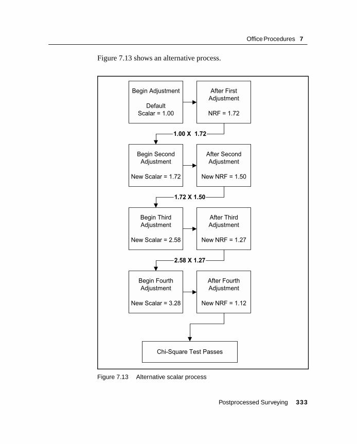
Office Procedures 7
Figure 7.13 shows an alternative process.
Figure 7.13 Alternative scalar process
After First
Adjustment
NRF = 1.72
Begin Second
Adjustment
New Scalar = 1.72
After Second
Adjustment
New NRF = 1.50
After Third
Adjustment
New NRF = 1.27
After Fourth
Adjustment
New NRF = 1.12
Begin Third
Adjustment
New Scalar = 2.58
1.00 X 1.72
1.72 X 1.50
2.58 X 1.27
Begin Adjustment
Default
Scalar = 1.00
Chi-Square Test Passes
Begin Fourth
Adjustment
New Scalar = 3.28
Postprocessed Surveying 333
7 Office Procedures
7.24.6 Observation Errors
Error estimates are necessary to perform a least squares adjustment. Conventional surveying error estimates come from equipment manufacturers’ specifications.
GPS equipment observation errors are loaded into the least-squares adjustment from the WAVE baseline processor results. An observation error is an error determined by the processing software. The Detailed Summary window in WAVE shows vector components (dx, dy, and dz) that correspond to baselines. Each component has a standard error.
The Detailed Summary also displays an a posteriori covariance matrix. Because GPS is a three-dimensional measurement, its error varies in three dimensions. Three-dimensional error estimates form a matrix. This matrix estimates observation errors when performing a network adjustment.
If RTK-observed data are used in a network adjustment, the Quality Control records (QC1 and QC2) must be attached to an observed position. This statistical covariance information is required for analysis of observational error.
334 Postprocessed Surveying
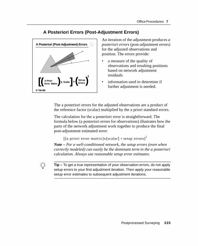
Office Procedures 7
7.24.7 A Posteriori Errors (Post-Adjustment Errors)
An iteration of the adjustment produces a posteriori errors (post-adjustment errors) for the adjusted observations and position. The errors provide:
• a measure of the quality of observations and resulting positions based on network adjustment residuals
• information used to determine if further adjustment is needed.
The a posteriori errors for the adjusted observations are a product of the reference factor (scalar) multiplied by the a priori standard errors.
The calculation for the a posteriori error is straightforward. The formula below (a posteriori errors for observations) illustrates how the parts of the network adjustment work together to produce the final post-adjustment estimated error:
Note – For a well-conditioned network, the setup errors (even when correctly modeled) can easily be the dominant term in the a posteriori calculation. Always use reasonable setup error estimates.
B Tip – To get a true representation of your observation errors, do not apply setup errors to your first adjustment iteration. Then apply your reasonable setup error estimates to subsequent adjustment iterations.
X +A PrioriError Matrix
2Set-upErrors( )[ ]
A Posteriori (Post-Adjustment) Errors
Scalar ( )
a priori error matrix )x scalar ] setup errors+( )2([
Postprocessed Surveying 335

7 Office Procedures
The network adjustment uses baseline solutions and observation errors to determine positions for unknown points. Sometimes observation error estimates are not realistic. Often, the network adjustment passes only if the error estimates are multiplied or scaled by some amount. Scaled error estimates are adjustment errors. These adjustment errors are a function of the observation errors and the setup errors. Adjustment errors are associated with final adjustment results and ultimately reported to clients.
336 Postprocessed Surveying

Office Procedures 7
7.24.8 Least-Squares Adjustment Review Questions
1. What are three types of errors in surveying?
2. List an example of each type of GPS error.
3. What error type is effectively evaluated by least squares?
4. What is the significance of the standard error?
5. How are weights related to the variance?
6. How does least squares identify a bad observation?
Postprocessed Surveying 337

7 Office Procedures
7.24.9 Least-Squares Adjustment Answers
1. Blunders, Systematic, Random
2. Examples:
– Blunders:
Wrong HI
Occupying wrong point
Entering wrong station name
– Systematic:
HI measuring tool too short
Antenna phase center variation
– Random:
Tribrach centering
Interpolation error in HI
Atmospheric noise in signal
3. Random error
4. The standard error defines the degree of confidence in measurement results.
5. Weights are inversely proportional to the variance.
6. Least squares flags observations with high standardized residuals that exceed the critical Tau value for a given data set.
338 Postprocessed Surveying

Office Procedures 7
7.25Network Adjustment
In this section:
■ Network adjustment procedures
■ Applying a scalar to the estimated errors
■ Adjusting terrestrial data
■ Performing a fully constrained adjustment
Postprocessed Surveying 339

7 Office Procedures
340 Postprocessed Surveying

Office Procedures 7
7.26 Network Adjustment ProceduresThe network adjustment occurs in two major steps.
The first step is the minimally constrained or free adjustment, which acts as a quality control check of your observations.
Use it to:
• check the internal consistency of the network
• detect blunders or ill-fitting observations
• obtain accurate observation error estimates
The second step is the fully constrained adjustment.
Use it to:
• reference the network to existing control (datum)
• verify existing control
• produce network transformation parameters (optional)
• obtain accurate coordinate error estimates
Both steps are required to obtain a complete adjustment and to provide confidence in your results. The adjustment definitions and procedures are discussed in the follow sections.
Postprocessed Surveying 341

7 Office Procedures
7.26.1 Minimally Constrained or Free Adjustment
A minimally constrained adjustment is an adjustment with only one control point held fixed in the survey network. Holding one control point fixed shifts observations to the correct location within the chosen datum. Not fixing a control point forces the software to perform a free adjustment. A free adjustment is accomplished by minimizing the size of the coordinate shift throughout the network. This equates to a mean coordinate shift of 0 (zero) in all dimensions.
A minimally constrained or free adjustment acts as one quality control check on the network. This adjustment helps to identify bad observations in the network. If an observation does not fit with the rest of the observations, it is highlighted as an outlier. The minimally constrained or free adjustment also checks how well the observations hold together as a cohesive unit.
Note – Perform a minimally constrained adjustment of GPS observations using WGS-84 as the adjustment datum. Since all GPS observations are made on the WGS-84 datum, the adjustment of the observations should be tied closely to the WGS-84 datum.
The minimally constrained adjustment is an iterative process:
• Perform an adjustment to check the observations for internal consistency and estimates errors for all observations. If bad observations are found, they appear as outliers in a histogram of standardized residuals.
• Remove these observations (one at a time, starting with the largest) so that the statistics of the network are not skewed.
• Perform the adjustment again; errors are estimated again.
In the subsequent adjustments, the estimated error may be rescaled to produce more realistic error estimates.
Repeat the process until the results meet the following conditions:
• All outliers have been removed from the network.
• Observations have the most accurate error estimates possible.
• Observations are adjusted such that they fit together well.
342 Postprocessed Surveying

Office Procedures 7
During the iteration process, two least-squares statistics are used to gauge progress:
• Reference factor – The reference factor shows how well the observations, along with their respective error estimates, are working together. Once the reference factor approaches 1.00, the errors in the observations are properly estimated and all observations have received their appropriate adjustments.
• Chi-square test – Typically when the reference factor approaches 1.00, the Chi-square test of network error estimates, degrees of freedom, and level of confidence will pass. As long as realistic setup errors were used in the adjustment, you can be confident that the network observations are working together and that there are no large errors remaining in the network.
Once the minimally constrained adjustment is complete, move on to the fully constrained adjustment to fit the observations to the local control datum.
Figure 7.14 and Figure 7.15 show the minimally constrained adjustment flow and the troubleshooting procedure, respectively.
Postprocessed Surveying 343
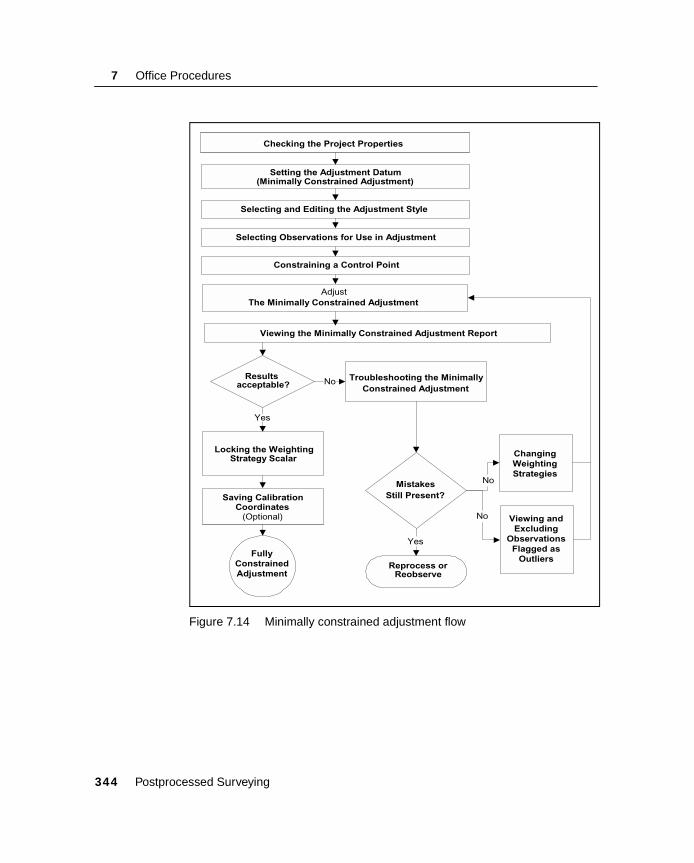
7 Office Procedures
Figure 7.14 Minimally constrained adjustment flow
Checking the Project Properties
Selecting and Editing the Adjustment Style
Setting the Adjustment Datum(Minimally Constrained Adjustment)
Constraining a Control Point
Viewing the Minimally Constrained Adjustment Report
Resultsacceptable?
Troubleshooting the MinimallyConstrained Adjustment
Viewing andExcluding
ObservationsFlagged as
Outliers
ChangingWeightingStrategies
Reprocess orReobserve
MistakesStill Present?
Yes
AdjustThe Minimally Constrained Adjustment
FullyConstrainedAdjustment
Selecting Observations for Use in Adjustment
Saving CalibrationCoordinates
(Optional)
Locking the WeightingStrategy Scalar
No
No
No
Yes
344 Postprocessed Surveying
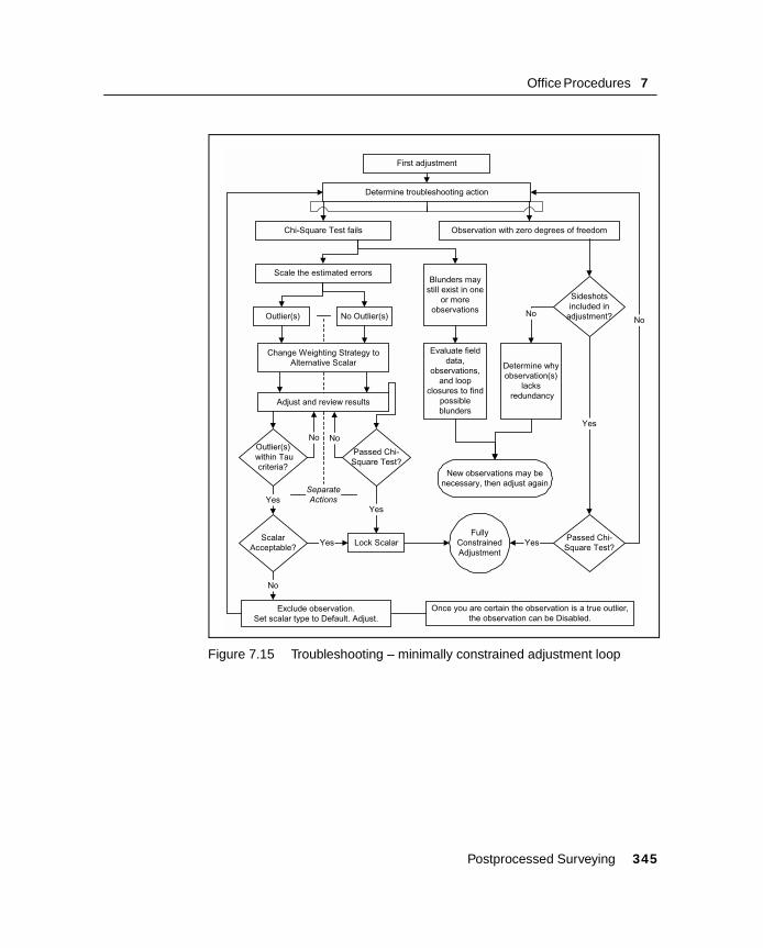
Office Procedures 7
Figure 7.15 Troubleshooting – minimally constrained adjustment loop
Exclude observation.Set scalar type to Default. Adjust.
Blunders maystill exist in one
or moreobservations
Observation with zero degrees of freedom
Outlier(s)
Determine troubleshooting action
No Outlier(s)
Determine whyobservation(s)
lacks redundancy
Passed Chi-Square Test?
FullyConstrainedAdjustment
First adjustment
Adjust and review results
Outlier(s) within Tau
criteria?
No
Yes
No
Chi-Square Test fails
No
Evaluate fielddata,
observations,and loop
closures to findpossibleblunders
Passed Chi-Square Test?
Yes
New observations may benecessary, then adjust again
ScalarAcceptable?
Yes
No
Yes
Separate
Actions
Sideshotsincluded in
adjustment?
Lock Scalar Yes
Change Weighting Strategy toAlternative Scalar
Scale the estimated errors
No
Once you are certain the observation is a true outlier,the observation can be Disabled.
Postprocessed Surveying 345

7 Office Procedures
7.26.2 Fully Constrained Adjustment
The fully constrained adjustment transforms the network of observations to the control points in the network. Once the network is fixed to those control points, adjusted coordinates (based on the project datum) for all other points in the network can be determined. Use this step to check that the existing control fits together well.
The minimally constrained adjustment showed that the observations fit together and a fairly rigid network is defined. It is assumed that if any large errors are present in the fully constrained adjustment, the source is nonhomogeneous control points (values). Any ill-fitting control points should not be fixed (constrained).
When designing the network, it is good practice to use a minimum of three horizontal control points and four vertical control points because:
• Two horizontal and three vertical control points are required to define transformation parameters.
• The additional horizontal and vertical control points can be used to check the consistency of the adjustment and defined transformation parameters.
Adding additional control points builds more confidence in the calculated parameters.
In the fully constrained adjustment, begin fixing the control values to determine how well the rigid network of observations fit the control. Essentially, the adjustment determines if the network of observations fit the network of fixed control points given some error estimate. These error estimates are the error estimates along with the applied scalar and setup errors. The transformation parameters are then calculated to allow the observations to fit to the control.
Note – If the measurements are made on the WGS-84 datum. You must provide control values (points) in your local datum that allow the adjustment to solve for the change in datum using calculated transformation parameters.
346 Postprocessed Surveying

Office Procedures 7
Figure 7.16 shows the fully constrained adjustment flow.
Figure 7.16 Fully constrained adjustment flow
Setting the Adjustment Datum(Fully Constrained Adjustment)
Constraining Control Points inthe Project Datum
The Fully ConstrainedAdjustment
Viewing a Fully ConstrainedAdjustment Report
AreAdjustment results
acceptable?
Generating a Final NetworkAdjustment Report
Troubleshooting the FullyConstrained Adjustment
Releasing a Control Point
Changing Weighting Strategiesfor Geoid Observations
Loading GeoidObservations
No
Locking the Weighting StrategyScalar for Geoid Observations
Yes
(if adjusting GPS data)
(if geoid observations have been loaded)
(if geoid observations have been loaded)
Postprocessed Surveying 347
7 Office Procedures
7.26.3 Transformation Analogy
This analogy will help you to understand the definition of the transformation parameters in a fully constrained adjustment. A simple transformation involves three parameters: rotation, scale, and deflection.
Defining the rotation
The rotation of the network (datum) can be defined by fixing two horizontal control points:
• Imagine the network as lines and named points on a piece of rubberized paper. The paper is rubberized to allow for any stretching or contracting (scaling) that might occur.
• Imagine a defined network of named control points marked on a wall.
• Use a tack to fix a point on the paper to the first control point with the same name on the wall.
• Let the paper hang freely. It will orient itself in an unpredictable direction.
• Now tack (fix) a second point on the paper to a point with the same name on the wall. The sheet of paper is rotated slightly to make the two points line up.
This is the measure of the rotation needed to fix the two networks together, allowing the observations to fit to the control values. The rotation is calculated but not checked.
• Tack a third point on the paper to the wall to check the rotation. You can determine how far the tack is from a point on the wall with the same name.
• If the tack is close to point on the wall (no large errors are seen), you are confident the rotation is defined correctly. This check is the same on all the parameters defined during the fully constrained adjustment.
348 Postprocessed Surveying

Office Procedures 7
Defining the scale
The scale of the network can be calculated by fixing one vertical point in addition to the two horizontal points. This concept gets a little more complicated. Continue with the above example:
• Imagine the piece of paper and the wall as curved surfaces, because you know the earth and the models used for coordinate computations are not flat.
• As you fix your first vertical control point, the paper is, perhaps, 10 cm from the wall. (The paper could also be 10 cm below the surface of the wall.) This is the difference between the two ellipsoids that define your datum.
• As you move the paper away from the wall, still holding the horizontal points, the horizontal distances between the points will become larger (and shorter if the paper is moved below the surface of the wall).
• The difference, or ratio, between two distances is defined as the scale factor. The definition is checked with additional horizontal and vertical control points.
Postprocessed Surveying 349

7 Office Procedures
Defining the deflection
As you fix additional vertical control points in the network, you define the network deflection (of the vertical). The deflection is the angular difference between the ellipsoid surface of one datum (WGS-84) and the ellipsoid surface of another datum (local). Continue with the above example:
• Now picture the wall as not only curved, but also an inclined surface. This inclination is the difference between the two ellipsoid surfaces.
• Model this inclination by fixing additional vertical control points. As you fix vertical points on the paper, the relationship to the incline of the wall is defined. The measurement of that inclination is the deflection (of the vertical) of your network.
By fixing two vertical points, the deflection in one direction is defined.
By fixing three points, the deflections in all three directions are defined. Adding more points allows you to check your definition of the vertical.
The transformation parameters are defined, allowing you to generate coordinates of the adjusted points in your local datum. The fully constrained adjustment is complete.
350 Postprocessed Surveying
Office Procedures 7
Exercise 21: Perform a Network Adjustment
Using Trimble 4700 and 4800 GPS Total Stations, survey crew A used Static/FastStatic methods to place control for a topo job.
Crew B combined the use of the Trimble 4800's and a Trimble GPS Total Station 5600 to collect topo data and traverse tie point DON to the control network.
Crew C used a Trimble DiNi to run differential levels from N 245 to KTOM to COWBOY to F 1239.
Crew B data are stored in file Topo.dc.
Crew C data are stored in file Level.dat.
Your task is to:
• Perform a minimally constrained adjustment of the GPS baselines and save the resultant coordinates for a GPS Site calibration.
• Import data obtained by Survey Crews B and C.
• Perform a minimally constrained adjustment of the terrestrial data.
• Perform a fully constrained adjustment of all data.
Setting up the project for minimally constrained adjustment for GPS data
The following sections show how to perform a minimally constrained adjustment of all data.
Display the ellipse controls
To display the Ellipse Controls toolbar, do one of the following:
• Select View / Toolbars / Ellipse Controls.
• Right-click on the Trimble Geomatics Office toolbar to access the shortcut menu, and then select Ellipse Controls.
Postprocessed Surveying 351

7 Office Procedures
In the toolbar, select the Error Ellipse tool to show the ellipses when the adjustment is performed.
Set the WGS-84 datum
To perform a minimally constrained adjustment of GPS data, select the WGS-84 datum.
To do this:
• Select Adjustment / Datum / WGS-84.
Set the adjustment style
You can set up the adjustment style to suit your project. In this example, use the 95% confidence limits for the adjustment style. To do this:
1. Select Adjustment / Adjustment Styles. The Network Adjustment Styles dialog appears.
2. In the Network Adjustment Styles dialog, select 95% Confidence Limits from the list and then click Edit.
3. In the 95% Confidence Limits dialog, select the Set-up Errors tab.
4. In the GPS group, do the following:
– In the Error in Height of Antenna field, enter 0.003.
– In the Centering Error field, enter 0.002.
5. In the Terrestrial group, do the following:
– In the Error in height of Instrument field, enter 0.003.
– In the Centering Error, enter 0.002.
6. To close each dialog, click OK.
352 Postprocessed Surveying

Office Procedures 7
Fixing the points in the network adjustment
To fix the points for the adjustment:
1. Do one of the following:
– In the Adjustment group of the project bar, click the Points shortcut.
– Select Adjustment / Points.
The following dialog appears:
2. In the Points dialog, select MOON 2.
3. In the Fix group, select the 2D check box.
4. Click OK.
The point MOON 2 is fixed in the adjustment.
Postprocessed Surveying 353

7 Office Procedures
Performing a Minimally Constrained Adjustment
To perform the adjustment, do one of the following:
– Select Adjustment / Adjust.
– In the Adjustment group of the project bar, click the Adjust shortcut.
Error ellipses will appear in the Survey view.
Viewing the Adjustment Results
To view the results of the adjustment, you need to view:
• the Network Adjustment report
• the Observations dialog
The following sections describe each task.
Viewing the Network Adjustment report
To view the Network Adjustment report:
1. Select Reports / Network Adjustment Report. The Network Adjustment report appears.
2. Maximize the report and in the Contents section, click Statistical Summary. (This summary is an important tool for analyzing the adjustment.)
The Chi-square test shows how well your observations fit together. However, in this adjustment, the Chi-square test fails. The network reference factor shows how well the observation errors are estimated. In this case, it exceeds 1.0.
3. Close the report.
When the Chi-square test fails and the network reference factor exceeds 1.0, this shows that the estimated observational errors are underestimated and do not match the amount of adjustment made to the observations.
354 Postprocessed Surveying
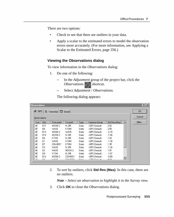
Office Procedures 7
There are two options:
• Check to see that there are outliers in your data.
• Apply a scalar to the estimated errors to model the observation errors more accurately. (For more information, see Applying a Scalar to the Estimated Errors, page 356.)
Viewing the Observations dialog
To view information in the Observations dialog:
1. Do one of the following:
– In the Adjustment group of the project bar, click the Observations shortcut.
– Select Adjustment / Observations.
The following dialog appears:
2. To sort by outliers, click Std Res (Max). In this case, there are no outliers.
Note – Select an observation to highlight it in the Survey view.
3. Click OK to close the Observations dialog.
Postprocessed Surveying 355
7 Office Procedures
7.27 Applying a Scalar to the Estimated ErrorsNote – When the Chi-square test fails and the network reference factor exceeds 1.0, this shows the estimated observational errors are underestimated and do not match the amount of adjustment made tothe observations. If there were no outliers we will need to apply a scalar.
To apply a scalar to the estimated errors:
1. Select Adjustment / Weighting Strategies. The Weighting Strategies dialog appears.
2. Make sure the GPS tab is selected.
3. In the Scalar Type group, select the Alternative option.
Using the alternative scalar strategy for the second adjustment automatically multiplies the first scalar value (1.0) by the current adjustment network reference factor value.
4. Click OK.
5. To readjust the network, select Adjustment / Adjust.
6. To view the Network Adjustment report, select Reports /Network Adjustment Report.
7. Maximize the report and in the Contents section, click Statistical Summary.
During the second adjustment, the new scaled estimated errors are applied. The Chi-square test still fails.
8. Close the report.
9. You can automate the process of applying a scalar to the estimated errors, using the automatic scalar option. To do this:
a. Select Adjustment / Weighting Strategies. The Weighting Strategies dialog appears.
b. Make sure the GPS tab is selected.
c. In the Scalar Type group, select the Automatic option.
d. Click OK.
356 Postprocessed Surveying

Office Procedures 7
The software performs an automatic adjustment, using the Alternative scalar type option. It repeats this adjustment until the global statistics are acceptable; that is, until the Chi-square test passes. For more information, refer to the Help.
10. Readjust the network and view the Network Adjustment report. The Chi-square test should now pass.
11. Close the Network Adjustment report.
Note – When you have finished performing a minimally constrained adjustment on the GPS data, you can save coordinates for a calibration by selecting Adjustment / Calibration Coordinates / Save.
Postprocessed Surveying 357
7 Office Procedures
7.28 Adjusting Terrestrial DataNow that all our GPS data has been adjusted on the WGS-84 datum we can proceed to import our terrestrial observations and adjust them on the Project datum.
7.28.1 Importing Terrestrial Data
The terrestrial data set that is used in the sample data is called Topo.dc.
To import it:
1. Select File / Import to open the Import dialog.
2. In the Survey tab, select the Survey Controller files (*.dc) option.
3. Click OK. The Open dialog appears. The Look in field defaults to the project’s Checkin folder.
4. Highlight the Topo.dc file.
5. Click Open.
The software imports the file and stores it in the Data Files\Trimble Files folder for the project.
Leveling observations or delta elevations often form part of the terrestrial adjustment network. You can also use them to improve the elevations derived from GPS observations. There is a Digital Level file included with the sample data.
To import data from a Digital Level file:
1. Select File / Import to open the Import dialog.
2. In the Survey tab, select the Digital Level files (*.dat, *.raw) option.
3. Click OK. The Open dialog appears. The Look in field defaults to the project’s Checkin folder.
4. Highlight the Level.dat file.
358 Postprocessed Surveying
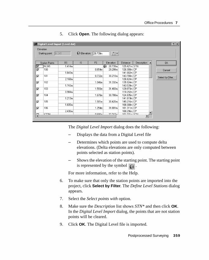
Office Procedures 7
5. Click Open. The following dialog appears:
The Digital Level Import dialog does the following:
– Displays the data from a Digital Level file
– Determines which points are used to compute delta elevations. (Delta elevations are only computed between points selected as station points).
– Shows the elevation of the starting point. The starting point is represented by the symbol .
For more information, refer to the Help.
6. To make sure that only the station points are imported into the project, click Select by Filter. The Define Level Stations dialog appears.
7. Select the Select points with option.
8. Make sure the Description list shows STN* and then click OK. In the Digital Level Import dialog, the points that are not station points will be cleared.
9. Click OK. The Digital Level file is imported.
Postprocessed Surveying 359
7 Office Procedures
Note – Editing the data in the Digital Level Import dialog does not edit the digital level file.
To view the digital level observations in the Properties window:
1. Select Select / Observations. The Observations dialog appears.
2. From the Type list, select the Delta Elevations check box and then click OK.
3. To open the Properties window, do one of the following:
– Select Edit / Properties.
– In the standard toolbar, click the Edit Properties tool.
– Press [Alt]+[Enter] .
When the Properties window is open, click on a specific level observation to view its details.
4. Close the Properties window.
7.28.2 Investigating Error Flags
When you import Topo.dc, error flags appear in the data. To investigate them, do one of the following:
• Double-click on the error flags in the graphics window.
• Double-click on the error flag shown in the status bar.
If you use the Flag icon in the status bar, all points with error flags appear in the Properties window.
To investigate these flags, you can view the point information in the Point Derivation report.
On point 1000, the flag is caused by the elevation and height on two check observations being out of tolerance. These two check observations do not match the enabled observation. This indicates that there may be something wrong with the observation.
360 Postprocessed Surveying
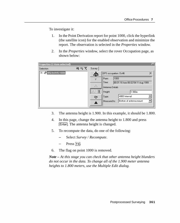
Office Procedures 7
To investigate it:
1. In the Point Derivation report for point 1000, click the hyperlink (the satellite icon) for the enabled observation and minimize the report. The observation is selected in the Properties window.
2. In the Properties window, select the rover Occupation page, as shown below:
3. The antenna height is 1.900. In this example, it should be 1.800.
4. In this page, change the antenna height to 1.800 and press [Enter]. The antenna height is changed.
5. To recompute the data, do one of the following:
– Select Survey / Recompute.
– Press [F4].
6. The flag on point 1000 is removed.
Note – At this stage you can check that other antenna height blunders do not occur in the data. To change all of the 1.900 meter antenna heights to 1.800 meters, use the Multiple Edit dialog.
Postprocessed Surveying 361
7 Office Procedures
7.28.3 Adjusting Terrestrial Observations
Note – In this sample data, there is not enough redundancy in the level data to perform the minimally constrained terrestrial adjustment without the GPS data present. In some cases, you may have enough redundancy to remove your GPS data before performing a minimally constrained terrestrial adjustment.
Setting the adjustment datum
To perform a minimally constrained adjustment on terrestrial observations, you will need to change the datum to the project datum. To do this:
• Select Adjustment / Datum / Project Datum – NAD 1983 Conus.
Creating a variance group for level observations
To create a separate variance group for the level observations in the adjustment, do the following:
1. Select Adjustment / Observation Groups / Variance Groups. The Variance Group dialog appears.
2. In the Terrestrial tab, click New. The New Variance Group dialog appears.
3. In the Name Group, enter Level Observations and then click OK. The Edit Variance Group dialog appears.
4. Click Filter. The Observation Filter dialog appears.
5. Clear all of the check boxes except Delta elev and click OK to return to the Edit Variance Group dialog.
6. In the Available Observations group, select the delta elevations observations and click Add. The delta elevation observations now appear in the Group observations field.
7. Click OK to return to the Edit Variance Group dialog.
8. Click Close.
362 Postprocessed Surveying

Office Procedures 7
Removing sideshots from the adjustment
The following example shows how to remove side shots from the adjustment:
1. To select the sideshot observations:
a. Select Select / Observations. The Select Observations dialog appears.
b. Make sure that the General tab is selected.
c. In the Type list, select the Terrestrial – Single face only check box.
d. Select the Side shots only check box.
e. Click OK.
The terrestrial sideshot observations are selected.
2. To remove the sideshot observations from the adjustment:
a. Select Edit / Multiple Edit. The Multiple Edit dialog appears.
b. In the Perform these edits to the selected observations group, select the Use in Network Adjustment option.
c. From the Use in Network Adjustment list, select No.
d. Click OK.
The sideshot observations will not be used in the network adjustment.
B Tip – You can also remove the sideshot observations from the adjustment using the Terrestrial tab in the Observations dialog. To do this, clear the Use check box for a highlighted observation. The Use check box for all of the other selected observations will also be cleared.
At this point in the adjustment, you will also need to load geoid observations so that the relationship between elevations (from terrestrial observations) and ellipsoid heights (from GPS observations) can be established.
Postprocessed Surveying 363
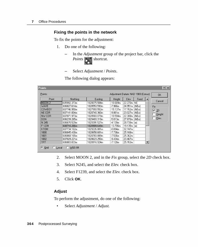
7 Office Procedures
Fixing the points in the network
To fix the points for the adjustment:
1. Do one of the following:
– In the Adjustment group of the project bar, click the Points shortcut.
– Select Adjustment / Points.
The following dialog appears:
2. Select MOON 2, and in the Fix group, select the 2D check box.
3. Select N245, and select the Elev. check box.
4. Select F1239, and select the Elev. check box.
5. Click OK.
Adjust
To perform the adjustment, do one of the following:
• Select Adjustment / Adjust.
364 Postprocessed Surveying
Office Procedures 7
• In the Adjustment group of the project bar, click the Adjust shortcut.
Viewing the Network Adjustment report
To view the Network Adjustment report:
1. Select Reports / Network Adjustment Report. The Network Adjustment report appears.
2. Maximize the report and in the Contents section, click Statistical Summary. (This summary is an important tool for analyzing the adjustment.)
The Chi-square test shows how well your observations fit together. The network reference factor shows how well the observation errors are estimated. In this case, the Chi-square test passes.
Note – You should also view the terrestrial observation statistics.
3. Close the report.
Scaling the errors
To scale the standard errors:
1. Select Adjustment / Weighting Strategies. The Weighting Strategies dialog appears.
2. Make sure that the Terrestrial tab is selected.
3. In the Apply Scalars To group, select the Variance Groups option.
4. In the Scalar Type group, select the Automatic option.
5. Click OK.
6. Select Adjustment / Adjust to readjust the network and then view the Network Adjustment report.
Postprocessed Surveying 365
7 Office Procedures
7. To scale the geoid observations:
a. Before scaling the geoid observations, you need to fix elevations. In the Points dialog, fix the elevations of the points N 245, WAVE, DON, and F 1239.
b. In the Weighting Strategies dialog – Geoid tab, select the Alternative scalar type option.
8. Select Adjustment / Adjust to readjust the network and then view the Network Adjustment report.
9. Click OK.
Loading geoid observations
When adjusting GPS observations, geoid observations are required to determine elevations on all the points in the adjustment.
You have worked with ellipsoid heights during the minimally constrained adjustment of your GPS observations. During the fully constrained adjustment you will begin fixing elevations to determine elevations for all the points with unknown elevations in the network.
Note – You do not need to load geoid observations when performing a horizontal adjustment.
To load geoid observations:
1. Select Adjustment / Observations. The Observations dialog appears.
2. In the Geoid tab, click Load. The geoid observations are loaded into the Observations group.
3. Click OK. You are now ready to fix a point in the network.
366 Postprocessed Surveying
Office Procedures 7
Applying a Scalar to the Geoid
The initial geoid separation error estimate is the standard error of the set of separations. The Trimble Geomatics Office software computes the geoid separations in the adjustment and then determines the standard error of those separations. This is only a starting point for the estimation of the errors in the geoid separation and may require that you scale the errors before a true representation of the estimated errors is achieved.
To apply a scalar to the Geoid:
1. Select Adjustment / Weighting Strategies. The Weighting Strategies dialog appears.
2. Make sure that the Geoid tab is selected.
3. In the Scalar Type group, select the Alternative option.
4. Using the alternative scalar strategy for the second adjustment automatically multiplies the first scalar value (1.0) by the current adjustment network reference factor value.
5. Click OK.
6. To readjust the network, select Adjustment / Adjust.
7. To view the Network Adjustment report, select Reports /Network Adjustment Report.
8. Maximize the report and in the Contents section, click Geoid Model.
9. Close the report.
You can automate the process of applying a scalar to the estimated errors, using the automatic scalar option. To do this:
1. Select Adjustment / Weighting Strategies. The Weighting Strategies dialog appears.
2. Make sure that the Geoid Model tab is selected.
3. In the Scalar Type group, select the Automatic option.
Postprocessed Surveying 367

7 Office Procedures
4. Click OK.
The software performs an automatic adjustment, using the Alternative scalar type option. It repeats this adjustment until the global statistics are acceptable; that is, until the Chi-square test passes. For more information, refer to the Help.
7.29 Performing a Fully Constrained AdjustmentThe minimally constrained adjustment has been successfully completed so you can now perform a fully constrained adjustment.
To do this:
1. Make sure that the adjustment datum is still set on the project datum.
2. You now need to generate the necessary transformations by constraining (fixing) the control points you have chosen to use in your network. The control points are usually well-established survey marks with high-accuracy horizontal (2D) or vertical coordinates.
3. To do this:
a. In the Points dialog, fix the following points:
– MOON 2 – NE
– N 245 – e
– WAVE – NEe
– DON – NEe
– F 1239 – e
b. Click OK.
Note – Perform an adjustment after fixing each point. This lets you check that each point is not contributing to errors in the adjustment.
368 Postprocessed Surveying

Office Procedures 7
4. Select Adjustment / Adjust to perform a fully constrained adjustment.
5. Select Reports / Network Adjustment Report to view the Network Adjustment Report. The Network Adjustment report appears.
6. View the information in the Statistical Summary section. The Chi-square test passes, indicating a successful adjustment. You can now view the adjusted coordinates for the file.
7. Close the Network Adjustment report.
8. In the toolbar, select the Error Ellipse tool to turn off the ellipse display.
For more information about network adjustments, refer to the Network Adjustment Help.
Postprocessed Surveying 369

7 Office Procedures
370 Postprocessed Surveying

C H A P T E R
8
Start to Finish 8In this chapter:
■ Introduction
■ Task review
■ Notes
8 Start to Finish
8.1 IntroductionYour skills should be complete on how to perform postprocessed surveying.
This chapter provides a test of the postprocessed surveying techniques offered in this course, using your Trimble equipment. Your instructor will provide you with a set of instructions to test your talent and confidence with your new skills.
8.2 Task ReviewIn order to demonstrate your level of understanding, you will:
• Create a project in Trimble Geomatics Office
• Plan the session and design a network
• Set up and configuring field equipment
• Start the survey
• Observe baselines as per session plan/network design
• Conduct TOPO survey using PPK technique
• End the survey
• Import and exporting data
• Process baselines
• Minimally and fully adjusting the network
372 Postprocessed Surveying

Start to Finish 8
8.3 Notes
Postprocessed Surveying 373

8 Start to Finish
374 Postprocessed Surveying

A P P E N D I X
A
Configuration AIn this appendix:
■ Introduction
■ Configuring the receiver in real-time
■ Configuring the receiver using application files
■ GPS Configurator
■ Configuration Toolbox
■ Default settings
A Configuration
A.1 IntroductionThe 5700 GPS receiver has no controls for changing settings. It can only be configured using external software such as GPS Configurator, Configuration Toolbox™, or Trimble Survey Controller.
Note – Options available in the software depend on the GPS receiver type connected.
Configure the GPS receiver by one of these methods:
• Configure the receiver in real time
• Apply the settings in an application file
This appendix provides a brief overview of each of these methods, and detailed information about the contents and use of application files.
A.2 Configuring the Receiver in Real-TimeGPS Configurator, Configuration Toolbox, and Trimble Survey Controller all support real-time configuration of the 5700 receiver.
When you configure the receiver in real time, use one of these software applications to specify which settings you want to change.
When you apply the changes, the receiver settings change immediately.
Any changes that you apply to the receiver are reflected in the Current application file, which is always present in the receiver. This file always records the most recent configuration, so if you apply further changes (either in real time or using an application file) the Current file is updated and there is no record of the original configuration.
376 Postprocessed Surveying

Configuration A
A.3 Configuring the Receiver Using Application FilesAn application file contains information for configuring a receiver. To use this method, you create the application file, transfer it to the receiver, and then apply the file’s settings. The Configuration Toolbox performs all of these tasks.
A.3.1 Application Files
An application file is organized into records, which store configuration information for a particular area of receiver operation.
Application files can include some or all of the following records:
• File Storage
• General Controls
• Serial Port Baud/Format
• Reference Position
• Logging Rate
• SV Enable/Disable
• Output Message
• Antenna
• Device Control
• Static/Kinematic
• Input Message
• Timed Activation
When you activate an application file, any option that is not included in the records in the file remains at its current setting. For example, if you use an application file that only specifies the elevation mask, all other settings remain as they were.
Postprocessed Surveying 377
A Configuration
You can store up to 20 different application files in battery-backed memory on the receiver, and apply its settings at the time it is transferred to the receiver, or at any time afterwards.
Special Application Files
The GPS receiver has three special application files, which control important aspects of the receiver’s configuration.
Default application file – This file (Default.cfg) contains the original receiver configuration, and cannot be changed. It configures the receiver after it is reset.
Although you cannot change or delete the default application file, you can use a Power Up application file to override any or all of the default settings.
Current application file – This file (Current.cfg) reflects the current receiver configuration. Whenever you change the receiver’s configuration, either in real time or by applying an application file, the Current file changes to match the new configuration.
You cannot delete the Current file or change it directly, but every change to the receiver’s current configuration is applied to the Current file as well.
When you switch off the receiver then turn it on again, all the settings from the Current application file are applied, so you do not lose any changes that you have made.
The only exceptions are the following logging parameters:
• Logging rate
• Position rate
• Elevation mask
These parameters are always reset to the factory default values whenever the receiver is switched off.
378 Postprocessed Surveying

Configuration A
Power Up application file – This file (Power_up.cfg) is optional. If a Power Up file is present, its settings are applied whenever the receiver is powered up.
Use the file to specify that the receiver is reset to defaults before the Power Up settings are applied. This ensures that restarting the receiver always results in the same configuration. This method is useful for defining “default” settings for the receiver that differ from those in the Default file, which cannot be changed.
Alternatively, you can specify that the Power Up settings are applied immediately after the Current application file’s settings have been applied. Restarting the receiver results in a configuration that uses your default settings for the options you define in the Power Up file, but the current settings for all other options.
By default, there is no Power Up application file on the receiver, so if you want to use one, you need to create an application file in Configuration Toolbox and make sure that the As auto power up file option is selected in the File dialog. When you transfer this file to the receiver, it is transferred with the name Power_up.cfg, and becomes the new Power Up file.
The Power Up file is the only special application file that you can overwrite or delete from the receiver.
Postprocessed Surveying 379
A Configuration
A.3.2 Timed Application Files
The 5700 receiver supports Timed Application files. These files contain Timed Activation records, which specify when the file is to be applied. The main use of a timed application file is to automatically start or stop logging at a predefined time.
The Timed Activation record specifies:
• the UTC date and time when the application file is to be applied for the first time.
• the interval at which the file is to be reapplied.
If you do not specify a repeat interval, the settings are applied only once, at the specified time. If the file specifies a repeat interval, the file’s settings are reapplied at the specified interval until the file is deactivated.
Defining timed application files
To send timed application files to a GPS receiver, set up scheduled survey sessions in GPS Configurator. You can define multiple sessions, each specifying:
• basic logging parameters (data logging rate, position logging rate, and elevation mask)
• a starting time
• a duration
When you apply the current settings in the GPS Configurator software, each defined survey session is sent to the GPS receiver as a pair of timed application files: the first includes the logging settings and start time, and the second contains settings that stop logging at the end time (which is calculated automatically from the duration you specify).
Note – You cannot use Configuration Toolbox to define timed application files.
380 Postprocessed Surveying
Configuration A
A.3.3 Sleep mode
Whenever you press Power to turn off the 5700 GPS receiver, it checks for a timed application file that is due to be activated in the future. If one exists, the receiver goes into Sleep mode instead of powering down. In Sleep mode, the yellow Logging/Memory LED flashes every three seconds. The receiver wakes up five minutes before the scheduled activation time, so that it is ready to begin logging at the scheduled time.
A.3.4 Activating Application Files
An application file’s settings do not affect the receiver’s configuration until you activate the application file. You can do this at the same time that you save the file. Alternatively, you can save the file on the computer or in the receiver, then open it later and apply its settings.
Note – If the application file is a timed file, its settings do not take effect as soon as you activate the file, but at the time that the file specifies for its activation.
A.3.5 Storing Application Files
You can store application files that you create in Configuration Toolbox on both your receiver and computer. For example, each file can represent a different user sharing the same receiver, or a particular mode of operation or survey style. Saving application files on your computer as well as in your receiver is optional, but it is useful because:
• it gives you a permanent copy of the settings you have sent to a receiver, for audit or your own reference.
• you can use the same file to configure multiple receivers identically.
• you can use an existing application file as a template for creating other application files with similar settings.
Postprocessed Surveying 381
A Configuration
A.3.6 Naming Application Files
The filename that you use to store the application file in the computer and the name under which the file is stored in the receiver are always the same. This makes it easier to recognize and keep track of your application files. If you change the filename on the receiver, the name of the application file on your computer also changes. Similarly, if you change the filename on your computer, the name of the file in the receiver changes.
382 Postprocessed Surveying
Configuration A
A.4 GPS ConfiguratorUse GPS Configurator to configure selected Trimble GPS receivers. With GPS Configurator you can:
• check current receiver settings and operation
• change receiver settings in real time
A.4.1 Configuring the GPS Receiver
To configure a GPS receiver using GPS Configurator:
1. Connect Port 1, 2, or 3 on the receiver to a serial (COM) port on the computer and switch on the power.
2. Click , then select Programs / Trimble / GPS Configurator / GPS Configurator.
The software automatically establishes a connection with the 5700 GPS receivers.
Postprocessed Surveying 383

A Configuration
The following dialog appears:
3. Select your receiver settings as required.
For more information, refer to the GPS Configurator Help.
4. Click Apply.
The settings in GPS Configurator are immediately applied to the receiver.
384 Postprocessed Surveying

Configuration A
A.5 Configuration ToolboxThe Configuration Toolbox software is a Windows application that provides a graphical user interface to help you configure selected Trimble GPS receivers.
With Configuration Toolbox you can:
• create and edit application files
• transfer application files to and from the receiver
• manage application files stored in the receiver
A.5.1 Creating an Application File
To create and save an application file to the receiver:
1. To start Configuration Toolbox, click , then select Programs / Trimble / Configuration Toolbox / Configuration Toolbox.
2. Select File / New / 5700. The following dialog appears:
3. Specify the receiver settings. For more information, refer to the Configuration Toolbox Help.
Postprocessed Surveying 385

A Configuration
4. Select File / Save As to save the application file:
To transfer the application file to the receiver:
1. Connect the data/power cable to Port 1 on the 5700 receiver.
2. Connect the female DB9 connector on the other end of the data/power cable to a serial (COM) port on the computer.
3. Select File / Open to open the required application file:
386 Postprocessed Surveying
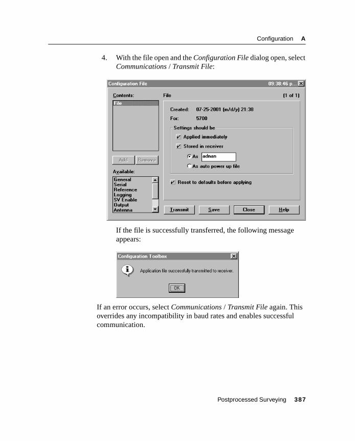
Configuration A
4. With the file open and the Configuration File dialog open, select Communications / Transmit File:
If the file is successfully transferred, the following message appears:
If an error occurs, select Communications / Transmit File again. This overrides any incompatibility in baud rates and enables successful communication.
Postprocessed Surveying 387

A Configuration
5. To check whether the transfer was successful, close the Configuration File dialog and select Communications / Get File:
A list of all application files in the 5700 receiver appears:
If you selected the Applied Immediately check box in the application file, the Current application file will contain the settings in the new file.
6. To apply a different file, select the file you require from the list and then select Communications / Activate File.
388 Postprocessed Surveying

Configuration A
A.6 Default SettingsTable A.1 defines the default settings for the 5700 receiver.
Table A.1 5700 receiver default settings
Function Factory default
SV Enable All SVs enabled
General controls:Elevation maskPDOP maskRTK positioning modeMotion
130
7Low LatencyKinematic
Power Output 3 Disabled
1PPS time tags Off
ASCII time tags Off
Serial Port 1:Baud rateFormatFlow control
384008-None-1None
Serial Port 2:Baud rateFormat
384008-None-1
Serial Port 3:Baud rateFormatFlow control
384008-None-1None
Input Setup:Station Any
NMEA/ASCII (all messages) All Ports Off
Streamed output All Types Off
Offset = 00
RT17/Binary All Ports Off
CMR output [Static] CMR:cref ID 0000
RTCM output RTCM: Type 1 ID 0000
Postprocessed Surveying 389
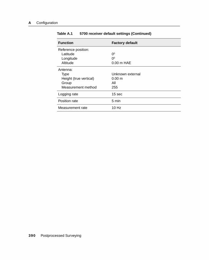
A Configuration
Reference position:LatitudeLongitudeAltitude
00
00
0.00 m HAE
Antenna:TypeHeight (true vertical)GroupMeasurement method
Unknown external0.00 mAll255
Logging rate 15 sec
Position rate 5 min
Measurement rate 10 Hz
Table A.1 5700 receiver default settings (Continued)
Function Factory default
390 Postprocessed Surveying

GlossaryThis section explains some of the terms used in this manual.
almanac Data, transmitted by a GPS satellite, that includes orbit information on all the satellites, clock correction, and atmospheric delay parameters. The almanac facilitates rapid SV acquisition. The orbit information is a subset of the ephemeris data with reduced precision.
Anti-Spoofing (AS)
A feature that allows the U.S. Department of Defense to transmit an encrypted Y-code in place of P-code. Y-code is intended to be useful only to authorized (primarily military) users. Anti-Spoofing is used with Selective Availability to deny the full precision of GPS to civilian users.
autonomous positioning
The least precise form of positioning that a GPS receiver can produce. The position fix is calculated by one receiver from satellite data alone.
base station In a GPS survey, you observe and compute baselines (the position of one receiver relative to another). The base station acts as the position from which all unknown positions are derived.
A base station is an antenna and receiver set up on a known location specifically to collect data to be used in differentially correcting rover files. Trimble Reference Station (TRS) and a receiver in base station mode are examples of base stations.
Postprocessed Surveying 391

Glossary
baud A unit of data transfer speed (from one binary digital device to another) used in describing serial communications; generally one bit per second.
C/A code See Coarse Acquisition code.
CMR Compact Measurement Record. A satellite measurement message that is broadcast by the base receiver and used by RTK surveys to calculate an accurate baseline vector from the base to the rover.
Coarse Acquisition (C/A) code
A pseudorandom noise (PRN) code modulated onto an L1 signal. This code helps the receiver compute the distance from the satellite.
constellation A specific set of satellites used in calculating positions: three satellites for 2D fixes, four satellites for 3D fixes.
All satellites visible to a GPS receiver at one time. The optimum constellation is the constellation with the lowest PDOP. See also PDOP.
data logging The process of recording satellite data in a file stored in the receiver, the TSCe memory, or on a PC card.
data message A message, included in the GPS signal, that reports on the location and health of the satellites as well as any clock correction. It includes information about the health of other satellites as well as their approximate position.
datum See geodetic datum.
Differential Positioning
Precise measurement of the relative position of two receivers tracking the same satellites simultaneously.
392 Postprocessed Surveying
Glossary
DOP Dilution of Precision, an indicator of the quality of a GPS position. DOP takes into account the location of each satellite relative to other satellites in the constellation, as well as their geometry relative to the GPS receiver. A low DOP value indicates a higher probability of accuracy.
Standard DOPs for GPS applications are:
• PDOP – Position (three coordinates)
• RDOP – Relative (Position, averaged over time)
• HDOP – Horizontal (two horizontal coordinates)
• VDOP – Vertical (height only)
• TDOP – Time (clock offset only)
Doppler shift The apparent change in frequency of a signal caused by the relative motion of satellites and the receiver.
DTM Digital Terrain Model. An electronic representation of terrain in three dimensions.
dual-frequency A type of receiver that uses both L1 and L2 signals from GPS satellites. A dual-frequency receiver can compute more precise position fixes over longer distances and under more adverse conditions because it compensates for ionospheric delays.
Earth-Centered-Earth-Fixed (ECEF)
A cartesian coordinate system used by the WGS-84 reference frame. In this coordinate system, the center of the system is at the earth’s center of mass. The z axis is coincident with the mean rotational axis of the earth and the x axis passes through 0° N and 0° E. The y axis is perpendicular to the plane of the x and z axes.
elevation Height above mean sea level. Vertical distance above the geoid.
Postprocessed Surveying 393
Glossary
elevation mask The angle below which Trimble recommends that you do not track satellites. Normally set to 13 degrees to avoid interference from buildings and trees as well as ground multipath errors.
ellipsoid A mathematical model of the earth formed by rotating an ellipse around its minor axis. For ellipsoids that model the earth, the minor axis is the polar axis and the major axis is the equatorial axis. An ellipsoid is completely defined by specifying the lengths of both axes, or by specifying the length of the major axis and the flattening.
ephemeris A set of data that describes the position of a celestial object as a function of time. Each GPS satellite periodically transmits a broadcast ephemeris describing its predicted position through the near future, uploaded by the Control Segment. Postprocessing programs can also use a precise ephemeris that describes the exact position of a satellite in the past.
epoch The measurement interval of a GPS receiver. The epoch varies according to the survey type:
• for real-time surveys it is set at one second
• for postprocessed surveys it can be set to a rate of between one second and one minute
feature codes Simple descriptive words or abbreviations that describe the features of a point. For more information see Chapter 16, Using Feature and Attribute Libraries.
fixed solution Indicates that the integer ambiguities have been resolved and a survey is initialized. This is the most precise type of solution.
float solution Indicates that the integer ambiguities have not been resolved, and that the survey is not initialized.
394 Postprocessed Surveying
Glossary
GDOP Geometric Dilution of Precision. The relationship between errors in user position and time, and errors in satellite range. See also DOP.
geodetic datum A mathematical model designed to fit part or all of the geoid (the physical earth’s surface). A geodetic datum is defined by the relationship between an ellipsoid and the center of the earth. It takes into account the size and shape of the ellipsoid, and the location of the center of the ellipsoid with respect to the center of the earth (a point on the topographic surface established as the origin of the datum).
Various datums have been established to suit particular regions. For example, European maps are often based upon the European datum of 1950 (ED-50). Maps of the United States are often based upon the North American Datum of 1927 or 1983 (NAD-27, NAD-83). All GPS coordinates are based upon the WGS-84 datum surface.
geoid The surface of gravitational equipotential that closely approximates mean sea level.
GPS Global Positioning System. Based on a constellation of 24 operational satellites orbiting the earth at a high altitude.
GPS time A measure of time used by the NAVSTAR GPS system. GPS time is based on UTC but does not add periodic ‘leap seconds’ to correct for changes in the Earth’s period of rotation.
HDOP Horizontal Dilution of Precision. See also DOP.
integer ambiguity The whole number of cycles in a carrier phase pseudorange between the GPS satellite and the GPS receiver.
ionosphere The band of charged particles 80 to 120 miles above the earth’s surface. The ionosphere affects the accuracy of GPS measurements.
Postprocessed Surveying 395

Glossary
L1 The primary L-band carrier used by GPS satellites to transmit satellite data. The frequency is 1575.42 MHz. It is modulated by C/A code, P-code, or Y-code, and a 50 bit/second navigation message.
L2 The secondary L-band carrier used by GPS satellites to transmit satellite data. The frequency is 1227.6 MHz. It is modulated by P-code or Y-code, and a 50 bit/second navigation message.
local ellipsoid The ellipsoid specified by a coordinate system. The WGS-84 coordinates are first transformed onto this ellipsoid, then converted to grid coordinates.
multipath Interference, similar to ghosting on a television screen. Multipath occurs when GPS signals traverse different paths before arriving at the antenna. A signal that traverses a longer path yields a larger pseudorange estimate and increases the error. Reflections from structures near the antenna can cause the incidence of multiple paths to increase.
NAVDATA The 1500-bit navigation message broadcast by each satellite. This message contains system time, clock correction parameters, ionospheric delay model parameters, and details of the satellite’s ephemeris and health. The information is used to process GPS signals to obtain user position and velocity.
NMEA A standard, established by the National Marine Electronics Association (NMEA), that defines electrical signals, data transmission protocol, timing, and sentence formats for communicating navigation data between marine navigation instruments.
parity A form of error checking used in binary digital data storage and transfer. Options for parity checking include Even, Odd, or None.
396 Postprocessed Surveying
Glossary
P-code The ‘precise’ code transmitted by the GPS satellites. Each satellite has a unique code that is modulated onto both the L1 and L2 carrier waves. The P-code is replaced by a Y-code when Anti-Spoofing is active.
PDOP Position Dilution of Precision, a unitless figure of merit expressing the relationship between the error in user position and the error in satellite position. Geometrically, PDOP is proportional to 1 divided by the volume of the pyramid formed by lines running from the receiver to four satellites observed. Values considered good for positioning are small (for example, 3). Values greater than 7 are considered poor. Small PDOP is associated with widely separated satellites. PDOP is related to horizontal and vertical DOP by PDOP2=HDOP2+VDOP2. See also DOP.
PDOP mask The highest PDOP value at which a receiver will compute positions.
postprocess To process satellite data on a computer after it has been collected.
PRN Pseudorandom number, a sequence of digital 1’s and 0’s that appear to be randomly distributed like noise, but that can be exactly reproduced. PRN codes have a low autocorrelation value for all delays or lags except when they are exactly coincident.
Each NAVSTAR satellite can be identified by its unique C/A and P pseudorandom noise codes, so the term ‘PRN’ is sometimes used as another name for GPS satellite or SV.
projection Projections are used to create flat maps that represent the surface of the earth or parts of that surface.
Postprocessed Surveying 397

Glossary
QC records Quality Control records. With precise positioning applications, this receiver option lets you process RTCM-104 corrections and satellite data in real time to provide position precision statistics.
ratio During initialization, the receiver determines the integer number of wavelengths between each satellite and the GPS antenna phase center. For a particular set of integers, it works out the probability that this is the correct set. The receiver then calculates the ratio of the probability of correctness of the currently-best set of integers to the probability of correctness of the next-best set. A high ratio indicates that the best set of integers is much better than any other set. (This gives us confidence that it is correct.) The ratio must be above 5 for New Point and OTF initializations.
RDOP Relative Dilution of Precision. See also DOP.
reference station See base station.
reference variance
A measure of how well the baseline processor estimates the expected error. Ideally, the reference variance should approximate 1. The test for acceptance based on reference variance only looks for cases where the reference variance is greater than 1, indicating that more error was encountered than expected.
RMS Root Mean Square. This is used to express the accuracy of point measurement. It is the radius of the error circle within which approximately 70% of position fixes are to be found. It can be expressed in distance units or in wavelength cycles.
rover Any mobile GPS receiver and field computer collecting data in the field. The position of a roving receiver can be differentially corrected relative to a stationary base GPS receiver.
398 Postprocessed Surveying
Glossary
RTCM Radio Technical Commission for Maritime Services, a commission established to define a differential data link for the real-time differential correction of roving GPS receivers. There are two types of RTCM differential correction messages, but all Trimble GPS receivers use the newer Type 2 RTCM protocol.
RTK Real-time kinematic, a type of GPS survey.
S/A See Selective Availability.
Selective Availability (S/A)
Artificial degradation of the GPS satellite signal by the U.S. Department of Defense. The error in position caused by S/A can be up to 100 meters.
single-frequency A type of receiver that only uses the L1 GPS signal. There is no compensation for ionospheric effects.
SNR Signal-to-Noise Ratio, a measure of the strength of a satellite signal. SNR ranges from 0 (no signal) to around 35.
Super-trak A Trimble proprietary method of processing the L2 signal when the P-code is encrypted.
SV Satellite Vehicle (or Space Vehicle).
TDOP Time Dilution of Precision. See also DOP.
TOW Time of Week in seconds, from midnight Saturday night/Sunday morning GPS time.
tracking The process of receiving and recognizing signals from a satellite.
UTC Universal Time Coordinated. A time standard based on local solar mean time at the Greenwich meridian. See also GPS time.
VDOP Vertical Dilution of Precision. See also DOP.
Postprocessed Surveying 399

Glossary
WAAS Wide Area Augmentation System. A satellite-based system, available only in North America, that broadcasts GPS correction information. WAAS capable GPS receivers can track WAAS satellites. WAAS is synonymous with the European Geostationary Navigation Overlay Service (EGNOS) and Japan’s Multifunctional Transport Satellite Space-based Augmentation System (MSAS).
WGS-84 World Geodetic System (1984), the mathematical ellipsoid used by GPS since January 1987. See also ellipsoid.
Y-code An encrypted form of the information contained in the P-code. Satellites transmit Y-code in place of P-code when Anti-Spoofing is in effect.
400 Postprocessed Surveying