postal rate and fee changes, 1997 docket no. … · usps-t-31 postal rate and fee changes, 1997...
TRANSCRIPT

USPS-T-31
POSTAL RATE AND FEE CHANGES, 1997
DIRECT TESTIMONY OF
PETER BERNSTEIN ON BEHALF OF
UNITED STATES POSTAL SERVICE
Docket No. R97-1

CONTENTS
AUTOBIOGRAPHICAL SKETCH 1
PURPOSE AND SCOPE OF TESTIMONY . 2
SUMMARY OF TESTIMONY AND SUPPORTING DOCUMENTS 3
Chapter 1: Why Ramsey Pricing Applies to the Postal Service A. Introduction . . ..__........_...._..._....__...._._. B. The Burden on Consumers .
1. Burden Defined ___..._...__._....,~__.___.._. 2. Value of Consumption 3. Burden on Consumers is Not Measured by Mark-up
C. The Burden on Consumers and Net Revenue
8 8 9 9
.lO 13 14
Chapter 2: The Theory of Ramsey Pricing 17 A. The Ramsey Pricing Formula 17
1. Definitions of Ramsey Formula Variables. 17 2. Inverse Elasticity Rule (IER) 20 3. Intuition of IER and Ramsey Pricing 21
B. Understanding the Leakage Factor k 22 1. An Illustration of Leakage ., 22 2. GAIN, LOSS and the Leakage Factor k 25 3. Leakage and the Burden on Consumers 26 4. Desirability of a Constant k Across All Products 27 5. Leakage and Cross-Price Elasticities 28 6. Leakage in Competitive and Unregulated Monopoly Markets 30
Chapter 3: Data Required for the Calculation of Ramsey Prices A. Mail Products Included in Ramsey Price Calculations B. Own-Price and Cross-Price Elasticities
1. Elasticities Used in Ramsey Price Calculations 2. Subclass Elasticities for First-Class Letters and Cards
C. Marginal Costs 0. Volume Forecasts
1. Volume Forecast Methodology 2. Elasticities Used in the Test Year Volume Forecasts
E. Ramsey Net Revenue Requirement 1. Defining the Ramsey Net Revenue Requinement 2. Calculating Ramsey Net Revenues
F. Price Constraints 1. Incremental Cost 2. Preferred Subclasses
32 32 33 33 34 38 42 41 42 45 45 46 47 47 47
,-

Chapter 4: Non-Ramsey After-Rates Prices for R97-1 A. Why Non-Ramsey Prices are Needed B. Non-Ramsey Rates Based on Commission’s R94-1 Rates
1. R94-1 Mark-Ups 2. R94-1 Mark-ups Applied to Test Year Marginal Costs 3. Presentation of Non-Ramsey Test Year Mark.ups
Chapter 5: Ramsey Prices for R97-1 A. Aggregate Results
1. Description of Table 2. Summary of Key Differences in Prices 3. Non-Ramsey and Ramsey Mark-up Indexes
B. Individual Subclass Results . 1. 2. 3. 4. 5. 6. 7. 8. 9. 10. 11. 12. 13. 14. 15. 16. 17. 18. 19. 20. 21. 22.
First-Class Letters ...................... First-Class Cards ....................... Priority Mail ............................ Express Mail ........................... Periodicals In-County .................... Periodicals Nonprofit .................... Periodicals Classroom ................... Periodicals Regular Mail .................. Standard A Single Piece ................. Standard A Regular ..................... Standard A Enhanced Carrier Route ........ Standard A Nonprofit ................. .. Standard A Nonprofit Enhanced Carrier Route Standard B Parcel Post .................. Standard B Bound Printed Matter. .......... Standard B Special Rate .............. Standard B Library Rate .. : 1. ............. Registry Mail ........................... Insurance ............................. Certified Mail ........................... COD ................................. Money Orders ..................... ....
Chapter 6. Gains to Mailers from Ramsey Pricing 68 A. Gain to Mailers is Measured by Change in Consumer Surplus 68 B. Postal Service is Unaffected by Ramsey Pricing 70 C. Presentation of Gains to Mailers 70
49 49 49 49 50 52
54 54 54 57 58 60 60 60 61 61 62 62 62 62 64 64 -, 64 65 65 65 66 66 66 67 67 67 67 67
/--- Chapter 7: Ramsey Pricing of Single-Piece and Workshared Letters 73 A. Principle of Efficient Component Pricing 73 B. Is ECP Consistent With Ramsey Pricing? 76
1. The Apparent Conflict Between ECP and Ramsey Pricing 76 2. Re-thinking the Apparent Conflict 77
C. Considerations Relevant to the Workshare Letter Discount 80 1. Demand Equations for Single-Piece and Workshared Letters 80 2. Price Difference is Not the Discount 80 3. Average versus Marginal Cost 81
D. Ramsey Prices of Single-Piece and Workshared Letters 82 1. Statement of the Problem . 82 2. Data Used in Pricing of Single-Piece and Workshared Letters 83 3. Presentation of Ramsey Prices 86 4. Gains from Efficient Pricing 89
E. Conclusions............................................ 93
.-‘

USPS-T-31 1
1 2 3 4
5
6
7
8
9
10
11
/-- 12
13
14
15
16
17
18
19
20
21
22
23
DIRECT TESTIMONY OF
PETER BERNSTEIN
AUTOBIOGRAPHICAL SKETCH
My name is Peter Bernstein. I am vice-president of RCF Economic and Financial
Consulting, Inc.. where I have been employed since 1992. As !vice-president, I have major
responsibilities in RCF’s forecasting, econometrics, and quanlitative analysis activities. I
submitted testimony in the MC97-2 parcel classification reform case and have assisted Dr.
George Tolley, President of RCF, in the development of his testimony for Docket Nos. R94-
1, MC95-1, and MC96-2.
In addition to my responsibilities at RCF, I have beeln a faculty member of the
department of economics at DePaul University of Chicago since 1992 where I have taught
courses in economics finance. and econometrics. I was a faculty member of the
department of economics at Loyola University of Chicago from 1987 to 1991, and also
taught classes at the University of Chicago, Graduate School of Business in 1987.
In 1985, I earned a Master’s Degree in Finance and Economics from the University
of Chicago Graduate School of Business and I have completed all course work and
examinations toward a Ph.D. from the University of Chica’go. I received a B.A. in
Economics from the University of Chicago in 1981.

USPS-T-31 2
1
2
3
4
5
6
7
8
9
10
11
12
13
14
15
16
PURPOSE AND SCOPE OF TESTIMONY
The purpose of this testimony is to present prices for postal subclasses and
special services that achieve two goals: i) the prices will satisfy the Postal Service’s
break-even requirement for a 1998 Test Year and ii) the prices will minimize the burden
on mailers resulting from the break-even requirement based on the Ramsey pricing
fo,rmula. My testimony will explain the rationale behind Ramsey pricing, document the
ca,lculation of Ramsey prices for those postal products that have (estimated price
elasticities of demand, project the resulting postal volumes, revenlues, and costs for
Government Fiscal Year 1998, and calculate the gain to mailers from break-even
Ramsey prices as opposed to illustrative break-even prices based on the Postal Rate
Commission’s recommended mark-ups in R94-1.
Another purpose of this testimony is to provide a guideline for postal pricing
based on the principle of economic efficiency. To the extent that (other considerations
beyond economic efficiency are important to the establishment of postal rates, the cost
__ in terms of lost economic efficiency - of those considerations can be measured.

‘,-
1
2
3
4
5
6
7
8
9
10
11
12 Y---
13
14
15
16
17
18
19
20
21
22
23
24
25
USPS-T-31 3
SUMMARY OF TESTIMONY AND SUPPORTING DOCUMENTS
The present testimony calculates Ramsey prices for a 1998 Test Year based on
projected Postal Service Test Year costs. The Ramsey price!; are after-rates prices,
satisfying the Postal Service break-even requirement. The Ramsey after-rates prices
are compared to illustrative after-rates prices based on the Postal Rate Commission’s
R94-1 recommended mark-ups. Gains to mailers from Ramsey pricing are calculated.
Summary Table 1 presents a comparison of the before-rates prices, non-
Ramsey after-rates prices based on the R94-1 mark-ups, and after-rates Ramsey
prices for the 1998 Test Year. Prices are calculated for the 22 mail subclasses and
special services for which elasticities of demand have been estimated. All prices are
expressed as fixed weight index prices. The non-Ramsey and Ramsey prices satisfy
the Postal Service’s break-even requirement for the 1998 Test Year. It is estimated
that mailers would collectively gain $1,023 million dollars in th’e Test Year from Ramsey
pricing as opposed to the price schedule based on the R94-1 mark-ups.
Total forecasted Test Year volume under Ramsey pricilng (not shown in the
Summary Table) is 202,117 million pieces, not including the skoecial services. This is
approximately 4.5 percent more than total forecasted Test Year volume under the non-
Ramsey pricing schedule.
Another comparison of the Ramsey and R94-based prices is presented in
Summary Table 2. Summary Table 2 presents the mark-up of price over marginal cost
for each mail product and a mark-up index. The mark-up index is equal to the product
mark-up divided by the overall mark-up of the 22 mail products considered in this
testimony. Summary Table 2 shows that the overall mark-up under the rate schedule
based on R94-1 prices is 80.07 percent. The overall mark-up under Ramsey pricing is
77.80 percent, further evidence of the gain to mailers from Ralnsey pricing.

USPS-T-31 4
SUMMARY TABLE 1 Price Comparison
Before-Rates Price After-Rates Price After-Rates Price (based on R94-I) (Ramsev Pricing) 1
1 2
3
4
5
6
7
8
9
10
11
12
13
14
15
16
17
18
19
20
21
22
23
24
25
26
( First-Class Letters 1 $0.3420 ( $0.3488 ( $0.3551 1
First-Class Cards
t Prioritv Mail
$0.1864 $0.1612
$3.5416 1 $4.4053 I Express Mail I $12.7534 ] $14.0132 ) $11.2947 1
Periodicals In-County
t Periodicals Nonprofit
$0.0886 $0.1001 $0.1416
$0.1511 $0.1704 I i $0.2409
Periodicals Classroom I-- Periodicals Reaular
$0.2046 $0.2991
$0.2256 $0.2694
I Standard Single Piece
I Standard Regular
t Standard ECR
$0.9740 1 $1.4731 1 $1.6402 1 $0.2096 $0.1903 $0.2575 ‘- $0.1469 $0.1630 ---i $0.0802
Standard Nlonprofit
Standard hlP ECR
$0.1125 $0.1248
$0.0811 $0.0866
$3.1694 $3.6199

USPS-T-31 5
1 SUMMARY TABLE 2 2 Mark-Up Comparison
3 Mail Product Non-Ramsey Non-Ramsey Mark-up Mark-up
Index
4 First-Class Letters 99.65 1.244
5 t First-Class Cards 49.09 0.613
6 Priority Mail 130.01 1.624
7 Express Mail 113.03 1.412
8
t
Periodicals In-County 10.90
9 Periodicals Nonprofit 10.90
10
11
12 ,,.--
13
14
15
16
17
1 IPeriodicals Classroom 10.90 0.136 56.81 0.730
Periodicals Regular 21.80 0.272 -
IStandard Single Piece 6.02 0.075 -
(Standard Regular 31.97 0.399 -
!Standard ECR 144.12 1.800 -
!Standard Nonprofit 15.98 0.200
Standard NP ECR -
Parcel Post
72.03
10.03
18 Bound Printed Matter 48.96 ) 0.611 1 42.52 ) 0.547 1
19
20
21
22
23
24
25 Money Orders I 15.11 1 0.189 1 34.32 ) 0.441 1
,.-- 26 Overall I 80.07 1 1.000 I 77.80 1 1.000 I
Special Rate 6.15 0.077 -
Library Rate 3.08 0.038 - Registry 59.52 0.743
- Insurance 53.24 0.665
Certified - COD
93.91
3.61

USPS-T-31 .-. 6
My testimony is organized as follows: Chapter 1 explains why Ramsey pricing
applies to the Postal Service and shows how to properly measure the burden imposed
on maile,rs by the need to set product prices above product costs, Chapter 2 presents
the theory of Ramsey pricing and the simplified version of Ramsey pricing known as the
Inverse Eilasticity Rule. Chapter 2 explains the intuition of these pricing ,strategies and
illustrates how Ramsey pricing minimizes the burden on mailers. Chapter 3 presents
the 22 products included in the Ramsey pricing model and discusses the data needed
to calculate the Ramsey prices. In Chapter 4, a non-Ramsey after-rates price schedule
is developed based on the Postal Rate Commission’s (PRC) recommended mark-ups in
the R94-‘I case. The non-Ramsey after-rates schedule is used as a comparison to the
Ramsey prices. Chapter 5 presents the Ramsey prices, compares them to the non-
Ramsey rate schedule, and discusses reasons why the Ramsey prices are higher or
lower than the prices based on the PRC’s R94-1 mark-ups. In Chapter 6, the gain to
mailers from Ramsey prices is calculated. Chapter 7 discusses the optimal discount for
workshared First-Class letters, given the Ramsey price of total First-Class letters and
taking into consideration the impact that changes in worksharing discounts have on the
mix of maliI between single-piece and workshared letters.
In iaddition to the main testimony, two library references provide supporting
documentation.
LR-H-164: Derivation of Ramsev Pricina Formula presents the mathematical derivation
of Ramsey prices and shows how Ramsey prices maximize the total benefit to mailers
subject to a break-even constraint.
LR-H-165: Comouter Proaram used in Ramsev Price Calculations presents the
computer algorithm for calculating the Ramsey prices. Included with this library
reference is a computer disk of the data used in a LOTUS spreadsheet and the
1
2
3
4
5
6
7
8
9
10
11
12
13
14
15
16
17
18
19
20
21
212
23
2,4
;!5
-.
--.

:-
/-
J--
USPS-T-31 7
1 computer program written in MATLAS. The library reference also presents the
2 computer program used for calculating prices for single-piece and workshared letters

USPS-T-31 -~ 8
1
2
3
4
5
6
7
8
9
10
11
112
1.3
I,4
I,5
1,6
17
18
19
20
2,l
22
23
24
Chapter 1: Why Ramsey Pricing Applies to the Postal Service
A. Introduction
The Postal Service is a firm characterized by a significant amount of common
costs that cannot be allocated to the costs of individual mail produlcts. If the Postal
Service were to set the price of each of its mail products at the level necessary to cover
the costs allocated to each product, revenues would not be high enough to also cover
the common costs of operations. The Postal Reorganization Act requires that postal
rates be set in a manner that provides forecasted revenues equal to forecasted total
cos’ts (including common costs). In rate cases, this requirement has been applied to a
particular year, called a Test Year. Therefore, postal rates must be set so that the
revenues earned by the Postal Service exceed the costs allocated to all its individual
prolducts, with the excess revenues (called net revenues) being equal to the agency’s
.conimon costs.
Economic theory argues that product price should equal product marginal cost,
defined as the additional cost associated with a one unit increase iln production. If the
Pos#tal Service were to set product price equal to marginal cost (which is essentially
equal to per piece volume variable cost), product revenues would be less than total
costs, equal to total volume variable costs plus common costs. Consequently, product
price must be set above marginal cost for at least one, if not all, Postal Service
products.
A price above marginal cost imposes a burden on consumers. Given that there
are any number of postal rate schedules that could yield total revenues equal to total
cosi:s, consideration of the burden imposed on consumers by any particular set of rates
is important. The remainder of this chapter defines the burden on consumers from

,-
1
2
3
4
5
6
7
8
9
10
11
12 c-
13
14
15
16
17
18
19
20
21
22
23
24
USPS-T-31 9
above marginal cost pricing and relates that burden to the net revenue that must be
earned for total revenues to match total costs.
B. The Burden on Consumers
1. Burden Defined
The burden on consumers from a price greater than marginal cost is composed
of two interrelated costs. The first component of the burden is, equal to the additional
expenditures consumers make to purchase goods at price P instead of at some lower
price, M, equal to marginal cost. This burden can be expressed as [P - M].V(P) where
V(P) is the quantity of goods purchased at price P. For example, if marginal cost is $10
and at a price of $15 consumers purchase 900 units of the good, then consumers paid
($15 -$10).900, or $4,500 more for those 900 units than they would have had to pay if
price were equal to marginal cost of $10.
There is a second cost imposed on consumers from a price greater than
marginal cost. If price is P instead of M, the quantity of goods consumers purchase,
V(P), is less than V(M). As a result consumers lose the net value of those goods not
consumed [V(M) -V(P)] due to the higher price.
Before defining the net value of goods not consumed, it is important to
understand t.hat the full burden on consumers cannot be measured only by the
additional expenditures to purchase V(P) goods, expressed as [P - M].V(P). To see
this, suppose that price P were so high that V(P) = 0. That is, at some sufficiently high
price, consumers would choose not to buy any of the good. In this case, [P - M].V(P)
equals zero because V(P) = 0. Considering only this component of the burden on
consumers would imply that there is no harm to consumers from a price so high that
consumption is zero. Clearly this is not true. The harm to con:sumers is the net value

1
2
3
4
5
6
7
8
9
10
11
12
13
14
15
16
17
18
19
20
21
22
23
24
USPS-T-31 10
of those units not consumed at the very high price P that would have been consumed at
a, much lower price such as M.
2. Value of Consumption
A dernand curve measures the value to consumers of a unit of output.
Consumers will purchase a good as long as its value is greater than or equal to its
price. For example, if consumers purchase 900 units of a good at a price of $15, it
means that 900, and only 900 units of that good have a value to consumers of at least
$15. The fa’ct that consumers do not purchase 901 units of the good implies that the
901st unit of output has a value less than $15.
That t:he 901st unit of output has a lower value to consumers than thse 900th unit
of output is central to the concept of diminishing marginal value of consumption.
Diminishing Imarginal value means that each additional unit of consumption has less
value than the previous unit. Diminishing marginal value explains why consumers
purchase more when price declines. If price were to fall from $15 to $10 consumption
would increase from 900 units to, say, 1,000 units. The fact that consumers purchase
100 more units of the good when the price falls to $10 implies that those 100 additional
units have a value at least equal to $10 but less than $15.
A demand curve shows the quantity consumed at different prices, holding
constant other factors such as income and the prices of related goods. Demand curves
slope downward because lower prices are necessary to induce consumers to purchase
additional units, reflecting the concept of diminishing marginal value discussed above.
At any given price, the total quantity demanded reflects the number of units of the good
with a value greater than or equal to that price. Thus, a demand curve measures the
value of goocls to consumers.

1
2
3
4
5
6
7
8
9
10
11
/-‘ 12
13
14
15
16
17
18
19
20
21
22
23
USPS-T-31 11
The net value of a unit of output is the difference between the value of that unit,
as measured by the demand curve, and the price of that unit. Suppose the 901st unit
of a good has a value of $14.95, meaning that at a price of $,14.95, but no higher,
consumers would purchase 901 units of that good. If the pric:e of the good is $10, then
the net value to the consumer from consuming the 901st unit of output is equal to
$14.95 - $10. or $4.95.
Exhibit 1 shows a demand curve consistent with the data in the previous
discussion. At a price of $10, 1,000 units of the good are consumed. At a price of $15,
900 units are consumed. The burden on consumers resulting from an increase in price
from $10 to $15 is represented by the two shaded areas in Exhibit 1. Area 1 is equal to
the added expenditures for the 900 goods consumed at the higher price, or ($15 -
~$10).900 = $4,500. Area 2 represents the lost net value of the 100 units that are not
consumed at the higher price. With a linear demand curve, that area is calculated as
‘A[$15 - $1 O]jl ,000 - 9001, or $250. Thus, the total harm to consumers from the rise in
price from $10 to $15 is $4,750, equal to the $4,500 in additional expenditures for the
900 units that consumers purchase at the higher price of $15 plus the $250 of lost net
value of those units consumers do not purchase as a result of the increase in price from
$loto$15.
Economists refer to the shared areas in Exhibit 1 as the loss in consumer surplus
resulting from the rise in price. Lost consumer surplus is another expression for the
burden on consumers from a rise in price. It reflects the combined impact of the rise in
price and the decline in consumption, as shown by the two shaded areas in Exhibit 1.
/-
-

-

f-
1
2
3
4
5
6
7
8
9
10
11
,F-- 12
13
14
15
16
17
18
19
20
21
22
23
24
,-- 25
USPS-T-31 13
3. Burden on Consumers is Not Measured by Mark-up
Suppose two products, A and B, each have marginal cost equal to $10. The
price of product A is $15 and 900 units are purchased. The price of product B is $14.50
and 1,000 units are purchased. At first glance, it would appear that the burden imposed
on consumers of good A is greater than the burden imposed on consumers of good B.
Good A is priced 50 percent above its marginal cost, while good B is priced 45 percent
above its marginal cost. But markup, the percentage by whiczh price exceeds marginal
cost, is not the proper measure of the burden from above marginal cost pricing. The
proper measure of the burden on consumers is the loss of consumer surplus. As
noted earlier, the loss of consumer surplus has two components. The first is the
additional expenditures due to the higher price measured as ],P - M].V(P). In market A,
this is equal to [$15 - $10].900, or $4,500. In market B, this is equal to [$14.50 -
$lO].l,OOO, also equal to $4,500. Considering only this component of the burden from
above marginal cost pricing, it now appears that the burdens in the two markets are
equal. But the second component of the burden, the lost net value of units not
consumed has not yet been included.
In order to calculate the lost net value of units not consumed, the volume of
consumption at marginal cost is needed. Suppose that at a price equal to marginal cost
of $10, 1,000 units of good A would be purchased, while 1.400 units of good B would
be purchased. In other words, the demand curve for good A would include a point with
price equal to $10 and volume equal to 1,000, while the demand curve for good B
would include a point with price equal to $10 and volume equal to 1,409. Assuming for
simplicity that the demand curves for goods A and B are lineaIr, the net value of the lost
consumption in market A is equal to ‘A,[$15 - $lO].[l,OOO - 9001 or $250. The net value
of lost consumption in market B is equal to ‘%[$14.50 - $1 O]-11,400 - 1 ,OOO] or $900.

1
2
3
4
5
6
7 8
9
10
11
12
13
14 1.5
16
17
I8 19
20 21
22
23
24
25
26
21
28
USPS-T-31 14
Consequently, the loss of consumer surplus (the burden orI consumers) in the
market for good A is $4,750 ($4,500 plus $250) while the loss of c,onsumer surplus in
the market for good B is $5400 ($4,500 plus $900). The higher burden in the market
for good B occurs despite its lower markup because the rise in price above marginal
cost causes the consumption of good B to fall more than the consumption of good A.
Table 1 summarizes the results of the previous discussion.
Table I
- Calculation of the Burden on Consumers when Price exceeds Marginal Cost
Good A Good B - Price: (P) $15.00 $14.50 - Marginal Cost: (M) $10.00 $10.00 - Percentage Markup: [P - Ml/M 50.0% 45.0% - Volume at Price: V(P) 900 units 1,000 units - - Additional Expenditures at P: [$I5 - $10].900 [$I450 - $10]~1000] Area 1 of Burden = $4,500 = $4,500 - Volume at Marginal Cost: V(M) 1,000 units 1,400 units - Lost Units of Consumption 100 units 400 units - Lost Net Value of Consumption %.[$15 $101~[loo] X[$14.50 - $10]~[400] (A,rea 2 of Burden) = $250 =$900 .- Total Burden on Consumers $4,750 $5,400 fi,rea 1 + Area 2)
C. The Burden on Consumers and Net Revenue
Net revenue is equal to total revenue (measured, for simplic:ity. as price times
volume) minus total marginal costs (measured, for simplicity, as marginal cost times
volume). Thus, net revenue can be expressed as [P - M],V(P). Raising net revenue
requires that price be set above marginal cost. Regarding the Postal Service, net
revenue must be raised to offset the agency’s common costs to satisfy the break-even
-,

1
2
3
4
5
6
7
8
9
10
11
12 /--
13
14
15
16
17
18
19
20
21
22
23
24
-- 25
USPS-T-31, 15
requirement. Specifically, the total net revenue that must be raised (the net revenue
requirement) from all Postal Service products must equal total non-marginal costs.
The above expression for net revenue is identical to the first of the two
components of the burden on consumers from setting price above marginal cost. In
other words, [P - M].V(P) represents an unavoidable burden on consumers, necessary
to satisfy the break-even requirement of the firm. The second component of the burden
on consumers --the lost net value of goods not consumed -- does not provide net
revenue to the firm. Goods not consumed represent revenues that are not earned.
Thus, while the first component of the burden on consumers is captured by the firm and
serves to sa,tisfy the break-even requirement, the second component of the burden on
consumers is an unmitigated loss --called a dead-weight loss by economists.
Suppose the Postal Service has common costs of $9,000 that must be
recovered through the pricing of goods A and B. In this case, net revenues -- the
excess of revenues over marginal costs -- must equal $9,000 for the Postal Service to
break even. Product price(s) must be set above marginal cost to raise the required net
revenue. If consumption did not decline when price is raised a!bove marginal cost, the
net revenue requirement could be satisfied without any dead-weight loss. For example,
if consumers would purchase 1,000 units of good A regardless of price, the price of
good A could be set at $9 above its marginal cost and net revenues would equal the
required $9,000. The burden on consumers would be ($19 -$lO)-100, or $9,000 exactly
equal to the net revenues raised by the firm. There is no loss in consumer surplus
from the lost net value of units not consumed at the higher price because. by
assumption, consumption of good A does not decline when its price is raised.
Moreover, with all net revenues raised from good A, the price of good B ‘could be set
equal to the marginal cost of good B and there would be no burden on consumers of

USPS-T-31 .- 16
good B from above marginal cost pricing. In this case, the total burden on consumers
is only the unavoidable burden resulting from the need to raise $9,000 in net revenues.
In reality, consumption does decline when price rises making it impossible to
raise net revenues without some dead-weight loss and without sorne additional burden
on consumers. Recalling the example discussed earlier, good A was priced at $15 and
corrsumption was 9000 units; good B was priced at $14.50 and colnsumption was 1,000
uniits. Net revenues were $4,500 from each good, or $9,000 in total thereby satisfying a
$9,~000 net revenue requirement. The total burden on consumers ‘vvas $10,150
comprised of $4,750 of lost consumer surplus in the market for good A and $5,400 of
lost consumer surplus in the market for good B (see Table 1).
In the example considered, consumers bear a burden of $10,150 in order to
satisfy a $9,000 net revenue requirement. An important question is: can pric:es be set
in a way that satisfy the net revenue requirement and impose the smallest possible
burden on consumers? Yes, by applying the theory of Ramsey prilcing
1
2
3
4
5
6
I
8
9
I,0
11
12
13
14
15
,-,

USPS-T-31 17
Clhapter 2: The Theory of Ramsey Pricing
A. The Ramsey Pricing Formula
Ramsey pricing is used to establish product prices of a multi-product firm that
ac:complish two goals: the prices minimize the burden imposed on consumers and the
prices yield total revenues for the firm equal to the firm’s total costs of production. The
Ramsey pricing formula, presented below as equation (1) is derived in LR-H-164
ac,companying this testimony.
N P, - Mj
=. v. Eji 3 = - k, for all i.
,=1 1 1
9 Yn the case of only two products, i and j, the above equation can be re-written as: ,,*-
10
_r- .
11 Th’e prices of products i and j, Pi and Pi, respectively, must both satisfy the above
12 equation.
13 1. Definitions of Ramsey Formula Variables
14 . a. Marginal Cost(M)
15 The marginal cost of a product is defined as the change in product cclst
16 associated with a one unit increase in product volume. Wrth respect to the Postal
17 Selrvice, the marginal cost of a product is derived from knowledge of the product’s
(1)
(2)

USPS-T-31 16
volume variable costs. By the methodology of Postal Service costing, product volume
variable cost is equal to product marginal cost multiplied by product volume. Therefore,
marginlal cost is equal to volume variable cost per piece, obtained by dividing product
volume variable costs by product volume.
b. Own-Price Elasticity (EJ
The own-price elasticity of a product is defined as the percentage change in
volume that results from a one percent change in product price, holding all other
relevant factors unchanged. For example, if a one percent increase in price causes the
volume of product i lo decline 0.5 percent, the own-price elasticity of product i is -0.5.
Own-price elasticities are negative because of the inverse relation between product
price alnd product volume -- an increase in own-price is associated with a decrease in
volurne and a decrease in own-price is associated with an increase in ‘volume. holding
other factors unchanged.
The greater in magnitude is the own-price elasticity, the more sensitive is product
volume to a change in its price. If the own-price elasticity of product i were -1 .O instead
of -0.5, it would mean that a one percent increase in price would produce a one percent
decline in volume instead of only a 0.5 percent decline in volume. A product~with an
own-price elasticity greater (more negative) than -1.0 is said to have elastic demand. A
produci: with an own-price elasticity smaller (less negative) than -1 .O is said to have
inelastic demand. Most mail products have inelastic demands though some are more
inelastic (less price sensitive) than others. Formally, the own-price elaisticity. Eii, is
equal to:
EEii = %change in volume/% change in price
EE,, = [AV/v,y[AP,lP,1
1
2
3
4
5
6
7
8
9
10
11
12
13
14
15
16
17
18
19
20
21
22
23
24
25 ,-.

1
2
3
4
5
6
I
8
9
10
11
,- 12
13
14
15
16
17
18
19
20
21
22
23
24
/- 25
USPS-T-31 19
C. Cross-Price Elasticity (Eii)
Cross-price elasticity, Eji, measures the percentage change in thse volume of
product j in response to a one percent change in the price of Iproduct i, holding all other
factors constant. Formally, the cross-price elasticity Ei, is equal to:
Eii = %change in volume of product j/% change in price of product i
Eii = [AV/v,]/[AP/PJ
Two products that are substitutes for one another will have a positive cross-price
elasticity because an increase in the price of product i will lead to an inc:rease in the
volume of product j as consumers substitute product j for the now more expensive
product i. Two products that are complements to one another will have a negative
cross-price elasticity because an increase in the price of product i will reduce both the
consumption of product i and its complementary product j. To the extent that cross-
price elaskities exist between some postal produck, those products are substitutes for
one another and have positive cross-price elasticities. For example, a positive cross-
price elasticity exists between First-Class cards and First-Class letters because an
increase in the price of letters (holding the price of cards unch,anged) would Krause
some mailers to substitute cards for letters. Following the same logic, a positive cross-
price elasticity also exists between the volume of First-Class letters and the price of
First-Class cards.
d. Volume (V)
The Ramsey pricing equation states that when a cross-price elasticity exists
between two products, the Ramsey prices of these products alre also affected by the
product volumes. Product volume affects the Ramsey prices because with cross-price
elasticities, a change in the price of one product affects the volume of the other product.

USPS-T-31 ~~ 20
1
2
3
4
5
6
7
8
9
10
11
12
13
14
15
16
17
18
19
20
21
22
23
24
25
As will be more fully discussed later, the change in volumes resulting from cross-price
effects has an effect on the revenues generated by the Ramsey prices. Since the
Ramsey prices must yield revenues equal to total costs, the inter-relation between
product prices and product volumes becomes an important consideration in
establishing break-even Ramsey prices.
Another consideration regarding product volumes is that the volumes referred to
in equation (1) are the volumes that occur at the Ramsey prices. That is, the Ramsey
price of product i depends on the volume of product j which depends on the Ramsey
price of product j which, in turn, depends on the volume of product i. This inter-relation
between product prices and product volumes must be included in the calculation of the
Ramsey prices.
e. The Ramsey Leakage Factor(k)
A final term in the Ramsey pricing equation is “k”. known as the Ramsey leakage
factor. Section B of this chapter provides a detailed description of the intuition and
mathematics of the Ramsey leakage factor. Less formally, the leakage factor is a
measure of how efficiently each product’s price satisfies the break-even requirement.
The Ramsey equation states that prices should be established so that the k value is the
same for every product. This means that each product should be equally efficient in its
contribution toward satisfaction of the break-even requirement. This concept will be
explored more fully later in this chapter.
2. Inverse Elasticity Rule (IER)
A simplified version of Ramsey pricing is the Inverse Elasticity Rule (IER). IER
pricing is identical to Ramsey pricing when the demands for the produc:ts that are to be
priced are independent of one another, i.e., there are no cross-price elasticities
between postal products. In this case, both,E, and E,i are equal to 0 in equation (2).

USPS-T-31 21
1 Although the conditions for IER pricing do not hold empirically for all postal products, a
2 review of the Inverse Elasticity Rule provides the framework for an intuitive
3 understanding of Ramsey pricing.
4 With cross-elasticities E, and Eji equal to zero, the Ramlsey pricing equation
5 reduces to the Inverse Elasticity Rule (IER) formula, which staites that the price each
6 subclass of mail should satisfy the following equation.
7 (5)
a
9 P
10
11
12
13
14
15
16
17
18
19
20
21
22
(Pi - M,)/P, will be hereafter referred to as the Ramsey mark-up, which differs
from the mark-up measured described in Chapter 1 which was; equal to (Pi - M,)/M,.
However, in both cases, if price is equal to marginal cost, the mark-up is equal to zero
and as price increases above marginal cost both mark-up measures increase above
zero.
3. Intuition of IER and Ramsey Pricing
The basic principle of IER pricing can be demonstrated by considering the
pricing of two products with the same marginal costs but different own-price elasticities
of demand. According to the IER formula the prices of the two’ products must be set to
satisfy equation (I), specifically that the Ramsey markup times the own-price elasticity
must be equal for both products. To ensure this equality, the product with the greater
own-price elasticity must have a smaller Ramsey markup. Given that the marginal
costs are the same in this case, it follows that the more elastic product will have a lower
price than the less elastic product. Thus, the optimal Ramsey or IER price is inversely
related to the own-price elastjcity of the product. Elastic products should have lower
-

1
2
3
4
5
6
7
8
9
10
11
12
13
14
15
16
17
18
19
20
21
22
23
124
125
USPS-T-31 22
prices (lower Ramsey markups) and inelastic products should have higher prices
(higher Ramsey markups) in order to satisfy the IER equation.
B. Understanding the Leakage Factor k
1. An Illustration of Leakage
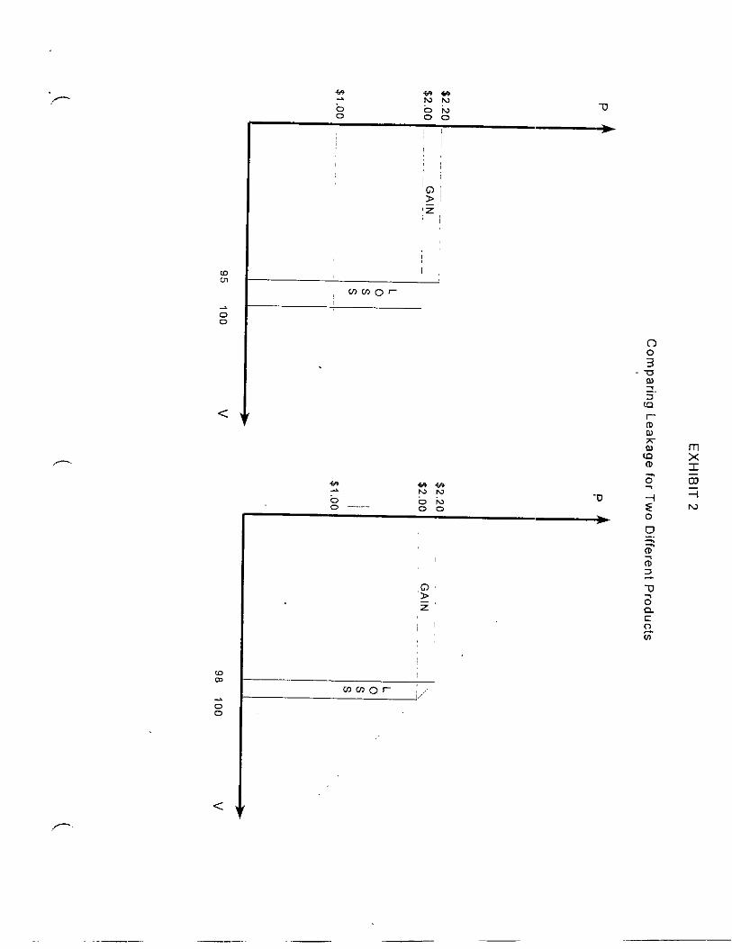
Exhibit 2 presents the demand curves for two postal products, i and j, assumed
for simplicity as linear demand curves. Both products have constant marginal costs of
$1 and the demand equations for postal product i (D,) and product j (DJ are:
vi = 150 - 25.P,
vi = 120 - lO*P;
where P is price of the product in dollars and V is volume demanded at grice P. At a
price of $2, as shown in Exhibit 2, 100 units are demanded of each prodfuct.
According to the above equations, a one dollar increase in the price of product i
causes quantity demanded to decline by 25 units, whereas a one dollar increase in the
price of product j causes quantity demanded to decline by only 10 units. Therefore, the
demand for product i is more price elastic than the demand for postal product j. This
result can also be seen by calculating the elasticities of demand for products i and j.
Recalling the formula for own-price elasticity and noting that in a linear demand
equation the coefficient on price equals AVIAP, the own-price elasticities of demand for
products i and j are equal to
E,; = [AV/v]/[AP/P,] = -25 .P,Ni = -25 *2/l 00 = -0.5
E, = [AV,N,l/[AP/P,l = -10 *P,N, = -10 .2/l 00 = -0.2
Exhibit 2 also shows the net revenues earned by the firm from products i and j,
where net revenue is equal to [P - M].V. With both products having a constant marginal
cost of $1, net revenues from each product are equal to $100 and total net revenues
are equal to $200.
D
,-.
< 1

USPS-T-31 24
Suppose that the combined net revenues from products i and j are insufficient to
cover the common costs of the Postal Service. To raise the required net revenue, the
price of each product is increased from $2 to $2.20. The increase in price (causes a
decline in quantity consumed, with volume falling 5 units to 95 units for product i and
falling 2 units to 98 units for product j. The smaller decline in product j volume reflects
its lower own-price elasticity.
The increase in price from $2 to $2.20 yields an increase in net revenues from
,the units still consumed at the higher price, indicated by the areas. labeled GAIN in
Ex:hibit 2. At the same time, the increase in price causes a partially offsetting decline in
net revenues that were previously earned at the lower price of $2, but are no longer
earned on those units that are not consumed at the higher price of $2.20. This loss of
net revenues is indicated by the areas labeled LOSS in Exhibit 2. The overall change in
net revenues is the difference between GAIN and LOSS. Table 2 mathematically
presents the same information shown in Exhibit 2.
1
2
3
4
5
6
7
8
9
10
11
12
13
14
15 16
17
18
19
20
21
22
23
24
25
26
r Table 2
GAIN and LOSS Resulting from a Price Increase
Product i
Price (P)
t ,
Cost (M) Volume (V) Net Revenue 100 - 25.P (P - M)*V
$2.00 $1 .oo 100 $100.00
t $2.20 1 $1.00 ( 95 $114.00 1
Product j
t
$2.00 $1 .oo 100 $100.00
$2.20 $1 .oo 98 $117.60
Table 2 shows that at a price of $2.20, the net revenue from product i is $114.00,
equal to ($2.20 - $1 .OO) -95, representing a $14.00 increase in the net revenue that was

2
3
4
5
6
7
8
9
10
11
/-- 12
13
14
15
16
17
18
19
20 21 22 23
24
25 26
./-. 27 28
USPS-T-31 25
earned at a price of $2.00. The source of the $14.00 increase is shown as the
difference between a $19.00 GAIN (equal to an additional $0.20 on each of 95 units
consumers) and a $5.00 LOSS (equal to the $1 of net revenue previously earned on
each of 5 units no longer consumed at the higher price).
Table 2 also shows that for product j, net revenue at a price of $2.20 is $117.60.
The $17.60 increase in net revenue is equal to the difference between a $19.60 GAIN
and a $2.00 LOSS.
Note that although the price increases were identical irr the two markets, the
increase in net revenues in market i (GAIN,) is much less tharr the increase in net
revenues in market j (GAIN,). The smaller increase in net revenues in market i is a
direct result of the greater own-price elasticity of product i, which causes a much larger
decline in volume when the price of good i is increased. Exhibit 2, therefore, illustrates
one important aspect of the Ramsey or IER pricing. Raising the price of elastic
products is a less effective method for raising net revenue because the volume of
elastic products declines more as a result of a price increase.
2. GAIN, LOSS and the Leakage Factor k
A measure of the efficiency of raising net revenues is the ratio of the net
revenues lost due to the decline in consumption to the net revenues gained due to the
increase in price. From Table 2, the ratio of LOSS to GAIN is equal to:
Loss= (P - M).AV 64) GAIN V.AP
Multiplying both the numerator and denominator by P and recalling that the own-
price elasticity is equal to [AVr\ll/[APlP] yields,
!LEjS= (P - M).AV P = EYP-M) = -k W) GAIN V.AP P P

1
2
3
4
5
6
I
8
9
10
11
I2
13
14
15
16
17
18
19
20
21
22 23 24 25
26
USPS-T-31 26
which is exactly the expression for the leakage factor k in the IER formula. Thus, the k
value of a product measures the effectiveness of raising additional n’et revenue from
that product.
3. Leakage and the Burden on Consumers
Another way of expressing the efficiency of raising net revenues is to think of the
overall gain in net revenues compared to the burden imposed on consumers. Recall
from Exhibit 1 and Table 1 in Chapter 1 that the burden on consumers from an increase
in price consisted of two areas. The first aspect of the burden consulmers (labeled
AREA 1 in Exhibit 1) is the additional expenditures by consumers at ihe higher price,
identical to the area GAIN in Exhibit 2. The second aspect of the burden on consumers
is the loss net value of those goods not consumers, represented by the triangular AREA
2 in Exhibit I. Although this second aspect of the burden on consumers is important,
AREA 2 will tend to be much smaller than AREA 1, and the loss net value of
consumption is a second-order effect on consumers. Therefore, ignoring this
consideration, the burden on consumers is equal to the additional expenditures for
those goods consumed at the higher price, identical to the GAIN in net revenues shown
in Exhibit 2 and Table 2.
Consequently, one can measure the efficiency of raising net revenues as it
relates to the burden, or the primary aspect of the burden, imposed on consumers.
Recalling that the overall increase in net revenues is equal to GAIN minus LOSS, then
a measure of the overall increase in net revenues per dollar of burden on consumers is:
GAIN - LOSS = 1 - LOSS/GAIN = 1 -k GAIN
Thus, every dollar of burden imposed on consumers yields an overall increase in
net revenues of 1 - k dollars. In turn,, k dollars of net revenue “leak away” from the firm.
-

USPS-T-31 27
1
2
3
4
5
6
7
8
9
10
11
12 ,-
13
14
15
16
17
18
19
20
21
22
23
24
/- 25
4. Desirability of a Constant k Across All1 Products
Exhibit 2 and Table 2 show that the increase in price from $2.00 to $2.20
imposes more leakage from the more elastic product i than thle less elastic product j.
The leakage value for product i, equal to the ratio of LOSS to GAIN is $5.00/$19.00 or
0.26. This means that for each dollar of additional burden imposed on consumers of
product i from the increase in price, 74 cents of additional net revenue is earned, while
26 cents of leakage occurs. In contrast, the leakage value for product j is about 0.16,
equal to $2.00/$19.60, meaning that for each dollar of additional burden on consumers
of product j, about 90 cents of additional net revenue is earned, with only ten cents of
leakage. Note that for both products leakage exists because increases in price lead to
decreases in consumption. But the greater leakage for product i shows that raising the
price of product i is a less efficient (more harmful to consumers) way of capturing an
additional dollar of net revenue for the firm.
Another way of looking at the impact of different levels ‘of leakage is to consider
the change in the burden imposed on consumers associated with raising $1 of
additional net revenues from product j and $1 less of net revenues from product i, so
that total net revenues are unaffected. This change in consumer burden is given by the
difference between the k values for products i and j. Since the k value for product i is
0.26 and the k value of product j increase is 0.10, transferring $1 of net revenues from
product i to product k reduces the burden on consumers by $0.16 (0.26 minus 0.10).
As long as the leakage values for any two products are not equal, the firm could raise
the same total net revenue and lower the burden on consumers by raising the price of
the low leakage product and lowering the price of the high leakage product.
Does this mean that the firm should continue to raise thle price in market j and
lower it in market i ad infinitum? No. As the price in market j is raised, additional price
I.
2
3
4
5
6
7
8
9
10
11
12
13
14
15
16
17
18
19
20
21
22
23
24
USPS-T-31 ~~- 28
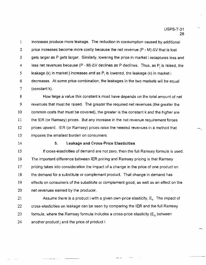
increases produce more leakage. The reduction in consumption caused by additional
price increases become more costly because the net revenue (P - hl).AV that is lost
gets larger as P gets larger. Similarly, lowering the price in market i recaptures less and
less Inet revenues because (P - M).AV declines as P declines. Thus., as P, is raised, the
leakage (k) in market j increases and as Pi is lowered, the leakage (k) in market i
decreases. At some price combination, the leakages in the two markets will be equal
(constant k).
How large a value this constant k must have depends on the total amount of net
revenues that must be raised. The greater the required net revenues (the greater the
common costs that must be covered), the greater is the constant k and the higher are
the IE!R (or Ramsey) prices. But any increase in the net revenue requirement forces
prices upward. IER (or Ramsey) prices raise the needed revenues in a method that
imposes the smallest burden on consumers.
5. Leakage and Cross-Price Elasticities
If cross-elasticities of demand are not zero, then the full Ramsey formula is used.
The important difference between IER pricing and Ramsey pricing is that Ramsey
pricing takes into consideration the impact of a change in the price of one product on
the demand for a substitute or complement product. That change in demand has
effects on consumers of the substitute or complement good, as well ,as an effect on the
net revenues earned by the producer.
Assume there is a product i with a given own-price elasticity, EIii. The impact of
cross-elasticities on leakage can be seen by comparing the IER and the full Ramsey
formula, where the Ramsey formula includes a cross-price elasticity I(E,, between
another product j and the price of product i.

USPS-T-31 29
1
(7A)
2 The tirst term in the Ramsey formula is identical to the IER formula and equals
3 the leakage that results from an increase in the price of product i. The second term in
4 the Ramsey formula can be re-written as shown below by sub:stituting the formula for
5 the cross-price elasticity of product j with respect to the price of product i.
6
7 P.-M. 3 E,i 2 =
?.-PI. ov. Pi -2-J 2-L IL= 'P,Lvj' av,
pi PI v, API Vi v, LiPI (7B)
8
9
10
11
12
13
14
15
The denominator of the second part of the Ramsey formula (Vi-AP,) is the same
as the denominator in the first part of the formula and in the IER formula. It is the GAIN
in revenues resulting from the increase in price of product i. Tlhe numerator of the
second part of the Ramsey formula (P, - M,).AV, is the change in net revenues of
product j that results from the increase in the price of product i,. It is equal to.the net
revenues earned per unit of product j (price of j minus its marginal cost) multiplied by
the change in volume of product j that results from the increase in the price of product i.
If i and j are substitutes, then the increase in the price of product i causes an increase
16 in the volume of product j and an increase in net revenues earned from product j.
17 Therefore, the leakage of net revenue that occurs from the decline in the volume of
18 product i (the first term of the Ramsey formula) is partially offset by an increase in net
19 revenue from the substitute product j. Thus, holding the ownprice elasticity of product i
20 constant, the presence of a substitute product j reduces the leakage caused by an

1
2
3
4
5
6
7
8
9
10
11
12
13
14
15
16
17
18
19
20
21
22
23
24
25
USPS-T-31 30
increase in the price of i. Under Ramsey pricing, products with subslitutes within the
set of products to be priced will have higher mark-ups than products without such
substitutes, assuming the fwo products have the same own-price elasticity
6. Leakage in Competitive and Unregulated Monopoly Markets
Further understanding of the concept of leakage can be gained by examining the
pricing conditions faced by competitive firms and by an unregulated monopolist. As
part olf the analysis, the basic IER pricing equation is re-written in terms of the ratio of
price ,to marginal cost for each product to be priced.
P/M = E/(E + k)
a. Leakage Under Pure Competition
Under pure competition, price equals marginal cost where marginal cost includes
a norrnal profit margin for the firm. A mark-up of price above marginal cost is not
sustainable under pure competition because other firms could set price at marginal cost
and the firm charging the above marginal cost price would see its quantity sold go to
zero. In terms of the above equation, price equals marginal cost when the leakage
factor k is equal to 0. Thus, under perfect competition, there is no leakage.
b. Leakage for an Unregulated Monopoly
Consider now, the pricing strategy for an unregulated profit-maximizing
monopolist. The monopolist will raise prices above marginal costs until the point in
which profits, analogous to net revenues, are maximized. The pricing1 formula for a
profit maximizing monopolist, not derived here but commonly found irr any micro-
‘economics text book is:
P/M = E/(E + 1)
The above formula is identical to the IER pricing formula when the leakage factor
k is equal to 1. Recalling that leakage equals the ratio of net revenues lost to net
-- -

USPS-T-31 31
revenues gained from a price increase, a leakage value of 1 states that a profit-
maximizing monopolist will continue to raise price as long as the price increase loses
less net revenues (or profits) than it gains.
Thus, as prices are increased above marginal cost (the purls competitive
solution), the leakage factor k increases from 0 until (in the unregulated monopoly
solution) it reaches 1. Additional price increases would push the leakage factor above
1, meaning that the price increase would lose more net revenues (profits) than it gains.
Leakage factors of 0 and 1, therefore, form the bounds between the purely competitive
market and the unregulated profit-maximizing monopolist.
.r-.

1
2
3
4
; 8
9
10
11
12
13
14
15
16
17
18
19
20
21
22
23
24
25
26
27
28
29
USPS-T-31 32
Chlapter 3: Data Required for the Calculation of Ramsey Price,s
A. Mail Products Included in Ramsey Price Calculations
The present testimony calculates Ramsey prices for the mail subclasses and
special services presented in Table 3 below.
Table 3 Mail Products Included in the Ramsey Pricing Model
First-Class Letters, Flats. and Parcels
First-Class Cards
Priority Mail
Express Mail
Periodicals In-County Mail
Periodicals Nonprofit Mail
Periodicals Classroom Mail
Periodicals Regular Rate Mail
Standard A Single-Piece Mail
Standard A Regular Mail
Standard A Enhanced Carrier Route
Standard A Nonprofit Mail
Standard A Enhanced Carrier Route Nonprofit Mail
Standard B Parcel Post
Standard B Bound Printed Matter
Standard B Special Rate Mail
Standard B Library Rate Mail
Registry
Insurance
Certified
C.O.D. - Money Orders
-- -~-

1
2
3
4
5
6
7
8
9
10
11
12 /--
13
14
15
16
17
18
19
USPS-T-31 33
Table 3 includes all domestic mail subclasses and special services for which
demand elasticities have been estimated. Included in Table 3 are six preferred
subclasses: Periodicals In-county. Periodicals Nonprofit, Periodicals Classroom,
Standard A Nonprofit, Standard A ECR Nonprofit, and Library mail. Ramsey prices
are not calculated for these mail subclasses. Instead, each of the preferred subclasses
is assigned a mark-up over marginal cost equal to one-half the Ramsey mark-up for the
corresponding regular subclass, following the requirements for the pricing of nonprofit
subclasses set forth in the Revenue Forgone Reform Act. However, because the
nonprofit subclasses yield net revenues and help satisfy the break-even requirement,
they are included in the Ramsey pricing model even though their prices are
constrained.
The Ramsey pricing formula, reprinted below, shows that in order to calculate
Ramsey prices, information is needed on marginal costs (M,), price elasticities (E,,), and
volumes (Vi and V,) of each subclass or special service. In addition, a break-even
revenue requirement, which determines the value of the leaka!ge factor k, must be
satisfied. The present chapter discusses each of these necessary inputs as they relate
to the calculation of Ramsey prices of postal products.
C.1)
20 B. Own-Price and Cross-Price Elasticities
21 1. Elasticities Used in Ramsey Price Calculations
22 Ramsey prices depend on own- and cross-price elasticities of demand. The _I---
23 price elasticit,ies used in the Ramsey price calculations are the long-run price elasticities

1
2
3
4
5
6
7
8
9
10
11
12
13
14
15
16
17
18
19
20
21
22,
23
24
25
USPST-31 34
presented in this case by Mr. Thress (USPS-T-7), and Dr. Musgrave (USPS-T- 8) for
Priority and Express Mail. These elasticities are obtained from volume demand
equations estimated using quarterly data. Included in the set of explanatory variables
are the real price paid by the mailer in the current quarter and three lagged postal
quarters. The inclusion of price lags in the demand equation reflects the fact that mailer
response to a change in postal rates occurs over a period of time. The price elasticities
used in the Ramsey price formula are the long-run price elasticities equal to the sum of
the current, and three lagged elasticities.
In the econometric estimation of the price elasticities of First-Class letters and
cards, and Standard A Regular and Nonprofit mail, price is measured as postage price
plus user costs. User costs are costs borne by the mailer to satisfy worksharing
requirements. The estimated price elasticity is the percentage change in volume
associated with a one percent change in price including user cost. To be consistent
with the demand elasticities estimated for these subclasses, the Ramsey price is the
Ramsey postage price plus user costs. The Ramsey price reported in this. testimony,
however, is the Ramsey postage price obtained by subtracting the user cost from the
Ramsey price including user costs.
LR-H-164 shows that measuring the Ramsey price with user costs iis necessary
to maintain consistency with the demand elasticities of mail products that include user
costs. LR-H-164 presents the Ramsey price calculation for Standard A Regular mail
and shows how the Ramsey postage price is obtained from the Ramsey price. It is
worth noting that the impact of user costs on the Ramsey postage prices i!: quite small.
2. Subclass Elasticities for First-Class Letters and Ciards
Ramisey prices are calculated for mail subclasses and special services. The
Postal Service demand equations include two subclasses in which separa,te elasticities

1
2
3
4
5
6
1
8
9 10 11 12
13 /--
14
15
16
17 18 19 20 21 22 23
24
25
26
27
28 29
/- 30
USPS-T-31 35
are estimated for categories within the subclass. Separate demand equations are
estimated for single-piece and workshared (presorted or automated) letters within the
First-Class letter subclass and for stamped postal cards and private postal cards within
the First-Class cards subclass. In order to calculate Ramsey prices for the First-Class
letter and First-Class card subclasses, elasticities for each sulbclass are estimated by
taking a volume weighted average of the separate elasticities of the two components of
the subclass. The volumes used in calculating the weights are the before-rates Test
Year volumes. Tables 4 and 5 shows estimated subclass elasticities for First-Class
letters and cards, respectively. The calculations are presentsfd as part of LR-H-165.
Table 4 Estimated Price Elasticities for the First-Class Letter Subclass
Category Test Year Volume Own-Price Volume Weight Elasticity
single-piece 54,394.309 0.5672 -0.189240
workshared 41,506.989 0.4328 -0.269173
total letters 95,901.297 1 .oooo -0.232492
Cross-price elasticity 1 is the estimated elasticity with respect to the price of the First- Class card subclass. Cross-price elasticity 2 is the estimated cross-elasticity with respect to the price of Standard A Regular mail.
Table 5 Estimated Price Elasticities for the First-Class C:ards Subclass
Category Test Year Volume Volume Weight
stamped 594.894 0.1045
private 5,098.223 0.8955
total cards 5,693.117 1 .oooo
Cross-Elasticity 1 is the estimated cross-elasticity with respect to First-Class letters.
__--. -.

1
2
3
4
5
6
7
8
9
IO
11
12
13
14
15
16
USPS-T-31 - 36
Table 4 shows that based on the estimated elasticities and the forecasted
before-rates Test Year volumes, the own-price elasticity of the First-Class letter
subclass i,s estimated to be -0.232492, the cross-price elasticity between letters and the
price of Fi,rst-Class cards is estimated to be 0.005522 and the cross-price elasticity
between letters and the price of Standard A Regular mail is estimated to Ibe 0.025925.
Table 5 shows that the own-price elasticity of the First-Class cards subclass is
estimated to be -0.862674 and the cross-price elasticity between cards and the price of
First-Class letters is estimated to be 0.176007.
Not’e an estimated discount elasticity exists between the single-piece and
workshared letters to measure shifts of mail between these two categoric:; in response
to a change in worksharing discounts. Ramsey prices are calculated as a~ subclass
level and worksharing discounts are subsumed in the overall price of the subclass.
Thus, the estimated discount elasticity is not needed here.
Table 6 presents a complete list of the own- and cross-price elastic,ities used in
the calculation of the Ramsey prices presented in this testimony.

USPS-T-31 37
1 2
3
4 First-Class Letters
8
9
10
11 ,f-
12
13
14
15
16
17
18
19
20
21
22
23
24
./-- 25
Mail Product
First-Class Cards
Priority Mail
Table 6 Estimated Price Elasticities
Own-Price Elasticity
Cross-Price Elasticity Cross-Price Elasticity
-0.662674 0.176007 (First-Class letters)
Express Mail
Periodicals In-County
Periodicals Nonprofit -0.227917 I
Periodicals Classroom -1.178481
Standard A ECR 1 -0.597746 1
Standard B Bound Printed 1 -0.335170 1
Standard B Special Rate -0.362037
Standard 6 Library Rate -0.634333
Registry -0.413445
Insurance -0.104734
Certified -0.286961
C.O.D. -0. I 82012
Money Orders -0.391377 -L----l
1
2
3
4
5
6
J
8
9
10
11
12
1.3
1.4
15
16
17
18
19
2.0
2,l
22
23
24
USPS-T-31 - 38
C. Marginal Costs
The Ramsey pricing formula requires product marginal cost;. Ramsey prices
are calculated for a 1998 Test Year and use forecasts of Test Year cost, including the
one percent contingency. The marginal cost of a product, as it is strictly defined in
economics, is the additional cost associated with a one unit increase in output of that
product. The Postal Service costing methodology provides a cost (estimate that is
similar to marginal cost, known as volume variable cost. Volume variable cost is
defined as those costs of a mail product that vary with volume. Product marginal costs
for 1998 are taken as equal to per piece volume variable costs, calculated by dividing
Test Year before-rates volume variable cost by Test Year before-rates volume, as
presented in Mr. Patelunas’s testimony (USPS-T-15). It is assum’ed that in the range
of volumes being considered, volume variable cost per piece, and therefore marginal
cost, is constant for every mail product.
As noted in the previous section, the prices of First-Class letters and c.ards, and
Standard A Regular and Nonprofit mail are measured including user costs. To be
consistent with this price measure, the marginal costs of these mail products is
measured as the sum of the volume variable cost per piece and the mailer user cost, or
the total (Postal Service plus mailer) cost per piece.
Another cost measure that should be considered in rate-making is incr-emental
cost. The incremental cost of a product is the cost that the Postal Service would save
if thse product were eliminated entirely. In addition to covering the products volume
variiable costs, postal prices (Ramsey or otherwise) should generate sufficient revenues
to cover the product’s incremental cost. If not, the Postal Service and mailers would be
better off if the product were discontinued.
-

P USPS-T-31 39
Accordingly, Ramsey prices are calculated as a mark-up over marginal cost. The
total revenues from the product at the Ramsey prices are therl compared to the
product’s incremental cost. If these total revenues are less than incremental cost, the
price must be marked up above the Ramsey price until revenues cover incremental
costs. As it turns out, Express Mail and Registry mail have Ramsey prices that
generate revenues below incremental costs. Consequently, the prices of these two
products are constrained above their Ramsey prices so that revenues cover
incremental costs.
Table 7 shows 1998 Test Year forecasted before-rates volume, volume variable
costs, volume variable costs per piece (taken to be marginal cost excluding user costs),
and incremental costs for the 22 products included in the Ramsey price model. Costs
include the one percent contingency.
1
2
3
4
5
6
7
8
9
10
11
12 /-

USPST-31 40
6
7
8
9
10
II
12
13
14
15
16
ll
18
19
20
21
22
23
24
25
26,
21
28
29
Table 7 Cost Data for 1998 Test Year
1
2
3
4
5
6
I
8
9
10
11
12 /--
13
14
15
16
17
18
19
20
21
22
23
24
25 ,--
USPS-T-31 41
D. Volume Forecasts
Forecasted volumes are needed in the calculation of the Ramsey prices, as the
Ramsey price of a mail subclass depends on its volume and on the volumes of any
other subclass with which it has a cross-price elasticity. Forecasted volumes are also
needed to calculate total revenues and total costs and deterrnine if the break-even
requirement is satisfied.
1. Volume Forecast Methodology
The starting point of, the forecasted Test Year volumes at the Ramsey prices are
the forecasted Test Year volumes at current postal prices, known as the before-rates
volume forecast. The before-rates forecast of mail volumes is presented in the
testimony of Dr. Tolley (USPS-T-6), and include the before-rates forecasts of Priority
and Express Mail also presented in the testimony of Dr. Musglrave (USPS-T-8). Both
Dr. Tolley and Dr. Musgrave use the same forecasting approach, which involves
projecting the Test Year volume from the volume in a Base Yefar through the use of a
series of projection factor multipliers. Each projection factor considers the impact of a
particular variable (e.g., price, income, or population) on volume from the Base Year to
the Test Year.
The same basic approach is used to project volumes in the Test Year at the
Ramsey prices. The Test Year Ramsey volume is projected from the Test Year
before-rates volume through the use of a projection factors. Because the Test Year for
the Ramsey volumes is the same as the Test Year for the before-rates volumes, the
only variable which differs between the two forecasts is the postal price. Therefore, the
Ramsey Test Year volume of a mail product is obtained by mu~ltiplying the before-rates
Test Year volume of the product by a projection factor which accounts for the change in
the price of the mail product. If the volume of the product depends on the price of other
-

USPS-T-31 42
postal products, a cross-price projection factor multiplier is also included in the volume
forecast at the Ramsey prices.
The price projection factor multiplier is equal to the ratio of the Ramsey price to
the before-rates price raised to the estimated price elasticity. In a simplified form and
without cross-price elasticities, the Ramsey volume forecast can be presented as:
Ramsey Volume = Before-Rates Volume . (PR/P,JE
where P, is the Ramsey price of the subclass, P,, is the before-ratses price of the
subclass, and E is the estimated own-price elasticity of the subclass. (PR/PbJE is known
as the rate projection factor multiplier. Prices include user costs, where appropriate.
2. Elasticities Used in the Test Year Volume Forecasts
The simplified form of the rate projection factor multiplier differs from the rate
projection factor multipliers used is the forecasts of Drs. Tolley and1 Musgrave. In
particular, the forecasts of Drs. Tolley and Musgrave are made on a quarterly basis,
using the current and three lagged price elasticities and including terms that convert the
annual Base Year volume into a quarterly volume. Moreover, forecasted quarterly
volumes are converted into an annual volume for the Test Year, which does not begin
at tlhe beginning of a postal quarter. This exact approach differs from the approach
described above for the Ramsey volume forecasts in which a singIl? rate projection
multiplier is used to convert the before-rates Test Year volume into a Ramsey Test Year
volume while the full volume forecasting approach uses four rate projection tactor
multipliers, one for each of the current and three lagged estimated elasticities. Current
and lagged elasticities are included in the volume forecasts because the econometric
eviclence shows that mailers response to a change in postal rates does not all occur in
the,quarter in which rates were changed. The lagged elasticities reflect the period of
1
2
3
4
5
6
7
8
9
10
11
12
13
14
15
16
17
18
19
20
21
22
23
24
-,

1
2
3
4
5
6
7
8
9
10
11
12 I-.
13
14
15
16
17
18
19
20
21
22
23
24
25 ,-
USPS-T-31 43
adjustment by mailers to the new rates. In the long-run, the volume response is given
by the sum of the current and lagged price elasticities.
For the present rate case, the new rates are assumed to be put in effect on the
first day of the Test Year. The volume impact in the first quarter following the rate
increase will be smaller than the impact in the fourth quarter following the rate increase,
owing to the lagged response of mailers to changes in rates as measured by the current
and lagged price elasticities. Consequently, the volume response in the Test Year is
not the long-run response and using the long-run elasticity to forecast the Ramsey Test
Year volumes would overstate the volume impact of the change from the before-rates
price to the Ramsey prices.
One solution to this problem would be to use the full volume forecasting
approach including current and lagged elasticities and seasonal coefficie!nts to make
the Ramsey volume forecasts on a quarterly basis instead of making Test Year
forecasts using a single elasticity. However, the Ramsey price computer calculations
require an iterative approach, necessitating frequent calculations of volulne, revenues,
and costs, and use of the full forecast methodology employed by Drs. Tolley and
Musgrave was considered impractical. Instead, effective Test Year elasticities are
used where the effective Test Year elasticity is a weighted aver-age of the estimated
current and lagged elasticities. For example, in the first quarter of the Test Year, only
the current elasticity affects mail volume. In the second quarter, the current and first
lagged elasticity affect mail volume, in the third quarter the current and first two lagged
elasticities affect mail volume, and in the fourth quarter of the lest Year, the current
and all three lagged elasticities affect mail volume. The effective elasticity for the Test
Year, bearing in mind that the first three postal quarters are 12 weeks long while the
fourth postal quarter is 16 weeks long is calculated as:

USPS-T-31 44
1 2 3 4 5
6
7
8
9
10
11
12
13
:14
15
16
I!7
118
I,9
20
21
22
23
24
25
26
27
(12/52)*(current elasticity) + (12/52)*(current elasticity + lag 1 elasticity) + (12/52)*(current elasticity + lag 1 elasticity + lag 2 elasticity)’ + (16/52)*(current elasticity f lag 1 elasticity + lag 2 elasticity + lag 3 elasticity) As an example, the effective Test Year own-price elasticity of Standard A
Enhanced Carrier Route mail is calculated below. LR-H-165 presents the entire set of
effective Test Year price elasticities used in making the Ramsey volume forecasts.
Effective Test Year elasticity for Standard A ECR Mail =
(12/52)*(-0.223143) +
(12/52)*(-0.223143 - 0.154656) +
(12/52)*(-0.223143 - 0.154656 - 0.114297) +
(16/52)*(-0.223143 - 0.154656 - 0.114297 - 0.105650) =
-0.436161
Thus, the effective own-price elasticity for Standard A ECR rvlail in the Test Year,
assuming that after-rates prices take effect on the first day of the Test Year, is -0.436. ,,, ., I
This elasticity is less than the long-run own-price elasticity of Standard A ECR mail of
-0.598 because the full impact of the new rates is not entirely reakzed in the Test Year.
As a check, the Ramsey volume forecasts presented in this testimony were
compared to full volume forecasts (using the Ramsey prices and complete lag structure
of price elasticities) for the 1998 Test Year. The Ramsey volume forecasts ffcr.every
subclass were always within one-half of one percent from the forecasts obtained using
the full volume forecasting methodology. For many mail products, ,the difference in
volume forecasts was on the order of one-tenth of one percent. ThIe impact Ion
forecasted revenues and costs was of the same order of magnitude and the impact on
net revenues was even smaller.
-

USPS-T-31 45
E. Ramsey Net Revenue Requirement
1. Defining the Ramsey Net Revenue Requirernent
The Ramsey prices must generate projected Test Year revenues equal to
projected Test Year costs. Test Year revenues and costs include revenues and costs
generated from the products included in the Ramsey pricing model as well as revenues
and costs generated from other Postal Service operations.
Some revenues and costs are unaffected by the Ramsey prices presented in this
testimony. Product specific fixed costs and other non-volume variable costs are not
affected by the Ramsey prices or volumes. In addition, the revenues and costs of
products not included in the Ramsey pricing model, as well as reve,nues from
investment income and a small congressional appropriation for such things as free-for-
the-blind mail are not affected by the Ramsey prices. The Ramsey net revenue
requirement is defined as the excess of total revenues over total volume variable costs
of the products included in the Ramsey pricing model that is necessary to yield total
Postal Service revenues equal to total Postal Service costs in the Test Year.
Table 8 shows the various components of Test Year revenues and costs that are
unaifected by the Ramsey prices of the products considered in this testimony.
1
2
3
4
5
6
7
8
9
10
11
12 .-.
13
14
15
16
17
18 19
20 21
22 23
24 25
26 I---
2’7
Table 8
- Revenues and Costs Not Affected by Ramsey Pricing
Non-Ramsey Revenue or Cost Source
-- NoIn-Volume Variable CO!stS
Test Year Projected Revenues
(in $millions)
Test Year Projected Costs
(in $millions)
26.719.265
Products not included in Ramsey pricing model
- Other Income
2,659.X36
254.311
2,045.061
-4
Total - 2,914.097 28,764.326

USPS-T-31 -.-. 46
Among the products not included in the Ramsey priing model are Mailgrams,
Free-for-the-Blind mail, International Mail, Stamped Envelopes, Special Handling, and
PI). Boxes.
Table 8 shows that the Postal Service has projected Test Year revenues of
2,914 million dollars and projected Test Year costs of 28,764 million that are unaffected
by the Ramsey prices presented in this testimony. The difference between these
projected revenues and costs is 25,850 million dollars. Therefore, the products
included in the Ramsey pricing model will need to generate 25,850 million dollars of net
revenue (total revenue less total volume variable costs) to yield total Postal Service
revenues equal to total Postal Service costs.
It should be recognized that this revenue requirement is estimated for hte
purposes of establishing a target for this Ramsey pricing exercise and does not
necessarily match the revenue requirement used by the Postal Service in their
proposed rates.
2. Calculating Ramsey Net Revenues
For each mail product subject to Ramsey pricing, product net revenue is defined
as t,he difference between product revenues and product volume variable costs.
Product revenue at the Ramsey price is calculated as the Ramsey price multiplied by
the Ramsey volume. In other words, the Ramsey price is taken as a measure of
average revenue per piece. Similarly, product cost is calculated as volume variable
cost, per piece (or marginal cost) multiplied by product volume at the Ramsey price.
Thus, the Ramsey prices satisfy the break-even condition if:
Ramsey Net Revenues = x[(PR .V,) - (MC,.V,)] = $25,850 million
= r[(PR - MC&V,] = $25,850 million
-.
1
2
3
4
5
6
7
8
9
10
11
12
13
14
15
16
17
18
19
20
21
22
23
24
25

.-
1
2
3
4
5
6
7
8
9
10
11
12 /-.
13
14
15
16
17
18
19
20
21
22
23
24
,/- 25
USPS-T-31 47
It is important to note that the forecasted volume is based on the ratio of the
Ramsey to the before-rates price of the mail product, where both the Ramsey and the
before-rates prices include estimated user costs for First-Class and Standard A mail
subclasses. User costs, however, do not provide revenue to t,he Postal Service.
However, since user costs are included in both the price and marginal cost measures
for these mail products. the difference between price and marginal cost is the same
whether both are measured with user costs or both are measured Without user costs.
F. Price Constraints
1. Incremental Cost Coverage
In addition to covering the product’s volume variable cclsts, postal prices should
generate sufficient revenues to cover the products incremental cost. If not, the Postal
Service and mailers would be better off if the product were discontinued. The Ramsey
price of Express Mail and of Registry mail, while above the product’s marginal cost, are
not sufficiently above marginal cost to also cover the products incremental costs.
Therefore, the prices presented for these products are not the Ramsey prices but a
higher price that provides sufficient revenue above volume variable cost to also cover
incremental cost.
2. Preferred Subclasses
As a requirement of Revenue Forgone Reform Act, the mark-up for preferred
subclasses of mail is set at one-half the mark-up of the corresponding regular subclass.
The six preferred subclasses are Periodicals In-county, Nonprofit, and Classroom mail,
Standard A Nonprofit and Nonprofit Enhanced Carrier Route, and Standard B Library
rate. The three preferred subclasses of Periodicals mail are assigned a mark-up equal
to one-half the mark-up on Periodicals Regular mail; Standard A Nonprofit and
Nonprofit Enhanced Carrier Route are assigned mark-ups equal to one-half the mark-

USPS-T-31 48
1 ups for Standard A Regular and Enhanced Carrier Route mail, respectively; and Library
2 Rate is assigned a mark-up equal to one-half the mark-up on special rate.
3
4
5
6
7

USPS-T-31 49
1
2
3
4
5
6
7
8
9
10
11
12 /-
13
14
15
16
17
18
19
20
21
22
23
24
/-- 25
Chapter 4: Non-Ramsey After-Rates Prices for R97-1
A. Why Non-Ramsey Prices are Needed
The benefits from Ramsey pricing can be measured in comparison to some
other rate schedule that also satisfies the Postal Service’s break-even requirement. In
this testimony, the Ramsey prices are compared to an illustraiive break-even rate
schedule based on the Postal Rate Commission’s (PRC) reco’mmended mark-ups in
R94-1, applied to 1998 Test Year costs and adjusted to satisfy the Ramsey net revenue
requirement of $25,850 million. In this way, the Postal Service’s net financial position is
unaffected by whether the Ramsey or non-Ramsey rate schedule is employed. The
benefit to mailers from the move to Ramsey pricing from the non-Ramsey rate schedule
represents a pure gains to mailers that does not come at the expense of the Postal
Service.
B. Non-Ramsey Rates Based on Commission’s IR94-1 Rates
1. R94-1 Mark-Ups
The starting point for the calculation of the non-Ramsey prices for the 1998 Test
Year is the R94-1 rate schedule. Table 9 below presents the lR94-1 recommended
mark-ups, defined as the excess of product revenue over product attributable cost, for
the products included in the Ramsey price model, obtained from Appendix G, Schedule
3 of the Postal Rate Commission’s R94-1 Opinion and Recommended Decision and
Appendix J. Table 9 shows the system-wide mark-up, equal to total revenues from mail
and special services less total attributable costs, divided by total attributable costs.
Table 9 also shows the mark-up index of each mail sublslass, calculated as the
ratio of subclass mark-up to system wide mark-up. For example, the R94-1
recommended mark-up of First-Class letters is 74.5, meaning that at recommend rates,
projected revenues from First-Class letters are 74.5 percent greater than projected

1
2
3
4
5
6
I
8
9
10
11
12
13
14
15
16
17
18
19
USPS-T.-31 - 50
attributable costs. The system wide mark-up is equal to 56.8. Therefore, the relative
mark-up of liirst-Class letters is equal to 74.5/56.8 or 1.31. Similar, calculations yield
the relative cost coverages of the other products included in the Ramsey price model.
2. R94-1 Mark-ups Applied to Test Year Marginal Cosls
The 1194-l mark-ups are applied to 1998 Test Year marginal (volum’e variable
per piece) c:osts to yield a set of prices. Some modifications are required. First, the
R94-1 mark:-ups are mark-ups over attributable cost which for most mail products is
virtually identical to volume variable costs. For some products, Express Mail of
particular importance, attributable costs exceed volume variable costs significantly
because of a substantial level of specific fixed costs. Therefore, the R94-1 mark-up,
which measures the mark-up over attributable costs, is adjusted to measure the mark-
top over vollume variable costs. Second, for the six preferred subclasses, tlie mark-up
over marginal cost is set equal to one-half the mark-up of the corresponding regular
subclass.
After including the above modifications, the volumes of each mail SUbclaSS and
special service are forecasted using the effective Test Year price elasticities presented
earlier. From the volume forecasts, total revenues and total costs are calc,ulated.
Applying thie R94-1 mark-ups to 1998 Test Year costs yields net revenues less than the
net revenue requirement of $25,850 million.
-- ._-

r” USPS-T-31
Table 9 R94-1 Mark-Ups of Mail Products Included in the Ramse Pricin Model
Subclass or Special Service
1 E;;oecommended ‘&I
1 2
3 4
5
6
7
8
9
10
11
12
13
14 15
z’: 22
23
24
25
26
21
28
29
30
31
I - First Class Letters, Flats, and Parcels I
First-Class Cards
Priority Mail
Express Mail
Second-Class In-County Mail
Second-Class Nonprofit Mail
Second-Class Classroom Mail I 6.6 t 0.119 --1 Second-Class Regular Rate Mail
Third-Class Single-Piece Mail
Third-Class Sulk Regular Carrier-Route Mail I
Third-Class Bulk Nonprofit Noncarrier- Route Mail
Third-Class Bulk Nonprofit Carrier-Route Mail
Fourth-Class Parcel Post
Fourth-Class Bound Printed Matter I
Fourth-Class Special Rate Mail
Fourth-Class Library Rate Mail 0.8
Registry 44.5
Insurance 39.8
Certified 70.2
Monev Orders
All Mail and Special Services
32 ,-- 33
--__~ -.-~ .--
IJSPS-T-31 -. 52
1
2
3
4
5
6
7
8
9
10
11
12:
13
14,
15
16
17
18
19
20
21
22
23
24
One reason why the net revenues obtained from the R94-1 mark-ups are less
than the Ramsey net revenue requirement of 25,850 million dollars is that the costing
methodology for the current case results in more non-volume variable costs and less
volume variable cost than the methodology used in R94-1. Therefore, the mark-up of
price over volume variable cost per piece will have to be greater for the current case
than in R94-1. To maintain the relative levels of the R94-1 mark-ups, the R94-1 mark-
ups of each postal product are increased proportionally until total net revenues are
25,850 million dollars. The net revenue requirement is satisfied when the mark-up of
each product is increased 33.7 percent. Note that this does not imply that prices are
increased 33.7 percent because the higher mark-up is applied to geinerally lower costs
per piece.
3. Presentation of Non-Ramsey Test Year Mark-ups
Table 10 presents the break-even non-Ramsey mark-ups for a 1998 Test Year,
Table 10 shows the mark-up indexes of each product are approximately equal to the
mark-up indexes in R94-1. The indexes are not exactly equal because the R94-1 mark-
up index was relative to all mail and special services and the index presented in Table
10 is a mark-up relative to the overall mark-up of the products included in the Ramsey
model. Moreover, the nonprofit subclasses have been assigned relatively higher mark-
ups than in the R94-1 case, which causes their mark-up index to be higher and the
mark-up indexes of the other mail products to be lower than in R94-I. Still, the relative
markups between any two products is the same as in R94-I For example, in R94-1,
the mark-up for First-Class letters was 74.5 or 2.03 times the mark-up on First-Class
cards of 36.7, For R97-1, the mark-up for First-Class letters is 99.65, also equal to 2.03
times the R97-1 mark-up for First-Class cards of 49.09.
-,

1
2
:
5
6
7
8
9
10
11
12
13
14
15 /-
16
17
18
19
20
21
22
23
24
25
26
21 28
29
30
,-- 31
USPS-T-31 53
Table 10 R97-1 Mark-Ups for the Non-Ramsey Rate Schedule
Subclass or Special Service
R97-1 Mark-up I
R97-1 Mark-Up Index
First-Class Letters, Flats, and Parcels
First-Class Cards 49.09 ] 0.613 1
Priority Mail
Express Mail
Second-Class In-Countv Mail
Second-Class Nonprofit Mail
Second-Class Classroom Mail 10.90 0.136 I
Second-Class Regular Rate Mail
Third-Class Single-Piece Mail
Third-Class Bulk Regular NCR Mail
Third-Class Bulk Regular CR Mail
Third-Class Bulk Nonprofit NCR Mail
Third-Class Bulk Nonprofit CR Mail
Fourth-Class Parcel Post 10.03
Fourth-Class Bound Printed Matter
Fourth-Class Soecial Rate Mail
Fourth-Class Library Rate Mail 3.08 1 0.038 t Registry Mail
Insurance
Certified
COD
Money Orders
Overall Mark-up on Above Products
Note that the mark-up on Express Mail is a mark-up over marginal (volume variable)
cost and is not directly comparable to the R94-1 mark-up of price over attributable cost
per piece.

USPS-T-31 - y. 54
1
2
3
4
5
6
7
8
9
10
11
12
13
14
15
16
17
18
19
20
21
22
23
24
25
Chapter 5: Ramsey Prices for R97-I
A. Aggregate Results
1. Description of Table
Table 11 presents a comparison of Ramsey and the non-Ramsey rate schedule
presented above. The first section of Table 11 presents three columns of general
information about each of the 22 subclasses and special services that comprise the
model: name, R97-1 estimated elasticity and marginal costs, equal to volume variable
cost per piece. The 22 mail products are grouped by class: First-Class Iletters and
cards, th’e two expedited mail subclasses, Priority Mail and Express Mail, the four
Periodicals subclasses, the five subclasses of Standard A mail, the four subclasses of
Standard! B mail, and five special services.
The middle section of Table 11 presents the non-Ramsey after-rates price based
on the m,ark-ups presented in Table IO. the mark-up of price over margilnal cost, after-
rates volume (in millions of pieces), product revenues, volume variable costs and net
revenues,. For example, First-Class letters has a non-Ramsey after-rates postage price
of $0.3488, measured as a fixed weight index price, yielding a mark-up of 99.65 percent
over Test Year volume variable cost per piece of $0.1747. Forecasted after-rates
volume is; 95,369 million pieces, generating revenues of $33,263 million, volume
variable costs of $16,661 million, and net revenues of $16,603 million.
,-
The bottom row of the middle section of Table 11 presents total vmolumes,
revenues, volume variable costs, and net revenues for the non-Ramsey rate schedule.
Total volume (not including the special services) is 193,400 million pieces. Total
revenue from the 22 mail products is $58,133, with total volume variable costs of
$32,283 million, yielding net revenues of 25,850 million, thereby satisfying the break-
even requirement for these mail products. The overall mark-up for the non-Ramsey

i i
I “O!,,!W CZO’LB = 6U!3!Jd hasluey “ml sla,!el”l 0, “!eE) ~a,BW!,s3

2
3
4
5
6
7
8
9
10
11
1.2
13
14
15
16
17
18
19
20
21
22
23
24
25
USPS-T-31 56
_...
prices, equal to total revenues less total volume variable costs, divided by total volume
variable costs, is 80.07 percent.
The third section of Table 11 presents Ramsey price information following the
same organization as the non-Ramsey section. The Ramsey price, mark-up, volume,
revenue, and volume variable cost of each product are given. The bottom of the
section shows total forecasted Test Year mail volume under Ramsey pricing of 202,117
million pieces or 4.5 percent more than the non-Ramsey volume. Total revenue under
Ramsey pricing is equal to $59,077 million and total volume variable Cost is 33,227
million. Net revenues under Ramsey pricing are $25,850 million whiczh satisfies the
Ramsey net revenue requirement. The average mark-up under Ram:sey pricing is
77.80 percent.
The increase in total mail volume and the decrease in average mark-up are a
reflection of the benefit to mailers from Ramsey pricing. A more form;al presentation of
this benefit is the increase in consumer surplus under Ramsey pricing1 as opposed to
the non-Ramsey rate schedule. Table 11 shows that the increase in (consumer surplus
from Ramsey pricing is $1,023 million in the Test Year. Chapter 6 discusses the
increalse in consumer surplus from Ramsey pricing in more detail.
2. Summary of Key Differences in Prices
In general, products that have a relatively low own-price elastic:ity have a higher
Ramsey mark-up than non-Ramsey mark-up. This is the case for First-Class letters,
Periodicals Regular rate, and Standard A Regular mail. Conversely, products that have
a relatively high own-price elasticity have lower Ramsey mark-ups tha,n non-Ramsey
mark-ups, e.g., First-Class cards, Priority and Express Mail, and Standard A ECR Mail.
Of particular interest, is the relative mark-ups for Standard A Regular and
Standard A ECR mail. Under the rates based on the R94-1 rates, Staridard A Regular
---.
---

/-
1
2
3
4
5
6
7
8
9
10
11
12 r
13
14
15
16
17
18
19
20
21
22
23
24
USPS-T-31 57
mail has a mark-up of 32 percent and Standard A ECR has a mark-up of 144 percent.
Under Ramsey pricing, the relatively less elastic Regular mail has a mark-up of 79
percent while the relatively more elastic ECR mail has a mark-up of 20 percent.
Overall, the five subclasses of Standard A mail (including single-piece and Nonprofit
mail) generate $4,710 million of net revenue under Ramsey pricing and $4,909 million
under the non-Ramsey rate schedule. The net revenues are about four percent less
under Ramsey pricing, showing that the main effect is to change the relative pricing and
relative contributions to net revenue from Regular and ECR mail.
3. Non-Ramsey and Ramsey Mark-up Indexes
Table 12 compares the mark-up index of each mail product under the non-
Ramsey and Ramsey rate schedules. The mark-up index is equal to the product mark-
up divided by the overall mark-up of the 22 mail products included in the Ramsey
model. For example, the non-Ramsey mark-up of First-Class letters is 99.65 percent as
compared-with a overall mark-up of 80.07 percent. Thus, the mark-up index for letters
is 1.244 (99.6Y80.07) meaning that the mark-up on letters is ‘I ,244 times the average
mark-up. The Ramsey mark-up of First-Class letters is 103.29 percent as compared to
an overall Ramsey mark-up of 77.80 percent. The mark-up index for letters under
Ramsey pricing is 1.328 (103.29/777.80). This result shows that although the mark-up of
letters under Ramsey pricing is only slightly more than the mark-up under non-Ramsey
pricing (103.29 percent vs. 99.65 percent), the relative mark-up of letters is
meaningfully greater under Ramsey pricing (1.328 vs. 1.244). This occurs because by
raising net revenue more efficiently, Ramsey pricing produces a lower overall mark-up
for the 22 products included in the model.

USPS-T-31 -' 58
:
3
4
5
7
8
9
I,0
I. 1
1.2
13
14
15
16
17
18
19
20
21
22
23
24
25
26 27
28
TABLE 12
r M,ail Product
Mark-Up Comparison
Non-Ramsey Non-Ramsey Mark-up Mark-up Index
1 Ramst;i/fl
1 First-Class Letters 1
First-Class Cards 49.09 0.613
130.01 1.624
113.03 1.412
1 Periodicals In-County
Periodicals Nonprofit
t Pwiodicals Classroom
Regular
Standard Single Piece
21.80
6.02
Standard Regular
t Standard ECR
31.97
144.12
Standard Nonprofit 15.98 0.200
Standard NP ECR 72.03 0.900
10.03 0.125
Bound Printed Matter
Special Rate
t Registry Lib’rary Insurance - Rate 59.52 53.24 3.08 0.038 0.743 0.665
1 Certified 93.91 I 1.173 I 53.49 I 0.688 I COD
t
-
Money Orders
3.61 0.045
15.11 0.189
L Overall 80.07 1.000 77.8 1 1.000 1
1
2
3
4
5
6
7
8
9
10
11
12 /-
13
14
15
16
17
18
19
20
21
22
23
24
,/- 25
USPS-T-31 59
B. Individual Subclass Results
1. First-Class Letters
The Ramsey price of First-Class letters is $0.3551, 0.63 cents more than the
non-Ramsey price of $0.3488, and 1.31 cents more than the before-rates price of
$0.3420. Recall that this price is a fixed-weight index price and does not refer to the
price of the basic one ounce letter, currently priced at 32 cents. The higher Ramsey
price is a direct result of the relatively low own-price elasticity of First-Class letters and
the fact that letters are a substitute for two other postal produicts, First-Class cards and
Standard Regular mail. Thus, raising the price of letters is a relatively efficient way to
raise net revenue, first because the higher price causes a small decline in volume due
to the low own-price elasticity and because the higher letters price causes increases in
net revenues earned from an increase in the volume of its two substitute postal
products.
The Ramsey volume of First-Class letters is 95,526 million pieces, actually
somewhat greater than the non-Ramsey volume of 95,369 milllion pieces. The higher
volume occurs despite the higher price because the higher price of Standard Regular
mail under Ramsey pricing causes an increase in the volume of letters. Again this
shows that raising the price of First-Class letters (and Standard Regular mail) is an
effective way to raise net revenue because little overall volume is lost. Total net
revenues under Ramsey pricing is $17,237 million, about $634 million more than under
the non-Ramsey rate schedule.
2. First-Class Cards
The Ramsey First-Class cards price is $0.1420, about two cents or twelve
percent less than the non-Ramsey price of $0.1612. The lower Ramsey price is due to
the relatively high own-price elasticity of First-Class cards. The impact of the own-price

IJSPS-T-31 --. 60
1
2
3
4
5
6
7
8
9
10
11
12.
13
14,
15
16
17
18
19
20
21
22
23
24
25
elasticity is only partially offset by the presence of a cross-elasticity between cards and
letters, although empirically the effect of changes in the price of cams on letters volume
is quite small.
The Ramsey volume of First-Class cards is 6,712 million pieces, almost 500
million pieces more than the non-Ramsey volume of 6,218 million pieces. Test Year
net revenue from First-Class cards is $227 million, about $100 million less than under
the non-Ramsey rate schedule.
3. Priority Mail
The Ramsey price for Priority Mail is quite different from the price based on the
R94-1 relative mark-ups. Under the R94-1 rate schedule, Priority Mail was assigned a
mark-up greater than the system-wide average which converts into an R97-1 after-rates
mark-up of 130.01 percent, From a perspective of economic efficiency, this mark-up is
too high as it results in a fairly substantial loss of volume. The Ramsey markup is
25.96 percent. As a result of this lower mark-up, volume of Priority Mail under~ Ramsey
pricing is 1,444 million pieces, or 45 percent more than the 998 million pieces that
would occur at the non-Ramsey price.
4. Express Mail
Express Mail is the most price sensitive postal product considered, with an
estimated own-price elasticity of -1.534. Under Ramsey pricing, the markup on
Express Mail would be quite small. However, to avoid cross-subsidization, the price of
Express Mail is constrained to ensure that product revenues cover product incremental
costs (see Table 7). Therefore, the price presented in Table 11 is not the Ramsey price
but the lowest price that ensures that incremental costs are covered. Still, this price is
less than the price based on the R94-1 mark-up. The constrained mark-up under
Ramsey pricing is 71.70 percent, yielding a price of $11.2947, as cornpared to a non-

,.‘--
1
2
3
4
5
6
7
8
9
10
11
12 /--’
13
14
15
16
17
18
19
20
21
22
23
24
I-- 25
USPS-T-31 61
Ramsey mark-up over marginal cost of 113.03 percent and price of $14.0132.
5. Periodicals In-County
The Ramsey and non-Ramsey mark-up price of Periodicals in-county mail is set
at one-half the mark-up for Periodicals Regular mail. The nor\-Ramsey mark-up of
Regular mail (based on the R94-1 mark-up index) is 21.80 percent, yielding a mark-up
on in-county mail of 10.90 percent. The Ramsey mark-up on Regular mail is 113.62
percent (due to its low own-price elasticity) yielding a NonprofIt mark-up of 56.81
percent.
6. Periodicals Nonprofit
For both the Ramsey and non-Ramsey rate schedules, the mark-up of
Periodicals nonprofit mail was set at one-half the mark-up of Periodicals Regular mail.
Since the Ramsey price of Periodicals Regular mail is higher than the non-Ramsey
price, the Ramsey price of Nonprofit mail is also higher than the non-Ramsey price.
7. Periodicals Classroom ,,, ,,
The estimated own-price elasticity of -1.178 for classroom mail would give this
product a low Ramsey mark-up. However, by the constraints of the Revenue Forgone
Reform Act, the mark-up is set at one-half the mark-up of Periodicals Regular mail.
a. Periodicals Regular Mail
Periodicals Regular Mail is the least price sensitive of any regular mail subclass,
with an own-price elasticity of -0.143. This would call for a very high mark-up under
Ramsey pricing. However, the mark-up of Periodicals Regular mail was constrained to
be ten percent more than the mark-up on First-Class letters, or 114.00 percent. The
reasoning behind this decision can be understood if one considers the impact on
Ramsey pricing of a product with a zero own-price elasticity. If a mail product had a
completely inelastic demand, increases in price would have no effect on volume. In

1
2
3
4
5
6
7
8
9
‘10
11
12
13
14
1.5
16
1.7
18
19
20
21
22
23
24
25
USPS-T-31 -. 62
theory, the entire net revenues of the firm could be raised from this product atone, with
no decline in volume and no dead-weight loss fo society. The prilces of every other
product, no matter how elastic or inelastic the demand, would be set equal to marginal
costs as no additional net revenue is required. Ironically, the presence of one
completely inelastic product would render the relative elasticities osf the other products
meaningless in determining their Ramsey prices.
Periodicals Regular mail is not completely inelastic, but its own-price ‘elasticity of
only -0.143 suggests that large amounts of net revenue could be raised from this
product with very little social loss. However, the mark-up of the three preferred
subclasses of Periodicals mail is tied to the mark-up of Regular Mail. Therefore, while
there would be little social loss in Regular mail from a large increase in Regular mail
price, there would be a potentially large social loss from the corresponding higher prices
for the three preferred subclasses of Periodicals mail. Therefore, the price of
Periodicals Regular mail is constrained below its “true” Ramsey price. Since
Periodicals mail is less elastic than First-Class letters, it should have a higher mark-up.
To ,maintain the relative mark-ups called for by Ramsey pricing, Periodicals Regular
mail is assigned a mark-up of 113.62 percent, or 1 .l times the 103.29 percent Ramsey
mark-up for First-Class letters. The resulting price of Periodicals R.egular mail is
$0.4724, or 76 percent more than the Non-Ramsey price of $0.2694.
Note that while the price of Periodicals Regular mail is conslirained below its
Rarnsey price, the prices of Periodicals in-county and Periodicals c,lassroom mail are
constrained above their Ramsey price and the price of Periodicals nonprofit mail is
approximately equal to its Ramsey price (based on these products” own-price
elasticities).
--

‘/-
1
2
3
4
5
6
7
8
9
10
11
12 .e.
13
14
15
16
17
18
19
20
21
22
23
24
.- 25
USPS-T-31 63
9. Standard A Single Piece
The Ramsey price of third-class single piece mail is $1.6402, somewhat greater
than the non-Ramsey price of $1.4731. Both price schedules assign a relatively low
mark-up on this product.
10. Standard A Regular
Based on the R94-1 mark-up index for noncarrier-route third-class bulk regular
mail, the non-Ramsey price of Standard Regular mail is $0.1903, yielding a mark-up of
31.97 percent above product marginal cost. The Ramsey price of Standard Regular
mail is $0.2575, more than six cents greater and the mark-up is 78.56 percent. The
Ramsey price of Standard Regular is higher for two reasons. IFirst, the product’s own-
price elasticity is a relatively low -0.382 and second, the cross-price elasticity with First-
Class letters volume makes raising Standard Regular price an effective way of raising
net revenue., Recall that the Ramsey volume of letters was greater than the non-
Ramsey volume because the higher price for Standard Regular would cause some
advertising mailers to switch from Standard to First-Class.
11. Standard A Enhanced Carrier Route
In R94-I, carrier-route third-class bulk regular mail was assigned a mark-up that
was much higher than the system-wide mark-up. This higher R94-1 mark-up translates
to an R97-1 mark-up for Standard A Enhanced Carrier Route rnail of 144.12 percent,
the largest mark-up of any of the 22 mail products considered in this testimony. The
non-Ramsey mark-up on ECR mail is more than four times the mark-up on Regular
mail. This rate relation runs counter to the principle of Ramsey pricing which assigns a
lower mark-up to the more elastic ECR mail. Under Ramsey pricing, the mark-up for
Standard ECR mail is 20.12 percent, far less than the non-Ramsey mark-up.

USPS-T-31 -’ 64
12. Standard A Nonprofit
For both the Ramsey and non-Ramsey rate schedules. the mark-up for Standard
A INonprofit mail is set at one-half the mark-up for Standard A Regular mail.
Consequently, the Ramsey mark-up of Nonprofit mail is greater thian the non-Ramsey
mark-up, following the rate relation established for Standard A Regular mail.,
13. Standard A Nonprofit Enhanced Carrier Route
For both the Ramsey and non-Ramsey rate schedules, the mark-up for Standard
A Nonprofit ECR mail is set at one-half the mark-up for Standard A ECR mail.
Consequently, the Ramsey mark-up of Nonprofit mail is much less than the non-
Ramsey mark-up, following the rate relation established for Standard A ECR mail.
14. Standard B Parcel Post
The Ramsey price for parcel post depends not only on the own-price elasticity of -
parcel post, but also on the demand for its substitute, Priority Mail. The relatively high
own-price elasticity would, in itself, product a low Ramsey mark-up for this product since
parcel post price increases would result in relatively large volume declines. Partially
offsetting this effect is the increase in Priority Mail volume that woulld result from an
inclrease in parcel post prices, This offsetting effect on net revenues allows for a higher
Ramsey price than would result from consideration of the own-price elasticity along.
Under Ramsey pricing, parcel post price (measured like all the prices as a fixed
weight index price) is $4.1123, about thirteen percent more than the non-Ramsey price
of $3.6199. The volume of parcel post is much lower under Ramsey pricing due not
only to the increase in own-price but to also to the decline in the price of Priority Mail
which would cause some mailers to shift from parcel post to Priority.
Under Ramsey pricing, the parcel post price is more than the Priority Mail price,
which would appear to be an anomalous result, However, as noted above, these prices
1
2
3
4
5
6
7
8
9
10
11
12
13
14
15
16
17
18
19
20
21
22
23
24
25

6
7
8
9
10
11
12 /--
13
14
15
16
17
18
19
20
21
22
23
24
/- 25
USPS-T-31 65
are fixed weight index prices. Parcel post could have a higher average price because
parcel post mailings are heavier than the typical Priority Mail piece, while at the same
time remaining lower priced for packages of the same weight and traveling the same
distance.
15. Standard B Bound Printed Matter
The Ramsey price for bound printed matter is $0.8435, or four percent less than
the non-Ramsey price of $0.8816. Forecasted volume under Ramsey pricing is slightly
higher due to its lower price.
16. Standard B Special Rate
Based on the R94-1 mark-up index, the non-Ramsey mark-up for Standard B
Special Rate mail is only 6.15 percent. This mark-up is considerably less than the
non-Ramsey mark-up for Bound Printed Matter of 48.96 percent. Under Ramsey
pricing, these two products, which have similar own-price elasticities, have similar mark-
ups. The mark-up for Special Rate mail under Ramsey pricing is 38.16 percent, slightly
less than the mark-up on Bound Printed Matter due to its somewhat greater own-price
elasticity.
17. Standard B Library Rate
For both the Ramsey and the non-Ramsey price schedules. the mark-up for
Library Rate mail is set at one-half the mark-up of special rate., Since the Ramsey
mark-up of special rate is somewhat higher than the non-Ramfsey mark-up, Library rate
mail has a higher mark-up under Ramsey pricing. The difference is rather small, with
the Ramsey price being $2.0383 per piece and the non-Ramsey pricing being $1.7643
per piece. In both cases, the mark-up on Library rate mail is the lowest of the four
subclasses of Standard B mail.
-.--
1
2
3
4
5
6
7
8
9
10
11
12
13
14
15
16
17
18
19
20
21
22
23
24
USPS-T-31 - 66
18. Registry Mail
The Ramsey mark-up of Registry mail was constrained to Eil.40 percent to
ensure that this special service would generate enough revenues to cover its
incremental costs. The pure Ramsey mark-up of Registered mail would be something
on the order of 30 percent above product marginal cost. The nonRamsey price of
Registry mail is $8.2301, somewhat less than the Ramsey price.
19. Insurance
Insurance has a low own-price elasticity of -0.105 and would have a high
Ramsey mark-up. However, following the logic put forth for Perioclicals Regular mail,
the Ramsey mark-up on Insurance was constrained to 113.62 percent. Even given this
constraint, the R,amsey price for insurance is $2.9067, forty percent greater -than the
non-Ramsey price of $2.0851.
20.. Certified Mail
The Ramsey price for Certified Mail is $1.7266, about twenty percent less than
the non-Ramsey price of $2.1812. The lower results in an increase in volume and an
increase in net revenues from Certified Mail under Ramsey pricing.
21. COD
The Ramsey mark-up for COD, like the Ramsey price for Insurance, was
constrained to 113.62 percent, yielding a Ramsey price of $9.3372. This price is more
thaln twice the non-Ramsey price for COD of $4.5288, reflecting the principle that
pro’ducts with inelastic demands should have a higher mark-up.
22. Money Orders
The Ramsey price for money orders is $0.8368, yielding a mark-up of 34.32
pencent. This is higher than the non-Ramsey price of money orders of $0.7171.

,/-
I
2
3
4
5
6
7
8
9
10
11
12 F-
13
14
15
16
17
18
19
20
21
22
23
24
__-. 25
USPS-T-31 67
Chapter 6. Gains to Mailers from Ramsey Pricing
A. Gain to Mailers is Measured by Change in Clonsumer Surplus
The present chapter provides a quantitative measure of the gains to mailers from
a move to Ramsey pricing from the non-Ramsey alternative pricing schedule.
Consumers benefit because Ramsey pricing is designed to minimize the burden
imposed on consumers by the requirement that Postal Service total revsenues equal
Postal Service total costs of operations. One way to see this benefit to consumers is
that the overall mark-up under Ramsey pricing is 77.80 percent as compared to 80.07
percent under the non-Ramsey rate schedule. Another reflection of the benefit to
mailers is that total volume of mail under Ramsey prices is 4.!5 percent greater than
under the non-Ramsey rate schedule. Thus, under Ramsey pricing, mailers face a
lower average mark-up and send a larger volume of mail.
As discussed in Chapter 1, the proper measure of the gain to mailer’s from
Ramsey pricing is the change in total consumer surplus across the 22 products
considered. A product with a Ramsey price lower than its nonRamsey price will
generate an increase in consumer surplus. A product with a higher Rarnsey price will
have the opposite effect. The overall impact on mailers is me,asured by the sum of the
changes in consumer surplus across the 22 products included1 in the Ramsey model.
Recall from Chapter 1 that the change in consumer surplus from a price change
has two components: the change in expenditures mailers mak.e to send the volume of
mail sent at the Ramsey price plus the net value of the change in consumption resulting
from a move to the Ramsey price from the non-Ramsey price.
Considering the case where the Ramsey price is less than the non-Ramsey
price, the first part of this change in consumer surplus is:
(V, )P, - PR) PA)

1
2
3
4
5
6
7
8
9
10
11 12 13 14
15
16
17
18
19
20
21
22
23
24
25
26
USF’S-T-31 68
where VO is the volume consumed at the non-Ramsey price of P, , and P, is the
Ramsey price.
The second part of the change in consumer surplus is the net va;lue of the
additional consumption that occurs at the lower price. Assuming a linear demand curve
for simplicity, that gain is the triangular AREA 2 in Exhibit 1 and is equal to:
w, - V,)P, - P,) W
where the first term is the increase in volume and the second term is the change in
price and the one-half gives the formula for the area of a triangle.
Combining (9A) and (9B) yields the formula for the total change in consumer
surplus:
‘h(V, + V,).(P, - PR) PC)
If the Ramsey price (PR) is less than the non-Ramsey price (P,), ,the above
expression is positive, showing a gain to mailers from a decline in price,. If P, is greater
than P,, there is a loss to mailers from an increase in price. The total change in
consumer surplus is the sum of the individual changes across the 22 products
considered.
The above measure must be considered an estimate for two reasons. First, the
demand curves used in estimating the Ramsey prices and volumes are not linear, but
logarithmic demand curves. A second reason why the above measure lof the change in
consumer surplus is an estimated gain is that the exact measure is comlplicated by the
interrelation between the demands of many postal products. The demand curve for a
given mail product will shift in response to changes in the price of substiltute mail
products,, as opposed to the example shown above in which the demanld curve did not
shift. The estimated gains to mailers presented in this chapter ignore th!e effect of shifts

1
2
3
4
5
6
7
8
9
10
11
12
13
14
15
16
17
18
19
20
21
22
23
24
USPS-T-31 69
in the demand curve resulting from changes in the prices of substitute products.
However, because the cross-price elasticities between postal products are generally
quite small or non-existent, the resulting shift in the demand curves are also quite small.
Consequently, the actual gains to consumers will not be substantially different from the
estimated gains presented in this section.
B. Postal Service is Unaffected by Ramsey Pricing
The finances of the Postal Service are unaffected by the move to Ramsey
prices. That is because the Ramsey prices and, indeed, any price schedule
established for the Postal Service, must satisfy the break even requirement. Net
revenues under the Non-Ramsey price schedule are $25,850 million equal, aside from
rounding, to the net revenues earned under Ramsey pricing. Therefore, whatever
gains are realized by mailers are pure gains, not at the expense of the Postal Service’s
financial position.
C. Presentation of Gains to Mailers
Table 13 presents the change in consumer surplus for users of each subclass of
mail resulting from a move to Ramsey pricing from the non-Ramsey alternative price
schedule for the 1998 Test Year. The estimated change in clonsumer surplus are
calculated from equation (9C) above. Note that products that have a higher Ramsey
price (such as First-Class letters) impose a loss on mailers while products that have a
lower Ramsey price (such as First-Class cards) provide a gain to mailers. Table 13
shows that in the aggregate Ramsey pricing provides a net gain to mailers of $1,023
million. This is equal to about 1.8 percent of total expenditures (at non-Ramsey prices)
on the 22 products included in the model.

USPS-T-31 _~ 70
:. TABLE 13
r Change in Consumer Surplus from Ramsey Pricin
Mail Product Non-Ramsey Price Ramsey Price
First-Class Letters
First-Class Cards
$0.3488 $0.3551 ]
$0.1612 $0.1420
$44053 $2.4124 ~
$14.0132 $11.2947
4
5
6
7
8
9
10
11
12
13
14
15
16
17
18
19
20
21
22
23
24
25
26 27
1 Periodicals In-County $0.1001 $0.1416 1
Periodicals Nonprofit
Classroom
Periodicals Regular
$0.1704 $0.2409
$0.2991 $0.4229
$0.2694 $0.4724
Standard Single Piece $1.4731 $1.6402 t
Standard Regular
1 Standard ECR
$0.1903 $0.2575 1 -2.278.9 1
SO.1630 $0.0802 t +3.030.8
Standard Nonprofit $0.1248 $0.1498
$0.0866 $0.0554
$3.6199 $4.1123
Bound Printed Matter $0.8816 SO.8435 I + 21.7 t
I Special Rate $1.3657 $1.7775 I
Library Rate
t Registry
$1.7643
$8.2301
Insurance $2.0851 $2.9067 t
$2.1812 $1.7266
$4.5288 $9.3372
$0.7171 $0.8368
I Tot,al I +1.023.0 1

2
3
4
5
6
7
8
9
10
11
12 /--
13
14
15
16
17
18
USPS-T-31 71
As explained earlier, the gain to mailers presented in Table 13 is an estimated
gain for two reasons. First, the estimated gain is based on a linear approximation of the
log-log demand curve. Second, cross-price effects cause the demand curves for
several products to shift, greatly complicating the calculation of the change in consumer
surplus. To check the significance of the linear estimation of consumer surplus, the
change in consumer surplus for those categories that have n’o cross-price effects was
recalculated assuming the log-log demand curve. In these cases, the exact change in \ consumer surplus can be calculated by taking the integral of ,the demand curve
between Ramsey and non-Ramsey prices. Table 13 shows that the 16 products
without cross-elasticities (all products except First-Class letters and cards, Priority Mail,
Express Mail, Standard A Regular, and Parcel Post) have an estimated change in
consumer surplus of $1,277 million. The total change in consumer surplus of these 16
products using a log-log demand curve was found to be $1,206 million, demonstrating
that the simple linear approximation is quite accurate.
It should be noted that the change in consumer surplus is the one-year gain from
Ramsey pricing, an annual gain that will continue until the next postal rate case at
which time new Ramsey rates could be implemented.
-.. -

1
2
3
4
5
6
7
8
9
10
II
12
13
14
15
16
17
18
19
20
21
22
23
24
25
USPS-T-31 -’ 72
Chapter 7: Ramsey Pricing of Single-Piece and Workshared Letters
The Ramsey prices presented in Chapter 5 were the econolmically efficient
prices for mail subclasses. An important remaining issue is the economically efficient
prices of categories within a subclass. Of particular interest are the efficient prices of
First-Class single-piece and workshared letters and, with these prices, the efficient
discount for workshared mail.
The level of the workshare discount is important not only belcause it affects the I
volumes of single-piece and workshared letters but because it determines whether the
mailer or the Postal Service engages in mail presortation and automation. An increase
in the workshare discount provides a greater incentive for mailers to perform the
activities necessary to qualify for this discount. This affects the total cost of providing
mail service which has important economic implications. The present Chapter outlines
the issues related to the efficient pricing of workshared First-Class Iletters. discusses
whether Ramsey pricing is consistent with the establishment of the efficient workshare
disciount, and presents illustrative estimates of the efficient price for single-piece and
worlkshared letters.
.--.
A. Principle of Efficient Component Pricing
The principle of Efficient Component Pricing (ECP) is that any activity that can be
per-formed by more than one agent should be performed by the most efficient (least
cost) agent. In the case of postal services, the principle of Efficient Component Pricing
can be applied to the establishment of a discount granted to mailers for performing
some task that would otherwise be performed by the Postal Service, such as mailer
pres,orting instead of Postal Service sorting. ECP minimizes the total cost of providing
mail service, where the total cost is the sum of the Postal Service’s cost plus the
mailer’s cost of worksharing (known as a user cost) if the mailer chooses to workshare. .-

1
2
3
4
5
6
7
8
9
10
11
12 /-
13
14
15
16
17
18
19
20
21
USPS-T-31 73
Under ECP, the price difference between a non-workshared mail category and its
workshared component should equal the difference between the Postal Service costs of
the non-workshared and workshared mail category.
Suppose, for example, the Postal Service cost for nonpresorted mail is 20 cents
and its cost for presorted mail is 15 cents. If the price of nonpresorted mail is set at 35
cents, then under ECP the price of the presorted mail category should equal 30 cents,
or 5 cents less than the price for nonpresorted mail to reflect the 5 cent difference in
F’ostal Service costs.
Table 14 shows how ECP minimizes the total cost of providing mailer service
including the mailer’s user cost. Assume that mailer presortatiorl costs differ across
mailers so that some mailers can presort for less than 5 cents (low cost mailers) and
aNther mailers have a cost for presortation that is more than 5 cents (high cost mailers).
T-able 14 shows how high cost and low cost mailers respond to efficient component
pricing. Mailers face the option of presorting the mail themselve!; and incurring their
presortation (user) cost while also receiving the presort discount, or mailers can pay the
undiscounted price and allow the Postal Service to sort the mail.
For high cost and low cost mailers, the lowest cost option is marked ins bold in
Table 14. As the table shows, mailers with a user cost greater than five cents will
c:hoose to send nonpresorted mail and mailers with a user cost Idss than five cents will
choose to send oresorted mail.
..-

USPS-T-31 74
Table 14 High Cost and Low Cost Mailers Response to Efficient Component Pricin
High Cost Mailers Low Cost Mailers User Cost > 5 cents User Cost < 5 cents
Mail Category Nonpresort Presort Nonpresort
Postal Price 30 cents 25 cents 30 cents -- User Cost 0 cents > 5 cents 0 cents
Total Price 30 cents > 30 cents 30 cents
Total Cost 15+0cents 10+>5cents 15 + 0 cents 110 +c 5 cents postal + mailer =15cents = >15cents = 15 cents
1 2
3
4
5
6
7
8 9
10
11
I.2
13
14
15
16
17
18
19
20
21
22
23
24
25
26
Table 14 also shows how ECP minimizes the total cost of providing mail service.
High cost mailers (mailer’s whose user cost exceeds the Postal Service cost difference
between nonpresorted and presorted mail) choose to send nonpresorted mail. In this
case, the ,total cost of sending the mail is the Postal Service cost of 15 cents. This is
less than )Nould be the total cost for sending presorted mail by high cost mailers. Pd the
same time, low cost mailers (whose user cost is less than the Postal Service cost
difference) choose to send presorted mail and the total cost (Postal Service cost plus
mailer user cost) is less than the 15 cent Postal Service cost for nonworkshared mail.
Suppose, however, that the workshare discount was greater than the Postal
Service cost difference, as for example a discount of seven cents. With a discount of
seven cents, some mailers who can presort for six cents would choose to presort their
mail because their six cent presort cost is less than the seven cent discount. In this
case, the mailer would be sorting mail for six cents that would only cost the Postal
Service five additional cents to sort.
Similarly, suppose the discount were set less than the Postal Service discount,
as for example a discount of three cents. In this case, a mailer who could presort for

:,-.
1
2
3
4
5
6
7
8
9
10
11
12
13
14
15
16
17
18
19
20
21
22
23
24
25 /--
USPS-T-31 75
four cents would choose not to presort because the three cerlt discount is less than the
mailer’s four cent user cost. The Postal Service would end up incurring an additional
five cents in cost instead of the mailer incurring only four cents in cost. Thus,
discounts that do not equal the Postal Service cost difference can cause the higher cost
party to perform the workshare task.
It is important to understand that ECP applies when the two categories of mail
differ with respect to the assignment of certain tasks between the mailer and the Postal
Service. The principle of ECP does not apply when establishing prices between
different subclasses, as for example, the pricing of First-Class letters and Standard A
Regular mail. There is no economic principle that argues that the price difference
between First-Class letters and Standard A letters should equal their cost difference.
B. Is ECP Consistent With Ramsey Pricing?
In comparing Ramsey pricing principles to Efficient Cornponent Pricing
principles, one important distinction between the two pricing rules needs to be made.
Unlike Ramsey pricing, a break-even constraint is not a neces,sary condition for the
application of ECP. In fact, without a break-even constraint, the first-best efficient
pricing strategy is to set product prices equal to marginal costs. With the prices of
nonworkshared and workshared mail set equal to their respective marginal costs, the
price difference (or discount) is equal to the cost difference, exactly as prescribed by
ECP. The relevant question for postal pricing is whether the presence of a binding
break-even constraint (Ramsey pricing) yields results that differ from those obtained
from Efficient Component Pricing.
1. The Apparent Conflict Between ECP and Ramsey Pricing
Ramsey pricing establishes the mark-up of price over c’ost that minimizes the
burden on consumers (mailers) while still satisfying a break-even constraint. The

1
2
3
4
5
6
7
8
9
10
11
12
13
14
15
16
17
18
19
20 21 22 23
24
25
26
USPS-T-31 76
principle of Ramsey pricing is that the mark-up should be inversely related to the price
elasticity of the mail product, with less elastic mail products being assigned a higher
mark-up than more elastic mail products. Another implication of Ramsey pricing is that
two mail products that have the same price elasticity should be assigned the same
mark-up.
Suppose the nonpresorted and presorted mail category have the same own-
price elasticity. Then, under Ramsey pricing, the two categories should have the same
percentage mark-up of price over marginal cost. Suppose the efficient Ramsey markup
is IO0 percent above marginal cost. Using the example presented in Table 14, the
Ramsey price of the non-workshared mail category should be 30 cents (100 percent
above its 15 cent postal cost) and the Ramsey price of the workshared category would
be 20 cents (100 percent above its 10 cent postal cost). But the Ramsey prices
est,ablish a price difference between the two categories of 10 cents (30 cents minus 20
cents), greater than the Postal Service cost difference of 5 cents. Consequently, high
co.st mailers with a user cost of less than 10 cents would have incentives to ,send
presorted mail even though their cost of presorting exceeds the Postal Service cost
difference. If this were to occur, the total costs of providing mail service would increase.
Thus, Ramsey pricing appears to conflict with Efficient Componeni Pricing.
2. Re-thinking ,the Apparent Conflict
a. Movements between Workshared anld Nonworkshared Mail
-,
The apparent conflict between Ramsey Pricing and Efficient Component Pricing
sterns from the incomplete modeling of the demand for nonpresorted and presorted
mail in the above example. Considering only own-price effects fail:; to model the
movement of mail between nonpresort and presort as the discount changes. Suppose

/- USPS-T-31 77
the nonpresort price increases while holding constant the presort price. The volume of
nonpresort mail would decline (through the own-price effect), but there would be no
increase in the volume of presort. Most likely, an increase in the nonpresort price and
resulting increase in the workshare discount would cause some current nonpresort
mailers to send presorted mail.
Considering only own-price effects, therefore, is not consistent with the principle
of worksharing which drives the application of Efficient Component Pricing. If no mail is
shifting between nonpresorted and presorted letters in response to changes in the
discount, then (by construction) the discount has no effect on the assignment of
worksharing activities. In this case, one is essentiallly dealing with two separate
demands and the Ramsey price rule should be applied. Application of ECP requires a
term measuring movements between the two categories.
The Postal Service demand equations for single-piece and workshared letters
provide for movements between these two letter categories. ‘The demand model
includes separate own-price elasticities for single-piece and workshared letters and a
discount elasticity which moves mail between the two categories based on the level of
the discount.
Put differently, the Postal Service demand equations can be thought of as
modeling three types of First-Class letter mail: (A) letters that will never be workshared
for any reasonable level of the discount; (B) letters that may be workshared depending
on the level of the discount; and (C) letters that will always be workshared for any
reasonable level of the discount. The own-price elasticity of single-piece letters can be
thought of as modeling the demand for (A); the own-price elasticity of workshared
letters models the demand for (C); and the discount elasticity models the demand for
$9.
1
2
3
4
5
6
7
8
9
10
11
12 /--
13
14
15
16
17
18
19
20
21
22
23
24
25 .-
1
2
3
4
5
6
7
8
9
10
11
12
13
14
15
16
17
18
19
20
21
22
23
24
25
USPS-T-31 78
Suppose for example, the volume of mail in (B) [cross-over mail] was trivially
small or, along the same lines, the discount elasticity was trivially small. Then (A) and
(C) should be priced according to the Ramsey elasticity formula and the level of the
discount would be largely immaterial since the (B) volume movements are so small.
That is, if the level of the discount has only a very small impact on1 the volumes of mail
that are workshared or not workshared, then any gains from establishing the “efficient”
disicount are dwarfed by the gains from establishing the efficient (Ramsey) prices
nescessary to satisfy the break-even constraint. On the other hancl if the size and/or
elasticity of B were large, the level of the discount would be an important part of the
etiicient pricing exercise because changes in the mix of workshared and
nonworkshared mail would have important effects on revenues, costs, and net
revenues.
b. Impacts on Mailer User Costs
‘11 ,The simple example that suggested a conflict between Ramsey and ECP pricing
did not include in the Ramsey price calculations the costs borne by mailers to presort.
This mailer user cost is part of the social price and social costs that are affected by the
pricing of postal products. Ramsey prices are often calculated assuming that postal
costs are unaffected by postal prices. In this simplified case, productive (costing)
effkziency is not considered because costs are unaffected by the Ramsey prices. But if
postal costs are affected by Ramsey prices -- as in the case where worksharing
discounts affect the assignment of certain tasks between the mailer and the Postal
Service --then the Ramsey price equations would include the impact of postal prices
ancl discounts on the total costs of providing mail.
Less formally, one can model Ramsey pricing consistent with ECP by
establishing the efficient mark-up of total price over total marginal cost, where both total
~-.-- ~.. -__- .-

r USPS-T-31 79
price and total marginal cost include the mailer’s user cost. Furthermore, both price
and costs are prices and costs occurring at the margin.
Suppose the Postal Service establishes a presort discl>unt equal to its cost
difference between nonpresorted and presorted mail, as called for by Efficient
Component Pricing. In the example considered above, the presort discount would
equal five cents. Mailers with user costs less than five cents ‘would choose to presort
their mail. At the margin, a mailer with a user cost exactly equal to five cents would be
indifferent to presorting and not presorting,
Table 15 shows that efficient component pricing of presorted and nonpresorted
mail can establish the same percentage mark-up for the two mail categories when total
price (at the margin) and total cost (at the margin) are considered
Table 15 ECP Can Establish Ramsey Mark-Ulps
When Total Price and Total Cost are Considered
Efficient Component
Mail Category Nonpresort
Postage Price 30 cents
User Cost 0 cents
Total Price 30 cents
USPS Cost 15 cents
User Cost 0 cents
Total Cost 15 cents
% Mark-Up 100%
1
2
3
4
5
6
7
8
9
10
11
12 ./- 13
14
15
16
17
18
19
20
21
22
23
24 25 26
27
/- 28
1
2
3
4
5
6
7
8
9
10
11
12
13
14
15
16
17
18
19
20
21
22
23
24
25
USPS-T-31 80
C. Considerations Relevant to the Workshare Letter Discount
The preceding example showed that there is no necessary conflict between
Ramsey pricing and Efficient Component Pricing when the total price and cost of mail
are considered. ECP can be thought of as part of Ramsey pricing, in that the principle
of ECP is integrated with a break-even constraint. However, the preceding example
was a simplified version of the real problem of establishing the proper workshare
disicount for First-Class letters. The present section discusses some of the additional
considerations relevant to the pricing of single-piece and workshare First-Class letters.
1. Demand Equations for Single-Piece and Workshared Letters
In the example considered in Table 15, the own-price elasticities of the
nonworkshared and workshared mail categories were assumed equal. However, as
noted earlier and as presented in Table 4 in Chapter 3, single-piece and workshared
First-Class letters have different own-price elasticities. The impact of these different
elasticities needs to be included in the pricing of single-piece and ‘workshared letters.
Moreover, as discussed above, the volume movements between the nonworkshared
and workshared category in response to changes in the discount needs to be
considered. These volume movements between nonworkshared and workshared
letters can have important effects on Postal Service revenues, Postal Service and
mailer user costs, and net revenues earned from the First-Class letter subclass.
2. Price Difference is Not the Discount
Postal prices, as measured in the econometric demand estimation, are fixed
weight index prices. The impact of extra ounce charges is include’d as part of the price
calculation for First-Class single-piece and workshared letters. As a consequence of
these extra ounce charges, the before-rates price of single-piece letters is 39.34 cents,
or 7.34 cents more than the 32 cent rate for a basic one ounce letters. The FWI price

2
3
4
5
6
I
8
9
10
11
12 -
13
14
15
16
17
18
19
20
21
22
23
24
USPS-T-31 81
of workshared letters is 26.91 cents, which also reflects a smaller impact of extra ounce
charges as well as the impact of the various worksharing category discounts. Thus, the
FWI price difference between single-piece and workshared letters is 12.43 cents.
However, the average workshare discount (measured ;as a FWI of the individual
category discounts) is 6.00 cents, not 12.43 cents. Thus, unlike the simplified
example, the difference between the nonworkshared and workshared category prices is
not equal to the workshare discount.
3. Average versus Marginal Cost
a. Postal Service Average Cost Difiference
In the simplified example shown in Tables 14 and 15, the ECP discount was set
equal to the Postal Service cost difference between the nonworkshared and
workshared mail. That is, if workshared mail costs the Postal Service 5 cents less, a 5
cent workshare discount will ensure that mailers with a user cost less than 5 cents will
perform the worksharing task themselves. This was shown to minimize the total cost of
providing mail service.
In reality, the difference between the Postal Service cost of nonworkshared and
workshare mail may reflect more than simply the Postal Service’s cost of performing the
worksharing tasks. Single-piece mail may be more costly to p,rocess be’cause in
addition to not being presorted or automated, it is more likely to have a hand-written
address, have a missing or incorrect ZIP Code, have an unusual shape or some other
characteristic that makes it more costly for the Postal Service i~o handle. Moreover, the
type of mail that is most likely to shift from single-piece to workshare mail is probably
relatively low cost single-piece mail. As a result, when the workshare discount is
increased, the mail that shifts from single-piece to workshare probably has a cost that is
/-

USPS-T-31 a2
less than the average cost of all single-piece mail, a consideration that is relevant to
both Ramsey Pricing and Efficient Component Pricing.
b. Average versus Marginal User Cost
A similar problem arises in dealing with mailer user costs. In the simplified
example, the marginal user cost (the user cost of the mailer who is indifferent to
workshared or nonworkshared mail) is equal to the workshare discount. If the discount
is increased while holding the price of the workshare product unchanged, i.e., the price
of the nonworkshared product is increased, mailers with higher user costs will begin
worksharing and the marginal user cost will equal the new higher (discount.
A somewhat different result occurs if the discount is increased by lowering the
price of the workshare product while holding the price of the nonworkshared product
unchanged. As in the previous example, the increase in the discount will cause some
mailers to begin worksharing. But, unlike the previous example, the decline in the price
of the workshare product will lead to an increase in volume by mailers who are already
worksharing. The marginal user cost is not as clearly defined as in the first example.
The increase in workshare volume comes both from mailers whose user cost is above
the old discount but less than or equal to the new discount, and from mailers whose
user cost is below the old discount. In other words, when the discount is increased
through a decline in the price of workshare mail, the additional workshare volume that
results is a mix of low cost and high cost users.
D. Ramsey Prices of Single-Piece and Workshared L.etters
1. Statement of the Problem
The previous section detailed some of the practical considerations that need to
be taken into account in establishing the efficient prices for single-piece and
workshared letters. The approach taken here is based on the principle of de-averaging
1
2
3
4
5
6
7
8
9
10
11
12
13
14
15
16
17
18
19
20
21
22
23
24
25
-.- USPS-T-31 a3
the Ramsey subclass price of First-Class letters in a fashion ,that leaves the Postal
Service’s financial position unchanged. The Ramsey price of First-Class letters yields
$17,237 million in net revenues (see Table 11). The task investigated here is to find
prices for single-piece and workshared letters that minimize the burden on consumers
while yielding combined net revenues equal to the Ramsey srubclass net revenues of
$17,237 million. In this exercise, it is assumed that there is only one workshare
category and only one workshare price and discount to be established.
The separate prices for single-piece and workshared letters are based on the
product’s different own-price elasticities and marginal costs. ‘The workshare discount
that prevails under Ramsey pricing is equal to the difference between the Ramsey FWI
for single-piece letters and the Ramsey FWI for workshared letters, after adjusting for
the impact of extra charges. The before-rates difference between the FWI of single-
piece letters (39.34 cents) and the FWI of workshare letters (26.91 cents) is 12.43
cents. This is 6.43 cents more than the current weighted avel-age discount of 6.0 cents.
Therefore, the Ramsey workshare discount is equal to the difference between the
Ramsey price of single-piece and workshared letters, less 6.43 cents. The level of the
discount determines the volume of mail shifting from single-piece to workshared letters.
2. Data Used in Pricing of Single-Piece and Workshared Letters
1
2
3
4
5
6
7
8
9
10
11
12 /-.
13
14
15
16
17
18
/-
19 a. Elasticities
20 The own-price elasticities for single-piece and workshared First-Class letters
21 were presented in Table 4. The own-price elasticity of single-piece letters is -0.189240
22 while the own-price elasticity of workshared letters is -0.289173. These elasticities are
23 used to calculate the Ramsey prices of single-piece and workshared letters.
24 The discount elasticity measures movements of mail between single-piece and
25 workshared letters in response to changes in the discount. These volume shifts impact

USPS-T-31 84
revenues, Postal Service and mailer user costs, and Postal Service net revenues. The
Ramsey prices therefore depend on the mix of mail between single-piece and
workshared letters.
b. Marginal Costs
The marginal cost of single-piece letters is $0.2324 and the marginal cost of
worlkshared letters is $0.0991, equal in both cases to Test Year forecasted volume
variable cost per piece. Added to the postal marginal cost of workshared letters is the
marginal user cost. As explained in Section C, when the workshare discount is
increased through a decrease in the price of workshared mail (as is the case under
Ramsey pricing) the resulting increase in workshare volume comes from a mix of low
cost and high cost mailers. At current rates, the workshare discount in 6.0 cents which
equals the highest user cost of any workshare mailer. At the higher Ramsey discount,
mailers with user costs between 6.0 cents and the Ramsey discount will begin to
workshare. At the same time, the decrease in the price of workshare mail leads to an
increase in mail sent by mailers who are currently worksharing. The estimated average
user cost of these mailers is 2.45 cents. Consequently, the additional (marginal)
workshare volume consists of a mix of low user cost and high user cost mail.
Marginal cost can be defined as the change in total cost divided by the change in
volume. Marginal user cost, therefore, would be equal to the change in total user cost
divided by the change in workshare letter volume. However, since the marginal user
cost for workshare mail affects the Ramsey price, and the Ramsey price affects the
workshare volume, it is necessary to assume a reasonable value for the marginal user
cost in the Ramsey price calculations. The marginal user cost is tak:en to equal 9.0
cents, a value that is found to be consistent with the estimated change in total user
costs divided by the change in workshare volume.
1
2
3
4
5
6
7
8
9
10
11
12
13
14
15
16
17
18
19
20
21
22
23
24
25
-

,-
1
2
3
4
5
6
7
8
9
10
11
,-- 12
13
14
15
16
17
18
19
20
21
22
23
24
F. 25
USPS-T-31 a5
A key assumption of the price calculation is that when a piece of mail shifts from
single-piece to workshare, the postal marginal cost of that mail ,falls from the single-
piece marginal cost of $0.2324 to the workshare marginal cost of $0.0991, thereby
saving the Postal Service saves $0.1333 per piece. The total savings to society are
‘equal to the postal savings minus the mailer’s workshare user cost.
C. Net Revenue Requirement
The Ramsey prices of single-piece and workshared letters are set to yield the
!same level of net revenues as earned from the Ramsey price of the First-Class letter
subclass. Accordingly, as shown in Table 11, the net revenue requirement is $17,237
milion.
d. Votume Forecast
The volume of single-piece and workshared letters is equal to their before-rates
volume adjusted for the effects of changes in own-price, and on the discount between
single-piece and workshared letters. In the present excercise, the prices of First-Class
cards and Standard A Regular mail are set equal to their Ramsey prices. Since the
Ramsey prices of these products are different from their before-I-ates prices, the impact
of this price change is included in the volume forecast of single-piece and workshared
Iletters. Volume forecasts are made using the Effective Test Year price and discount
elasticities.
The volume forecast of workshare letters is a function of the workshare price,
including user costs. At the before-rates prices, average workshlare user cost is
estimated to be 2.45 cents. An increase in the workshare discount will lead to an
increase in the average user cost as more high user cost mailers begin worksharing.
However, the new higher average user cost will be much less than the new marginal
user cost. The marginal user cost reflects the user costs associated with the increase

IJSPS-T-31 -. 86
1
2
3
4
5
6
7
8
9
10
11
12
13
14
15
16
17
18
19
20
21
22
23
24
25
in workshare volume, which is dominated by high user cost mailers who begin
worksharing when the discount is increased. The average user cost reflects the user
cost of all workshare mailers, which is dominated by the mailers who are already
sending workshare mail at the before-rates discount. It is estimated that the average
user cost increases from 2.45 cents to 3.45 cents, or by 1 .O cent, under Ramsey
pricing. This higher average user cost is included in the volume forecast of workshare
letters under Ramsey pricing.
The before-rates volume of single-piece letters is 54,394.309 million pieces and
the before-rates FWI price is $0.3934. The before-rates volume of workshare letters is
41,506.989 million pieces and the before-rates FWI price is $0.2691. The before-rates
weighted average discount is 6.00 cents. The before-rates price of First-Class cards
and Standard A mail are $0.1864 and $0.2468 (including user costs). The Ramsey
prices of First-Class cards and Standard A mail are $0.1421 and $0.2951 (including
user costs).
3. Presentation of Ramsey Prices
a. Prices of Single-Piece and Workshareld Letters
Based on the information presented above, Ramsey prices are calculated for
single-piece and workshared letters. Table 17 presents the Ramsey prices, volumes,
revenues, volume variable costs, and net revenues of single-piece alnd workshared
letters. The data are compared to corresponding before-rates data. Note that the
Ramsey net revenue exceeds the before-rates net revenue because of the need to
satisfy the break-even requirement and because of the higher mark-up under Ramsey
.--.
pricin’g on First-Class letters.
As shown in Table 17, the Ramsey FWI price of single-piece letters is $0.4504,
about 5.7 cents, or 14 percent, greater than the before-rates price. This would translate

-.
8
9
10
11
12
13
14
15
16
17
18
19
20
21
22
23
.- 24
USPS-T-31 87
into a basic one ounce rate of between 36.6 and 37.7 cents, d’epending on whether the
increase is applied as a percentage increase or as an absolute increase. The Ramsey
FWI of workshare letters is $0.2423 compared with a current FWI price for workshare
letters of $0.2691, a decrease of about nine percent.
Table 17 Before-Rates and Ramsey Prices of Single-Piece and Workshared Letters
Before-Rates
b. The Ramsey Workshare Discount
The Ramsey workshare discount is equal to the difference between the Ramsey
FWI of single-piece letters and the Ramsey FWI of workshare letters, less 6.43 cents to
account for the differing effects of extra charges on these FWI prices. The difference
between the Ramsey FWI prices is 20.81 cents, which yields an efficient discount of
about 14.38 cents, considerably larger than the current discount of 6.0 cents.
Recognize that the large Ramsey discount stems from the assumption that mail shifting
from single-piece to workshare letters has the same postal marginal cost as all other
‘workshare mail.

1
2
3
4
5
6
7
8
9
10
11
12
13
14
15
16
17
18
19
20
21
22
23
24
25
USPS-T-31 ..~. 88
An interesting result from the analysis is that the Ramsey discount is slightly
greater than the per piece cost difference between single-piece and workshared letters.
The Ramsey discount is 14.38 cents, somewhat larger than the Postal Service cost
difference of 13.32 cents. The Ramsey discount is greater than the ECP discount
because the per piece mark-up on the less elastic single-piece letters is slightly greater
than the per piece mark-up on workshared letters (after consideration of the effect of
extra charges on the category FWI). The intuition of the above result is that the
efficiency gains obtained from raising the price of the relatively less. elastic single-piece
letters outweigh any efficiency losses resulting from a discount that does not equal the
Postal Service’s cost difference. Consider, for example, the case in which the volume
of mail that shifts between single-piece and workshared is trivially small. If this were the
case, the level of the discount would be largely immaterial and the (efficient prices of
single-piece and workshared letters would be based on their different own-price
elasticities of demand.
-,
Put differently, one can estimate the productive inefficiency associated with a
discount greater than the cost difference. Some single-piece mailelm with a workshare
user cost between 13.32 cents and 14.38 cents would be induced tlo workshare even
though their user cost is greater than the Postal Service cost difference. The volume of
mail that is mis-sorted in equal to the change in single-piece volume that occurs when
the discount is increased from 13.32 cents (the ECP discount) to 14..38 cents (the
Ramsey discount). This change in volume can be estimated by applying the .Test Year
discount elasticity of single-piece mail (-0.146183) to the ratio of the Ramsey and ECP
discounts, or [(14.38/13.32)-“,‘46’83]- 1. or -1,113 percent. Multiplyin the before-rates
Test Year volume of single-piece letters of 54,309 million pieces by 1 .I 13 percent gives
the result that 605 million pieces of mail are mis-sorted. -

/-
1
2
3
4
5
6
7
8
9
10
11
12 /-
13
14
15
16
17
18
19
20
21
22
23
24
USPS-T-31 89
Missorting occurs by former single-piece mailers who have a user cost between
13.32 cents and 14.38 cents. Assuming for simplicity that user costs are uniformly
distributed in this range, the average user cost is 13.85 cents, or 0.53 cents more than
the Postal Service’s cost difference. Therefore, the increase in total costs that occurs
from mis-sorting is 0.53 cents multiplied by 605 million pieces ‘or about $3.2 million.
The extra cost associated with this mis-sorting appears to be quite small.
This $3.2 million of extra sorting cost could be eliminated by establishing a
discount equal to the cost difference. To do this would require lowering the price of
single-piece letters and raising the price of workshared letters lin a way that leaves net
revenues unaffected. Doing this however, would result in a net loss of csonsumer
surplus (an increase in leakage) as the price of the more elastic product is raised and
the price of the less-elastic product is lowered. The resulting loss of consumer surplus
would outweigh the $3.2 million in saved sorting costs.
4. Gains from Efficient Pricing
a. Effect on Volumes, Costs, and Net Revenues
Table 17 shows the benefits from efficient pricing of single-piece and workshared
letters. By raising the price of the relatively less elastic single,.piece letters and
lowering the price of the relatively more elastic workshare leltei-s, total letter volume
increases to 95,859 million pieces from the Ramsey letter volume of 95,526 million
pieces obtained when pricing was done as the subclass level (see Table 11). Total
volume under Ramsey pricing is almost as large as the before-rates volume of 95,901
million pieces. In addition, efficient pricing reduces the total Postal Service cost of
providing First-Class letter mail. On a per piece basis, First-Class letter costs fall from
$0.1747 at the before-rates volumes to $0.1644 at the Ramsey volumes, more than a

1
2
3
4
5
6
7
8
9
10
11
12
13
14
15
16
17
18
19
20
21
22
23
24
USPS-T-31 90
cent pier piece less. Yet, net revenues under Ramsey pricing are $17,236 million,
$1,424 million more than the estimated net revenues earned at the before-rates prices,
b. Effect on Total Mailer User Costs
A measure of the gain from efficient pricing is provided by comparing the total
expenditures by mailers (postage plus user cost) under the two rate schedules, bearing
in mind that the Ramsey prices yield a considerable increase in net revenues. This
calculation requires an estimate of total user costs at the Ramsey prices. Total user
costs are higher under Ramsey pricing for two reasons: there is more workshare mail
and, due to the increase in the discount, worksharing is performed by higher user cost
mailers. As noted earlier, the increase in workshare mail volume is a [nix of old low
user cost mailers and new higher user cost mailers.
‘Under Ramsey pricing, single-piece volume decreases from 54,394 million
pieces to 46,873 million pieces, or by 7,521 million pieces. Much of this decrease in
volume is due to the increase in the workshare discount which causes some single-
piece mailers to begin worksharing. The workshare discount increases from 6.0 cents
to 1438 cents. Applying the Test Year workshare elasticity of -0.146183 to the ratio of
the new and old discounts yields the result that the increase in the discount caused
12.00 percent of single-piece volume to become workshare volume. T-his implies that
6,524 million pieces of mail (12.00 percent of the before-rates workshirre volume of
54,394 million pieces) switched from single-piece to workshare in response to the
increase in the discount.
The average user cost of this mail is something between the olcl discount of 6.0
cents and the new discount of 14.38 cents. The midpoint of these two discounts is
10.19 cents, which can be taken as average user cost for the mailers who switched
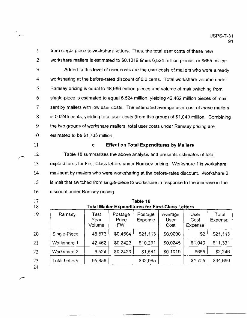
1
2
3
4
5
6
7
8
9
10
11
12 !-
13
14
15
16
17 18
19
20
21
22
23 24
USPS-T-31 91
from single-piece to workshare letters. Thus, the total user costs of these new
workshare mailers is estimated to $0.1019 times 6,524 million pieces, or $665 million.
Added to this level of user costs are the user costs of mailers who were already
worksharing at the before-rates discount of 6.0 cents. Total workshare volume under
Ramsey pricing is equal to 48,986 million pieces and volume of mail switching from
single-piece is estimated to equal 6,524 million, yielding 42,462 million pieces of mail
sent by mailers with low user costs. The estimated average u:ser cost of these mailers
is 0.0245 cents, yielding total user costs (from this group) of $‘I,040 million. Combining
the two groups of workshare mailers, total user costs under Ramsey pricing are
estimated to be $1,705 million.
C. Effect on Total Expenditures by Mailers
Table 18 summarizes the above analysis and presents ‘estimates of total
expenditures for First-Class letters under Ramsey pricing. Workshare 1 is workshare
mail sent by mailers who were worksharing at the before-rates discount. Workshare 2
is mail that switched from single-piece to workshare in response to the increase in the
discount under Ramsey pricing.
Table 18 Total Mailer Expenditures for First-Class Letters
Ramsey
Single-Piece
Workshare 1
Workshare 2
Total Letters
Test Postage Postage Year Price Expense
Volume FWI
46,873 $0.4504 $21 ,I 13
42,462 $0.2423 $10,291
6,524 $0.2423 $1,581
95.859 $32.985

USPS-T-31 ‘-’
1
2
3
4
5
6
I
8
9
10
11
12
13
14
15
16
17
18
19
20
21
22
23
24
25
92
Table 18 shows that under Ramsey pricing of single-piece and workshare letters,
mailers would pay $34,690 million to send 95,859 million pieces of mail. The average
expenditure per piece is $0.3619. At the before-rates prices, mailers sent 96,901
million pieces at an average expenditure per piece of $0.3521, equal to the before-rates
price including user costs. At the R9’7-1 non-Ramsey rates based on ‘the R94-1 mark-
ups, m,ailers sent 95,370 million pieces of First-Class letters at an average expenditure
per piece for First-Class letters is $0.3589, equal to the non-Ramsey postage price plus
the average user cost. Average expenditures under Ramsey pricing are higher,
because net revenues under Ramsey pricing are greater than under the before-rates
pricing schedule or the non-Ramsey rate schedule.
d. Net Gain from Efficient Pricing of Letter Categories
The total gain from Ramsey pricing of single-piece and workshare letters is given
by the (change in consumer and producer surplus, where the change in producer
surplus is the change in net revenues earned by the Postal Service. F:ealize that the
increase in net revenues earned by the Postal Service from First-Class letters is used to
satisfy ,the break-even constraint and provide lower prices for more elastic subclasses.
Table 19 presents the total change in social welfare, where the change in
consumer surplus is estimated using the simple approximation presented earlier in this
testimony. The change in producer surplus is the change in net reverrues. Changes in
consumer and producer surplus from the Ramsey pricing of single-piece and
workshared letters are measured relative to the before-rates price of letters and the
non-Ramsey price of letters.
Net revenues from First-Class letters are estimated to be $168’14 million (see
Table 17) before-rates. Net revenues from First-Class letters under the non-Ramsey
rate schedule are $16,603 (see Table 11). Net revenues from First-Class letters under -.

USPS-T-31 93
8
9 10 11
12 13
14 .r.
15
16
17
18
19
20
21
22
23
24
25
26
F!amsey pricing are $17,238 million. Total net gain is the sum of the change in
consumer surplus and net revenues.
Table 19 Total Gains from Ramsey Pricing of Single-Piece and Workshared Letters
Before-Rates Ramsey Change in Change in Net Total Net Gain Expenditures Expenditures Consumer Revenues per Piece per Piece Surplus
$0.3521 $0.3619 -$940 million
INon-Ramsey Ramsey Change in Expenditures Expenditures Consumer Revenues per Piece per Piece Surplus i
$1,424 million $484 million
Change in Net Total Net Gain
$0.3589 $0.36,19 -$287 million $635 million $348 million
Thus, efficient pricing of single-piece and workshared letters leads to a net gain
of between $348 million and $464 million, depending on whether the comparison is with
the before-rates price schedule or the non-Ramsey price schedule. With respect to the
non-Ramsey rate schedule, the $348 million net gain shown in Table 19 is in addition to
the $1,023 million gain in consumer surplus realized under Ramsey pricing of mail
subclasses.
E. Conclusions
Ramsey pricing is shown to be consistent with Efficient Colmponent Pricing when
the demands for single-piece and workshared letters are the same. When these
demands differ, the Ramsey efficient discount will differ from the ECP discount, with the
less elastic of the two First-Class letter categories assigned a higher per piece mark-up.
While this will lead to some inefficiency in mail sorting, the loss is less than the gain in
consumer surplus achieved through equalization of leakage acros.s the two products.

1
2
3
4
5
6
7
8
9
10
11
12
13
14
15
16
17
18
19
20
21
22
23
USPS-T-31 94
The extent to which the Ramsey discount departs from the ECP discount
depends largely on two considerations. First, the greater is the difference between the
own-plrice elasticities of the two categories of mail, the greater will be the difference in
the per piece mark-up of each category. Second, the smaller is the volume of mail that
shifts from single-piece to workshared (or vice versa), the less important is the discount
to overall efficiency. The empirical finding is that the difference between the ECP and
Ramsey discounts is small, owing to the fact that the own-price elastic:ities of single-
piece and workshared letters are not substantially different and to the fact that the
discoulnt does have a meaningful effect on the distribution of mail between single-piece
and workshared letters.
.Although the empirical results were illustrative, two points stancl out. It seems
reasonable to conclude that efficient pricing of the First-Class letter subclass would
involve an increase in the price of single-piece letters. A second finding is that the
discount for workshare mail should be increased to encourage greater mailer
worksharing, given the assumption that the resulting cost difference between single-
piece and workshared letters reflects the Postal Service’s savings.
Overall, it is found that efficient pricing of single-piece and workshared letters
produces a net gain of between $348 million and $484 million, above and beyond the
gains realized by Ramsey pricing of mail subclasses. The exact calcuKation of the net
gain depends on estimates of the user costs of mailers who switch frorn sending single-
piece to workshare letters. This is an important consideration, not just from Rarrsey or
Efficient Component Pricing, but for any pricing schedule that affects the assignment of
worksharing activities.
7